Embed Size (px)
DESCRIPTION
Top-down estimate of methane emissions in California using a mesoscale inverse modeling technique. - PowerPoint PPT Presentation
Citation preview

Top-down estimate of methane emissions in California using a mesoscale inverse
modeling technique
Yuyan Cui1,2
Jerome Brioude1,2, Stuart McKeen1,2, Wayne Angevine1,2, Si-Wan Kim1,2, Gregory J. Frost1,2, Ravan Ahmadov1,2, Jeff Peischl1,2, Thomas Ryerson1, Steve C. Wofsy3, Gregory W. Santoni3, Michael Trainer1,*
1. Chemical Sciences Division, Earth System Research Laboratory, NOAA, Boulder.2. Cooperative Institute for Research in Environmental Sciences, University of Colorado, Boulder.3. Department of Earth and Planetary Sciences, Harvard University, Cambridge.
The 13th CMAS Conference October 27-29, 2014UNC-Chapel Hill

Outline
Backgrounds, observations and the inversion method
Estimates of methane emissions from the posterior and prior inventories (NEI), over the South Coast Air Basin (SoCAB), CA
Preliminary results for methane emissions over Central Valley, CA

CH4 has increased by factor of 2.5 at least since pre-industrial times (IPCC AR5).
The atmospheric lifetime of CH4 of ~12 years, shorter than CO2 but with much higher global warming potential than CO2 (~72 times higher over 20 years, and ~25 times higher over 100 years).
The change in CH4 mixing ratio also likely altered the concentrations of OH and ozone in the troposphere and water vapor in the stratosphere.
In California, CH4 emissions are regulated by Assembly Bill 32, enacted into law as the California Global Warming Solutions Act of 2006, requiring the state’s greenhouse gas emissions in the year 2020 not to exceed 1990 emission levels.
Background

The South Coast Air Basin(SoCAB)
Central Valley
San Joaquin Valley
SacramentoValley
Six flights
Six flights
μg m-2 s-1NEI 2005NOAA P-3 research aircrafts
Wavelength- scanned cavity ring-down spectroscopy (Picarro 1301 m)
CalNex 2010 Airborne measurements
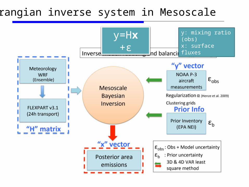
y=Hx +ε y: mixing ratio (obs)x: surface fluxes
Lagrangian inverse system in Mesoscale

Brioude et al. 2011
May 08 flight For each flight we give a background value
For each flight, we give a regularization α (Henze et al. 2009) to reach a good compromise in R and B
Costfunction
J obs J prior
R and B are covariance matrices
Bayesian formulation with lognormal distribution
s m3 kg−1 s m3 kg−1
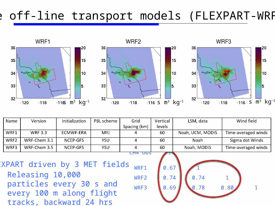
CH4 obs WRF1 WRF2 WRF3
CH4 Obs 1
WRF1 0.67 1
WRF2 0.74 0.74 1
WRF3 0.69 0.78 0.80 1
s m3 kg−1
Correlation R
FLEXPART driven by 3 MET fieldsReleasing 10,000 particles every 30 s and every 100 m along flight tracks, backward 24 hrs
Three off-line transport models (FLEXPART-WRF)

Log10The SoCAB
Log10 Central Valley
Bocquet el al. (2011)
J=Tr (BWTR-1W)
Based on Fisher information matrix, a criterion map is used to present the significance of each grid cell in constraining the CH4 emissions.
Clustering spatially grid cells

SoCAB ResultsCH4 flux in NEI 2005
Prior Inventory:CH4 emissions were processed following EPA recommendations in EPA SPECIATE 4.1 database (Simon et al. 2010).
μg m-2 s-1
CH
4 ab
ove
bkg
(ppb
)
# of Obs
ObservationFlexpart+prior
230 Gg /yr.
Underestimates0508 flight

Observation
Flexpart+prior
Flexpart+post
Optimization of CH4 mixing ratios
Mean bias: prior: 50ppbv post: 8ppbv R2: prior: 0.55 post: 0.7
0508 flight0508 flight
CH
4 ab
ove
bkg
(ppb
v)
Bias and correlation are improved using the posterior
Flight
Mean bias(ppbv)
R2 (WRF1) R2 (WRF2) R2 (WRF3)
Prior Post Prior post Prior post Prior post
0504 44.3 7.7 0.4 0.7 0.4 0.7 0.5 0.8
0508 49.9 7.9 0.5 0.6 0.6 0.7 0.5 0.6
0514 10.3 4.0 0.7 0.8 0.4 0.7 0.3 0.7
0516 35.9 7.8 0.5 0.6 0.5 0.5 0.3 0.4
0519 28.0 8.1 0.6 0.7 0.7 0.8 0.5 0.7
0620 24.5 3.2 0.6 0.7 0.4 0.7 0.4 0.7
Obs above bkg (ppbv)
mod
el a
bove
bkg
(ppb
v)
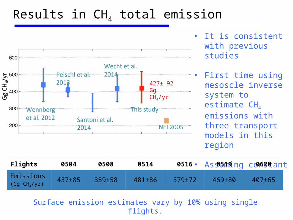
• It is consistent with previous studies
• First time using mesoscle inverse system to estimate CH4 emissions with three transport models in this region
• Assuming constant CH4 emissions in the urban region
Results in CH4 total emission
Flights 0504 0508 0514 0516 0519 0620
Emissions(Gg CH4/yr) 437±85 389±58 481±86 379±72 469±80 407±65
Surface emission estimates vary by 10% using single flights.
427± 92 Gg CH4/yr
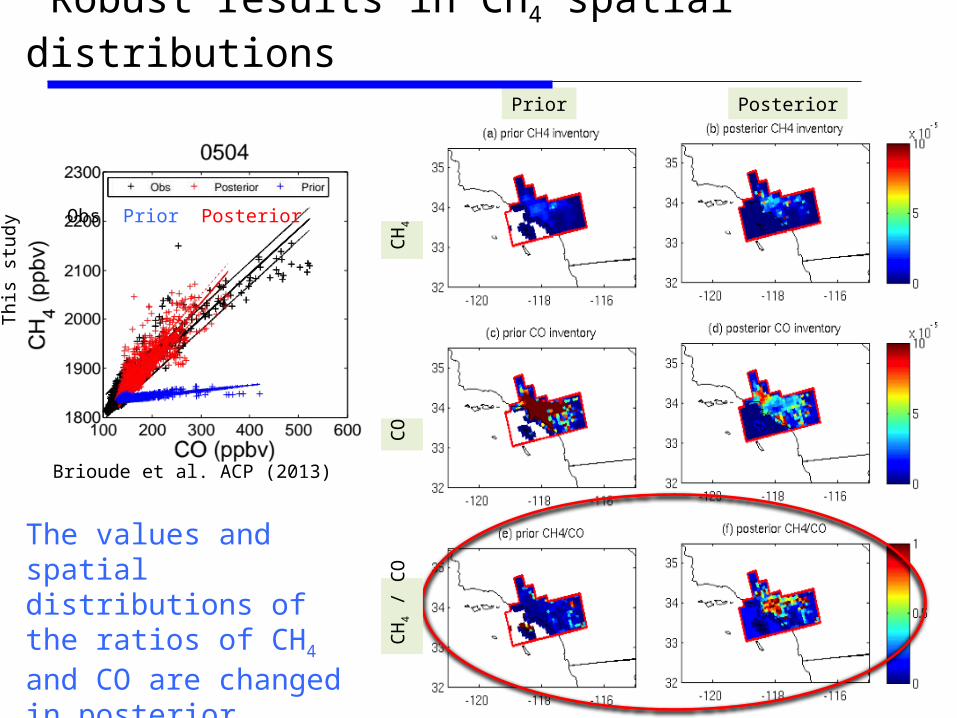
Robust results in CH4 spatial distributions
Brioude et al. ACP (2013)
This
stud
y
Prior Posterior
CH4
COCH
4 / C
O
Obs Prior Posterior
The values and spatial distributions of the ratios of CH4 and CO are changed in posterior inventory

CH4 source sectors
• CARB 08 & 09. • The contribution of the dairy sector is higher by factor of ~1.9 and ~1.6 than
bottom-up estimates (NEI05 and CARB09). Peischl et al. (2013)• The contribution of oil and gas wells, landfills, and point sources (297± 61
Gg/yr) is higher by factor of ~1.6 than the bottom-up estimates (NEI05).
52± 8 Gg /yr (upper bound)
Gg / yr Gg / yr
Gg / yr#
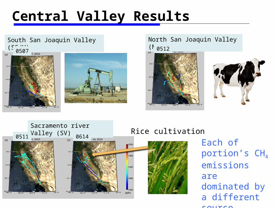
Central Valley Results
South San Joaquin Valley (SSJV) North San Joaquin Valley (NSJV)
Sacramento river Valley (SV)
0507
0511 0614
0512
Rice cultivationEach of portion’s CH4 emissions are dominated by a different source sectors.
40-
39-
38-
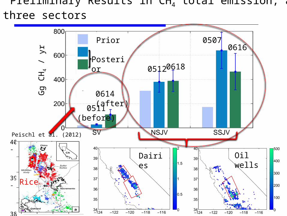
Preliminary Results in CH4 total emission, and three sectors
Oil wellsDairies
Rice
Prior
Posterior
0511 (before)
0614(after)
0512 0618
05070616
Gg
CH4 /
yr
Peischl et al. (2012)
Conclusions
• The mesoscale inverse method improve simulations of CH4 mixing ratios and the slopes of correlations between CH4 and CO.
• The total CH4 emissions in SoCAB estimated by the inverse system are consistent with previous top-down studies, and by factor of two higher than the prior inventory. This is the first estimate based on a mesoscale inversion method in this region.
• Our uncertainty estimates include the uncertainty of the inversion method and also the uncertainty from the transport models.
• The dairy and oil well sectors in the San Joaquin Valley seem to be underestimated by the prior inventory (NEI05).
Cui et al. 2014, in prep