Embed Size (px)
Citation preview

Volatility Jump Risk in the Cross-Section of Stock Returns
Yu Li
University of Houston
September 29, 2017
Abstract
Jumps in aggregate volatility has been established as an important factor affecting
the volatility dynamic, the market index price, and the index option price. However,
whether it affects the price of other assets is still an open question. This paper provides
supportive evidence in the individual equity market. We use a VIX option portfolio to
measure the volatility jump risk and test whether it is priced in the cross-section of
stock returns. We find a significant negative risk premium associated with the volatility
jump risk and it is robust after controlling for a bunch of systematic risk factors.

1 Introduction
While many studies have showed that jumps in aggregate volatility is an important
factor affecting the equilibrium asset price (Drechsler and Yaron (2011)), the volatility
dynamic (Corsi, Pirino, and Reno (2010), Jacod, Todorov et al. (2010), Todorov and
Tauchen (2011)), and the index option pricing (Eraker, Johannes, and Polson (2003),
Eraker (2004), Broadie, Chernov, and Johannes (2007)), its impact on the cross-section of
stock returns is less explored. This paper tries to fill the gap by constructing an empirical
measure about the volatility jump and test how the volatility jump affects the cross-section
of stock returns.
The cross-section of stock returns is important for at least two reasons. First, it reveals
the risk preference of market participants. Given the ample evidence of volatility jump on
the aggregate market level, it would be interesting to test its implication on the cross-section
of stock returns. Second, several recent studies have tested the role of price jumps on
the cross-section of stock returns. (see, for example, Babaoglu (2015), Bollerslev, Li, and
Todorov (2016), and Bollerslev, Li, and Zhao (2016)). Especially, Cremers, Halling, and
Weinbaum (2015) compare the impact of the aggregate price jump risk and the aggregate
volatility risk on the cross-section of stock returns. We would like to see whether the
aggregate volatility jump risk would affect their conclusion.
However, estimating the volatility jump risk is not easy. Previous papers usually employ
a fully specified model to filter out the volatility jumps. Thus the estimation results depend
on the model specification. In contrast, this paper uses a non-parametric method to estimate
the volatility jump risk. Our measure relies on few model assumptions and reflects the
market expectation about the future volatility jump risk.
Specifically, we use the return of a Delta-neutral, Vega-neutral, and Gamma-positive
VIX option portfolio to track the daily volatility jump risk. We treat VIX as a proxy for the
future expected market volatility. Although this proxy has a disadvantage because of the
embedded risk premium, it benefits us in the sense that we can observe market prices of
2

various traded derivatives on VIX. Moreover, VIX options are especially informative about
the higher moments so we use them to construct the volatility jump measure.
The volatility jump portfolio is a Delta-neutral, Vega-neutral, and Gamma-positive VIX
option strategy. We rely on the key insight proposed by Coval and Shumway (2001) and
Cremers, Halling, and Weinbaum (2015), which is different option Greeks reflect different
risks. In our case, Delta of VIX option measures the sensitivity of option price to the VIX
levels, thus it reflects the volatility risk. Vega measures the sensitivity of option price to
the volatility of VIX, thus it reflects the volatility of volatility risk. Gamma is the second
order derivative of VIX option price to the VIX level thus it captures the effect of large
VIX movements, i.e. the volatility jump risk. Because our portfolio is Delta-neutral and
Vega-neutral, so its return is immune to small changes of the volatility and the volatility of
volatility. The positive Gamma creates the exposure to large volatility movements. Thus the
price of this VIX option portfolio is mainly driven by the market expectation about future
large movements of the volatility. If the market expects more significant volatility jumps in
the future, the price would be high and otherwise it would be low.
We use this strategy to construct a daily volatility jump risk measure and test whether
it affects the cross-section of stock returns. We conduct both the sort exercise and the
Fama-MacBeth regression. Both methods show that the volatility jump risk is negatively
priced in the cross-section of stock returns. The return difference between the portfolio that
has lowest sensitivity to the volatility jump and the portfolio that has highest sensitivity is
about -7.9% per year. Fama-MacBeth regression estimates the risk premium is about -6.5%
per year. Furthermore, our results are robust after controlling for the volatility risk, the
volatility risk, the price jump risk, the idiosyncratic volatility, the idiosyncratic skewness,
the realized volatility, the co-skewness, the co-kurtosis, the upside beta, as well as the
downside beta. Our results are also robust for different sample periods as well as different
stock portfolios. Thus we provide supportive evidence that the volatility jump risk is indeed
priced in the cross-section of stock returns.
3

Our paper is related with several strands of literature. First, our paper is related with the
large literature which examines what are the systematic risk driving the cross-section of stock
returns. (see, for example, Fama and French (1993), Carhart (1997), Pástor and Stambaugh
(2003), Ang, Chen, and Xing (2006), Ang et al. (2006), Chang, Christoffersen, and Jacobs
(2013), and Cremers, Halling, and Weinbaum (2015)) We contribute by examining whether
the volatility jump risk is another systematic risk factor. Our paper also relates with the
recent literature which focuses on the higher moments of the volatility (Lin and Chang
(2009), Huang and Shaliastovich (2014), Agarwal, Arisoy, and Naik (2015), Song (2012),
Mencía and Sentana (2013), Lin (2013), Bakshi, Madan, and Panayotov (2015), Amengual
and Xiu (2016), Park (2016), Song and Xiu (2016)). We contribute by examining the
implication of volatility jump risk in the cross-section of stock return. Finally, our paper
is related with the paper which uses non-parametric method to estimate the jumps in the
volatility (Andersen, Bollerslev, and Diebold (2007), Jacod, Todorov et al. (2010), Corsi,
Pirino, and Reno (2010), Todorov and Tauchen (2011), Todorov, Tauchen, and Grynkiv
(2014), and Bandi and Reno (2016)). We contribute by proposing a volatility jump measure
using the VIX options.
This paper proceeds as follows. Section 2 describes the data and section 3 reports the
empirical methodology. Section 4 discusses the main results. Section 5 presents the robust
tests and section 6 concludes.
2 Data Description
Our main data, VIX futures options, is from OptionMetrics. For each day, we collect all
the VIX options maturing in the next calendar month and the month after that. We drop
the observation if it meets any one of the following criteria, (1) the bid price, ask price,
implied volatility, or any Greeks is missing, (2) the trade volume or open interest is zero,
(3) the bid price is greater than the offer price. In addition, we drop the data in the early
4

sample period because VIX options are not very liquid in the first several months.1 Our final
sample ranges from April 2nd, 2007 to August 31st, 2015, yielding to 2037 days in total.
As for other data, VIX futures are from the official website of CBOE. We collect the
daily close prices of VIX futures of all maturities and match them with the corresponding
options based on the option expiration date. We exclude the observation if the close price
of VIX futures is either zero or missing. Individual equity data is from CRSP. We clean it by
dropping all missing values and deleting all non-financial firms and non-common shares.
Daily and monthly Fama-French factors are from Prof. French’s website.
3 Empirical Methodology
In this section, we will first introduce the volatility jump risk measure and then the
empirical methodology.
3.1 Construct the Volatility Jump Risk Measure
Our volatility jump risk measure is the return of a Delta-neutral, Vega-neutral, and
Gamma-positive VIX option portfolio, which is constructed as follows. On each day, we
first rank all VIX calls and puts based on their moneyness, which is defined as the strike to
the underlying price ratio. Then we choose the closet ATM call and put pair to formulate a
ATM straddle. The weights of call and put are calculated as follow.
θCall,t + θPut,t = 1
θCall,t∆Call,t + θPut,t∆Put,t = 0(1)
where ∆Call,t is the market Delta of the call option at time t and ∆put,t is the market Delta
of the put option at time t. We conduct the above procedure for VIX options maturing in 1
1This is consistent with the existing literature such as Jackwerth and Vilkov (2015), Park (2015), andSong and Xiu (2016).
5

month and 2 months respectively, yielding to a 1 month straddle and a 2 month straddle
every day. The straddle returns are calculated as follows.
ret iSt raddle,t = θ
iCal l,t ret i
Cal l,t + θiPut,t ret i
Put,t i = 1,2 (2)
where ret iCal l,t is the return of the Call option maturing in month i and ret i
Put,t is the return
of the put option maturing in month i. Next we short 1 contract of 2 month straddle and
long δt contract of 1 month straddle. δt is solved by the following equation to make the
portfolio Vega-neutral.
δtν1t − ν
2t = 0 (3)
ν1t denotes the Vega of the 1 month straddle at time t and ν2
t denotes the Vega of the 2
month straddle at time t. Because short term options have larger Gamma than long term
options, the Gamma of this position is positive. On each day, we construct the position and
hold it for one day. On the next day, we sell the outstanding position formed on previous
day and reconstruct a new position using the same methodology. Thus, we can get a daily
measure of the volatility jump risk using the daily return of this portfolio, which can be
calculated as follows.
retVol Jump,t = δt ret1St raddle,t − ret2
St raddle,t (4)
retVol Jump,t would be high if market expects a high probability of the volatility jump and
would be low otherwise.
3.2 Test whether the Volatility Jump Risk is Priced
To prove the volatility jump risk is a priced systematic risk factor, we need to show a
contemporaneous relationship between the volatility jump beta and the portfolio returns.
We follow the empirical procedure in Ang et al. (2006) and Cremers, Halling, and Weinbaum
(2015) to detect the empirical relationship. The procedure is as follows.
6

For each individual stock i, on the end of each month, we regress its daily excess returns
on the daily excess returns of the market portfolio and the daily returns of the volatility
jump portfolio over the past 12 months.
Rit = α
i + β iMKTMKTt + β
iVol JumpVol Jumpt + ε
i (5)
where Rit is the excess return of stock i on time t, MKTt is the excess return of the market
portfolio on time t, and Vol Jumpt is the return of the volatility jump portfolio at time t.
We don’t control the SMB and HML factor in equation 5 to be consistent with Ang et al.
(2006), but our main results are robust for adding those two factors.
Then we sort the stocks into 5 portfolios based on the estimated β iVol Jump and calculate
the value-weighted and equal-weighted holding-period returns of each portfolio over the
same period, i.e. the past 12 months. Then we move to the next month and repeat the
exercise. As a result, we get a time-series of monthly returns for every portfolio. We
calculate Fama-French 3 factor α for each portfolio as follows.
R jt = α
j + β jMKTMKTt + β
jSMBSMBt + β
jHMLHMLt + εt , j = 1,2, ..., 5 (6)
where R jt is the holding-period return calculated in month t, MKTt is the holding-period
return of the market portfolio in month t, SMBt is the holding-period return of the SMB
portfolio in month t, and HMLt is the holding-period return of the HML portfolio in month
t.
We also run the Fama-Macbeth regression to estimate the risk premium. At each month,
we regress the excess return of each individual stock on the estimated β iMKT and β i
Vol Jump
over the past 12 months as follows.
Rit = γ0 + γVol Jump,t β̂
iVol Jump,t + γMKT,t β̂
iMKT,t + ε
i (7)
7

γVol Jump,t are averaged across time to get the final estimate. So does the t-stats. All the
standard errors are adjusted using Newey and West (1987) method with 12 lags.
4 Empirical Results
This section discusses our main results. We first check whether the volatility jump risk
measure that extracted from VIX options is consistent with the realized jump in VIX, then
we test whether the volatility jump risk is priced in the cross-section of stork returns by
using both the sorting exercise and cross-sectional regression exercise.
4.1 Volatility Jump Measures
To test whether the portfolio return tracks the large movement of volatility, we compare
it with the realized jumps of the volatility. We expect to see the portfolio return spikes
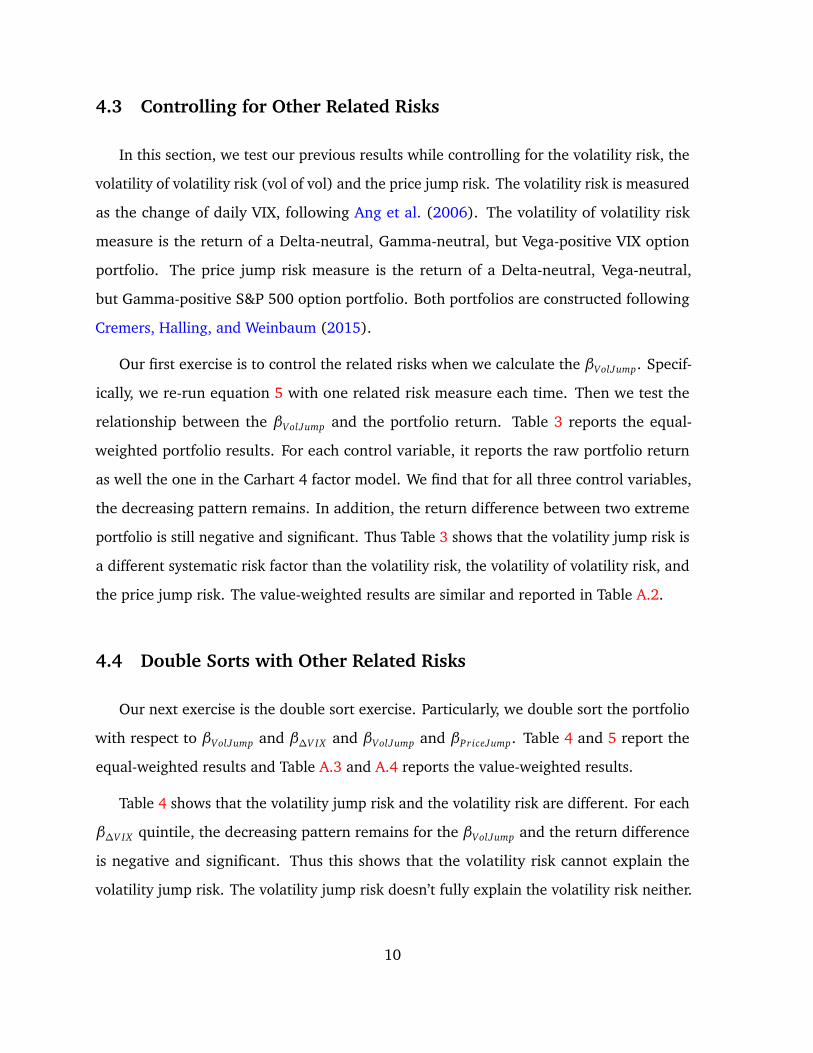
whenever a physical volatility jump occurs. Figure 1 plots the daily return of the volatility
jump portfolio (the solid line) and the days when jumps of VIX occurred (the vertical
dashed line). The realized jumps of VIX are identified by the Lee and Mykland (2008)
non-parametric method. The method procedure is given in the 6. In general, we find the
return peaks when VIX jumps occur, suggesting the volatility jump portfolio the volatility
jump risk.
Table 1 reports the statistical property of the volatility jump measure. Panel A reports
the summary statistics and Panel B reports the correlation coefficients of volatility jump
with other systematic factors.
The third column in Panel A shows the average return of the volatility jump portfolio is
negative, about -0.02% per year or -5.04% per year, suggesting a negative risk premium
for the volatility jump return. The negative return is consistent with the fact that the VIX
options are used as a hedge tool against the market downside drops, so investors are willing
to pay for holding the volatility jump portfolio. The fourth to sixth columns reports the
8

standard deviation, the daily minimum return and the maximum return. Large magnitudes
of those numbers suggest the volatility jump measure is time-varying and quite volatile.
The last two columns presents the skewness and kurtosis. Both number suggest that the
volatility jump measure is non-normal and follows a highly leptokurtic distribution.
Panel B shows the correlation coefficient between the volatility jump measure and other
related systematic risk factors. We find the coefficients are moderate except for the volatility
of volatility and the aggregate jump of S&P 500. This suggests that the volatility jump is
closely correlated with the volatility of volatility and the price jump.
4.2 Portfolio Sorting Results
Table 2 reports average returns of the equal-weighted portfolios sorted by the βVolJump.
It reports the raw return as well as the return in the CAPM model, in the Fama-French
3-factor model, as well as in the Cahart 4-factor model. Given the negative risk premium
of volatility jump which is shown in Table 1, we should observe a decreasing relationship
between the βVolJump and the portfolio returns, i.e. the higher the βVolJump, the lower the
portfolio return. More importantly, the difference between the return of the portfolio that
has the highest βVolJump with the portfolio that has the lowest βVolJump should be negative
and significant. And this difference should not be explained by other existing risk factors.
This is exactly what we find in Table 2. First we find that on average, there is a decreasing
pattern between the portfolio return and the Table 2. The portfolio with a higher sensitivity
to the volatility jump risk earns a lower return, consistent with the hedging story. Moreover,
we find the difference between the portfolio 5 and 1 is about -7.9% per year and significant
on the 1% percent level. Furthermore, the negative alpha persists across in the CAPM
model, the FF3 model, as well as the Carhart 4 model. Overall, we find our results provide
strong evidence showing that the volatility jump risk is negatively priced in the cross-section
of stock returns. The return of value-weighted portfolio are in the Table A.1.
9
4.3 Controlling for Other Related Risks
In this section, we test our previous results while controlling for the volatility risk, the
volatility of volatility risk (vol of vol) and the price jump risk. The volatility risk is measured
as the change of daily VIX, following Ang et al. (2006). The volatility of volatility risk
measure is the return of a Delta-neutral, Gamma-neutral, but Vega-positive VIX option
portfolio. The price jump risk measure is the return of a Delta-neutral, Vega-neutral,
but Gamma-positive S&P 500 option portfolio. Both portfolios are constructed following
Cremers, Halling, and Weinbaum (2015).
Our first exercise is to control the related risks when we calculate the βVolJump. Specif-
ically, we re-run equation 5 with one related risk measure each time. Then we test the
relationship between the βVolJump and the portfolio return. Table 3 reports the equal-
weighted portfolio results. For each control variable, it reports the raw portfolio return
as well the one in the Carhart 4 factor model. We find that for all three control variables,
the decreasing pattern remains. In addition, the return difference between two extreme
portfolio is still negative and significant. Thus Table 3 shows that the volatility jump risk is
a different systematic risk factor than the volatility risk, the volatility of volatility risk, and
the price jump risk. The value-weighted results are similar and reported in Table A.2.
4.4 Double Sorts with Other Related Risks
Our next exercise is the double sort exercise. Particularly, we double sort the portfolio
with respect to βVolJump and β∆V IX and βVolJump and βPriceJump. Table 4 and 5 report the
equal-weighted results and Table A.3 and A.4 reports the value-weighted results.
Table 4 shows that the volatility jump risk and the volatility risk are different. For each
β∆V IX quintile, the decreasing pattern remains for the βVolJump and the return difference
is negative and significant. Thus this shows that the volatility risk cannot explain the
volatility jump risk. The volatility jump risk doesn’t fully explain the volatility risk neither.
10

We find the volatility risk is also priced for each volatility jump risk quintile. This shows
that the volatility risk contains another component, which is consistent with the fact that
the volatility of volatility risk is also priced.
Table 5 shows that the volatility jump risk and the price jump risk are somewhat
correlated. For example, the Carhart 4 alpha of βVolJump portfolio are only significant in the
first two quintiles of βPriceJump. This could be due to the fact that there is a strong co-jump
structure of the S&P 500 and the VIX.
4.5 Fama-Macbeth Regression
In this section, we estimate the risk premium associated with the volatility jump using
the Fama-Macbeth regression. Table 6 reports the results in the CAPM model as well as
the Carhart 4 factor model. We find that the coefficient of volatility jump is significantly
negative. The magnitude is about -0.5% per month, or -6% per year. The coefficient cannot
be explained by other market variables. Table 7 shows that the coefficient controlling for a
bunch of stock characteristics. We find the stock characteristics affect the magnitude of
estimated coefficients, they cannot explain the significance level. So the volatility jump risk
is both different from the market factors and the firm characteristics.
5 Robust Test
This section investigates whether different regression specification alter our conclusion.
We re-examine our results using different estimation periods, in different samples, and
with different portfolios.
11

5.1 Different Estimation Periods
First we alter the estimation periods for getting the βVolJump. We change the estimation
period to 3 months, 6 months, as well as 24 months. Table 8 shows both the equal-weighted
and value-weighted results. We find the results hold for all three specifications.
5.2 Different Sample Periods
We also find that our results hold for different sample periods. Table 8 reports the
equal-weighted and value-weighted portfolio returns in 2007 to 2011 and 2012 to 2015.
The same pattern shows in both periods. Particularly, the return difference is larger and
more significant in the first sample period. This is consistent with the fact that the effect of
volatility jump risk is stronger when the market is more volatile.
5.3 Different Portfolios
Finally, we test whether the volatility jump risk can explain the other portfolio returns.
We repeat our exercise with the Fama-French 25 portfolios sorted on size and book-to-
market as well as the 49 industry portfolio. Table 10 shows the average return as well as
the Carhart 4 alpha. We find for both portfolios, the alphas are significant and robust for
the other market risk factors.
6 Concluding Remarks
In summary, this paper studies the impact of market volatility jump risk on the cross-
section of stock returns. We measure the volatility jump risk using the VIX options and find
it’s priced in the individual equity market. We show that the volatility jump risk carries a
negative risk premium. The risk premium is robust for different empirical specifications,
different sample periods, and different stock portfolios. Our results imply that the volatility
12

jump risk is another important risk factor and it’s independent of the volatility risk, the
volatility of volatility risk, and the price jump risk.
13

References
Agarwal, V., Y. E. Arisoy, and N. Y. Naik. 2015. Volatility of aggregate volatility and hedge
funds returns. Working Paper, CFR Working Paper.
Amengual, D., and D. Xiu. 2016. Resolution of policy uncertainty and sudden declines in
volatility .
Andersen, T. G., T. Bollerslev, and F. X. Diebold. 2007. Roughing it up: Including jump
components in the measurement, modeling, and forecasting of return volatility. The
review of economics and statistics 89:701–20.
Ang, A., J. Chen, and Y. Xing. 2006. Downside risk. Review of Financial Studies 19:1191–239.
Ang, A., R. J. Hodrick, Y. Xing, and X. Zhang. 2006. The cross-section of volatility and
expected returns. The Journal of Finance 61:259–99.
Babaoglu, K. G. 2015. The pricing of market jumps in the cross-section of stocks and options
.
Bakshi, G., D. Madan, and G. Panayotov. 2015. Heterogeneity in beliefs and volatility tail
behavior. Journal of Financial and Quantitative Analysis 50:1389–414.
Bandi, F. M., and R. Reno. 2016. Price and volatility co-jumps. Journal of Financial Economics
119:107–46.
Bollerslev, T., S. Z. Li, and V. Todorov. 2016. Roughing up beta: Continuous versus dis-
continuous betas and the cross section of expected stock returns. Journal of Financial
Economics 120:464–90.
Bollerslev, T., S. Z. Li, and B. Zhao. 2016. Good volatility, bad volatility and the cross-section
of stock returns .
Broadie, M., M. Chernov, and M. Johannes. 2007. Model specification and risk premia:
Evidence from futures options. The Journal of Finance 62:1453–90.
14

Carhart, M. M. 1997. On persistence in mutual fund performance. The Journal of finance
52:57–82.
Chang, B. Y., P. Christoffersen, and K. Jacobs. 2013. Market skewness risk and the cross
section of stock returns. Journal of Financial Economics 107:46–68.
Corsi, F., D. Pirino, and R. Reno. 2010. Threshold bipower variation and the impact of
jumps on volatility forecasting. Journal of Econometrics 159:276–88.
Coval, J. D., and T. Shumway. 2001. Expected option returns. The journal of Finance
56:983–1009.
Cremers, M., M. Halling, and D. Weinbaum. 2015. Aggregate jump and volatility risk in
the cross-section of stock returns. The Journal of Finance 70:577–614.
Drechsler, I., and A. Yaron. 2011. What’s vol got to do with it. Review of Financial Studies
24:1–45.
Eraker, B. 2004. Do stock prices and volatility jump? reconciling evidence from spot and
option prices. The Journal of Finance 59:1367–403.
Eraker, B., M. Johannes, and N. Polson. 2003. The impact of jumps in volatility and returns.
The Journal of Finance 58:1269–300.
Fama, E. F., and K. R. French. 1993. Common risk factors in the returns on stocks and
bonds. Journal of financial economics 33:3–56.
Huang, D., and I. Shaliastovich. 2014. Volatility-of-volatility risk .
Jackwerth, J. C., and G. Vilkov. 2015. Asymmetric volatility risk: Evidence from option
markets. Available at SSRN 2325380 .
Jacod, J., V. Todorov, et al. 2010. Do price and volatility jump together? The Annals of
Applied Probability 20:1425–69.
15

Lee, S. S., and P. A. Mykland. 2008. Jumps in financial markets: A new nonparametric test
and jump dynamics. Review of Financial studies 21:2535–63.
Lin, Y.-N. 2013. Vix option pricing and cboe vix term structure: A new methodology for
volatility derivatives valuation. Journal of Banking & Finance 37:4432–46.
Lin, Y.-N., and C.-H. Chang. 2009. Vix option pricing. Journal of Futures Markets 29:523–43.
Mencía, J., and E. Sentana. 2013. Valuation of vix derivatives. Journal of Financial Economics
108:367–91.
Newey, W. K., and K. D. West. 1987. A simple, positive semi-definite, heteroskedasticity
and autocorrelation consistent covariance matrix. Econometrica 55:703–08.
Park, Y.-H. 2015. Volatility-of-volatility and tail risk hedging returns. Journal of Financial
Markets 26:38–63.
———. 2016. The effects of asymmetric volatility and jumps on the pricing of vix derivatives.
Journal of Econometrics 192:313–28.
Pástor, L., and R. F. Stambaugh. 2003. Liquidity risk and expected stock returns. Journal of
Political economy 111:642–85.
Song, Z. 2012. Expected vix option returns .
Song, Z., and D. Xiu. 2016. A tale of two option markets: Pricing kernels and volatility risk.
Journal of Econometrics 190:176–96.
Todorov, V., and G. Tauchen. 2011. Volatility jumps. Journal of Business & Economic Statistics
29:356–71.
Todorov, V., G. Tauchen, and I. Grynkiv. 2014. Volatility activity: Specification and estimation.
Journal of Econometrics 178:180–93.
16

Figu
re1
Dai
lyR
etu
rns
ofth
eVo
lati
lity
Jum
pPo
rtfo
lio
This
figur
epl
ots
the
daily
retu
rns
ofth
evo
lati
lity
jum
ppo
rtfo
lio.
The
vola
tilit
yju
mp
port
folio
isa
Del
ta-n
eutr
al,V
ega-
neut
ral,
and
Gam
ma
posi
tive
VIX
opti
onpo
rtfo
lio,w
hich
isco
nsis
ted
wit
ha
ATM
VIX
stra
ddle
mat
urin
gin
1m
onth
and
aAT
MV
IXst
radd
lem
atur
ing
in2
mon
ths.
The
retu
rnof
the
vola
tilit
yju
mp
port
folio
posi
tive
lyre
late
sw
ith
the
jum
pm
agni
tude
ofV
IX.
Vert
ical
dash
edlin
esre
pres
ents
the
larg
est
100
jum
psin
VIX
,whi
char
ees
tim
ated
usin
gth
e5
min
utes
high
freq
uenc
yda
taof
VIX
byLe
ean
dM
ykla
nd(2
008)
met
hod.
2008
2009
2010
2011
2012
2013
Tim
e
-0.3
-0.2
-0.10
0.1
0.2
Res
idu
als
of
Ret
urn
s o
f th
e V
ola
tilit
y Ju
mp
Po
rtfo
lioR
ealiz
ed J
um
ps
of
VIX
by
Lee
an
d M
ykla
nd
(20
08)
Tes
t
17

Table 1Summary Statistics of Daily Returns of the Volatility Jump Portfolio
This table reports the summary statistics of daily returns of the volatility jump portfolio(Vol Jump). Panel A reports the number of observations, the daily average return, thedaily median return, the standard deviation, the minimum, the maximum, the skewness,the kurtosis, and the autocorrelation coefficient. Panel B reports the Pearson correlationcoefficients of Vol Jump with the level of VIX, the change of VIX (∆V IX ), the return of aVIX portfolio tracking the change of volatility of volatility (Vol of Vol), the return of a SPXportfolio tracking the change of jumps in S&P 500 (Price Jump), the market excess return(MKT), the SMB factor (SMB), the HML factor (HML), and the momentum factor (UMD).The sample period is from April, 2007 to August 2015.
Panel A: Summary Statistics
N Mean Median Std Deviation Min Max Skewness Kurtosis AR(1)
Vol Jump 2077 -0.02% -0.56% 4.04% -19.77% 45.07% 2.18 14.32 -0.04
Panel B: Pairwise Correlation Coefficients
Vol Jump VIX ∆VIX Vol of Vol Price Jump MKT SMB HML UMD
Vol Jump 1.00
VIX 0.04 1.00
∆VIX 0.29 0.10 1.00
Vol of Vol −0.68 −0.01 −0.13 1.00
Price Jump 0.48 0.09 0.40 −0.28 1.00
MKT −0.19 −0.13 −0.84 0.10 −0.25 1.00
SMB 0.01 −0.02 −0.07 0.04 −0.01 0.17 1.00
HML −0.04 −0.08 −0.29 0.03 −0.09 0.43 −0.02 1.00
UMD −0.05 −0.01 0.23 0.04 −0.01 −0.41 −0.01 −0.59 1.00
18

Table 2Equal-weighted Returns of Sorted Portfolios
This table reports the average return, CAPM alpha, Fama-French 3 factor alpha, andCarhart4 factor alpha of the equal-weighted portfolio sorted on βVolJump. On each month,we regress the excess returns of each individual stock over the next 12 months on thereturns of the volatility jump portfolio, controlling for the market excess returns. Thenwe sort the stocks in to 5 portfolio based on the βVolJump loading and calculate theequal-weighted average return in the 12 months. Portfolio 1 has the lowest βVolJump
loadings and Portfolio 5 has the highest βVolJump loadings. Returns are annualized andstandard errors are adjusted by Newey and West (1987) method with 12 lags. T-statisticsare reported in the parenthesis. The sample period is from April, 2007 to August 2015.
EW Portfolio Average Return CAPM Alpha FF 3 Alpha Carhart4 Alpha
1 Low βVol Jump 21.85 11.65 6.04 9.11
(3.38) (1.73) (3.12) (7.65)
2 16.89 8.96 5.44 6.95
(3.27) (2.39) (4.70) (13.87)
3 15.66 8.18 4.58 6.21
(3.13) (2.09) (3.59) (11.17)
4 16.49 8.49 3.91 6.05
(3.09) (1.63) (2.93) (7.76)
5 High βVol Jump 13.95 4.21 -1.70 1.28
(2.05) (0.56) (-0.79) (1.53)
5-1 -7.90*** -7.44*** -7.74*** -7.83***
(-4.94) (-5.98) (-11.25) (-13.81)
19

Table 3Equal-weighted Returns of Sorted Portfolios Controlling for Other Risk Factors
This table reports the average return and Carhart4 factor alpha of the equal-weightedportfolio sorted on βVolJump, while controlling for other risk factors. The empiricalprocedure is the same as in Table 2, but we control other risk factors in the time seriesestimation. Specifically, we control the change of VIX (∆V IX ), the return of a VIX optionportfolio tracking the volatility of volatility risk (Vol of Vol), and the return of a SPXoption portfolio tracking the aggregate price jump risk (Price Jump). Portfolio 1 has thelowest βVolJump loadings and Portfolio 5 has the highest βVolJump loadings. Returns areannualized and standard errors are adjusted by Newey and West (1987) method with 12lags. T-statistics are reported in the parenthesis. The sample period is from April, 2007 toAugust 2015.
X = ∆V IX X = Vol of Vol X = Price Jump
EW Portfolio Average Return Carhart4 Alpha Average Return Carhart4 Alpha Average Return Carhart4 Alpha
1 Low βVol Jump 20.13 7.75 19.23 6.52 19.93 6.64
(3.19) (5.86) (2.86) (9.44) (2.99) (8.42)
2 17.49 7.52 17.52 8.14 16.50 6.47
(3.42) (13.46) (3.53) (16.13) (3.15) (13.43)
3 15.74 6.19 16.75 7.43 16.83 7.25
(3.13) (11.19) (3.46) (13.48) (3.51) (13.39)
4 16.17 5.74 16.08 5.52 15.77 5.26
(3.00) (11.61) (3.03) (6.48) (2.95) (7.42)
5 High βVol Jump 15.06 2.33 14.81 1.60 15.69 3.67
(2.16) (2.84) (2.23) (1.44) (2.37) (2.58)
5 -1 -5.07*** -5.42*** -4.42*** -4.92*** -4.24** -2.96***
(-2.90) (-5.83) (-3.75) (-5.02) (-2.52) (-2.85)
20

Table 4Equal-weighted Returns of Double Sorted Portfolios on βVolJump and β∆V IX
This table reports the Carhart4 factor alpha of the equal-weighted portfolio double sortedon βVolJump and β∆V IX . On each month, we regress the excess returns of each individualstock over the next 12 months on the returns of the volatility jump portfolio and thechange of VIX, controlling for the market excess returns. Then we double sort the stocks into 5 portfolio based on the βVolJump loading and on the β∆V IX loading. We calculate theequal-weighted average return in the 12 months for each of the 25 portfolios and theCarhart4 factor alpha. Portfolio 1 has the lowest βVolJump loadings and Portfolio 5 has thehighest βVolJump loadings. Returns are annualized and standard errors are adjusted byNewey and West (1987) method with 12 lags. T-statistics are reported in the parenthesis.The sample period is from April, 2007 to August 2015.
Carhart4 Alpha 1 Low β∆VIX 2 3 4 5 High β∆VIX 5-1
1 Low βVol Jump 10.62 10.57 8.72 7.05 2.58 -8.04***
(8.12) (10.25) (9.46) (5.84) (1.10) (-3.56)
2 10.10 9.97 7.37 6.87 4.90 -5.20***
(8.40) (12.50) (8.61) (8.51) (3.74) (-5.42)
3 9.01 9.10 7.56 5.74 1.87 -7.14***
(8.67) (10.72) (8.79) (10.54) (3.30) (-7.85)
4 8.49 7.39 6.78 5.37 0.30 -8.19***
(10.61) (8.13) (9.39) (9.63) (0.38) (-7.35)
5 High βVol Jump 2.93 5.94 2.75 0.62 -1.64 -4.57**
(1.64) (4.45) (2.97) (0.70) (-1.21) (-2.34)
5 - 1 -7.70*** -4.63*** -5.97*** -6.43*** -4.22**
(-6.15) (-2.91) (-4.96) (-5.04) (-2.59)
21

Table 5Equal-weighted Returns of Double Sorted Portfolios on βVolJump and βPriceJump
This table reports the Carhart4 factor alpha of the equal-weighted portfolio double sortedon βVolJump and βPriceJump. On each month, we regress excess returns of each individualstock over the next 12 months on returns of the volatility jump portfolio and returns ofthe price jump portfolio, controlling for the market excess returns. Then we double sortthe stocks in to 5 portfolio based on the βVolJump loading and on the βPriceJump loading.We calculate the equal-weighted average return in the 12 months for each of the 25portfolios and the Carhart4 factor alpha. Portfolio 1 has the lowest βVolJump loadings andPortfolio 5 has the highest βVolJump loadings. Returns are annualized and standard errorsare adjusted by Newey and West (1987) method with 12 lags. T-statistics are reported inthe parenthesis. The sample period is from April, 2007 to August 2015.
Carhart4 Alpha 1 Low βPrice Jump 2 3 4 5 High βPrice Jump 5-1
1 Low βVol Jump 12.23 11.05 6.20 4.04 0.59 -11.64***
(7.65) (10.73) (9.74) (4.00) (0.28) (-4.55)
2 10.27 8.73 7.64 6.95 2.06 -8.22***
(8.19) (12.39) (19.09) (11.17) (2.63) (-6.43)
3 10.26 9.23 7.85 7.18 2.41 -7.85***
(6.34) (10.65) (11.86) (21.16) (4.20) (-4.67)
4 7.26 8.01 7.30 4.71 1.15 -6.11***
(4.02) (8.08) (10.02) (8.14) (1.37) (-3.12)
5 High βVol Jump 2.31 5.03 4.88 2.65 -2.93 -5.24
(1.18) (2.86) (3.24) (2.60) (-1.11) (-1.57)
5 - 1 -9.92*** -6.02*** -1.32 -1.38 -3.52
(-4.43) (-4.02) (-1.00) (-0.94) (-1.51)
22

Table 6Fama-MacBeth Regression Controlling for ∆VIX, Vol of Vol, and the Price Jump
This table reports the Fama-Macbeth regression results. On each month, we regress excessreturns of each individual stock over the next 12 months on returns of the volatilityjump portfolio, while controlling for different factors. Then we conduct Fama-Macbethregression on each month. Standard errors are adjusted by Newey and West (1987)method with 12 lags. T-statistics are reported in the parenthesis. The sample period isfrom April, 2007 to August 2015.
CAPM Model Carhart4 Factor Model
Vol Jump −0.55∗∗∗ −0.48∗∗∗ −0.33∗∗ −0.47∗∗∗ −0.50∗∗∗ −0.49∗∗∗ −0.34∗∗ −0.39∗∗
(−5.57) (−4.25) (−2.15) (−2.88) (−4.83) (−4.19) (−2.30) (−2.58)
MKT 0.01 0.01 0.01 0.02 0.01 0.01 0.01 0.02
(1.11) (1.12) (0.97) (1.37) (1.41) (1.30) (1.41) (1.58)
∆VIX −2.14∗∗ −2.40∗∗
(−1.76) (−2.28)
Vol of Vol 0.00 0.00
(1.15) (1.15)
Price Jump −0.15∗∗∗ −0.11∗∗∗
(−3.39) (−2.88)
SMB 0.00 0.01 0.00 0.00
(0.98) (1.08) (1.07) (0.98)
HML 0.00 (0.00) (0.01) (0.00)
(−0.03) (−0.20) (−0.72) (−0.54)
UMD 0.03∗ 0.03∗ 0.03∗ 0.03∗
(1.93) (1.95) (1.82) (1.94)
Constant 0.05∗ 0.05∗ 0.05∗∗ 0.05∗ 0.05∗ 0.05∗ 0.05∗ 0.05∗
(1.92) (1.92) (2.01) (1.75) (1.85) (1.93) (1.91) (1.74)
23

Table 7Fama MacBeth Regression with Other Control Variables
This table reports the Fama-Macbeth regression results with other control variables. Wecontrol the idiosyncratic volatility, idiosyncratic skewness, realized volatility, coskewness,cokurtosis, upside beta, and downside beta. Standard errors are adjusted by Newey andWest (1987) method with 12 lags. T-statistics are reported in the parenthesis. The sampleperiod is from April, 2007 to August 2015.
CAPM Model Carhart4 Factor Model
βVol Jump βVol Jump
Idio. Vol -0.18∗∗∗ -0.11∗∗
(-3.75) (-2.16)
Idio. Skew -0.16∗∗∗ -0.10∗∗
(-4.57) ( -2.17)
Realized Vol -0.18∗∗∗ -0.11∗∗
(-3.76) (-2.17)
CoSkew -0.23∗∗∗ -0.17∗∗∗
(-4.53) (-3.16)
CoKurt -0.20∗∗∗ -0.14∗∗
-4.24 -2.43
Upside Beta -0.21∗∗∗ -0.14∗∗
(-4.59) (-2.75)
Downside Beta -0.26∗∗∗ -0.21∗∗∗
(-7.82) (-4.31)
24

Table 8Robust Results with Different Estimation Length
This table reports the Carhart4 factor alpha of both equal-weighted and value-weightedportfolio with different estimation length. Portfolio 1 has the lowest βVolJump loadings andPortfolio 5 has the highest βVolJump loadings. Returns are annualized and standard errorsare adjusted by Newey and West (1987) method with 12 lags. T-statistics are reported inthe parenthesis. The sample period is from April, 2007 to August 2015.
3 Months 6 Months 24 Months
EW Carhart4 Alpha VW Carhart4 Alpha EW Carhart4 Alpha VW Carhart4 Alpha EW Carhart4 Alpha VW Carhart4 Alpha
1 Low βVol Jump 5.60 0.21 6.15 2.26 6.55 13.06
(1.64) (0.06) (2.42) (0.99) (4.79) (13.16)
2 3.79 3.49 7.13 5.97 10.30 8.23
(1.97) (2.06) (5.51) (6.66) (20.38) (33.23)
3 4.67 5.67 5.45 4.89 8.10 8.07
(3.36) (3.70) (4.42) (3.68) (20.36) (52.38)
4 1.57 2.40 2.75 2.18 5.69 2.97
(1.01) (1.22) (1.79) (1.65) (14.62) (10.02)
5 High βVol Jump 0.07 -1.15 1.25 -3.02 -1.08 -3.28
(0.02) (-0.38) (0.64) (-1.68) (-1.12) (-3.87)
5 - 1 -5.54** -1.35 -4.90*** -5.27* -7.63*** -16.34***
(-2.59) (-0.26) (-3.349) (-1.85) (-11.89) (-42.11)
25

Table 9Robust Results with Sub-samples
This table reports the estimated Carhart4 factor alpha in subsamples. The first sampleis from April 2007 to December 2011. The second is from January 2012 to December2015. For each period, we report the Carhart4 factor alpha of both the equal-weightedportfolio and the value-weighted portfolio. Portfolio 1 has the lowest βVolJump loadings andPortfolio 5 has the highest βVolJump loadings. Returns are annualized and standard errorsare adjusted by Newey and West (1987) method with 12 lags. T-statistics are reported inthe parenthesis. The sample period is from April, 2007 to August 2015.
2007 - 2011 2012 - 2015
EW Portfolio Average Return CAPM Alpha FF3 Alpha Average Return CAPM Alpha FF3 Alpha
1 8.61 8.38 4.44 9.35 3.96 2.31
Low βVol Jump (1.01) (1.91) (1.56) (1.90) (1.32) (1.36)
2 6.55 6.27 3.46 8.05 3.63 2.66
(1.02) (2.31) (2.06) (2.20) (2.01) (2.83)
3 5.88 5.59 2.74 7.48 3.34 2.37
(0.97) (2.08) (1.91) (2.24) (1.97) (3.19)
4 5.14 4.87 1.37 6.77 2.32 1.26
(0.77) (1.57) (0.88) (1.86) (1.22) (1.64)
5 4.85 4.63 0.35 7.02 1.50 0.16
High βVol Jump (0.56) (1.03) (0.13) (1.40) (0.51) (0.10)
5 - 1 −3.76∗∗∗ −3.76∗∗∗ −4.10∗∗∗ −2.33∗∗∗ −2.45∗∗∗ −2.14∗∗
(−9.40) (−9.66) (−8.65) (−2.85) (−2.82) (−2.56)
26

Table 10Robust Results with Fama-French 25 Portfolios and Industry 49 Portfolios
This table reports the average return and the Carhart 4 alpha of Fama-French 25 Size andBook-to-Market portfolios and the 49 industry portfolios. Portfolio 1 has the lowest βVolJump
loadings and Portfolio 5 has the highest βVolJump loadings. Returns are annualized andstandard errors are adjusted by Newey and West (1987) method with 12 lags. T-statisticsare reported in the parenthesis. The sample period is from April, 2007 to August 2015.
25 FF Portfolios 49 Industry Portfolios
EW Portfolio Average Return CAPM Alpha FF3 Alpha Average Return CAPM Alpha FF3 Alpha
1 6.30 1.96 1.90 6.63 2.62 2.26
Low βVol Jump (1.85) (1.98) (3.08) (2.07) (2.76) (2.28)
2 5.54 1.43 1.16 6.42 2.61 2.11
(1.69) (1.14) (1.87) (2.09) (2.87) (3.54)
3 5.41 1.34 0.97 5.34 1.34 0.97
(1.71) (1.19) (2.22) (1.66) (1.26) (1.43)
4 4.78 0.85 0.48 4.99 0.84 0.58
(1.53) (0.67) (0.99) (1.51) (0.86) (0.94)
5 3.74 −0.40 −0.80 3.29 −1.05 −1.35
High βVol Jump (1.13) (−0.36) (−1.85) (0.94) (−0.86) (−1.88)
5 - 1 −2.56∗∗∗ −2.37∗∗∗ −2.71∗∗∗ −3.35∗∗∗ −3.67∗∗∗ −3.61∗∗∗
(−3.29) (−3.16) (−3.73) (−3.23) (−3.23) (−3.46)
27

Appendix
A.1 Lee and Mykland (2008) Non-Parametric Method
Following Lee and Mykland (2008), we calculate the statistics L(i) as follows.
L(i) =logV IX (t i)/V IX (t i−1)
σ̂(t i)(8)
where
σ̂(t i) =1
K − 2
i−1∑
j=i−K+2
|logV IX (t j)/V IX (t j−1)|logV IX (t j−1)/V IX (t j−2)| (9)
V IX (t i) is the closing price of VIX at time t i and K is the length of the rolling window.
Because we use daily observations, we let K = 16 as suggested by the original paper. The
threshold for |L(i)−Cn|Sn
is β , where
Cn =(2logn)0.5
c−
logπ+ log(logn)2c(2logn)0.5
(10)
and
Sn =1
c(2logn)0.5(11)
.
n is the number of observations, β = −log(−log(1− Significance Level)).
28

Table A.1Value-weighted Returns of Sorted Portfolios
This table reports the average return, CAPM alpha, Fama-French 3 factor alpha, andCarhart4 factor alpha of the value-weighted portfolio sorted on βVolJump. On each month,we regress the excess returns of each individual stock over the next 12 months on thereturns of the volatility jump portfolio, controlling for the market excess returns. Thenwe sort the stocks in to 5 portfolio based on the βVolJump loading and calculate thevalue-weighted average return in the 12 months. Portfolio 1 has the lowest βVolJump
loadings and Portfolio 5 has the highest βVolJump loadings. Returns are annualized andstandard errors are adjusted by Newey and West (1987) method with 12 lags. T-statisticsare reported in the parenthesis. The sample period is from April, 2007 to August 2015.
VW Portfolio Average Return CAPM Alpha FF 3 Alpha Carhart4 Alpha
1 Low βVol Jump 16.00 8.28 6.08 6.66
(2.82) (5.01) (5.56) (6.26)
2 12.92 6.76 6.21 6.48
(2.55) (12.41) (10.87) (11.00)
3 13.16 7.52 6.32 7.10
(3.17) (6.01) (9.70) (12.22)
4 11.75 4.54 1.96 3.45
(2.56) (1.37) (1.71) (2.78)
5 High βVol Jump 9.82 0.26 -5.55 -3.62
(1.51) (0.04) (-2.84) (-1.80)
5 - 1 -6.18 -8.02* -11.63*** -10.27***
(-1.58) (-1.80) (-5.49) (-4.83)
29

Table A.2Value-weighted Returns of Sorted Portfolios Controlling for Other Risk Factors
This table reports the average return and Carhart4 factor alpha of the value-weightedportfolio sorted on βVolJump, while controlling for other risk factors. The empiricalprocedure and the control variables are the same as in Table 3. Portfolio 1 has thelowest βVolJump loadings and Portfolio 5 has the highest βVolJump loadings. Returns areannualized and standard errors are adjusted by Newey and West (1987) method with 12lags. T-statistics are reported in the parenthesis. The sample period is from April, 2007 toAugust 2015.
X = ∆V IX X = Vol of Vol X = Price Jump
VW Portfolio Average Return Carhart4 Alpha Average Return Carhart4 Alpha Average Return Carhart4 Alpha
1 Low βVol Jump 16.15 7.86 16.49 7.81 14.29 4.83
(3.29) (6.03) (3.18) (8.93) (2.61) (8.20)
2 12.62 5.64 12.53 6.52 12.73 5.97
(2.41) (7.78) (2.48) (9.64) (2.43) (8.31)
3 13.07 6.84 12.23 5.50 13.23 7.18
(2.87) (8.53) (3.06) (8.56) (3.15) (10.86)
4 12.43 4.97 12.87 4.41 13.29 5.39
(2.79) (6.98) (2.83) (3.60) (3.06) (4.83)
5 High βVol Jump 10.94 (1.65) 10.05 (3.50) 11.14 -1.24
(1.69) (-1.10) (1.54) (-1.42) (1.90) (-0.56)
5 - 1 -5.21 -9.51*** -6.45* -11.31*** -3.15 -6.07***
(-1.32) (-8.19) (-1.82) (-5.82) (-0.93) (-3.19)
30

Table A.3Value-weighted Returns of Double Sorted Portfolios on βVolJump and β∆V IX
This table reports the Carhart4 factor alpha of the value-weighted portfolio double sortedon βVolJump and β∆V IX . On each month, we regress the excess returns of each individualstock over the next 12 months on the returns of the volatility jump portfolio and thechange of VIX, controlling for the market excess returns. Then we double sort the stocks into 5 portfolio based on the βVolJump loading and on the β∆V IX loading. We calculate thevalue-weighted average return in the 12 months for each of the 25 portfolios and theCarhart4 factor alpha. Portfolio 1 has the lowest βVolJump loadings and Portfolio 5 has thehighest βVolJump loadings. Returns are annualized and standard errors are adjusted byNewey and West (1987) method with 12 lags. T-statistics are reported in the parenthesis.The sample period is from April, 2007 to August 2015.
Carhart4 Alpha 1 Low β∆VIX 2 3 4 5 High β∆VIX 5-1
1 Low βVol Jump 9.02 11.58 6.07 1.58 -0.71 -9.73**
(3.38) (9.60) (4.23) (0.96) (-0.17) (-2.39)
2 11.28 8.40 6.05 3.61 -3.89 -15.17***
(8.71) (10.04) (5.79) (3.00) (-3.33) (-7.98)
3 10.76 9.59 6.68 5.33 -0.66 -11.42***
(7.18) (9.11) (7.80) (6.35) (-0.71) (-4.92)
4 9.26 7.20 4.89 -0.73 -4.54 -13.80***
(7.26) (6.41) (6.28) (-0.45) (-3.76) (-7.08)
5 High βVol Jump 6.17 2.29 -2.01 -0.15 -8.53 -14.70***
(2.45) (1.26) (-0.77) (-0.10) (-8.39) (-5.26)
5 - 1 -2.85 -9.29*** -8.07*** -1.74 -7.82*
(-0.72) (-5.96) (-2.93) (-0.98) (-1.78)
31

Table A.4Value-weighted Returns of Double Sorted Portfolios on βVolJump and βPriceJump
This table reports the Carhart4 factor alpha of the value-weighted portfolio double sortedon βVolJump and βPriceJump. On each month, we regress excess returns of each individualstock over the next 12 months on returns of the volatility jump portfolio and returns of theprice jump portfolio, controlling for the market excess returns. Then we double sort thestocks in to 5 portfolio based on the βVolJump loading and on the βPriceJump loading. Wecalculate the value-weighted average return in the 12 months for each of the 25 portfoliosand the Carhart4 factor alpha. Portfolio 1 has the lowest βVolJump loadings and Portfolio 5has the highest βVolJump loadings. Returns are annualized and standard errors are adjustedby Newey and West (1987) method with 12 lags. T-statistics are reported in the parenthesis.The sample period is from April, 2007 to August 2015.
Carhart4 Alpha 1 Low βPrice Jump 2 3 4 5 High βPrice Jump 5-1
1 Low βVol Jump 18.78 9.27 1.62 -0.47 -1.08 -19.85***
(4.04) (5.92) (1.16) (-0.38) (-0.46) (-4.61)
2 11.71 6.20 6.09 6.93 2.50 -9.21***
(7.57) (6.21) (7.82) (9.43) (3.05) (-5.53)
3 11.79 8.01 7.67 6.19 -0.36 -12.15***
(8.58) (7.96) (11.13) (8.68) (-0.35) (-6.98)
4 8.48 6.51 5.84 2.76 -1.34 -9.82***
(3.91) (5.58) (7.81) (1.99) (-0.53) (-2.86)
5 High βVol Jump 0.75 3.00 0.76 -3.66 -6.39 -7.13**
(0.33) (0.97) (0.52) (-1.58) (-2.56) (-2.51)
-18.03*** -6.27* -0.86 -3.19 -5.31***
(-3.44) (-1.98) (-0.42) (-1.57) (-2.78)
32