Embed Size (px)
Citation preview

High performance numerical linear algebra:trends and new challenges.
Yousef SaadDepartment of Computer Science
and Engineering
University of Minnesota
HPC days in LyonApril 8, 2016
First: A personal tribute
ä Grenoble [not far off from here] was the place to be inscientific computing in the 1960’s and 1970’s
ä Jean Kuntzmann [1912-1992] and Noel Gastinel [1925-1984]played a huge role in Grenoble’s pre-eminence in NumericalAnalysis and Computer Science in France and Europe
HPC Days 04/08/2016 p. 2
Introduction: Numerical Linear Algebra
Numerical linear algebra has always been a “universal” tool inscience and engineering. Its focus has changed over the yearsto tackle “new challenges”
1940s–1950s: Major issue: the flutter problem in aerospaceengineering. Focus: eigenvalue problem.
ä Triggered discoveries of the LR and QR algorithms, and thepackage Eispack followed a little later
1960s: Problems related to the power grid promoted what weknow today as general sparse matrix techniques.
1970s: Finite Element methods, Computational Fluid Dynam-ics, reinforced need for general sparse techniques
HPC Days 04/08/2016 p. 3

Late 1980s – 1990s: Focus on parallel matrix computations.
Late 1990s: Big spur of interest in “financial computing” (Afterwhich the stock market collapsed ...)
ä Computational Mechanics (e.g., Fluid Dynamics, structures)has been a driving force in past few decades
ä But new forces are reshaping numerical linear algebra
Recent/Current: Google page rank, data mining, problemsrelated to internet technology, knowledge discovery, bio-informatics,nano-technology, ...
HPC Days 04/08/2016 p. 4
ä Major factor: Synergy between disciplines.
Example: Discoveries in materials (e.g. semi conductors re-placing vacuum tubes in 1950s) lead to faster computers, whichin turn lead to better physical simulations..
ä What about data-mining and materials?
ä Potential for a perfect union
ä A lot of recent interest
HPC Days 04/08/2016 p. 5
The plan:
1 The traditional: Sparse iterative solvers
– a brief tutorial
– recent research
2 The challenging: Materials science
– a brief tutorial
– solving very large eigenvalue problems
3 The new: Data Mining/ Machine learning
– a brief overview
– dimension reduction
HPC Days 04/08/2016 p. 6

PART 1: SPARSE ITERATIVE SOLVERS

Introduction: Linear System Solvers
General
Purpose
Specialized
Direct sparse Solvers
Iterative
A x = b∆ u = f− + bc
Methods Preconditioned Krylov
Fast PoissonSolvers
MultigridMethods
HPC Days 04/08/2016 p. 8

Long standing debate: direct vs. iterative
ä Starting in the 1970’s: huge progress of sparse direct solvers
ä Iterative methods - much older - not designed for ‘generalsystems’. Big push in the 1980s with help from ‘preconditioning’
ä General consensus now: Direct methods do well for 2-Dproblems and some specific applications [e.g., structures, ...]
ä Usually too expensive for 3-D problems
ä Huge difference between 2-D and 3-D case
ä Test: Two Laplacean matrices of same dimension n =122, 500. First: on a 350 × 350 grid (2D); Second: on a50× 50× 49 grid (3D)
HPC Days 04/08/2016 p. 9

ä Pattern of a similar [much smaller] coefficient matrix
0 100 200 300 400 500 600 700 800 900
0
100
200
300
400
500
600
700
800
900
nz = 4380
Finite Diff. Laplacean 30x30
0 100 200 300 400 500 600 700 800 900
0
100
200
300
400
500
600
700
800
900
nz = 5740
Finite Diff. Laplacean 10x10x9
HPC Days 04/08/2016 p. 10
A few observations
ä Problems are getting harder for Sparse Direct methods(more 3-D models, much bigger problems,..)
ä Problems are also getting difficult for iterative methodsCause: more complex models - away from Poisson
ä Researchers on both camps are learning each other’s tricksto develop preconditioners.
Current Challenges:
(1) Scalable (HPC) performance [for general systems]
(2) Robustness, general purpose preconditioners
HPC Days 04/08/2016 p. 11

Background: Preconditioned Krylov subspace methods
Two ingredients:
• An accelerator: Conjugate gradient, BiCG, GMRES,BICGSTAB,.. [‘Krylov subspace methods’]• A preconditioner: makes the system easier tosolve by accelator, e.g. Incomplete LU factorizations;SOR/SSOR; Multigrid, ...
One viewpoint:
ä Goal of preconditioner: generate good basic iterates.. [Gauss-Seidel, ILU, ...]
ä Goal of accelerator: find best combination of these iterates
HPC Days 04/08/2016 p. 12
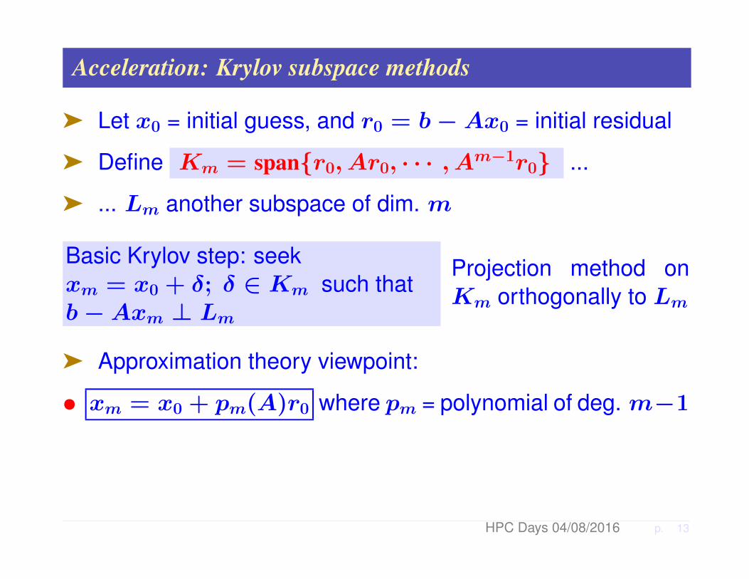
Acceleration: Krylov subspace methods
ä Let x0 = initial guess, and r0 = b−Ax0 = initial residual
ä Define Km = spanr0, Ar0, · · · , Am−1r0 ...
ä ... Lm another subspace of dim. m
Basic Krylov step: seekxm = x0 + δ; δ ∈ Km such thatb−Axm ⊥ Lm
Projection method onKm orthogonally to Lm
ä Approximation theory viewpoint:
• xm = x0 + pm(A)r0 where pm = polynomial of deg. m−1
HPC Days 04/08/2016 p. 13
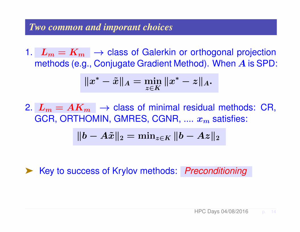
Two common and imporant choices
1. Lm = Km → class of Galerkin or orthogonal projectionmethods (e.g., Conjugate Gradient Method). WhenA is SPD:
‖x∗ − x‖A = minz∈K‖x∗ − z‖A.
2. Lm = AKm → class of minimal residual methods: CR,GCR, ORTHOMIN, GMRES, CGNR, .... xm satisfies:
‖b−Ax‖2 = minz∈K ‖b−Az‖2
ä Key to success of Krylov methods: Preconditioning
HPC Days 04/08/2016 p. 14
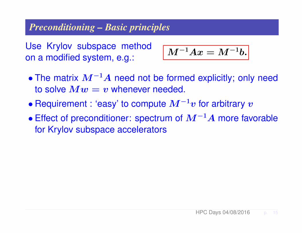
Preconditioning – Basic principles
Use Krylov subspace methodon a modified system, e.g.: M−1Ax = M−1b.
• The matrix M−1A need not be formed explicitly; only needto solve Mw = v whenever needed.
• Requirement : ‘easy’ to compute M−1v for arbitrary v
• Effect of preconditioner: spectrum of M−1A more favorablefor Krylov subspace accelerators
HPC Days 04/08/2016 p. 15

Both A and M are SPD: Preconditioned CG (PCG)
ALGORITHM : 1 Preconditioned Conjugate Gradient
1. Compute r0 := b−Ax0, z0 = M−1r0, and p0 := z0
2. For j = 0, 1, . . ., until convergence Do:3. αj := (rj, zj)/(Apj, pj)4. xj+1 := xj + αjpj5. rj+1 := rj − αjApj6. zj+1 := M−1rj+1
7. βj := (rj+1, zj+1)/(rj, zj)8. pj+1 := zj+1 + βjpj9. EndDo
ä Krylov method for M−1Ax = M−1b but use M -innerproduct to preserve self-adjointness.
HPC Days 04/08/2016 p. 16
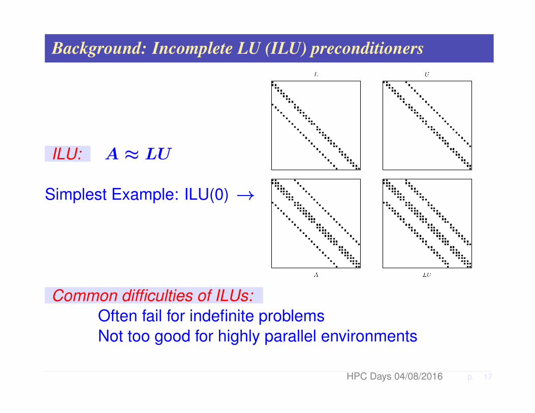
Background: Incomplete LU (ILU) preconditioners
ILU: A ≈ LU
Simplest Example: ILU(0) →
Common difficulties of ILUs:Often fail for indefinite problemsNot too good for highly parallel environments
HPC Days 04/08/2016 p. 17
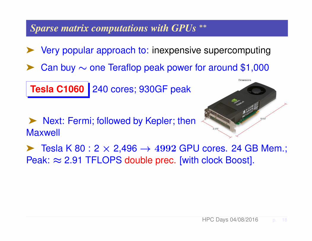
Sparse matrix computations with GPUs ∗∗
ä Very popular approach to: inexpensive supercomputing
ä Can buy∼ one Teraflop peak power for around $1,000
Tesla C1060 240 cores; 930GF peak
ä Next: Fermi; followed by Kepler; thenMaxwell
ä Tesla K 80 : 2 × 2,496→ 4992 GPU cores. 24 GB Mem.;Peak: ≈ 2.91 TFLOPS double prec. [with clock Boost].
HPC Days 04/08/2016 p. 18

The CUDA environment: The big picture
ä A host (CPU) and an attached device (GPU)
Typical program:
1. Generate data on CPU2. Allocate memory on GPU
cudaMalloc(...)3. Send data Host→ GPU
cudaMemcpy(...)4. Execute GPU ‘kernel’:kernel <<<(...)>>>(..)5. Copy data GPU→CPU
cudaMemcpy(...) C P U
G P
U
HPC Days 04/08/2016 p. 19
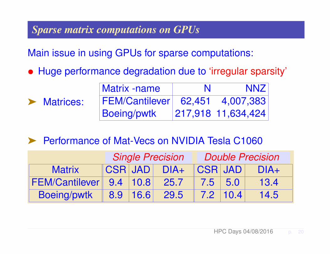
Sparse matrix computations on GPUs
Main issue in using GPUs for sparse computations:
• Huge performance degradation due to ‘irregular sparsity’
ä Matrices:Matrix -name N NNZFEM/Cantilever 62,451 4,007,383Boeing/pwtk 217,918 11,634,424
ä Performance of Mat-Vecs on NVIDIA Tesla C1060
Single Precision Double PrecisionMatrix CSR JAD DIA+ CSR JAD DIA+
FEM/Cantilever 9.4 10.8 25.7 7.5 5.0 13.4Boeing/pwtk 8.9 16.6 29.5 7.2 10.4 14.5
HPC Days 04/08/2016 p. 20
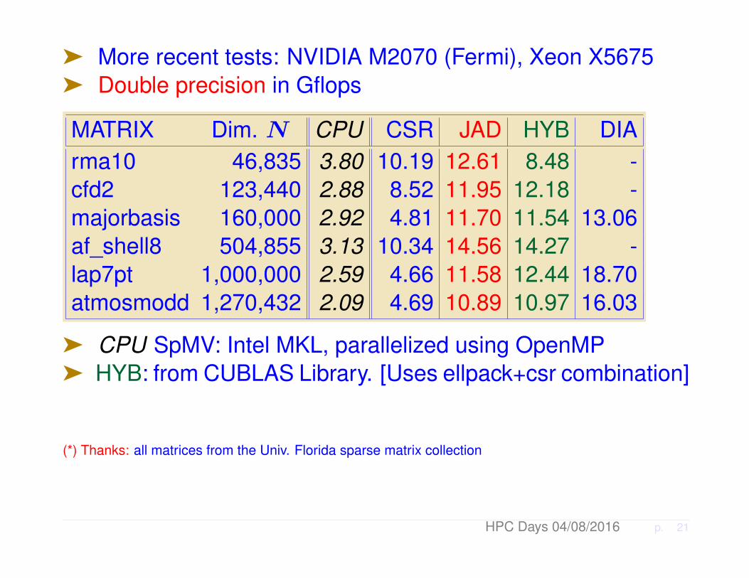
ä More recent tests: NVIDIA M2070 (Fermi), Xeon X5675ä Double precision in Gflops
MATRIX Dim. N CPU CSR JAD HYB DIArma10 46,835 3.80 10.19 12.61 8.48 -cfd2 123,440 2.88 8.52 11.95 12.18 -majorbasis 160,000 2.92 4.81 11.70 11.54 13.06af_shell8 504,855 3.13 10.34 14.56 14.27 -lap7pt 1,000,000 2.59 4.66 11.58 12.44 18.70atmosmodd 1,270,432 2.09 4.69 10.89 10.97 16.03
ä CPU SpMV: Intel MKL, parallelized using OpenMPä HYB: from CUBLAS Library. [Uses ellpack+csr combination]
(*) Thanks: all matrices from the Univ. Florida sparse matrix collection
HPC Days 04/08/2016 p. 21

Sparse Forward/Backward Sweeps
ä Next major ingredient of precond. Krylov subs. methods
ä ILU preconditioningoperations require L/Usolves: x← U−1L−1xä Sequential outer loop.
for i=1:nfor j=ia(i):ia(i+1)
x(i) = x(i) - a(j)*x(ja(j))end
end
ä Parallelism can be achieved with level scheduling:
• Group unknowns into levels
• Compute unknowns x(i) of same level simultaneously
• 1 ≤ nlev ≤ n
HPC Days 04/08/2016 p. 22
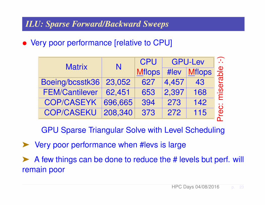
ILU: Sparse Forward/Backward Sweeps
• Very poor performance [relative to CPU]
Matrix NCPU GPU-Lev
Mflops #lev MflopsBoeing/bcsstk36 23,052 627 4,457 43FEM/Cantilever 62,451 653 2,397 168COP/CASEYK 696,665 394 273 142COP/CASEKU 208,340 373 272 115
Pre
c:m
iser
able
:-)
GPU Sparse Triangular Solve with Level Scheduling
ä Very poor performance when #levs is large
ä A few things can be done to reduce the # levels but perf. willremain poor
HPC Days 04/08/2016 p. 23
So...
... prepare for the demise of the GPUs...
... or the demise of the ILUs ?
HPC Days 04/08/2016 p. 24

Alternative: Low-rank approximation preconditioners
• Goal: use standardDomain Decompositionframework• Exploit Low-rank correc-tions• Consider a domain par-titioned in p sub-domainsusing vertex- based parti-tioniong (edge-separator)ä Interface nodes in eachdomain are listed last. 32 4 5
7 8 9 10
11 12 13 15
17 18
21 22 23 24 25
201916
6
1
14
HPC Days 04/08/2016 p. 25

The global system: Global view
ä Global system can bepermuted to the form→ä ui’s internal variablesä y interface variables
External interface points
Interior points
pointsLocal interface
B1 . . . F1
B2 . . . F2... . . . ...
Bp FpET
1 ET2 . . . ET
p C
u1
u2...upy
= b
ä Fi maps local interface points tointerior points in domain Ωi
ä ETi does the reverse operation
HPC Days 04/08/2016 p. 26
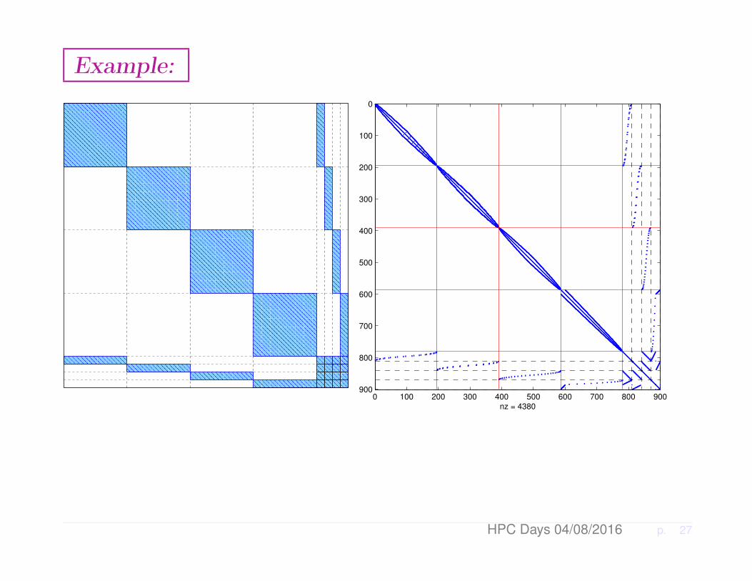
Example:
0 100 200 300 400 500 600 700 800 900
0
100
200
300
400
500
600
700
800
900
nz = 4380
HPC Days 04/08/2016 p. 27
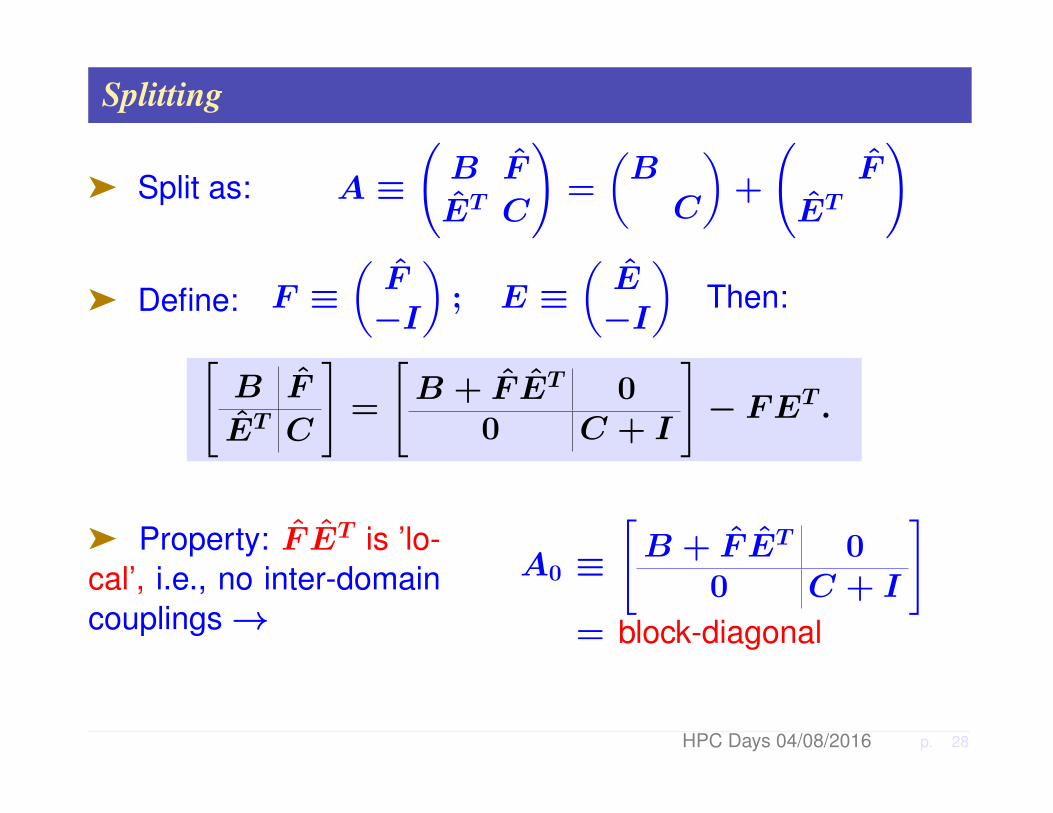
Splitting
ä Split as: A ≡(B F
ET C
)=
(BC
)+
(F
ET
)
ä Define: F ≡(F−I
); E ≡
(E−I
)Then:[
B F
ET C
]=
[B + F ET 0
0 C + I
]− FET .
ä Property: F ET is ’lo-cal’, i.e., no inter-domaincouplings→
A0 ≡[B + F ET 0
0 C + I
]= block-diagonal
HPC Days 04/08/2016 p. 28

Low-Rank Approximation DD preconditioners
Sherman-Morrison→ A−1 = A−10 +A−1
0 FG−1ETA−10
G ≡ I − ETA−10 F
Options: (a) Approximate A−10 F,ETA−1
0 , G−1
(b) Approximate only G−1 [this talk]
ä (b) requires 2 solves with A0.
Let G ≈ Gk
Preconditioner→M−1 = A−1
0 +A−10 FG−1
k ETA−1
0
HPC Days 04/08/2016 p. 29

Symmetric Positive Definite case
ä Recap: Let G ≡ I − ETA−10 E ≡ I −H . Then
A−1 = A−10 +A−1
0 EG−1ETA−10
ä Approximate G−1 by G−1k → preconditioner:
M−1 = A−10 + (A−1
0 E)G−1k (ETA−1
0 )
ä Matrix A0 is SPD
ä Can show: 0 ≤ λj(H) < 1 .
HPC Days 04/08/2016 p. 30

ä Now take rank-k approximation to H :H ≈ UkDkU
Tk Gk = I − UkDkU
Tk →
G−1k ≡ (I − UkDkU
Tk )−1 = I + Uk[(I −Dk)
−1 − I]UTk
ä Observation: A−1 = M−1 +A−10 E[G−1 −G−1
k ]ETA−10
ä Gk: k largest eigenvalues of H matched – others set == 0
ä Result: AM−1 has• n− s+ k eigenvalues == 1• All others between 0 and 1
HPC Days 04/08/2016 p. 31

Alternative: reset lowest eigenvalues to constant
ä Let H = UΛUT = exact (full) diagonalization of H
ä We replaced Λ by:
λ1
λ2. . .
λk0
. . .0
ä Alternative: replace Λ by
λ1
λ2. . .
λkθ
. . .θ
ä Interesting case: θ = λk+1
ä Question: related approximation to G−1?
HPC Days 04/08/2016 p. 32

ä Result: Let γ = 1/(1− θ). Then approx. to G−1 is:
G−1k,θ ≡ γI + Uk[(I −Dk)
−1 − γI]UTk
ä Gk: k largest eigenvalues of G matched – others set == θ
ä θ = 0 yields previous case
ä When λk+1 ≤ θ < 1 we get
ä Result: AM−1 has• n− s+ k eigenvalues == 1• All others≥ 1
ä Next: An example for a 900 × 900 Laplacean, 4 domains,s = 119.
HPC Days 04/08/2016 p. 33

Eigenvalues of AM−1. Used: k = 5 . Two cases
θ = 0
0.1 0.2 0.3 0.4 0.5 0.6 0.7 0.8 0.9 1 1.1−2.5
−2
−1.5
−1
−0.5
0
0.5
1
1.5
2
2.5x 10
−12
θ = λk+1
0.5 1 1.5 2 2.5 3 3.5 4 4.5−4
−3
−2
−1
0
1
2
3
4x 10
−12
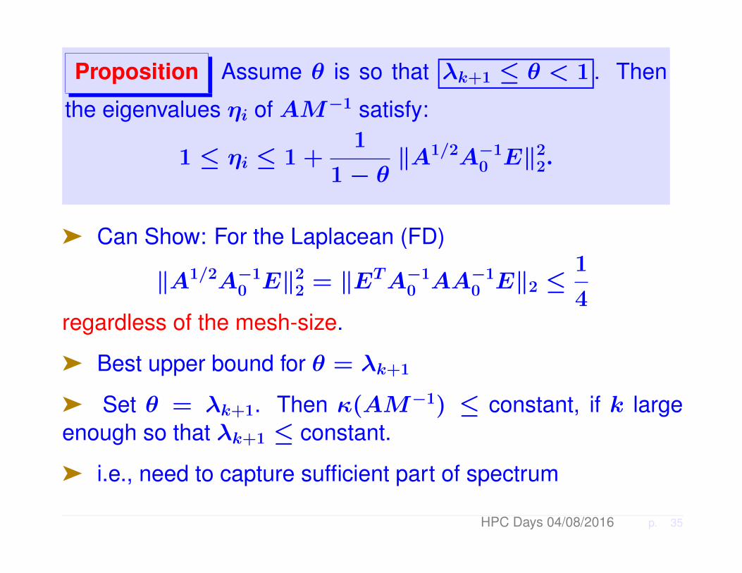
Proposition Assume θ is so that λk+1 ≤ θ < 1 . Then
the eigenvalues ηi of AM−1 satisfy:
1 ≤ ηi ≤ 1 +1
1− θ‖A1/2A−1
0 E‖22.
ä Can Show: For the Laplacean (FD)
‖A1/2A−10 E‖2
2 = ‖ETA−10 AA−1
0 E‖2 ≤1
4regardless of the mesh-size.
ä Best upper bound for θ = λk+1
ä Set θ = λk+1. Then κ(AM−1) ≤ constant, if k largeenough so that λk+1 ≤ constant.
ä i.e., need to capture sufficient part of spectrum
HPC Days 04/08/2016 p. 35
The symmetric indefinite case
ä Appeal of this approach over ILU: approximate inverse→Not as sensitive to indefiniteness
ä Part of the results shown still hold
ä But λi(H) can be > 1 now.
ä Can change the setting slightly [by introducing a parameterα] to improve diagonal dominance
ä Details skipped.
HPC Days 04/08/2016 p. 36
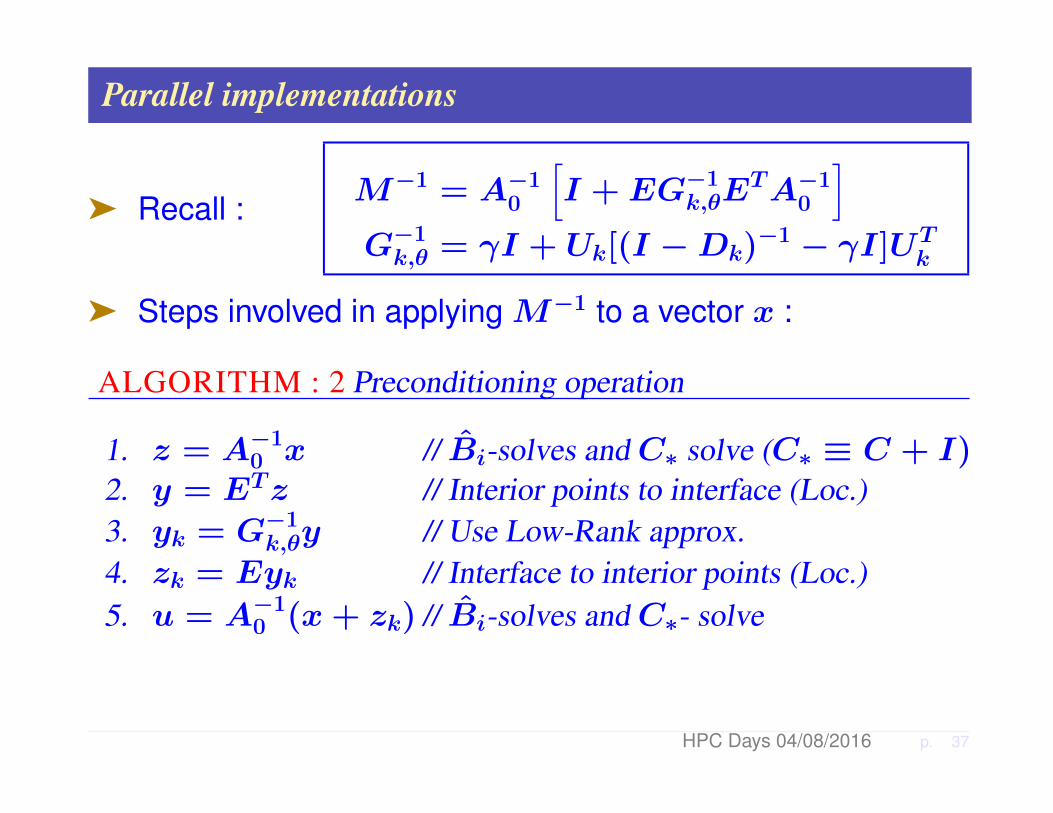
Parallel implementations
ä Recall : M−1 = A−10
[I + EG−1
k,θETA−1
0
]G−1k,θ = γI + Uk[(I −Dk)
−1 − γI]UTk
ä Steps involved in applying M−1 to a vector x :
ALGORITHM : 2 Preconditioning operation
1. z = A−10 x // Bi-solves andC∗ solve (C∗ ≡ C + I)
2. y = ETz // Interior points to interface (Loc.)3. yk = G−1
k,θy // Use Low-Rank approx.4. zk = Eyk // Interface to interior points (Loc.)5. u = A−1
0 (x+ zk) // Bi-solves andC∗- solve
HPC Days 04/08/2016 p. 37
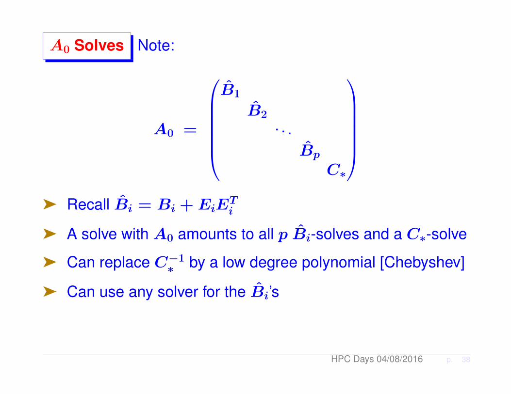
A0 Solves Note:
A0 =
B1
B2. . .
Bp
C∗
ä Recall Bi = Bi + EiE
Ti
ä A solve with A0 amounts to all p Bi-solves and a C∗-solve
ä Can replace C−1∗ by a low degree polynomial [Chebyshev]
ä Can use any solver for the Bi’s
HPC Days 04/08/2016 p. 38
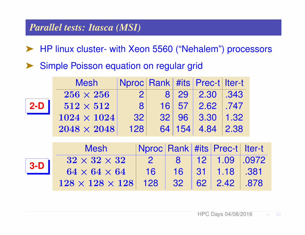
Parallel tests: Itasca (MSI)
ä HP linux cluster- with Xeon 5560 (“Nehalem”) processors
ä Simple Poisson equation on regular grid
2-D
Mesh Nproc Rank #its Prec-t Iter-t256× 256 2 8 29 2.30 .343512× 512 8 16 57 2.62 .747
1024× 1024 32 32 96 3.30 1.322048× 2048 128 64 154 4.84 2.38
3-D
Mesh Nproc Rank #its Prec-t Iter-t32× 32× 32 2 8 12 1.09 .097264× 64× 64 16 16 31 1.18 .381
128× 128× 128 128 32 62 2.42 .878
HPC Days 04/08/2016 p. 39

PART 2: ALGORITHMS FOR ELECTRONIC STRUCTURE

Approximations/theories used
ä Original Schrödinger equation very complex
ä Approximations developed started the 1930s reached ex-cellent level of accuracy. Among them...
Density Functional Theory: (DFT) observable quantities areuniquely determined by ground state charge density.
Kohn-Sham equation:
[−∇2
2+ Vion + VH + Vxc
]Ψ = EΨ
HPC Days 04/08/2016 p. 41
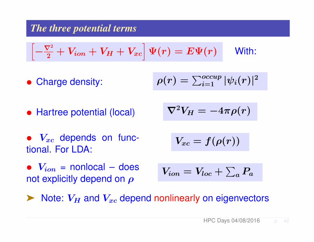
The three potential terms[−∇2
2+ Vion + VH + Vxc
]Ψ(r) = EΨ(r) With:
• Charge density: ρ(r) =∑occupi=1 |ψi(r)|2
• Hartree potential (local) ∇2VH = −4πρ(r)
• Vxc depends on func-tional. For LDA:
Vxc = f(ρ(r))
• Vion = nonlocal – doesnot explicitly depend on ρ
Vion = Vloc +∑aPa
ä Note: VH and Vxc depend nonlinearly on eigenvectors
HPC Days 04/08/2016 p. 42

Self Consistence
ä The potentials and/or charge densities must be self-consistent:Can be viewed as a nonlinear eigenvalue problem. Can besolved using different viewpoints
• Nonlinear eigenvalue problem: Linearize + iterate to self-consistence
• Nonlinear optimization: minimize energy [again linearize +achieve self-consistency]
The two viewpoints are more or less equivalent
ä Preferred approach: Broyden-type quasi-Newton technique
ä Typically, a small number of iterations are required
HPC Days 04/08/2016 p. 43
Self-Consistent Iteration
ä Most time-consuming part = computing eigenvalues / eigen-vectors.
Characteristic : Large number of eigenvalues /-vectors tocompute [occupied states].
ä Self-consistent loop takes a few iterations (say 10 or 20 ineasy cases).
Challenge: Compute a large number of eigenvalues (nev ≈104–105) of a large Hamiltonian matrix (N ≈ 107–108)
HPC Days 04/08/2016 p. 44
PARSEC
ä Represents≈ 15 years of effort bya multidisciplinary teamä Real-space Finite Difference;ä Efficient diagonalization, ...ä Exploits symmetry, ...ä PARSEC Released in∼ 2005.
HPC Days 04/08/2016 p. 45
DIAGONALIZATION: CHEBYSHEV FILTERING

Subspace iteration with Chebyshev filtering
Given a basis [v1, . . . , vm], ’filter’each vector as
vi = pk(A)vi
ä pk = Low deg. polynomial. Enhances wanted eigencompo-nents
The filtering step is not usedto compute eigenvectors ac-curately ä
SCF & diagonalization loopsmergedImportant: convergence stillgood and robust 0 0.5 1 1.5 2
−0.2
0
0.2
0.4
0.6
0.8
1
1.2
Deg. 6 Cheb. polynom., damped interv=[0.2, 2]
HPC Days 04/08/2016 p. 47

Main step:
Previous basis V = [v1, v2, · · · , vm]↓
Filter V = [p(A)v1, p(A)v2, · · · , p(A)vm]↓
Orthogonalize [V,R] = qr(V , 0)
ä The basis V is used to do a Ritz step (basis rotation)
C = V TAV → [U,D] = eig(C)→ V := V ∗ Uä Update charge density using this basis.
ä Update Hamiltonian — repeat
HPC Days 04/08/2016 p. 48
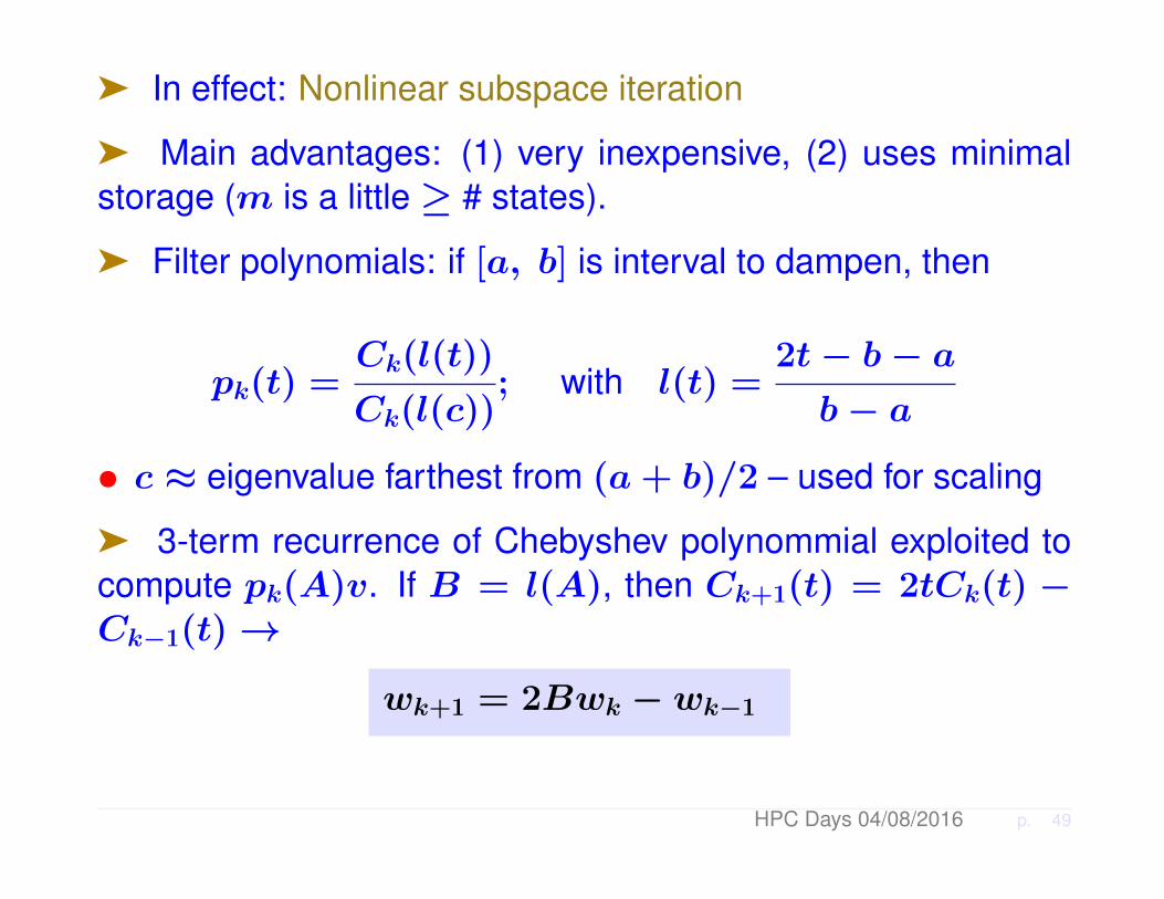
ä In effect: Nonlinear subspace iteration
ä Main advantages: (1) very inexpensive, (2) uses minimalstorage (m is a little≥ # states).
ä Filter polynomials: if [a, b] is interval to dampen, then
pk(t) =Ck(l(t))
Ck(l(c)); with l(t) =
2t− b− ab− a
• c ≈ eigenvalue farthest from (a+ b)/2 – used for scaling
ä 3-term recurrence of Chebyshev polynommial exploited tocompute pk(A)v. If B = l(A), then Ck+1(t) = 2tCk(t) −Ck−1(t)→
wk+1 = 2Bwk − wk−1
HPC Days 04/08/2016 p. 49

Tests with Silicon and Iron clusters (old)
Legend:
•nstate : number of states
•nH : size of Hamiltonian matrix
• # A ∗ x : number of total matrix-vector products
• # SCF : number of iteration steps to reach self-consistency
• total_eVatom
: total energy per atom in electron-volts
• 1st CPU : CPU time for the first step diagonalization
• total CPU : total CPU spent on diagonalizations
Reference: Y. Zhou, Y.S., M. L. Tiago, and J. R. Chelikowsky,Phy. Rev. E, vol. 74, p. 066704 (2006).
HPC Days 04/08/2016 p. 50
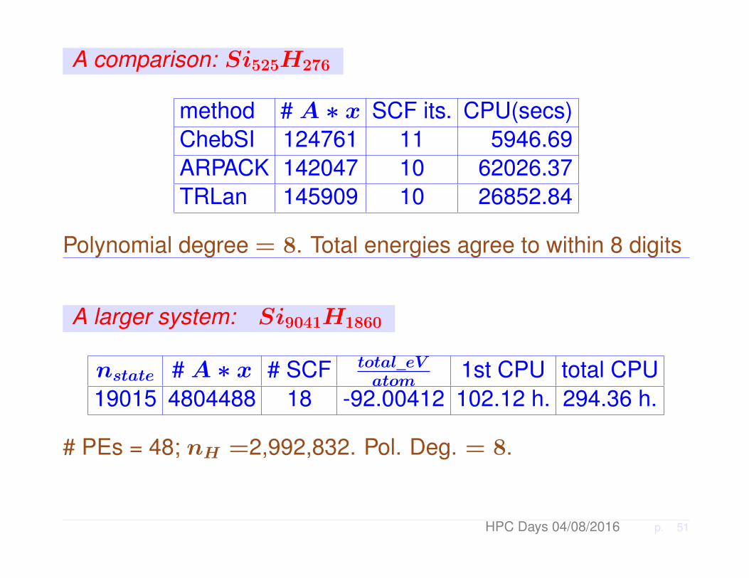
A comparison: Si525H276
method # A ∗ x SCF its. CPU(secs)ChebSI 124761 11 5946.69ARPACK 142047 10 62026.37TRLan 145909 10 26852.84
Polynomial degree = 8. Total energies agree to within 8 digits
A larger system: Si9041H1860
nstate # A ∗ x # SCF total_eVatom
1st CPU total CPU19015 4804488 18 -92.00412 102.12 h. 294.36 h.
# PEs = 48; nH =2,992,832. Pol. Deg. = 8.
HPC Days 04/08/2016 p. 51

Spectrum Slicing and the EVSL project
ä Part of our DOE project on excited states
Conceptually simple idea: cutthe overall interval containingthe spectrum into small sub-intervals and compute eigen-pairs in each sub-interval inde-pendently.Tool: polynomial filtering
−1 −0.8 −0.6 −0.4 −0.2 0 0.2 0.4 0.6 0.8 1−0.2
0
0.2
0.4
0.6
0.8
1
1.2
λφ
( λ )
ä To avoid repeting eigenpairs, keep only the computed eigen-values / vectors that are located in support interval
HPC Days 04/08/2016 p. 52

Levels of parallelism
Sli
ce
1S
lic
e 2
Sli
ce
3
Domain 1
Domain 2
Domain 3
Domain 4
Macro−task 1
The two main levels of parallelism in EVSL
HPC Days 04/08/2016 p. 53

Simple Parallelism: across intervals
ä Use OpenMP to illustrate scaling: Compute 1002 lowesteigenpairs of matrix SiO (n = 33, 401, nnz = 1, 317, 655.)
ä Use 4 and then 10 spec-tral slices
ä Near optimal scaling ob-served as # cores increases
ä Note: 2nd level of paral-lelism [re-orthogonalization+ MatVecs] not exploited.
0 2 4 6 8 10100
200
300
400
500
600
700
800
900
1000
1100Parallel scaling of the divide and conquer strategy
Number of OpenMP threads
Time(sec.)
4 intervals10 intervals
ä Faster solution times with 4 slices (≈ 250 evals per slice)than with 10 slices (≈ 100 evals per slice)
HPC Days 04/08/2016 p. 54

PART 3: DATA MINING
Introduction: a few factoids
ä Data is growing exponentially at an “alarming” rate:
• 90% of data in world today was created in last two years
• Every day, 2.3 Million terabytes (2.3×1018 bytes) created
ä Mixed blessing: Opportunities & big challenges.
ä Trend is re-shaping & energizing many research areas ...
ä ... including my own: numerical linear algebra
HPC Days 04/08/2016 p. 56

Introduction: What is data mining?
Set of methods and tools to extract meaningful informationor patterns from (big) datasets. Broad area : data analysis,machine learning, pattern recognition, information retrieval, ...
ä Tools used: linear algebra; Statistics; Graph theory; Approx-imation theory; Optimization; ...
ä This talk: brief introduction – emphasis on linear algebraviewpoint
ä + our initial work on materials.
ä Focus on “Dimension reduction methods”
HPC Days 04/08/2016 p. 57

Lots of data: can be hugely beneficial (e.g., Health sciences)
HPC Days 04/08/2016 p. 58

Major tool of Data Mining: Dimension reduction
ä Goal is not as much to reduce size (& cost) but to:
• Reduce noise and redundancy in data before performing atask [e.g., classification as in digit/face recognition]
• Discover important ‘features’ or ‘paramaters’
The problem: Given: X = [x1, · · · , xn] ∈ Rm×n, find a
low-dimens. representation Y = [y1, · · · , yn] ∈ Rd×n of X
ä Achieved by a mapping Φ : x ∈ Rm −→ y ∈ Rd so:
φ(xi) = yi, i = 1, · · · , n
HPC Days 04/08/2016 p. 59

m
n
X
Y
x
y
i
id
n
ä Φ may be linear : yi = W>xi , i.e., Y = W>X , ..
ä ... or nonlinear (implicit).
ä Mapping Φ required to: Preserve proximity? Maximizevariance? Preserve a certain graph?
HPC Days 04/08/2016 p. 60
Example: Principal Component Analysis (PCA)
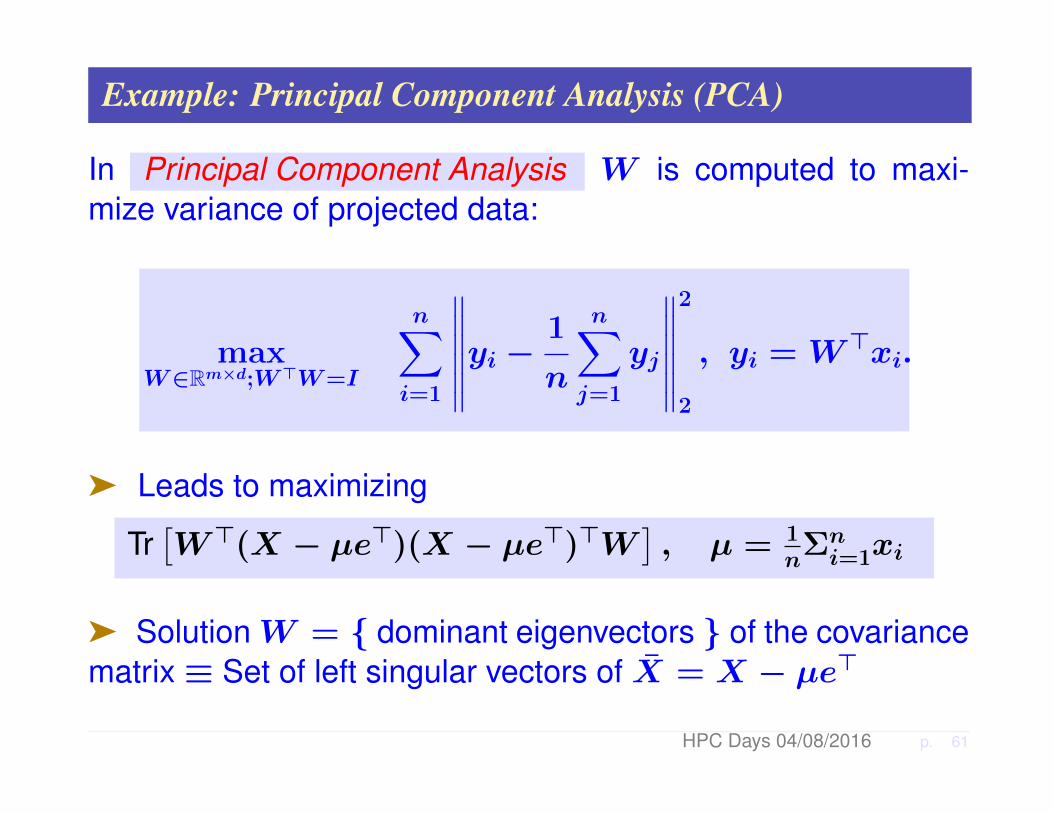
In Principal Component Analysis W is computed to maxi-mize variance of projected data:
maxW∈Rm×d;W>W=I
n∑i=1
∥∥∥∥∥∥yi − 1
n
n∑j=1
yj
∥∥∥∥∥∥2
2
, yi = W>xi.
ä Leads to maximizing
Tr[W>(X − µe>)(X − µe>)>W
], µ = 1
nΣni=1xi
ä SolutionW = dominant eigenvectors of the covariancematrix≡ Set of left singular vectors of X = X − µe>
HPC Days 04/08/2016 p. 61
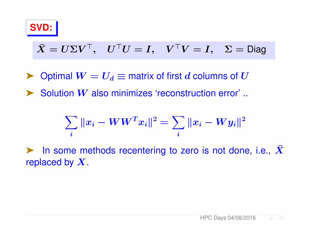
SVD:
X = UΣV >, U>U = I, V >V = I, Σ = Diag
ä Optimal W = Ud ≡ matrix of first d columns of U
ä Solution W also minimizes ‘reconstruction error’ ..
∑i
‖xi −WW Txi‖2 =∑i
‖xi −Wyi‖2
ä In some methods recentering to zero is not done, i.e., Xreplaced by X.
HPC Days 04/08/2016 p. 62

Unsupervised learning
“Unsupervised learning” : meth-ods that do not exploit known labelsä Example of digits: perform a 2-Dprojectionä Images of same digit tend tocluster (more or less)ä Such 2-D representations arepopular for visualizationä Can also try to find natural clus-ters in data, e.g., in materialsä Basic clusterning technique: K-means
−6 −4 −2 0 2 4 6 8−5
−4
−3
−2
−1
0
1
2
3
4
5PCA − digits : 5 −− 7
567
SuperhardPhotovoltaic
Superconductors
Catalytic
Ferromagnetic
Thermo−electricMulti−ferroics
HPC Days 04/08/2016 p. 63
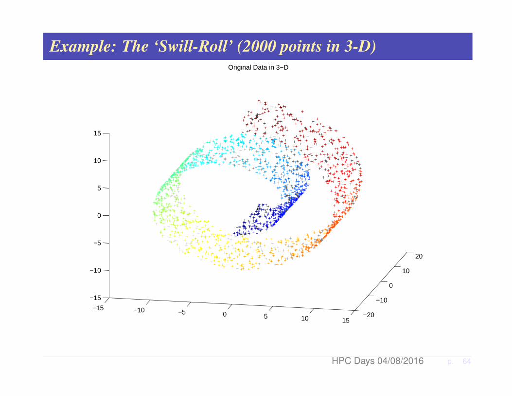
Example: The ‘Swill-Roll’ (2000 points in 3-D)
−15 −10 −5 0 5 10 15−20
−10
0
10
20
−15
−10
−5
0
5
10
15
Original Data in 3−D
HPC Days 04/08/2016 p. 64
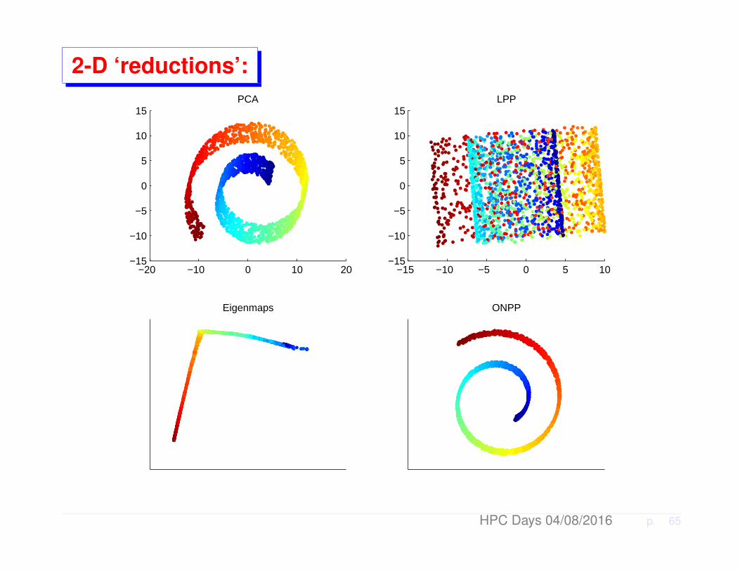
2-D ‘reductions’:
−20 −10 0 10 20−15
−10
−5
0
5
10
15PCA
−15 −10 −5 0 5 10−15
−10
−5
0
5
10
15LPP
Eigenmaps ONPP
HPC Days 04/08/2016 p. 65

Example: Digit images (a random sample of 30)
5 10 15
10
205 10 15
10
205 10 15
10
205 10 15
10
205 10 15
10
205 10 15
10
20
5 10 15
10
205 10 15
10
205 10 15
10
205 10 15
10
205 10 15
10
205 10 15
10
20
5 10 15
10
205 10 15
10
205 10 15
10
205 10 15
10
205 10 15
10
205 10 15
10
20
5 10 15
10
205 10 15
10
205 10 15
10
205 10 15
10
205 10 15
10
205 10 15
10
20
5 10 15
10
205 10 15
10
205 10 15
10
205 10 15
10
205 10 15
10
205 10 15
10
20
HPC Days 04/08/2016 p. 66
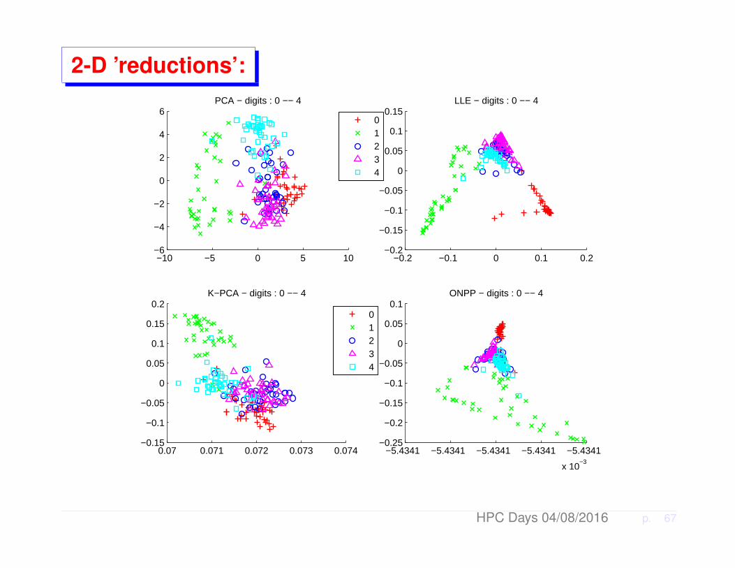
2-D ’reductions’:
−10 −5 0 5 10−6
−4
−2
0
2
4
6PCA − digits : 0 −− 4
01234
−0.2 −0.1 0 0.1 0.2−0.2
−0.15
−0.1
−0.05
0
0.05
0.1
0.15LLE − digits : 0 −− 4
0.07 0.071 0.072 0.073 0.074−0.15
−0.1
−0.05
0
0.05
0.1
0.15
0.2K−PCA − digits : 0 −− 4
01234
−5.4341 −5.4341 −5.4341 −5.4341 −5.4341
x 10−3
−0.25
−0.2
−0.15
−0.1
−0.05
0
0.05
0.1ONPP − digits : 0 −− 4
HPC Days 04/08/2016 p. 67

Supervised learning: classification
Problem: Given labels(say “A” and “B”) for eachitem of a given set, find amechanism to classify anunlabelled item into eitherthe “A” or the “B" class.
?
?ä Many applications.
ä Example: distinguish SPAM and non-SPAM messages
ä Can be extended to more than 2 classes.
HPC Days 04/08/2016 p. 68
Supervised learning: classification
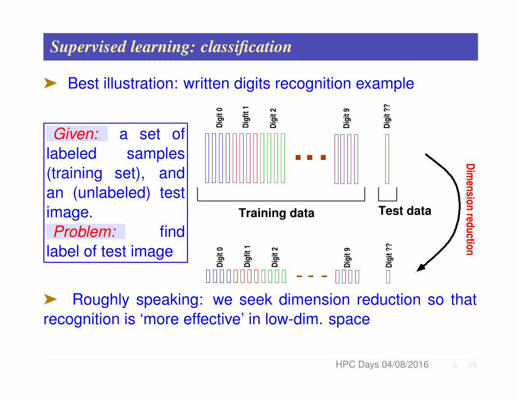
ä Best illustration: written digits recognition example
Given: a set oflabeled samples(training set), andan (unlabeled) testimage.Problem: find
label of test image
Training data Test data
Dim
ensio
n red
uctio
n
Dig
it 0
Dig
fit
1
Dig
it 2
Dig
it 9
Dig
it ?
?
Dig
it 0
Dig
fit
1
Dig
it 2
Dig
it 9
Dig
it ?
?
ä Roughly speaking: we seek dimension reduction so thatrecognition is ‘more effective’ in low-dim. space
HPC Days 04/08/2016 p. 69

Supervised learning: Linear classification
Linear classifiers: Find a hy-perplane which best separatesthe data in classes A and B.
Linear
classifier
ä Note: The world in non-linear. Often this is combined withKernels – amounts to changing the inner product
HPC Days 04/08/2016 p. 70

Face Recognition – background
Problem: We are given a database of images: [arrays of pixelvalues]. And a test (new) image.
↑
?
Question: Does this new image correspond to one of thosein the database?
HPC Days 04/08/2016 p. 71

ä Techniques used in words:
“Build a (linear) projector that does well on some training data.Use that same projector to predict class of new item”
• Some methods use a graph - e.g., neighborhood graph
• Some methods use kernels (change inner products).
HPC Days 04/08/2016 p. 72

Example: Eigenfaces [Turk-Pentland, ’91]
ä Idea identical with the one we saw for digits:
– Consider each picture as a (1-D) column of all pixels– Put together into an arrayA of size #_pixels×#_images.
. . . =⇒ . . .
︸ ︷︷ ︸A
– Do an SVD ofA and perform comparison with any test imagein low-dim. space
– Similar to LSI in spirit – but data is not sparse.
HPC Days 04/08/2016 p. 73

Graph-based methods in a supervised setting
Test: ORL 40 subjects, 10 sample images each – sampleshown earlier # of pixels : 112× 92; TOT. # images : 400
10 20 30 40 50 60 70 80 90 1000.8
0.82
0.84
0.86
0.88
0.9
0.92
0.94
0.96
0.98ORL −− TrainPer−Class=5
onpppcaolpp−Rlaplacefisheronpp−Rolpp
HPC Days 04/08/2016 p. 74

ESTIMATING MATRIX RANKS

What dimension to use?
ä Important question – but a hard one.
ä Often, dimension k is selected in an ad-hoc way.
ä k = intrinsic rank of data.
ä Can we estimate it?
Two scenarios:
1. We know the magnitudeof the noise, say τ . Then,ignore any singular valuebelow τ and count the oth-ers.
2. We have no idea on themagnitude of noise. De-termine a good threshold τto use and count singularvalues > τ .
HPC Days 04/08/2016 p. 76

Use of Density of States [Lin-Lin, Chao Yang, YS]
ä Formally, the Density Of States (DOS) of a matrix A is
φ(t) =1
n
n∑j=1
δ(t− λj),
where• δ is the Dirac δ-function or Dirac distribution• λ1 ≤ λ2 ≤ · · · ≤ λn are the eigenvalues of A
ä Term used by mathematicians: Spectral Density
ä Note: number of eigenvalues in an interval [a, b] is
µ[a,b] =
∫ b
a
∑j
δ(t− λj) dt ≡∫ b
anφ(t)dt .
HPC Days 04/08/2016 p. 77

ä φ(t) == a probability distribution function == probability offinding eigenvalues of A in a given infinitesimal interval near t.
ä In Solid-State physics, λi’s represent single-particle energylevels.
ä So the DOS represents # of levels per unit energy.
ä Many uses in physics
HPC Days 04/08/2016 p. 78

The Kernel Polynomial Method
ä Used by Chemists to calculate the DOS – see Silver andRöder’94 , Wang ’94, Drabold-Sankey’93, + others
ä Basic idea: expand DOS into Chebyshev polynomials
ä Use trace estimators [discovered independently] to get tracesneeded in calculations
ä Assume change of variable done so eigenvalues lie in [−1, 1].
ä Include the weight function in the expansion so expand:
φ(t) =√
1− t2φ(t) =√
1− t2 ×1
n
n∑j=1
δ(t− λj).
Then, (full) expansion is: φ(t) =∑∞k=0µkTk(t).
HPC Days 04/08/2016 p. 79
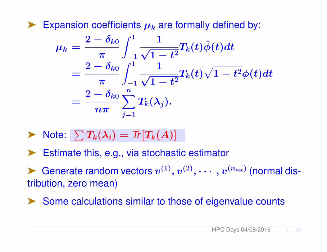
ä Expansion coefficients µk are formally defined by:
µk =2− δk0
π
∫ 1
−1
1√
1− t2Tk(t)φ(t)dt
=2− δk0
π
∫ 1
−1
1√
1− t2Tk(t)
√1− t2φ(t)dt
=2− δk0
nπ
n∑j=1
Tk(λj).
ä Note:∑Tk(λi) = Tr [Tk(A)]
ä Estimate this, e.g., via stochastic estimator
ä Generate random vectors v(1), v(2), · · · , v(nvec) (normal dis-tribution, zero mean)
ä Some calculations similar to those of eigenvalue counts
HPC Days 04/08/2016 p. 80

An example with degree 80 polynomials
0 10 20 300
0.02
0.04
0.06
0.08
0.1
0.12
0.14
0.16
0.18
KPM, deg = 80
t
φ(t)
ExactKPM w/ Jackson
0 10 20 30
0
0.05
0.1
0.15
0.2
KPM, deg = 80
t
φ(t)
ExactKPM w/o Jackson
Left: Jackson damping; right: without Jackson damping.
HPC Days 04/08/2016 p. 81

Integrating to get eigenvalue counts
ä As already mentioned
µ[a,b] =
∫ b
a
∑j
δ(t− λj) dt ≡∫ b
anφ(t)dt
ä If we use KPM to approximate φ(t) = φ(t)/√
1− t2 then
µ[a,b] ≈m∑k=0
µk
∫ b
a
Tk(t)√1− t2
dt
ä A little calculation shows that the result obtained in this wayis identical with that of the eigenvalue count by Cheb expansion
HPC Days 04/08/2016 p. 82
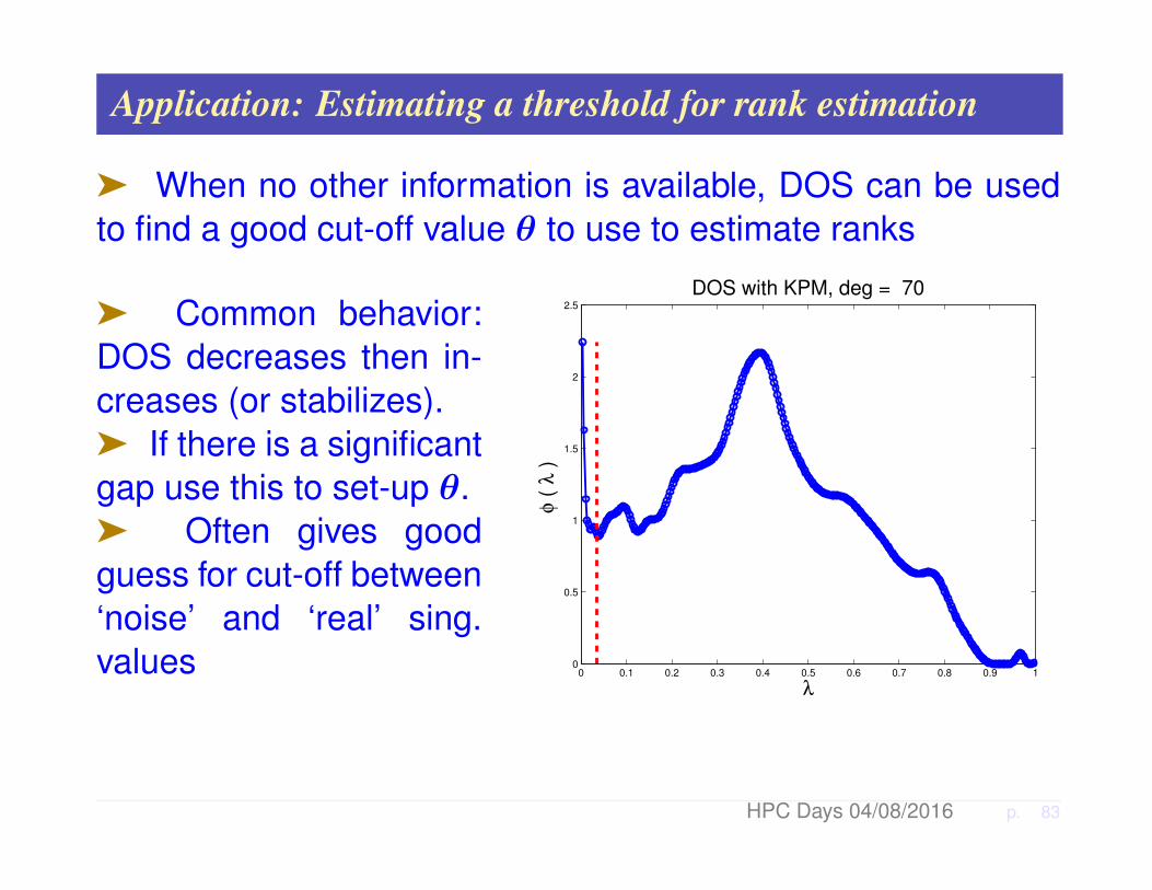
Application: Estimating a threshold for rank estimation
ä When no other information is available, DOS can be usedto find a good cut-off value θ to use to estimate ranks
ä Common behavior:DOS decreases then in-creases (or stabilizes).ä If there is a significantgap use this to set-up θ.ä Often gives goodguess for cut-off between‘noise’ and ‘real’ sing.values 0 0.1 0.2 0.3 0.4 0.5 0.6 0.7 0.8 0.9 1
0
0.5
1
1.5
2
2.5
DOS with KPM, deg = 70
λ
φ (
λ )
HPC Days 04/08/2016 p. 83
Updating the partial SVD
ä In applications, data matrix X often updated
Challenge: Update the partial SVD as fast as possible [e.g.for ‘online’ applications..]
ä Example: Information Retrieval (IR), can add documents,add terms, change weights, ..
ä Methods based on projection techniques – developed in E.Vecharynski and YS’13. Details skipped
HPC Days 04/08/2016 p. 84

MATERIALS INFORMATICS
Data mining for materials: Materials Informatics
Definition: “The application of computational methodologiesto processing and interpreting scientific and engineering dataconcerning materials” [Editors. 2006 MRS bulletin issue onmaterials informatics]
ä Huge potential in exploiting two trends:
1 Improvements in efficiency and capabilities in computa-tional methods for materials
2 Recent progress in data mining techniques
ä Current practice: “One student, one alloy, one PhD” [seespecial MRS issue on materials informatics]→ Slow ..
ä Data Mining: can help speed-up process
HPC Days 04/08/2016 p. 86

Unsupervised learning
ä 1970s: Unsupervisedlearning “by hand”: Findcoordinates that will clus-ter materials according tostructureä 2-D projection fromphysical knowledgeä ‘Anomaly Detection’:helped find that compoundCu F does not exist
see: J. R. Chelikowsky, J. C. Phillips, Phys Rev. B 19 (1978).
HPC Days 04/08/2016 p. 87
Question: Can modern data mining achieve a similar dia-grammatic separation of structures?
ä Should use only information from the two constituent atoms
ä Experiment: 67 binary ‘octets’.
ä Use PCA – exploit only data from 2 constituent atoms:
1. Number of valence electrons;
2. Ionization energies of the s-states of the ion core;
3. Ionization energies of the p-states of the ion core;
4. Radii for the s-states as determined from model potentials;
5. Radii for the p-states as determined from model potentials.
HPC Days 04/08/2016 p. 88

ä Result:
−2 −1 0 1 2 3−2
−1.5
−1
−0.5
0
0.5
1
1.5
2
BN
SiC
MgS
ZnO
MgSe
CuCl
MgTe
CuBr
CuICdTe
AgI
ZWDRZWWR
HPC Days 04/08/2016 p. 89

Supervised learning: classification
Problem: classify an unknown binary compound into itscrystal structure class
ä 55 compounds, 6 crystal structure classesä “leave-one-out” experiment
Case 1: Use features 1:5 for atom A and 2:5 for atom B. Noscaling is applied.
Case 2: Features 2:5 from each atom + scale features 2 to 4by square root of # valence electrons (feature 1)
Case 3: Features 1:5 for atom A and 2:5 for atom B. Scalefeatures 2 and 3 by square root of # valence electrons.
HPC Days 04/08/2016 p. 90

Three methods tested
1. PCA classification. Project and do identification in space ofreduced dimension (Euclidean distance in low-dim space).
2. KNN K-nearest neighbor classification –
3. Orthogonal Neighborhood Preserving Projection (ONPP) - agraph based method - [see Kokiopoulou, YS, 2005]
Recognition rates for 3different methods usingdifferent features
Case KNN ONPP PCACase 1 0.909 0.945 0.945Case 2 0.945 0.945 1.000Case 3 0.945 0.945 0.982
HPC Days 04/08/2016 p. 91
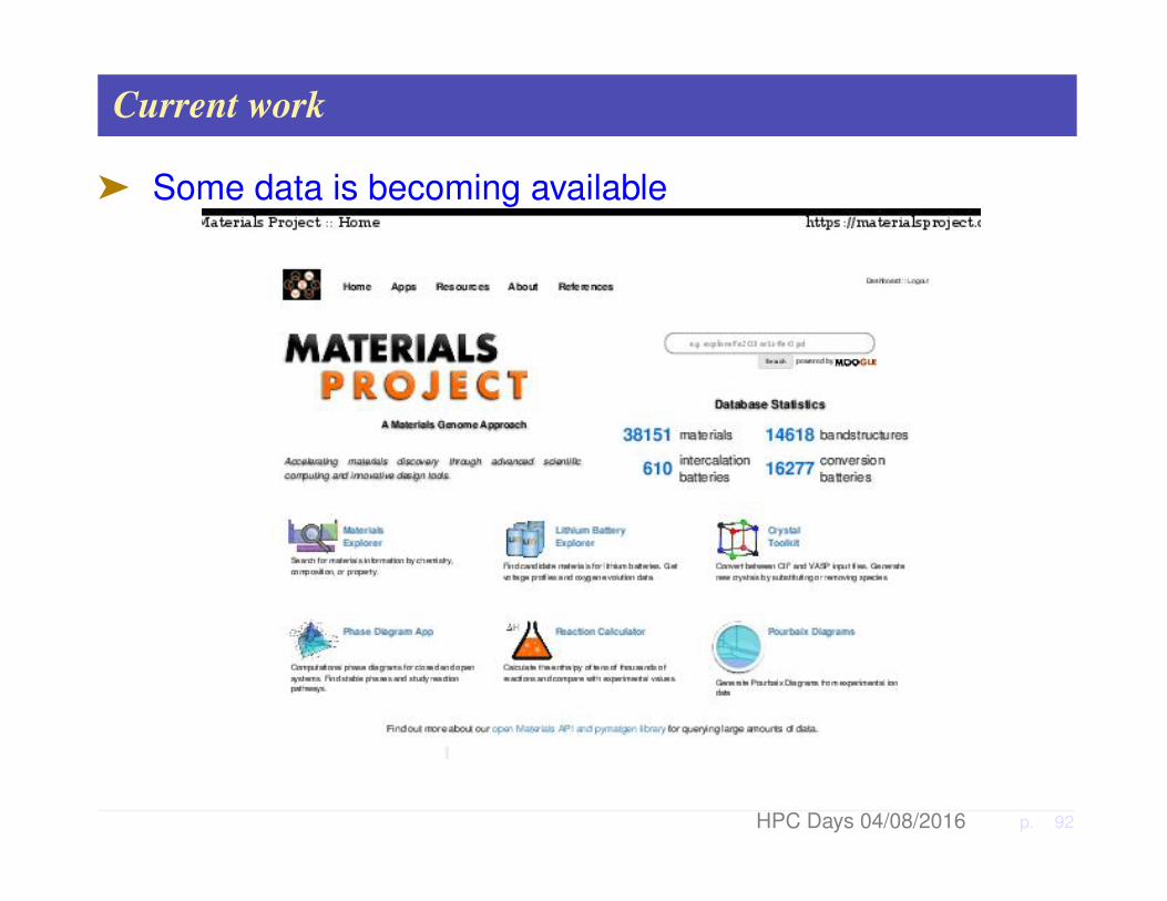
Current work
ä Some data is becoming available
HPC Days 04/08/2016 p. 92
Current work
ä Huge recent increase of interest in the physics/chemstrycommunity
1. Predicting enthalpy of formation for a certain class of com-pounds.. [current]
2. Application to Orthophosphates of lanthanides (LnPO4)[current – with Edoardo di Napoli TRWH]
3. Project: Predict Band-gaps
HPC Days 04/08/2016 p. 93

Conclusion
ä Many, interesting new matrix problems in areas that involvethe effective mining of data
ä Among the most pressing issues is that of reducing compu-tational cost - [SVD, SDP, ..., too costly]
ä Many online resources available
ä Huge potential in areas like materials science though inertiahas to be overcome
ä On the + side: materials genome project is starting to ener-gize the field
ä To a researcher in computational linear algebra : big tide ofchange on types or problems, algorithms, HPC, culture,..
HPC Days 04/08/2016 p. 94
ä But change should be welcome
Two quotes:
“When one door closes, another opens; but weoften look so long and so regretfully upon theclosed door that we do not see the one which hasopened for us.
– Alexander Graham Bell
“Life is like riding a bicycle. To keep your balance,you must keep moving”
– Albert Einsten
HPC Days 04/08/2016 p. 95
![arXiv:0801.1393v1 [cond-mat.mtrl-sci] 9 Jan 2008Turbo charging time-dependent density-functional theory with Lanczos chains Dario Rocca,1,2, Ralph Gebauer,3,2 Yousef Saad,4 and Stefano](https://img.pdfslide.us/doc/110x75/6009348c31591f667f475ee3/arxiv08011393v1-cond-matmtrl-sci-9-jan-2008-turbo-charging-time-dependent-density-functional.jpg)