Policy Research Working Paper 8163

Peer Effects in the Demand for Property Rights

Experimental Evidence from Urban Tanzania

Matthew Collin

Governance Global Practice GroupAugust 2017

WPS8163P

ublic

Dis

clos

ure

Aut

horiz

edP

ublic

Dis

clos

ure

Aut

horiz

edP

ublic

Dis

clos

ure

Aut

horiz

edP

ublic

Dis

clos

ure

Aut

horiz

ed

Produced by the Research Support Team

Abstract

The Policy Research Working Paper Series disseminates the findings of work in progress to encourage the exchange of ideas about development issues. An objective of the series is to get the findings out quickly, even if the presentations are less than fully polished. The papers carry the names of the authors and should be cited accordingly. The findings, interpretations, and conclusions expressed in this paper are entirely those of the authors. They do not necessarily represent the views of the International Bank for Reconstruction and Development/World Bank and its affiliated organizations, or those of the Executive Directors of the World Bank or the governments they represent.

Policy Research Working Paper 8163

This paper is a product of the Governance Global Practice Group. It is part of a larger effort by the World Bank to provide open access to its research and make a contribution to development policy discussions around the world. Policy Research Working Papers are also posted on the Web at http://econ.worldbank.org. The author may be contacted at mcollin@worldbank.org.

This paper investigates the presence of endogenous peer effects in the adoption of formal property rights. Using data from a unique land titling experiment held in an unplanned settlement in Dar es Salaam, the analysis finds a strong, positive impact of neighbor adoption on the household’s choice to purchase a land title. The paper also shows that this relationship holds in a separate, identical experiment held a year later in a nearby community, as well as in admin-istrative data for more than 160,000 land parcels in the

same city. Although the exact channel is undetermined, the evidence points toward complementarities in the reduc-tion in expropriation risk, as peer effects are strongest between households living close to each other and there is some evidence that peer effects are strongest for house-holds most concerned with expropriation. The results show that, within the Tanzanian context, households will rein-force each other’s decisions to enter formal tenure systems.

Peer Effects in the Demand for Property Rights:

Experimental Evidence from Urban Tanzania

Matthew Collin∗†

Keywords: Peer effects, Technology adoption, Land tenure, Tanzania, Unplanned settlements

JEL classification: P14, Q15

∗World Bank; Email: mcollin@worldbank.org†I would like to thank Bet Caeyers, Stefan Dercon, Marcel Fafchamps, James Fenske, and Imran Rasul

for their support, discussions and suggestions, as well as Stefano Cari, Martina Kirchberger, Jan Loeprick,Lara Tobin and participants of the CSAE, DIAL, GREThA, NEUDC conferences and LSE SERC andRockwool seminars for helpful comments and suggestions. I am also indebted to Daniel Ayalew Ali, KlausDeininger, Stefan Dercon, Justin Sandefur and Andrew Zeitlin for their design and implementation of(and my involvement in) the land titling research project from which this analysis was made possible.Finally, I am grateful to Andrew Zeitlin, who provided many helpful thoughts and discussions at the earlystages of the analysis, as well as quick access to some of the administrative data presented in this paper.

1 Introduction

The formalization of property rights is considered by many to be crucial to the institution-al development of societies as well as a path out of poverty for informal property owners(De Soto 2000). Land titling is seen as one of the most fundamental steps in this process,despite mixed evidence of its immediate benefits (Field 2005; Galiani and Schargrodsky2010). While these schemes seem particularly urgent in the face of massive levels of urbangrowth, particularly in Sub-Saharan Africa, very little is known about how to successfullypropagate new tenure regimes.

The context for this paper is Dar es Salaam, which throughout its history has beenshaped by a constant battle between authorities desperate to maintain control over thecity’s development and the ongoing pressure of informal growth and migration from ruralareas. This struggle has roots as far back as the times of British colonial rule, whenthe colonial authorities tried, but largely failed to introduce a formal land title systemto help contain the expansion of a growing Indian population (Brennan 2007). Despitehalf a century of of large-scale urban planning and ‘strict’ government control over theallocation of land, Dar es Salaam remains largely informal today, with over 80% of landbelonging to unplanned, unrecognized settlements (Kombe 2005). It is hardly surprisingthen that the Tanzanian government, like many others dealing with rapid urban growth,has been keen to find innovative ways to sustainably introduce a formal tenure system,both to increase its control over the growth of its urban areas as well as tap into a newbase of revenue.

One facet of both tenure adoption and other formalization decisions that is oftenoverlooked is how individuals’ decisions to enter the formal system might co-vary withone another. Here, I investigate whether the adoption of formal property rights appearsto be contagious, where the action of one agent adopting a new type of tenure increasesthe chance that another does the same. In the peer effects literature these are known asendogenous peer effects (Manski 1993).

The existence of endogenous peer effects in property rights adoption would be mean-ingful for several reasons. First, the existence of adoption spillovers is informative as towhether or not property rights should be considered solely as a private good, or as onewith substantial spatial externalities. Secondly, if the channel through which adoptionpeer effects operate can be identified, we might learn something more about the expectedbenefits of titling. Finally, even if the exact mechanisms remain hidden, the presenceof positive endogenous peer effects is interesting from a policy perspective, as interven-tions aimed at encouraging take up would have a subsequent knock-on effect on others,otherwise known as a social multiplier effect (Glaeser, Scheinkman, and Sacerdote 2003).

Endogenous peer effects are notoriously difficult to identify, as they are subject toboth ‘reflection’ bias (where the direction of causality cannot be determined) and corre-lated effects (where shared unobservable characteristics drives similar decisions). In thispaper, I overcome these standard identification challenges by using exogenous variationin land title purchases resulting from a unique land titling experiment1 in the unplannedsettlements of Dar es Salaam. The experiment randomly allocated a subset of informallandowners to treatment groups which received massive subsidies to obtain a land ti-tle, leaving others excluded. I then combine this variation in the incentive to title withspatial information on the location and treatment status of each household’s set of nearest-neighbors, allowing me to identify the impact of each neighbor’s adoption decision on the

1The experiment is described in detail in Ali, Collin, Deininger, Dercon, Sandefur, and Zeitlin (2016).

2

probability that a given household will purchase a land title. This approach is similar toa number of studies which use randomised selection into a programme to identify peereffects (Duflo and Saez 2003; Lalive and Cattaneo 2009; Bobonis and Finan 2009; Osterand Thornton 2012; Carter, Laajaj, and Yang 2014). These results suggest that there arestrong, positive endogenous peer effects in land title adoption. In my main specification,the probability that a household chooses to purchase a land title increases by 8-15% forevery neighbor that also chooses to purchase one, an effect equivalent in size to a 25-50%discount on the price of the land title. I also show that these results not only diminishwith distance, but they appear to be operating primarily through physical proximity,rather than social proximity, and are not necessarily due to the exchange of information.Furthermore, I show that there is some evidence that households with a higher ex-anteperception of expropriation risk are more responsive to the behavior of their neighbors,suggesting that there are strategic complementarities in adoption to those most fearful ofexpropriation. For robustness, I show that these results hold for some basic changes tothe structure of the peer group. I then go on to show that these results remain roughlyconsistent for an identical experiment rolled out in a neighboring community a year later.Finally, I turn to a database covering roughly 170,000 land parcels in Dar es Salaam,using popular non-experimental methods of identifying peer effects to show that positiveeffects also exist in this larger setting, albeit with a slightly different type of land title.

In the next section, I discuss the setting of urban Tanzania in more detail, as well asthe types of land titles this paper will be covering. Section 3 covers some reasons whypeer effects in land titling take-up are likely to exist. Section 4 outlines the randomisedcontrolled trial which I will exploit to identify peer effects. Section 5 discusses identifi-cation and the empirical set up. Section 6 covers the main results of the paper, Section7 covers the results from the second experiment and administrative data, and I concludewith Section 8.

2 Land tenure in urban Tanzania

In Tanzania, formal access to urban land is controlled exclusively by the government, asall land in the country is owned by the Office of the President (Kironde 1995). Given therates of growth that Tanzania’s cities experienced, the post-independence managementand distribution of urban land has generally been haphazard and insufficient (Kombe2005). Following the 1999 Land Act, the Tanzanian government introduced two new formsof land tenure in urban areas in an attempt to pave the way for more rapid formalizationof existing settlements. The first form of tenure was a temporary, two-year leaseholdknown as a residential license (RL), which had the benefit of being cheap and easy toimplement, but lacked many of the features desired in full titles, such as perpetual security,transferability and collateralizability.

The second form of tenure has been considered to be much closer to a full land title:a certificate of right of occupancy (CRO) lasts 99 years, is transferable and is seen bymany, including providers of credit, as reasonable proof of land ownership. Despite theobvious appeal of the CRO, the Tanzanian government has largely failed to encourageurban land owners to purchase them.2 The lack of progress has been principally due to

2Records from the Kinondoni Municipality in Dar es Salaam indicate that a little over 2,000 applicationsfrom CRO have been made, out of a total population of 60,000 land parcels.

3

the large practical and monetary hurdles that urban landowners face, including expensiveprerequisites such as cadastral surveying and application fees (Collin, Dercon, Nielson,Sandefur, and Zeitlin 2012).

The benefits of CRO ownership

While the Land Act includes relatively straightforward provisions on the legality ofusing CROs to obtain credit or sell land, the interaction between CRO ownership, ex-propriation and compensation is less clear. The Land Acquisition Act of 1967 gives theTanzanian government broad powers to expropriate land for “any public purpose”, evenif the owner is in possession of a CRO. This includes government schemes, general pub-lic use, sanitary improvements, upgrading or planning, developing airfields or ports anduses related to mining or minerals. Indeed, recent history suggests such expropriationseems most likely to occur from government-driven development initiatives (Hooper andOrtolano 2012). While exact figures on government expropriation are not known, thepractice seems frequent enough to elicit alarm in the media: Kironde (2009) found sixexpropriation-related stories in local newspapers in just one week.

While the Tanzanian government is legally obligated to relocate displaced residentsand provide adequate compensation when it acquires land, case studies of recent land con-flicts reveal that these efforts are at best mismanaged and at worst completely neglected(Kombe 2010). While a CRO does not legally protect a household from expropriation, itmight very well indirectly protect a land parcel from government expropriation by raisingthe value of said land and making the compensation transfer more straightforward. TheLand Acquisition Act only provides for compensation in the case where the owner can beidentified (Ndezi 2009). Incidents of government expropriation of urban land reported innewspapers and in case studies suggest that informal settlements face the highest risk, sothere is reason to believe that, when faced with a choice, governments will usually go forthe low-hanging fruit of untitled land.

Even if CRO ownership had no discernable impact on the probability of expropriation,many residents still believe that it does. As part of the baseline data collection forthe experiment used in this paper, residents of two unplanned settlements were askedabout their perceived probability of full expropriation in the next five years. Respondentswere asked to condition their predictions on hypothetically having no title at all, havinga residential license, or having a CRO.3 Figure 1 displays local-polynomial smoothingestimates of the cumulative density function for each response.4 It is clear, at least fora substantial portion of residents, that CROs are perceived to be effective at mitigatingexpropriation risk. As mentioned before, the Land Act also establishes the legal basisfor CROs to be used as collateral for loans. Anecdotal discussions with formal lendersin Dar es Salaam suggests that, while CROs are readily accepted as collateral, they donot necessarily offer a substantial benefit over than of a residential license. Still, evidencefrom the baseline survey used for the experiment described in this paper suggests thathouseholds, on average, also expect that CROs will lead to an increase in both creditsupply and land values. While it is clear that households recognize a private benefit totitling, what this fails to reveal is whether or not landowners perceive any externalities

3The order of the conditional questions were randomized to avoid priming the respondents.4While responses to the expropriation question were discrete bins, differences in perceived risk are

easier to discern using this method. Paired Kolmorogov-Smirnov tests of equality of distributions (notshown) reject the null in every instance.

4

Figure 1: Perceived impact of formal land tenure on expropriation risk

Note: Graph shows local-polynomial smoothed cumulative densities of self-reported perceivedexpropriation probability, conditional on (hypothetical) ownership of different forms of land titles. Datataken from baseline census of landowners in Kigogo Kati and Mburahati Barafu wards in KinondoniMunicipality, Dar es Salaam.

in adoption which would give rise to peer effects, a possibility I will explore further inSection 3.

Before describing the experimental setting where people have been induced to adoptthis new form of land title, I will first consider the reasons why we might expect peereffects in CRO adoption to exist in this context.

3 Peer effects in land rights adoption

Most work on formal property rights bundles the benefits and expected impacts of titlinginto three broad categories, initially summarised by Besley (1995) and later expandedupon in Besley and Ghatak (2010). The first of these is through an (expected) reductionin expropriation risk: formalization should, in theory, reduce the chance a landowner loseshis or her land to either the state or other individuals. In most theoretical contexts, thebenefits of reducing expropriation risk are strictly private and positive. Tenure formal-ization is also expected to make it easier for landowners access credit by giving them theability to collateralize their property. Finally, formalization is expected to increase thetransferability of land, allowing landowners to take advantage of rising land prices andfor ownership to shift to those who can use it most productively.

With the exception of general equilibrium credit market and land price impacts, whichare often ambiguous (Besley and Ghatak 2010), many of these benefits are often modeledas private returns, with the act of one landowner having obtained formal land tenurehaving no impact on other landowners. There are a number of reasons why there mightbe immediate, direct spillovers from the decision to buy a land title, both of which haveimplications for the existence of peer effects. In this section I will consider the most

5

plausible ones, given the context, and then discuss how, in this paper, I will attempt todiscern between them.

Complementarity or substitutability in the returns to land title adoption

One particular area which remains understudied is whether or not there are spilloversin the returns to adopting formal property rights. Individual formalization efforts, such asland titling, might not only result in a private benefit, but might also impact the returnsto titling for other individuals. We might, for example, expect that the returns to titlingwould be increasing in the number of neighbors taking the same action. This is the classiccase of strategic complementarity, when the private returns to an action are greater whenother agents also take it (Schelling 1978; Bulow, Geanakoplos, and Klemperer 1985). Inthe above example, this would be the case when the cross-partial derivative is greaterthan zero, with household i’s returns to titling increasing as more neighbors adopt.

Where might we see strategic complementarities in practice? For one, there might bea snowballing effect in the reduction in expropriation risk, with the government takingformal tenure more seriously as more people adopt it, possibly due to the rising implicitcosts of paying out compensation or because a legal appeal against expropriation is in-creasingly more likely to succeed with each additional titled household. However, even inthe presence of strategic complementarities, expropriation spillovers might not be entirelypositive. If, for example, a government decides to expropriate land which has the lowestlevel of formal tenure, the act of land titling might just shift expropriation risk from oneset of households to another. In this instance, households will be induced to title whentheir neighbors do the same, not because the decision leads to a net gain in welfare, butbecause they must do so to prevent a rise in their risk of expropriation. This impliesthat titling creates a ‘race to the bottom,’ where all households title in order to improvetheir security of tenure, but are no better off at the end of the titling scheme. This resultis akin to De Meza and Gould’s (1992) burglar alarm example: while there is a privatebenefit for a given household installing a burglar alarm, it increases the probability ofneighboring houses being burgled and hence a no-alarm equilibrium is preferable to anall-alarm one.

Complementarities might also exist in the other standard benefits of land titling. Forexample, banks may be more likely to accept land titles as form of collateral if they arewidely used and accepted in a community (Fort, Ruben, and Escobal 2006) or the impactsof titling on land prices might increase as more neighbors adopt.5 In some contexts theformalization of land might also be viewed from the perspective of compliance, whereexpectations of enforcement and social norms can play a roll. Landowners face a similardilemma to that of firms or individual taxpayers deciding to register for or pay tax. Thereis growing evidence that potential taxpayers respond positively the decisions of theirimmediate peers, either because it changes their priors on the probability of enforcementor because it signals a shift in social norms (Chetty 2014; Drago, Mengel, and Traxler2015; Alm, Bloomquist, and McKee 2016).

Of course, titling decisions could also be substitutes: if the marginal utility from titling

5Note that both of these channels might also be subject to net negative impacts. If banks switch to aregime where formal titles are the only legitimate form of collateral, non-adopting households might berationed out of the market (Van Tassel (2004) shows a similar result might happen even if all householdsare given title. Similarly, if titles become the de facto means of transferring property, households relyingon informal channels may feel the need to adopt if they are to sell in the future.

6

decreases as more neighbors take up, then household i will be more likely to opt out.6

If the main benefits of titling are through reducing expropriation risk, this would reflecta context where low levels of titling are enough to deter a government from clearing anarea, and so subsequent titling is less effective. Similarly, some have argued that thecredit-supply effects of large scale titling will be smaller than individual titling: if lendersconsider titling to be a signal of borrower quality, rather than as a collateralizable asset,then large-scale titling would imply a lower signal-to-noise ratio (Dower and Potamites2012).

Strategic complementarity (substitutability) in the returns to titling would imply apositive (negative) endogenous peer effect, as the effect of neighbor take-up increases (de-creases) the marginal benefit to titling for a given household. For most of the impactsdiscussed here, we would also expect these spillovers to be inherently spatial: both ex-propriation risk and land values are typically highly correlated across space (as might becollateral values, as lenders might be more confident in extending loans to areas they arealready familiar with). Later on on this paper, I will take advantage of the spatial natureof the data to discern whether or not the observed endogenous peer effect varies withdistance.

Learning and rule-of-thumb behavior

Peer effects might also arise from learning behavior: based on their peers’ experience,individuals update their beliefs on the efficacy of a product. This ‘social learning’ behaviorhas already been revealed in the decision of farmers to adopt new farming techniques ornew types of crops (Bandiera and Rasul 2006; Conley and Udry 2010; Zeitlin 2012). Thiscould equally apply to landowners in urban areas who observe their neighbors obtainingland titles and possibly being secure from expropriation, gaining access to credit or sellingat a high price. Yet, in the context of this study, the benefits of holding a land title wouldbe impossible to measure: as I will discuss in the next section, land titles were ultimatelynot issued for landowners involved in the field experiment. This prevents the sort ofwait-and-see learning observed in previous studies.

However, if landowners believe that the adoption decisions of their peers reveal theirknowledge about the benefits of land titling, high rates of peer adoption may act as asignal for high returns. Recent evidence suggest that peers’ adoption decisions transmitimportant information, irrespective of actual adoption outcomes (Bursztyn et al. 2014).In this circumstance, any observed endogenous peer effects would be unambiguously pos-itive, as take-up conveys a signal of high-returns to titling.

It is normally difficult to disentangle peer effects created by strategic complementari-ties from signaling/learning behavior. However, we might expect peer effects determinedby the latter to transmit through traditional social networks, as households observe thebehavior of not only their neighbors, but also their friends and acquaintances. Later inthis paper, after establishing that that endogenous peer effects in land title take-up existbetween spatially-proximate households, I will then take advantage of some basic socialnetwork data to investigate whether or not endogenous peer effects also exist across thisalternate network structure, which would suggest that effects other than complementari-ty/substitutability spillovers are at play.

6This opens the door for standard public goods/collective action problems, as everyone has a privateincentive to disinvest if they know their neighbor is investing.

7

Other channels

Another concern might be strategic expropriation on the part of those obtaining aland title, with early-movers grabbing a portion of their neighbor’s land by making anearly claim. While this might be a concern in other settings, it is unlikely to be a factorhere, as contiguous neighbors must sign off on the CRO application forms affirming theboundaries of the plot. Furthermore, these sorts of actions would still fall under the‘complementarity’ channel: if adopting a CRO protects me from my neighbor’s attemptto grab land, my neighbor’s action increases the marginal gain from adopting that title.

Finally, there might be information-transfer peer effects, where households learn aboutthe benefits of CRO adoption and share this information, then make entirely independentdecisions to title. I will discuss this channel and my attempt to rule it out more in thenext section.

4 Experimental design and data collection

As I described in the Section 2, most households in Dar es Salaam face formidable barriersto the adoption of formal land titles. In this section, I will describe an experimentally-provided land titling program designed to overcome these barriers. The experiment,conceived as part of an impact evaluation of CRO adoption, is described in detail inAli, Collin, Deininger, Dercon, Sandefur, and Zeitlin (2016). The random variation inCRO adoption induced by the experiment will then be used to identify the impact of aneighbor’s adoption on a given household’s propensity to adopt.

4.1 An experimental land titling program

The setting is Kinondoni, which is the largest of the three municipalities which make upDar es Salaam and houses approximately 50% of the city’s population. The land titlingprogram was introduced in two adjacent neighborhoods (known as sub-wards or mitaa),first in Mburahati Barafu then a year later in Kigogo Kati. Barafu will be the main focusof this paper, due to the completeness and robustness of its data, although I will be usingthe subsequent replication in Kati as a robustness check in Section 7.1.

Both neighborhoods are located approximately five kilometers from the city center.While there are a number of pre-planned parcels at the core of each settlement, each mtaais primarily composed of unplanned, informal settlements. Table 1 displays some basicadministrative data from both neighborhoods alongside Kinondoni as a whole. Typical ofmost informal settlements, Barafu is a high density area with relatively low reported landvalues and a lack of access to public services and infrastructure. Informality is the normhere, with very few households holding formal tenure: estimates from a baseline censusof Barafu put the total number of CRO owners at around 10 households, less than 1% ofthe community, and administrative data suggests less than 40% of households have everpurchased a residential license.

In October, 2010, the University of Oxford and the World Bank began implementinga land titling program ultimately aimed at identifying the impact of CRO adoption inBarafu. This was done in partnership with the Woman’s Advancement Trust (WAT),a Tanzanian NGO which specializes in large-scale titling programs. The interventionproceeded as follows: prior to launching the land titling program, all land parcels inBarafu were identified via a household listing of the community and a recent map drawn

8

Table 1: Summary Statistics on Parcel Characteristics

Kinondoni Kigogo MburahatiMunicipality Kati Barafu

Formal employment 49.9% 44.6% 44.3%Size and Value of Property

Area in square meters 439 264 247Property value in ’000 TSh. 12,562 9,939 8,910Land rent in TSh. 3,679 2,125 1,907

Accessibility to the PropertyNo access 1.3% 1.1% 1.1%Foot path 55.2% 71.3% 82.0%Feeder road 36.4% 19.8% 16.2%Main road 5.5% 6.6% 0.6%Highway 1.6% 1.1% 0.0%

Access to Public UtilitiesPiped water (incl. public) 22.7% 22.0% 5.6%Electricity connection 46.1% 38.6% 35.1%

Waste removal servicesBurn/buried on plot 35.4% 25.4% 55.7%Gutter/river/street 20.0% 49.6% 35.4%Collected by priv. company 40.8% 24.4% 8.4%Collected by municipality 3.8% 0.7% 0.5%

Number of properties 65,535 1,474 990

Source: Author’s calculations based on the land registry maintained by Kinondoni Municipality.

up by a town-planning firm. This map was used to divide the community up into 20‘blocks’ of roughly 40-50 parcels each. Using a set of basic characteristics taken fromthe listing to establish balance, 10 blocks were randomly allocated to a treatment groupand ten to a control group. Balance results for the overall treatment are available inTable 12 in Appendix A.1. Figure 2 shows the map of Barafu with treatment and controlblocks outlined. Parcels in treatment blocks (and their owners) were subject to severalinterventions:

1. All parcels in treatment blocks were subject to a cadastral survey (demarcation ofboundaries using cement beacons), one of the prerequisites for applying for a CRO.

2. Parcels in treatment blocks were invited to meetings to discuss involvement in theland titling program and the benefits of CRO ownership, run by WAT.

3. During these meetings and subsequent follow-up visits, treatment parcels were invit-ed to pay 100,000 TSh to WAT (approximately $62, the average cost of the cadastralsurveying plus application fees) over a period of about five months in return for aCRO. In exchange for this, WAT would manage the application process and anyrelated fees.

4. Within treatment blocks, parcels were randomly allocated voucher discounts througha public lottery. Two types of vouchers were allocated: general vouchers, which wereredeemable without condition, and conditional vouchers, which required that a fe-male member of the household be included as an owner on the final documents. Aparcel could receive both voucher types, just one type, or none at all, and vouchers

9

Figure 2: Treatment and control blocks in Mburahati Barafu

Note: Treatment blocks are shaded grey.

could take on values of 20, 40, 60 or 80 thousand shillings.7

Following this, households in treatment blocks were free to sign up and begin repay-ment. Through an agreement with the municipal government, treated households couldnot obtain a CRO through conventional means, only through the NGO. Households incontrol blocks were free to obtain CROs through the municipality, at the regular cost,although a subsequent review of municipal records revealed that none have done so todate.

The project began in late 2010 and repayment in both subwards took place throughout2011 and much of 2012. However, following this initial repayment period, the Tanzaniangovernment made a number of decisions which prevented CROs from being issued tothe residents of the study area. After Dar es Salaam was subject to a high degree offlooding in late 2011, the Ministry of Lands decided to classify a large proportion of thestudy area as being ineligible to be covered by a CRO due to its proximity to low-lying,flood prone areas of the city. This, combined with the Ministry’s decision to drastically(and unexpectedly) raise the price of obtaining a CRO, led to substantial delays in theprocessing of CROs. Ultimately, in 2015 the project determined it would not be able toguarantee that households in the community would be able to receive a CRO and insteadoffered residents the option to have their contributions refunded with interest.

Despite the fact that the project was ultimately unsuccessful, the payments made byresidents of Mburahati Barafu and Kigogo Kati during the first two years of the projectrepresent concrete, credible decisions made at a time when the project did appear tobe moving forward. As is described in more detail in Ali et al. (2016), there was noexpectation by either the residents, the participating NGO or the researchers that theproject would fail.

7Complete details of the voucher allocation process are discussed in Ali et al. (2016)

10

4.2 Data sources

In this paper I use three primary sources of data from Barafu. The first was collected priorto the randomised intervention: in the summer of 2010, roughly six months before thestart of the land titling program, the University of Oxford conducted a complete census ofall known parcels in Barafu, using records obtained from the Kinondoni Municipality. Foreach parcel, an owning household was identified and interviewed, resulting in a rich dataset of owner and parcel characteristics. However, as this data was collected earlier andused a different sample frame than the administrative project data, there are a number ofmissing observations, mainly due to parcels which were missed during the baseline censusor those that were sold to a new owner in the interim. Baseline data are available forroughly 92% of unplanned parcels in treatment blocks, but only 72% of control blockshave linked baseline data, due to a lack of project information for these households. I willuse these data both for testing balance and for controls in my main specification.

The second is detailed parcel-level data taken from project records, including meetingattendance, sign-up and repayment information. As households in control blocks wereexcluded from participating in the project, this data only contains information on treatedparcels. However, data obtained from the Kinondoni municipality reveals that no parcelsin the control blacks purchased a CRO during the time frame of the project. Finally, thethird source of data I use is detailed geographic information service (GIS) encoded dataon the location, shape and size of each parcel in both treatment and control areas.8 Thiswill allow me to calculate ‘nearest-neighbor’ peer groups for every parcel and compare theprobability of a household choosing to purchase a CRO with the average adoption rate ofthat household’s nearest-neighbor set.

Throughout the remainder of the paper, I will primarily be using unplanned parcelsin the analysis, as this group was the original target of the research. While there iscomplete project data and limited baseline data on planned parcels (those who were in apre-planned area or had already obtained a cadastral survey prior to the intervention), Iwill only be using them as a robustness check for the main result.

5 Identification of peer effects

Consider a basic linear probability model for household i’s decision to adopt a land title:

Ti = α+ ρT g(−i) + xiβ + xg(−i)δ + ui + εg + εi (1)

Where Ti is the household’s choice to adopt a land title, T g(−i) is the average choice of thehouseholds group of neighbors g (excluding i), xi is a vector of household characteristics,xg(−i) is the same set averaged over the group, ui is a household-specific effect and εg is avector of group-specific characteristics. Using Manski’s (1993) terminology, ρ is known asthe endogenous effect, the impact of i’s neighbors’ choices on i’s choice. The parameterδ represents a vector of effects stemming from i’s neighbors’ characteristics, known asexogenous or contextual effects. Finally, εg contains unobserved within-group correlatedeffects.

There are two primary challenges to the identification of ρ, the parameter of interest.

8This data was taken from a ‘town plan’ of Barafu, the final planning document drawn up for acommunity before CROs can be provided

11

The first is a result of Manski’s ‘reflection problem’, where the direction of causality isdifficult to discern. At first glance, we are unable to identify whether ρ captures aggregateeffects of i’s neighbors’ adoption on i or vice versa. In the extreme case where peer groupsare perfectly transitive,9 it is difficult to separately identify endogenous peer effects ρ andthe set of contextual effects δg.10 However, when peer or neighbor groups are partiallyoverlapping (i.e. when the neighbors of i’s neighbors can reasonably be excluded fromi’s neighbor set) identification is made possible by exploiting variation in characteristicsof these excluded neighbors (Bramoulle et al. 2009; De Giorgi et al. 2010), a popularmethod I will apply to a larger, non-experimental data set in Section 7.2.

The second concern is over conflating endogenous peer effects with correlated effects.The latter can arise when peer groups or neighbors are affected by common backgroundcharacteristics or shocks which also predict adoption. For example, if land title adop-tion depends on unobserved (to the researcher) land quality, then adoption rates will becorrelated across neighbors even in the absence of endogenous effects. Similarly, if theendogenous sorting of households into peer groups or neighbor sets is marked by homophi-ly, then correlated adoption decisions might solely be the result of correlated individualcharacteristics, such as wealth or risk aversion.

In this paper, I use the random variation in the price and accessability of land titlepurchase to identify exogenous changes in Tg(−i), allowing me to estimate (1) using two-stage least squares (2SLS) with reduced concerns for correlated effects and reflection. I dothis using the percentage of household i’s neighbors who were included in treatment blocksas well as their average voucher values11 as instruments for the average adoption of theneighbor set. Since households in control blocks were effectively excluded from purchasingCROs, the sample will only cover households in treated blocks (although I will considerneighbors from both treatment and control blocks). I will discuss the suitability of theseinstruments and possible reasons why identification might still fail in the next subsection.

While many studies have used random variation in group assignment to estimate peereffects (Sacerdote 2001; Guryan, Kroft, and Notowidigdo 2009), my approach in thispaper is more similar to those which use random variation in program assignment as aninstrument for peer-level adoption. For example, both Lalive and Cattaneo (2009) andBobonis and Finan (2009) use the random assignment of a conditional cash subsidy inPROGRESA villages to instrument for the school enrollment of a child’s peer group.Similarly, Oster and Thornton (2012) use the random assignment of menstrual pads toNepalese school girls to study the impact of group-level treatment on individual utilizationof the pads. Both Godlonton and Thornton (2012) and Ngatia (2011) use randomizedprice incentives to get tested for HIV/AIDS in Malawi to instrument for peer grouptesting. In each of these studies, social interactions are treated as a specific type oftreatment spillover: an individual’s peer group is randomly shocked and the resultingchange in behavior affects the individual’s adoption choice. This method was first laidout by Robert Moffitt as the partial-population approach (Moffitt et al. 2001).

There are a couple of caveats to the interpretation of ρ using the partial-populationapproach. First, while properly instrumenting Tg(−i) solves the reflection problem andbypasses any group or individual-level unobservables, the resulting estimate of ρ is the

9Transitivity implies that if i and j are peers and j and k are peers, then i and k must also be peers.10Brock and Durlauf (2001) exploit nonlinearities in discrete choice models to identify linear-in-means

models, yet identifying assumptions are heavily dependent on functional form, and do not allow forcorrelated effects.

11Averaged over included-neighbors. For precision I use both regular and conditional vouchers sepa-rately.

12

endogenous peer effect, conditional on groups already having formed endogenously. These‘true’ peer effects might be stronger or weaker for households which have chosen to livetogether as opposed to those randomly sorted into the same neighborhood. For instance,households from the same religious background might be more likely to associate and shareinformation about adoption decisions. In this instance, we might expect the estimate ofρ, post-endogenous sorting, to be higher than the estimate under random sorting.

Which estimate do we care about? While the ‘randomly-assigned’ endogenous peereffect might be more appealing to those concerned with pure social interactions, in realitythe policy maker has little control over the formation of these peer groups, in whichcase the ‘post-sorting’ endogenous peer effect is clearly the preferred parameter. In thecontext of urban formalization, most policy makers are burdened with the significanttask of getting large, informal settlements to take up formal property rights. As thesesettlements have not formed randomly, the post-sorting peer effect gives us an idea as towhether significant policy multipliers are present for property rights interventions.

Another issue follows directly from using 2SLS with an exogenous treatment instru-ment to identify peer effects. Under the assumption of heterogenous effects, instrumentalvariables regressions only allow the researcher to identify the local average treatmenteffect (LATE) (Imbens and Angrist 1994). The implications of this for the estimationof peer effects are nonnegligible. For example, when using the block-level treatment asan instrument for neighbor adoption, the effect identified ρ is only defined for complier-s, households whose neighbors were induced to adopt from the treatment, but otherwisewould have not done so. As mentioned in the previous section, there are no always-takers,so estimates of ρ using project treatment of an instrument will only be leaving out never-takers, those that do not respond to the treatment. If we have reason to believe that peereffects are heterogenous, then LATE estimates of ρ might deviate substantially from theaverage treatment effect estimate. The peer effects literature has largely been silent onthis issue, with some exceptions.12

Finally, it should be emphasized that while the randomized control trial describedabove has generated geographic variation in the take-up of CROs, the block-level RCTitself was not designed for the purpose of of studying peer effects. Thus most13 of theidentifying variation in take-up will be generated by the large-scale block-level variationin treatment. While this is not as precise as a parcel-level treatment, identification willbe possible as long as treated neighbors are not systematically different from untreatedneighbors or households with treated neighbors are systematically different than thosewithout. To allay any concerns, I will show in Section 5.2 that when compared usingbaseline data, treated and untreated parcels are, on the whole, very similar.

5.1 Challenges to identification

Even though the instruments I use in this paper are randomly drawn, there are still anumber of ways the above identification strategy might be undermined. For instance,despite the randomization, a bad draw in assignment of treatment status or voucher val-ues might have resulted in spurious correlation with relevant unobservable characteristics.Later, I will show that not only both treatment and voucher assignment are well-balanced

12To date, only Dahl, Løken, and Mogstad (2014) and Ngatia (2011) have explicitly acknowledged thatpeer effects estimated using 2SLS are subject to a LATE interpretation. Ngatia (2011) explicitly modelsthese heterogenous effects and estimates their effects by exploiting multiple instruments for adoption.

13Some of the variation will still be driven by variation in the voucher allocation received by treatedneighbors.

13

across a range of observable characteristics obtained from the baseline census, but thatthe main results presented in Section 6, are unaffected by the inclusion of these character-istics. While balance and conditioning on observables does not guarantee identification(Bruhn and McKenzie 2009), randomization is as close as we are ever likely to get, asin expectation the instruments should be uncorrelated with the error term in the mainequation.

A more pertinent problem is the exclusion restriction. In order for the estimate of ρ tobe interpreted solely as an endogenous peer effect, the instruments (being in a treatmentblock and the random voucher draw) must only affect a household’s adoption of a landtitle through the adoption of its neighbors. There are a few reasons why this might notbe the case:

One valid concern is that direct-adoption peer effects might be confused with infor-mation exchange. Prior to the intervention, most residents knew very little about CROs.Since households in treated blocks are invited to meetings in which they are given exten-sive information on the benefits of these titles, it is possible that attending householdspassed this information on to their non-attending neighbors. Thus the observed peer ef-fect ρ might include the impact of this information transfer. To account for informationin my main specification, I will use data on household and neighbor meeting attendanceto proxy for knowledge of CROs.

Another potential problem is related to a second change in neighbor characteristicsdriven by the treatment. Recall that all parcels in treatment blocks are subject to acadastral survey, even if the owners do not go on to purchase a land title. The act ofsurveying a neighbor’s plot could have an independent effect on a household’s decisionto purchase a CRO if, for instance, being in a heavily-surveyed area affects the perceivedvalue of a title. Recent evidence suggests that land demarcation has important impli-cations for the function and growth of land markets (Libecap and Lueck 2011), so it ispossible that a shift from the previous regime14 to tightly-regulated cadastral surveyingcould have substantial impacts independent of land title adoption.

To deal with this, I first turn to data from the baseline census, which suggests that ahousehold’s perceived expropriation risk is unaffected by proximity to previously-surveyedparcels. Secondly, I also find that endogenous peer effects are of a similar magnitude whenI include previous-surveyed parcels as neighbors.15 Finally, the timing of the interventionsuggests that adoption decisions might have been independent of surveying: while treat-ment and control blocks were decided at the beginning, actual cadastral surveying did notbegin until several months following the initial sign-up period, and took over a year tocomplete, so the final surveying status of treated-neighbors would have been unconfirmedfor most households.

Another assumption behind the exclusion restriction is that proximate neighbors haveindependent budget constraints. This would be undermined if two neighbors act as a singlehousehold or take part in risk-sharing groups.16 However, while spontaneous risk-sharinggroups have been observed in randomized controlled trials in the past,17 the chances of

14Prior to the introduction of the town plan, parcels were delineated with hand-drawn maps producedusing aerial photography.

15Both of these results are available upon request.16Lalive and Cattaneo (2009) discuss this as a potential threat to identification, where sharing of

PROGRESA transfers might lead to a spurious social interaction result.17 Blattman (2011) discusses difficulties with lottery recipients exchanging winnings. Similarly An-

gelucci and De Giorgi (2009) shows that ineligible households are affected by cash transfers to treatmenthouseholds.

14

such an arrangement existing in this context are slim, given that the households werepresented with non-transferable vouchers which were tied to individual parcels.

Finally, the exclusion restriction might be undermined if households decide not toparticipate in the program because of concerns for fairness (for their neighbors not beingincluded) or if high/low voucher allocations to neighbors elicit feelings of envy or unfair-ness which stop them from adopting. However, anecdotally there is not much evidencethat these sort of feelings are at play on the ground.

5.2 Empirical setup

Reconsider the empirical model presented in equation (1), which is presented as a linearprobability model (LPM):

Ti = α+ ρT g(−i) + xiβ + xg(−i)δ + ui + εg + εi

While it is possible to estimate this using a nonlinear specification, such as a probit orlogit, the LPM makes interpretation of the results relatively straightforward. The chiefconcern over the use of a LPM is over out-of-sample predictions and the potential biaswhich results from its use. In Table 17 in Appendix A.1, I show that the percentage ofout-of-sample predictions is extremely low, which suggests that there is not much scopefor bias in the LPM (Horrace and Oaxaca 2006).

A dummy variable equal to one if a household has fully paid for its CRO will beused as my main measure of title adoption Ti.

18 In my main specification, for house-hold/parcel characteristics xi, I will include the general and conditional voucher valuesthat the household received and a control for whether or not that household attended theblock-level meeting. In addition, I will include a series of baseline controls, including thenatural log of the parcel’s area, the year the parcel was obtained, the household’s monthlyincome, total value of all assets (TSh), household size, average schooling and dummy vari-ables for whether the parcel is rented out, the owner is resident on the parcel, and therehas been recent investment in the parcel. Each of these controls is also averaged acrossthe household’s neighbor set and included in xg(−i), with the exception of the neighbor’svoucher values, which are used as instruments. I have also included a control for whetheror not the household has neighbors outside of the treatment block, so as not to conflatedifferences in neighbor treatment with the household’s relative location within the block.

Using GIS data to calculate distances between parcel borders, I construct peer groupsusing the n closest neighbors to household i. This approach allows for results whichare intuitive and easy to understand, as each house has equal-sized peer groups. Forrobustness, I will also present results using fixed-distance neighbor sets (which includeall neighbors within a certain distance d), but the differences are minor. As it offersa reasonable trade-off between proximity and the power of the instruments,19 my mainresults will use the five nearest-neighbors, but extensions on the size of the neighbor setsare presented in Section 6.2.

Summary statistics for the main controls, as well as their balance across voucherallocations and the percentage of five nearest-neighbors treated, are shown in Table 2.Parcels which faced a high price were slightly less likely to be electrified and had slightlyhigher levels of schooling, but neither of these differences are substantial. Households with

18Results are also robust to using household sign-up as a measure of adoption instead of full purchase.19The larger the neighbor set the greater the number of households which fall outside i’s block and

therefore have the potential to be treated.

15

a high percentage of treated neighbors were more likely to attend meetings and were lesslikely to have purchased a residential license. Apart from these differences, the sampleappears to be fairly well-balanced.

Finally, I will be using both average voucher values across the neighbor set and thepercentage of treated neighbors as instruments for T g(−i). While the results are robustto including these as separate instruments, the estimates are most precise when they areaggregated into a single instrument. This instrument is defined as the ‘total’ price of aCRO per household, which is set to TSh 500,000 for untreated neighbors (which is in linewith previous estimates)20 and set to the actual project price, net of vouchers, for treatedneighbors.

To account for spatial dependence of observations, all standard errors are calculatedusing Conley’s (1999) method, where the estimated covariance matrix is adjusted toallow for arbitrary spatial correlation between observations. The degree of correlation isallowed to decrease linearly with distance and is set at zero beyond a specified cutoff. Forall nearest-neighbor specifications, cutoff values are set at the average distance of the fifthneighbor across observations. For distance-band specifications, cutoff values are set equalto the distance-band. In general, the results are not qualitatively different from standardheteroskedastic-robust estimates.

6 Main results

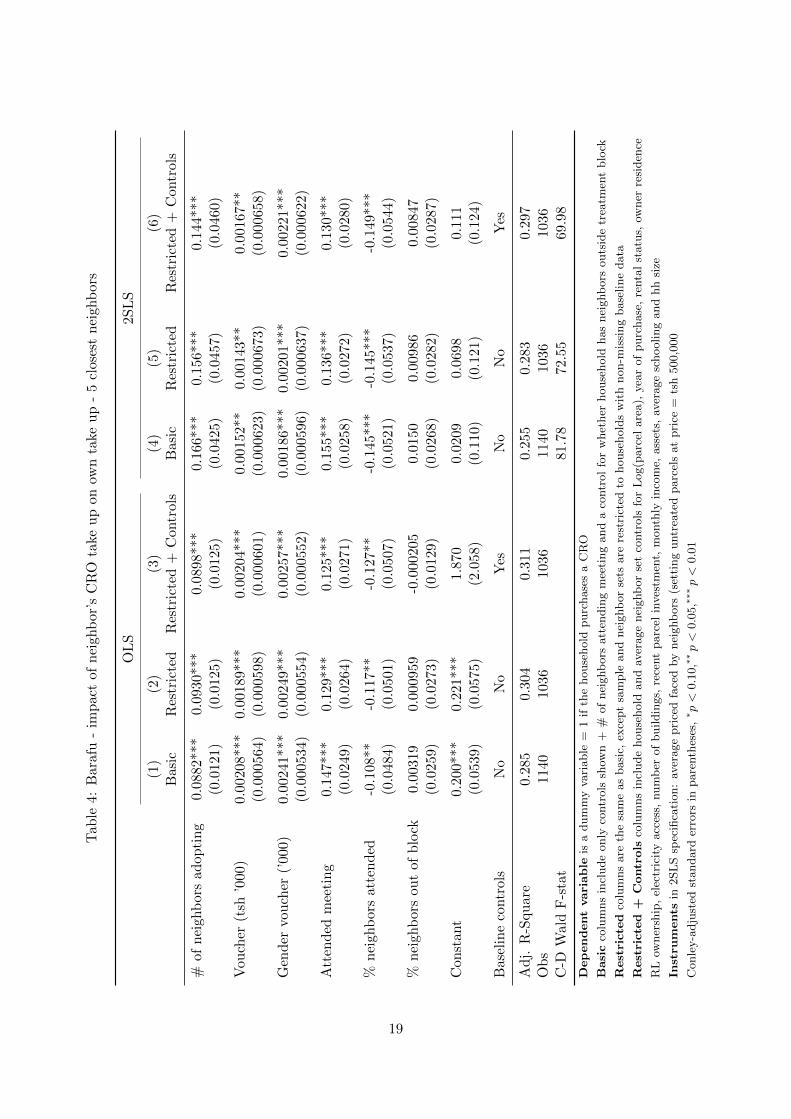
Table 4 shows the results from the estimation of equation (1) using the five nearest-neighbors as the relevant peer group. The first three columns display results from anOLS estimation of the probability that household i adopts a land title on the number ofneighbors in the neighbor set also adopting.21 In column (1), the controls included arehousehold i’s allocated vouchers, whether or not someone from the household attendedthe information/voucher distribution meeting held for the treatment block, the percentageof i’s neighbors who attended a meeting and the percentage of neighbors who are in adifferent treatment/control block. Column (2) restricts the sample to households withbaseline data and the nearest-neighbor set to neighbors with baseline data, but doesnot include baseline controls. These are introduced in column (3), so as not to conflatesample-selection differences with the changes induced by including controls. Also includedare average values for these controls for household i’s neighbor set. Columns (4), (5), and(6) repeat the same pattern, but using 2SLS to estimate equation (1), using the average‘total’ price households in the neighbor set faced as an instrument.

OLS estimates of the endogenous peer effect ρ are positive and of similar size, evenwhen including baseline controls, with the predicted probability that household i purchas-es a land title increasing by 7-8 percentage points with each neighbor that takes up. Wheninstrumented, these estimates nearly double, with the probability that the household pur-chases a CRO increasing by 14-15 percentage points with each neighbor that takes up.In previous literature, IV estimates of peer effects are nearly always higher than the OLSestimates. In a pure Manski world, this is perplexing, as simultaneity bias and correlatedeffects should, on average, lead to bias away from zero, rather than towards it.

20Average estimates put this at about $500-1000 per parcel.21This estimation is equivalent to using the average adoption rate for the neighbor set, multiplied by the

size of the neighbor set, which is a constant. For results using distance bands instead of nearest-neighborsets, I multiply by the average neighbor set size.

16

Table 2: Summary statistics and balance (voucher distribution and treated neighbors)

Own % neighbours Mean neighbourMean/SD price treated price

(1) (2) (3) (4)

Attended meeting 0.61 0.002 0.515 -.0008(0.488) (0.0009)∗∗ (0.165)∗∗ (0.0004)∗∗

Year parcel acquired 1992.126 0.014 6.454 -.016(12.307) (0.023) (4.228) (0.009)∗

Parcel rented out 0.4 0.001 -.040 0.00007(0.512) (0.001) (0.176) (0.0004)

Owner resides on parcel 0.827 -.00007 0.05 -.00008(0.395) (0.0007) (0.136) (0.0003)

Applied for CRO in past 0.014 -.00007 -.061 0.0001(0.124) (0.0002) (0.042) (0.00009)

Applied for RL in past 0.386 0.0001 -.288 0.0006(0.508) (0.001) (0.175)∗ (0.0004)

Parcel was inherited 0.107 0.0008 0.113 -.0002(0.322) (0.0006) (0.111) (0.0002)

Parcel has electricity 0.408 -.002 0.033 -.0003(0.513) (0.001)∗∗ (0.177) (0.0004)

# buildings on parcel 1.332 0.0007 -.065 0.0002(0.56) (0.001) (0.193) (0.0004)

Invested in parcel 0.175 -.0006 0.06 -.00003(0.397) (0.0007) (0.137) (0.0003)

Monthly income 356.346 0.477 -175.492 0.328(464.245) (0.876) (159.710) (0.349)

Total assets (tsh 000’) 4140.882 15.221 -1836.007 4.724(6848.912) (12.908) (2357.852) (5.151)

Average schooling 12.263 0.009 1.479 -.002(2.783) (0.005)∗ (0.956) (0.002)

Household size 4.716 -.007 -.669 0.0003(2.508) (0.005) (0.863) (0.002)

Ln(area m2) 5.096 0.001 0.146 -.0002(0.529) (0.001) (0.182) (0.0004)

Obs 459 459 459 459

Column (1) displays the mean and standard deviation for each variable. Columns (2)-(4) display themean and standard error of β2 from the linear regression of each variable var = β1 + β2 ∗ Z, where Z isoverall price the household faced (2), the percentage of five-nearest neighbors who were in treatmentblocks (3) and the average price faced by the household’s five-nearest neighbors (setting p = 500,000 TShfor neighbors in control blocks)(4). Price measured in (’000 TSh). ∗(p < 0.10),∗∗ (p < 0.05),∗∗∗ (p < 0.01)

17

Tab

le3:

Bara

fu-

imp

act

of

nei

ghb

our’

sC

RO

take

up

onow

nta

keu

p-

5cl

ose

stn

eigh

bou

rs

OL

S2S

LS

(1)

(2)

(3)

(4)

(5)

(6)

Bas

icR

estr

icte

dR

estr

icte

d+

Con

trol

sB

asic

Res

tric

ted

Res

tric

ted

+C

ontr

ols

#of

nei

ghb

ours

adop

tin

g0.0

773***

0.0

836

***

0.08

35**

*0.

147*

**0.

137

***

0.148

***

(0.0

170)

(0.0

173)

(0.0

182)

(0.0

409)

(0.0

425)

(0.0

396

)

Vou

cher

(tsh

’000)

0.00

386

***

0.0

031

8***

0.00

389*

**0.

0029

0**

0.002

44*

0.003

01**

(0.0

0113)

(0.0

012

0)(0

.001

20)

(0.0

0128)

(0.0

013

6)(0

.001

37)

Gen

der

vou

cher

(’000

)0.

00388*

**

0.0

0394

***

0.00

424*

**0.

0029

4**

*0.

003

16**

*0.0

034

2***

(0.0

009

46)

(0.0

009

74)

(0.0

0099

4)(0

.001

11)

(0.0

0116

)(0

.0011

6)

Att

end

edm

eeti

ng

0.1

92*

**

0.126

**0.

124*

*0.

203*

**

0.1

33**

0.129

**(0

.051

4)

(0.0

558)

(0.0

550)

(0.0

531)

(0.0

567)

(0.0

561

)

%n

eighb

ou

rsat

ten

ded

-0.1

64**

-0.1

18-0

.119

-0.1

80**

-0.1

32

-0.1

28

(0.0

832)

(0.0

854)

(0.0

878)

(0.0

850)

(0.0

866)

(0.0

895

)

%n

eighb

ou

rsou

tof

blo

ck0.0

202

0.006

300.

0051

10.

0499

0.0

290

0.0

359

(0.0

493)

(0.0

503)

(0.0

222)

(0.0

518)

(0.0

531)

(0.0

516

)

Con

stan

t0.1

48*

0.176

**5.

865

-0.0

0645

0.0

559

0.001

14(0

.079

8)

(0.0

820)

(4.2

09)

(0.1

11)

(0.1

15)

(0.1

12)

Bas

elin

eco

ntr

ols

No

No

Yes

No

No

Yes

Ad

j.R

-Squ

are

0.1

10

0.1

060.

121

0.07

84

0.086

50.0

946

Ob

s456

421

421

456

421

421

C-D

Wal

dF

-sta

t84

.52

67.7

575.

94

Dependentvariable

isa

dum

my

vari

able

=1

ifth

ehouse

hold

purc

hase

sa

CR

O

Basic

colu

mns

incl

ude

only

contr

ols

show

n+

#of

nei

ghb

ours

att

endin

gm

eeti

ng

and

aco

ntr

ol

for

whet

her

house

hold

has

nei

ghb

ours

outs

ide

trea

tmen

tblo

ck

Restricte

dco

lum

ns

are

the

sam

eas

basi

c,ex

cept

sam

ple

and

nei

ghb

our

sets

are

rest

rict

edto

house

hold

sw

ith

non-m

issi

ng

base

line

data

Restricte

d+

Controls

colu

mns

incl

ude

house

hold

and

aver

age

nei

ghb

our

set

contr

ols

for

Log(p

arc

elare

a),

yea

rof

purc

hase

,re

nta

lst

atu

s,ow

ner

resi

den

ce

RL

owner

ship

,el

ectr

icit

yacc

ess,

num

ber

of

buildin

gs,

rece

nt

parc

elin

ves

tmen

t,m

onth

lyin

com

e,ass

ets,

aver

age

schooling

and

hh

size

Instru

ments

in2SL

Ssp

ecifi

cati

on:

aver

age

pri

ced

face

dby

nei

ghb

ours

(set

ting

untr

eate

dparc

els

at

pri

ce=

tsh

500,0

00

Conle

y-a

dju

sted

standard

erro

rsin

pare

nth

eses

,∗p<

0.1

0,∗∗p<

0.0

5,∗∗∗p<

0.0

1

18

Tab

le4:

Bara

fu-

imp

act

ofn

eigh

bor

’sC

RO

take

up

onow

nta

keu

p-

5cl

ose

stn

eigh

bors

OL

S2S

LS

(1)

(2)

(3)

(4)

(5)

(6)

Basi

cR

estr

icte

dR

estr

icte

d+

Con

trol

sB

asic

Res

tric

ted

Res

tric

ted

+C

ontr

ols

#of

nei

ghb

ors

ad

opti

ng

0.08

82*

**

0.093

0***

0.08

98**

*0.

166*

**

0.1

56*

**0.

144

***

(0.0

121)

(0.0

125)

(0.0

125)

(0.0

425)

(0.0

457)

(0.0

460)

Vou

cher

(tsh

’000

)0.0

020

8***

0.00

189*

**0.

0020

4***

0.00

152**

0.001

43**

0.0

016

7**

(0.0

00564

)(0

.000

598)

(0.0

0060

1)(0

.000

623)

(0.0

006

73)

(0.0

006

58)

Gen

der

vou

cher

(’000

)0.

00241*

**

0.0

024

9***

0.00

257*

**0.

0018

6***

0.0

020

1***

0.0

022

1***

(0.0

00534

)(0

.000

554)

(0.0

0055

2)(0

.000

596)

(0.0

006

37)

(0.0

006

22)

Att

end

edm

eeti

ng

0.14

7***

0.1

29*

**0.

125*

**0.

155*

**0.

136

***

0.1

30*

**(0

.024

9)

(0.0

264)

(0.0

271)

(0.0

258)

(0.0

272)

(0.0

280)

%n

eighb

ors

att

end

ed-0

.108*

*-0

.117*

*-0

.127

**-0

.145

***

-0.1

45*

**-0

.149*

**(0

.048

4)

(0.0

501)

(0.0

507)

(0.0

521)

(0.0

537)

(0.0

544)

%n

eighb

ors

ou

tof

blo

ck0.

00319

0.0

009

59-0

.000

205

0.01

500.

009

860.

008

47(0

.025

9)

(0.0

273)

(0.0

129)

(0.0

268)

(0.0

282)

(0.0

287)

Con

stan

t0.

200**

*0.2

21*

**1.

870

0.02

090.

069

80.1

11

(0.0

539)

(0.0

575)

(2.0

58)

(0.1

10)

(0.1

21)

(0.1

24)

Bas

elin

eco

ntr

ols

No

No

Yes

No

No

Yes

Ad

j.R

-Squ

are

0.2

85

0.3

040.

311

0.25

50.2

83

0.2

97

Ob

s11

40

1036

1036

1140

103

6103

6C

-DW

ald

F-s

tat

81.7

872.

55

69.

98

Dependentvariable

isa

dum

my

vari

able

=1

ifth

ehouse

hold

purc

hase

sa

CR

O

Basic

colu

mns

incl

ude

only

contr

ols

show

n+

#of

nei

ghb

ors

att

endin

gm

eeti

ng

and

aco

ntr

ol

for

whet

her

house

hold

has

nei

ghb

ors

outs

ide

trea

tmen

tblo

ck

Restricte

dco

lum

ns

are

the

sam

eas

basi

c,ex

cept

sam

ple

and

nei

ghb

or

sets

are

rest

rict

edto

house

hold

sw

ith

non-m

issi

ng

base

line

data

Restricte

d+

Controls

colu

mns

incl

ude

house

hold

and

aver

age

nei

ghb

or

set

contr

ols

for

Log(p

arc

elare

a),

yea

rof

purc

hase

,re

nta

lst

atu

s,ow

ner

resi

den

ce

RL

owner

ship

,el

ectr

icit

yacc

ess,

num

ber

of

buildin

gs,

rece

nt

parc

elin

ves

tmen

t,m

onth

lyin

com

e,ass

ets,

aver

age

schooling

and

hh

size

Instru

ments

in2SL

Ssp

ecifi

cati

on:

aver

age

pri

ced

face

dby

nei

ghb

ors

(set

ting

untr

eate

dparc

els

at

pri

ce=

tsh

500,0

00

Conle

y-a

dju

sted

standard

erro

rsin

pare

nth

eses

,∗p<

0.1

0,∗∗p<

0.0

5,∗∗∗p<

0.0

1

19

One possibility relies on the local average treatment effect interpretation of the esti-mated coefficient: as ρ is estimated using 2SLS, it is defined only over households whoseneighbors were affected by the treatment, thus leaving out all households with neighborswho decided, despite facing large subsidies, not to purchase a land title. This decisionmight convey unobserved information which also interacts with the mechanisms drivingpeer effects: for example, the choice of a neighbor not to purchase a title might revealthat expropriation complementarities are not expected to be particularly strong in a giv-en location. Also, if some neighbors never intend to adopt CROs (even if they were toface a price of zero) their non-adoption might convey little-to-no information to otherhouseholds, resulting in lower average peer effects when they are included.

The other possible reason why 2SLS results are higher than OLS is due to a mechan-ical downward bias in OLS estimates inherent in most endogenous peer effects models.Guryan, Kroft, and Notowidigdo (2009) show that when peer groups are constructedwhich exclude the household itself and peers are considered as observations as well, OLSestimates will be biased downward.22 Guryan et al. (2009) also show that controllingfor the average take-up of the pool from which a household’s peers are selected correctsfor this bias. However, in the current context, this ‘pool’ comprises all observations fromBarafu except for the household of interest: as all variation in the pool average is beingdriven by variation in Ti, it is impossible to include it as a control. Caeyers and Fafchamps(2016) shows that this bias is removed when using 2SLS, as valid instruments for T g(−i)also side-step the mechanical bias, hence resulting in higher estimates under 2SLS thanOLS.

Both types of vouchers have strong, significant effects on take up. Meeting attendanceis correlated with higher take-up, although it is unclear if this due to the effect of themeeting or driven by unobserved demand for CROs. Interestingly, neighbor attendanceof meetings is negatively correlated with CRO adoption, indicating that the direction ofinformation channels is not straightforward. As meeting attendance is endogenous, Table15 in the appendix shows the main results still hold when meeting attendance is excludedfrom the specification. The dummy indicating that the household has neighbors livingoutside the treatment block does not appear to be a significant correlate of adoption.

The voucher results give us a novel way to interpret the size of the peer effect results.In the 2SLS specification with baseline controls a 1,000 TSh voucher is associated withapproximately a .03% increase in the predicted probability that a household purchasesa CRO, the decision of a nearest-neighbor to purchase a CRO leads to approximately a15% increase. Thus, the peer effect generated by a single neighbor adopting is roughlyequivalent to a 50,000 TSh voucher transfer.

That peer effects are large and strictly positive suggests positive strategic comple-mentarities in the purchase of CROs. I will investigate this further using a variety ofrobustness checks throughout this section. More substantial robustness checks are per-formed in Appendix A.2, where I show these results a robust to the inclusion of block fixedeffects and controls for the take-up decisions of household’s outside of the nearest-neighborset.

22The intuition is as follows: as households are being excluded from their own peer group, if thehousehold had a high value of the outcome of interest Yi then the resulting peer group will have, inexpectation, a lower average outcome Y i. When, in turn a household from the same group with a lowvalue of Yi is considered, the constructed peer group will have a higher average value.

20

Table 5: Barafu - impact of neighbor’s adoption for nth nearest-neighbor sets

(1) (2) (3) (4) (5)OLS

Basic 0.0933∗∗ 0.0773∗∗ 0.0513∗∗ 0.039∗∗ 0.0299∗∗

(0.0232) (0.017) (0.0104) (0.0086) (0.0074)

Restricted 0.0944∗∗ 0.0836∗∗ 0.048∗∗ 0.0365∗∗ 0.0302∗∗

(0.0236) (0.0173) (0.0112) (0.0088) (0.0072)

Covariates 0.0914∗∗ 0.0835∗∗ 0.0448∗∗ 0.0301∗∗ 0.028∗∗

(0.0242) (0.0182) (0.0118) (0.0101) (0.0078)

2SLS

Basic 0.2339∗∗ 0.147∗∗ 0.0483∗∗ 0.0349∗∗ 0.0239∗∗

(0.0593) (0.0409) (0.0194) (0.0123) (0.0094)

Restricted 0.1896∗∗ 0.1368∗∗ 0.0474∗∗ 0.0302∗∗ 0.0217∗∗

(0.0607) (0.0425) (0.0203) (0.0129) (0.01)

Covariates 0.2031∗∗ 0.1478∗∗ 0.0611∗∗ 0.0404∗∗ 0.0292∗∗

(0.0629) (0.0396) (0.0199) (0.0127) (0.0088)

# nearest neighbours = 3 5 10 15 20

Dependent variable is a dummy variable = 1 if the household purchases a CRO. “Basic” rows includeonly controls shown & # of neighbors attending meeting and a control for whether household hasneighbors outside treatment block. “Restricted” rows are the same as basic, except sample andneighbor sets are restricted to households with non-missing baseline data. “Covariates” columnsinclude household and average neighbor set controls for Log(parcel area), year of purchase, rental status,owner residence. Each column represents a different nearest-neighbor set (i.e. 3 = 3 closest neighbors).Conley standard errors in parentheses. ∗p < 0.10,∗∗ p < 0.05,∗∗∗ p < 0.01

6.1 Distance and social connections

To confirm that these results are not isolated to a single specification, Table 5 showsestimates of ρ across different nearest-neighbor sets. In both the OLS and 2SLS specifica-tions, peer effects are strong, positive and significant. Table 13, located in the appendix,shows these results to be similar when using distance-bands.

From these results, it is clear that peer effects are decreasing with distance. Theaverage effect per-neighbor in the three-neighbor 2SLS specification is roughly seven timesgreater than the twenty-neighbor one (although this gradient is less steep for the OLS anddistance-band specifications). Figure 3 shows the decrease in the effect for both nearest-neighbor and distance-band approaches as the number of neighbors included is increased.While this shows that peer effects in adoption are determined by distance, it does notsuggest a direct mechanism. Although proximate geographic complementarities might beat play, physical distance might just be a convenient proxy for social distance, as thosewho live close to one another are more likely to interact on a day-to-day basis.

Data taken during the baseline survey might prove helpful in solving this conundrum.Prior to the baseline data collection, for each of 15 administrative blocks of households(note that these blocks do not correspond to the blocks used for the experiment) a randomsample of 10 households were chosen to form a network questionnaire. During the baselinesurvey, each household was asked if they knew the head of each household from thenetwork roster. For all households with baseline data, I have matched up those listed on

21

Figure 3: Average neighbor peer effect as neighbor set increases in distance

the network roster with program take-up data. Matching these responses in the networkquestionnaire has allowed me to construct a limited dyadic sample of 402 parcels, eachwith 9.24 links on average, for a total of 3,718 observations. The i dimension of thedyad includes all treated households with responses to the network questionnaire. The jdimension includes all of those listed on the roster with take up data. This will allow meto investigate whether adoption peer effects are higher for households closer together, orthose that know each other.

Table 6 shows the results from a regression of i’s probability of take up on j’s take up,including an interaction term if household i knows household j and a second interactionfor the geographic distance between i and j in meters. Standard errors are clusteredat both the i and j level using Cameron et al.’s (2011) method, which provides a goodapproximation of the dyad-specific approach proposed by Fafchamps and Gubert (2007).The first column of Table 6 shows the results using OLS, which show that j’s purchase ofa CRO is associated with a 10% increase in the probability that i purchases a CRO. Thiseffect increases by roughly one percentage point if i knows j, but the effect is insignificantat the 10% level. However, the peer effect decreases with distance: the effect is 1% lowerfor every 15 meters of distance between the two households. Column (2) shows a 2SLSspecification, again using aggregate price of a CRO as an instrument for j’s take-up.23 Thecoefficients in the 2SLS specification are very similar to those of OLS, with the negativecoefficient on the distance interaction being nearly identical and still significant at the10% level.

While the results here are based on a limited sample (those who answered the networkquestionnaire and those who were randomly selected to be on the network questionnaire),they do suggest that peer effects are primarily running through physical proximity, ratherthan ex-ante familiarity between households. Again, this points towards complementari-ties in the marginal gain from CRO adoption, rather than signaling or information flows.

23To instrument the interaction terms, I use interactions between the main instrument (average neighborprice) and the two dummies of interest, i knowing j and the distance between i and j.

22

Table 6: Impact of neighbour’s CRO take up on own take up - matched network list

(1) (2)OLS 2SLS

Household j is adopting 0.103** 0.137**(0.0425) (0.0615)

(j adopting) * (i knows j) -0.00437 0.00769(0.0716) (0.104)

(j adopting) * (i-j distance) -0.000656** -0.000709*(0.000274) (0.000379)

Household i knows household j 0.0509 0.0399(0.0500) (0.0647)

Distance between parcels i and j 0.000397*** 0.000438***(0.000135) (0.000156)

Unconditional voucher 0.00264** 0.00265**(0.00122) (0.00122)

Conditional voucher 0.00469*** 0.00466***(0.000974) (0.000977)

Constant 0.317*** 0.302***(0.0558) (0.0574)

Adj. R-Square 0.0515 0.0506Obs 3718 3718C-D Wald F-stat 15.32

Dependent variable is a dummy variable = 1 if household i purchases a CRO

Instruments in 2SLS specification: j household in treatment block, (i knows j)*(j treated)

and (i-j distance)*(j in treatment block). Robust standard errors in parentheses,

two-level clustering at both i and j parcel level. ∗p < 0.10,∗∗ p < 0.05,∗∗∗ p < 0.01

However, if households consider signals from households that are more proximate to them(because they share similar environmental characteristics, for example) then signallingmay still be driving the peer effects from proximate neighbors (BenYishay and Mobarak2014).

6.2 Distance or contiguity?

While the results in the previous subsection suggest that peer effects in land titling take-up are inherently spatial in nature, it is not yet possible to discern whether or not theseeffects are due to general spatial spillovers (where we would expect effects to diminishgradually with distance) or immediate neighbor effects (where we would expect a sharp‘drop’ in the peer effect for non-contiguous parcels). While we would expect the formerfor spillovers in aggregate expropriation risk or land prices, the latter might be driven byconcerns over losing land to titled neighbors. To investigate whether or not peer effectsvary discontinuously, I have created a dyad of i − j pairings of every parcel within 150meters of each other in the neighborhood, then repeated the specification used in Table6, this time interacting the dummy for j’s decision to purchase a CRO with a dummyequal to one if the two parcels are contiguous, allowing us to investigate whether or notcontiguity implies a stronger peer effect.

23

Table 7: Impact of neighbour’s CRO take up on own take up - distance dyad

(1) (2)OLS 2SLS

Household j is adopting 0.0497** 0.211***(0.0197) (0.0600)

(j adopting) * (i-j distance) -0.000426* -0.00132**(0.000234) (0.000557)

(j adopting) * (i-j contiguous) 0.0849** 0.0245(0.0335) (0.146)

Unconditional voucher value 0.00356*** 0.00358***(0.00112) (0.00111)

Conditional voucher value 0.00466*** 0.00460***(0.000969) (0.000969)

Distance between parcels i and j -0.0000416 0.000226(0.000166) (0.000211)

i and j are contiguous neighbours -0.0565** -0.0350(0.0235) (0.0886)

Constant 0.636 0.527(0.619) (0.727)

Baseline controls Yes Yes

Adj. R-Square 0.113 0.106Obs 56386 55856KP F-stat 6.770

Dependent variable is a dummy variable = 1 if household i purchases a CRO

Instruments in 2SLS specification: j household in treatment block, (i-j contiguous)

*(j in treatment block) and (i-j distance)*(j in treatment block). Robust standard

errors in parentheses, two-level clustering at both i and j parcel level.∗p < 0.10,∗∗ p < 0.05,∗∗∗ p < 0.01

24

The results are presented in Table 7. While in the basic OLS specification, the in-teraction term between contiguity and j’s take-up decision is positive and significant,suggesting stronger peer effects when two parcels share a border, this effect disappearsin the 2SLS specification. In both specifications, the interaction between j’s adoptiondecision and the distance between the two parcels is negative and significant. Taken to-gether, while there is still some scope for a ‘contiguity effect’, the peer effects observedhere seem to be best captured by linear distance, implying general spillovers rather thantitling driven by concerns over neighbor encroachment.

6.3 Peer effects and baseline perceptions of expropriation risk

In order to investigate further the role of expropriation risk in this context, I turn tobaseline data on the parcel owner’s perceived risk of expropriation (presented earlier inFigure 1). While respondents could choose probabilities anywhere from zero to one,predictions were clumped around zero, 0.5 and 1. To see if those who believe themselvesto be at a higher risk of expropriation are more responsive to their neighbors’ adoption,I create a dummy variable (expropi) which is equal to one if the house reported theirperceived expropriation risk (conditioned on not having any form of title) to be greaterthan or equal to 50%. I then interact this dummy with T g(−i), the adoption rate of theneighbors, and proceed with the same specification as before. For the 2SLS estimates, I

retrieve predicted values of T g(−i) from the first stage regression, then use these predicted

values and their interactions T g(−i) × expropi as instruments for T g(−i) and T g(−i) ×expropi.

24

Table 8 shows the results from both the OLS and 2SLS estimation for three differentneighbor sets, all with baseline controls included. In all OLS specifications, the interactioneffect is significant and positive, where the 2SLS results show a significant effect at the10% level in the two largest-neighbor sets (columns (4) and (6)). These results suggestthat the peer effect is stronger for those that had a higher ex-ante perceived probability ofexpropriation. The coefficient of the level effect of expropi is consistently large, negativeand significant in most specifications. It appears that while households with a higher ex-ante expropriation risk are more responsive to peer effects, they have a lower absolute levelof take-up. This is consistent with a model in which households with a high perceived riskonly bother to purchase if they observe others around them doing them same, suggestingthat there are complementarities in the reduction of expropriation risk.

7 Additional results

In this section I will present results from two other sources of data, first from a repli-cation of the above experiment in Kigogo Kati, an adjacent community, and then fromadministrative data from the Kinondoni Municipality.

7.1 A second experiment

Nearly a year following the allocation of treatment and control blocks and the voucherdistribution in Mburahati Barafu, the same intervention was introduced in Kigogo Kati,

24Wooldridge (2010) suggests that there are efficiency gains when using predicted values as interactionterms, rather than the original instruments.

25

Tab

le8:

Bara

fu-

inte

ract

ion

bet

wee

np

erce

ived

expro

pri

atio

nri

skan

dim

pact

of

nei

ghb

our’

sC

RO

take

up

5n

eare

st10

nea

rest

15n

eare

st

(1)

(2)

(3)

(4)

(5)

(6)

OL

SIV

OL

SIV

OL

SIV

#of

nei

ghb

ou

rsad

opti

ng

0.02

840.

129*

*0.

0001

450.

031

0-0

.000

481

0.020

4(0

.035

0)(0

.057

1)(0

.019

7)(0

.0277

)(0

.0161

)(0

.0190

)

Hig

hex

pro

pri

sk×

#ad

op

tin

g0.0

771*

0.03

180.

0682

***

0.0

527

*0.0

464

***

0.033

7*(0

.039

3)(0

.058

1)(0

.022

8)(0

.0305

)(0

.0176

)(0

.0195

)

Hig

hex

pro

pri

sk-0

.260

**-0

.111

-0.4

44**

*-0

.351

*-0

.443*

**-0

.331*

(0.1

31)

(0.1

86)

(0.1

41)

(0.1

84)

(0.1

58)

(0.1

74)

Vou

cher

(tsh

’000

)0.0

0404

***

0.00

301*

*0.

0045

1***

0.00

423*

**0.0

046

4***

0.0

044

2***

(0.0

0125

)(0

.001

36)

(0.0

0124

)(0

.0012

2)(0

.0012

2)(0

.0011

9)

Pin

kvo

uch

er(t

sh’0

00)

0.004

17**

*0.

0033

3***

0.00

460*

**0.

004

27**

*0.

004

95**

*0.

004

69**

*(0

.001

05)

(0.0

0115

)(0

.001

02)

(0.0

010

1)(0

.0010

0)(0

.0009

71)

Att

end

edm

eeti

ng

0.1

22**

0.12

9**

0.13

3**

0.1

44*

**0.

122

**0.1

32*

*(0

.057

1)(0

.056

0)(0

.054

1)(0

.0531

)(0

.0535

)(0

.0522

)

Con

stant

7.15

64.

853

9.96

39.

981

6.037

7.317

(10.

90)

(10.

43)

(16.

30)

(15.5

0)

(19.7

3)

(18.8

0)

Base

lin

eco

ntr

ols

Yes

Yes

Yes

Yes

Yes

Yes

Ad

j.R

-Squ

are

0.12

70.

0927

0.15

10.1

43

0.1

45

0.1

40

Ob

s42

142

142

1421

421

421

C-D

Wald

F-s

tat

32.4

862

.17

144.

3

Dependentvariable

isa

dum

my

vari

able

=1

ifth

ehouse

hold

purc

hase

sa

CR

O.High

expro

priation

risk

adum

my

=1

ifhouse

hold

’sp

erce

ived

pro

babilit

yof

expro

pri

ati

on>

=50%

.Sp

ecifi

cati

on

incl

udes

main

and

base

line

contr

ols

dis

cuss

edin

pre

vio

us

table

s.In

stru

ments

in2SL

Ssp

ecifi

cati

on:

pre

dic

ted

valu

esfr

om

firs

tst

age

regre

ssio

nof

2SL

Sre

gre

ssio

n(u

sing

aver

age

pri

ced

face

dby

nei

ghb

ours

(set

ting

untr

eate

dparc

els

at

pri

ce=

500,0

00

TSh)

as

an

inst

rum

ent,

inte

ract

edw

ith

hig

hex

pro

pri

ati

on

risk

.R

obust

standard

erro

rsin

pare

nth

eses

.∗p<

0.1

0,∗∗p<

0.0

5,∗∗∗p<

0.0

1

26

which borders Barafu to the south. Due to the length of time between the two interven-tions, this provides us with an interesting replication of the Barafu experiment. Otherthan location, Kati differs from Barafu in two key ways which might affect estimates ofpeer effects. Firstly, shortly after the intervention began, Dar es Salaam was subject tosome of the worst flooding in 60 years, with Kati being one of the areas which was af-fected the most. This subsequently depressed CRO adoption, as households were subjectto a shortfall in income. While this should not necessarily dampen peer effects, the lowlevels of take-up (roughly 15% versus approximately 60% in Barafu), indicate that theinstruments used to identify peer effects will be significantly weaker.

Secondly, Kati has been the recipient of a community infrastructure upgrading project(CIUP) for several years, which has led to a number of parcels being demolished to makeway for road expansion and electrification. This increased probability of expropriationand the changes in the gains for land titling which might come from being in a heavilyinvested area are both likely to interact with peer effects. Furthermore, while the take updata from Barafu is considered complete, Kati is still in the process of collecting repaymentand soliciting more participants, so these results should be considered preliminary.

Table 9 replicates the same specification seen in Table 4 for the five nearest-neighbors,first showing the results for OLS with and without baseline covariates and then using2SLS. In order to maximize the explanatory power of the instrument, I use average vouchervalues and average assignment-to-treatment as individual instruments, rather than thecomposite price measure I used in the previous section. For the OLS specification, peereffects are of similar magnitude to the results from the Barafu experiment, with eachneighbor adopting associated with a 8-9.5% increase in the probability the householdwill also adopt. As before, the 2SLS result is significantly higher, with each neighboradopting associated with a 20% increase in the predicted probability (note that this isthe maximum peer effect size allowed in this specification). Note that the Cragg-DonaldWald F statistic, reported at the bottom of the table, is quite low, so these results shouldbe taken with some caution.25

In Appendix A.1, Table 16 shows the results from replication of the specificationacross different-sized neighbor sets. The results seem reasonably robust to variations ofthe peer group, again showing a decreasing effect as the neighbor set grows to includeparcels which are further away. Not all results are significant at the 10% level, but thecoefficients are on the same order of magnitude of the results from Barafu.

25Also, this CDW F-stat has not been corrected for spatial correlation.

27

Tab

le9:

Kati

-im

pac

tof

nei

ghb

our’

sC

RO

take

up

onow

nta

keu

p-

5cl

oses

tn

eighb

ours

OL

S2S

LS

(1)

(2)

(3)

(4)

(5)

(6)

Basi

cR

estr

icte

dR

estr

icte

d+

Con

trol

sB

asic

Res

tric

ted

Res

tric

ted

+C

ontr

ols

#of

nei

ghb

ours

adop

tin

g0.

0944

***

0.0

980*

**0.

0788

***

0.20

6***

0.225

***

0.2

31*

*(0

.0186

)(0

.0192

)(0

.021

1)(0

.073

7)(0

.074

9)(0

.091

5)

Vou

cher

(tsh

’000)

0.00

114

*0.

001

17*

0.00

123*

0.00

0819

0.0

007

770.0

009

53(0

.000

604)

(0.0

006

53)

(0.0

0063

9)(0

.000

649)

(0.0

007

24)

(0.0

0068

8)

Gen

der

vou

cher

(’000

)0.0

0147**

0.0

0153

**0.

0015

3**

0.00

114

0.001

160.0

012

9*(0

.000

641)

(0.0

006

72)

(0.0

0064

3)(0

.000

695)

(0.0

007

36)

(0.0

0070

0)

Att

end

edm

eeti

ng

0.13

3**

*0.1

36*

**0.

141*

**0.

138*

**0.1

42*

**0.1

48*

**(0

.0260

)(0

.0274

)(0

.029

2)(0

.027

4)(0

.029

6)(0

.032

1)

Con

stan

t-0

.020

2-0

.004

170.

171

-0.0

450

-0.0

331

-0.0

365

(0.0

461

)(0

.0518

)(2

.177

)(0

.045

8)(0

.0498

)(0

.054

2)

Bas

elin

eco

ntr

ols

No

No

Yes

No

No

Yes

Ad

j.R

-Squ

are

0.08

92

0.092

20.

107

0.01

35-0

.007

21-0

.021

7O

bs

684

615

615

684

615

615

C-D

Wal

dF

-sta

t12

.38

13.

38

9.129

Dependentvariable

isa

dum

my

vari

able

=1

ifth

ehouse

hold

purc

hase

sa

CR

O

Basic

colu

mns

incl

ude

only

contr

ols

show

n+

#of

nei

ghb

ours

att

endin

gm

eeti

ng

and

aco

ntr

ol

for

whet

her

house

hold

has

nei

ghb

ours

outs

ide

trea

tmen

tblo

ck

Restricte

dco

lum

ns

are

the

sam

eas

basi

c,ex

cept

sam

ple

and

nei

ghb

our

sets

are

rest

rict

edto

house

hold

sw

ith

non-m

issi

ng

base

line

data

Restricte

d+

Controls

colu

mns

incl

ude

house

hold

and

aver

age

nei

ghb

our

set

contr

ols

for

Log(p

arc

elare

a),

yea

rof

purc

hase

,re

nta

lst

atu

s,ow

ner

resi

den

ce

RL

owner

ship

,el

ectr

icit

yacc

ess,

num

ber

of

buildin

gs,

rece

nt

parc

elin

ves

tmen

t,m

onth

lyin

com

e,ass

ets,

aver

age

schooling

and

hh

size

Instru

ments

in2SL

Ssp

ecifi

cati

on:

aver

age

pro

gra

mm

etr

eatm

ent

statu

sand

aver

age

pri

ced

face

dby

nei

ghb

ours

Conle

y-a

dju

sted

standard

erro

rsin

pare

nth

eses

,∗p<

0.1

0,∗∗p<

0.0

5,∗∗∗p<

0.0

1

28

7.2 Peer effects in residential license take-up

While endogenous peer effects appear to be a determinant of take-up in both MburahatiBarafu and Kigogo Kati, it is not immediately clear that the results are generalizable toother settings or necessarily scalable. This is a common criticism of micro-empirical work,including most randomized controlled trials (Ravallion 2008; Deaton 2010) and one thatis rarely dealt with.

Ideally, a replication of the experiments in Barafu and Kati at a larger level wouldshow that these results are scalable. For lack of such an experiment, I turn to adminis-trative data: in 2005, the Ministry of Lands embarked on a large-scale effort to registerinformally-held property in each of the three municipalities which make up Dar es Salaam(Kinondoni, Illala and Temeke). As part of this exercise, land officers and town plannersused areal photographs of unplanned settlements to map out the size and location ofapproximately 219,000 land parcels. Together, these parcels comprise approximately 1.5million residents, or roughly 50% of the population of Dar es Salaam at the time of thedata collection. Figure 4 displays the location of these land parcels, including Barafuand Kati. Following this, the Ministry and the three municipal governments interviewedparcel owners to construct land registry, containing basic information on both parcel andowning-household characteristics.

Also available are records for every purchase of a residential license, the short-termland title mentioned in Section 2, from the time they first became available in mid-2005 until early 2013. By matching the GIS-coded map data to the municipal registryand residential license data, it is possible to investigate whether or not peer effects inresidential license adoption exist at a larger scale.

While there is no experimental variation in residential license take up, the peer effectsliterature has developed several methods of identifying peer effects, given some limitingassumptions on how neighbors interact. A common method of overcoming the reflectionproblem is to take advantage of the structure of partially-overlapping peer groups. Thisis this case when peer group structures are not transitive; for example, when j being partof of i’s peer group and k being part of j’s peer group does not guarantee that k will bein i’s peer group. When this is the case, there were will be characteristics in k’s equationwhich can be used as instruments for j’s adoption.

The intuition is this: k’s exogenous characteristics affect k’s adoption decision directly,and thus j’s adoption decision indirectly (through the endogenous peer effect).26 Sincei does not directly interact with k, the latter’s exogenous characteristics only affect i’sadoption through j’s adoption. Thus, k’s exogenous characteristics satisfy the exclusionrestriction and are potential instruments for j’s take up. This method was developedsimultaneously by Bramoulle, Djebbari, and Fortin (2009) and De Giorgi, Pellizzari, andRedaelli (2010) and has since become a popular method of overcoming the simultaneitybias inherent in peer effects models.

Figure 5 shows a hypothetical case using a map of Mburahati Barafu. In this example,the shaded area indicates all parcels which are in j’s peer group, but not in i’s peer group,and therefore can be used as “excluded” neighbors. When peer groups are constructedspatially, the partially-overlapping requirement for intransitivity is usually met.

Letting g(−i) indicates household i’s neighbor set and g2(−i) indicate the set of neigh-

26In the presence of exogenous (contextual) effects, k’s characteristics will also affect j’s adoptiondecision directly.

29

Figure 4: Coverage of DSM Municipality GIS data

Dark red shapes indicate Mburahati Barafu and Kigogo Kati.a

aBasemap sources: National Geographic, Esri, DeLorme, HERE, TomTom, Intermap, increment PCorp., GEBCO, USGS, FAO, NPS, NRCAN, GEoBase, IGN, Kadaster NL, Ordinance Survey, Esri Japan,MET, Esri China (HK), swisstopo, MapmyIndia, and the GIS User Communities

Figure 5: Example of excluded neighbors

Note: Black circles indicate the boundaries of i and j’s neighbor set. Shaded area indicates excludedneighbors.

30

bors of i’s neighbors (both discluding i), reconsider the empirical adoption equation:

Ti = α+ ρT g(−i) + xiβ + xg(−i)δ + ui + εg + εi

To identify ρ, we need to instrument T g(−i) with xg2(−i), the average exogenous char-acteristics of the neighbors of i’s neighbors.27 The exclusion restriction, that xg2(−i) only

affects Ti through T g(−i), is heavily dependent on the assumption that household i doesnot interact with households outside of its designated peer group. While this assumptionis more easily defended when peer groups are defined by a rigid structure (such as friendsin a network roster), in a dense slum it is a little more precarious. Furthermore, whilethe neighbors-of-neighbors approach theoretically deals with the reflection problem, itdoes not eliminate correlated effects. For example, if wealth is positively correlated withunobserved land quality, but also affects residential license adoption, then the wealth ofexcluded neighbors might be correlated with unobserved land quality in i’s equation aswell.

My approach is as follows: first I restrict the sample and neighbor-sets to all non-empty parcels with non-missing observations for a set of characteristics, which reducesthe total sample size to approximately 169,000 land parcels. This includes the log of theparcel’s area, a dummy for the parcel being used for residential purposes, a dummy forthe parcel being used for both residential and commercial purposes, whether the parcel ison hazard land or not (land deemed unlivable by the government), the number of rooms,the number of households living there, the number of people living there, a dummy equalto one if the parcel has a positive property value, and an interaction between the positiveproperty value dummy and the natural log of the household’s value in Tanzanian shillings.

This set of characteristics will be included both as a set of controls for the house-hold/parcel in question i, averaged across the household’s neighbor set. For instruments,I have taken a subset of these characteristics for the neighbor’s excluded neighbors whichare the most informative about T g(−i) (the number of rooms, people living on the parcel,and the property value variables). To account for correlated effects, I have included firstmtaa/ward fixed effects, then administrative block fixed effects.

Table 10 displays the results from the estimation of the five nearest-neighbors peereffects specification, using residential license take-up as the measure of property rightsadoption. The first two columns show the OLS results, while controlling for neighborcharacteristics, first with mtaa fixed effects then with block fixed effects. The second twocolumns show results from the 2SLS specification, when the neighbor-set’s average take upof CROs is instrumented with the characteristics the neighbors of neighbors. Both OLSand 2SLS estimates are of similar magnitude to what was seen in both Kigogo Kati andMburahati Barafu. However, the 2SLS estimates which incorporate controls for correlatedeffects, when administrative block fixed effects are included, are approximately 30% largerthan the estimates for CRO adoption (11.8% in Table 10 versus 14.8% in Table 4).

Given that residential licenses only have a limited tenure value, as they must berenewed every five years, it is possible that there is less room for complementarities inreducing expropriation risk. Furthermore, given the differences in the two forms of tenure,and the fact that these results are based on a eight-year span of adoption, it is likely thatthe exogenous peer effects revealed here are operating through entirely different channelsthan in the field experiments.

27Recall that the identifying information is coming only from excluded neighbors. Those which are partof j’s neighbor set but not part of i’s neighbor set.

31

Table 10: Dar es Salaam - impact of neighbor’s RL adoption on own adoption - 5 nearestneighbors

OLS 2SLS

(1) (2) (3) (4)

# neighbors adopting RL 0.0489*** 0.0341*** 0.193*** 0.191***(0.00258) (0.00160) (0.0199) (0.0268)

# households living on plot -0.0146*** -0.0145*** -0.0141*** -0.0142***(0.000938) (0.000807) (0.000949) (0.000846)

# rooms in house 0.0133*** 0.0128*** 0.0120*** 0.0121***(0.000699) (0.000590) (0.000726) (0.000622)

# people living on plot 6.22e-10*** 8.32e-10*** 3.57e-10*** 3.89e-10***(5.97e-12) (6.71e-12) (3.64e-11) (7.56e-11)

Plot is on hazard land -0.488*** -0.487*** -0.482*** -0.482***(0.0143) (0.00943) (0.0156) (0.0105)

Ln(parcel area) 0.0318*** 0.0333*** 0.0325*** 0.0326***(0.00377) (0.00253) (0.00373) (0.00269)

Mixed use plot 0.0474*** 0.0475*** 0.0488*** 0.0483***(0.0138) (0.0119) (0.0145) (0.0125)

Residential plot 0.00361 0.00530 0.0168 0.0167(0.0113) (0.0100) (0.0115) (0.0106)

Property value > 0 -0.190*** -0.188*** -0.195*** -0.195***(0.0146) (0.0106) (0.0151) (0.0115)

Ln(Prop value) * (value > 0) 0.0107*** 0.0106*** 0.0112*** 0.0111***(0.000864) (0.000633) (0.000906) (0.000698)

Constant 0.0000137 0.0000172 0.00000539 0.00000669(0.0000166) (0.0000166) (0.0000140) (0.0000165)

Neighbor controls Yes Yes Yes Yes

Mtaa fixed effects Yes No Yes No

Block fixed effects No Yes No Yes

Adj. R-Square 0.0798 0.0608 -0.0350 -0.0677Obs 168822 168822 168822 168822C-D Wald F-stat 2119.2 7.122Hansen J p-value 0.395 8.01e-10

Dependent variable is a dummy variable = 1 if the household purchases a RL in 2005-2013

Neighbor controls are average values of household/parcel characteristics for neighbor set

Instruments in 2SLS specification are average values of household/parcel characteristics

for excluded neighbors of neighbors. Standard errors clustered at mtaa level in columns (1)

and (3) and at block level in (2) and (4). ∗p < 0.10,∗∗ p < 0.05,∗∗∗ p < 0.01

32

Table 11: Dar es Salaam - impact of neighbor’s RL adoption on own adoption – differentneighbour sets

Nearest-neighbour groups

(1) (2) (3) (4)5 10 15 20

# neighbours adopting RL 0.191*** 0.0908*** 0.0497*** 0.0344***(0.0268) (0.0129) (0.00896) (0.00741)

Neighbour controls Yes Yes Yes YesAdmin block f.e. Yes Yes Yes Yes

Adj. R-Square -0.0677 0.00959 0.0416 0.0490Obs 168822 168822 168822 168822C-D Wald F-stat 7.122 6.746 6.296 6.371Hansen J p-value 8.01e-10 0.0885 0.190 0.440

Dependent variable is a dummy variable = 1 if the household purchases a RL in 2005-2013

Neighbor controls are average values of household/parcel characteristics for neighbor set

Instruments in 2SLS specification are average values of household/parcel characteristics

for excluded neighbors of neighbors.

Standard errors clustered at block level ∗p < 0.10,∗∗ p < 0.05,∗∗∗ p < 0.01

Finally, Table 11 shows the results for other neighbor set sizes. Again, the results areof a very similar magnitude to what was seen in the experimental data, especially whenthe neighbor set is extended to the twenty nearest-neighbors. Peer effect estimates alsoseem to decline as the size of the neighbor set grows. It should be noted that most ofthese specifications seem to suffer from a weak instrument problem, as Kleibergen-Paap Fstatistic (standard errors are clustered at the block level, violating the homoscedasticityassumptions necessary for using standard Cragg-Donald test)r is very low. Also, somespecifications also fail their overidentification tests, suggesting that the instruments hereare not entirely valid.28 Despite these problems, there is still evidence here that residentiallicense uptake decisions are correlated, possibly as a result of strategic complementaritiesin their adoption.

8 Conclusion

The options for the many developing countries grappling with high levels of urban growthcould be characterized as formality-by-design or formality-by-nudge. The former is char-acterized by high levels of urban planning and slum clearance, bringing new arrivalsimmediately into the formal system and forcing existing residents to adjust. For the lat-ter, the incentives to switch are introduced ex-post, through the introduction of simpleand robust formal tenure systems as well as slum-upgrading. After advocating the formercamp for decades following independence, the Tanzanian government largely has found

28Although in a world of heterogenous peer effects, the Hansen J test may just be highlighting the localaverage treatment effect interpretation.

33

itself relying on the latter within Dar es Salaam.29 However, its efforts to entice informalsettlements to shift to a new tenure system continue to struggle, partly due to lack ofknowledge of how to spur demand for land titles.

In this paper, I set out to determine whether or not endogenous peer effects in landtitling adoption exist. Using the results from two randomized controlled trials in Dares Salaam, I exploited random variation in the incentive to title in order to identify theimpact of a neighbor’s adoption on a household’s propensity to adopt. The results suggestthere are strong, positive endogenous peer effects, and these results are robust to differentneighbor set specifications, as well as a replication of the main experiment in a secondlocation. There is also evidence that positive exogenous peer effects are present at amuch larger scale, as results from municipal records suggest that residential license takeup show similar signs of being contagious. While the exact mechanism for these resultsis elusive, evidence strongly points towards geographic proximity as a determinant of thesize of the peer effects. This, combined with evidence that households with a higher ex-ante perception of expropriation risk are more responsive to peer effects, suggests thatperceived complementarities in risk-reduction are driving the result.

This paper has established that not only is encouraging take-up possible, as evidencedby the effectiveness of the land titling program, but it also has positive spillovers whichcan encourage larger levels of adoption. This is encouraging not only from a narrowpolicy perspective, but it also suggests that landowners consider formal property rightsto be complementary, that is, more useful to purchase if everyone else is doing the same.These complementarities might also extend to other areas of formalization, such as taxcompliance or business registration, suggesting other areas where experimentation mightbe fruitful.

If large externalities to land titling adoption do exist, then why is it that more com-munities have not embraced large scale formalization, even without further governmentintervention? While the cost of an individual cadastral survey is prohibitively expensive,en-mass surveying can be considerably cheaper. Given that the demand for title has beenshown to be substantial once these hurdles have been overcome (in this instance, by ourintervention), the fact that households had not already coordinated to take advantageof these returns to scale suggests these communities already face significant barriers tocollective action. These are not universally insurmountable, as there are a few examplesof communities in Dar es Salaam coordinating to get the entire neighborhood titled.30

What remains to be seen is what policies best take advantage of this social multipliereffect and whether or not it is enough to ensure a full shift to a formal system.

29It is worth noting that the Tanzanian government has pushed for large scale formalization in otherareas of the economy and the country, such as mapping taxpayers through its Block Management Systemor land through its Secondary Cities program.

30Magigi and Majani (2006) presents a case study of an informal community in Dar es Salaam withatypically high social capital organising a full cadastral survey of the entire unplanned settlement.

34

References

Ali, D. A., M. Collin, K. Deininger, S. Dercon, J. Sandefur, and A. Zeitlin (2016).Small price incentives increase women’s access to land titles in tanzania. Journal ofDevelopment Economics 123, 107–122.

Alm, J., K. M. Bloomquist, and M. McKee (2016). When you know your neighbourpays taxes: Information, peer effects, and tax compliance. Fiscal Studies.

Angelucci, M. and G. De Giorgi (2009). Indirect effects of an aid program: how do cashtransfers affect ineligibles’ consumption? The American Economic Review 99 (1),486–508.

Bandiera, O. and I. Rasul (2006). Social networks and technology adoption in northernMozambique. The Economic Journal 116 (514), 869–902.

BenYishay, A. and A. M. Mobarak (2014). Social learning and communication. Tech-nical report, National Bureau of Economic Research.

Besley, T. (1995). Property rights and investment incentives: theory and evidence fromGhana. Journal of Political Economy 103 (5), 903–937.

Besley, T. and M. Ghatak (2010). Property rights and economic development. In D. Ro-drick and M. Rosenzweig (Eds.), Handbook of Development Economics. Amsterdam:North-Holland.

Blattman, C. (2011). The trials of randomization Chris Blattman (blog), April 23, 2011.http://chrisblattman.com/2011/04/23/the-trials-of-randomization/.

Bobonis, G. and F. Finan (2009). Neighborhood peer effects in secondary school en-rollment decisions. The Review of Economics and Statistics 91 (4), 695–716.

Bramoulle, Y., H. Djebbari, and B. Fortin (2009). Identification of peer effects throughsocial networks. Journal of Econometrics 150 (1), 41–55.

Brennan, J. (2007). Between segregation and gentrification: Africans, Indians, and thestruggle for housing in Dar es Salaam, 1920-1950. In J. Brennan, A. Burton, andY. Lawi (Eds.), Dar es Salaam: histories from an emerging African metropolis, pp.223–233. Mkuki Na Nyota Publishers.

Brock, W. and S. Durlauf (2001). Discrete choice with social interactions. The Reviewof Economic Studies 68 (2), 235–260.

Bruhn, M. and D. McKenzie (2009). In pursuit of balance: randomization in practicein development field experiments. American Economic Journal: Applied Economic-s 1 (4), 200–232.

Bulow, J. I., J. D. Geanakoplos, and P. D. Klemperer (1985). Multimarket oligopoly:Strategic substitutes and complements. The Journal of Political Economy 93 (3),488–511.

Bursztyn, L., F. Ederer, B. Ferman, and N. Yuchtman (2014). Understanding mecha-nisms underlying peer effects: Evidence from a field experiment on financial deci-sions. Econometrica 82 (4), 1273–1301.

Caeyers, B. and M. Fafchamps (2016). Exclusion bias in the estimation of peer effects.Technical report, National Bureau of Economic Research.

Cameron, A., J. Gelbach, and D. Miller (2011). Robust inference with multiway clus-tering. Journal of Business ands Economic Statistics 29 (2), 238–249.

35

Carter, M. R., R. Laajaj, and D. Yang (2014). Subsidies and the persistence of tech-nology adoption: Field experimental evidence from mozambique. Technical report,National Bureau of Economic Research.

Chetty, R., M. M. . S. M. (2014). Increasing tax compliance through social recognition.Technical report, IGC Policy Brief 14/0658.

Collin, M., S. Dercon, H. Nielson, J. Sandefur, and A. Zeitlin (2012). The practicaland institutional hurdles to obtaining land titles in urban Tanzania. IGC report,International Growth Centre.

Conley, T. (1999). GMM estimation with cross sectional dependence. Journal of E-conometrics 92 (1), 1–45.

Conley, T. and C. Udry (2010). Learning about a new technology: pineapple in Ghana.The American Economic Review 100 (1), 35–69.

Dahl, G. B., K. V. Løken, and M. Mogstad (2014). Peer effects in program participation.The American Economic Review 104 (7), 2049–2074.

De Giorgi, G., M. Pellizzari, and S. Redaelli (2010). Identification of social interactionsthrough partially overlapping peer groups. American Economic Journal: AppliedEconomics 2 (2), 241–275.

De Meza, D. and J. R. Gould (1992). The social efficiency of private decisions to enforceproperty rights. Journal of Political Economy , 561–580.

De Soto, H. (2000). The mystery of capital: why capitalism succeeds in the West andfails everywhere else. New York: Basic Books.

Deaton, A. (2010). Instruments, randomization, and learning about development. Jour-nal of Economic Literature 48 (2), 424–455.

Dower, P. and E. Potamites (2012, September). Signaling credit-worthiness: Land titles,banking practices and formal credit in Indonesia. Working Papers w0186, Centerfor Economic and Financial Research (CEFIR).

Drago, F., F. Mengel, and C. Traxler (2015). Compliance behavior in networks: Evi-dence from a field experiment.

Duflo, E. and E. Saez (2003). The role of information and social interactions in re-tirement plan decisions: evidence from a randomized experiment. The QuarterlyJournal of Economics 118 (3), 815–842.

Fafchamps, M. and F. Gubert (2007). The formation of risk sharing networks. Journalof Development Economics 83 (2), 326–350.

Field, E. (2005). Property rights and investment in urban slums. Journal of the Euro-pean Economic Association 3 (2-3), 279–290.

Fort, R., R. Ruben, and J. Escobal (2006). Spillover and externality effects of titlingon investments: evidence from Peru. In 11th Annual Meeting of the Latin Americanand Caribbean Economic Association.

Galiani, S. and E. Schargrodsky (2010). Property rights for the poor: effects of landtitling. Journal of Public Economics 94 (9), 700–729.

Glaeser, E., J. Scheinkman, and B. Sacerdote (2003). The social multiplier. Journal ofthe European Economic Association, 345–353.

36

Godlonton, S. and R. Thornton (2012). Peer effects in learning HIV results. Journal ofDevelopment Economics 97 (1), 118–129.

Guryan, J., K. Kroft, and M. Notowidigdo (2009). Peer effects in the workplace: evi-dence from random groupings in professional golf tournaments. American EconomicJournal: Applied Economics 1 (4), 34.

Hooper, M. and L. Ortolano (2012). Confronting urban displacement social movementparticipation and post-eviction resettlement success in Dar es Salaam, Tanzania.Journal of Planning Education and Research 32 (3), 278–288.

Horrace, W. and R. Oaxaca (2006). Results on the bias and inconsistency of ordinaryleast squares for the linear probability model. Economics Letters 90 (3), 321–327.

Imbens, G. and J. Angrist (1994). Identification and estimation of local average treat-ment effects. Econometrica 62 (2), 467–475.

Kironde, J. (1995). Access to land by the urban poor in Tanzania: some findings fromDar es Salaam. Environment and Urbanization 7 (1), 77–96.

Kironde, J. L. (2009). Improving land sector governance in Tanzania: implementationof the land governance assessment framework. Working paper, Ardhi University.

Kombe, W. (2005). Land use dynamics in peri-urban areas and their implications onthe urban growth and form: the case of Dar es Salaam, Tanzania. Habitat Interna-tional 29 (1), 113–135.

Kombe, W. (2010). Land conflicts in Dar es Salaam: who gains? who loses? Cities andFragile States Working Paper 82, Crisis States Research Centre, London School ofEconomics and Polical Science.

Lalive, R. and M. Cattaneo (2009). Social interactions and schooling decisions. TheReview of Economics and Statistics 91 (3), 457–477.

Libecap, G. and D. Lueck (2011). The demarcation of land and the role of coordinatingproperty institutions. The Journal of Political Economy 119 (3), 426–467.

Magigi, W. and B. Majani (2006). Community involvement in land regularization forinformal settlements in Tanzania: a strategy for enhancing security of tenure inresidential neighborhoods. Habitat international 30 (4), 1066–1081.

Manski, C. (1993). Identification of endogenous social effects: the reflection problem.The Review of Economic Studies 60 (3), 531–542.

Moffitt, R. et al. (2001). Policy interventions, low-level equilibria, and social interac-tions. Social dynamics, 45–82.

Ndezi, T. (2009). The limit of community initiatives in addressing resettlement inKurasini ward, Tanzania. Environment and Urbanization 21 (77), 77–88.

Ngatia, M. (2011). Social interactions and individual reproductive decisions. Workingpaper, Yale University.

Oster, E. and R. Thornton (2012). Determinants of technology adoption: private val-ue and peer effects in menstrual cup take-up. Journal of the European EconomicAssociation 10 (6).

Ravallion, M. (2008). Evaluation in the practice of development. Policy Research Work-ing Paper Series 4547, The World Bank.

37

Sacerdote, B. (2001). Peer effects with random assignment: results for Dartmouthroommates. The Quarterly Journal of Economics 116 (2), 681–704.

Schelling, T. C. (1978). Micromotives and macrobehavior. WW Norton.

Van Tassel, E. (2004). Credit access and transferable land rights. Oxford economicpapers 56 (1), 151–166.

Wooldridge, J. (2010). Econometric Analysis of Cross Section and Panel Data, Vol-ume 1. The MIT Press.

Zeitlin, A. (2012). Identification and estimation of peer effects on endogenous affiliationnetworks: an application to Ghanaian agriculture. Working paper.

A Appendix

A.1 Additional tables

Table 12: Barafu - main treatment and control balance

Treatment Control T-test OLS(1) (2) (3) (4)

# Rooms 5.118 5.033 -0.560 0.085(2.604) (2.175) [0.575] (0.149)

Electrical connection 0.739 0.733 -0.264 0.007(0.439) (0.443) [0.792] (0.026)

Owner occupied 0.847 0.848 0.023 -0.000(0.360) (0.360) [0.982] (0.022)

Tenants on parcel 0.636 0.602 -1.170 0.034(0.482) (0.490) [0.242] (0.029)

Access to road 0.243 0.231 -0.471 0.012(0.429) (0.422) [0.638] (0.025)

Log(parcel area m2) 5.298 5.336 1.089 -0.038(0.605) (0.594) [0.276] (0.035)

Notes: Columns (1)-(2) show means for treatment and control groups, standard

deviations in ( ). Column (3) shows test statistic for t-test, p-values in [ ].

Column (4) shows coefficient and standard error for OLS regression of outcome

variable on treatment.

38

Table 13: Barafu - impact of neighbor’s adoption for neighbors within distance d

(1) (2) (3) (4) (5)OLS

Basic 0.0657∗∗ 0.0512∗∗ 0.0432∗∗ 0.0307∗∗ 0.0277∗∗

(0.0124) (0.0101) (0.0086) (0.008) (0.0068)

Restricted 0.0652∗∗ 0.0458∗∗ 0.0418∗∗ 0.0294∗∗ 0.0267∗∗

(0.0136) (0.0113) (0.0094) (0.0086) (0.0075)

Covariates 0.0666∗∗ 0.0445∗∗ 0.039∗∗ 0.0245∗∗ 0.024∗∗

(0.0139) (0.0119) (0.0103) (0.0098) (0.0088)

2SLS

Basic 0.0762∗∗ 0.0475∗∗ 0.0337∗∗ 0.0248∗∗ 0.0247∗∗

(0.0273) (0.0178) (0.0126) (0.0099) (0.0083)

Restricted 0.0806∗∗ 0.0383∗ 0.0338∗∗ 0.025∗∗ 0.0242∗∗

(0.033) (0.0211) (0.0145) (0.0113) (0.0097)

Covariates 0.1003∗∗ 0.0511∗∗ 0.0429∗∗ 0.0301∗∗ 0.0302∗∗

(0.0323) (0.0202) (0.0141) (0.0116) (0.0101)

Distance band length (m) = 10 15 20 25 30

Dependent variable is a dummy variable = 1 if the household purchases a CRO. “Basic” rows includeonly controls shown & # of neighbors attending meeting and a control for whether household hasneighbors outside treatment block. “Restricted” rows are the same as basic, except sample andneighbor sets are restricted to households with non-missing baseline data. “Covariates” columnsinclude household and average neighbor set controls for Log(parcel area), year of purchase, rental status,owner residence. Each column represents a different distance band (i.e. 10b = all neighbors within 10meters) Conley-adjusted standard errors in parentheses. ∗p < 0.10,∗∗ p < 0.05,∗∗∗ p < 0.01

Table 14: Barafu - impact of neighbor’s adoption for nth nearest-neighbor sets, includingpreviously-surveyed neighbors

(1) (2) (3) (4) (5)OLS

Basic 0.1094∗∗ 0.0795∗∗ 0.0521∗∗ 0.0433∗∗ 0.0341∗∗

(0.0235) (0.0167) (0.0101) (0.008) (0.0071)

Restricted 0.1045∗∗ 0.086∗∗ 0.0501∗∗ 0.0384∗∗ 0.0323∗∗

(0.0236) (0.0169) (0.0108) (0.0085) (0.0069)

Covariates 0.0995∗∗ 0.0801∗∗ 0.0436∗∗ 0.0301∗∗ 0.0296∗∗

(0.0242) (0.0178) (0.0117) (0.0099) (0.0081)

2SLS

Basic 0.2276∗∗ 0.1395∗∗ 0.0563∗∗ 0.0396∗∗ 0.0316∗∗

(0.0665) (0.0457) (0.0222) (0.0136) (0.0105)

Restricted 0.2353∗∗ 0.1537∗∗ 0.0496∗∗ 0.0349∗∗ 0.0263∗∗

(0.06) (0.0434) (0.0212) (0.013) (0.0101)

Covariates 0.2268∗∗ 0.1513∗∗ 0.0616∗∗ 0.0362∗∗ 0.03∗∗

(0.0618) (0.0414) (0.0205) (0.0133) (0.0097)

# nearest neighbours = 3 5 10 15 20

Dependent variable is a dummy variable = 1 if the household purchases a CRO. “Basic” rows includeonly controls shown & # of neighbors attending meeting and a control for whether household hasneighbors outside treatment block. “Restricted” rows are the same as basic, except sample andneighbor sets are restricted to households with non-missing baseline data. “Covariates” columnsinclude household and average neighbor set controls for Log(parcel area), year of purchase, rental status,owner residence. Each column represents a different nearest-neighbor set (i.e. 3n = 3 closest neighbors).Conley-adjusted standard errors in parentheses. ∗p < 0.10,∗∗ p < 0.05,∗∗∗ p < 0.01

39

Table 15: Barafu - impact of neighbor’s adoption for nth nearest-neighbor sets, withoutmeeting controls

(1) (2) (3) (4) (5)

OLS

Basic 0.0917∗∗ 0.0735∗∗ 0.0476∗∗ 0.0351∗∗ 0.0246∗∗

(0.0232) (0.0173) (0.0107) (0.0087) (0.0075)

Restricted 0.0941∗∗ 0.0814∗∗ 0.0447∗∗ 0.0328∗∗ 0.0256∗∗

(0.0235) (0.0173) (0.0113) (0.0091) (0.0074)

Covariates 0.0919∗∗ 0.0822∗∗ 0.0417∗∗ 0.0267∗∗ 0.0248∗∗

(0.0242) (0.0181) (0.0121) (0.0102) (0.0078)

2SLS

Basic 0.2478∗∗ 0.1421∗∗ 0.0392∗ 0.0262∗∗ 0.0147(0.0604) (0.0435) (0.0202) (0.0132) (0.0098)

Restricted 0.1911∗∗ 0.1309∗∗ 0.0352∗ 0.0211 0.0145(0.0611) (0.0435) (0.0213) (0.0134) (0.0097)

Covariates 0.2024∗∗ 0.1426∗∗ 0.0511∗∗ 0.0338∗∗ 0.0261∗∗

(0.0628) (0.041) (0.0213) (0.0133) (0.0088)

# nearest neighbours = 3 5 10 15 20

Dependent variable is a dummy variable = 1 if the household purchases a CRO. “Basic” rows includeonly controls shown & # of neighbors attending meeting and a control for whether household hasneighbors outside treatment block. “Restricted” rows are the same as basic, except sample andneighbor sets are restricted to households with non-missing baseline data. “Covariates” columnsinclude household and average neighbor set controls for Log(parcel area), year of purchase, rental status,owner residence. Each column represents a different nearest-neighbor set (i.e. 3n = 3 closest neighbors).Conley-adjusted standard errors in parentheses. ∗p < 0.10,∗∗ p < 0.05,∗∗∗ p < 0.01

Table 16: Kati - impact of neighbor’s adoption for nth nearest-neighbor sets

(1) (2) (3) (4) (5)OLS

Basic 0.1141∗∗ 0.0944∗∗ 0.063∗∗ 0.0456∗∗ 0.0379∗∗

(0.0247) (0.0186) (0.0116) (0.0094) (0.0071)

Restricted 0.1201∗∗ 0.098∗∗ 0.0662∗∗ 0.0431∗∗ 0.0361∗∗

(0.0261) (0.0192) (0.0121) (0.0095) (0.0073)

Covariates 0.1122∗∗ 0.0788∗∗ 0.0503∗∗ 0.0316∗∗ 0.0247∗∗

(0.0269) (0.0211) (0.0149) (0.0107) (0.0086)

2SLS

Basic 0.1869 0.2061∗∗ 0.0957∗∗ 0.0605∗∗ 0.034(0.1293) (0.0737) (0.0468) (0.0277) (0.0242)

Restricted 0.2249∗ 0.2248∗∗ 0.1079∗∗ 0.0606∗∗ 0.0324(0.1239) (0.0749) (0.0423) (0.0252) (0.0218)

Covariates 0.1437 0.2311∗∗ 0.1217∗ 0.0454 0.0256(0.1301) (0.0915) (0.0727) (0.0511) (0.0484)

# nearest neighbours = 3 5 10 15 20

Dependent variable is a dummy variable = 1 if the household purchases a CRO. “Basic” rows includeonly controls shown & # of neighbors attending meeting and a control for whether household hasneighbors outside treatment block. “Restricted” rows are the same as basic, except sample andneighbor sets are restricted to households with non-missing baseline data. “Covariates” columnsinclude household and average neighbor set controls for Log(parcel area), year of purchase, rental status,owner residence. Each column represents a different nearest-neighbor set (i.e. 3n = 3 closest neighbors).Conley-adjusted standard errors in parentheses. ∗p < 0.10,∗∗ p < 0.05,∗∗∗ p < 0.01

40

Table 17: Percentage of predictions outside of [0,1] in LPM model (Barafu)

# Neighbours 3 5 10 15 20

OLSBasic 0 0 .0022 0 0Restricted 0 0 0 .0024 0Restricted + Controls .021 .038 .043 .036 .033IVBasic .036 .062 .04 .04 .036Restricted .02 .0022 .0022 0 0Restricted + Controls .019 0 0 0 0

Each cell shows the % of observations with predicted values which

fall outside of the [0,1] interval for a given specification.

Results are from Barafu nearest-neighbour regressions.

A.2 Extra robustness: block fixed effects and outside-neighbor set adop-tion

To ensure that the main results in this paper are not being driven by block-level unob-servables, I have re-run the main specification with treatment block fixed effects. Theresults are presented in Table 18. The results are broadly similar to what has been seenbefore, although they are less-precisely estimated.

Another concern is the identification of the correct neighbor set. Under the assumptionthat a nearest-neighbor set of size n is the “correct” neighbor set (i.e. it captures allneighbors relevant for the CRO adoption decision), then estimates of ρ using smallernearest-neighbor sets may be biased upward. For instance, if the main specification (1)is estimated using the index household’s five nearest-neighbors, the titling decisions ofneighbors outside of this group will influence both the five nearest-neighbors and thehousehold in question. Therefore, nearest-neighbor sets which are “too small” will alsobe proxying for the larger, “correct” neighbor sets, and so per-neighbor estimates willbe biased upwards. This does not prevent identification of ρ, but it does complicatedits interpretation. Instrumenting might take care of this problem, but the instrumentsused here (the percentage of neighbor who are treated) will also be correlated acrossdifferent-sized neighbor sets.

To account for this, Table 19 re-runs the main specification while controlling for thepercentage of neighbors outside of the chosen neighbor set (up to twenty-nearest neigh-bors) who have purchased a CRO. So, for example, when the specified neighbor set isthe five-nearest neighbors, a control is included for the % of excluded neighbors (thosebetween the sixth and twentieth-nearest neighbors) who have also adopted a CRO. Theresults indicate that specifications using smaller neighbor sets might be upward-biased(the 2SLS estimates for three-nearest neighbors are 0.159 for the full specification, versus0.203 in Table 5). However, estimates of larger neighbor sets are very close to what wasseen in previous results.

41

Table 18: Barafu - impact of neighbor’s adoption - nearest neighbor - block fixed effects

(1) (2) (3) (4) (5)OLS

Basic 0.077∗∗ 0.0668∗∗ 0.0489∗∗ 0.0379∗∗ 0.0328∗∗

(0.0246) (0.0182) (0.0117) (0.01) (0.0098)

Restricted 0.0702∗∗ 0.0687∗∗ 0.0421∗∗ 0.0341∗∗ 0.0302∗∗

(0.0251) (0.0191) (0.0127) (0.011) (0.0112)

Covariates 0.0642∗∗ 0.068∗∗ 0.0352∗∗ 0.0189 0.0175(0.0253) (0.0199) (0.0139) (0.013) (0.0121)

2SLS

Basic 0.2259∗∗ 0.1501∗∗ 0.0489∗ 0.0363∗∗ 0.0265∗

(0.0715) (0.0507) (0.0261) (0.0168) (0.0144)

Restricted 0.1664∗∗ 0.1398∗∗ 0.0511∗ 0.0314∗ 0.0177(0.0714) (0.0532) (0.0267) (0.0187) (0.0179)

Covariates 0.1825∗∗ 0.1446∗∗ 0.0644∗∗ 0.0479∗∗ 0.0312∗∗

(0.0734) (0.0505) (0.0276) (0.0176) (0.0156)

# nearest neighbours = 3 5 10 15 20

Dependent variable is a dummy variable = 1 if the household purchases a CRO. “Basic” rows includeonly controls shown & # of neighbors attending meeting and a control for whether household hasneighbors outside treatment block. “Restricted” rows are the same as basic, except sample andneighbor sets are restricted to households with non-missing baseline data. “Covariates” columnsinclude household and average neighbor set controls for Log(parcel area), year of purchase, rental status,owner residence. Each column represents a different nearest-neighbor set (i.e. 3 = 3 closest neighbors).Conley standard errors in parentheses. ∗p < 0.10,∗∗ p < 0.05,∗∗∗ p < 0.01

Table 19: Barafu - nearest neighbor - controlling for adoption outside of neighbor set

(1) (2) (3) (4) (5)OLS

Basic 0.0943∗∗ 0.0781∗∗ 0.0515∗∗ 0.0389∗∗ 0.0299∗∗

(0.0226) (0.0167) (0.0104) (0.0086) (0.0074)

Restricted 0.0911∗∗ 0.0815∗∗ 0.0472∗∗ 0.0366∗∗ 0.0302∗∗

(0.023) (0.0171) (0.0112) (0.0089) (0.0072)

Covariates 0.0879∗∗ 0.0821∗∗ 0.0447∗∗ 0.0301∗∗ 0.028∗∗

(0.0233) (0.0178) (0.0118) (0.0101) (0.0078)

2SLS

Basic 0.1992∗∗ 0.1266∗∗ 0.0458∗∗ 0.0352∗∗ 0.0239∗∗

(0.0581) (0.0397) (0.0182) (0.0118) (0.0094)

Restricted 0.1524∗∗ 0.1171∗∗ 0.041∗∗ 0.0303∗∗ 0.0217∗∗

(0.062) (0.0444) (0.0202) (0.0128) (0.01)

Covariates 0.1597∗∗ 0.1299∗∗ 0.0555∗∗ 0.0402∗∗ 0.0292∗∗

(0.0615) (0.0406) (0.0194) (0.0125) (0.0088)

# nearest neighbours = 3 5 10 15 20

Dependent variable is a dummy variable = 1 if the household purchases a CRO. “Basic” rows includeonly controls shown & # of neighbors attending meeting and a control for whether household hasneighbors outside treatment block. “Restricted” rows are the same as basic, except sample andneighbor sets are restricted to households with non-missing baseline data. “Covariates” columnsinclude household and average neighbor set controls for Log(parcel area), year of purchase, rental status,owner residence. Each column represents a different nearest-neighbor set (i.e. 3 = 3 closest neighbors).For all nearest-neighbor sets < 20, a control is included for the take up of households outside of theneighbor set, but within the 20-nearest neighbors cut-off. Conley standard errors in parentheses.∗p < 0.10,∗∗ p < 0.05,∗∗∗ p < 0.01

42