Physical processes and hypoxia in the central basin of Lake Erie

Yerubandi R. Rao1

Environment Canada, Water Science & Technology, National Water Research Institute, Canada Centre for Inland Waters,Burlington, Ontario L7R 4A6, Canada

Nathan HawleyNOAA–Great Lakes Environmental Research Laboratory, 2205 Commonwealth Boulevard, Ann Arbor, Michigan

Murray N. Charlton and William M. SchertzerEnvironment Canada, Water Science & Technology, National Water Research Institute, Canada Centre for Inland Waters,Burlington, Ontario L7R 4A6, Canada

Abstract

The circulation and exchange processes during summer stratification were examined using time-series data ofhorizontal velocity, temperature, and dissolved oxygen profiles during 2004 and 2005 in the mid-central basin ofLake Erie. The current and temperature spectra showed a prominent peak at around 18 h, indicating the presenceof clockwise rotating inertial waves. The mean bottom currents were strong (.0.1 m s21) and flowed in oppositedirection to winds because of the surface pressure gradient due to wind set-up. The general range of horizontalexchange coefficients in the central basin is 0.2–1.2 m2 s21. Vertical exchange coefficients varied from 1 3 1025 to1 3 1024 m2 s21. The high values usually occurred in the surface layer because of surface winds. The source ofturbulent energy is current shear due to near-inertial oscillations in and above the thermocline and shearing stressdue to the effect of mean currents and wave-induced motions during energetic wind events at the lake bottom.During strong wind episodes significant wave-induced currents were observed close to the bottom. The short-termoxygen depletion rates varied considerably between +0.87 mg L21 d21 and 21.16 mg L21 d21 in 2004 mainlybecause of physical processes in the central basin. When the hypolimnion depth is sufficiently thick (4 m), short-term changes in dissolved oxygen concentrations were partly due to vertical mixing and partly due to horizontaltransport and mixing.

About one-third of the total population of the GreatLakes basin resides within the Lake Erie watershed, so ofall of the Great Lakes, Lake Erie is exposed to the greateststress from urbanization, industrialization, and agriculturalactivities from both the United States and Canada.Eutrophication of the lake was of critical concern especiallyduring the 1950s to the 1970s, resulting in excessive algalpopulations and the occurrence of hypolimnetic anoxicconditions in the central basin and embayments. Highconcentrations of phosphorus were deemed to be the mainculprit (Vollenweider 1968). A comprehensive bi-nationalphosphorus reduction strategy was implemented to reducephosphorus discharge from wastewater treatment plantsand limit the use of phosphorus-containing detergents inthe watershed, but the hoped-for elimination of low oxygenlevels in the central basin hypolimnion (as stated in theGreat Lakes Water Quality Agreement of 1977) has notoccurred, and relatively large increases in nitrogen continue

to be observed. Recently, a decrease in phosphorusconcentrations observed in the mid-1990s has been reversedas concentrations have rebounded through 2000–2001(Charlton and Milne 2004). The introduction of zebramussels in the late 1980s triggered changes in aquatichabitat suitability and altered the food web dynamics,energy transfer, and cycling of nutrients and contaminantswithin the lake ecosystem.

The last major physical experiments conducted in LakeErie were Project Hypo in 1970 (Burns and Ross 1972) andthe Lake Erie Bi-National Investigation in 1979–1980(documented in a special issue of the Journal of GreatLakes Research, Boyce et al. 1987). These were intensiveinvestigations that resulted in better understanding of thedynamics of the lake thermal regime, circulation, and inter-basin transports applied to water quality problems in thelake. The recent application of water quality modelssuggest that simulations of nutrients are diverging fromthe observations, but the levels of dissolved oxygen are stillreasonably calculated (Lam et al. 2002). This suggests thatthere may be very real effects that can be attributable to theinfluences, such as invasive species like zebra mussels andclimate change.

Increased understanding of the mechanisms that affectthe hypoxia issue in Lake Erie is required in order toprovide options for lake management. There is a criticalneed for better estimates of water and nutrient retentioncoefficients, lake circulation, inter-basin exchanges, ther-

1 Corresponding author (Ram.Yerubandi@ec.gc.ca).

AcknowledgmentsNational Water Research Institute and Great Lake Environ-

mental Research Laboratory’s Engineering services and TechnicalOperations supported us in deploying and retrieving themoorings. We thank R. Rowsel and J. Milne, NWRI, forprocessing the data. The comments of two anonymous reviewersand C. Rehmann improved the quality of the manuscript. This isGLERL contribution #1454.

Limnol. Oceanogr., 53(5), 2008, 2007–2020

E 2008, by the American Society of Limnology and Oceanography, Inc.

2007

mal structure, and turbulent mixing. These are required tosupport further development of lake hydrodynamic, waterquality, and ecosystem models for both diagnostic andprognostic examination of this problem. A multi-disciplin-ary team has been formed in the National Water ResearchInstitute (NWRI) to address these issues. One of the goals ofthe program is to study the physical processes thought to beimportant to chemical and biological processes, particularlythose involving vertical and horizontal exchanges in LakeErie. In 2005, the International Field Years for Lake Erie(IFYLE) was established by the Great Lakes EnvironmentalResearch Laboratory (GLERL, a NOAA laboratory) toinvestigate the causes and consequences of hypoxia in thelake. Other parts of the GLERL program deal with harmfulalgal blooms and coupling lake physics with forecasts of fishproduction (Hawley et al. 2006). Extensive field observationswere made in Lake Erie during the summers of 2004 and2005 as part of these two programs.

The physical characteristics of the central basin of LakeErie are sensitive to changes in meteorological conditions.Characteristics of seasonal temperature cycle in Lake Eriewere described based on 1979–1980 data by Schertzer et al.(1987). During the stable summer stratification period theyobserved a very thin metalimnion at about 15–20 m. Iveyand Boyce (1982) analyzed temperature, velocity, andmeteorological records for a brief period in summer andshowed that the warming and thickening of the hypolim-nion is due to turbulent entrainment of overlying meta-limnion (thermocline) water into the hypolimnion. Ivey andPatterson (1984) used a one-dimensional model (DynamicReservoir Simulation Model; DYRESM) to describe thevertical mixing in the central basin. Saylor and Miller(1987) described large-scale currents in Lake Erie. Theirobservations showed a spectral peak at 18 h, indicating thepresence of strong near-inertial oscillations in the thermo-cline currents. Boyce and Chiocchio (1987) studied watermovements in the central basin and concluded that theobserved features of the circulation could be related to therole of stratification in governing the vertical distributionof turbulent mixing. Royer et al. (1987) used the same set ofmeasurements to track the short-term physical andbiological changes in Lake Erie. Because of the success of

several one-dimensional thermocline models, several re-searchers treated the heat budget of the central basin as aone-dimensional (vertical) problem (Ivey and Patterson1984; Lam and Schertzer 1987). However, all of thesestudies concluded that the vertical sampling of currents,particularly in the epilimnion, and temperature wasinsufficient to resolve the details of the coupling of physicaland biochemical structure in the lake. The data collectedduring the summers of 2004 and 2005 offer the opportunityto carry out a detailed analysis of circulation and mixing ata location in the mid-central basin. The main objectives ofthis article are then to study the variability and dynamics ofcurrents and to calculate horizontal and vertical mixingcharacteristics in the mid-central basin in Lake Erie duringthe summer stratified season. We use this information tounderstand the physical processes that affect dissolvedoxygen concentration in the hypolimnion.

Experimental data

During the summer stratified period from July to October2004 an extensive field measurement program was under-taken by NWRI in all three basins of Lake Erie (Fig. 1). As apart of this field program, one 1200-KHz narrowbandADCP by RD Instruments was deployed at Sta. 84 in thecentral basin (41u5690699N, 81u3994499W, water depth 524.5 m). Time series measurements of current profiles werealso made at this station from April to October 2005 by a300-KHz broadband Acoustic Doppler Current Profiler(ADCP) as a part of the IFYLE program. Hourly velocityprofiles were obtained at 1-m intervals from 22 m to 2 m in2004 and 19 m to 3 m in 2005. The data screeningprocedures used ensures data quality and utilizes processingparameters in which the error velocity is ,0.01 m s21 beforetemporal averaging. In addition to the ADCP, near-bottomcurrents were also obtained by a Sontek Hydra single-pointcurrent meter at 0.75 m above the bottom in 2004. All of thesensors were placed on the bottom looking upward.Temperature profiles were obtained from thermistor stringslocated close to ADCP stations. Data were recorded every2 m at 30-minute intervals. The accuracy of temperaturedata is in the order of 0.1uC.

Fig. 1. Map of Lake Erie with the location of the mooring. Contour lines are in meters.

2008 Rao et al.

Wind observations

Currents in the lake are determined mainly by the windsover the lake. Meteorological buoys with observations of airtemperature, wind speed and direction, relative humidity, andsolar radiation were deployed at this location in both 2004and 2005. The wind stress was obtained from the quadraticlaw given as t 5 raCd|W|W, where ra 5 1.2 kg m23 is the airdensity and W is wind velocity. In general, drag coefficient Cd

increases with the wind speed and is estimated as Cd 5 (0.8 +0.065 W) 3 1023 for W . 1 m s21 (Wu 1980). Here, thedirection of wind stress points toward the reference.

In both years the winds were generally moderate (averagespeed was 4.5 m s21) and fluctuated between east and westwith a typical period of 3–4 days. A low-pass filter, using a24-h period for the cut-off, was used to remove the high-frequency information in the wind stress (Fig. 2a,b). Thefiltered time series has peaks of more than 0.2 N m22 duringthe summer of 2004 associated with easterly winds on days252 and 261. Toward the end of the summer the predominantwind direction was from the east. Another moderate eventoccurred toward the end of the summer on day 272.Although during 2005 several moderate westerly andnortherly events were observed, the major wind event (0.23N m22) occurred from days 241 to 242. During this periodthe winds were mainly northeasterly. Another northerly windevent occurred toward the end of the deployments.

Thermal structure and currents

A time series of temperature and horizontal velocityprofiles are used to describe the variability of thermal

structure and circulation from day 211 to day 280 in 2004and 2005 (Fig. 3a,b). In 2004 two thermistors situated at17 m and 18 m failed to provide good data. Therefore, acubic spline technique was used to interpolate temperaturesat these depths. The thermal structure in 2004 shows a strongstratification and a very sharp thermocline between 15 m and20 m from day 211 to day 262. Some wind events occurredthroughout the period, affecting the temperature of the upperlayer. During days 252–253 strong easterly wind depressed

Fig. 2. Time series of the components of low-pass filtered (.24 h) wind stress at the centralbasin mooring during the summers of (a) 2004 and (b) 2005.

Fig. 3. The time series of vertical temperature distributionsduring the summers of (a) 2004 and (b) 2005.

Lake Erie central basin hypoxia 2009

the thermocline by 4 m, and by day 258 the thermocline wasclose to the bottom. Between this period and the completeoverturn on day 264 the thickness of the hypolimniondecreased significantly. From day 264, the combined effectsof radiative and turbulent heat losses and high windseffectively broke down the thermal stratification. During2005 the lake was significantly warmer than in 2004. Thiscould be due to fewer high wind events and warmer weather,for example air temperature in 2005 is 3uC higher than in2004. In 2005, the thermocline was not as deep compared to2004. The top of the hypolimnion was at approximately 17–18 m from day 211 to 236. Within this period, as observed in2004, thermocline water mixed with the hypolimnion becauseof strong wind events on two occasions. For example, astrong wind event on day 242 depressed the thermocline by5 m and it remained there until the overturn on day 272.

The variability of filtered current time series at selecteddepths during the summers of 2004 and 2005 is shown in

Fig. 4. The east–west currents were marginally higher thanthe north–south components, in accord with previousobservations in Lake Erie (Saylor and Miller 1987). East–west wind and current variations in the east–west directiontend to be somewhat correlated in the surface layer;however, episodes of strong easterly winds generate areturn flow and induce large bottom currents near thebottom. This indicates that the currents at this locationrespond directly to, and are affected by, pressure gradientsetup by large-scale variations of the surface winds. At thebottom (Fig. 4c), low-pass filtered currents were strong(e.g., .0.1 m s21) on some occasions. Typically suchspeeds occurred in bursts of variable duration associatedwith periods of high winds. In order to assess surfacegravity wave effects, we collected data at this depth in burstmode at 25 Hz every 3 hours using a Sontek Hydra currentmeter. There are a few episodes where the observed wave-induced motions are significant (.0.2 m s21). For exam-

Fig. 4. The time series of low-pass filtered (.8 h) east–west (+ve to the east) and north–south (+ve to the north) components for selected ADCP bins in 2 years: (a) 2 m (2004), (b) 15 m(2004), (c) 23.8 m (2004), (d) 3 m (2005), and (e) 15 m (2005).

2010 Rao et al.

ple, on day 252 the observed wave-induced motions were.0.3 m s21 at 0.75 m above the bottom. When this iscompared to the maximum mean currents of 0.14 m s21,there is a possibility for wave-current interactions duringthese episodes. On several occasions mean bottom currentsflowed in the opposite direction to the surface currentsbecause of the surface pressure gradient due to wind setupin the basin. In general, the vertical velocities in thethermocline and the hypolimnion were directed upward,whereas in the epilimnion they were directed toward thebottom. On day 252, strong vertical currents (20.025 ms21) were observed coinciding with the thermoclinedepression. In 2005, surface currents were marginallystronger than in 2004 and responded to the prevailingwinds. As observed previously by Boyce and Chiocchio(1987), a striking feature of these current observations isthe dominance of inertial oscillations coinciding withstronger winds in the sub-surface layer (Fig. 4e). Theobserved inertial currents are stronger in and above thethermocline region. We will further explore the effect ofthese short period oscillations in vertical and horizontalturbulent exchanges in the following sections.

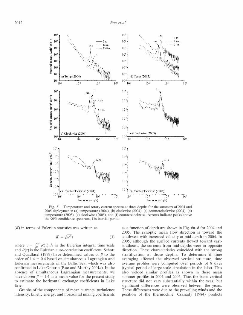
Auto and rotary spectra have been calculated for alldepths in both years. Spectra were computed using the fastFourier transform method. All spectra were computedfrom multiple, overlapping, unfiltered data subsets of 128hourly values, which were first transformed and thenensemble averaged and smoothed by Hanning filter.Furthermore, to determine if the peaks in the spectra aresignificant against a background spectrum, a red noisespectrum of univariate lag-1 autoregressive process wasutilized (Percival and Walden 1993). The 90% confidencelevels were obtained by multiplying the backgroundspectrum by the 90 percentile value of x 2

2-distribution.Figure 5a–c shows typical energy spectral density plots oftemperature and rotary spectra of currents at selecteddepths in 2004. The spectral peak of temperature (Fig. 5a)is around 24 h and corresponds to diurnal variation. Thesecondary peak appears to be close to the inertial period(18 h , 0.055 cph) and dominant in the sub-surface levels.The effects of the seasonal warming can be seen in the lowfrequency band (time scales longer than 1 day). The rotaryspectra of currents (Fig. 5b,c) show several peaks. Theclockwise spectrum of surface currents shows two signifi-cant peaks, one at 24 h and a secondary peak at 14.2 h(0.07 cph). The peak at 14.2 h appears to be the dominantpeak in the counterclockwise spectrum also. Saylor andMiller (1987) found a similar peak in their analysis andattributed it to the fundamental longitudinal seiche of thelake. The clockwise spectra of surface currents also show apeak close to 9.6 h (0.104 cph), indicating the presence ofsecondary longitudinal mode at this site. The sub-surfacecurrents are dominated by inertial oscillations, which areclearly evident in the clockwise spectrum. The inertial peak,around 18 h, is inherent to all sub-surface depths, and thispeak decreases in the hypolimnion. The mixed layer ispredominantly driven by wind and inertial forces, whereasthe hypolimnion derives its energy from large-scale windforcing. In 2005 the dominant peak is due to inertialoscillations at 15-m depth (Fig. 5d). Although the spectral

energy levels were slightly higher in 2005 than in 2004,similar characteristics were obtained (Fig. 5e,f). The energyfalls quite rapidly in the high frequency band (0.1–0.5 cph).Rao and Murthy (2001a) noted that these fluctuations arenot entirely random in this band but they contribute todispersal processes; hence, they are included in fluctuatingturbulent currents. Boyce and Chiocchio (1987) also notedthat the currents in this range are due to large-scaleturbulence. However, they did not quantify the horizontalturbulence in their study. Consequently, we use a low-passfilter with a cut-off periodicity of 8–10 h to filter out allhigh-frequency oscillations from the mean flow.

Horizontal mixing

In large lakes horizontal mixing is a consequence of bothfluctuations of the velocity field and the shear in theadvective fields. Most experimental investigations onhorizontal mixing were made with artificial tracers ordrifters (Murthy 1976; Peeters et al. 1996). On the otherhand, long time series of horizontal current fluctuations atfixed points obtained from moored current meters can alsobe interpreted in terms of mixing parameters (Lemmin1989; Rao and Murthy 2001a). Royer et al. (1987) alsoobserved that small scale fluctuations contribute tohorizontal variability of temperature in the central basin.In order to estimate horizontal exchange coefficients in themid-central basin of Lake Erie, we use current velocity dataobtained from both ADCP and Sontek Hydra stations. Ananalysis of the entire temperature and current time series ineach year will reveal an average flow regime for theduration of the whole record in response to the associatedsynoptic wind forcing. The time series of low frequency(filtered, .8 h) flow values in the previous section u(t) andv(t) are subtracted from the observed hourly values u(t)and v(t) to obtain the fluctuations u9(t) and v9(t). Thevariance (u02 and v02) is used as a measure of the magnitudeof velocity fluctuations. Here, the overbar in the variancerepresents time averaging from day 211 to day 280 for latesummer conditions.

The intensity of horizontal turbulence is calculated as theratios

iu, iv½ �~

ffiffiffiffiffiffiffiffiffiffiu0ð Þ2

qffiffiffiffiffiffiffiffiffiffiffiffiffiffiffiffiffiffiffiffiffiffiffiffi�uuð Þ2 z �vvð Þ2

q ,

ffiffiffiffiffiffiffiffiffiv0ð Þ2

qffiffiffiffiffiffiffiffiffiffiffiffiffiffiffiffiffiffiffiffiffiffiffiffi�uuð Þ2 z �vvð Þ2

q264

375 ð1Þ

which measure the magnitude of turbulent pulsationsrelative to the mean flow velocity.

The mean flow kinetic energy (MKE), and thefluctuating (turbulent) currents kinetic energy (TKE) arethen simply given as

MKE, TKEf g~1

2�uu2 z �vv2

,1

2u02 z v02 � �

ð2Þ

Rao and Murthy (2001a) developed a relationship usingTaylor’s (1921) analysis between the horizontal exchangecoefficient and the Eulerian current fluctuations in LakeOntario. In their study, the horizontal exchange coefficient

Lake Erie central basin hypoxia 2011

(K) in terms of Eulerian statistics was written as

K ~ bu02t ð3Þ

where t ~Ð?

0R tð Þ dt is the Eulerian integral time scale

and R(t) is the Eulerian auto-correlation coefficient. Schottand Quadfasel (1979) have determined values of b to theorder of 1.4 6 0.4 based on simultaneous Lagrangian andEulerian measurements in the Baltic Sea, which was alsoconfirmed in Lake Ontario (Rao and Murthy 2001a). In theabsence of simultaneous Lagrangian measurements, wehave chosen b 5 1.4 as a mean value for the present studyto estimate the horizontal exchange coefficients in LakeErie.

Graphs of the components of mean currents, turbulenceintensity, kinetic energy, and horizontal mixing coefficients

as a function of depth are shown in Fig. 6a–d for 2004 and2005. The synoptic mean flow direction is toward thesouthwest with increased velocity at mid-depth in 2004. In2005, although the surface currents flowed toward east-southeast, the currents from mid-depths were in oppositedirection. These characteristics coincided with the strongstratification at those depths. To determine if timeaveraging affected the observed vertical structure, timeaverage profiles were computed over periods of 8 days(typical period of large-scale circulation in the lake). Thisalso yielded similar profiles as shown in these meansummer profiles in 2004 and 2005. Thus the basic verticalstructure did not vary substantially within the year, butsignificant differences were observed between the years.These differences were due to the prevailing winds and theposition of the thermocline. Csanady (1984) predicts

Fig. 5. Temperature and rotary current spectra at three depths for the summers of 2004 and2005 deployments: (a) temperature (2004), (b) clockwise (2004), (c) counterclockwise (2004), (d)temperature (2005), (e) clockwise (2005), and (f) counterclockwise. Arrows indicate peaks abovethe 90% confidence spectrum, f is inertial period.

2012 Rao et al.

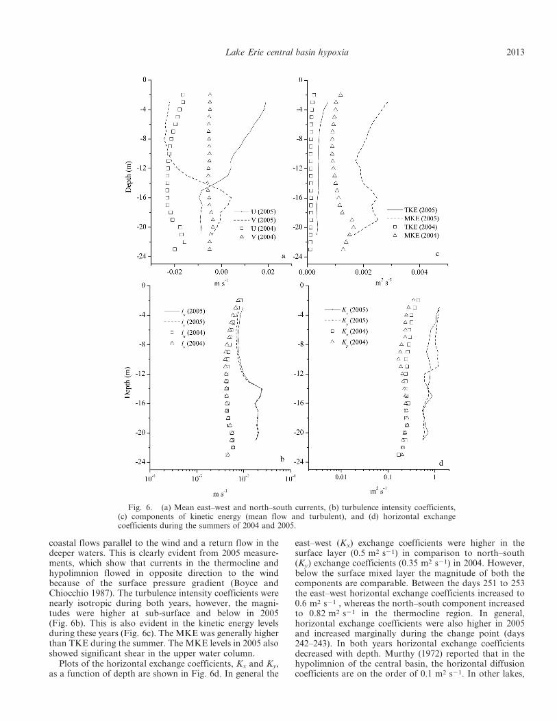
coastal flows parallel to the wind and a return flow in thedeeper waters. This is clearly evident from 2005 measure-ments, which show that currents in the thermocline andhypolimnion flowed in opposite direction to the windbecause of the surface pressure gradient (Boyce andChiocchio 1987). The turbulence intensity coefficients werenearly isotropic during both years, however, the magni-tudes were higher at sub-surface and below in 2005(Fig. 6b). This is also evident in the kinetic energy levelsduring these years (Fig. 6c). The MKE was generally higherthan TKE during the summer. The MKE levels in 2005 alsoshowed significant shear in the upper water column.

Plots of the horizontal exchange coefficients, Kx and Ky,as a function of depth are shown in Fig. 6d. In general the

east–west (Kx) exchange coefficients were higher in thesurface layer (0.5 m2 s21) in comparison to north–south(Ky) exchange coefficients (0.35 m2 s21) in 2004. However,below the surface mixed layer the magnitude of both thecomponents are comparable. Between the days 251 to 253the east–west horizontal exchange coefficients increased to0.6 m2 s21 , whereas the north–south component increasedto 0.82 m2 s21 in the thermocline region. In general,horizontal exchange coefficients were also higher in 2005and increased marginally during the change point (days242–243). In both years horizontal exchange coefficientsdecreased with depth. Murthy (1972) reported that in thehypolimnion of the central basin, the horizontal diffusioncoefficients are on the order of 0.1 m2 s21. In other lakes,

Fig. 6. (a) Mean east–west and north–south currents, (b) turbulence intensity coefficients,(c) components of kinetic energy (mean flow and turbulent), and (d) horizontal exchangecoefficients during the summers of 2004 and 2005.

Lake Erie central basin hypoxia 2013

for example in Swiss lakes, Peeters et al. (1996) obtainedhorizontal diffusivities in the range of 0.2 m2 s21 to0.3 m2 s21. Rao and Murthy (2001b) also showed thathorizontal exchange coefficients in the coastal waters ofLake Ontario varied between 0.02 m2 s21 to 2.0 m2 s21

during summer. The general range of horizontal exchangecoefficients (0.2–1.2 m2 s21) obtained in this study is,therefore, comparable to these observations.

Vertical mixing

Several mechanisms such as current shear, breaking ofinternal waves, or convective overturns contribute to thegeneration of vertical turbulence in lakes. The stronginfluence that the vertical shear and stability have onturbulence can be estimated from the gradient Richardsonnumber, Ri 5 N2/S2. Here, N is the Brunt-Vaisalafrequency given as N2 ~ { g=r0ð Þ Lr=Lzð Þ and the verticalcurrent shear S2 ~ Lu=Lzð Þ2 z Lv=Lzð Þ2, where z is thevertical coordinate positive upward; u and v are hourlyeast–west and north–south currents, respectively; g is theacceleration due to gravity, and r0 is reference density. Thedensity of the lake water was estimated from thetemperature data from thermistor moorings and calculatedaccording to Chen and Millero (1986) formula. Thetemperature data at different levels were smoothly inter-polated using a cubic spline technique to match with ADCPcurrent measurement levels.

The turbulent mixing can be calculated on the basis ofdifferent models using advanced turbulence closureschemes. However, in this study following Rao and Murthy(2001b), we employ a simple empirical formula suggestedby Pacanowski and Philander (1981). They related the eddydiffusivity (Kz) to the Richardson number and studied themodeling of temperature structure in the tropical ocean,which is given as

Kz ~Ko

1 z 5Rið Þ2z Kb ð4Þ

where Ko is an adjustable parameter and Kb is thebackground eddy diffusivity. In the present study followingOmstedt and Murthy (1994), we assign Ko 5 1022 m2 s21

and Kb 5 1027 m2 s21 to account for low eddy diffusivityvalues in the Great Lakes. Similar parameterization ofvertical mixing in terms of Richardson number has beenused in several studies (Rao et al. 2004; Loewen et al. 2007).The eddy diffusivity coefficients calculated by Eq. 4 are notquite complete, as Kz becomes constant under homoge-neous conditions. Given the uncertainties, the Kz valuesobtained here should be considered only as an order ofmagnitude estimates.

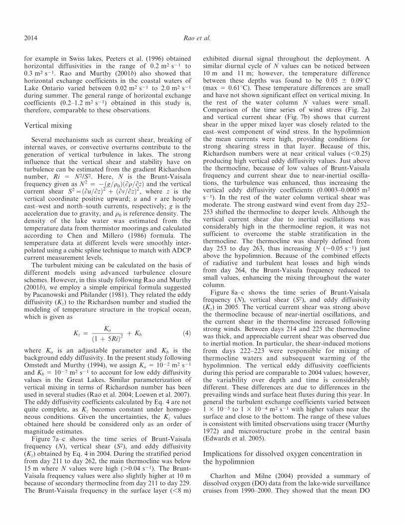
Figure 7a–c shows the time series of Brunt-Vaisalafrequency (N), vertical shear (S2), and eddy diffusivity(Kz) obtained by Eq. 4 in 2004. During the stratified periodfrom day 211 to day 262, the main thermocline was below15 m where N values were high (.0.04 s21). The Brunt-Vaisala frequency values were also slightly higher at 10 mbecause of secondary thermocline from day 211 to day 229.The Brunt-Vaisala frequency in the surface layer (,8 m)

exhibited diurnal signal throughout the deployment. Asimilar diurnal cycle of N values can be noticed between10 m and 11 m; however, the temperature differencebetween these depths was found to be 0.05 6 0.09uC(max 5 0.61uC). These temperature differences are smalland have not shown significant effect on vertical mixing. Inthe rest of the water column N values were small.Comparison of the time series of wind stress (Fig. 2a)and vertical current shear (Fig. 7b) shows that currentshear in the upper mixed layer was closely related to theeast–west component of wind stress. In the hypolimnionthe mean currents were high, providing conditions forstrong shearing stress in that layer. Because of this,Richardson numbers were at near critical values (,0.25)producing high vertical eddy diffusivity values. Just abovethe thermocline, because of low values of Brunt-Vaisalafrequency and current shear due to near-inertial oscilla-tions, the turbulence was enhanced, thus increasing thevertical eddy diffusivity coefficients (0.0003–0.0005 m2

s21). In the rest of the water column vertical shear wasmoderate. The strong eastward wind event from day 252–253 shifted the thermocline to deeper levels. Although thevertical current shear due to inertial oscillations wasconsiderably high in the thermocline region, it was notsufficient to overcome the stable stratification in thethermocline. The thermocline was sharply defined fromday 253 to day 263, thus increasing N (,0.05 s21) justabove the hypolimnion. Because of the combined effectsof radiative and turbulent heat losses and high windsfrom day 264, the Brunt-Vaisala frequency reduced tosmall values, enhancing the mixing throughout the watercolumn.

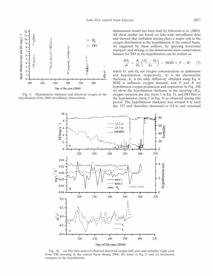
Figure 8a–c shows the time series of Brunt-Vaisalafrequency (N), vertical shear (S2), and eddy diffusivity(Kz) in 2005. The vertical current shear was strong abovethe thermocline because of near-inertial oscillations, andthe current shear in the thermocline increased followingstrong winds. Between days 214 and 225 the thermoclinewas thick, and appreciable current shear was observed dueto inertial motion. In particular, the shear-induced motionsfrom days 222–223 were responsible for mixing ofthermocline waters and subsequent warming of thehypolimnion. The vertical eddy diffusivity coefficientsduring this period are comparable to 2004 values; however,the variability over depth and time is considerablydifferent. These differences are due to differences in theprevailing winds and surface heat fluxes during this year. Ingeneral the turbulent exchange coefficients varied between1 3 1025 to 1 3 1024 m2 s21 with higher values near thesurface and close to the bottom. The range of these valuesis consistent with limited observations using tracer (Murthy1972) and microstructure probe in the central basin(Edwards et al. 2005).

Implications for dissolved oxygen concentration inthe hypolimnion

Charlton and Milne (2004) provided a summary ofdissolved oxygen (DO) data from the lake-wide surveillancecruises from 1990–2000. They showed that the mean DO

2014 Rao et al.

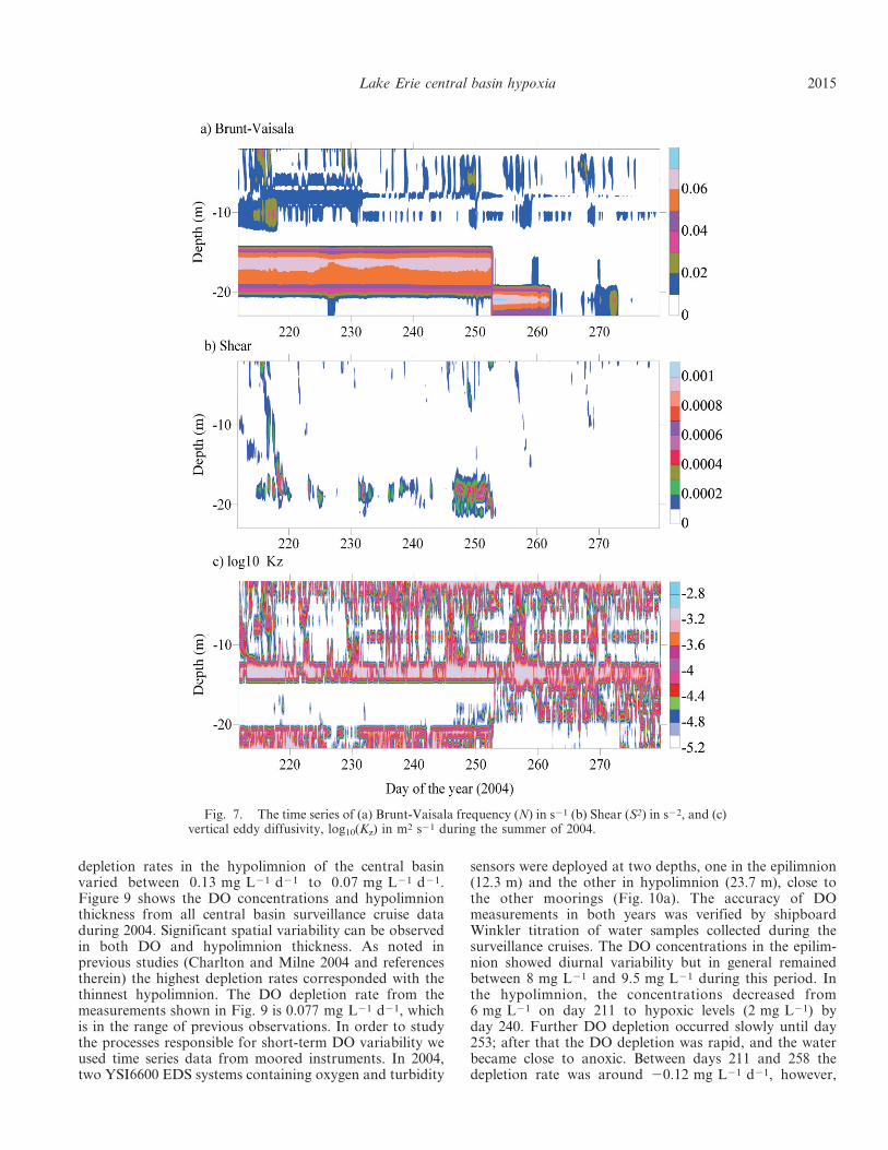
depletion rates in the hypolimnion of the central basinvaried between 0.13 mg L21 d21 to 0.07 mg L21 d21.Figure 9 shows the DO concentrations and hypolimnionthickness from all central basin surveillance cruise dataduring 2004. Significant spatial variability can be observedin both DO and hypolimnion thickness. As noted inprevious studies (Charlton and Milne 2004 and referencestherein) the highest depletion rates corresponded with thethinnest hypolimnion. The DO depletion rate from themeasurements shown in Fig. 9 is 0.077 mg L21 d21, whichis in the range of previous observations. In order to studythe processes responsible for short-term DO variability weused time series data from moored instruments. In 2004,two YSI6600 EDS systems containing oxygen and turbidity

sensors were deployed at two depths, one in the epilimnion(12.3 m) and the other in hypolimnion (23.7 m), close tothe other moorings (Fig. 10a). The accuracy of DOmeasurements in both years was verified by shipboardWinkler titration of water samples collected during thesurveillance cruises. The DO concentrations in the epilim-nion showed diurnal variability but in general remainedbetween 8 mg L21 and 9.5 mg L21 during this period. Inthe hypolimnion, the concentrations decreased from6 mg L21 on day 211 to hypoxic levels (2 mg L21) byday 240. Further DO depletion occurred slowly until day253; after that the DO depletion was rapid, and the waterbecame close to anoxic. Between days 211 and 258 thedepletion rate was around 20.12 mg L21 d21, however,

Fig. 7. The time series of (a) Brunt-Vaisala frequency (N) in s21 (b) Shear (S2) in s22, and (c)vertical eddy diffusivity, log10(Kz) in m2 s21 during the summer of 2004.

Lake Erie central basin hypoxia 2015

significant short-term changes between +0.87 mg L21 d21

and 21.16 mg L21 d21 were observed.The seasonal depletion of DO in the hypolimnion is

caused by the combination of the sediment oxygen demand(SOD) and water column oxygen demand. Values of SODmeasured by Snodgrass (1987) and Charlton (1980) in thecentral basin ranged from 0.07 mg L21 d21 to 0.035 mgL21 d21 for a 4-m-thick hypolimnion. More recently,Matisoff and Neeson (2005) estimated that SOD rate in thecentral basin was 0.080 6 20.026 mg L21 d21 in a 3–5-m-thick hypolimnion. The SOD probably explains the steadydecrease of DO concentrations on a seasonal scale, but itcannot account for the rapid variability of DO at thislocation.

While the shallow depth of the hypolimnion is animportant factor for DO budget, several other factorsinfluence the change of DO concentration in the watercolumn. The physical processes presented earlier willstrongly influence the DO concentrations in the hypolimni-on. Royer et al. (1987) showed that physical and transportprocesses produce significant changes of hypolimnioncharacteristics at short time scales (hours to days). Thesefactors are crucial for delaying the setting of anoxia in thecentral basin. Ivey and Patterson (1982) and Patterson et al.(1985) developed a one-dimensional oxygen budget modelfor the central basin of Lake Erie. Lam and Schertzer (1987)also used a similar approach for studying the relationship ofanoxic conditions in Lake Erie. More recently, a similar one-

Fig. 8. The same as Fig. 7 except for the summer of 2005.

2016 Rao et al.

dimensional model has been used by Edwards et al. (2005).All these studies are based on lake-wide surveillance dataand showed that turbulent mixing plays a major role in theoxygen distribution in the hypolimnion of the central basin.As suggested by these authors, by ignoring horizontaltransport and mixing, a one-dimensional mass conservationbalance for DO in the hypolimnion can be written as

dOh

dt~

Kz

Hd

Oe { Oh

Dz

� �{ SOD z P { Rð Þ ð5Þ

where Oe and Oh are oxygen concentrations in epilimnionand hypolimnion, respectively, Dz is the thermoclinethickness, Kz is the eddy diffusivity obtained using Eq. 4,SOD is sediment oxygen demand, and P and R arehypolimnion oxygen production and respiration. In Fig. 10bwe show the hypolimnion thickness at the mooring (Hd),oxygen variation per day (term 1 in Eq. 5), and DO flux tothe hypolimnion (term 2 in Eq. 5) as observed during thisperiod. The hypolimnion thickness was around 4 m untilday 252 and thereafter decreased to 0.8 m and remained

Fig. 10. (a) The time series of observed dissolved oxygen (left axis) and turbidity (right axis)from YSI mooring in the central basin during 2004; (b) terms in Eq. 5; and (c) horizontaltransport in the hypolimnion.

Fig. 9. Hypolimnion thickness and dissolved oxygen in thehypolimnion from 2004 surveillance observations.

Lake Erie central basin hypoxia 2017

there until the lake overturned. The small changes in thehypolimnion thickness coincided with wind-induced verticalmixing. The DO depletion varied quite rapidly within thisperiod. The DO flux due to turbulent mixing appears tobalance observed oxygen variability only on certain epi-sodes. For example, the increased turbulence due toclockwise rotating winds on day 219 contributed onlymarginally to the increased oxygen at this location. Theturbulent mixing balances the oxygen variation on day 235and played a major role during the strong wind event on day252. As suggested in previous studies these results alsoindicate that the variability of oxygen concentrations in thehypolimnion on occasions is due to the downward mixing ofoxygen. In general the hypolimnion depth alone, which wasalready thin (,4 m), did not show a significant effect on theshort-term variability of DO until day 252. Lam andSchertzer (1987) suggested that anoxia develops when thehypolimnion layer is ,4 m and vertical diffusion is low (1 31024 m2 s21). Although the turbulent diffusivity below thethermocline was low (,1 3 1024 m2 s21) from day 211 today 252, this did not result in immediate anoxic conditions.Shortly after day 253 the hypolimnion thickness dropped to0.8 m, and strong stable stratification (N . 0.05 s21) wasobserved in the thermocline. Although this had considerableeffect on oxygen depletion and the hypolimnion layer at thislocation, significant resuspension of bottom sedimentswould have also played a major role in the rapid decreasein oxygen concentrations on day 253. The bottom sedimentsin the central basin generally have a higher percentage ofeasily oxidizable substances that consume oxygen whenexposed (Davis et al. 1987). Such resuspension of bottomsediments can be clearly seen in the turbidity peak caused bythe strong easterly wind episode at this location (Fig. 10a).Bottom stresses on this day (calculated from the current andwave parameters using the method of Li and Amos 2002)exceeded 0.3 Pa, well above the stress needed to initiatebottom resuspension at this site (Lick et al. 1994). Asmentioned before, SOD (term 3 in Eq. 1) is responsible forthe gradual decrease of DO concentrations in the hypolim-nion, but it cannot account for the rapid variability of DOconcentrations.

The significant DO variability observed from day 211 to225 could also be due to the horizontal flux of oxygenbecause of horizontal mixing and transport past themooring. The mean horizontal exchange coefficients inthe hypolimnion were about 2 3 1021 m2 s21. The typicaloxygen concentration gradient in the central basin from thesurveillance cruises was 5 3 1025 mg L21 m21. This willcause a diffusive flux in the order of 1022 mg m22 s21 atthis location. Therefore it is evident that vertical mixingand the horizontal mixing together are not sufficient tobalance the observed short-term oxygen variation at thisstation. In order to verify if horizontal transport played asignificant role in the observed DO variability, we haveapproximated the mean transport in the hypolimnion as

qu ~

ðHd

0

u dz, qv ~

ðHd

0

v dz ð6Þ

Figure 10c shows the east–west (qu) and north–south (qv)

components of transport in the hypolimnion during thisperiod. It is clear that the sudden increase in oxygen levelson day 219 was due to the northwest transport of waterfrom shallow layers. The vertical velocities during thisepisode were small and positive, therefore, entrainment ofthermocline waters into the hypolimnion is not significant.The significant drop in oxygen levels on day 224 alsocoincided with the transport from the surrounding lessoxygenated waters. Figure 11 shows observations of DOconcentrations and physical processes during the 2005deployment period. During this period DO concentrationsin the epilimnion were only available from the ship-boardprofiler, whereas DO concentrations in the hypolimnionwere measured by a YSI 6600 EDS sonde at 23 m. It wasevident from 2004 measurements that DO concentrationsdo not vary significantly in the epilimnion; therefore, weuse a linear interpolation to fill the missing data in thatlayer. In general, variability of DO concentrations and itsrelation to physical processes are similar to 2004 observa-tions. These results support the view that in the hypolim-nion the heat and DO variability are affected by thehorizontal transport (Royer et al. 1987).

Discussion

The Eulerian data during the summers of 2004 and 2005in the central basin of Lake Erie show significant variabilityof currents and temperature because of differences in theforcing conditions between the years. The mean currentsthroughout the water column were directed toward thesouthwest in 2004, whereas they showed a two-layerstructure in 2005. As reported in previous studies, ourresults also suggest that the near-surface currents are wind-driven, whereas the hypolimnion motions are mainlybecause of surface pressure gradient due to wind setup.In both years the current and temperature spectra showed aprominent peak at around 18 h, indicating the presence ofclock-wise rotating inertial waves. Although the peakenergy at the high-frequency end was located mainly atthe near-inertial frequency band, significant energy wasobserved at much smaller scales, indicating the presence oflongitudinal seiche motions.

The horizontal exchange characteristics of the watercolumn are parameterized with two horizontal exchangecoefficients for momentum (Kx and Ky). The turbulenceintensity coefficients indicate near-isotropy of horizontalturbulence in the hypolimnion during both 2004 and 2005.The MKE was generally higher than TKE during thesummer. The east–west horizontal exchange coefficientswere marginally higher (0.5 m2 s21) than north–southexchange coefficients (0.35 m2 s21) in the epilimnion.

Detailed observations of currents and temperaturesduring these years are used to study the relationshipbetween vertical current shear and stratification. This studyhas demonstrated that the processes controlling the verticalmixing vary both between and within different water layers.In general the largest shear was observed above orsometimes in the thermocline and close to the bottom. Itsmagnitude varied with time following changes in wind-stress characteristics. Inertial shear dominated after strong

2018 Rao et al.

winds when the thermocline was thick in 2004 and in theearly part of 2005; however, when the thermocline was thinthe high vertical current shear was noticed in the surfacelayer. Vertical exchange coefficients (Kz) were obtained bycalculating Richardson numbers in the water column. Thegeneral range of Kz varied from 1 3 1025 to 1 31024 m2 s21. The high values are usually noticed in thesurface layer associated with strong shear and weakstratification. In both years the high values are alsoobserved just above the thermocline and near the bottomdue to enhanced vertical shear and reduced Brunt-Vaisalafrequencies. The range of Kz values during the late summerconditions were comparable to the typical values obtainedby Murthy (1972) and more recently by Edwards et al.(2005) in Lake Erie.

Although eutrophication is a contributor to hypolim-netic hypoxia, physical factors play a major role indissolved oxygen budget (Charlton 1980). The lake-widesurveillance data show strong spatial variability of bothhypolimnion thickness and dissolved oxygen concentra-tions in the central basin. In general, the hypolimnionthickness decreased during the summer coinciding with

decreasing DO concentrations in the hypolimnion. Iveyand Boyce (1982) suggested that the changes in hypolim-netic thickness were due to entrainment of thermoclinewaters into the hypolimnion caused by shearing stresses atthe bottom. The vertical velocity measurements from theADCPs provided limited support for such vertical trans-port mechanism in 2004 and 2005, whereas previouslyneglected wave-induced orbital motions appear to play asignificant role in generation of shearing stresses duringenergetic wind events. The time series measurements of DOin the epilimnion and hypolimnion highlight the signifi-cance of physical processes in the short-term variability ofDO in the hypolimnion. Although the mean depletion ratewas around 20.12 mg L21 d21 between days 211 and 258,significant short-term changes between +0.87 and21.16 mg L21 d21 were observed. The effect of hypolim-nion thickness of 4 m was not significant on the short-termvariability of DO in 2004. In certain strong wind conditionsvertical mixing played a significant role in balancing theoxygen budget. The strong advective currents weresometimes responsible for sudden variations of DOconcentrations in the hypolimnion. These measurements

Fig. 11. The same as Figure 10 except for the summer of 2005.

Lake Erie central basin hypoxia 2019

also show a resuspension event on day 253 and itsimportance in decreasing the DO concentrations in thehypolimnion. The sharp and persistent thermocline (N .0.05 s21) combined with shallow hypolimnion was respon-sible for the sustained anoxia at this location. The presentstudy was based on 2-year high-resolution currents andtemperature measurements in the vertical at one location;to confirm the spatial and temporal variability of thesefindings it is necessary to conduct these intensive studies atother selected sites in the central basin. However, theseresults further confirm the importance of physical processesand the need of proper incorporation of these processes innumerical models.

References

BOYCE, F. M., M. N. CHARLTON, D. RATHKE, C. H. MORTIMER,AND J. R. BENNETT [EDS.]. 1987. Lake Erie Bi-national Study1979–1980. J. Great Lakes Res. Special Issue 13.

———, AND F. CHIOCCHIO. 1987. Water movements at a mid-central basin site: Time and space scales, relation to wind andinternal pressure gradients. J. Great Lakes Res. 13: 530–541.

———, ——— , B. EID, F. PENICKA, AND F. ROSA. 1980.Hypolimnion flow between the central and eastern basins ofLake Erie during 1977 (Interbasin Hypolimnion Flows). J.Great Lakes Res. 6: 290–306.

BURNS, N. M., AND C. ROSS. 1972. Project Hypo, Paper No. 6,Canada Centre for Inland Waters, Burlington, Ontario.USEPA Tech. Report TS-05-71-208-24.

CHARLTON, M. N. 1980. Oxygen depletion in Lake Erie: Has therebeen any change? Can. J. Fish. Aquat. Sci. 37: 72–81.

———, AND J. MILNE. 2004. Review of thirty years of change inLake Erie water quality, NWRI Contribution No. 04-167.National Water Research Institute.

CHEN, C. T. A., AND F. J. MILLERO. 1986. Precise thermodynamicproperties for natural waters covering only the limnologicalrange. Limnol. Oceanogr. 31: 657–662.

CSANADY, G. T. 1984. Circulation in the coastal ocean. D. Reidel.DAVIS, W. S., L. A. FAY, AND C. E. HERDENDORF. 1987. Overview

of USEPA/CLEAR Lake Erie Sediment Oxygen demandinvestigations during 1979. J. Great Lakes Res. 13: 731–737.

EDWARDS, W. J., J. D. CONROY, AND D. A. CULVER. 2005.Hypolimnetic oxygen depletion dynamics in the central basinof Lake Erie. J. Great Lakes Res. 31: 262–271.

HAMBLIN, P. F. 1987. Meteorological forcing and water levelfluctuations on Lake Erie. J. Great Lakes Res. 13: 436–453.

HAWLEY, N., AND oTHERS. 2006. Hypoxia in Lake Erie and TheInternational Field Years for Lake Erie (IFYLE), EOS.Transactions of American Geophysical Union 87: 313–319.

IVEY, G. N., AND F. M. BOYCE. 1982. Entrainment by bottomcurrents in Lake Erie. Limnol. Oceanogr. 27: 1029–1034.

———, AND J. C. PATTERSON. 1984. A model of the vertical mixingin Lake Erie in summer. Limnol. and Oceanogr. 29: 553–563.

LAM, D. C. L., AND W. M. SCHERTZER. 1987. Lake Eriethermocline model results: Comparison with 1987–1982 dataand relation to anoxic occurrences. J. Great Lakes Res. 13:757–769.

———, ———, AND R. C. MCCRIMMON. 2002. Modelling changesin phosphorus and dissolved oxygen pre- and post-zebramussel arrival in Lake Erie, NWRI Contribution No. 02-198.National Water Research Institute.

LEMMIN, U. 1989. Dynamics of horizontal mixing in the nearshorezone of Lake Geneva. Limnol. Oceanogr. 34: 420–434.

LOEWEN, M. R., J. D. ACKERMAN, AND P. F. HAMBLIN. 2007.Environmental implications of stratification and turbulentmixing in a shallow lake basin. Can. J. Fish. Aquat. Sci. 64:43–57.

MATISOFF, G., AND T. M. NEESON. 2005. Oxygen concentrationand demand in Lake Erie sediments. J. Great Lakes Res. 31:284–295.

MURTHY, C. R. 1972. An investigation of diffusion characteristicsof the hypolimnion of Lake Erie, p. 39–44. In Project Hypo,Paper No. 6, Canada Centre for Inland Waters, Burlington,Ontario. USEPA Tech. Rept. TS-05-71-208–24.

———. 1976. Horizontal diffusion characteristics in LakeOntario. J. Phys. Oceanogr. 6: 76–84.

OMSTEDT, A., AND C. R. MURTHY. 1994. On currents and verticalmixing in lake Ontario during summer stratification. NordicHydrology 25: 213–232.

PACANOWSKI, R. C., AND S. G. PHILANDER. 1981. Parameterizationof vertical mixing in numerical models of tropical oceans. J.Phys. Oceanogr. 11: 1443–1451.

PATTERSON, J. C., B. R. ALLISON, AND G. N. IVEY. 1985. Adissolved oxygen budget model for Lake Erie in summer.Freshw. Biol. 15: 683–694.

PEETERS, F., A. WUEST, G. PIEPKE, AND D. M. IMBODEN. 1996.Horizontal mixing in lakes. J. Geophys. Res. 101: 18,361–18,375.

PERCIVAL, D. B., AND A. T. WALDEN. 1993. Spectral analysis forphysical applications. Cambridge Univ. Press.

RAO, Y. R., AND C. R. MURTHY. 2001a. Coastal boundary layercharacteristics during summer stratification in Lake Ontario.J. Phys. Oceanogr. 31: 1088–1104.

———, AND ———. 2001b. Nearshore currents and turbulentexchange characteristics during upwelling and downwellingevents in Lake Ontario. J. Geophys. Res. 106: 2667–2678.

———, M. G. SKAFEL, AND M. N. CHARLTON. 2004. Circulationand turbulent exchange characteristics during the thermal barin Lake Ontario. Limnol. Oceanogr. 49: 2190–2200.

ROYER, L., F. CHIOCCHIO, AND F. M. BOYCE. 1987. Tracking short-term physical and biological changes in the central basin ofLake Erie. J. Great Lakes Res. 13: 587–606.

SAYLOR, J. H., AND G. S. MILLER. 1987. Studies of large-scalecurrents in Lake Erie, 1979–80. J. Great Lakes Res. 13:487–514.

SCHERTZER, W. M. 1987. Heat balance and heat storage estimatesfor Lake Erie, 1967 to 1982. J. Great Lakes Res. 13: 454–467.

SCHOTT, F., AND D. QUADFASEL. 1979. Lagrangian and Eulerianmeasurements of horizontal mixing in the Baltic. Tellus. 31:138–144.

SNODGRASS, W. J. 1987. Analysis of models and measurements forsediment oxygen demand in Lake Erie. J. Great Lakes Res.13: 738–756.

TAYLOR, G. I. 1921. Diffusion by continuous movements. Proc.London Math. Soc. 20: 196–212.

VOLLENWEIDER, R. A. 1968. Scientific fundamentals of theeutrophication of lakes and flowing waters with particularreference to nitrogen and phosphorus as factors in eutrophi-cation. Organization for Economic Co-Operation and Devel-opment. DAS/CSI/68.27.

WU, J. 1980. Wind-stress coefficients over sea surface near neutralconditions—a revisit. J. Phys. Oceanogr. 10: 727–740.

Received: 2 November 2006Amended: 22 February 2008

Accepted: 2 April 2008

2020 Rao et al.