Wind Energ. Sci., 1, 115–128, 2016www.wind-energ-sci.net/1/115/2016/doi:10.5194/wes-1-115-2016© Author(s) 2016. CC Attribution 3.0 License.

Year-to-year correlation, record length, andoverconfidence in wind resource assessment

Nicola Bodini1,2, Julie K. Lundquist1,3, Dino Zardi2, and Mark Handschy4,5

1Department of Atmospheric and Oceanic Sciences, University of Colorado Boulder, Boulder, Colorado, USA2Department of Civil, Environmental and Mechanical Engineering, University of Trento, Trento, Italy

3National Renewable Energy Laboratory, Golden, Colorado, USA4Enduring Energy, LLC, Boulder, Colorado, USA

5Cooperative Institute for Research in the Environmental Sciences, University of Colorado Boulder,Boulder, Colorado, USA

Correspondence to: Mark Handschy (mark.handschy@colorado.edu)

Received: 22 April 2016 – Published in Wind Energ. Sci. Discuss.: 2 May 2016Revised: 20 July 2016 – Accepted: 12 August 2016 – Published: 24 August 2016

Abstract. Interannual variability of wind speeds presents a fundamental source of uncertainty in preconstruc-tion energy estimates. Our analysis of one of the longest and geographically most widespread extant sets ofinstrumental wind-speed observations (62-year records from 60 stations in Canada) shows that deviations frommean resource levels persist over many decades, substantially increasing uncertainty. As a result of this per-sistence, the performance of each site’s last 20 years diverges more widely than expected from the P50 levelestimated from its first 42 years: half the sites have either fewer than 5 or more than 15 years exceeding theP50 estimate. In contrast to this 10-year-wide interquartile range, a 4-year-wide range (2.5 times narrower) wasfound for “control” records where statistical independence was enforced by randomly permuting each station’shistorical values. Similarly, for sites with capacity factor of 0.35 and interannual variability of 6 %, one wouldexpect 9 years in 10 to fall in the range 0.32–0.38; we find the actual 90 % range to be 0.27–0.43, or three timeswider. The previously un-quantified effect of serial correlations favors a shift in resource-assessment thinkingfrom a climatology-focused approach to a persistence-focused approach: for this data set, no improvement inP50 error is gained by using records longer than 4–5 years, and use of records longer than 20 years actuallydegrades accuracy.

1 Introduction

Wind power is becoming less expensive and nowadays rep-resents a very attractive low-emissions choice for electricityproduction. Its economy depends on generation plants be-ing sited where enough wind blows to make developmentworthwhile; “resource assessments” are intended to iden-tify such sites. Assessments can be carried out in differentways (Landberg et al., 2003), but predictions about futurewind “climate” are based on historical observations. To pro-vide sufficient history without decades of delay while mea-surements are collected at a target site, so-called measure–correlate–predict (MCP) techniques are used to infer windresource levels by correlation with a longer record available

for a nearby reference site. A wide variety of functional re-lationships have been investigated; see reviews by Brower(2012) and by Carta et al. (2013).

Resource assessment inaccuracies and uncertainties arisenot only from less than perfect target and/or reference wind-speed correlation, including missing data (Salmon and Tay-lor, 2014), but also from many instrumental and model uncer-tainties (Mortensen et al., 2013; Lackner et al., 2008). Here,though, we focus on the “Predict” step in resource assess-ment. To avoid uncertainties associated with the full energyassessment, such as the modeling of flow over complex ter-rain, extrapolation of wind speeds to hub height, wake losses,turbine availability, and so on, we analyze only the extent to

Published by Copernicus Publications on behalf of the European Academy of Wind Energy e.V.

116 N. Bodini et al.: Overconfidence in wind resource assessment

which historical anemometer measurements can be used topredict future ranges of the same anemometer measurements.(We convert anemometer measurements to modeled turbinecapacity factor just to give an appropriate variability scale.)

Given wind’s natural variability, an important question ishow long a history is needed to both adequately estimate itsmean level and to characterize the range of expected year-to-year variation. Previous authors have been of two minds.Justus et al. (1979) and Corotis (1980) both concluded thata single year’s measurements were sufficient to give an esti-mate of the long-term mean accurate to 10 % with 90 % con-fidence, and that correlation with longer records at nearbysites offered the potential for only marginal improvement.Concern over possible trends and the magnitude of variabil-ity over longer horizons, though, has driven examination ofmulti-decadal winds, using both direct observations (Palu-tikof et al., 1985; Earl et al., 2012; Früh, 2013; Azorin etal., 2014; Watson et al., 2015), and reconstructions using nu-merical weather prediction (NWP) reanalysis data (Palutikofet al., 1992; Albers, 2004; Bett et al., 2013; Kirchner-Bossiet al., 2014; Bett et al., 2016), with the uncertainties of re-analysis data examined by Rose and Apt (2015, 2016). Con-sidering seven sites in Great Britain and Ireland, each withmore than 55 years of records, Palutikof et al. (1985) sug-gested, “it is vital to consider the longest available wind-speed records, in order to obtain the best possible estimateof the range of variability of the future wind regime”. Ana-lyzing a 125-year reconstruction of geostrophic winds (windscomputed from surface atmospheric pressure measurements)in Germany, Albers (2004) found that the error in “predict-ing” the mean of a given 20-year period decreased as thelength of the preceding period on which the estimate wasbased increased, until the length of the estimating period hadincreased to about 35 years. On this basis he recommendedthat resource assessments should be based on a historicalrecord of at least 30 years’ length. Taking a middle ground,Brower (2012, p. 163) stated “the benefit of going beyondabout 10–15 years of reference data is limited”. The effects ofcorrelation between measurements made at times more thana few hours apart are rarely considered in published anal-yses of resource-assessment methodologies, although hub-height wind speeds exhibit anomalies persisting for at least12 months (Klink, 2007) that complicate regression analysis(Pryor and Ledolter, 2010).

Here, we focus on how statistics derived from historicaltime-series records are used to predict the future exceedancelevels employed in resource assessments. We use 62 yearsof homogenized monthly wind speed records from 60 Cana-dian stations (Environment and Climate Change Canada,2016), as described in Sect. 2. To reveal the consequencesof any unwarranted assumptions of statistical independence,we analyze for each station both its actual record and a“control” record of statistically independent values producedby randomly permuting the station’s chronological values.We quantify estimation inaccuracy both as exceedance er-

rors and as energy errors, using concepts also introducedin Sect. 2. As we describe in Sect. 3, comparing the errorsin estimates made from the chronological and randomizedrecords unambiguously reveals that interannual correlationsare responsible for larger than expected estimation errors andalso for the growth of these errors with record length. Thisresult is consistent with a slow power-law decay of year-to-year correlation, or “long-term persistence”, which we dis-cuss further in Sect. 4, and suggest that estimators explicitlyaccounting for year-to-year correlation behavior would en-able both more accurate predictions and a correct assessmentof confidence.

2 Data and methods

2.1 Canadian wind speed data set

We base our analysis here on one of the longer observationaldata sets of instrumental wind speed records available, a 62-year (1953–2014) record of monthly average wind speedsfrom 156 Canadian meteorological stations (Environmentand Climate Change Canada, 2016). The stations stretch east-to-west from Vancouver to Halifax and north-to-south fromthe U.S. border to the Arctic Circle. These data, from the Na-tional Climate Data Archive of Environment Canada, havebeen carefully homogenized by Wan et al. (2010). The ho-mogenization process adjusted all wind speeds recorded atnonstandard anemometer heights to 10 m height using a log-arithmic profile and surface-roughness-length data. Further,mean shifts from changes in anemometer height, type, or lo-cation, whether recorded in station histories or detected bystatistical testing as part of the homogenization process, werealso adjusted by comparison of each station’s observationalwind-speed record with a geostrophic wind reconstructionfrom independent surface pressure data. Using the homog-enized data, Wan et al. (2010) found statistically significantdownward trends in wind speed over the period over mostof Canada except the Arctic and Maritime provinces, whichexhibited an upward trend. St. Martin et al. (2015) used a re-lated wind speed data set to investigate spatial correlation andgeographic diversity in the wind resource.

2.2 From wind speed to capacity factors

For more relevance to wind-turbine energy production weconvert monthly Environment Canada wind speeds to mod-eled turbine capacity factor (monthly electric energy pro-duction divided by turbine capacity). Since we begin withmonthly averages the conversion is necessarily crude; withour interests focused on correlation effects, though, it suf-fices that low wind speeds translate to low capacity factor andhigh wind speeds to high capacity factor, with a variabilityscale comparable to that of real wind plant. Since we judgeresource-assessment accuracy by comparing the exceedancelevels in the final 20 years of each site’s data to estimates

Wind Energ. Sci., 1, 115–128, 2016 www.wind-energ-sci.net/1/115/2016/

N. Bodini et al.: Overconfidence in wind resource assessment 117

based on the previous years’ data, systematic conversion er-rors will not affect accuracy so long as we treat data from thefinal 20 years and from the preceding years in the same way.

As shown by Lackner et al. (2008), the errors introducedby deriving capacity factors from a Weibull or Rayleighstatistical model of wind-speed distribution instead of di-rectly from a wind-speed time series are only a few per-cent. We suppose that a monthly mean value u in the En-vironment Canada records arises as the average of more-frequently-sampled wind speed values u′ drawn from aWeibull distribution having cumulative distribution function1− exp[−(u′/c)k] with shape factor k = 2 and scale factorc = 2π−1/2u; we convert speeds u′ drawn from this distri-bution into instantaneous capacity factors x′ using a powercurve loosely modeled on that of a 1.5-MW-class turbine:

x′ =v1+ b · v1

3

[v0β + (v1+ b · v13)β ]1/β, (1)

where v1 ≡ (au′−3.5ms−1)/(13.5−3.5ms−1) is a normal-ized instantaneous hub-height wind speed, and parametersv0 = 2.244, b = 3.72, and β = 5.21 control the power-curveshape. For all but the two windiest stations we set a = 1.35=(80/10)(1/7), to account for wind speeds being greater at 80 mhub height than at 10 m measurement height according to awind-profile power law with exponent appropriate for neutralstability conditions (Walter et al., 2009). For those two sta-tions, with 10 m average wind speeds of 7.6 and 8.3 m s−1,we set a = 1 to avoid having sustained operation at ratedpower compress the modeled capacity-factor variability scale(or equivalently, “to model a larger turbine”). We set x′ tozero for au′ < 3.5 m s−1. We do not model turbine cut-out asthis complication has a negligible effect on variability scale.Averaging the x′ values for a given u by Monte Carlo simula-tion yields the corresponding monthly mean capacity factorx(u), which we parameterize as

x(u)= 1.08v2

2.5

1+ v23.27 , (2)

for au≥ 0.922 m s−1 (otherwise, 0) using a second normal-ized wind speed v2 ≡ (au− 0.922ms−1)/(8.835ms−1).

To avoid any effects of seasonal cycles in the subsequentanalysis, we average the 12 monthly capacity factor valuesin a calendar year, and then work with these annual averages,62 per station. To deal with data gaps, unavoidably present insuch an extended data set, we assign null weights to missingmonthly data. Furthermore, for each station we calculate anaverage seasonal cycle as the average of all the Januaries, allthe Februaries, and so on (for both wind speed and modeledcapacity factor) over the station’s 62-year record. In yearswhere our annual average is calculated from less than 12 datapoints, we then make an adjustment according to the fractionthe available data represent of the average seasonal cycle. Allthe statistical functions calculated in the following analysisare thus weighted to take into account how many data pointsare available.

60 selected stationsLow capacity factor stationsPoor data- quality stations

0.0

0.1

0.2

0.3

0.4

0.5

0.6

0.7

σ/μ

0.0 0.1 0.2 0.3 0.4 0.5

62-year average capacity factor μ

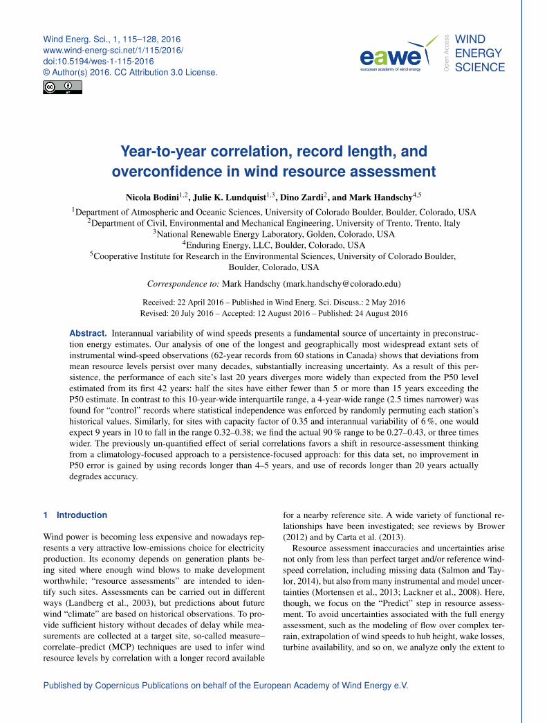
Figure 1. Ratio of the standard deviation σ of the 62 annual averagecapacity factors to their mean µ, vs. µ, for each station. Filled sym-bols: the 60 selected stations; open symbols: the discarded stations.Dashed line is the least-squares linear trend for all the 156 stations(slope of −0.47, R2

= 0.39); solid line is the least-squares lineartrend for the 60 selected stations (slope of −0.24, R2

= 0.15).

2.3 Stations selection process

In line with our focus on energy resource assessment, weeliminated from further consideration those stations withwind speeds too low for practical wind turbine deployment.We calculated, for each station, the ratio of the (weighted,always according to the number of available data) standarddeviation σ of the 62 annual average capacity factors to their62-year weighted average µ. This simple indicator of vari-ability is plotted vs.µ in Fig. 1. The least-squares linear trendin the plot reveals that the less windy sites tend to be morevariable (R2

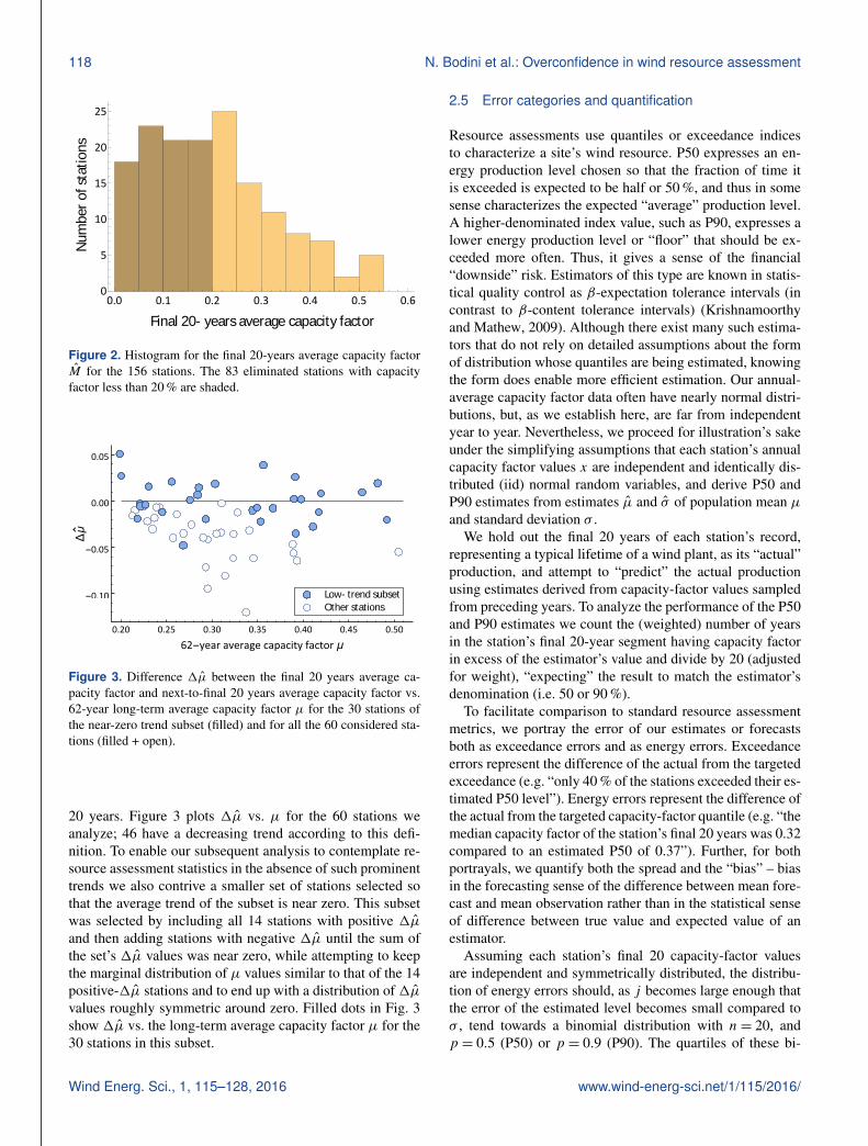
= 0.39), in accordance with the findings of Roseand Apt (2015). For each of the 156 stations, we further cal-culated the final 20-years average capacity factor M , where20 years are considered in our work as the expected lifetimeof a wind plant, yielding the distribution plotted in Fig. 2. Asthe histogram shows, there is a significant number of stationsthat, using the 1.5 MW turbine, would have low capacity fac-tors; to focus on the most plausible sites we eliminated fromfurther analysis the 83 stations with capacity factor less than20 %. Imposing this cut-off also reduced the trend observedin Fig. 1 (R2

= 0.15). We further eliminate another 13 sta-tions that have more than a single isolated year with no orscant monthly data. Nine of the remaining 60 stations hada single year with no recorded monthly values; one had 2years missing. In these cases, we fill in the missing annualvalue with the arithmetic mean of the values of the precedingand following years.

2.4 Trends and need for a 30-stations subset

Wan et al. (2010) found significant decreasing trends in windspeeds for most of the Canadian stations. We quantified thesetrends by calculating1µ, the difference between the averagecapacity factors of the final 20 years and the next-to-final

www.wind-energ-sci.net/1/115/2016/ Wind Energ. Sci., 1, 115–128, 2016

118 N. Bodini et al.: Overconfidence in wind resource assessment

0.0 0.1 0.2 0.3 0.4 0.5 0.60

5

10

15

20

25

Final 20- years average capacity factor

Num

bero

fsta

tions

Figure 2. Histogram for the final 20-years average capacity factorM for the 156 stations. The 83 eliminated stations with capacityfactor less than 20 % are shaded.

Low- trend subsetOther stations

-0.10

-0.05

0.00

0.05

Δμ

0.20 0.25 0.30 0.35 0.40 0.45 0.50

62-year average capacity factor μ

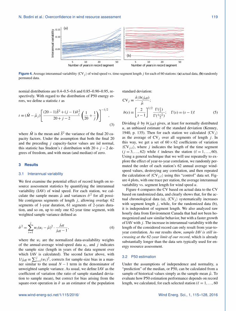
Figure 3. Difference 1µ between the final 20 years average ca-pacity factor and next-to-final 20 years average capacity factor vs.62-year long-term average capacity factor µ for the 30 stations ofthe near-zero trend subset (filled) and for all the 60 considered sta-tions (filled + open).

20 years. Figure 3 plots 1µ vs. µ for the 60 stations weanalyze; 46 have a decreasing trend according to this defi-nition. To enable our subsequent analysis to contemplate re-source assessment statistics in the absence of such prominenttrends we also contrive a smaller set of stations selected sothat the average trend of the subset is near zero. This subsetwas selected by including all 14 stations with positive 1µand then adding stations with negative 1µ until the sum ofthe set’s 1µ values was near zero, while attempting to keepthe marginal distribution of µ values similar to that of the 14positive-1µ stations and to end up with a distribution of1µvalues roughly symmetric around zero. Filled dots in Fig. 3show 1µ vs. the long-term average capacity factor µ for the30 stations in this subset.

2.5 Error categories and quantification

Resource assessments use quantiles or exceedance indicesto characterize a site’s wind resource. P50 expresses an en-ergy production level chosen so that the fraction of time itis exceeded is expected to be half or 50 %, and thus in somesense characterizes the expected “average” production level.A higher-denominated index value, such as P90, expresses alower energy production level or “floor” that should be ex-ceeded more often. Thus, it gives a sense of the financial“downside” risk. Estimators of this type are known in statis-tical quality control as β-expectation tolerance intervals (incontrast to β-content tolerance intervals) (Krishnamoorthyand Mathew, 2009). Although there exist many such estima-tors that do not rely on detailed assumptions about the formof distribution whose quantiles are being estimated, knowingthe form does enable more efficient estimation. Our annual-average capacity factor data often have nearly normal distri-butions, but, as we establish here, are far from independentyear to year. Nevertheless, we proceed for illustration’s sakeunder the simplifying assumptions that each station’s annualcapacity factor values x are independent and identically dis-tributed (iid) normal random variables, and derive P50 andP90 estimates from estimates µ and σ of population mean µand standard deviation σ .

We hold out the final 20 years of each station’s record,representing a typical lifetime of a wind plant, as its “actual”production, and attempt to “predict” the actual productionusing estimates derived from capacity-factor values sampledfrom preceding years. To analyze the performance of the P50and P90 estimates we count the (weighted) number of yearsin the station’s final 20-year segment having capacity factorin excess of the estimator’s value and divide by 20 (adjustedfor weight), “expecting” the result to match the estimator’sdenomination (i.e. 50 or 90 %).

To facilitate comparison to standard resource assessmentmetrics, we portray the error of our estimates or forecastsboth as exceedance errors and as energy errors. Exceedanceerrors represent the difference of the actual from the targetedexceedance (e.g. “only 40 % of the stations exceeded their es-timated P50 level”). Energy errors represent the difference ofthe actual from the targeted capacity-factor quantile (e.g. “themedian capacity factor of the station’s final 20 years was 0.32compared to an estimated P50 of 0.37”). Further, for bothportrayals, we quantify both the spread and the “bias” – biasin the forecasting sense of the difference between mean fore-cast and mean observation rather than in the statistical senseof difference between true value and expected value of anestimator.

Assuming each station’s final 20 capacity-factor valuesare independent and symmetrically distributed, the distribu-tion of energy errors should, as j becomes large enough thatthe error of the estimated level becomes small compared toσ , tend towards a binomial distribution with n= 20, andp = 0.5 (P50) or p = 0.9 (P90). The quartiles of these bi-

Wind Energ. Sci., 1, 115–128, 2016 www.wind-energ-sci.net/1/115/2016/

N. Bodini et al.: Overconfidence in wind resource assessment 119

(a)

0.05

0.10

0.15

Inte

rann

ualv

aria

bilit

y

105 20 50

Number of years in record segment

(b)

105 20 50

Number of years in record segment

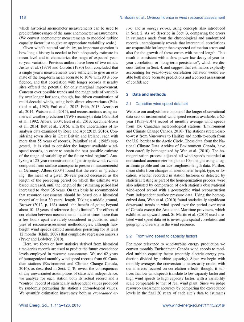
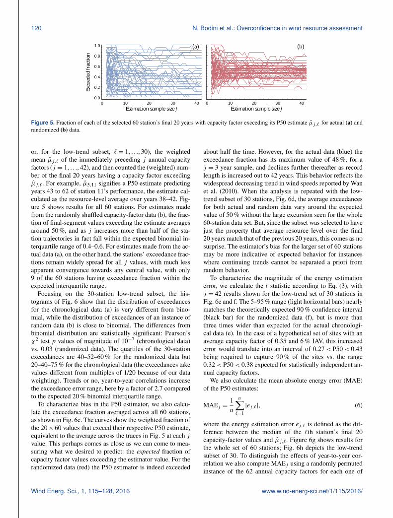
Figure 4. Average interannual variability 〈CVj 〉 of wind speed vs. time-segment length j for each of 60 stations: (a) actual data, (b) randomlypermuted data.

nomial distributions are 0.4–0.5–0.6 and 0.85–0.90–0.95, re-spectively. With regard to the distribution of P50 energy er-rors, we define a statistic t as

t ≡ (M − µj )

[(20− 1)S2

+ (j − 1)σ 2j

20+ j − 2

(120+

1j

)]−1/2

,

(3)

where M is the mean and S2 the variance of the final 20 ca-pacity factors. Under the assumption that both the final 20and the preceding j capacity-factor values are iid normal,this statistic has Student’s t distribution with 20+ j − 2 de-grees of freedom, and with mean (and median) of zero.

3 Results

3.1 Interannual variability

We first examine the potential effect of record length on re-source assessment statistics by quantifying the interannualvariability (IAV) of wind speed. For each station, we cal-culate the sample means µ and variances σ 2 for all possi-ble contiguous segments of length j , allowing overlap: 62segments of 1-year duration, 61 segments of 2-years dura-tion, and so on, up to only one 62-year time segment, withweighted sample variance defined as

σ 2=

j∑i=1

wi(ui − µ)2·jeff

jeff− 1, (4)

where the wi are the normalized data-availability weightsof the annual-average wind-speed data ui , and j indicatesthe sample size (length in years of the data segment overwhich IAV is calculated). The second factor above, with1/jeff ≡

∑j

i=1(wi)2, corrects for sample-size bias in a man-ner similar to the usual N − 1 term in the denominator ofunweighted sample variance. As usual, we define IAV as thecoefficient of variation (the ratio of sample standard devia-tion to sample mean), but correct for bias arising from thesquare-root operation in σ as an estimator of the population

standard deviation:

CVj ≡σ/b(jeff)

µ;

b(s)≡[

2s− 1

]1/2 0( s2 )

0( s−12 ); 0(s)= (s− 1)! (5)

Dividing σ by b(jeff) gives, at least for normally distributedu, an unbiased estimate of the standard deviation (Kenney,1940, p. 135). Then for each station we calculated 〈CVj 〉as the average of CVj over all segments of length j . Inthis way, we get a set of 60× 62 coefficients of variation〈CVj,`〉, where j indicates the length of the time segment(j = 3, . . .,62) while ` indexes the station (`= 1, . . .,60).Using a general technique that we will use repeatedly to ex-plore the effect of year-to-year correlation, we randomly per-muted the order of each station’s 62 annual average wind-speed values, destroying any correlation, and then repeatedthe calculation of 〈CVj,`〉 using this “control” data set. Fig-ure 4 plots, with one trace per station, the average interannualvariability vs. segment length for wind speed u.

Figure 4 compares the CV based on actual data to the CVbased on randomized data, and clearly shows that, for the ac-tual chronological data (a), 〈CVj 〉 systematically increaseswith segment length j , while, for the randomized data (b),it is independent of segment length. We also analyzed rawhourly data from Environment Canada that had not been ho-mogenized and saw similar behavior, but with a faster growthof IAV with j . The increase in interannual variability with thelength of the considered record can only result from year-to-year correlation. As our results show, sample IAV is still in-creasing at the 62-year limit of our record, which is alreadysubstantially longer than the data sets typically used for en-ergy resource assessment.

3.2 P50 estimation

Under the assumptions of independence and normality, a“prediction” of the median, or P50, can be calculated from asample of historical values simply as the sample mean µ. Toevaluate how P50 estimation performance depends on recordlength, we calculated, for each selected station (`= 1, . . .,60

www.wind-energ-sci.net/1/115/2016/ Wind Energ. Sci., 1, 115–128, 2016

120 N. Bodini et al.: Overconfidence in wind resource assessment

(a)

0.0

0.2

0.4

0.6

0.8

1.0

Exce

eded

frac

tion

0 10 20 30 40

Estimation sample size j

(b)

0 10 20 30 40

Estimation sample size j

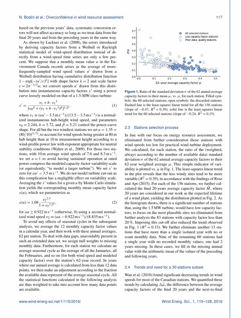
Figure 5. Fraction of each of the selected 60 station’s final 20 years with capacity factor exceeding its P50 estimate µj,` for actual (a) andrandomized (b) data.

or, for the low-trend subset, `= 1, . . .,30), the weightedmean µj,` of the immediately preceding j annual capacityfactors (j = 1, . . .,42), and then counted the (weighted) num-ber of the final 20 years having a capacity factor exceedingµj,`. For example, µ5,11 signifies a P50 estimate predictingyears 43 to 62 of station 11’s performance, the estimate cal-culated as the resource-level average over years 38–42. Fig-ure 5 shows results for all 60 stations. For estimates madefrom the randomly shuffled capacity-factor data (b), the frac-tion of final-segment values exceeding the estimate averagesaround 50 %, and as j increases more than half of the sta-tion trajectories in fact fall within the expected binomial in-terquartile range of 0.4–0.6. For estimates made from the ac-tual data (a), on the other hand, the stations’ exceedance frac-tions remain widely spread for all j values, with much lessapparent convergence towards any central value, with only9 of the 60 stations having exceedance fraction within theexpected interquartile range.

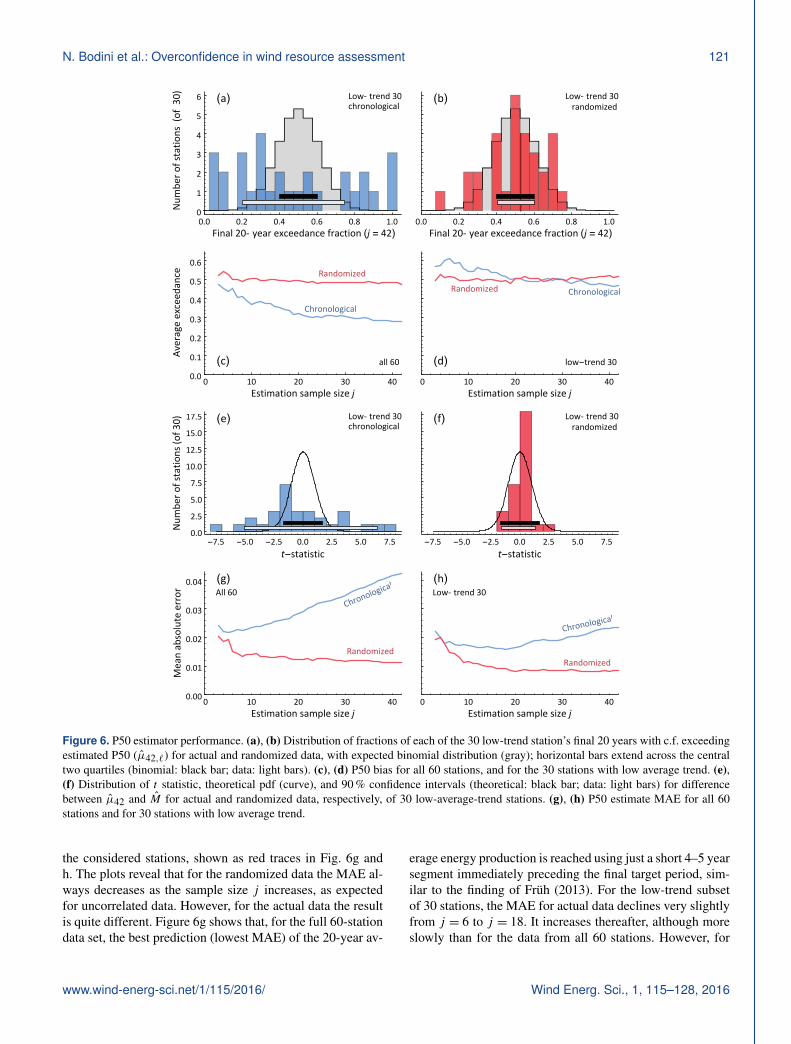
Focusing on the 30-station low-trend subset, the his-tograms of Fig. 6 show that the distribution of exceedancesfor the chronological data (a) is very different from bino-mial, while the distribution of exceedances of an instance ofrandom data (b) is close to binomial. The differences frombinomial distribution are statistically significant: Pearson’sχ2 test p values of magnitude of 10−7 (chronological data)vs. 0.03 (randomized data). The quartiles of the 30-stationexceedances are 40–52–60 % for the randomized data but20–40–75 % for the chronological data (the exceedances takevalues different from multiples of 1/20 because of our dataweighting). Trends or no, year-to-year correlations increasethe exceedance error range, here by a factor of 2.7 comparedto the expected 20 % binomial interquartile range.

To characterize bias in the P50 estimator, we also calcu-late the exceedance fraction averaged across all 60 stations,as shown in Fig. 6c. The curves show the weighted fraction ofthe 20× 60 values that exceed their respective P50 estimate,equivalent to the average across the traces in Fig. 5 at each jvalue. This perhaps comes as close as we can come to mea-suring what we desired to predict: the expected fraction ofcapacity factor values exceeding the estimator value. For therandomized data (red) the P50 estimator is indeed exceeded

about half the time. However, for the actual data (blue) theexceedance fraction has its maximum value of 48 %, for aj = 3 year sample, and declines further thereafter as recordlength is increased out to 42 years. This behavior reflects thewidespread decreasing trend in wind speeds reported by Wanet al. (2010). When the analysis is repeated with the low-trend subset of 30 stations, Fig. 6d, the average exceedancesfor both actual and random data vary around the expectedvalue of 50 % without the large excursion seen for the whole60-station data set. But, since the subset was selected to havejust the property that average resource level over the final20 years match that of the previous 20 years, this comes as nosurprise. The estimator’s bias for the larger set of 60 stationsmay be more indicative of expected behavior for instanceswhere continuing trends cannot be separated a priori fromrandom behavior.

To characterize the magnitude of the energy estimationerror, we calculate the t statistic according to Eq. (3), withj = 42 results shown for the low-trend set of 30 stations inFig. 6e and f. The 5–95 % range (light horizontal bars) nearlymatches the theoretically expected 90 % confidence interval(black bar) for the randomized data (f), but is more thanthree times wider than expected for the actual chronologi-cal data (e). In the case of a hypothetical set of sites with anaverage capacity factor of 0.35 and 6 % IAV, this increasederror would translate into an interval of 0.27< P50< 0.43being required to capture 90 % of the sites vs. the range0.32< P50< 0.38 expected for statistically independent an-nual capacity factors.

We also calculate the mean absolute energy error (MAE)of the P50 estimates:

MAEj =1n

n∑`=1|ej,`|, (6)

where the energy estimation error ej,` is defined as the dif-ference between the median of the `th station’s final 20capacity-factor values and µj,`. Figure 6g shows results forthe whole set of 60 stations; Fig. 6h depicts the low-trendsubset of 30. To distinguish the effects of year-to-year cor-relation we also compute MAEj using a randomly permutedinstance of the 62 annual capacity factors for each one of

Wind Energ. Sci., 1, 115–128, 2016 www.wind-energ-sci.net/1/115/2016/

N. Bodini et al.: Overconfidence in wind resource assessment 121

Low- trend 30chronological

(a)

0

1

2

3

4

5

6

Num

bero

fsta

tions

(of

30)

0.0 0.2 0.4 0.6 0.8 1.0Final 20- year exceedance fraction (j = 42)

Low- trend 30randomized

(b)

0.0 0.2 0.4 0.6 0.8 1.0Final 20- year exceedance fraction (j = 42)

all 60

Randomized

Chronological

(c)0.0

0.1

0.2

0.3

0.4

0.5

0.6

Averageexceed

ance

0 10 20 30 40Estimation sample size j

low-trend 30

Randomized Chronological

(d)0 10 20 30 40

Estimation sample size j

Low- trend 30chronological

(e)

0.0

2.5

5.0

7.5

10.0

12.5

15.0

17.5

Num

bero

fsta

tions

(of 3

0)

-7.5 -5.0 -2.5 0.0 2.5 5.0 7.5t-statistic

Low- trend 30randomized

(f)

-7.5 -5.0 -2.5 0.0 2.5 5.0 7.5t-statistic

All 60

Randomized

Chronolo

gical(g)

0.00

0.01

0.02

0.03

0.04

Meanabsolute

error

0 10 20 30 40Estimation sample size j

Low- trend 30

Randomized

Chronological

(h)

0 10 20 30 40Estimation sample size j

Figure 6. P50 estimator performance. (a), (b) Distribution of fractions of each of the 30 low-trend station’s final 20 years with c.f. exceedingestimated P50 (µ42,`) for actual and randomized data, with expected binomial distribution (gray); horizontal bars extend across the centraltwo quartiles (binomial: black bar; data: light bars). (c), (d) P50 bias for all 60 stations, and for the 30 stations with low average trend. (e),(f) Distribution of t statistic, theoretical pdf (curve), and 90 % confidence intervals (theoretical: black bar; data: light bars) for differencebetween µ42 and M for actual and randomized data, respectively, of 30 low-average-trend stations. (g), (h) P50 estimate MAE for all 60stations and for 30 stations with low average trend.

the considered stations, shown as red traces in Fig. 6g andh. The plots reveal that for the randomized data the MAE al-ways decreases as the sample size j increases, as expectedfor uncorrelated data. However, for the actual data the resultis quite different. Figure 6g shows that, for the full 60-stationdata set, the best prediction (lowest MAE) of the 20-year av-

erage energy production is reached using just a short 4–5 yearsegment immediately preceding the final target period, sim-ilar to the finding of Früh (2013). For the low-trend subsetof 30 stations, the MAE for actual data declines very slightlyfrom j = 6 to j = 18. It increases thereafter, although moreslowly than for the data from all 60 stations. However, for

www.wind-energ-sci.net/1/115/2016/ Wind Energ. Sci., 1, 115–128, 2016

122 N. Bodini et al.: Overconfidence in wind resource assessment

Randomized

Chronological

0.00

0.01

0.02

0.03

0.04

0.05

0.06

0.07

0.08

Mea

nab

solu

teer

ror

0 5 10 15 20 25 30 35

Length of interlude

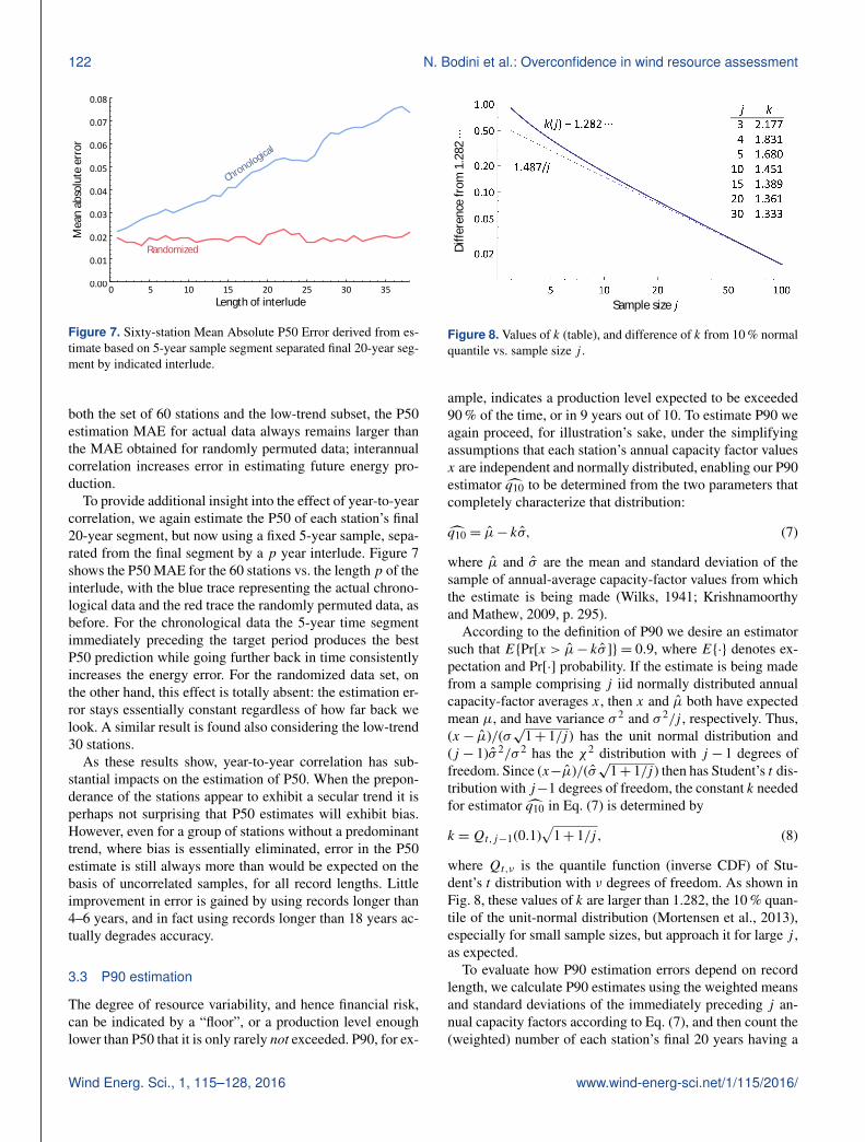
Figure 7. Sixty-station Mean Absolute P50 Error derived from es-timate based on 5-year sample segment separated final 20-year seg-ment by indicated interlude.

both the set of 60 stations and the low-trend subset, the P50estimation MAE for actual data always remains larger thanthe MAE obtained for randomly permuted data; interannualcorrelation increases error in estimating future energy pro-duction.

To provide additional insight into the effect of year-to-yearcorrelation, we again estimate the P50 of each station’s final20-year segment, but now using a fixed 5-year sample, sepa-rated from the final segment by a p year interlude. Figure 7shows the P50 MAE for the 60 stations vs. the length p of theinterlude, with the blue trace representing the actual chrono-logical data and the red trace the randomly permuted data, asbefore. For the chronological data the 5-year time segmentimmediately preceding the target period produces the bestP50 prediction while going further back in time consistentlyincreases the energy error. For the randomized data set, onthe other hand, this effect is totally absent: the estimation er-ror stays essentially constant regardless of how far back welook. A similar result is found also considering the low-trend30 stations.

As these results show, year-to-year correlation has sub-stantial impacts on the estimation of P50. When the prepon-derance of the stations appear to exhibit a secular trend it isperhaps not surprising that P50 estimates will exhibit bias.However, even for a group of stations without a predominanttrend, where bias is essentially eliminated, error in the P50estimate is still always more than would be expected on thebasis of uncorrelated samples, for all record lengths. Littleimprovement in error is gained by using records longer than4–6 years, and in fact using records longer than 18 years ac-tually degrades accuracy.

3.3 P90 estimation

The degree of resource variability, and hence financial risk,can be indicated by a “floor”, or a production level enoughlower than P50 that it is only rarely not exceeded. P90, for ex-

Sample size

Diffe

renc

e fr

om 1

.282

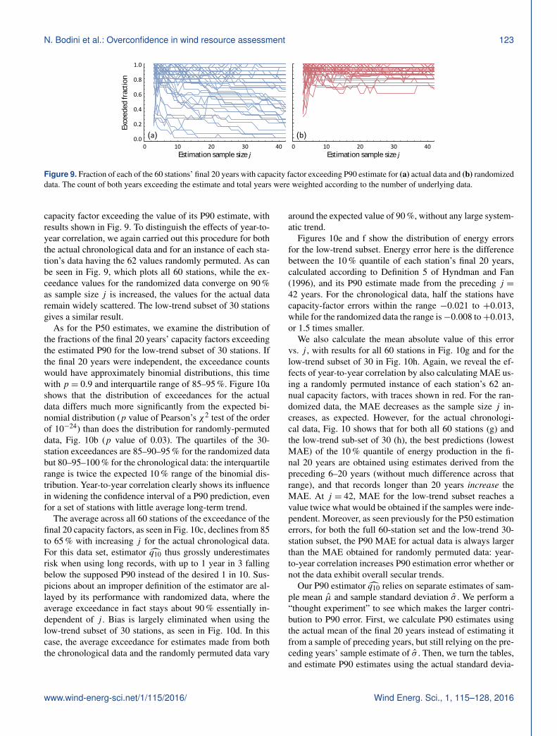
Figure 8. Values of k (table), and difference of k from 10 % normalquantile vs. sample size j .

ample, indicates a production level expected to be exceeded90 % of the time, or in 9 years out of 10. To estimate P90 weagain proceed, for illustration’s sake, under the simplifyingassumptions that each station’s annual capacity factor valuesx are independent and normally distributed, enabling our P90estimator q10 to be determined from the two parameters thatcompletely characterize that distribution:

q10 = µ− kσ, (7)

where µ and σ are the mean and standard deviation of thesample of annual-average capacity-factor values from whichthe estimate is being made (Wilks, 1941; Krishnamoorthyand Mathew, 2009, p. 295).

According to the definition of P90 we desire an estimatorsuch that E{Pr[x > µ− kσ ]} = 0.9, where E{·} denotes ex-pectation and Pr[·] probability. If the estimate is being madefrom a sample comprising j iid normally distributed annualcapacity-factor averages x, then x and µ both have expectedmean µ, and have variance σ 2 and σ 2/j , respectively. Thus,(x− µ)/(σ

√1+ 1/j ) has the unit normal distribution and

(j − 1)σ 2/σ 2 has the χ2 distribution with j − 1 degrees offreedom. Since (x−µ)/(σ

√1+ 1/j ) then has Student’s t dis-

tribution with j−1 degrees of freedom, the constant k neededfor estimator q10 in Eq. (7) is determined by

k =Qt,j−1(0.1)√

1+ 1/j, (8)

where Qt,ν is the quantile function (inverse CDF) of Stu-dent’s t distribution with ν degrees of freedom. As shown inFig. 8, these values of k are larger than 1.282, the 10 % quan-tile of the unit-normal distribution (Mortensen et al., 2013),especially for small sample sizes, but approach it for large j ,as expected.

To evaluate how P90 estimation errors depend on recordlength, we calculate P90 estimates using the weighted meansand standard deviations of the immediately preceding j an-nual capacity factors according to Eq. (7), and then count the(weighted) number of each station’s final 20 years having a

Wind Energ. Sci., 1, 115–128, 2016 www.wind-energ-sci.net/1/115/2016/

N. Bodini et al.: Overconfidence in wind resource assessment 123

(a)0.0

0.2

0.4

0.6

0.8

1.0

Exce

eded

frac

tion

0 10 20 30 40

Estimation sample size j

(b)0 10 20 30 40

Estimation sample size j

Figure 9. Fraction of each of the 60 stations’ final 20 years with capacity factor exceeding P90 estimate for (a) actual data and (b) randomizeddata. The count of both years exceeding the estimate and total years were weighted according to the number of underlying data.

capacity factor exceeding the value of its P90 estimate, withresults shown in Fig. 9. To distinguish the effects of year-to-year correlation, we again carried out this procedure for boththe actual chronological data and for an instance of each sta-tion’s data having the 62 values randomly permuted. As canbe seen in Fig. 9, which plots all 60 stations, while the ex-ceedance values for the randomized data converge on 90 %as sample size j is increased, the values for the actual dataremain widely scattered. The low-trend subset of 30 stationsgives a similar result.

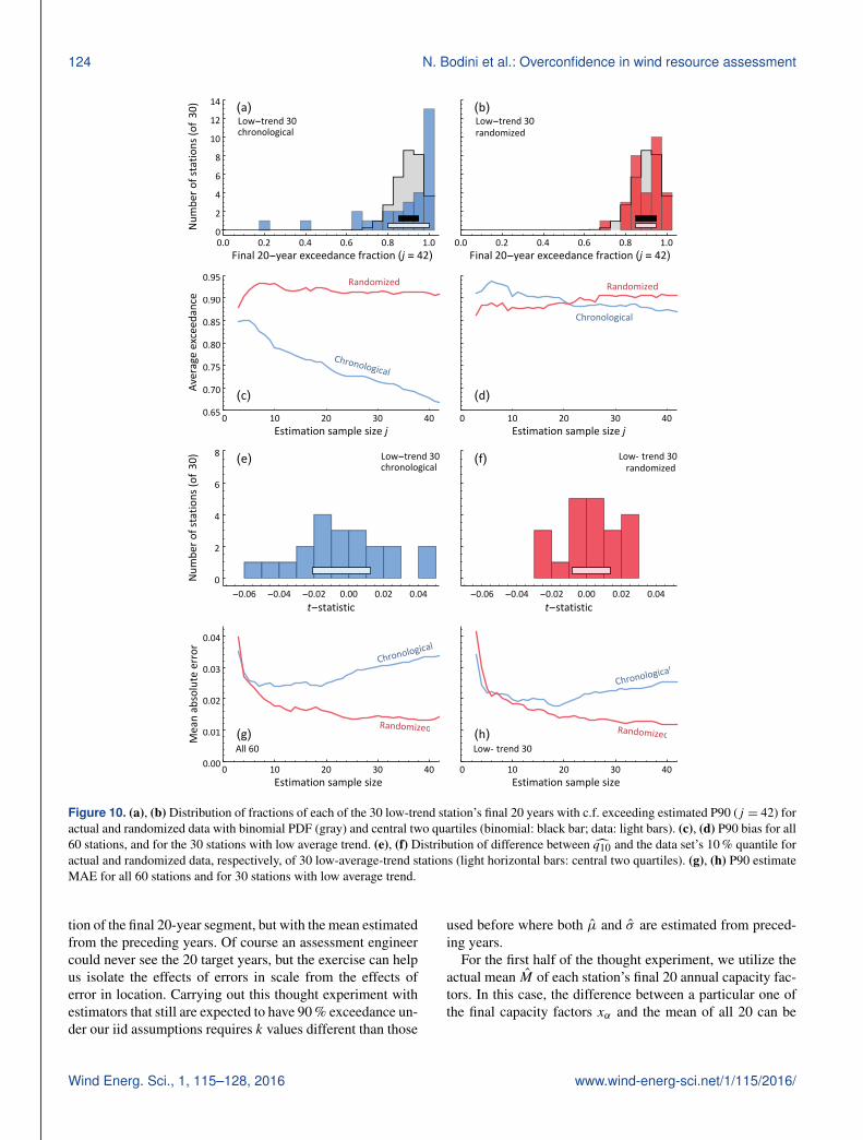
As for the P50 estimates, we examine the distribution ofthe fractions of the final 20 years’ capacity factors exceedingthe estimated P90 for the low-trend subset of 30 stations. Ifthe final 20 years were independent, the exceedance countswould have approximately binomial distributions, this timewith p = 0.9 and interquartile range of 85–95 %. Figure 10ashows that the distribution of exceedances for the actualdata differs much more significantly from the expected bi-nomial distribution (p value of Pearson’s χ2 test of the orderof 10−24) than does the distribution for randomly-permuteddata, Fig. 10b (p value of 0.03). The quartiles of the 30-station exceedances are 85–90–95 % for the randomized databut 80–95–100 % for the chronological data: the interquartilerange is twice the expected 10 % range of the binomial dis-tribution. Year-to-year correlation clearly shows its influencein widening the confidence interval of a P90 prediction, evenfor a set of stations with little average long-term trend.

The average across all 60 stations of the exceedance of thefinal 20 capacity factors, as seen in Fig. 10c, declines from 85to 65 % with increasing j for the actual chronological data.For this data set, estimator q10 thus grossly underestimatesrisk when using long records, with up to 1 year in 3 fallingbelow the supposed P90 instead of the desired 1 in 10. Sus-picions about an improper definition of the estimator are al-layed by its performance with randomized data, where theaverage exceedance in fact stays about 90 % essentially in-dependent of j . Bias is largely eliminated when using thelow-trend subset of 30 stations, as seen in Fig. 10d. In thiscase, the average exceedance for estimates made from boththe chronological data and the randomly permuted data vary

around the expected value of 90 %, without any large system-atic trend.

Figures 10e and f show the distribution of energy errorsfor the low-trend subset. Energy error here is the differencebetween the 10 % quantile of each station’s final 20 years,calculated according to Definition 5 of Hyndman and Fan(1996), and its P90 estimate made from the preceding j =42 years. For the chronological data, half the stations havecapacity-factor errors within the range −0.021 to +0.013,while for the randomized data the range is−0.008 to+0.013,or 1.5 times smaller.

We also calculate the mean absolute value of this errorvs. j , with results for all 60 stations in Fig. 10g and for thelow-trend subset of 30 in Fig. 10h. Again, we reveal the ef-fects of year-to-year correlation by also calculating MAE us-ing a randomly permuted instance of each station’s 62 an-nual capacity factors, with traces shown in red. For the ran-domized data, the MAE decreases as the sample size j in-creases, as expected. However, for the actual chronologi-cal data, Fig. 10 shows that for both all 60 stations (g) andthe low-trend sub-set of 30 (h), the best predictions (lowestMAE) of the 10 % quantile of energy production in the fi-nal 20 years are obtained using estimates derived from thepreceding 6–20 years (without much difference across thatrange), and that records longer than 20 years increase theMAE. At j = 42, MAE for the low-trend subset reaches avalue twice what would be obtained if the samples were inde-pendent. Moreover, as seen previously for the P50 estimationerrors, for both the full 60-station set and the low-trend 30-station subset, the P90 MAE for actual data is always largerthan the MAE obtained for randomly permuted data: year-to-year correlation increases P90 estimation error whether ornot the data exhibit overall secular trends.

Our P90 estimator q10 relies on separate estimates of sam-ple mean µ and sample standard deviation σ . We perform a“thought experiment” to see which makes the larger contri-bution to P90 error. First, we calculate P90 estimates usingthe actual mean of the final 20 years instead of estimating itfrom a sample of preceding years, but still relying on the pre-ceding years’ sample estimate of σ . Then, we turn the tables,and estimate P90 estimates using the actual standard devia-

www.wind-energ-sci.net/1/115/2016/ Wind Energ. Sci., 1, 115–128, 2016

124 N. Bodini et al.: Overconfidence in wind resource assessment

Low-trend 30chronological

(a)

0

2

4

6

8

10

12

14

Num

bero

fsta

tions

(of

30)

0.0 0.2 0.4 0.6 0.8 1.0Final 20-year exceedance fraction (j = 42)

Low-trend 30randomized

(b)

0.0 0.2 0.4 0.6 0.8 1.0Final 20-year exceedance fraction (j = 42)

Randomized

Chronological(c)0.65

0.70

0.75

0.80

0.85

0.90

0.95

Averageexceed

ance

0 10 20 30 40Estimation sample size j

Randomized

Chronological

(d)0 10 20 30 40

Estimation sample size j

Low-trend 30chronological

(e)

0

2

4

6

8

Num

bero

fsta

tions

(of

30)

-0.06 -0.04 -0.02 0.00 0.02 0.04t-statistic

Low- trend 30randomized

(f)

-0.06 -0.04 -0.02 0.00 0.02 0.04t-statistic

All 60

Randomized

Chronological

(g)0.00

0.01

0.02

0.03

0.04

Meanabsolute

error

0 10 20 30 40Estimation sample size

Low- trend 30

Randomized

Chronological

(h)0 10 20 30 40

Estimation sample size

Figure 10. (a), (b) Distribution of fractions of each of the 30 low-trend station’s final 20 years with c.f. exceeding estimated P90 (j = 42) foractual and randomized data with binomial PDF (gray) and central two quartiles (binomial: black bar; data: light bars). (c), (d) P90 bias for all60 stations, and for the 30 stations with low average trend. (e), (f) Distribution of difference between q10 and the data set’s 10 % quantile foractual and randomized data, respectively, of 30 low-average-trend stations (light horizontal bars: central two quartiles). (g), (h) P90 estimateMAE for all 60 stations and for 30 stations with low average trend.

tion of the final 20-year segment, but with the mean estimatedfrom the preceding years. Of course an assessment engineercould never see the 20 target years, but the exercise can helpus isolate the effects of errors in scale from the effects oferror in location. Carrying out this thought experiment withestimators that still are expected to have 90 % exceedance un-der our iid assumptions requires k values different than those

used before where both µ and σ are estimated from preced-ing years.

For the first half of the thought experiment, we utilize theactual mean M of each station’s final 20 annual capacity fac-tors. In this case, the difference between a particular one ofthe final capacity factors xα and the mean of all 20 can be

Wind Energ. Sci., 1, 115–128, 2016 www.wind-energ-sci.net/1/115/2016/

N. Bodini et al.: Overconfidence in wind resource assessment 125

All 60

Randomized

Chronological(a)

0.5

0.6

0.7

0.8

0.9

1.0

Aver

age

exce

edan

ce

0 10 20 30 40

Estimation sample size

Low- trend 30

Randomized

Chronological(b)

0 10 20 30 40

Estimation sample size

All 60

Randomized

Chronological

(c)

0.5

0.6

0.7

0.8

0.9

1.0

Aver

age

exce

edan

ce

0 10 20 30 40

Estimation sample size

Low- trend 30

Randomized

Chronological

(d)

0 10 20 30 40

Estimation sample size

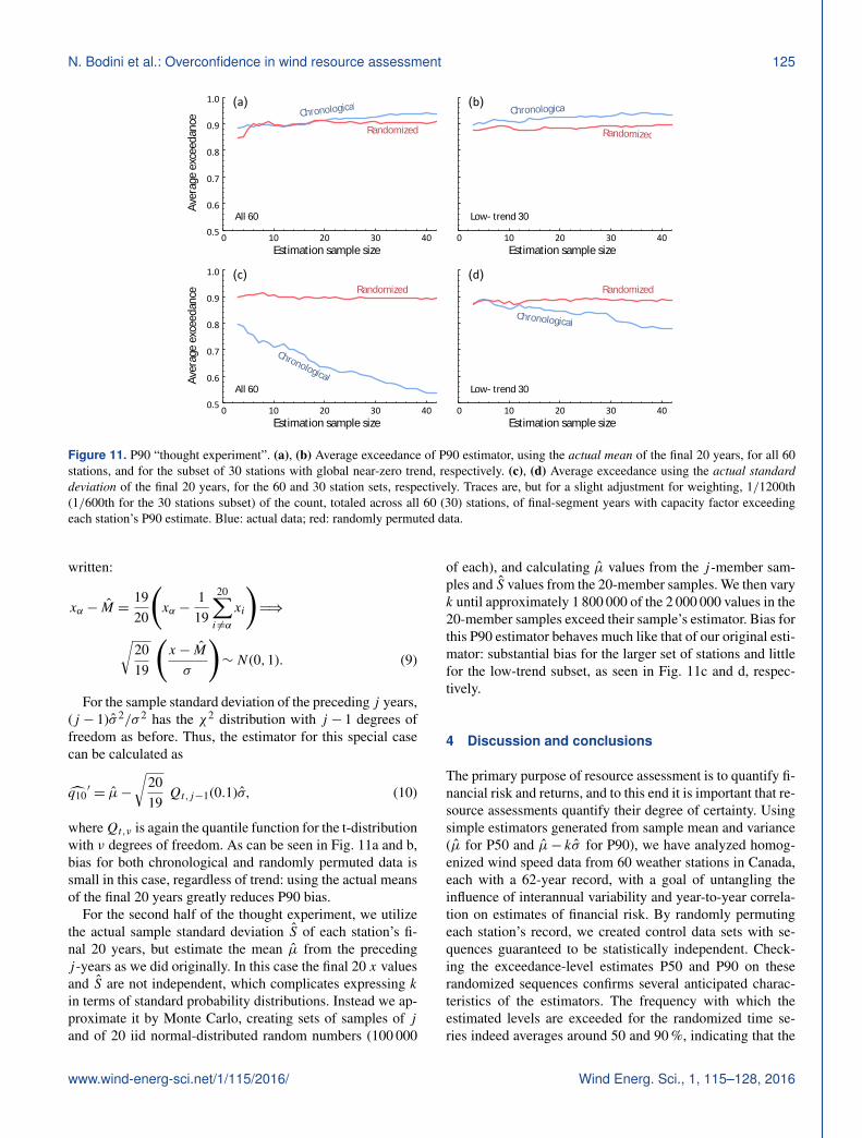
Figure 11. P90 “thought experiment”. (a), (b) Average exceedance of P90 estimator, using the actual mean of the final 20 years, for all 60stations, and for the subset of 30 stations with global near-zero trend, respectively. (c), (d) Average exceedance using the actual standarddeviation of the final 20 years, for the 60 and 30 station sets, respectively. Traces are, but for a slight adjustment for weighting, 1/1200th(1/600th for the 30 stations subset) of the count, totaled across all 60 (30) stations, of final-segment years with capacity factor exceedingeach station’s P90 estimate. Blue: actual data; red: randomly permuted data.

written:

xα − M =1920

(xα −

119

20∑i 6=α

xi

)H⇒

√2019

(x− M

σ

)∼N (0,1). (9)

For the sample standard deviation of the preceding j years,(j − 1)σ 2/σ 2 has the χ2 distribution with j − 1 degrees offreedom as before. Thus, the estimator for this special casecan be calculated as

q10′= µ−

√2019

Qt,j−1(0.1)σ, (10)

whereQt,ν is again the quantile function for the t-distributionwith ν degrees of freedom. As can be seen in Fig. 11a and b,bias for both chronological and randomly permuted data issmall in this case, regardless of trend: using the actual meansof the final 20 years greatly reduces P90 bias.

For the second half of the thought experiment, we utilizethe actual sample standard deviation S of each station’s fi-nal 20 years, but estimate the mean µ from the precedingj -years as we did originally. In this case the final 20 x valuesand S are not independent, which complicates expressing kin terms of standard probability distributions. Instead we ap-proximate it by Monte Carlo, creating sets of samples of jand of 20 iid normal-distributed random numbers (100 000

of each), and calculating µ values from the j -member sam-ples and S values from the 20-member samples. We then varyk until approximately 1 800 000 of the 2 000 000 values in the20-member samples exceed their sample’s estimator. Bias forthis P90 estimator behaves much like that of our original esti-mator: substantial bias for the larger set of stations and littlefor the low-trend subset, as seen in Fig. 11c and d, respec-tively.

4 Discussion and conclusions

The primary purpose of resource assessment is to quantify fi-nancial risk and returns, and to this end it is important that re-source assessments quantify their degree of certainty. Usingsimple estimators generated from sample mean and variance(µ for P50 and µ− kσ for P90), we have analyzed homog-enized wind speed data from 60 weather stations in Canada,each with a 62-year record, with a goal of untangling theinfluence of interannual variability and year-to-year correla-tion on estimates of financial risk. By randomly permutingeach station’s record, we created control data sets with se-quences guaranteed to be statistically independent. Check-ing the exceedance-level estimates P50 and P90 on theserandomized sequences confirms several anticipated charac-teristics of the estimators. The frequency with which theestimated levels are exceeded for the randomized time se-ries indeed averages around 50 and 90 %, indicating that the

www.wind-energ-sci.net/1/115/2016/ Wind Energ. Sci., 1, 115–128, 2016

126 N. Bodini et al.: Overconfidence in wind resource assessment

distributions of annual-average resource levels are approxi-mately normal, without much skew (which would bias sam-ple mean µ as an estimator of P50 or the resource median)or excess kurtosis (which would bias µ− kσ as an estima-tor P90 or the 10 % quantile). Hitting the target exceedancefrequency does require calculating k for the P90 estimatorfrom the t distribution. Improperly setting k = 1.282, the10 % quantile of the normal distribution, would give P88 es-timates when applied to samples of length j = 10, for exam-ple. With these P50 and P90 estimators, the mean absoluteenergy error (MAE) of the estimated capacity-factor quan-tiles falls monotonically with record length, as expected. Wechecked estimator performance by counting the number ofyears in the final 20 of each station’s record having a resourcelevel exceeding an estimate made from a preceding segmentof the record. When the estimation segment was substantiallylonger than 20 years the distribution of the count was essen-tially binomial with n= 20, and p = 0.5 or 0.9. These resultsshow that, save for the assumption of statistical independenceof the input data, the estimation methods are adequately for-mulated.

The performance of the estimators using the actual chrono-logical records is quite another story. When considering theentire set of 60 stations, both the P50 and P90 estimatesexhibited strong bias, grossly over-predicting resource lev-els actually attained in the final 20 years of each station’srecord. This bias is consistent with widespread decreasingwind speeds identified by Wan et al. (2010). Errors only fellwith record length for the first few preceding years (4 yearsfor P50 and 10 years for P90); for records longer than 5 years(P50) or 18 years (P90), error rose with sample length. Us-ing a sub-set of 30 stations contrived to have near-zero av-erage resource trend (same 30-station-average level for thefinal 20 years as for the preceding 20 years) essentially elim-inates estimation bias, but both energy and exceedance errorspreads increase with sample length for records longer than18 years, and are 2–3 times larger than either theoretical ex-pectations or errors obtained from the same estimation pro-cedures applied to randomized data. Thus, even absent over-all trends, year-to-year correlation in the chronological datareduces P50 and P90 certainty.

The higher errors of the estimates made from the chrono-logical data must arise from non-zero correlation (lack of sta-tistical independence) since these data are identical to therandomized control data except for sequence. One mighthope to account for the higher errors in estimates made fromthe correlated data in terms of an “effective number” of inde-pendent samples (Bayley and Hammersley, 1948; Corotis etal., 1977). For example, if the autocorrelation function of asequence of wind speed measurements was found to have anexponential form and to fall to 1/e in a lag time of τ = 6 h,then a sequence of hourly measurements having total dura-tion T � τ could be considered to comprise j = T/(2τ )=T/(12 h) independent samples, and confidence intervals forits mean value could be correctly estimated using this value

of j . However, this approach relies on the autocorrelationfunction having a finite sum or integral.

Previous work finds, though, that wind speeds seem to ex-hibit “long-term persistence”, with autocorrelation of a hy-perbolic form τ−α which cannot be summed. Wind’s persis-tence was first noted by Haslett and Raftery (1989) in theiranalysis of 18-year wind speed records from 12 stations inIreland. Subsequently Bakker and van den Hurk (2012) usedannual-mean geostrophic winds reconstructed from 12 sea-level pressure records with 75–126 year lengths, and foundstatistically significant persistence over the North Sea, GreatBritain and Ireland and along the Scandinavian coast. Sim-ilarly, Tsekouras and Koutsoyiannis (2014) analyzed 20 ob-servational wind-speed records from stations in Western Eu-rope, with record lengths ranging from 65 to 107 years,and found persistence in all. These findings place year-to-year correlations in wind-speed records in the same class asthose exhibited by river flows (Hurst, 1951) and a wide va-riety of other climatological (Pelletier and Turcotte, 1997;Koscielny-Bunde et al., 1998; Ault et al., 2013) and geo-physical (Witt and Malamud, 2013) processes. Our findings,that interannual wind speed variability (σ/µ) continues toincrease with segment length out to the 62-year limit of ourchronological data while for randomly permuted data it re-mains essentially constant, are also consistent with persis-tence. Because of the scale-free nature of the decay of persis-tent correlations, the effective number of independent sam-ples per unit record length does not approach a constant, andattempts to use this approach will “underrate uncertainty bya factor which tends to infinity with increasing number ofobservations” (Beran, 1989).

In light of the persistence behavior, it is premature to dis-miss the larger estimation errors from the 60-station set as be-ing somehow a spurious result attributable to nonstationarity.Persistent processes are characterized by seeming “trends”that spontaneously appear and disappear in a way that isactually entirely random (Beran et al., 2003, p. 3), makingit difficult to identify statistically significant “real” trends(Cohn and Lins, 2005). Will the “stilling” trends in ground-level wind speed observations (Klink, 2002; McVicar et al.,2008; Pryor et al., 2009; Vautard et al., 2010) reverse, in theway that “global dimming” has now become “global bright-ening” (Müller et al., 2014)? The increasing availability ofmulti-decade wind speed data sets, including the TwentiethCentury Reanalysis Project (Compo, 2011) in addition to theother multi-decadal works cited above, should enable an im-proved appraisal of the impact of trends on wind develop-ment risks.

We have shown here that year-to-year correlations in re-source level produce large effects, seemingly not recognizedor incorporated into current estimation practice, degradingthe certainty of pre-construction wind energy estimates. Forprimitive estimators, of the type utilized here, longer recordsdo not provide better estimates of future energy production.Since ignoring available data would not – and must not –

Wind Energ. Sci., 1, 115–128, 2016 www.wind-energ-sci.net/1/115/2016/

N. Bodini et al.: Overconfidence in wind resource assessment 127

be a reasonable solution, statistical approaches that explic-itly account for the observed year-to-year correlation shouldbe considered. One parsimonious approach would be to uti-lize estimation procedures based on long-term-persistencephenomenology, such as the pioneering comprehensive MCPtechnique proposed some time ago by Haslett and Raftery(1989). Given the distinctive nature of year-to-year changein the wind resource we further suggest that it might be pro-ductive to dissociate resource “variability” from instrumen-tal and model “uncertainty” in resource assessment presenta-tions.

5 Data availability

The homogenized monthly average windspeed source dataused in this work are freely available on the EnvironmentCanada website (Environment and Climate Change Canada,2016). The weighted annual-average capacity factors we de-rived from these data are available in the Supplementary Ma-terial here, along with a map showing locations of the 60selected Environment Canada stations.

The Supplement related to this article is available onlineat doi:10.5194/wes-1-115-2016-supplement.

Acknowledgements. We thank Environment Canada for makingthe monthly wind speed data used in this work openly accessible.Nicola Bodini was partially supported by a grant from OperaUniversitaria of Trento. This material is based upon work fundedby the National Science Foundation under Grant IIP-1332147. Theauthors appreciate helpful discussions with Jason Fields of theNational Renewable Energy Laboratory and with Chris Gifford ofDBRS Limited, Toronto.

Edited by: J. MannReviewed by: four anonymous referees

References

Albers, A.: Long term variation of wind potential: how long is longenough? presented at the DEWEK 2004: The International Tech-nical Wind Energy Conference, Wilhelmshaven, Germany, 2004.

Ault, T. R., Cole, J. E., Overpeck, J. T., Pederson, G. T., St. George,S., Otto-Bliesner, B., Woodhouse, C. A., and Deser, C.: TheContinuum of Hydroclimate Variability in Western North Amer-ica during the Last Millennium, J. Climate, 26, 5863–5878,doi:10.1175/jcli-d-11-00732.1, 2013.

Azorin-Molina, C., Vicente-Serrano, S. M., McVicar, T. R., Jerez,S., Sanchez-Lorenzo, A., López-Moreno, J.-I., Revuelto, J.,Trigo, R. M., Lopez-Bustins, J. A., and Espírito-Santo, F.: Ho-mogenization and Assessment of Observed Near-Surface WindSpeed Trends over Spain and Portugal, 1961–2011, J. Climate,27, 3692–3712, doi:10.1175/jcli-d-13-00652.1, 2014.

Bakker, A. R. and van den Hurk, B. J. J. M.: Estimation of persis-tence and trends in geostrophic wind speed for the assessmentof wind energy yields in Northwest Europe, Clim. Dynam., 39,767–782, doi:10.1007/s00382-011-1248-1, 2012.

Bayley, G. V. and Hammersley, J. M.: The “Effective” Numberof Independent Observations in an Autocorrelated Time Series,Supplement to the Journal of the Royal Statistical Society, 8,184–197, doi:10.2307/2983560, 1946.

Beran, J.: A test of location for data with slowly de-caying serial correlations, Biometrika, 76, 261–269,doi:10.1093/biomet/76.2.261, 1989.

Beran, J., Feng, Y., Ghosh, S., and Kulik, R.: Long-MemoryProcesses: Probabilistic Properties and Statistical Methods,Springer, doi:10.1007/978-3-642-35512-7, 2013.

Bett, P. E., Thornton, H. E., and Clark, R. T.: European wind vari-ability over 140 yr, Adv. Sci. Res., 10, 51–58, doi:10.5194/asr-10-51-2013, 2013.

Bett, P. E., Thornton, H. E., and Clark, R. T.: Using theTwentieth Century Reanalysis to assess climate variability forthe European wind industry, Theor. Appl. Climatol., 1–20,doi:10.1007/s00704-015-1591-y, 2015.

Brower, M. C.: Wind Resource Assessment: A Practical Guide toDeveloping a Wind Project, John Wiley & Sons, 2012.

Carta, J. A., Velázquez, S., and Cabrera, P.: A review of measure-correlate-predict (MCP) methods used to estimate long-termwind characteristics at a target site, Renew. Sust. Energ. Rev.,27, 362–400, doi:10.1016/j.rser.2013.07.004, 2013.

Cohn, T. A. and Lins, H. F.: Nature’s style: Naturally trendy, Geo-phys. Res. Lett., 32, L23402, doi:10.1029/2005gl024476, 2005.

Compo, G. P., Whitaker, J. S., Sardeshmukh, P. D., Matsui, N., Al-lan, R. J., Yin, X., Gleason, B. E., Vose, R. S., Rutledge, G.,Bessemoulin, P., Brönnimann, S., Brunet, M., Crouthamel, R. I.,Grant, A. N., Groisman, P. Y., Jones, P. D., Kruk, M. C., Kruger,A. C., Marshall, G. J., Maugeri, M., Mok, H. Y., Nordli, Ø., Ross,T. F., Trigo, R. M., Wang, X. L., Woodruff, S. D., and Worley, S.J.: The Twentieth Century Reanalysis Project, Q. J. Roy. Me-teor. Soc., 137, 1–28, doi:10.1002/qj.776, 2011.

Corotis, R. B.: Confidence interval procedures for wind turbinecandidate sites, Sol. Energ., 24, 427–433, doi:10.1016/0038-092X(80)90310-2, 1980.

Corotis, R. B., Sigl, A. B., and Cohen, M. P.: VarianceAnalysis of Wind Characteristics for Energy Conversion,J. Appl. Meteorol., 16, 1149–1157, doi:10.1175/1520-0450(1977)016<1149:vaowcf>2.0.co;2, 1977.

Earl, N., Dorling, S., Hewston, R., and von Glasow, R.: 1980–2010Variability in U.K. Surface Wind Climate, J. Climate, 26, 1172–1191, doi:10.1175/jcli-d-12-00026.1, 2012.

Environment and Climate Change Canada: Historical and Homog-enized surface wind speeds for Canada. Update to Decem-ber 2014, https://www.ec.gc.ca/dccha-ahccd/default.asp?lang=En&n=552AFB3E-1, last access: 21 February 2016.

Früh, W. G.: Long-term wind resource and uncertainty estimationusing wind records from Scotland as example, Renew. Energ.,50, 1014–1026, doi:10.1016/j.renene.2012.08.047, 2013.

Haslett, J. and Raftery, A. E.: Space-time modelling with long-memory dependence: assessing Ireland’s wind power resource,J. Roy. Stat. Soc. C-App., 38, 1–50, doi:10.2307/2347679, 1989.

Hurst, H. E.: Long-term storage capacity of reservoirs,Trans. Am. Soc. Civ. Eng., 116, 770–808, 1951.

www.wind-energ-sci.net/1/115/2016/ Wind Energ. Sci., 1, 115–128, 2016

128 N. Bodini et al.: Overconfidence in wind resource assessment

Hyndman, R. J. and Fan, Y.: Sample Quantiles in Statistical Pack-ages, Am. Stat., 50, 361–365, doi:10.2307/2684934, 1996.

Justus, C. G., Mani, K., and Mikhail, A. S.: Interannual and Month-to-Month Variations of Wind Speed, J. Appl. Meteorol., 18, 913–920, doi:10.1175/1520-0450(1979)018<0913:iamtmv>2.0.co;2,1979.

Kenney, J. F.: Mathematics of Statistics. Part II, Chapman and Hall,London, 1940.

Kirchner-Bossi, N., García-Herrera, R., Prieto, L., and Trigo, R.M.: A long-term perspective of wind power output variability,Int. J. Climatol., 35, 2635–2646, doi:10.1002/joc.4161, 2015.

Klink, K.: Trends and Interannual Variability of Wind SpeedDistributions in Minnesota, J. Climate, 15, 3311–3317,doi:10.1175/1520-0442(2002)015<3311:TAIVOW>2.0.CO;2,2002.

Klink, K.: Atmospheric Circulation Effects on Wind Speed Vari-ability at Turbine Height, J. Appl. Meteorol. Clim., 46, 445–456,doi:10.1175/jam2466.1, 2007.

Koscielny-Bunde, E., Bunde, A., Havlin, S., Roman, H. E., Gol-dreich, Y., Schellnhuber, H.-J.: Indication of a Universal Persis-tence Law Governing Atmospheric Variability, Phys. Rev. Lett.,81, 729–732, doi:10.1103/PhysRevLett.81.729, 1998.

Krishnamoorthy, K. and Mathew, T.: Statistical Tolerance Regions.Theory, Applications, and Computation, John Wiley & Sons,Hoboken, 2009.

Lackner, M. A., Rogers, A. L., and Manwell, J. F.: UncertaintyAnalysis in MCP-Based Wind Resource Assessment and En-ergy Production Estimation, J. Sol. Energy Eng., 130, 031006–031006, doi:10.1115/1.2931499, 2008.

Landberg, L., Myllerup, L., Rathmann, O., Petersen, E. L., Jør-gensen, B. H., Badger, J., and Mortensen, N. G.: Wind Re-source Estimation – An Overview, Wind Energy, 6, 261–271,doi:10.1002/we.94, 2003.

McVicar, T. R., Van Niel, T. G., Li, L. T., Roderick, M. L.,Rayner, D. P., Ricciardulli, L., and Donohue, R. J.: Windspeed climatology and trends for Australia, 1975–2006: Cap-turing the stilling phenomenon and comparison with near-surface reanalysis output, Geophys. Res. Lett., 35, L20403,doi:10.1029/2008gl035627, 2008.

Mortensen, N. G. and Jørgensen, H. E.: Comparative Resourceand Energy Yield Assessment Procedures (CREYAP) Pt. II, pre-sented at EWEA Technology Workshop: Resource Assessment2013, Dublin, available at: http://orbit.dtu.dk/files/70667004/Comparative_Resource_and_Energy_Yield.pdf (last access: 18August 2016), 2013.

Müller, B., Wild, M., Driesse, A., and Behrens, K.: Re-thinking solar resource assessments in the context ofglobal dimming and brightening, Sol. Energ., 99, 272–282,doi:10.1016/j.solener.2013.11.013, 2014.

Palutikof, J. P., Davies, T. D., and Kelly, P. M.: An analysis of sevenlong-term wind-speed records of the British Isles with particu-lar reference to the implications for wind power production, in:Wind energy conversion, 1985: Proceedings of the 7th BritishWind Energy Association Conference, edited by: Garrad, A.,Mechanical Engineering Publications, Ltd, 235–240, 1985.

Palutikof, J. P., Guo, X., and Halliday, J. A.: Climate variability andthe UK wind resource, J. Wind Eng. Ind. Aerod., 39, 243–249,doi:10.1016/0167-6105(92)90550-T, 1992.

Pelletier, J. D. and Turcotte, D. L.: Long-range persistence in cli-matological and hydrological time series: analysis, modeling andapplication to drought hazard assessment, J. Hydrol., 203, 198–208, doi:10.1016/S0022-1694(97)00102-9, 1997.

Pryor, S. C. and Ledolter, J.: Addendum to “Wind speed trends overthe contiguous United States”, J. Geophys. Res.-Atmos., 115,D10103, doi:10.1029/2009jd013281, 2010.

Pryor, S. C., Barthelmie, R. J., Young, D. T., Takle, E. S., Arritt, R.W., Flory, D., Gutowski, W. J., Nunes, A., and Roads, J.: Windspeed trends over the contiguous United States, J. Geophys. Res.-Atmos., 114, D14105, doi:10.1029/2008jd011416, 2009.

Rose, S. and Apt, J.: What can reanalysis data tell usabout wind power?, Renew. Energ., 83, 963–969,doi:10.1016/j.renene.2015.05.027, 2015.

Rose, S. and Apt, J.: Quantifying sources of uncertainty in re-analysis derived wind speed, Renew. Energ., 94, 157–165,doi:10.1016/j.renene.2016.03.028, 2016.

Salmon, J. and Taylor, P.: Errors and uncertainties associated withmissing wind data and short records, Wind Energy, 17, 1111–1118, doi:10.1002/we.1613, 2014.

St. Martin, C. M., Lundquist, J. K., and Handschy, M. A.: Variabilityof interconnected wind plants: correlation length and its depen-dence on variability time scale, Environ. Res. Lett., 10, 044004,doi:10.1088/1748-9326/10/4/044004, 2015.

Tsekouras, G. and Koutsoyiannis, D.: Stochastic analysis andsimulation of hydrometeorological processes associatedwith wind and solar energy, Renew. Energ., 63, 624-633,doi:10.1016/j.renene.2013.10.018, 2014.

Vautard, R., Cattiaux, J., Yiou, P., Thepaut, J.-N., and Ciais, P.:Northern Hemisphere atmospheric stilling partly attributed toan increase in surface roughness, Nat. Geosci., 3, 756–761,doi:10.1038/ngeo979, 2010.

Walter, K., Weiss, C. C., Swift, A. H. P., Chapman, J., and Kel-ley, N. D.: Speed and Direction Shear in the Stable NocturnalBoundary Layer, J. Sol. Energy Eng., 131, 011013-1–011013-7,doi:10.1115/1.3035818, 2009.

Wan, H., Wang, X. L., and Swail, V. R.: Homogenization and trendanalysis of Canadian near-surface windspeeds, J. Climate, 23,1209–1225, doi:10.1175/2009jcli3200.1, 2010.

Watson, S. J., Kritharas, P., and Hodgson, G. J.: Wind speed vari-ability across the UK between 1957 and 2011, Wind Energy, 18,21–42, doi:10.1002/we.1679, 2015.

Wilks, S. S.: Determination of sample sizes for set-ting tolerance limits, Ann. Math. Stat., 12, 91–96,doi:10.1214/aoms/1177731788, 1941.

Witt, A. and Malamud, B.: Quantification of Long-Range Persis-tence in Geophysical Time Series: Conventional and Benchmark-Based Improvement Techniques, Surv. Geophys., 34, 541–651,doi:10.1007/s10712-012-9217-8, 2013.

Wind Energ. Sci., 1, 115–128, 2016 www.wind-energ-sci.net/1/115/2016/