Yashar Ganjali

High Performance Networking GroupStanford University

September 17, 2003

Minimum-delay RoutingMinimum-delay Routing

February 13, 2003 Minimum-delay Routing 2

Outline1. Network and flow model2. Delay model3. Problem statement4. Previous work5. New algorithm6. A simple example7. Outline of the optimality proof

February 13, 2003 Minimum-delay Routing 3

Network & Flow Model

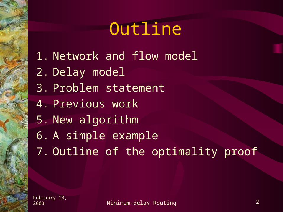
• Network G=(V,E)– N nodes– M links

• K commodities– Source si

– Destination ti

– Demand di s1

t1

s2

s3

t2

t3

d1

February 13, 2003 Minimum-delay Routing 4

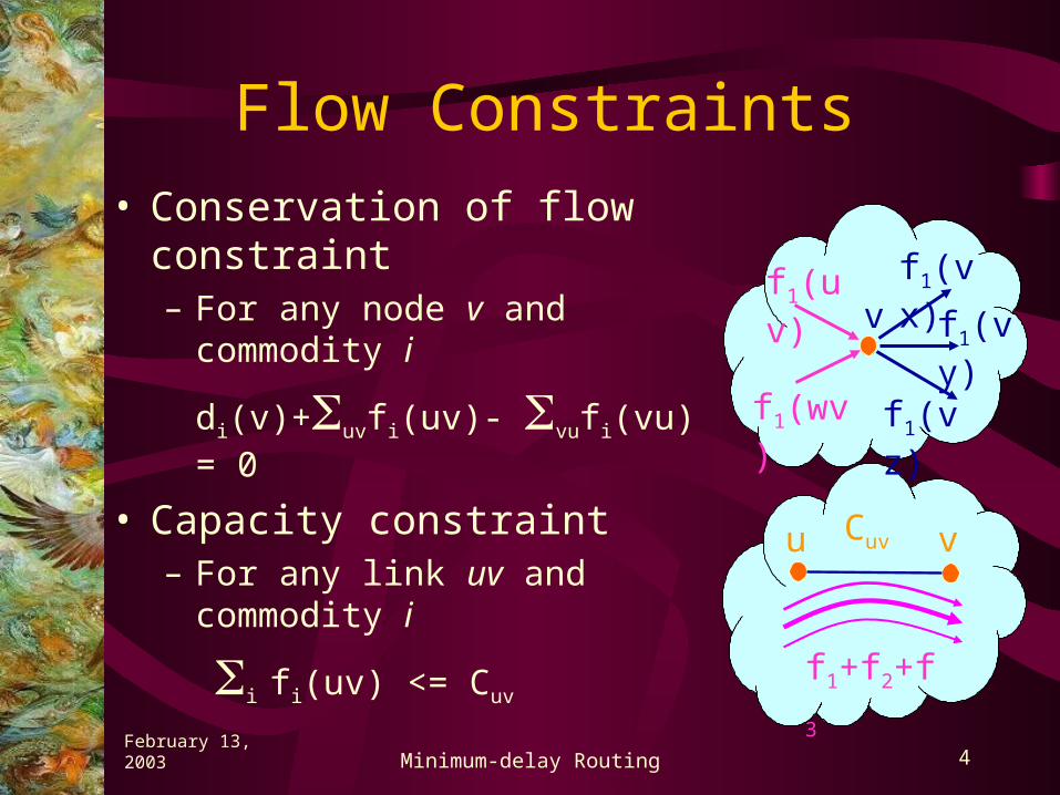
Flow Constraints• Conservation of flow

constraint– For any node v and

commodity i

di(v)+uvfi(uv)- vufi(vu) = 0

• Capacity constraint– For any link uv and

commodity i

i fi(uv) <= Cuv

u vCuv

f1+f2+f3

f1(uv)f1(vx)

f1(wv)

f1(vy)

f1(vz)

v

February 13, 2003 Minimum-delay Routing 5

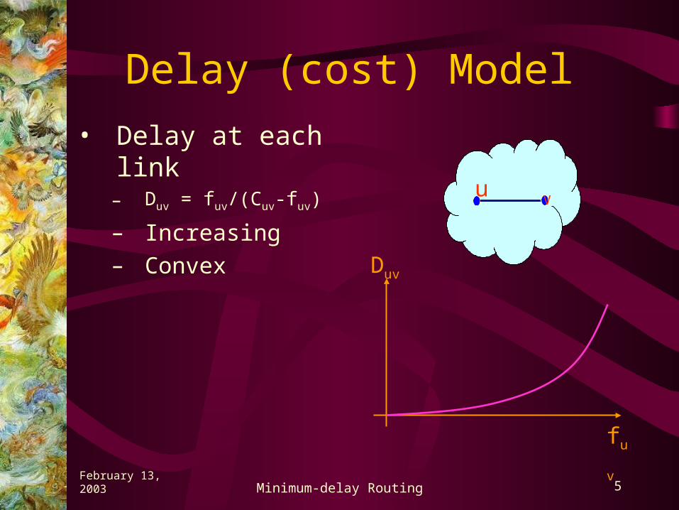
Delay (cost) Model• Delay at each link

– Duv = fuv/(Cuv-fuv)

– Increasing– Convex

uV

fuv

Duv

February 13, 2003 Minimum-delay Routing 6

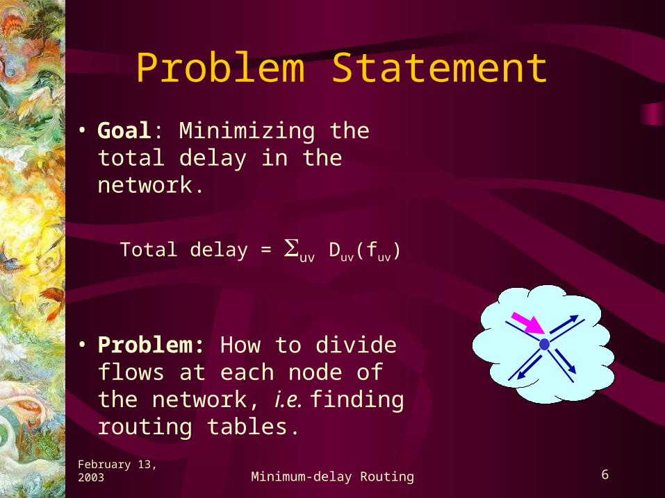
Problem Statement• Goal: Minimizing the total

delay in the network.

Total delay = uv Duv(fuv)

• Problem: How to divide flows at each node of the network, i.e. finding routing tables.

February 13, 2003 Minimum-delay Routing 7

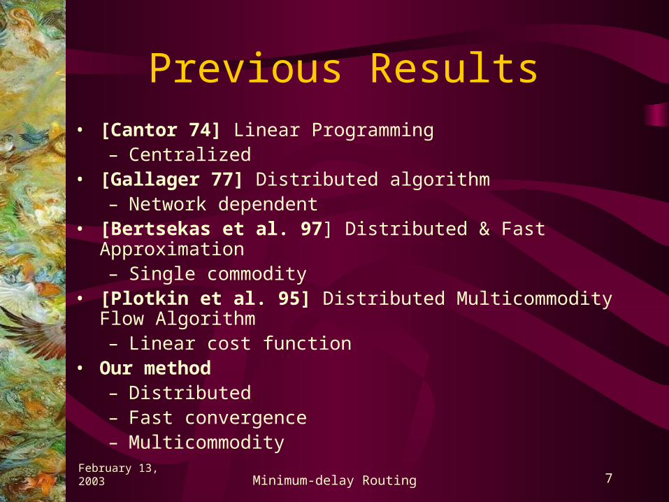
Previous Results• [Cantor 74] Linear Programming

– Centralized• [Gallager 77] Distributed algorithm

– Network dependent• [Bertsekas et al. 97] Distributed & Fast Approximation

– Single commodity• [Plotkin et al. 95] Distributed Multicommodity Flow

Algorithm– Linear cost function

• Our method– Distributed– Fast convergence– Multicommodity

February 13, 2003 Minimum-delay Routing 8

Relaxing Conservation of Flow Constraint

• We relax the conservation of flow constraint:

di(v)+uvfi(uv)- vufi(vu) = gi(f,v)

• We call gi(f,v) the excess of commodity i at node v and flow f is called a pre-flow.

• We will use this quantity to find points of high pressure in the network.

February 13, 2003 Minimum-delay Routing 9

Minimum-delay RoutingPotential Function

• We define 1 = uv,iexp(gi(f,uv)/di)

and 2 = uv Duv(fuv )/B

1 measures how close the current pre-flow f is to a flow.

2 measures how close the cost of the current flow is to the budget B.

• We let = 1 + 1 x2

February 13, 2003 Minimum-delay Routing 10

Minimum-delay algorithm: Starting from zero flows our goals is to minimize

O(-1log(m-1)) phases

O(-1) iterations– Increase capacities by a factor of – Increase demands by a factor of – Update the amount of excess at each node– BALANCE EXCESSES

• Rescale capacities and demands• Update if needed

Our Algorithm

February 13, 2003 Minimum-delay Routing 11

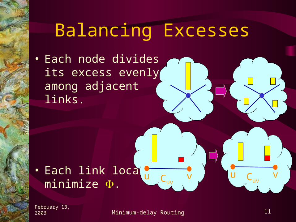
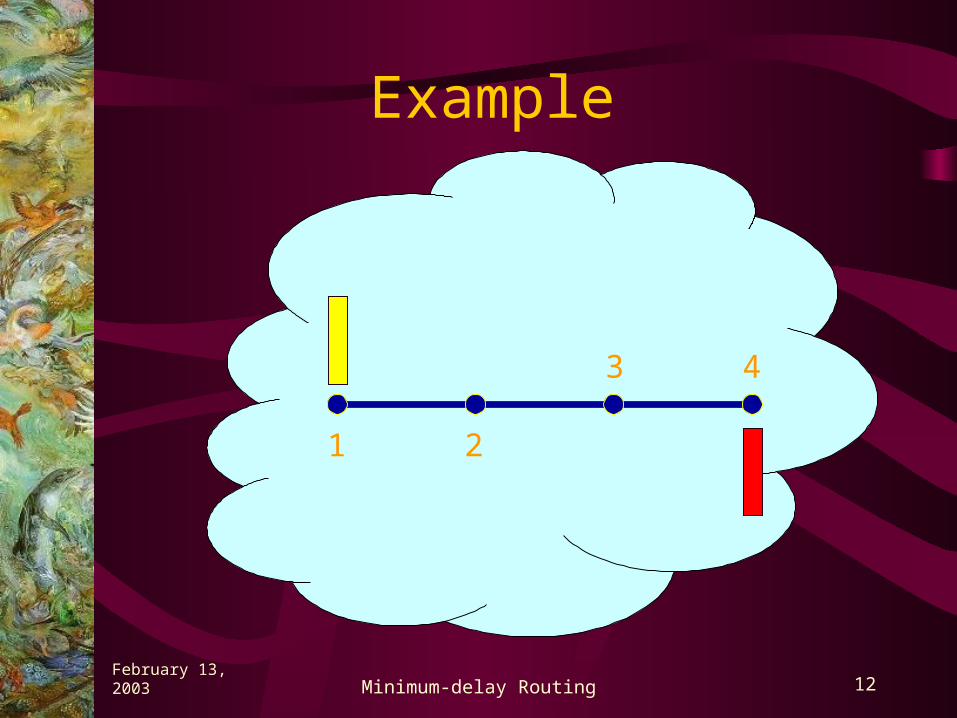
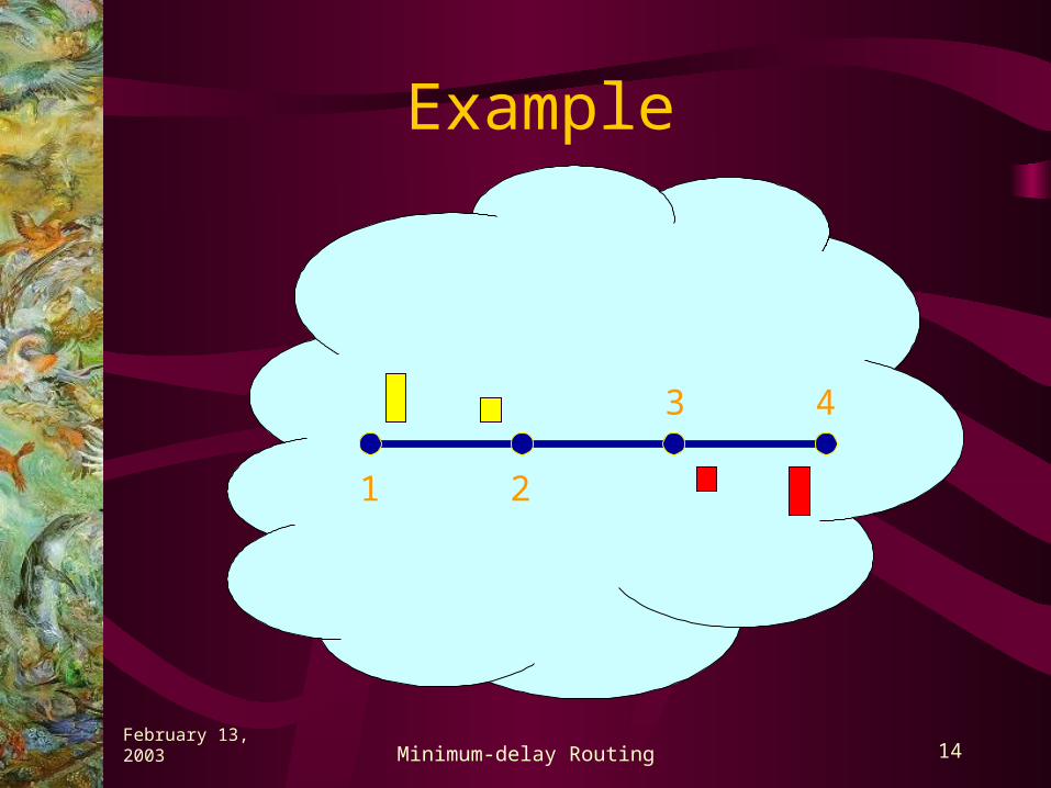
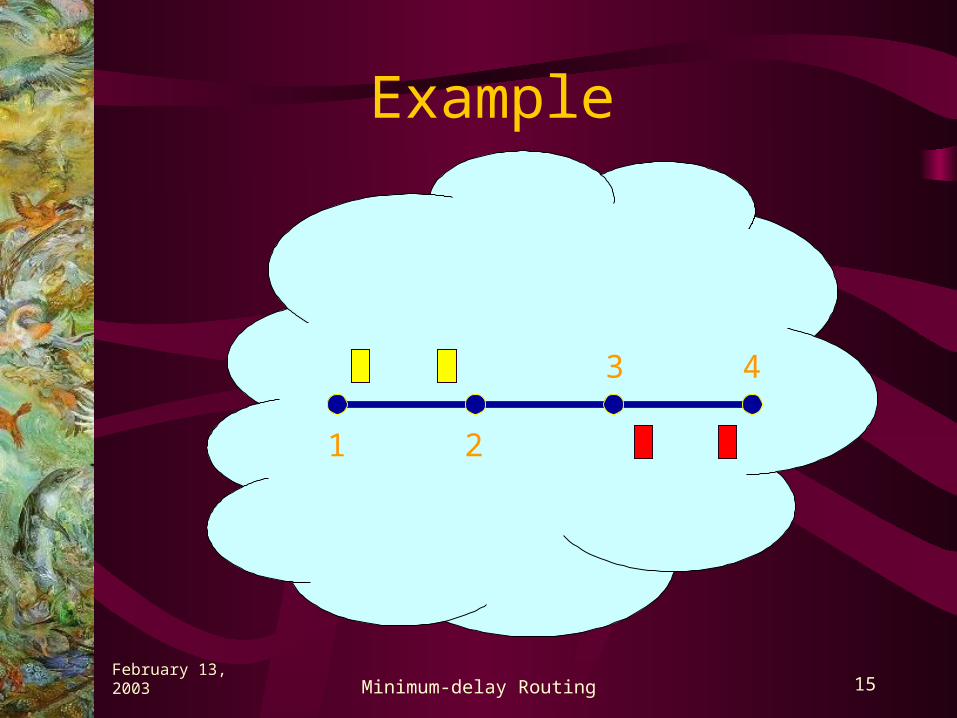
Balancing Excesses• Each node divides

its excess evenly among adjacent links.

• Each link locally minimize . u vCuv

u vCuv

February 13, 2003 Minimum-delay Routing 12

Example

1 2

3 4

February 13, 2003 Minimum-delay Routing 13

Example

1 2

3 4

February 13, 2003 Minimum-delay Routing 14

Example

1 2

3 4

February 13, 2003 Minimum-delay Routing 15

Example

1 2

3 4

February 13, 2003 Minimum-delay Routing 16

Outline of the Proof

1. If is small enough we are close to the optimal solution.

2. In each ITERATION the increase in is small.

3. At the end of each PHASE the amount of is divided by two.

February 13, 2003 Minimum-delay Routing 17

Small Close to Optimal

• We know = 1 + …x 2

is small means both 1 and 2 are small. 1 is small means conservation of flows is

almost satisfied. 2 is small means cost is close to optimal.

• We can show that if < (1+) at least (1-) of each demand is satisfied and our cost is at most (1+) times the optimal cost

February 13, 2003 Minimum-delay Routing 18

Increase in is small• Consider an optimal flow f*• We have f* <= C and f* <= C• Therefore, in each iteration we can

have f = f* • We can show the increase in is small

in this case (cost function is convex and has a bounded derivative).

• Therefore, if we minimize the amount of increase is small.

February 13, 2003 Minimum-delay Routing 19

In each phase decreases

by a factor < 1• At the end of each phase we divide all demands and flows by two.

• Therefore excesses and delays are reduced.

• We can show this reduces by a factor which is less than 1.

February 13, 2003 Minimum-delay Routing 20

Complexity of the Algorithm

• Original is bounded.• We know is multiplied by a factor

less than one in each phase.• We can conclude that the algorithm

has O(-1log(m-1)) phases.• Each phase consists of O(-1)

iterations.

• Running Time: O*(-2-2KM2N)• Improved running time: O*(-3-3KMN2)

February 13, 2003 Minimum-delay Routing 21

Future Work• Sensitivity and stability analysis

– How sensitive the algorithm is to perturbations?

• Cost function– Realistic cost function

• Implementations issues– Where?– How to incorporate with existing routing protocols?

February 13, 2003 Minimum-delay Routing 22

Thank you!Thank you!