EE 552, Exam 2, Take-home. Due Monday, April 11, 2016, 5:00pm. You may use class notes or any

reference materials (e.g., books, etc.) that you like; however, you must work alone, i.e., you should

not be communicating with anyone else about how to work the problems on this exam.

1. Generation planning (25 pts): Develop the complete set of equations for generation expansion

plan formulation 11-b (GEP-11b), based on the following data and assumptions.

a. Plan for 30 years, at 5 year intervals (thus you should have 6 investment periods (at years

5, 10, 15, 20, 25, and 30).

b. Use annual discount rate of 9%.

c. Maintain a reserve of 15% above peak load.

d. Assume a CO2 cost of $25/MT (you will need to add a term to the objective function to

account for this).

e. Transmission topology and data: Two comments follow…

Note the definitions of positive branch flow for each Pbk, k=1,…,5.

The admittances yij are given on a 100 MVA power base.

y13 =-j10 y14 =-j10

y34 =-j10

y23 =-j10

y12 =-j10

Pg1

Pd3

Pd2

1 2

3 4

Pg2

Pg4

Pb1

Pb3

Pb3

Pb4

Pb5

f. Line flow constraints: -500MW≤Pbk≤5000MW, k=1,5. The per-unit expressions of these

constraints, on a 100 MVA power base, are -500≤Pbk≤500. Given the level of loads (see

item (j) below), this implies the transmission has infinite capacity.

g. Existing generation data: Bus 1 Bus 2 Bus 4

Technology PC (j=1) NGCC (j=3) CT (j=4)

Capacity (MW) 100 100 50

h. Technology characteristics PC (j=1) PC (j=2) NGCC(j=3) CT (j=4) Wind (j=5)

Capacity credit 1.0 1.0 1.0 1.0 0.15

Investment cost (1000$/MW) 3000 2917 912 968 1980

Fixed O&M costs (1000$/MW/yr) 50 31 13 7 40

Var O&M ($/MWhr) 10 4.5 3.6 15.5 0

Full-load heat rate (MBTU/MWhr) 10.0 8.8 7.05 10.8 --

Fuel cost ($/MBTU) 3 3 4 4 0

CO2 emissions (lbs/MWhr) 2120 1872 825 1264 0

Capacity factor 1 1 1 1 0.35

Salvage value (1000$/MW) 50 50 40 20 0

i. Load duration curve and corresponding blocks. Assume a load growth rate of 2%/year,

applied to each value d1, d2, d3, for each of the two loads in the system, with the durations

h1, h2, and h3 remaining the same. Therefore, for example, for the load at bus 2, d1 would

be 1.0, 1.0824, 1.1951, 1.3195, 1.4568, 1.6084, 1.7758 pu for years 1, 5, 10, 15, 20, 25,

and 30, respectively. You will need to compute the values of d2 and d3 for these years as

well. Then you will need to do the same for the load at bus 3.

Number of hours that Load > L

L

(M

W)

d1

d2

d3

h1 h1+h2 h1+h2+h3

Initial load at bus 2 (Pg2)

Block 1 Block 2 Block 3

Load (pu) d1=1 d2=0.8 d3=0.6

Duration (hrs) h1=1000 h2=5000 h3=2760

Initial load at bus 3 (Pg3)

Block 1 Block 2 Block 3

Load (pu) d1=1.1 d2=0.9 d3=0.7

Duration (hrs) h1=900 h2=5200 h3=2660

2. Production costing (22 pts):

a. (4 pts) A load duration curve characterizes the next year for a power system is given below.

The power system is supplied by one 3 MW unit. Identify the minimum load, the loss of

load probability, the loss of load expectation, and the expected unserved energy, assuming

the 3 MW unit is perfectly reliable.

)( eD dFr

1

1 2 3 4 5 6 7 8

0.8

0.6

0.4

0.2 de (MW)

Solution:

Minimum Load=1 MW, LOLP=P(d>3)=0.333, LOLE=0.333*8760=2917 hrs

EUE=Area*T=0.5(1)(.333)(8760)=0.1666(8760)=1460MWhrs

b. (5 pts) Now consider that the power system is supplied with one 4 MW unit having a forced

outage rate of 0.25. The load is still characterized by the load duration curve above.

Compute loss of load probability, loss of load expectation, and expected unserved energy.

Solution:

)()1(

eDdF

r

* 1

1 2 3 4 5 6 7 8

C1=4

0.8

0,6

0.4

0.2

1.

1 2 3 4 5 6 7 8 de

0.8

0.6

0.4

0.2

+

1.

1 2 3 4 5 6 7 8 de

0.8

0.6

0.4

0.2

1.0

1 2 3 4 5 6 7 8 de

0.8

0.6

0.4

0.2

=

(c) (d)

(e)

(b)

fDj(dj)

)( eD dFr

1

1 2 3 4 5 6 7 8

0.8

0.6

0.4

0.2 de (MW)

0.75

0.25

0.75

0.25

So

LOLP=P(d>4)=0.25, LOLE=0.25*8760=2190hrs

EUE=8760{(1)(0.25)+0.5(3)(0.25)}=8760{.25+.375}=5475MWhrs

c. (3 pts) Consider the two situations you have assessed in parts (a) and (b) of this problem.

Complete the following sentence:

Although situation ____ has the larger LOLP; situation ____ has the larger EUE because

_____________________________________________________________

______________________________________________________________

______________________________________________________________

______________________________________________________________.

Solution:

Although situation (a) has a larger LOLP, situation (b) has a larger EUE because when load is

interrupted in situation (a), it will only be for 0 to 1 MW, whereas when load is interrupted in

situation (b), it will be for 0 to 4 MW.

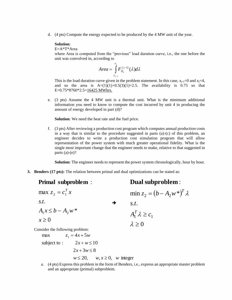
d. (4 pts) Compute the energy expected to be produced by the 4 MW unit of the year.

Solution:

E=A*T*Area

where Area is computed from the “previous” load duration curve, i.e., the one before the

unit was convolved in, according to

dFArea

j

j

e

x

x

j

D

1

)()1(

This is the load duration curve given in the problem statement. In this case, xj-1=0 and xj=4,

and so the area is A=(1)(1)+0.5(3)(1)=2.5. The availability is 0.75 so that

E=0.75*8760*2.5=16425 MWhrs.

e. (3 pts) Assume the 4 MW unit is a thermal unit. What is the minimum additional

information you need to know to compute the cost incurred by unit 4 in producing the

amount of energy developed in part (d)?

Solution: We need the heat rate and the fuel price.

f. (3 pts) After reviewing a production cost program which computes annual production costs

in a way that is similar to the procedure suggested in parts (a)-(c) of this problem, an

engineer decides to write a production cost simulation program that will allow

representation of the power system with much greater operational fidelity. What is the

single most important change that the engineer needs to make, relative to that suggested in

parts (a)-(e)?

Solution: The engineer needs to represent the power system chronologically, hour by hour.

3. Benders (17 pts): The relation between primal and dual optimizations can be stated as:

0

*

..

max

:

21

12

x

wAbxA

ts

xcz T

subproblem Primal

0

..

*min

:

11

22

cA

ts

wAbz

T

T

subproblem Dual

Consider the following problem:

integer 0,,,20

832

102 :subject to

54 max 1

wxww

wx

wx

wxz

a. (4 pts) Express this problem in the form of Benders, i.e., express an appropriate master problem

and an appropriate (primal) subproblem.

Solution:

Master problem:

integer ,0,,20 :Qs.t

5z max

*

2

*

21

wwMzw

zw

Subproblem:

0

382

102 subject to

4 max 2

x

wx

wx

xz

b. (3 pts) Identify an initial solution to the master.

Solution:

20,*

2 wMz

c. (4 pts) Formulate the subproblem dual in terms of w*, and based on the dual formulation, and

the solution to the master problem found in part (b), explain why you know that the primal

subproblem is infeasible.

Solution: We first express the subproblem dual.

8

10 ,

3

1 ,

2

2,5 ,4 2121 bAAcc

0

..

*)(min

11

22

cA

ts

wAbz

T

T

0,

422

..

*3

1

8

10min

21

2

1

2

1

2

ts

wz

T

Substituting w*=20, the subproblem dual becomes:

0,

422

..

5210203

1

8

10min

21

2

1

21

2

1

2

ts

z

T

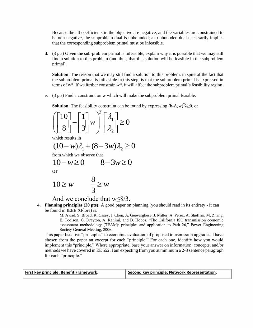
Because the all coefficients in the objective are negative, and the variables are constrained to

be non-negative, the subproblem dual is unbounded; an unbounded dual necessarily implies

that the corresponding subproblem primal must be infeasible.

d. (3 pts) Given the sub-problem primal is infeasible, explain why it is possible that we may still

find a solution to this problem (and thus, that this solution will be feasible in the subproblem

primal).

Solution: The reason that we may still find a solution to this problem, in spite of the fact that

the subproblem primal is infeasible in this step, is that the subproblem primal is expressed in

terms of w*. If we further constrain w*, it will affect the subproblem primal’s feasibility region.

e. (3 pts) Find a constraint on w which will make the subproblem primal feasible.

Solution: The feasibility constraint can be found by expressing (b-A2w)Tλ≥0, or

1

2

10 10

8 3

T

w

which results in

1 2(10 ) (8 3 ) 0w w

from which we observe that

10 0 8 3 0w w or

810

3w w

And we conclude that w≤8/3. 4. Planning principles (20 pts): A good paper on planning (you should read in its entirety - it can

be found in IEEE XPlore) is: M. Awad, S. Broad, K. Casey, J. Chen, A. Geevarghese, J. Miller, A. Perez, A. Sheffrin, M. Zhang,

E. Toolson, G. Drayton, A. Rahimi, and B. Hobbs, “The California ISO transmission economic

assessment methodology (TEAM): principles and application to Path 26,” Power Engineering

Society General Meeting, 2006.

This paper lists five “principles” to economic evaluation of proposed transmission upgrades. I have

chosen from the paper an excerpt for each “principle.” For each one, identify how you would

implement this “principle.” Where appropriate, base your answer on information, concepts, and/or

methods we have covered in EE 552. I am expecting from you at minimum a 2-3 sentence paragraph

for each “principle.”

First key principle: Benefit Framework: Second key principle: Network Representation:

Third key principle: Market Prices: Fourth key principle: Uncertainty:

Fifth key principle: Resource alternatives to

transmission expansion:

Fifth key principle (continued):

5. Transmission line parameters (16 pts): A 765 kV transmission line has phase separation of 36

feet. Each phase is a 4-conductor bundle with 24-inch diameter. The conductor type is Tern (795

kcmil). The following data is obtained from tables:

Ind reactance 1 ft spacing for 4-conductor bundle at 24’’: Xa=0.028Ω/mile

Ind reactance spacing factor for 36’ phase separation: Xd=0.4348Ω/mile

Cap reactance at 1ft spacing for 4 conductor bundle at 24’’: X’a=0.0051MΩ-mile

Cap reactance spacing factor for 36’ phase separation: X’d=0.1062MΩ-mile

a. (6 pts) Compute the SIL for this line configuration with 4 conductors per bundle.

Solution: Get per-unit length inductive reactance:

So XL=Xa+Xd=0.028+0.4348=0.4628 ohms/mile.

Now get per-unit length capacitive reactance.

XC=X’a+X’d=0.0051+0.1062=0.1113E6ohms-mile

So z=jXL=j0.4376 Ohms/mile, and

y=1/-jXC=1/-j(0.1113×106)=j8.9847×10-6 mhos/mile

226.96ohms 10×j8.9847

j.46286-

y

zZC

009+2.5785e

226.96

10765232

C

LLSIL

Z

VP

The SIL with 4 conductors is 2578 MW.

b. (4 pts) A designer considers reducing the number of conductors per bundle from 4 to 3, while

maintaining conductor spacing and phase spacing at 24 inches and 36 feet, respectively. Would

you expect this change to increase or decrease the surge impedance loading? Support your

answer.

Solution: The 3 conductor bundle is an equilateral triangle with a GMR of (r’*24*24)1/3,

whereas the 4 conductor bundle is a square with a GMR of (r’*24*24*33.94)1//4 where

33.94=sqrt(242+242). Therefore, the GMR Rb of the 3 conductor bundle is slightly smaller than

the GMR of the 4 conductor bundle. This causes the 3 conductor bundle to have larger inductive

and capacitive reactances, per the below equations,

/mile

dX

ln10022.2 1

ln10022.2 33

m

b

L Df

aX

RfX

mile-

'

ln10779.111

ln10779.11 66

d

X

Df

aX

RfX mc

b

C

and therefore a larger surge impedance and therefore a smaller SIL.

c. (6 pts) The designer desires to maximize the power transfer capability of the line. Relative to

the design of part (a)

If the line is 30 miles long, what changes would you consider?

Solution: Use a conductor with a larger diameter and therefore higher ampacity.

If the line is 300 miles long, what changes would you consider?

Solution: Increase SIL by decreasing phase spacing, increasing the number of

subconductors in a bundle, or increasing the bundle diameter.