1

Abstract—A novel fast electromagnetic field-circuit simulator

that permits the full-wave modeling of transients in nonlinear microwave circuits is proposed. This time-domain simulator is composed of two components: (i) A full-wave solver that models interactions of electromagnetic fields with conducting surfaces and finite dielectric volumes by solving time-domain surface and volume electric field integral equations, respectively; (ii) A circuit solver that models field interactions with lumped circuits, which are potentially active and nonlinear, by solving Kirchoff’s equations through modified nodal analysis. These field and circuit analysis components are consistently interfaced and the resulting coupled set of nonlinear equations is evolved in time by a multidimensional Newton-Raphson scheme. The solution procedure is accelerated by allocating field- and circuit-related computations across the processors of a distributed-memory cluster, which communicate using the message-passing interface standard. Furthermore, the electromagnetic field solver, whose demand for computational resources far outpaces that of the circuit solver, is accelerated by an FFT based algorithm, viz. the time-domain adaptive integral method. The resulting parallel FFT accelerated transient field-circuit simulator is applied to the analysis of various active and nonlinear microwave circuits, including power-combining arrays.

Index Terms—Parallel processing, microwave circuits, nonlinear circuits, time-domain integral equations, transient analysis.

I. INTRODUCTION S operating frequencies increase, accurate and efficient hybrid full-wave field-circuit simulation tools are

becoming increasingly indispensable in the design of microwave circuits as well as in the assessment of their vulnerability to unintentional coupling, crosstalk, packaging effects, and intentional electromagnetic interference. Microwave circuits can be analyzed using either frequency- or time-domain simulators; however, when the circuit under study contains nonlinear components, time-domain methods

Manuscript received September 22, 2004. This research was supported in

part by ARO program DAAD19-00-1-0464, by the DARPA VET Program under AFOSR contract F49620-01-1-0228, by the MURI grant F49620-01-1-04, "Analysis and design of ultra-wide band and high power microwave pulse interactions with electronic circuits and systems", and in part by the Computational Science and Engineering (CSE) fellowship at the University of Illinois at Urbana Champaign.

The authors are with the Center for Computational Electromagnetics, Department of Electrical and Computer Engineering, University of Illinois at Urbana-Champaign, Urbana, IL, 61801 USA (phone: 217-244-2636; fax: 217-333-5962; e-mail: ayilmaz@uiuc.edu).

enjoy the advantage of allowing for the direct analysis of field-circuit interactions without resorting to harmonic balance or port extraction methods [1]. Although early efforts at formulating hybrid time-domain field-circuit simulators relied on integral-equation schemes – the goal often consisted in the analysis of electromagnetic interactions with nonlinearly loaded wires [2]-[4] – most of the ensuing simulators invoked time-domain differential-equation methods. By now, various extensions to both the finite-difference time-domain (FDTD) [5]-[11] and finite-element time-domain (FETD) [12], [13] methods aimed at incorporating device physics/behavior into electromagnetic analysis environments have been proposed. The most rigorous of these schemes permit the simultaneous solution of the Maxwell and semiconductor carrier transport equations by casting them as a strongly coupled nonlinear system of differential equations on the same grid [14], [15]. To minimize computational cost, whenever possible, these differential equation solvers account for device and circuit behavior (as opposed to physics) through their description in terms of equivalent lumped elements and macromodels [16]. However, lumped loads and circuits, be they passive or active, linear or nonlinear, static or time-varying, can be quite easily accounted for in time-domain integral-equation solvers as well [1]-[4].

Indeed, the recent development of stable [17]-[19], accurate [20], and fast [21]-[29] marching on in time based integral-equation solvers for analyzing large-scale transient scattering and radiation phenomena calls for a study into the applicability of these solvers to the analysis of microwave circuits. Modern-day fast time-domain integral-equation solvers are either accelerated by plane wave time domain (PWTD) [22] or by fast Fourier transform (FFT) [23]-[29] based algorithms. Use of either algorithm permits the analysis of transient electromagnetic phenomena with far more degrees of freedom than possible by classical time-domain integral-equation approaches. Recently, a PWTD accelerated electromagnetic field solver was coupled to a SPICE-like circuit simulator and applied to the analysis of transients on microwave circuits with nonlinear loads [30]. Here, we report, instead, on the hybridization (formulation and implementation) of an FFT accelerated solver with a modified nodal analysis based circuit simulator; an initial implementation of this scheme was described in [31]. The main reason for pursuing FFT accelerated field-circuit analysis tools is as follows. Just like their frequency-domain

A Parallel FFT Accelerated Transient Field-Circuit Simulator Ali E. Yılmaz, Jian-Ming Jin, and Eric Michielssen

A

2

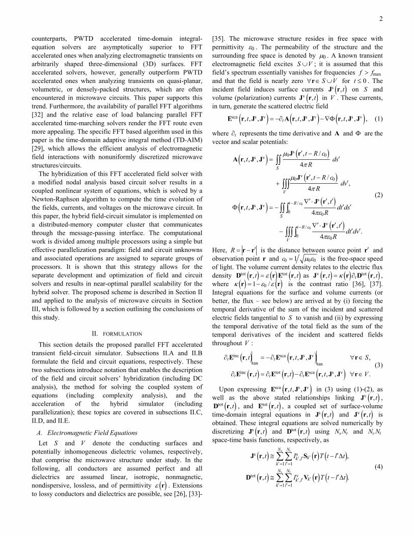
counterparts, PWTD accelerated time-domain integral-equation solvers are asymptotically superior to FFT accelerated ones when analyzing electromagnetic transients on arbitrarily shaped three-dimensional (3D) surfaces. FFT accelerated solvers, however, generally outperform PWTD accelerated ones when analyzing transients on quasi-planar, volumetric, or densely-packed structures, which are often encountered in microwave circuits. This paper supports this trend. Furthermore, the availability of parallel FFT algorithms [32] and the relative ease of load balancing parallel FFT accelerated time-marching solvers render the FFT route even more appealing. The specific FFT based algorithm used in this paper is the time-domain adaptive integral method (TD-AIM) [29], which allows the efficient analysis of electromagnetic field interactions with nonuniformly discretized microwave structures/circuits.

The hybridization of this FFT accelerated field solver with a modified nodal analysis based circuit solver results in a coupled nonlinear system of equations, which is solved by a Newton-Raphson algorithm to compute the time evolution of the fields, currents, and voltages on the microwave circuit. In this paper, the hybrid field-circuit simulator is implemented on a distributed-memory computer cluster that communicates through the message-passing interface. The computational work is divided among multiple processors using a simple but effective parallelization paradigm: field and circuit unknowns and associated operations are assigned to separate groups of processors. It is shown that this strategy allows for the separate development and optimization of field and circuit solvers and results in near-optimal parallel scalability for the hybrid solver. The proposed scheme is described in Section II and applied to the analysis of microwave circuits in Section III, which is followed by a section outlining the conclusions of this study.

II. FORMULATION This section details the proposed parallel FFT accelerated

transient field-circuit simulator. Subsections II.A and II.B formulate the field and circuit equations, respectively. These two subsections introduce notation that enables the description of the field and circuit solvers’ hybridization (including DC analysis), the method for solving the coupled system of equations (including complexity analysis), and the acceleration of the hybrid simulator (including parallelization); these topics are covered in subsections II.C, II.D, and II.E.

A. Electromagnetic Field Equations Let S and V denote the conducting surfaces and

potentially inhomogeneous dielectric volumes, respectively, that comprise the microwave structure under study. In the following, all conductors are assumed perfect and all dielectrics are assumed linear, isotropic, nonmagnetic, nondispersive, lossless, and of permittivity ( )ε r . Extensions to lossy conductors and dielectrics are possible, see [26], [33]-

[35]. The microwave structure resides in free space with permittivity 0ε . The permeability of the structure and the surrounding free space is denoted by 0µ . A known transient electromagnetic field excites S V∪ ; it is assumed that this field’s spectrum essentially vanishes for frequencies maxf f> and that the field is nearly zero S V∀ ∈ ∪r for 0t ≤ . The incident field induces surface currents ( )s , tJ r on S and volume (polarization) currents ( )v , tJ r in V . These currents, in turn, generate the scattered electric field

( ) ( ) ( )sca s v s v s v, , , , , , , , , ,tt t t= −∂ − ∇ΦE r J J A r J J r J J (1)

where t∂ represents the time derivative and A and Φ are the vector and scalar potentials:

( ) ( )

( )

( ) ( )

( )

0

0

s0 0s v

v0 0

s/s v

0 0

v/

0 0

, /, , ,

4

, / ,

4

,, , ,

4

, .

4

S

V

t R c

S

t R c

V

t R ct ds

R

t R cdv

R

tt dt ds

R

tdt dv

R

µ

π

µ

π

πε

πε

−

−

′ −′=

′ −′+

′ ′ ′∇ ⋅′ ′Φ = −

′ ′ ′∇ ⋅′ ′−

∫∫

∫∫∫

∫∫ ∫

∫∫∫ ∫

J rA r J J

J r

J rr J J

J r

(2)

Here, R ′= −r r is the distance between source point ′r and observation point r and 0 0 01c µ ε= is the free-space speed of light. The volume current density relates to the electric flux density ( ) ( ) ( )tot tot, ,t tε=D r r E r as ( ) ( ) ( )v tot, ,tt tκ= ∂J r r D r , where ( ) ( )01 /κ ε ε= −r r is the contrast ratio [36], [37]. Integral equations for the surface and volume currents (or better, the flux – see below) are arrived at by (i) forcing the temporal derivative of the sum of the incident and scattered electric fields tangential to S to vanish and (ii) by expressing the temporal derivative of the total field as the sum of the temporal derivatives of the incident and scattered fields throughout V :

( ) ( )

( ) ( ) ( )

inc sca s vtan tan

inc tot sca s v

, , , , ,

, , , , , .

t t

t t t

t t S

t t t V

∂ = −∂ ∀ ∈

∂ = ∂ − ∂ ∀ ∈

E r E r J J r

E r E r E r J J r (3)

Upon expressing ( )sca s v, , ,tE r J J in (3) using (1)-(2), as well as the above stated relationships linking ( )v , tJ r ,

( )tot , tD r , and ( )tot , tE r , a coupled set of surface-volume time-domain integral equations in ( )s , tJ r and ( )v , tJ r is obtained. These integral equations are solved numerically by discretizing ( )s , tJ r and ( )tot , tD r using s tN N and v tN N space-time basis functions, respectively, as

( ) ( ) ( )

( ) ( ) ( )

s s,

1 1

tot v,

1 1

, ,

, .

s t

v t

N N

kk lk lN N

kk lk l

t I T t l t

t I T t l t

′′ ′′ ′= =

′′ ′′ ′= =

′≅ − ∆

′≅ − ∆

∑ ∑

∑ ∑

J r S r

D r V r (4)

3

Here, s,k lI ′ ′ and v

,k lI ′ ′ are unknown expansion coefficients

(electromagnetic unknowns) and max/t fβ∆ = is the time-step size; typically 0.04 0.1β≤ ≤ . In this paper, the surface basis

functions ( )k ′S r are Rao-Wilton-Glisson (RWG) functions

[38] defined on pairs of triangular patches that approximate S . The volume basis functions ( )k ′V r are zeroth-order

divergence conforming functions [36] defined over tetrahedral elements, which approximate the dielectric volumes V , and over each of which ( )ε r (hence ( )κ r ) is assumed constant;

this implies that ( ) ( ) ( ) ( )v v,

1 1,

v tN N

k k tk lk l

t I T t l tκ ′ ′′ ′′ ′= =

′≅ ∂ − ∆∑ ∑J r r V r .

This choice of basis functions enforces the continuity of the normal component of the surface current density across patches and the electric flux density across tetrahedrons, respectively. The temporal basis functions ( )T t are shifted

Lagrange interpolants [18]. It is important to note that the composite basis functions in (4) are localized in space-time. Upon substituting (4) into (3) and testing the resulting equation at times l t∆ with the spatial functions

( ) ( )1 , , sNS r S r… and ( ) ( ) ( ) ( )1 1 , , ,v vN Nκ κr V r r V r… a total of

( )EM t s v tN N N N N= + equations for EM tN N expansion

coefficients result:

( )

EM EM

max 1,

for 1,2, , .g

l

l l tl ll l N

l N′− ′′= −

= =∑V Z I … (5)

Here, gN denotes the longest transit time of a free-space propagating electromagnetic field across S V∪ , expressed in terms of time steps [29]. Expressions for the entries of the vectors EM

lV and EMl′I and matrices l l′−Z are provided in the

Appendix. The system of equations (5) is recast into the following form and solved by forward substitution (i.e., by marching on in time):

( )

1EM EM EM

0max 1,

for 1,2, , .g

l

l l tl l ll l N

l N−

′− ′′= −

= − =∑Z I V Z I … (6)

The matrix 0Z , which represents immediate electromagnetic interactions, is a sparse but non-diagonal impedance matrix of size EM EMN N× , with typically ( )EMO N nonzero elements. The vectors EM

lI and EMlV hold the unknown current and flux

coefficients and the known tested incident field values at time l t∆ , respectively. The dominant computational cost of the field solver involves the evaluation of the space-time convolution appearing on the right-hand side of (6), viz. the computation of the scattered electromagnetic fields, which requires ( )2

EMO N operations per time step [29].

B. Circuit Equations The proposed solver allows the microwave structure

described above to contain an arbitrary number of lumped

circuits with independent reference/ground nodes. Equations governing circuit behaviors are formulated, starting from the circuit topologies and Kirchoff’s laws, via modified nodal analysis using the SPICE2 approach [39] as detailed next; specific details of how the circuits are coupled to the electromagnetic system are further discussed in subsection II.C. The circuit unknowns are node voltages and voltage-source currents; hence, the total number of circuit unknowns, denoted as CKTN , is equal to the total number of non-ground nodes and voltage sources in the circuits. A total of CKTN equations in terms of these unknowns are obtained by imposing Kirchoff’s voltage law at the voltage-defined elements and current law at all nodes except the grounds. Branch equations relating currents to voltages are obtained from element stamps and companion models that are formulated using the trapezoidal integration rule. The ciurcut unknowns are evolved in time using the same time step size as the field solver, t∆ , which is assumed constant throughout the simulation. While contemporary circuit solvers employ variable time stepping schemes, the fixed but small t∆ dictated by the field solver was found to be sufficiently accurate for the applications considered in this paper. When analyzing circuits composed of linear and nonlinear resistors, capacitors, inductors, as well as dependent and independent voltage and current sources for tN time steps, this procedure yields CKT tN N equations for CKT tN N unknowns:

( )CKT,nlCKT CKT CKT+ for 1, 2, , .tl l l l l N= =YV I V I … (7)

The matrix Y , which represents branch equations of linear and time-invariant circuit elements, is a sparse admittance matrix of size CKT CKTN N× with typically ( )CKTO N nonzero elements. The vectors CKT

lV and CKTlI hold the circuit

unknowns and source currents and voltages, respectively, and the vector ( )CKT,nl CKT

l lI V represents the branch equations of nonlinear and time-varying elements at time l t∆ .

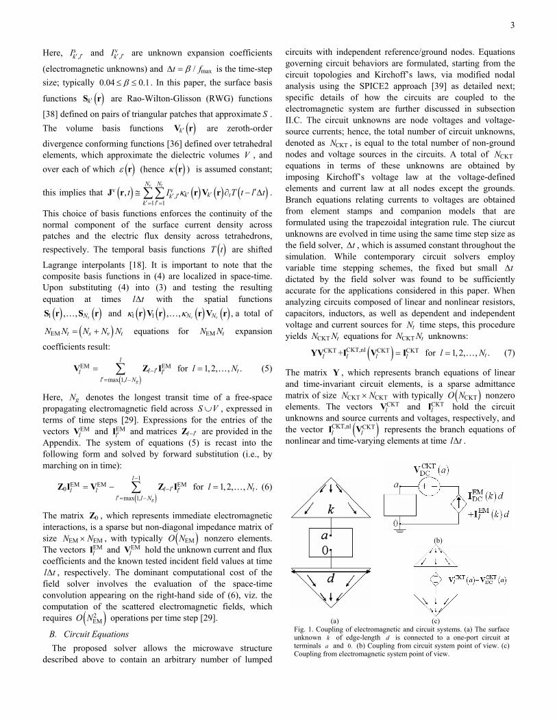
(b)

(a) (c) Fig. 1. Coupling of electromagnetic and circuit systems. (a) The surface unknown k of edge-length d is connected to a one-port circuit at terminals a and 0. (b) Coupling from circuit system point of view. (c) Coupling from electromagnetic system point of view.

4

C. Coupled System of Equations The lumped circuits are connected to the conducting

surfaces S through electromagnetic surface unknowns and are modeled as local voltage sources. To illustrate this procedure, assume that electromagnetic surface unknown k is loaded by a one-port circuit whose terminals are at nodes a and 0 (Fig. 1(a)). The field solver requires as one of its inputs the time-derivative of the voltage difference between the two terminals ( )CKT

t l a∂ V and the circuit solver requires the port current ( )EM

l k dI , where d is the length of the edge. Thus, the following coupled system of equations results when the two solvers are interfaced:

( ) ( )EMv

0CKT,nl CKTCKTi

1EM EM v

1CKT

= .

ll

l lll

l ll llll

l

−

′− ′′=

= +

− − =

∑

0IZ Cf x

I VVC Y

V Z I Kb

I

(8)

Here, EM CKT TT T

l l l = x I V is the vector of unknowns at

time l t∆ . The matrix iC , which represents field to circuit coupling, is formed according to Fig. 1(b) and is used to compute currents observed at the circuit terminals. The matrix

vC and the vector vlK , which represent circuit to field

coupling, are used to compute the numerical derivatives of terminal voltages and are formed according to Fig. 1(c). For circuits with three or more terminals, the entries of iC , vC , and v

lK can be found through a straightforward extension of the procedure in Fig. 1 [30]. In general, if there are PORTN ports, iC and vC will have a total of PORT2N nonzero elements. Other coupling schemes that introduce additional unknowns at the circuit terminals (contacts) exist [40]. Regardless of the scheme used, however, the off-diagonal matrix blocks representing coupling between the circuit and field formulations/solvers are sparse.

Notice that, while the circuit solver can incorporate initial conditions (typically computed from a DC analysis) for the circuit unknowns (i.e., CKT CKT

DC l= ≠V V 0 and CKT CKTDC l= ≠I I 0 for 0l = ), the field solver assumes zero

initial conditions (i.e., EMl =I 0 and EM

l =V 0 for 0l ≤ ). In this paper, microwave circuits with DC sources are analyzed in two ways: (i) Zero initial conditions are assumed everywhere; the DC sources are turned on gradually (in order not to violate the finite bandwidth assumption), and the transient analysis is performed only after the system reaches steady state. Depending on the specifics of the simulation being conducted, this procedure may require (too) many time steps and lead to low-frequency stability problems, which are avoided by the second scheme. (ii) The DC and transient responses are separated, similar to [10], [11], using the linearity of the electromagnetic system as follows. On the one hand, the total electromagnetic response at time l t∆ is represented as EM EM

DC l+I I and the field solver models only the transient response EM

lI . On the other hand, the total circuit response at time l t∆ is represented as CKT

lV and the circuit

solver models both the DC response and the transient response (by enforcing the DC solution as initial conditions through

CKTDCV and CKT

DCI ). To maintain consistency, DC voltages and currents are introduced at the interface (Fig. 1(b)). Hence, the hybrid field-circuit solver uses the (pre-computed) vectors

CKTDCV , CKT

DCI , and the entries of EMDCI at the circuit ports to

account for the DC conditions in the second scheme. These values can be computed through a DC analysis of the circuits with the microwave structure characterized either explicitly, e.g., through fast electrostatic solvers [41], or approximately, e.g., as a small resistor modeling the DC resistance of the conductors between circuits [11].

D. Solution Algorithm/Computational Complexity Analysis At each time step 1, 2, , tl N= … , the following five-stage

Newton-Raphson algorithm is used to solve the coupled nonlinear system of equations (8): Stage (i): Compute the right-hand-side vector lb . Then for each Newton iteration 1,2,p = …

Stage (ii): Evaluate the residual vector ( ), 1 , 1 ,l p l p l− −= −r f x b

where EM CKT, 1 , 1 , 1

TT Tl p l p l p− − −

= I Vx is the solution vector from

the previous Newton step and the initial guess is ,0 1l l−=x x , i.e., the solution at the previous time step. Stage (iii): If , 1l p ltol− < ×r b then stop; the solution at time

l t∆ is , 1l l p−=x x .

Stage(iv): Compute the Jacobian sub-matrix nl,l p =J

CKT, 1

CKT,nl

CKT .l p

l

l−

∂∂ V

IV

Stage (v): Iteratively solve

v

0, , 1i nl

,

l p p p l p

l p−

= = +

Z CJ s s r

C Y J (9)

for the Newton step ps and find the next solution vector , , 1l p l p p−= −x x s . Note that, in general all four submatrices of the Jacobian

matrix ,l pJ in (9) are sparse and the algorithm needs only one Newton iteration per time step if there are no nonlinear circuit elements. It should be emphasized that the above solution algorithm is different from that of [30]. While the algorithm in [30] solves a smaller system of equations and therefore might potentially require fewer Newton iterations, here the Jacobian matrix is computed significantly faster. This is because, unlike [30], the above algorithm does not require a matrix solution to compute the entries of ,l pJ ; indeed they can be computed analytically. Furthermore, the algorithm here is more amenable to the parallelization framework discussed in subsection II.E. The computational complexity of the above algorithm is analyzed next.

The algorithm evaluates and stores lb , which is independent of the Newton iteration, in ( )2

CKTEMO N N+ operations. Then, at each Newton iteration p , the algorithm

5

requires ( )EM CKTO N N+ operations to evaluate the vectors ( ), 1l p−f x and , 1l p−r , ( )nzO N operations to update nl

,l pJ , and ( )( )I EM CKTO N N N+ operations to solve for the Newton step.

Here, nzN is the number of nonzero entries of nl,l pJ and IN is

the average number of iterations needed to solve (9). In general, EM CKTN N and EM nzN N . Thus, the (two) dominant computational operations are the evaluation of the scattered electromagnetic fields in stage (i) and the iterative solution of the Newton step ps in stage (v). For each time step, the computations involved in stages (i) and (v) require

( )2CKTEMO N N+ and ( )( )P I EM CKTO N N N N+ operations,

respectively, where PN denotes the average number of Newton iterations. In our experience, the dominant computational operation for typical microwave circuits is incurred in stage (i), the calculation of lb .

E. Parallelization and TD-AIM Acceleration The solution of (8) is accelerated by parallel processing.

One parallelization approach might be to simultaneously distribute all EM CKTN N+ unknowns among the P available processors without separating electromagnetic and circuit unknowns. This approach, however, forces all processors handling both types of unknowns to run both electromagnetic and circuit solvers; this, in turn, leads to load balancing problems. Furthermore, it is not clear how to retrofit existing parallel field and circuit solvers to operate in unison inside such a framework. In this work, the parallelization strategy is to distribute electromagnetic- and circuit-related unknowns and operations to separate sets of processors. Of the

EM CKTP P+ available processors, EMP processors are dedicated to computations governing the updates of the EMN field unknowns and CKTP processors are used for operations related to updating the CKTN circuit unknowns. The two sets of processors communicate only when evaluating , 1l p−r and its norm and while iteratively solving (9) in the Newton-Raphson algorithm of subsection II.D. Moreover, the two systems interact only at the loading ports and hence the two sets of processors exchange only PORT2N numbers when they communicate. Thus, the total amount of communication between the two sets of processors is ( )P I PORTO N N N bytes at each time step and is negligible compared to other communication and computation costs. This strategy allows for the separate development of field and circuit solvers and enables hybridization of already developed and optimized parallel field and circuit solvers in the Newton-Raphson framework without loss of their load-balancing features. Indeed, in this paper the circuit solver is hybridized with a highly scalable parallel FFT based field solver [29] as described next.

The FFT-acceleration is employed to reduce the ( )2EMO N

cost of computing the first EMN entries of lb at each time step, which quickly overwhelms the EMP processors. FFT based algorithms for accelerating electromagnetic analysis originated with the k-space method [42], [43] and were initially used for frequency-domain analysis involving

uniformly discretized structures. They were later extended to incorporate nonuniformly discretized structures through the introduction of auxiliary uniform grids [41], [44] and parallelized [44]-[46] to allow large-scale static and time-harmonic analysis. Recently, FFT based algorithms have been adopted to permit the parallel analysis of electromagnetic transients on large arbitrarily shaped structures [23]-[29]. Here, the TD-AIM algorithm [29] is used.

The TD-AIM scheme embeds the microwave structure in an auxiliary 3D Cartesian grid with c cx cy czN N N N= × × nodes

that are separated by , ,x ys s∆ ∆ and zs∆ in the three orthogonal directions. Each of the impedance matrices is approximated as near FFT

l l l l l l′− ′ ′− −≈ +Z Z Z by using these auxiliary

grid points. The matrices nearl l′−Z help preserve accuracy by

reproducing the original entries of l l′−Z : their entries are nonzero for only near-field interactions, for which they are equal to FFT

l l l l′− ′−−Z Z . The matrices FFTl l′−Z , on the other hand,

are approximations of the original matrices that are efficiently multiplied with the vectors EM

l′I using multidimensional FFTs.

The TD-AIM algorithm computes the first EMN entries of lb in four steps: (I) At each time step l , all current-coefficients

EM1l−I are locally projected onto the auxiliary grid, such that

sources that reside on the auxiliary grid accurately approximate the transient fields radiated by the original sources outside a near-field region. In order to use only one auxiliary grid and the same propagation operators for both, the projection step for surface and volume sources is not identical. Because the fields radiated by volume sources require an additional temporal derivative (see (12) in Appendix), a finite difference scheme is used to compute the numerical derivatives of the volume coefficients, which are then projected on to the auxiliary grid. (II) Present and future transient fields produced by the sources on the auxiliary grid are computed on the same grid using vector- and scalar-potential propagators as described in [29] in a multilevel approach via global space-time FFTs. (III) The fields at time step l are locally interpolated from the vector- and scalar-potential values on the auxiliary grid onto the primary mesh. (IV) The errors in the near-field region are corrected by

computing ( )

1near EM

max 1, g

l

l l ll l N

−

′ ′−′= −

∑ Z I and adding it to the fields

computed via steps (I)-(III). In this paper, the projection and interpolation operators of steps (I) and (III) are found by matching the multipole moments of point sources on the auxiliary grid to those of x , y , and z components and the gradients of the functions ( )kS r and ( ) ( )kκ r V r [29], [44]. Hence, four projection matrices are used for surface and volume basis functions. Because the projection operations and the correction matrices near

l l′−Z are localized in space and time, the dominant computational burden of the TD-AIM scheme is

6

the computation of 4D space-time FFTs in step (II). Using a multilevel algorithm and employing parallel FFTs (e.g., via the FFTW library [32]), the space-time FFTs are computed in

( )( )2EMlog logc c gO N N N P+ operations per processor per

time step. A detailed description of the parallel FFTs in this context is given in [29]. For volumetric or quasi-planar structures EMcN N∼ , whereas 1/3

EMgN N∼ (for volumetric) or 1/2EMgN N∼ (for quasi-planar) [29].

To sum up, the two computationally dominant stages of the proposed algorithm, stages (i) and (v), are both accelerated by parallelization while stage (i) is further accelerated by the TD-AIM algorithm. For typical microwave circuits, neglecting the communication costs, the time spent in stages (i) and (v) at each time step scales as ( )2

EM EM EM CKT CKTlogO N N P N P+ and ( )( )P I EM EM CKT CKTO N N N P N P+ per processor, respectively. Ignoring the circuit processors and operations, the processors exchange, at each time step, a total of ( )EMO N bytes while computing FFTs in stage (i) and depending on the numbering and distribution of the unknowns amongst them

( )P IO N N to ( )P I EMO N N N bytes in stage (v). Hence, communication costs, which are subdominant to computation costs for stage (i), may become the bottleneck for stage (v) as the number of processors is increased.

III. APPLICATIONS The accuracy and efficiency of the proposed scheme are

demonstrated by analyzing various microwave systems and circuits. First an active antenna and a microwave amplifier are analyzed and the results obtained are compared to measurement and simulation data available in the literature. Next a grid amplifier is simulated and the results compared with both frequency-domain simulations and measurements available in the literature. In all simulations, the TD-AIM kernel matches up to third-order moments when projecting sources onto the auxiliary grid, and defines the near-field region of a basis function as the space extending 4 (auxiliary grid) cells in each direction away from it (that is, γ as defined in [29], is 4). Bandwidths of Gaussian pulses are specified as two-sided and quantify the frequency range over which spectral power densities are no less than 45 dB below their peak values. The results in this section are obtained using a cluster of 1 GHz Pentium III processors with CKT 1P = . In each and every case, the parallel efficiency of the scheme is examined by observing its run time and memory requirements. While a direct performance comparison with other simulators is not performed, the below applications clearly demonstrate the viability of the solver for analyzing large and detailed microwave systems and circuits.

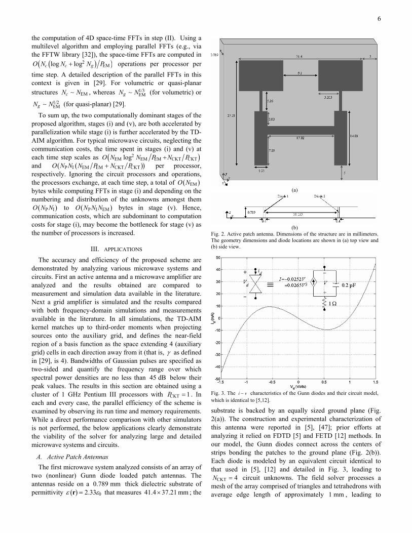
A. Active Patch Antennas The first microwave system analyzed consists of an array of

two (nonlinear) Gunn diode loaded patch antennas. The antennas reside on a 0.789 mm thick dielectric substrate of permittivity ( ) 02.33ε ε=r that measures 41.4 37.21 mm× ; the

substrate is backed by an equally sized ground plane (Fig. 2(a)). The construction and experimental characterization of this antenna were reported in [5], [47]; prior efforts at analyzing it relied on FDTD [5] and FETD [12] methods. In our model, the Gunn diodes connect across the centers of strips bonding the patches to the ground plane (Fig. 2(b)). Each diode is modeled by an equivalent circuit identical to that used in [5], [12] and detailed in Fig. 3, leading to

CKT 4N = circuit unknowns. The field solver processes a mesh of the array comprised of triangles and tetrahedrons with average edge length of approximately 1 mm , leading to

(a)

(b)

Fig. 2. Active patch antenna. Dimensions of the structure are in millimeters. The geometry dimensions and diode locations are shown in (a) top view and (b) side view.

Fig. 3. The i v− characteristics of the Gunn diodes and their circuit model, which is identical to [5,12].

7

6, 222sN = surface and 24,947vN = volume unknowns. The analysis is carried out for 1,000tN = time steps, with

5 pst∆ = and 40gN = . The TD-AIM accelerator uses an auxiliary grid with spacings 1 mmxs∆ = , 0.9 mmys∆ = , and

0.2 mmzs∆ = , resulting in 45 45 8cN = × × auxiliary grid points.

The array is excited by a normally incident x -polarized Gaussian plane wave pulse, with 0.1 mV/m peak-amplitude, 8 GHz center frequency, and 8 GHz bandwidth. The oscillations due to this low-power broadband plane wave are allowed to build up (Fig. 4(a)) and the resulting steady-state voltages across the diodes are plotted in Fig. 4(b). The oscillations across the two diodes are out of phase, as was observed in [5,12]. The fundamental frequency of the oscillations computed by the simulator is 12 GHz (Fig. 4(c)), which agrees well with the values of 12.2 GHz and 12.08 GHz computed via differential-equation based schemes of [5,12] and the measured value of 11.8 GHz . Figure 4(e) compares

the normalized y polarized electric-field pattern of the antenna in the x z− (H-) plane computed by the proposed method at 12 GHz to measurements at 11.8 GHz [47]. Good agreement is observed.

B. Microwave Amplifier To further verify the accuracy of the simulator, a nonlinear

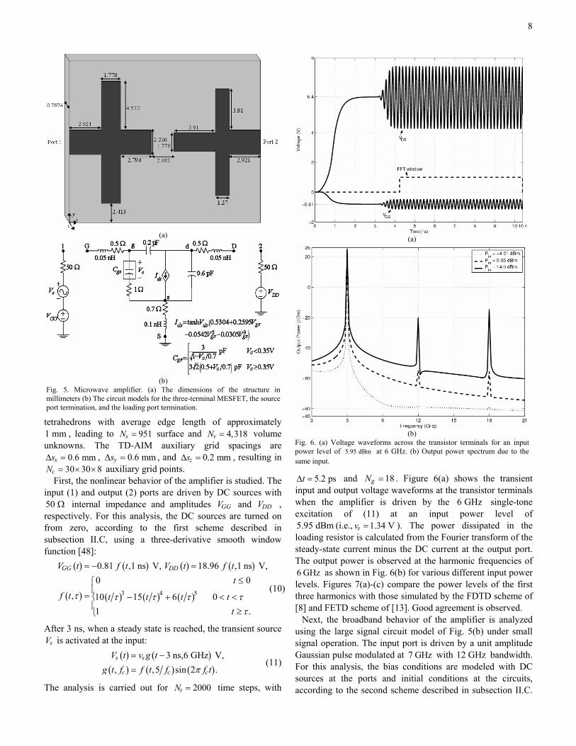
microwave amplifier circuit is analyzed next. Microstrip matching networks are connected to a packaged transistor, which resides on a 0.7874 mm thick dielectric substrate of permittivity ( ) 02.33ε ε=r that measures 17.526 16.256 mm;× the substrate is backed by an equally sized ground plane (Fig. 5(a)). This circuit was previously analyzed by FDTD based [8], FETD based [13], and PWTD accelerated integral-equation based [30] methods. Here, the circuit solver models the MESFET using the nonlinear large signal circuit model in Fig. 5(b), which is similar to those in [8], [13], [30]; a total of

CKT 9N = circuit unknowns result. The field solver processes a mesh of the microwave amplifier comprised of triangles and

(a) (b)

(c) (d) Fig. 4. (a) Transient voltage on the first diode. (b) Steady stage voltages across the diodes. (c) Frequency spectrum of the voltage across diode 1. (d) Radiation pattern of the active patch antenna at 12.0 GHz compared to measured values at 11.8 GHz.

8

tetrahedrons with average edge length of approximately 1 mm , leading to 951sN = surface and 4,318vN = volume unknowns. The TD-AIM auxiliary grid spacings are

0.6 mmxs∆ = , 0.6 mmys∆ = , and 0.2 mmzs∆ = , resulting in 30 30 8cN = × × auxiliary grid points.

First, the nonlinear behavior of the amplifier is studied. The input (1) and output (2) ports are driven by DC sources with 50 Ω internal impedance and amplitudes GGV and DDV , respectively. For this analysis, the DC sources are turned on from zero, according to the first scheme described in subsection II.C, using a three-derivative smooth window function [48]:

( ) ( ) ( ) ( )

( ) ( ) ( ) ( )3 4 5

0.81 ,1 ns V, 18.96 ,1 ns V,0 0

, 10 15 6 01 .

GG DDV t f t V t f tt

f t t t t tt

τ τ τ τ ττ

= − =

≤= − + < < ≥

(10)

After 3 ns, when a steady state is reached, the transient source sV is activated at the input:

( ) ( )

( ) ( ) ( )3 ns,6 GHz V,

, ,5 sin 2 .s s

c c c

V t v g tg t f f t f f tπ

= −

= (11)

The analysis is carried out for 2000tN = time steps, with

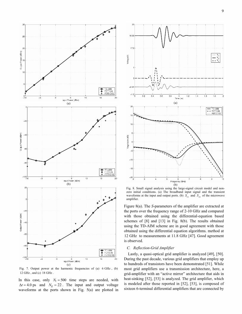
5.2 pst∆ = and 18gN = . Figure 6(a) shows the transient input and output voltage waveforms at the transistor terminals when the amplifier is driven by the 6 GHz single-tone excitation of (11) at an input power level of 5.95 dBm (i.e., 1.34 Vsv = ). The power dissipated in the loading resistor is calculated from the Fourier transform of the steady-state current minus the DC current at the output port. The output power is observed at the harmonic frequencies of 6 GHz as shown in Fig. 6(b) for various different input power levels. Figures 7(a)-(c) compare the power levels of the first three harmonics with those simulated by the FDTD scheme of [8] and FETD scheme of [13]. Good agreement is observed.

Next, the broadband behavior of the amplifier is analyzed using the large signal circuit model of Fig. 5(b) under small signal operation. The input port is driven by a unit amplitude Gaussian pulse modulated at 7 GHz with 12 GHz bandwidth. For this analysis, the bias conditions are modeled with DC sources at the ports and initial conditions at the circuits, according to the second scheme described in subsection II.C.

(a)

(b) Fig. 6. (a) Voltage waveforms across the transistor terminals for an input power level of 5.95 dBm at 6 GHz. (b) Output power spectrum due to the same input.

(a)

(b) Fig. 5. Microwave amplifier. (a) The dimensions of the structure in millimeters (b) The circuit models for the three-terminal MESFET, the source port termination, and the loading port termination.

9

In this case, only 500tN = time steps are needed, with 4.0 pst∆ = and 22gN = . The input and output voltage

waveforms at the ports shown in Fig. 5(a) are plotted in

Figure 8(a). The S-parameters of the amplifier are extracted at the ports over the frequency range of 2-10 GHz and compared with those obtained using the differential-equation based schemes of [8] and [13] in Fig. 8(b). The results obtained using the TD-AIM scheme are in good agreement with those obtained using the differential equation algorithms. method at 12 GHz to measurements at 11.8 GHz [47]. Good agreement is observed.

C. Reflection-Grid Amplifier Lastly, a quasi-optical grid amplifier is analyzed [49], [50].

During the past decade, various grid amplifiers that employ up to hundreds of transistors have been demonstrated [51]. While most grid amplifiers use a transmission architecture, here, a grid-amplifier with an “active mirror” architecture that aids in heat-sinking [52], [53] is analyzed. The grid amplifier, which is modeled after those reported in [52], [53], is composed of sixteen 6-terminal differential amplifiers that are connected by

(a)

(b) Fig. 8. Small signal analysis using the large-signal circuit model and non-zero initial conditions. (a) The broadband input signal and the transient waveforms at the input and output ports. (b) 11S and 21S of the microwave amplifier.

(a)

(b)

(c) Fig. 7. Output power at the harmonic frequencies of (a) 6 GHz , (b) 12 GHz , and (c) 18 GHz .

10

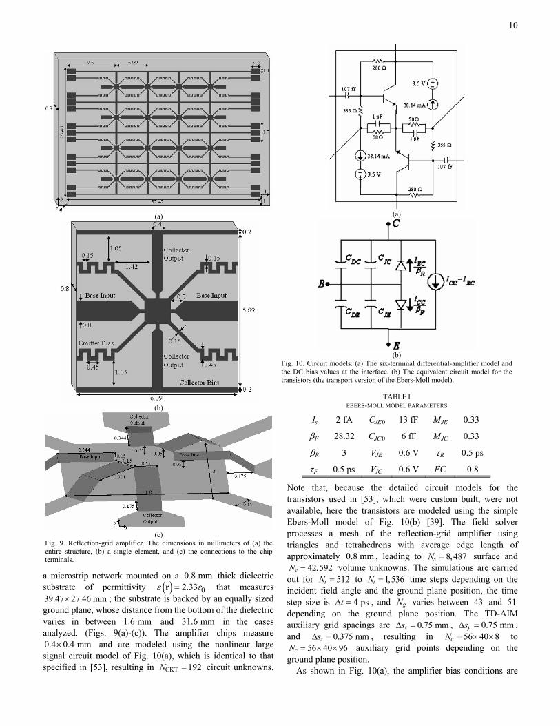
a microstrip network mounted on a 0.8 mm thick dielectric substrate of permittivity ( ) 02.33ε ε=r that measures 39.47 27.46 mm× ; the substrate is backed by an equally sized ground plane, whose distance from the bottom of the dielectric varies in between 1.6 mm and 31.6 mm in the cases analyzed. (Figs. 9(a)-(c)). The amplifier chips measure 0.4 0.4 mm× and are modeled using the nonlinear large signal circuit model of Fig. 10(a), which is identical to that specified in [53], resulting in CKT 192N = circuit unknowns.

Note that, because the detailed circuit models for the transistors used in [53], which were custom built, were not available, here the transistors are modeled using the simple Ebers-Moll model of Fig. 10(b) [39]. The field solver processes a mesh of the reflection-grid amplifier using triangles and tetrahedrons with average edge length of approximately 0.8 mm , leading to 8,487sN = surface and

42,592vN = volume unknowns. The simulations are carried out for 512tN = to 1,536tN = time steps depending on the incident field angle and the ground plane position, the time step size is 4 pst∆ = , and gN varies between 43 and 51 depending on the ground plane position. The TD-AIM auxiliary grid spacings are 0.75 mmxs∆ = , 0.75 mmys∆ = , and 0.375 mmzs∆ = , resulting in 56 40 8cN = × × to

56 40 96cN = × × auxiliary grid points depending on the ground plane position.

As shown in Fig. 10(a), the amplifier bias conditions are

(a)

(b)

(c) Fig. 9. Reflection-grid amplifier. The dimensions in millimeters of (a) the entire structure, (b) a single element, and (c) the connections to the chip terminals.

(a)

(b)

Fig. 10. Circuit models. (a) The six-terminal differential-amplifier model and the DC bias values at the interface. (b) The equivalent circuit model for the transistors (the transport version of the Ebers-Moll model).

TABLE I EBERS-MOLL MODEL PARAMETERS

sI 2 fA 0JEC 13 fF JEM 0.33

Fβ 28.32 0JCC 6 fF JCM 0.33

Rβ 3 JEV 0.6 V Rτ 0.5 ps

Fτ 0.5 ps JCV 0.6 V FC 0.8

11

modeled by DC sources at the ports. After the DC conditions at the circuits are established via the second scheme described in subsection II.C, the grid is illuminated by a ˆ ˆcos sinθ θ−x z polarized Gaussian plane wave, with 1 V/m peak-amplitude, 10 GHz center frequency, and 10 GHz bandwidth. In the following simulations, the plane wave is incident from the

ˆ ˆsin cosθ θ+x z direction and the gain of the grid is defined as the y (cross) polarized radar cross section of the structure at the specular angle ( ˆ ˆsin cosθ θ− +x z direction) divided by the top-surface area of the grid ( 237.47 25.46 mm× ); this replicates the gain definitions of the measurement setup in [51-53]. First, for verification purposes, the gain of the grid under normal illumination computed by the proposed scheme is compared to that computed by a frequency-domain hybrid simulator. The frequency-domain simulator’s circuit-solver replaces the transistors with their small-signal models at the operating point, whereas its field-solver uses a (frequency-domain) AIM accelerated integral-equation scheme [43],

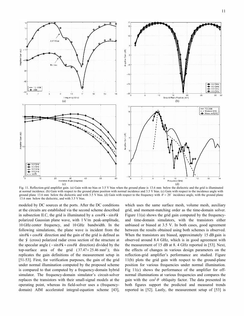
which uses the same surface mesh, volume mesh, auxiliary grid, and moment-matching order as the time-domain solver. Figure 11(a) shows the grid gain computed by the frequency- and time-domain simulators, with the transistors either unbiased or biased at 3.5 V. In both cases, good agreement between the results obtained using both schemes is observed. When the transistors are biased, approximately 15 dB gain is observed around 8.4 GHz, which is in good agreement with the measurement of 15 dB at 8. 4 GHz reported in [53]. Next, the effects of changes in various design parameters on the reflection-grid amplifier’s performance are studied. Figure 11(b) plots the grid gain with respect to the ground-plane position for various frequencies under normal illumination. Fig 11(c) shows the performance of the amplifier for off-normal illuminations at various frequencies and compares the gain with the 2cos θ obliquity factor. The data presented in both figures support the predicted and measured trends reported in [52]. Lastly, the measurement setup of [53] is

(a) (b)

(c) (d) Fig. 11. Reflection-grid amplifier gain. (a) Gain with no bias or 3.5 V bias when the ground plane is 13.6 mm below the dielectric and the grid is illuminated at normal incidence. (b) Gain with respect to the ground plane position with normal incidence and 3.5 V bias. (c) Gain with respect to the incidence angle with ground plane 13.6 mm below the dielectric and with 3.5 V bias. (d) Gain with respect to the frequency with 20θ = incidence angle, with the ground plane 13.6 mm below the dielectric, and with 3.5 V bias.

12

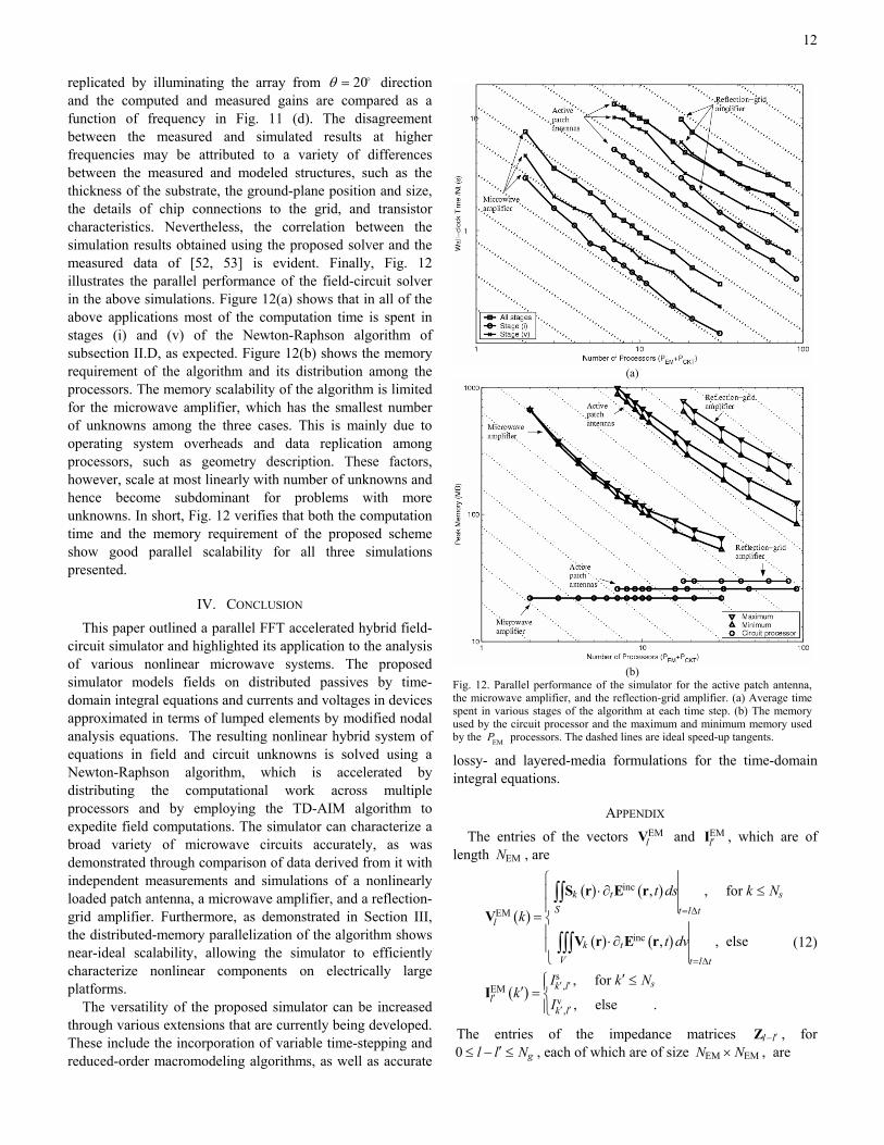
replicated by illuminating the array from 20θ = direction and the computed and measured gains are compared as a function of frequency in Fig. 11 (d). The disagreement between the measured and simulated results at higher frequencies may be attributed to a variety of differences between the measured and modeled structures, such as the thickness of the substrate, the ground-plane position and size, the details of chip connections to the grid, and transistor characteristics. Nevertheless, the correlation between the simulation results obtained using the proposed solver and the measured data of [52, 53] is evident. Finally, Fig. 12 illustrates the parallel performance of the field-circuit solver in the above simulations. Figure 12(a) shows that in all of the above applications most of the computation time is spent in stages (i) and (v) of the Newton-Raphson algorithm of subsection II.D, as expected. Figure 12(b) shows the memory requirement of the algorithm and its distribution among the processors. The memory scalability of the algorithm is limited for the microwave amplifier, which has the smallest number of unknowns among the three cases. This is mainly due to operating system overheads and data replication among processors, such as geometry description. These factors, however, scale at most linearly with number of unknowns and hence become subdominant for problems with more unknowns. In short, Fig. 12 verifies that both the computation time and the memory requirement of the proposed scheme show good parallel scalability for all three simulations presented.

IV. CONCLUSION This paper outlined a parallel FFT accelerated hybrid field-

circuit simulator and highlighted its application to the analysis of various nonlinear microwave systems. The proposed simulator models fields on distributed passives by time-domain integral equations and currents and voltages in devices approximated in terms of lumped elements by modified nodal analysis equations. The resulting nonlinear hybrid system of equations in field and circuit unknowns is solved using a Newton-Raphson algorithm, which is accelerated by distributing the computational work across multiple processors and by employing the TD-AIM algorithm to expedite field computations. The simulator can characterize a broad variety of microwave circuits accurately, as was demonstrated through comparison of data derived from it with independent measurements and simulations of a nonlinearly loaded patch antenna, a microwave amplifier, and a reflection-grid amplifier. Furthermore, as demonstrated in Section III, the distributed-memory parallelization of the algorithm shows near-ideal scalability, allowing the simulator to efficiently characterize nonlinear components on electrically large platforms.

The versatility of the proposed simulator can be increased through various extensions that are currently being developed. These include the incorporation of variable time-stepping and reduced-order macromodeling algorithms, as well as accurate

lossy- and layered-media formulations for the time-domain integral equations.

APPENDIX The entries of the vectors EM

lV and EMl′I , which are of

length EMN , are

( )

( ) ( )

( ) ( )

( )

inc

EM

inc

s,EM

v,

, , for

, , else

, for

, else .

k t sS t l t

l

k tV t l t

sk ll

k l

t ds k N

k

t dv

I k Nk

I

= ∆

= ∆

′ ′′

′ ′

⋅∂ ≤

=

⋅∂

′ ≤′ =

∫∫

∫∫∫

S r E r

V

V r E r

I

(12)

The entries of the impedance matrices l l′−Z , for 0 gl l N′≤ − ≤ , each of which are of size EM EMN N× , are

(a)

(b) Fig. 12. Parallel performance of the simulator for the active patch antenna, the microwave amplifier, and the reflection-grid amplifier. (a) Average time spent in various stages of the algorithm at each time step. (b) The memory used by the circuit processor and the maximum and minimum memory used by the EMP processors. The dashed lines are ideal speed-up tangents.

13

( )( )

( ) ( )( )

( )

( ) ( )( )

( ) ( )

( )( )

2 s

s

2 v

v

2 s

,( ) ,

( ) , for ,

( ) ,

( ) , for ,

( ) ,

( )

l l

k t kS

k t k s sS t l l t

k t kS

k t k s sS t l l t

k k t kV

k k t

k kt ds

t ds k N k N

t ds

t ds k N k N

t dv

φ

φ

κ

κ φ

′−

′

′

′= − ∆

′

′

′= − ∆

′

′

′

⋅∂

′+ ∇⋅ ∂ ≤ ≤

⋅∂

′+ ∇⋅ ∂ > ≤

=⋅∂

+ ∇⋅ ∂

∫∫

∫∫

∫∫

∫∫

∫∫∫

ZS r A r

S r r

S r A r

S r r

r V r A r

r V r ( )( )

( ) ( ) ( )( ) ( )

( )( ) ( )( )

s

2 v

v

, for ,

( ) ,

( ) , for , .

k s sV t l l t

t kk k t k

V

k k t k s sV t l l t

t dv k N k N

T tt dv

t dv k N k N

κε

κ φ

′= − ∆

′′

′

′= − ∆

′≤ > ∂ ⋅ +∂ ′+ ∇⋅ ∂ > >

∫∫∫

∫∫∫

∫∫∫

r

V rr V r A r

r

r V r r(13)

Notice that the first and second conditions in (3) are enforced on conductor surfaces and dielectric volumes by testing them with surface and volume functions, respectively. In (13), the entries of l l′−Z are defined in terms of the first and second time derivatives of scalar and vector potentials due to each spatial basis function, respectively:

( ) ( ) ( )

( ) ( ) ( )

( ) ( ) ( ) ( )

( ) ( ) ( ) ( )

0s

02

0 02 s

0v

03

0 02 v

/, ,

4/

, ,4/

, ,4

/, .

4

k

k

kt

S

t kt k

St k k

tV

t k kt k

V

T t R ct ds

RT t R c

t dsR

T t R ct dv

RT t R c

t dvR

φπε

µπ

κφ

πεµ κπ

′

′

′

′′

′ ′

′ ′′

′ ′− ∇ ⋅′∂ =

′∂ −′∂ =

′ ′ ′∂ − ∇ ⋅′∂ =

′ ′∂ −′∂ =

∫∫

∫∫

∫∫∫

∫∫∫

S rr

S rA r

r V rr

r V rA r

(14)

ACKNOWLEDGMENT We acknowledge the CSE department and the National

Center for Supercomputing Applications (NCSA) for access to their parallel clusters. A. E. Yılmaz thanks B. Fischer and Dr. K. Aygün for a reference circuit-solver program.

REFERENCES [1] E. K. Miller, “Time-domain modeling in electromagnetics,” J.

Electromagn. Waves Appl., vol. 8, no. 9/10, pp. 1125-1172, 1994. [2] H. Schuman, “Time-domain scattering from a nonlinearly loaded wire,”

IEEE Trans. Antennas Propagat., vol. 22, pp. 611-613, July 1974. [3] T. K. Liu and F. M. Tesche, “Analysis of antennas and scatterers with

nonlinear loads,” IEEE Trans. Antennas Propagat., vol. 24, no. 2, pp. 131-139, Mar. 1976.

[4] J. A. Landt, E. K. Miller, and F. J. Deadrick, “Time domain modeling of nonlinear loads,” IEEE Trans. Antennas Propagat., vol. 31, no. 1, pp. 121-126, Jan. 1983.

[5] B. Toland, J. Lin, B. Houshmand, and T. Itoh, “FDTD analysis of an active antenna,” IEEE Microwave Guided Wave Lett., vol. 3, no. 11, pp. 423-425, Nov. 1993.

[6] V. A. Thomas, M. E. Jones, M. Piket-May, A. Taflove, and E. Harrigan, “The use of SPICE lumped circuits as sub-grid models for FDTD analysis,” IEEE Microwave Guided Wave Lett., vol. 4, no. 5 pp. 141-143, May 1994.

[7] P. Ciampolini, P. Mezzanotte, L. Roselli, and R. Sorrentino, “Accurate and efficient circuit simulation with lumped-element FDTD technique,” IEEE Trans. Microwave Theory Tech., vol. 44, no. 12, pp. 2207-2215, Dec. 1996.

[8] C. Kuo, B. Houshmand, and T. Itoh, “Full-wave analysis of packaged microwave circuits with active and nonlinear devices: An FDTD approach,” IEEE Trans. Microwave Theory Tech., vol. 45, no. 5, pp. 819-826, May 1997.

[9] K.-P. Ma, B. Houshmand, Y. Qian, and T. Itoh, “Global time-domain full-wave analysis of microwave circuits involving highly nonlinear phenomena and EMC effects,” IEEE Trans. Microwave Theory Tech., vol. 47, no.6, pp. 859-866, June 1999.

[10] G. Kobidze, A. Nishizawa, and S. Tanabe, “Ground bouncing in PCB with integrated circuits,” IEEE Int. Symp. EMC, vol. 1, pp. 349-352, Aug.2000.

[11] N. Orhanovic, R. Raughuram, and N. Matsui, “Full wave analysis of planar interconnect structures using FDTD-SPICE,” IEEE Electronic Comp. Tech. Conf., pp. 489-494, 2001.

[12] K. Guillouard, M. F. Wong, V. F. Hanna, and J. Citerne, “A new global time-domain electromagnetic simulator of microwave circuits including lumped elements based on finite-element method,” IEEE Trans. Microwave Theory Tech., vol. 47, no. 10, pp. 2045-2048, Oct. 1999.

[13] S.-H. Chang, R. Coccioli, Y. Qian, and T. Itoh, “A global finite-element time-domain analysis of active nonlinear microwave circuits,” IEEE Trans. Microwave Theory Tech., vol. 47, pp. 2410-2416, Dec. 1999.

[14] M. A. Alsunaidi, S. M. S. Imtiaz, and S. M. El-Ghazaly, “Electromagnetic wave effects on microwave transistors using a full-wave time-domain model,” IEEE Trans. Microwave Theory Tech., vol. 44, pp. 799-808, June 1996.

[15] R. O. Grondin, S. M. El-Ghazaly, and S. Goodnick, “A review of global modeling of charge transport in semiconductors and full-wave electromagnetics,” IEEE Trans. Microwave Theory Tech., vol. 47, no. 6, pp. 817-829, June 1999.

[16] S. Grivet-Talocia, I. S. Stievano, and F. G. Canavero, “Hybridization of FDTD and device behavioral-modeling techniques,” IEEE Trans. Electromagn. Compat., vol. 45, no. 1, pp. 31-42, Feb. 2003.

[17] A. Sadigh and E. Arvas, “Treating the instabilities in marching-on-in-time method from a different perspective,” IEEE Trans. Antennas Propagat., vol. 41, no. 12, pp. 1695-1702, Dec. 1993.

[18] G. Manara, A. Monorchio, and R. Reggiannini, “A space-time discretization criterion for a stable time-marching solution of the electric field integral equation,” IEEE Trans. Antennas Propagat., vol. 45, pp. 527-532, Apr. 1997.

[19] J. Garret, A. E. Ruehli, and C. R. Paul, “Accuracy and stability improvements of integral equation models using the partial element equivalent circuit (PEEC) approach,” IEEE Trans. Antennas Propagat., vol. 46, no. 12, pp. 1824-1832, Dec. 1998.

[20] D. S. Weile, G. Pisharody, N.-W. Chen, B. Shanker, and E. Michielssen, “A novel scheme for the solution of time-domain integral equations of electromagnetics,” IEEE Trans. Antennas Propagat., vol. 52, pp. 283-295, 2004.

[21] S. P. Walker and C. Y. Leung, “Parallel computation of time-domain integral equation analyses of electromagnetic scattering and RCS,” IEEE Trans. Antennas Propagat., vol. 45, no. 4, Apr. 1997.

[22] B. Shanker, A. A. Ergin, M. Lu, and E. Michielssen, “Fast analysis of transient electromagnetic scattering phenomena using the multilevel plane wave time domain algorithm,” IEEE Trans. Antennas Propagat., vol. 51, no. 3, pp. 628-641, Mar. 2003.

[23] J. L. Hu, C. H. Chan, and Y. Xu, “A fast solution of time domain integral equation using fast Fourier transformation,” Microwave Opt. Tech.. Lett., vol. 25, no. 3, pp. 172-175, 2000.

[24] A. E. Yılmaz, D. S. Weile, J. M. Jin, and E. Michielssen, “A fast Fourier transform accelerated marching-on-in-time algorithm for electromagnetic analysis,” Electromagn., vol. 21, pp. 181-197, 2001.

[25] A. E. Yılmaz, D. S. Weile, J. M. Jin, and E. Michielssen, “A hierarchical FFT algorithm for fast analysis of transient electromagnetic scattering

14

phenomena,” IEEE Trans. Antennas Propagat., vol. 5, no. 7, pp. 971-982, July 2002.

[26] A. E. Yılmaz, D. S. Weile, B. Shanker, J. M. Jin, and E. Michielssen, “Fast analysis of transient scattering in lossy media,” IEEE Antennas Wireless Propagat. Lett., vol. 1, pp. 14-17, 2002.

[27] E. Bleszynski, M. Bleszynski, and T. Jaroszewicz, “A new fast time domain integral equation solution algorithm,” IEEE APS Symp. Digest, vol. 4, pp. 176-179, 2001.

[28] A. E. Yılmaz, K. Aygün, J. M. Jin, and E. Michielssen, “Matching criteria and the accuracy of time domain adaptive integral method,” IEEE APS Symp. Digest, vol. 2, pp. 166-169, 2002.

[29] A. E. Yılmaz, J. M. Jin, and E. Michielssen, “Time domain adaptive integral method for surface integral eqautions,” to appear in IEEE Trans. Antennas Propagat., Oct. 2004.

[30] K. Aygün, B. C. Fisher, J. Meng, and E. Michielssen, “A fast hybrid field-circuit simulator for transient analysis of microwave circuits,” IEEE Trans. Microwave Theory Tech., vol. 52, no. 2, pp. 573-583, Feb. 2004.

[31] A. E. Yılmaz, J. M. Jin, and E. Michielssen, “A parallel time-domain adapative integral method based hybrid field-circuit simulator,” IEEE APS Symp. Digest, vol. 3, pp. 3309-3312, 2004.

[32] M. Frigo and S. G. Johnson, “FFTW: An adaptive software architecture for the FFT,” Proc. IEEE ICASSP, vol. 3, pp. 1381-1384, 1998. Available: www.fftw.org.

[33] M. J. Bluck, S. P. Walker, and M. D. Pocock, “The extension of time-domain integral equation analysis to scattering from imperfectly conducting bodies,” IEEE Trans. Antennas Propagat., vol. 49, no. 6, pp. 875-879, June 2001.

[34] Q. Chen, M. Lu, and E. Michielssen, “Integral-equation-based analysis of transient scattering from surfaces with an impedance boundary condition,” Microwave Opt. Tech. Lett., vol. 42, no. 3, pp. 213-220, 2004.

[35] B. Shanker, K. Aygün, and E. Michielssen, “Fast analysis of transient scattering from lossy inhomogeneous dielectric bodies,” Radio Sci., vol. 39, no.2, pp. 1-14, 2004.

[36] D. H. Schaubert, D. R. Wilton, and A. W. Glisson, “A tetrahedral modeling method for electromagnetic scattering by arbitrarily shaped inhomogenous dielectric bodies,” IEEE Trans. Antennas Propagat., vol. 32, no. 1, pp. 77-85, Jan. 1984.

[37] N. T. Gres, A. A. Ergin, and E. Michielssen, “Volume-integral-equation-based analysis of transient electromagnetic scattering from three-dimensional inhomogeneous dielectric objects,” vol. 36, no. 3, Radio Sci., pp. 379-386, May/June 2001.

[38] S. M. Rao, D. R. Wilton, and A. W. Glisson, “Electromagnetic scattering by surfaces of arbitrary shape,” IEEE Trans. Antennas Propagat., vol. 30, no. 3, pp. 409-418, May 1982.

[39] A. Vladimirescu, The SPICE Book. New York: John Wiley & Sons, 1994.

[40] Y. Wang, D.Gope, V. Jandhyala, and C.-J. R. Shi, “Generalized Kirchoff’s current and voltage law formulation for coupled circuit-electromagnetic simulation with surface integral equations,” IEEE Trans. Microwave Theory Tech., vol. 52, pp. 1673-1682, Jul. 2004.

[41] J. R. Phillips and J. K. White, “A precorrected-FFT method for electrostatic analysis of complicated 3-D structures,” IEEE Trans. Computer-Aided Design of Integrated Circuits and Systems, vol. 16, no. 10, pp. 1059-1072, Oct. 1997.

[42] N. N. Bojarski, “K-space formulation of the electromagnetic scattering problem,” URSI Digest, p. 117, 1971.

[43] N. N. Bojarski, “The k-space formulation of the scattering problem in the time domain,” J. Acoust. Soc. Am., vol. 72, no. 2, pp. 570-584, Apr. 1982.

[44] E. Bleszynski, M. Bleszynski, and T. Jaroszewicz, “AIM: Adaptive integral method for solving large-scale electromagnetic scattering and radiation problems,” Radio Sci., vol. 31, no. 5, pp. 1125-1251, 1996.

[45] H. T. Anastassiu, M. Smelyanskiy, S. Bindiganavale, and J. L. Volakis, “Scattering from relatively flat surfaces using the adaptive integral method,” Radio Sci., vol. 33, no. 1, pp. 7-16, 1998.

[46] N. R. Aluru, V. B. Nadkarni, and J. White, “A parallel precorrected FFT based capacitance extraction program for signal integrity analysis,” Proc. of Design Automation Conf., pp. 363-366, 1996.

[47] B. Toland, J. Lin, B. Houshmand, and T. Itoh, “Electromagnetic simulation of mode control of a two element active antenna,” IEEE MTT-S Symp. Dig., pp. 883-886, 1994.

[48] R. W. Ziolkowski and E. Heyman, “Wave propagation in media having negative permittivity and permeability,” Phys. Rev. E., vol. 64, 056625, 2001.

[49] J. W. Mink, “Quasi-optical power combining of solid-state millimeter-wave sources,” IEEE Trans. Microwave Theory Tech., vol. 34, no. 2, pp. 273-279, Feb. 1986.

[50] R. M. Weikle II, M. Kim, J. B. Hacker, M. P. Delisio, Z. B. Popovic, D. Rutledge, “Transistor oscillator and amplifier grids,” Proc. IEEE, vol. 80, no. 11, pp. 1800-1809, Nov. 1992.

[51] M. P. Delisio, S. W. Duncan, D.-W. Tu, C-M. Liu, A. Moussessian, J. J. Rosenberg, and D. B. Rutledge, “Modeling and performance of a 100-element pHEMT grid amplifier,” IEEE Trans. Microwave Theory Tech., vol. 44, no. 12, pp. 2136-2144, Dec. 1996.

[52] F. Lecuyer, R. Swisher, I.-F. F. Chio, A. Guyette, A. Al-Zayed, W. Ding, M. Delisio, K. Sato, A. Oki, A. Gutierrez, R. Kagiwada, and J. Cowles, “A 16-element reflection grid amplifier,” IEEE MTT-S Symp. Dig., pp. 809-812, 2000.

[53] A. Guyette, R. Swisher, F. Lecuyer, A. Al-Zayed, A. Kom, S-T Lei, M. Oliviera, P. Li, M. Delisio, K. Sato, A. Oki, A. Gutierrez-Aitken, R. Kagiwada, and J. Cowles, “A 16-element reflection grid amplifier with improved heat sinking,” IEEE MTT-S Symp. Dig., pp. 1839-1842, 2001.