xiahij03b

7/28/2019 xiahij03b

http://slidepdf.com/reader/full/xiahij03b 1/12

Dynamic analysis of high speed railway bridge

under articulated trains

He Xia a, Nan Zhang a, Guido De Roeck b,*

a School of Civil Engineering and Architecture, Northern Jiaotong University, Beijing 100044, Chinab Department of Civil Engineering, Catholic University of Leuven, Kasteelpark Arenberg 40, B-3001 Heverlee, Belgium

Received 23 July 2002; accepted 3 July 2003

Abstract

The problem of vehicle–bridge dynamic interaction system under articulated high speed trains is studied in this

paper. A dynamic interaction model of the bridge-articulated train system is established, which is composed of an

articulated vehicle element model and a finite element bridge model. The vehicle model is established according to the

structure and suspending properties of the articulated vehicles. A computer simulation program is worked out. As an

example, the case of the Thalys articulated train passing along the Antoing Bridge on the Paris–Brussels high speed

railway line is analyzed. The dynamic responses of the bridge and the vehicles are calculated. The proposed analysis

model and the solution method are verified through the comparison between the calculated results and the in situ

measured data. The vibration behaviour of the articulated trains is discussed.

Ó 2003 Elsevier Ltd. All rights reserved.

Keywords: Articulated trains; Vehicle–bridge system; Dynamic interaction; Experiment

1. Introduction

Driven by a fast developing economy and supported

by technologic evolutions, the modernization of railway

network is progressing. From the 1960s, the maximum

record of the train speed has been increased continu-

ously. The experimental maximum speed of the TGV

train in France has reached 515 km/h. At the same time,

the safety and the comfort of passenger trains shouldstill be kept at the same high level. The linking and

suspension systems of train vehicles are different in di-

verse types of high-speed trains. In Japan, each vehicle

of the E2 train has a separated traction system. The ICE

train in Germany adopts a traditional connection be-

tween the vehicles and the traction power is provided by

locomotives. Although the TGV train is composed of

locomotive and passenger cars, a unique link pattern is

used between passenger cars so that the whole train is

articulated. Adjacent cars are sharing the same bogie

and are linked by an elastic hinge. The articulated train

has distinct dynamic characteristics and therefore, its

study is of great significance to the running stability of

the vehicles. An important study object is the dynamicinteraction between vehicles and bridges under the pas-

sage of high speed articulated trains.

The dynamic response of railway bridges under train

loads is one of the fundamental problems to be solved in

railway bridge design and maintenance. Therefore, great

efforts have been continuously spent to the subject of

dynamic interaction of vehicles and bridges. The re-

search work on this subject has a long history of more

than one hundred years. Especially in the last decades,

increasingly sophisticated analytical models have been

successfully developed by researchers in China and

abroad [2–5,7,9–14]. Based on these models, vertical and

* Corresponding author. Tel.: +32-16321666; fax: +32-

1321988.

E-mail address: [email protected](G. De

Roeck).

0045-7949/$ - see front matter Ó 2003 Elsevier Ltd. All rights reserved.

doi:10.1016/S0045-7949(03)00309-2

Computers and Structures 81 (2003) 2467–2478

www.elsevier.com/locate/compstruc

http://mail%20to:%[email protected]/

http://mail%20to:%[email protected]/

7/28/2019 xiahij03b


lateral dynamic interactions of the train–bridge system

have been studied and many useful results applied to

practical bridge engineering. There have also been some

papers published on the dynamic behaviors of articu-

lated trains [6,8,15,16].

The European Rail Research Institute (ERRI) has

co-ordinated and performed railway research pro-grammes e.g. on interaction between vehicles and track,

determination of dynamic forces in bridges, braking and

acceleration forces on bridges and interaction between

track and structures [17]. None of the published reports

treats the interaction problem as presented in this paper,

i.e. in case of articulated trains.

In this paper, the case of the Thalys train passing

through a double-track, U-shaped, 50 m long PC girder

on the Paris–Brussels high speed railway line is studied.

The dynamic responses of the bridge and the articulated

vehicles are calculated and experimentally measured.

Based on these results the dynamic behaviour of thearticulated train is commented.

2. Analysis method of bridge–vehicle interaction system

2.1. Vehicle model

A single Thalys high speed train is composed of one

locomotive followed by one transition carriage, six

normal articulated cars, one transition carriage and one

locomotive. The composition of the first half of a single

Thalys train is shown in Fig. 1. The front and the rear

locomotives have each two independent bogies, and can

be modeled by the traditional method into three rigid

bodies, each comprising 15DOFs [11–13]. The transition

carriage has an independent bogie at the locomotive end

and shares an articulated bogie with the adjacent pas-

senger car. The normal passenger cars share both bogieswith the adjacent cars or the transition carriage. There

are in total 10 vehicles, 13 bogies and 26 wheel-sets in a

Thalys train. Since the 2nd to the 9th vehicles are ar-

ticulated with each other, they are treated as a group.

The whole group of these eight vehicles with nine bo-

gies can be modeled as 17 rigid bodies and 85DOFs

in total. With the 30DOFs of the two locomotives, the

total number of the DOFs of the whole train model

is 115.

In modeling, the whole articulated train group is re-

garded as a series of articulated vehicle elements com-

posed of car bodies, bogies and wheel sets, as is shown inFig. 2. In each articulated vehicle element, the car body

is connected to the front bogie with transverse and

vertical springs and dampers, and to the following car

body with the central elastic hinge. The central hinge

between the two car bodies is also modeled by transverse

springs and dampers. In this way, the car body in an

articulated vehicle element is connected through three

elastic or damping points to the adjacent rigid bodies,

forming a geometrically stable system. The four dampers

between the two adjacent car bodies also play the role of

reducing the nodding and the yawing movements of the

Fig. 1. High speed Thalys train composition.

(n+1)th car

K TV

C X nth car(n-1)th car

Z 1 R 1Y

R 2Y Z 2

1st car Nth car

h5A

h6A

h5B

h6B

h5C

h6C

cVVA

k VVA

cVA

k VA

cVVBk

VVB

cVBk

VB

t A2s Bs A sC

t B2

Fig. 2. Dynamic model of articulated vehicles.

2468 H. Xia et al. / Computers and Structures 81 (2003) 2467–2478

7/28/2019 xiahij03b


car bodies, which are modeled as viscous damping in the

model. This treatment has a particular advantage that

all the three types of vehicles: the 1st transition carriage

with front independent bogie rear articulated bogie, the

normal cars with two articulated bogies, and the last

transition carriage with front articulated bogie rear in-

dependent bogie, can be modeled by identical vehicleelements, with only a few components changed, as is

shown in the following descriptions, which is also very

convenient for programming.

There are two suspension systems in an articulated

vehicle. In the primary suspension, the wheels are elas-

tically connected to the bogie frame, laterally by the

positioning rubber blocks in lateral and vertically by the

axle-box springs and dampers. The primary suspension

system can thus be simplified as an elastic system, with

the bogies and wheel-sets linked by the lateral and ver-

tical springs and dampers.

In the secondary suspension, between the car bodyand the bogies, flexible air springs are mounted which

have little vertical damping. The secondary suspension

system is also regarded as elastic, but its lateral springs

and dampers are between the car body and the bogies.

Each car body and bogie in the articulated vehicle

element, has five degrees of freedom, which are the

transverse Y , rolling R X , yawing RZ , floating Z and

nodding RY movements.

It can be noticed that there are only transverse and

vertical springs but no dampers at the central hinges,

and only four longitudinal dampers but no springs be-

tween the car bodies. To keep the consistency in the

expressions of stiffness and damping matrices of the

articulated vehicle element, both springs and dampers

are set at the central hinges between the car bodies. The

nominal spring coefficients or damping factors will be

put equal to zero in the calculation. In this way, the

damping matrix and the force vector can be directly

obtained by substituting the damping coefficient ‘‘c’’

into the spring coefficient ‘‘k ’’ of the stiffness matrix in

the following derivations.

The total mass, stiffness and damping matrices of the

articulated vehicle group can be established by assem-

bling the corresponding element matrices together. The

motion equations of the articulated vehicle group can beexpressed as:

½ M f€vvg þ ½C f_vvg þ ½ K fvg ¼ f F g ð1Þ

In Eq. (1), fvg is the displacement vector of the articu-

lated vehicle group:

fvg ¼ ½vb1; vv1; vb2; vv2; . . . ; vbn; vvn; . . . ; vbN ; vvN ; vbN þ1T

ð2Þ

where fvbng ¼ ½Y bn; R Xbn; RZbn; Z bn; RYbnTand fvvng ¼

½Y vn; R Xvn;

RZvn;

Z vn; R

Yvn

T

are the sub-vectors of then

th

bogie and the nth car body of the nth articulated vehicle

element, including their lateral, rolling, yawing, floating

and nodding movements, respectively; N is the number

of the articulated vehicles and N þ 1 is therefore the

number of the bogies of the articulated train group in-

cluding the two transition carriages.

½ M is the mass matrix of the articulated vehiclegroup:

½ M ¼ diag½ M b1; M v1; M b2; M v2; . . . ; M bn;

M vn; . . . ; M bN ; M vN ; M bN þ1 ð3Þ

where ½ M bn ¼ diag½ M Ybn; J Xbn; J Zbn; M Zbn; J Ybn and ½ M vn ¼diag½ M Yvn; J Xvn; J Zvn; M Zvn; J Yvn are the lumped mass sub-

matrices of the nth bogie and the nth vehicle body of the

nth articulated vehicle element, with M denoting the

rigid mass for lateral and floating movements, J the mass

moment for rolling, yawing and nodding movements,

respectively.In the next matrices, k VA, k VB, k HA and k HB are the

primary suspension spring coefficients at each side of

the bogies, with the subscripts V and H denoting ver-

tical and horizontal, A and B denoting the front and

the rear bogie (B only for the transition carriages with

two bogies), respectively. k VVA, k VVB, k HHA and k HHB are

the secondary suspension spring coefficients at each side

of the bogie. k TH, k TV, k THD and k TVD are the spring

coefficients at the central elastic hinge in the back and

the front of this vehicle. k X and k X D are the longitudinal

spring coefficients between the two car bodies in the

back and the front of this car body. t A and t B (B only

for the transition carriages with two bogies) are the half

axle intervals of the bogies. sA and sB are the distances

between the current car body center and the bogie

centers. sC is the distance between the following car

body center and its front bogie center. b1A, b1B, b2A and

b2B are the half lateral span of the primary and sec-

ondary springs. b3 is the half transverse span of the

longitudinal spring between the car bodies. h1A, h1B and

h1C are the vertical distances between the car body

center and the secondary suspensions at the position of

the front of this car body, the back of this car body and

the front of the following car body. h2A and h2B are the

vertical distances between the bogie centers and thesecondary suspensions. h3A and h3B are the vertical

distances between the bogie centers and the axle cen-

ters. h5A, h5B and h5C are respectively the vertical dis-

tance between the current car body center and its front

upper longitudinal springs at the position of the front of

this car body, the back of this car body and the front

of the following car body. h6A, h6B, h6C are respectively

the vertical distance between the current car body

center and its front lower longitudinal springs at the

position of the front of this car body, the back of this

car body and the front of the following car body. Most

of these parameters illustrated in Figs. 2 and 3.

H. Xia et al. / Computers and Structures 81 (2003) 2467–2478 2469

7/28/2019 xiahij03b


Since the vehicles of the group are only adjacently

coupled with each other, the stiffness matrix [ K ] is a tri-

diagonal one:

In the matrix, K n;n is the 10Â10 order stiffness matrix of

the nth articulated vehicle element (n ¼ 1; N ):

ð5Þ

where K n1 and K n2 are the sub-stiffness matrices of the

nth bogie:

½ K n2 ¼4k VA þ 2k VVA 0

0 4k VAt 2A

K n3 and K n5 are the sub-stiffness matrices coupling the

nth bogie and the nth vehicle body:

½ K

n3 ¼

À2k HHA À2k HHAh2A 0

2k

HHAh

1A 2k

HHAh

1Ah

2A À 2k

VVAb

2

2A 0À2k HHA sA À2k HHA sAh2A 024 35

½ K n5 ¼À2k VVA 0

2k VVA sA 0

K n4 and K n6 are the sub-stiffness matrices of the nth ve-

hicle body. For the first transition carriage (n ¼ 1):

½ K ¼

K 1;1 K 1;2 Á Á Á 0 0 0 Á Á Á 0 0

K 2;1 K 2;2 Á Á Á 0 0 0 Á Á Á 0 0

.

.

....

..

....

.

.

....

Á Á Á ...

.

.

.

0 0 Á Á Á K nÀ1;nÀ1 K nÀ1;n 0 Á Á Á 0 0

0 0 Á Á Á K n;nÀ1 K n;n K n;nþ1 Á Á Á 0 0

0 0 Á Á Á K nþ1;n K nþ1;nþ1 Á Á Á 0 0

.

.

....

Á Á Á ...

.

.

....

..

....

.

.

.

0 0 Á Á Á 0 0 0 Á Á Á K N ; N K N ; N þ1

0 0 Á Á Á 0 0 0 Á Á Á K N þ1; N K N þ1; N þ1

2666666666666664

3777777777777775

ð4Þ

½ K n1 ¼4k HA þ 2k HHA À4k HAh3A þ 2k HHAh2A 0

À4k HAh3A þ 2k HHAh2A 4k HAh23A þ 4k VAb

21A þ 2k HHAh

22A þ 2k VVAb

22A 0

0 0 4k HAt 2

A

2

4

3

5

k TV

C X nth car

Z 1 R 1Y

R 2Y Z 2

R 1 X Z 1

Y 1

Y 2

R 2 X Z 2

2 1 Ab

2 2 Ab

k VVA

k HHAcVVA

c HHA

k VA

k HA

cVA

c HA

Y 2

R 2 Z

Y 1

R 1 Z

2 At

s A

k TH

k TH

k TV

Connecting to

the (n+1)th car

Z 2 R 2 X

Y 2

nth car nth car(n+1)th car

s B

(n+1)th carnth carC X

h2 A

h3 A

h1 A

2 3b

Fig. 3. Dynamic model of articulated vehicle element.


7/28/2019 xiahij03b


½ K n4 ¼2k HHA Sym

À2k HHAh1A 2k HHAh21A þ 2k VVAb

22A

2k HHA sA À2k HHA sAh1A 2k HHA s2A

24

35

þk TH Sym

Àk THh1B k THh21B

k TH s

B Àk

TH s

Bh

1Bk

TH s2

B þ 4k X b2

3B

2

4

3

5

½ K n6 ¼2k VVA À2k VVA sA

À2k VVA sA 2k VVA s2A

þk TV Àk TV sB

Àk TV sB k TV s2B þ 2k X h

25B þ 2k X h

26B

For the intermediate articulated cars (1 < n < N ):

½ K n4 ¼k THD Sym

Àk THDh1A k THDh21A

k THD sA Àk THD sAh1A k THD s2A þ 4k X Db

23A

24

35

þ2k HHA Sym


22A


24

35

þk TH Sym

Àk THh1B k THh21B

Àk TH sB k TH sBh1B k TH s2B þ 4k X b

23B

24

35

½ K n6 ¼ k TVD Àk TVD sA

Àk TVD sA k TVD s2A þ 2k X Dh

25A þ 2k X Dh

26A

þ2k VVA À2k VVA sA

À2k VVA sA 2k VVA s2A

þk TV k TV sB

k TV sB k TV s2B þ 2k X h

25B þ 2k X h

26B

For the last transition carriage (n ¼ N ):

½ K n4 ¼

k THD Sym

Àk THDh1A k THDh21A

k THD sA Àk THD sAh1A k THD s2A þ 4k X Db

23A

24

35

þ2k HHA Sym


22A


24

35

þ

2k HHB Sym

À2k HHBh1B 2k HHBh21B þ 2k VVBb

22B

À2k HHB sB 2k HHB sBh1B 2k HHB s2B

24

35

½ K n6 ¼k TVD Àk TVD sA

Àk TVD sA k TVD s2A þ 2k X Dh

25A þ 2k X Dh

26A

þ2k VVA À2k VVA sA

À2k

VVA s

A2k

VVA s

2

A

þ

2k VVB 2k VVB sB

2k VVB

sB

2k VVB

s2

B

K N þ1; N þ1 in Eq. (4) is the 5 Â 5 order stiffness matrix of

the last ( N þ 1)th independent bogie:

½ K N þ1; N þ1 ¼K n7 0

0 K n8

ð6Þ

where:

½ K n8 ¼4k VB þ 2k VVB 0

0 4k VBt 2B

For n < N , K nþ1;n and K Tn;nþ1 in Eq. (4) are the 10 Â 10

stiffness matrices coupling the nth vehicle element and

the following rigid body:

½ K nþ1;n ¼ ½ K Tn;nþ1 ¼

0 0 0 0

0 0 0 0

0 0 K n9 0

0 0 0 K n10

2664

3775 ð7Þ

where K n9 and K n10 are the sub-stiffness matrices cou-

pling the nth and the n þ 1th vehicle bodies:

½ K n9 ¼Àk TH k THh1B k TH sB

k THh1C Àk THh1Bh1C Àk THh1C sB

Àk TH sC k TH sCh1B k TH sB sC þ 4k X b3Bb3C

24

35

½ K n10 ¼Àk TV Àk TV sB

k TV sC k TV sB sC þ 2k X ðh5Bh5C þ h6Bh6CÞ

When n ¼ N , K N þ1; N and K T N ; N þ1 in Eq. (4) become the

5 Â 10 stiffness matrices coupling the last ( N th) vehicle

body and the last ( N þ 1)th bogie:

½ K N þ1; N ¼ ½ K N ; N þ1T ¼0 0 K N 11 0

0 0 0 K N 12

ð8Þ

where:

½ K 11 ¼À2k HHB 2k HHBh1B 2k HHB sB

À2k HHBh2B 2k HHBh1Bh2B À 2k VVBb22B 2k HHB sBh2B

0 0 0

24 35

½ K 12 ¼À2k HHB À2k VVB sB

0 0

In Eq. (1), f F g is the force vector of the articulated

vehicle group:

f F g ¼ ½ F b1; 0; F b2; 0; . . . ; F bn; 0; . . . ; F bN ; 0; F bN þ1T ð9Þ

where F bn is the sub-force vector on the nth bogie

(n

¼ 1 – N

):

½ K n7 ¼4k HB þ 2k HHB À4k HBh3B þ 2k HHBh2B 0

À4k HBh3B þ 2k HHBh2B 4k HBh23B þ 4k VBb

21B þ 2k HHBh

22B þ 2k VVBb

22B 0

0 0 4k HBt 2B

24

35


7/28/2019 xiahij03b


f F bng ¼

P Yn ¼ 2k HAðY fwn þ Y rwnÞ

P RXn ¼ 2k HA½b21nð R X fwn þ R X rwnÞ

Àh3nðY fwn þ Y rwnÞ P RZn ¼ 2k HAt nðY fwn À Y rwnÞ

P Zn ¼ 2k VAðZ fwn þ Z rwnÞ

P RYn ¼ 2k VAt nðÀZ fwn þ Z rwnÞ

8>>>>>>><>>>>>>>:

where the subscripts fwn and rwn denote the movements

of the front and the rear wheel set of the nth bogie, re-

spectively. The sub-force vector on the ( N þ 1)th bogie

is:

f F b N þ1 g ¼

P Y N þ1¼ 2k HBðY fw N þ1 þ Y rw N þ1Þ

P RX N þ1¼ 2k HB½b2

1 N þ1ð R X fw N þ1 þ R X rw N þ1Þ

Àh3 N þ1ðY fw N þ1 þ Y rw N þ1Þ

P RZ N þ1 ¼ 2k HBt N þ1ðY fw N þ1 À Y rw N þ1Þ P Z N þ1

¼ 2k VBðZ fw N þ1 þ Z rw N þ1Þ

P RY N þ1¼ 2k VBt N þ1ðÀZ fw N þ1 þ Z rw N þ1Þ

8>>>>>>><>>>>>>>:

The above equations and matrices correspond to the

articulated vehicle group. For those of the locomotives

with independent bogies (see Ref. [7]).

2.2. Bridge model

The bridge will be modeled by finite elements. The

motion equations of the bridge structure can be ex-

pressed as:½ M S f€vvS g þ ½C S f_vvS g þ ½ K S fvS g ¼ f F S g ð10Þ

where ½ M S , ½C S and ½ K S are mass, damping and stiffness

matrices of the bridge finite element model, fvS g is the

nodal displacement vector. f F S g is the force vector on

the bridge structure through the vehicle wheel set, in

which the force from the ith wheel set can be expressed

as:

F Y

i¼ 2k Hn Á ½Y 1 À ðÀ1Þit n Á RZn À h3n Á R Xn À Y iwn

F R X i ¼ À2k Vn Á D Á b1nðÀ R Xn þ R XiwnÞ

F Z

i¼ 2k VnðZ n À ðÀ1Þ

it n Á RY n

À Z iwnÞ þ W iwn

8<:

ð11Þ

where D is the rail gauge; W iwn is the static axle load with

the subscript iwn denoting the ith wheel of the nth bogie.

The Antoing Bridge on the Paris–Brussels high speedrailway line is taken as an example in the analysis [1] (see

Fig. 4). The Antoing Bridge consists of a series of simply

supported, PC U shaped girders, which have double

tracks. The span length is 50 m, the total length 53.16 m,

the total width 18.8 m, the deck width 11.0 m, the side

box height 4.3 m, the upper slab thickness 1.1 m, the

deck slab thickness 0.7 m and the total mass 3450 t. The

eccentric distance of the single track loading to the gir-

der center is 2.25 m. The cross-section of the girder is

shown in Fig. 5.

For the U shaped girders, use is made of concrete

reinforced cross-wise and prestressed in the direction of

the deck spans. The prestressing tendons are positionedacross the whole width of the deck slab. Some of them

extend through into the web, others are anchored to the

ends of the slabs (Fig. 6). The two symmetric side boxes

are connected by the deck slab into an integrated cross-

section of the girder so that they can work fully together

under the action of trains.

The bridge is modeled by three-dimensional volume

elements (see Fig. 7). Also a simplified beam model is

used. The elasticity of the neoprene bearings is taken

into account.

2.3. Wheelset-rail relation

The wheelset-rail relation is established under the

following assumptions:

(1) There is no relative displacement between the

track and the bridge deck. The elastic effects of the

ballast, rail pads and fasteners are neglected. In dealing

with bridge vibrations, this assumption is usually

adopted by many researchers and has proven to be ra-

tional [7,11–14].

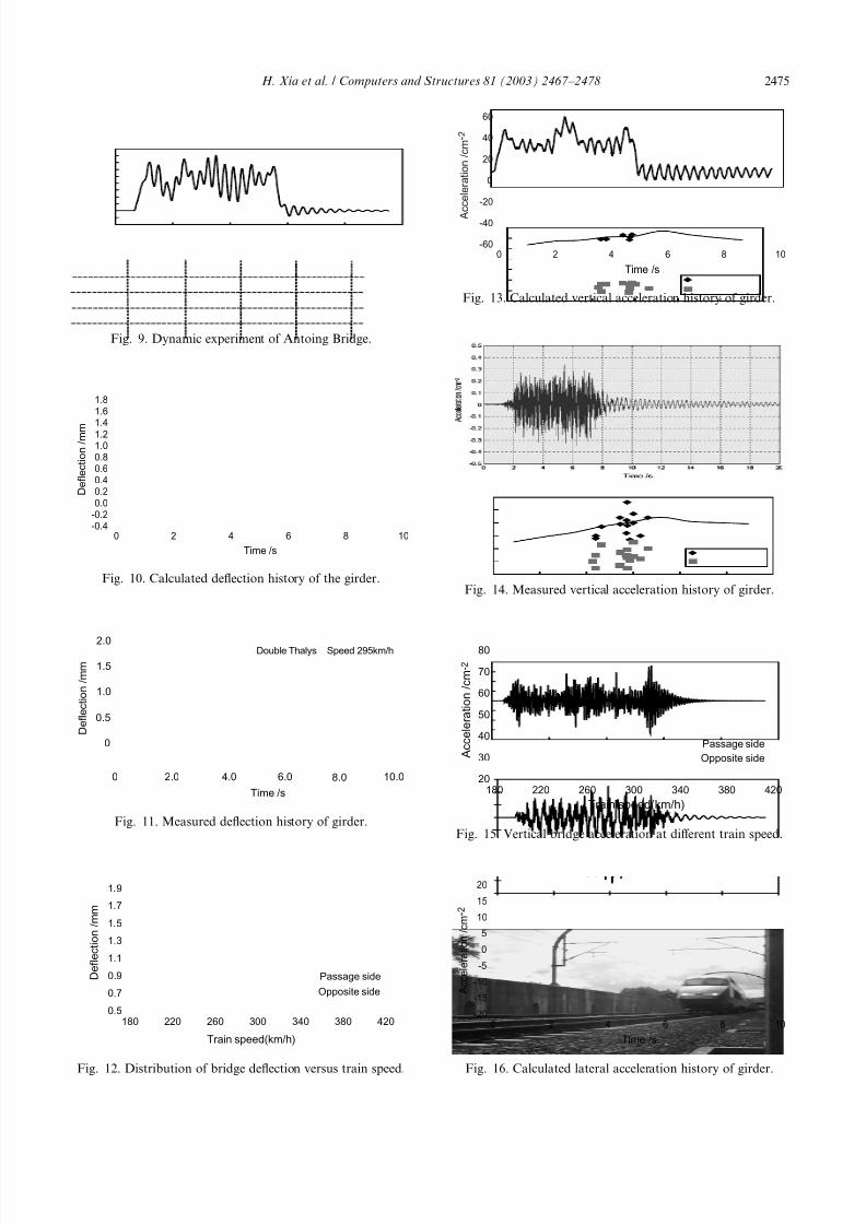
The vibration histories of calculated and measured

bridge deflections, vertical and lateral accelerations re-

spectively (Figs. 10 and 11, 13 and 14, 16 and 17) show

Fig. 4. View of the Antoing Bridge.


7/28/2019 xiahij03b


quite good similarities. It can be noticed from Figs. 12,

15 and 18 that the measured data scattered around the

corresponding calculated distribution curves versus train

speed. In other words, the calculated results are almost

at the average position of the distributed measured data

at different train speeds. The scattering of the measureddata may be owing to the randomness of the system

excitation such as the track irregularities. Generally

speaking, using the bridge-articulated-train system

model under the simplification of track model and other

assumptions, the calculated results are well in accor-

dance, both in amplitudes and in distribution tendencies,

with the in situ measured data.

(2) The cross-section deformation of the girder is

considered in the modal analysis.

According to the assumptions, the displacement, ve-

locity and acceleration of wheelsets are determined by

the following relation:Fig. 7. FE model of the U-shaped girder.

Fig. 5. Cross-section of the U-shaped girder.

Fig. 6. Prestressing tendon arrangement of the U-shaped girder.


7/28/2019 xiahij03b


Dw ¼ Db þ Di þ Dh

V w ¼ V b þ V i þ V h

Aw ¼ Ab þ Ai þ Ah

8<: ð12Þ

where the subscript w stands for wheelset, b for bridge, i

for track irregularity and h for wheelset hunting. Db, V b

and Ab are displacement, velocity and acceleration at theposition of wheelset, including three directions of lateral

movement, rolling and floating. The generalized dis-

placement Db is calculated as following:

Y b ¼ Y b0 þ R Xb0 Á h4

R X b ¼ R Xb0

Z b ¼ Z b0

8<: ð13Þ

where Y , R X and Z are the displacements in lateral, ro-

tational and vertical directions, respectively; Subscript

b0 stands for the track center on the girder deck; h4 is the

relative height difference between the deck level and the

center of the wheel axles.

In the calculation, the track irregularities are treated

as a random series with maximum amplitudes of 4.60

mm in the lateral and 5.77 mm in the vertical direction.

The wheel hunting movement has a wavelength of 32 m

and an amplitude of 3 mm.

2.4. Calculation method

The Newmark-b algorithm is used in the step-by-step

integration of the combined vehicle and bridge system.

Being unconditionally convergent, the method does not

require a special step length. The generalized displace-

ment, velocity and acceleration of the vehicle and thebridge system within a certain time step are calculated in

the program shown in Fig. 8. The convergence of the

generalized displacement of each DOF in both systems

must be ensured within the step.

3. Calculation results and their comparison to experimen-

tal data

The whole response histories of the high speed train

passing on one of the double tracks on the bridge were

simulated, by using the parameters of the real 50 m

trough PC girder and the Thalys train. The train speed

range in the calculation is 200–400 km/h and the inte-

gration time interval is 0.005 s.

The calculated and the measured modal parameters

of the girder are given in Table 1 [1].

To understand the dynamic behaviour of the bridge

under high speed trains and to verify the analytical

model, two in situ experiments on the Antoing Bridge

were carried out cooperatively by the Northern Jiaotong

University from China and the Catholic University of

Leuven, the Free University of Brussels and the Belgium

Railway Company NMBS-SNCB in Belgium. Fig. 9

shows the running high speed Thalys train on the bridgeduring the experiment.

The dynamic response histories of the bridge under

the train speed of 300 km/h and the distribution of the

maximum bridge responses versus train speed are shown

in Figs. 10–18, respectively, where the curves in solid

lines are the calculated results and the discrete symbols

are the measured data.

Within the train speed range of 200–400 km/h, the

maximum deflection of the girder is 1.79 mm, occurring

at the resonant train speed of 325 km/h, and the cor-

responding deflection-to-span ratio is 1/28,000. The

Fig. 8. Flowchart of system iteration program.

Table 1

Theoretical and experimental modal characteristics

Mode Eigenfrequency/Hz Damping ratio/% Characterization of mode

Theoretical Experimental

B1 3.19 3.19 0.63 First bending (symmetric)

T1 3.95 3.87 2.98 First torsional (symmetric)

S1 6.70 6.84 2.74 First bending of cross-section (symmetric)

B2 9.20 8.77 2.24 First anti-symmetric bending

T2 10.39 10.56 1.83 Second torsional (anti-symmetric)

S2 12.33 12.46 1.52 Second bending of cross-section (anti-symmetric)

B3 14.57 18.56 1.52 Second symmetric bending

B4 18.44 19.28 156 Second anti-symmetric bending


7/28/2019 xiahij03b


Fig. 9. Dynamic experiment of Antoing Bridge.

-0.4-0.20.00.20.40.60.81.01.21.41.61.8

0 2 4 6 8 10

Time /s

D e f l e c t i o n / m m

Fig. 10. Calculated deflection history of the girder.

Double Thalys Speed 295km/h

0 4.02.0 6.0 8.0 10.0

0

0.5

1.0

1.5

2.0


Time /s

Fig. 11. Measured deflection history of girder.

0 5

0 7

0 9

1 1

1 3

1 5

1 7

1 9

180 220 260 300 340 380 420

Passage side

Opposite side

.

.

.

.

.

.

.

.


Train speed(km/h)

Fig. 12. Distribution of bridge deflection versus train speed.

-60

-40

-20

0

20

40

60

0 2 4 6 8 10

Time /s

A

c c e l e r a t i o n / c m - 2

Fig. 13. Calculated vertical acceleration history of girder.

Fig. 14. Measured vertical acceleration history of girder.

20

30

40

50

60

70

80

180 220 260 300 340 380 420

Passage side

Opposite side

Train speed(km/h)

A c c e l e r a t i o n / c m - 2

Fig. 15. Vertical bridge acceleration at different train speed.

-20

-15

-10

-5

0

5

10

15

20

0 2 4 6 8 10

Time /s


Fig. 16. Calculated lateral acceleration history of girder.


7/28/2019 xiahij03b


maximum vertical acceleration of the girder is 0.65

m/s2.

The lateral amplitudes and the accelerations are very

small, and both of them increase with the train speed. In

the train speed range lower than 325 km/h, the maxi-

mum lateral amplitude is 0.145 mm and the maximum

lateral acceleration is 0.167 m/s2.

Figs. 19 and 20 show the vertical and lateral car-body

accelerations of the locomotives and the articulated ve-

hicle under the train speed of 300 km/h. Fig. 21 shows

the distribution of the maximum car-body accelerations

of the locomotives and the vehicles.

The lateral car-body accelerations of both locomo-tives and vehicles increase with the train speed. In the

train speed range of 200–400 km/h, the maximum lateral

car-body accelerations of the locomotives and the vehi-

cles are 1.31 and 0.77 m/s2, respectively. Both the ver-

tical car-body accelerations of the locomotives and the

vehicles are smaller than 0.65 m/s2. The maximum ver-

tical car-body accelerations of locomotives and vehicles

occur at the resonant train speed of 325 km/h.

The study on the 20 vehicles of the double Thalys

train reveals that both the lateral and the vertical car-

body accelerations of the locomotives are greater than

those of the articulated vehicles. The distributions of the

maximum car-body accelerations of the vehicles are

shown in Figs. 22 and 23, in which L denotes locomo-

tive, T transition carriage and P articulated vehicles. The

car-body accelerations of the vehicles of the 4th and the5th articulated vehicles are 80–85% in vertical and 70–

80% in lateral of those of the transition carriages. These

values are similar to those of the 200 km/h railway in

China.

The comparisons of the vibration histories of bridge

deflections, vertical and lateral accelerations respectively

between Figs. 10 and 11, 13 and 14, 16 and 17 show

quite good similarities. It can be noticed from Figs. 12,

15 and 18 that the measured data scattered around the

corresponding calculated distribution curves versus train

speed. In other words, the calculated results are almost

at the average position of the distributed measured data

-90

-60

-30

0

30

60

90

0 2 4 6 8 10

Time /s

A c

c e l e r a t i o n / c m - 2

Fig. 19. Vehicle lateral acceleration history.

-60

-40

-20

0

20

40

60

0 2 4 6 8 10

Time /s

A c c e

l e r a t i o n / c m - 2

Fig. 20. Vehicle vertical acceleration history.

Fig. 17. Measured lateral acceleration history of girder.

180 220 260 300 340 380 420

0

4

8

12

16

20

24

Train speed(km/h)

A c c e l e r a t i o n / c m -

2

Fig. 18. Lateral bridge acceleration at different train speed.

20

40

60

80

100

120

140

180 220 260 300 340 380 420

Time


Loconotive lateral

Loconotive lateral

Vehicle lateralVehicle lateral

Fig. 21. Distribution of vehicle acceleration versus train speed.


7/28/2019 xiahij03b


at different train speeds. The scattering of the measured

data may be owing to the randomness of the system

excitation such as the track irregularities. Generally

speaking, using the bridge-articulated-train system

model under the simplification of track model and other

assumptions, the calculated results are well in accor-

dance, both in amplitudes and in distribution tendencies,

with the in situ measured data.

Compared with the measured results in China, where

the trains with non-articulated vehicles are used, the

vehicle accelerations are almost the same, while the

bridges responses such as deflection–span ratios, am-

plitudes and accelerations are smaller [16].

In fact, for normal bridges of this length, it is usually

more convenient to obtain good results of bridge de-

flections by using only a load representation of the train

[1]. While for the other dynamic responses, such as the

accelerations of the bridges, the dynamic responses of

the running vehicles, the complete vehicle–bridge system

is necessary.

4. Conclusions

The following conclusions can be drawn up from this

paper:

(1) The dynamic analytical model of the bridge-articu-

lated-train system and the computer simulation

method proposed in this paper can well reflect the

main vibration characteristics of the bridge and the

articulated train vehicle.

(2) The calculated results are well in accordance, both in

response curves, in amplitudes and in distribution

tendencies, with the in situ measured data, which

verified the effectiveness of the analytical model

and the computer simulation method.

(3) The Antoing Bridge has perfect dynamic character-

istics. The ratio of deflection-to-span of the AntoingBridge is smaller than that of the similar bridges in

China. The deflections of the girder, the lateral and

vertical accelerations of the girder and the car body

are in accordance with the currently recognized

safety and comfort standards of bridges and running

train vehicles.

(4) The articulated train vehicles have a rather good

running property at high speed, which also helps

to reduce the impact on the bridge structures.

Acknowledgements

This study is sponsored by the National Natural

Science Foundation of China (grant no. 50078001) and

the Bilateral Research Project (BIL98/09) from the

Ministry of the Flemish Community of Belgium.

References

[1] De Roeck G, Maeck J, Teughels A. Train–bridge interac-

tion validation of numerical models by experiments onhigh-speed railway bridge in Antoing, TIVC’2001, Beijing.

[2] Diana G, Cheli F. Dynamic interaction of railway systems

with large bridges. Veh Syst Dynam 1989;18:71–106.

[3] Fryba L. Vibration of solids and structures under moving

loads. Groningen: Noordhoff International Publishing;

1972.

[4] Fafard M. Dynamics of bridge vehicle interaction. In: Proc

EURODYN’93. Rotterdam: Balkema; 1993. p. 951–60.

[5] Klasztorny M. Vertical vibration of a multi-span bridge

under a train moving at high speed. In: Proc EURO-

DYN’99. Rotterdam: Balkema; 1999. p. 651–6.

[6] Li SL, Wang WD. Dynamic analysis of articulated vehicles

considering car-body elasticity. J China Railway Sci 1997;

18(2):77–85.

[7] Matsuuta AA. Study of dynamic behaviors of bridge

girders for high speed railway. J JSCE 1976;256:35–47.

[8] Shen G, Lu ZG, Hu YS. Nonlinear curving simulation for

high speed articulated train. J China Railway Soc 1997;

(Suppl):9–14.

[9] Sridharan N, Mallik AK. Numerical analysis of vibration

of beams subjected to moving loads. J Sound Vib

1979;65:147–50.

[10] Wiriyachai A, Chu KH, Garg K. Bridge impact due to

wheel and track irregularities. J Engng Mech ASCE

1982;108:648–67.

[11] Xia H. Dynamic interaction of vehicles and structures.

Beijing: Science Press; 2002.

P P P P P P P P P P P P0

20

40

60

80

100

120

140Lateral acceleration of car-body /cms

-2

L L LLT T T T

Fig. 22. Maximum lateral accelerations of vehicles.

0

20

40

60Vertical acceleration of car-body /cms-2

P P P P P P P P P P P P

L L LLT T T T

Fig. 23. Maximum vertical accelerations of vehicles.


7/28/2019 xiahij03b


[12] Xia H, Xu YL, Chan THT. Dynamic interaction of long

suspension bridges with running trains. Int J Sound Vibrat

2000;237(2):263–80.

[13] Xia H, De Roeck G, Zhang HR, Zhang N. Dynamic

analysis of train–bridge system and its application in steel

girder reinforcement. J Comput Struct 2001;79:1851–60.

[14] Yang YB, Yau JD. Vehicle–bridge interaction element fordynamic analysis. J Struct Engng ASCE 1997;123(11):

1512–8.

[15] Zhai WM. Study on coupled vertical dynamics of vehicle–

track system. J China Railway Soc 1997;(8):16–21.

[16] Zhang N. Dynamic interaction analysis of vehicle–

bridge system under articulated high speed trains. Doc-

toral Thesis, Beijing, Northern Jiaotong University,

2002.

[17] European Rail Research Institute, List of ERRI publica-tions, January 2003 (available on website http://www.

eri.nl).


http://www.eri.nl/

http://www.eri.nl/

http://www.eri.nl/

http://www.eri.nl/

http://www.eri.nl/

Documents

xiahij03b