2008 4th International IEEE Conference "Intelligent Systems"

xftsp: a Tool for Time Series Prediction byMeans of Fuzzy Inference Systems

Federico Montesino, Amaury Lendasse and Angel Barriga

Abstract- A new software tool for time series prediction bymeans of fuzzy inference systems is reported. This tool, namedxftsp, implements a novel methodology for time series predictionbased on methods for automatic fuzzy systems identificationand supervised learning combined with statistical methods fornonparametric residual variance estimation. xftsp is designedas a tool integrated in the Xfuzzy development environmentfor fuzzy systems. Experiments carried out on a number oftime series benchmarks show the advantages of xftsp in termsof both accuracy and computational requirements as comparedagainst Least-Squared Support Vector Machines, an establishedtechnique in the field of time series prediction.

Index Terms- Time series prediction, Fuzzy inference, Su­pervised learning, Nonparametric regression, Residual varianceestimation, Least-squared support vector machines

I. INTRODUCTION

In the past, conventional statistical techniques such as AR,ARMA and derived models have been extensively used forforecasting. However, these techniques have limited capa­bilities for modeling time series data, and more advancednonlinear methods including neural networks, evolutionaryalgorithms and other soft computing techniques have beenoften applied with success [I].

Fuzzy logic based modeling techniques are appealingbecause of their interpretability and potential to addressa broad spectrum of problems. The application of fuzzyinference systems to time series modeling and predictiondates back to [2], in which the authors develop the wellknown learn from examples identification algorithm for fuzzyinference systems and use the Mackey-Glass time series as avalidation case. Nevertheless, despite its good performancein terms of accuracy and interpretability, fuzzy systems haveseen little application in the field of time series predictionas compared to other nonlinear modeling techniques such asneural networks and support vector machines.

Recently, a methodology framework has been proposedfor the long-term prediction of time-series by means of fuzzy

Federico Montesino Pouzols is with the Microelectronics Institute ofSeville, CSIC, Scientific Research CounciL Avda. Reina Mercedes sIn. Edif.CICA. E-41012 Seville, Spain (phone: +34-955-056-666; fax: +34-955-056­686; email: fedemp@imse.cnm.es).

Amaury Lendasse is with the Laboratory of Computer and InformationScience of the Helsinky University of Technology. P.O. Box 5400, FIN­02015 HUT, Finland (phone: +358-9-451 3267; fax: +358-9-451 3277;email: lendasse@cis.hut.fi).

Angel Barriga Barros is with the Department of Electronics and Electro­magnetism of the University of Seville, E-41012, Spain (phone: +34-955­056-666; fax: +34-955-056-686; email: barriga@us.es).

This work has been supported in part by project TEC2005-04359/MICfrom the Spanish Ministry of Education and Science as well as projectTIC2006-635 and grant IAC07-I-0205:33080 from the Andalusian regionalGovernment.

systems [3]. This paper introduces a tool that implements thecited methodology in an open and modular way. Experimen­tal results are compared against the reference implementationof a methodology commonly applied in the time seriesprediction field, least-squared support vector machines.

II. NONPARAMETRIC RESIDUAL VARIANCE

ESTIMATION: DELTA TEST

Nonparametric residual variance estimation (NRVE) is awell-known technique in statistics and machine learning,finding many applications in nonlinear modeling [4].

Delta Test (DT) is a NRVE method for estimating thelowest mean square error (MSE) that can be achieved bya model without overfitting the training set [4]. Given Nmultiple input-single output pairs, (Xi, Yi) E RM X R, thetheory behind the DT method considers that the mappingbetween Xi and Yi is given by the following expression:

Yi == !(Xi) + ri,

where ! is an unknown perfect fitting model and ri is thenoise. DT is based on hypothesis coming from the continuityof the regression function. When two inputs x and x' areclose, the continuity of the regression function implies thatoutputs ! (x) and ! (x') will be close enough. When thisimplication does not hold, it is due to the influence of thenoise.

Let us denote the first nearest neighbor of the point Xi inthe set {Xl, ... , XN} by XNN. Then the DT, ~, is defined asfollows:

1 N 2

0= 2N L IYNN(i) - Yil 'i=1

where YNN(i) is the output corresponding to XNN(i)' Fora proof of convergence, refer to [5]. DT has been shownto be a robust method for estimating the lowest possiblemean squared error (MSE) of a nonlinear model withoutoverfitting. DT is useful for evaluating nonlinear correlationsbetween random variables, namely, input and output pairs.This method will be used for a priori input selection.

III. PREDICTION METHODOLOGY

Consider a discrete time series as a vector, fj

Yl, Y2, ... ,Yt -1 , Yt, that represents an ordered set of values,where t is the number of values in the series. The problemof predicting one future value, Yt+ 1, using an autoregressivemodel (autoregressor) with no exogenous inputs can be statedas follows:

978-1-4244-1739-1/08/$25.00 © 2008 IEEE 2-2

Authorized licensed use limited to: Teknillinen Korkeakoulu. Downloaded on December 9, 2009 at 07:52 from IEEE Xplore. Restrictions apply.

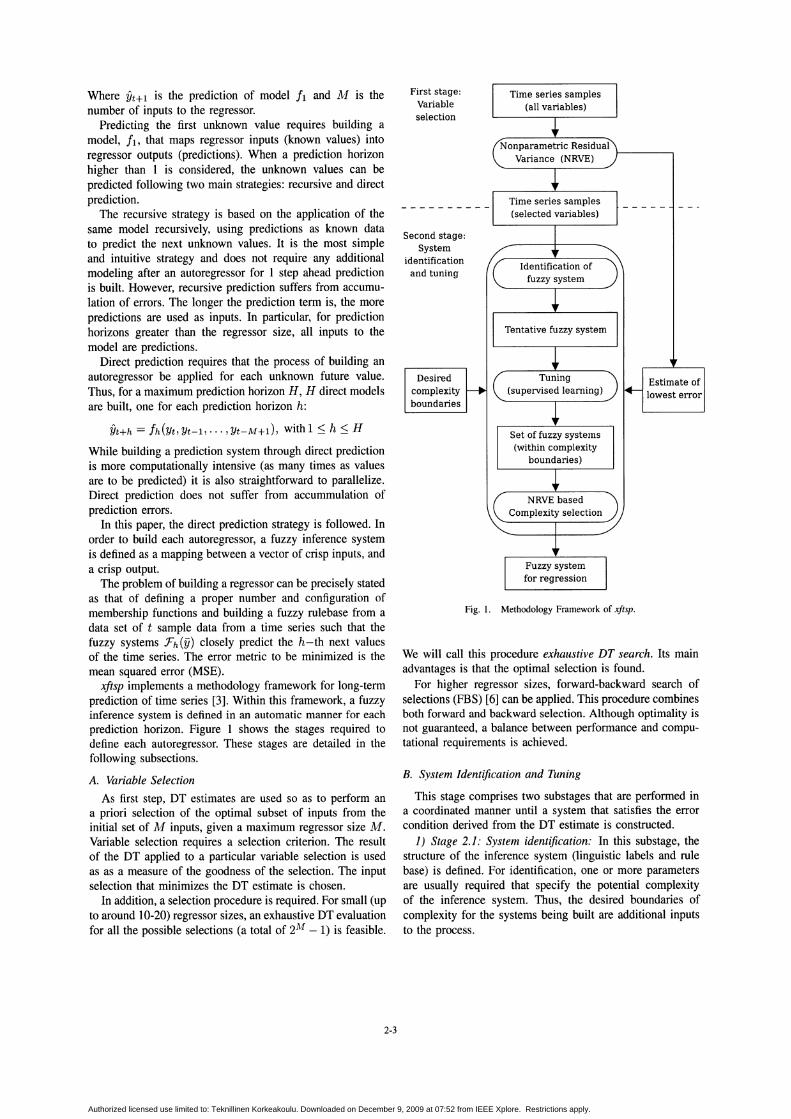
Nonparametric ResidualVariance (NRVE)

We will call this procedure exhaustive DT search. Its mainadvantages is that the optimal selection is found.

For higher regressor sizes, forward-backward search ofselections (FBS) [6] can be applied. This procedure combinesboth forward and backward selection. Although optimality isnot guaranteed, a balance between performance and compu­tational requirements is achieved.

Estimate oflowest error

Desiredcomplexityboundaries

Fig. 1. Methodology Framework of xftsp.

Set of fuzzy systelns(within complexity

boundaries)

Second stage:System

identificationand tuning

First stage:Variableselection

B. System Identification and Tuning

This stage comprises two substages that are performed ina coordinated manner until a system that satisfies the errorcondition derived from the DT estimate is constructed.

1) Stage 2.1: System identification: In this substage, thestructure of the inference system (linguistic labels and rulebase) is defined. For identification, one or more parametersare usually required that specify the potential complexityof the inference system. Thus, the desired boundaries ofcomplexity for the systems being built are additional inputsto the process.

Where Yt+l is the prediction of model il and M is thenumber of inputs to the regressor.

Predicting the first unknown value requires building amodel, ib that maps regressor inputs (known values) intoregressor outputs (predictions). When a prediction horizonhigher than 1 is considered, the unknown values can bepredicted following two main strategies: recursive and directprediction.

The recursive strategy is based on the application of thesame model recursively, using predictions as known datato predict the next unknown values. It is the most simpleand intuitive strategy and does not require any additionalmodeling after an autoregressor for 1 step ahead predictionis built. However, recursive prediction suffers from accumu­lation of errors. The longer the prediction term is, the morepredictions are used as inputs. In particular, for predictionhorizons greater than the regressor size, all inputs to themodel are predictions.

Direct prediction requires that the process of building anautoregressor be applied for each unknown future value.Thus, for a maximum prediction horizon H, H direct modelsare built, one for each prediction horizon h:

Yt+h == ih(Yt, Yt-l, ... ,Yt-M+l), with 1 ::; h ::; H

While building a prediction system through direct predictionis more computationally intensive (as many times as valuesare to be predicted) it is also straightforward to parallelize.Direct prediction does not suffer from accummulation ofprediction errors.

In this paper, the direct prediction strategy is followed. Inorder to build each autoregressor, a fuzzy inference systemis defined as a mapping between a vector of crisp inputs, anda crisp output.

The problem of building a regressor can be precisely statedas that of defining a proper number and configuration ofmembership functions and building a fuzzy rulebase from adata set of t sample data from a time series such that thefuzzy systems fh (y) closely predict the h-th next valuesof the time series. The error metric to be minimized is themean squared error (MSE).

xftsp implements a methodology framework for long-termprediction of time series [3]. Within this framework, a fuzzyinference system is defined in an automatic manner for eachprediction horizon. Figure 1 shows the stages required todefine each autoregressor. These stages are detailed in thefollowing subsections.

A. Variable Selection

As first step, DT estimates are used so as to perform ana priori selection of the optimal subset of inputs from theinitial set of M inputs, given a maximum regressor size M.Variable selection requires a selection criterion. The resultof the DT applied to a particular variable selection is usedas as a measure of the goodness of the selection. The inputselection that minimizes the DT estimate is chosen.

In addition, a selection procedure is required. For small (upto around 10-20) regressor sizes, an exhaustive DT evaluationfor all the possible selections (a total of 2!v[ - 1) is feasible.

2-3

Authorized licensed use limited to: Teknillinen Korkeakoulu. Downloaded on December 9, 2009 at 07:52 from IEEE Xplore. Restrictions apply.

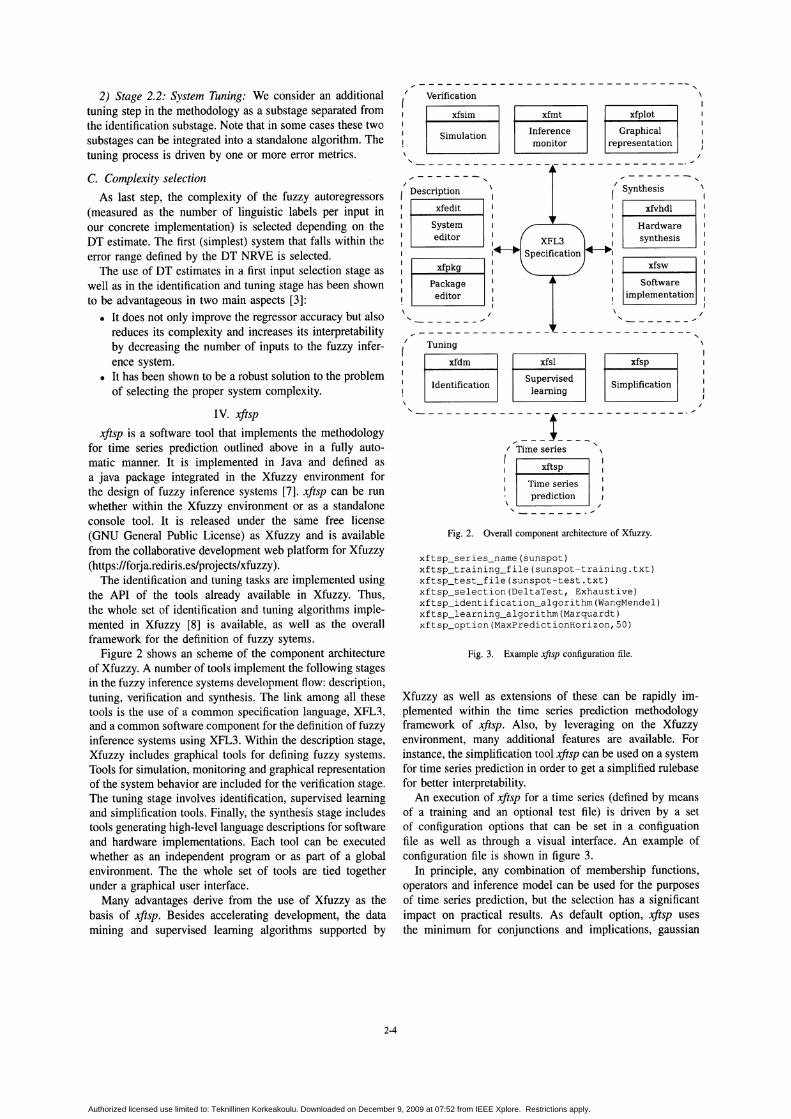
Fig. 2. Overall component architecture of Xfuzzy.

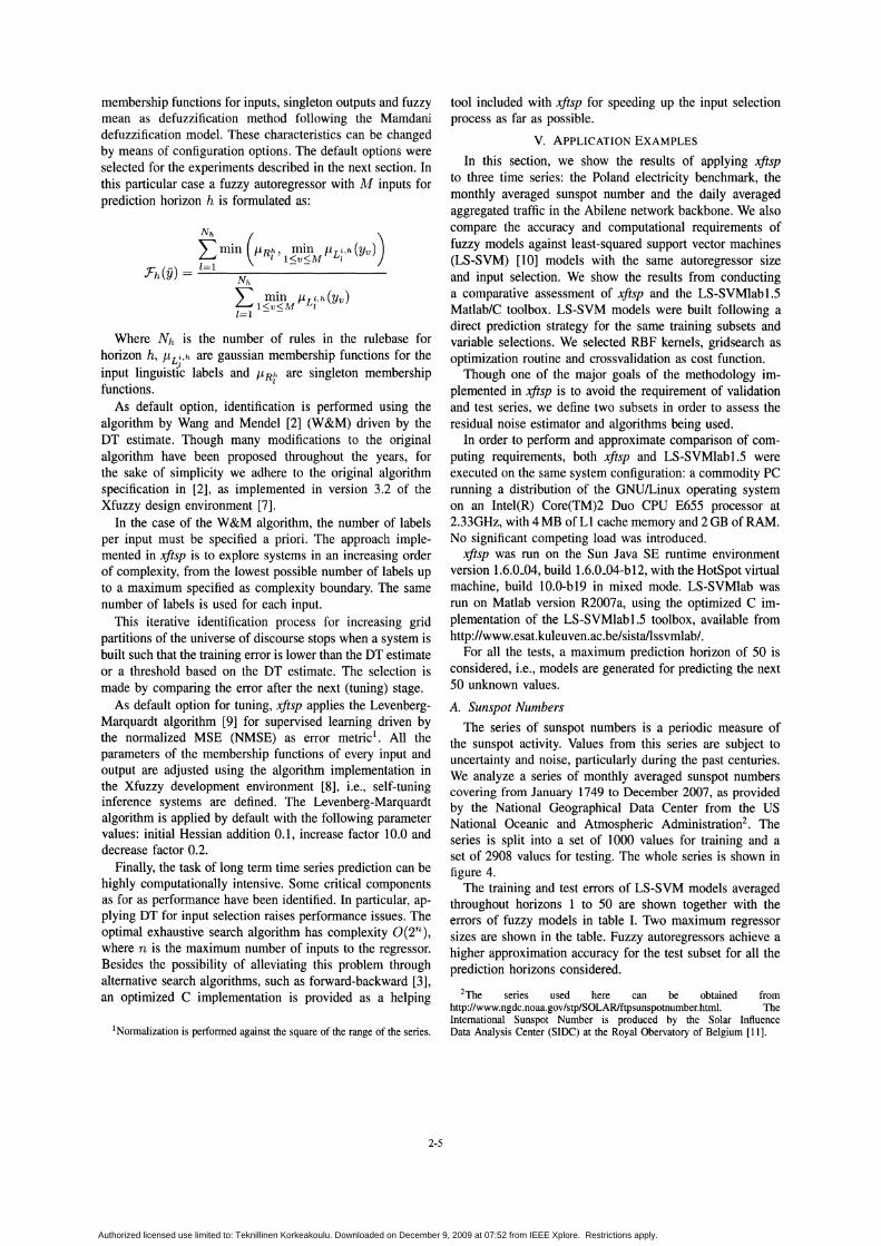
Fig. 3. Example xjisp configuration file.

,,-------------------------------,

xfsp

xfplot

Simplification

Graphicalrepresentation

xfmt

xfsl

Inferencemonitor

Time seriesprediction

Supervisedlearning

xfsim

xfdm

Simulation

Identification

Verification

Tuning

\

III

II,

I

, - - - - - - - - - - - - - - - - - - - - - - - - - - - - - _. "------- , ,,-------,

I \ ( SynthesisDescription

xfedit xfvhdl

System Hardwareeditor synthesis

xfpkg xfsw

Package Softwareeditor implementation, ,

, I , I-------""" -------*"'"

\

II

III,\. --------------1--------------- ~ I

I ;"Tim~ ;eri;s- - - '\

f Ixftsp I

II,

I,------_."

~-------------------------------,

xftsp_series_name(sunspot)xftsp_training_file(sunspot-training.txt)xftsp_test_file(sunspot-test.txt)xftsp_selection(DeltaTest, Exhaustive)xftsp_identification_algorithm(WangMendel)xftsp_learning_algorithm(Marquardt)xftsp_option(MaxPredictionHorizon,50)

Xfuzzy as well as extensions of these can be rapidly im­plemented within the time series prediction methodologyframework of xftsp. Also, by leveraging on the Xfuzzyenvironment, many additional features are available. Forinstance, the simplification tool xftsp can be used on a systemfor time series prediction in order to get a simplified rulebasefor better interpretability.

An execution of xftsp for a time series (defined by meansof a training and an optional test file) is driven by a setof configuration options that can be set in a configuationfile as well as through a visual interface. An example ofconfiguration file is shown in figure 3.

In principle, any combination of membership functions,operators and inference model can be used for the purposesof time series prediction, but the selection has a significantimpact on practical results. As default option, xftsp usesthe minimum for conjunctions and implications, gaussian

2) Stage 2.2: System Tuning: We consider an additionaltuning step in the methodology as a substage separated fromthe identification substage. Note that in some cases these twosubstages can be integrated into a standalone algorithm. Thetuning process is driven by one or more error metrics.

C. Complexity selection

As last step, the complexity of the fuzzy autoregressors(measured as the number of linguistic labels per input inour concrete implementation) is selected depending on theDT estimate. The first (simplest) system that falls within theerror range defined by the DT NRVE is selected.

The use of DT estimates in a first input selection stage aswell as in the identification and tuning stage has been shownto be advantageous in two main aspects [3]:

• It does not only improve the regressor accuracy but alsoreduces its complexity and increases its interpretabilityby decreasing the number of inputs to the fuzzy infer­ence system.

• It has been shown to be a robust solution to the problemof selecting the proper system complexity.

IV. xftsp

xftsp is a software tool that implements the methodologyfor time series prediction outlined above in a fully auto­matic manner. It is implemented in Java and defined asa java package integrated in the Xfuzzy environment forthe design of fuzzy inference systems [7]. xftsp can be runwhether within the Xfuzzy environment or as a standaloneconsole tool. It is released under the same free license(GNU General Public License) as Xfuzzy and is availablefrom the collaborative development web platform for Xfuzzy(https://forja.rediris.es/projects/xfuzzy).

The identification and tuning tasks are implemented usingthe API of the tools already available in Xfuzzy. Thus,the whole set of identification and tuning algorithms imple­mented in Xfuzzy [8] is available, as well as the overallframework for the definition of fuzzy sytems.

Figure 2 shows an scheme of the component architectureof Xfuzzy. A number of tools implement the following stagesin the fuzzy inference systems development flow: description,tuning, verification and synthesis. The link among all thesetools is the use of a common specification language, XFL3,and a common software component for the definition of fuzzyinference systems using XFL3. Within the description stage,Xfuzzy includes graphical tools for defining fuzzy systems.Tools for simulation, monitoring and graphical representationof the system behavior are included for the verification stage.The tuning stage involves identification, supervised learningand simplification tools. Finally, the synthesis stage includestools generating high-level language descriptions for softwareand hardware implementations. Each tool can be executedwhether as an independent program or as part of a globalenvironment. The the whole set of tools are tied togetherunder a graphical user interface.

Many advantages derive from the use of Xfuzzy as thebasis of xftsp. Besides accelerating development, the datamining and supervised learning algorithms supported by

2-4

Authorized licensed use limited to: Teknillinen Korkeakoulu. Downloaded on December 9, 2009 at 07:52 from IEEE Xplore. Restrictions apply.

membership functions for inputs, singleton outputs and fuzzymean as defuzzification method following the Mamdanidefuzzification model. These characteristics can be changedby means of configuration options. The default options wereselected for the experiments described in the next section. Inthis particular case a fuzzy autoregressor with M inputs forprediction horizon h is formulated as:

Where Nh is the number of rules in the rulebase forhorizon h, J-LLi,h are gaussian membership functions for theinput linguisti~ labels and J-LRh are singleton membership

lfunctions.

As default option, identification is performed using thealgorithm by Wang and Mendel [2] (W&M) driven by theDT estimate. Though many modifications to the originalalgorithm have been proposed throughout the years, forthe sake of simplicity we adhere to the original algorithmspecification in [2], as implemented in version 3.2 of theXfuzzy design environment [7].

In the case of the W&M algorithm, the number of labelsper input must be specified a priori. The approach imple­mented in xftsp is to explore systems in an increasing orderof complexity, from the lowest possible number of labels upto a maximum specified as complexity boundary. The samenumber of labels is used for each input.

This iterative identification process for increasing gridpartitions of the universe of discourse stops when a system isbuilt such that the training error is lower than the DT estimateor a threshold based on the DT estimate. The selection ismade by comparing the error after the next (tuning) stage.

As default option for tuning, xftsp applies the Levenberg­Marquardt algorithm [9] for supervised learning driven bythe normalized MSE (NMSE) as error metric I. All theparameters of the membership functions of every input andoutput are adjusted using the algorithm implementation inthe Xfuzzy development environment [8], i.e., self-tuninginference systems are defined. The Levenberg-Marquardtalgorithm is applied by default with the following parametervalues: initial Hessian addition 0.1, increase factor 10.0 anddecrease factor 0.2.

Finally, the task of long term time series prediction can behighly computationally intensive. Some critical componentsas for as performance have been identified. In particular, ap­plying DT for input selection raises performance issues. Theoptimal exhaustive search algorithm has complexity 0 (2n ),

where n is the maximum number of inputs to the regressor.Besides the possibility of alleviating this problem throughalternative search algorithms, such as forward-backward [3],an optimized C implementation is provided as a helping

1Normalization is performed against the square of the range of the series.

2-5

tool included with xftsp for speeding up the input selectionprocess as far as possible.

Y. ApPLICATION EXAMPLES

In this section, we show the results of applying xftspto three time series: the Poland electricity benchmark, themonthly averaged sunspot number and the daily averagedaggregated traffic in the Abilene network backbone. We alsocompare the accuracy and computational requirements offuzzy models against least-squared support vector machines(LS-SYM) [10] models with the same autoregressor sizeand input selection. We show the results from conductinga comparative assessment of xftsp and the LS-SYMlab1.5Matlab/C toolbox. LS-SVM models were built following adirect prediction strategy for the same training subsets andvariable selections. We selected RBF kernels, gridsearch asoptimization routine and crossvalidation as cost function.

Though one of the major goals of the methodology im­plemented in xftsp is to avoid the requirement of validationand test series, we define two subsets in order to assess theresidual noise estimator and algorithms being used.

In order to perform and approximate comparison of com­puting requirements, both xftsp and LS-SYMlab1.5 wereexecuted on the same system configuration: a commodity PCrunning a distribution of the GNUILinux operating systemon an Intel(R) Core(TM)2 Duo CPU E655 processor at2.33GHz, with 4 MB of Ll cache memory and 2 GB of RAM.No significant competing load was introduced.

xftsp was run on the Sun Java SE runtime environmentversion 1.6.0_04, build 1.6.0_04-b12, with the HotSpot virtualmachine, build 10.0-b19 in mixed mode. LS-SYMlab wasrun on Matlab version R2007a, using the optimized C im­plementation of the LS-SYMlab1.5 toolbox, available fromhttp://www.esat.kuleuven.ac.be/sista/lssvmlab/.

For all the tests, a maximum prediction horizon of 50 isconsidered, Le., models are generated for predicting the next50 unknown values.

A. Sunspot Numbers

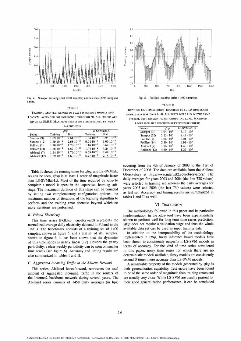
The series of sunspot· numbers is a periodic measure ofthe sunspot activity. Values from this series are subject touncertainty and noise, particularly during the past centuries.We analyze a series of monthly averaged sunspot numberscovering from January 1749 to December 2007, as providedby the National Geographical Data Center from the USNational Oceanic and Atmospheric Administration2 . Theseries is split into a set of 1000 values for training and aset of 2908 values for testing. The whole series is shown infigure 4.

The training and test errors of LS-SYM models averagedthroughout horizons 1 to 50 are shown together with theerrors of fuzzy models in table I. Two maximum regressorsizes are shown in the table. Fuzzy autoregressors achieve ahigher approximation accuracy for the test subset for all theprediction horizons considered.

2The series used here can be obtained fromhttp://www.ngdc.noaa.gov/stp/SOLARlftpsunspotnumber.html. TheInternational Sunspot Number is produced by the Solar InfluenceData Analysis Center (SIDC) at the Royal Obervatory of Belgium [11].

Authorized licensed use limited to: Teknillinen Korkeakoulu. Downloaded on December 9, 2009 at 07:52 from IEEE Xplore. Restrictions apply.

~ ~

1 It

~~ ;, II , ~ iI

I 1 I :_ aW~.,- ,14001000 1200800

Days

600400200

0.7

1.3 ~.~~~ .. ~ .. ~~,~~~ .. ~ ~~~~~~~~ ~ ....:.;~~~~~~ ~~~~~~~~~~,~~~~.~~ .. ~~~~~~~~.~,~'lIlt_~~.~ .. ~~:~.~ ... ~.~~.~~.~~.~~. .~ .. ~. ~~~.,

"'0

~ 1.1

~~'0'.9~ 0.9

0.8

1.4 r-----,----r---.------,----r---r------,

3000250020001500

Months

1000500o

o

300

250

~200

"8::lc

150(5~C::l

CI)

100

50

Fig. 4. Sunspot: training (first 1000 samples) and test (last 2098 samples)series.

Fig. 5. PolElec: training series (1400 samples).

TABLE I

TRAINING AND TEST ERRORS OF FUZZY INFERENCE MODELS AND

LS-SVM, AVERAGED FOR HORIZONS 1 THROUGH 50. ALL ERRORS ARE

GIVEN AS NMSE. MAXIMUM REGRESSOR SIZE SPECIFIED BETWEEN

PARENTHESIS.

xjtspTest

LS-SVMlab1.5

TABLE II

RUNNING TIME (IN SECONDS) REQUIRED TO BUILD TIME SERIES

MODELS FOR HORIZONS 1-50. ALL TESTS WERE RUN ON THE SAME

SYSTEM, WITH NO SIGNIFICANT COMPETING LOAD. MAXIMUM

REGRESSOR SIZE SPECIFIED BETWEEN PARENTHESIS.

3.10.105

2.42 .105

3.04.105

9.91 . 105

1.40 .105

1.27 . 105

LS-SVMlab1.5xjtsp1.04 . 104

1.22 .104

1.05 . 104

2.30.104

1.75.103

4.69.103

Sunspot (9)Sunspot (12)Po1E1ec (7)PolElec (14)Abilenel (7)Abilenel (12)

Series

Test3.28.10- 2

3.02.10- 2

3.57.10- 2

3.24.10-2

2.47.10- 2

2.15.10- 2

Training1.34.10-2

9.64.10-3

1.16.10-2

1.04.10-2

8.58.10-3

6.77.10- 3

2.64,10- 2

2.63.10- 2

1.78.10- 2

1.82.10-2

1.73.10-2

1.50.10-2

Training1.69.10-2

1.59.10-2

1.70.10-2

1.58.10-2

1.44.10-2

1.22.10-2

SeriesSunspot (9)Sunspot (12)PolElec (7)PolElec (14)Abilenel (7)Abilenel (12)

Table II shows the running times for xftsp and LS-SYMlab.As can be seen, xftsp is at least 1 order of magnitude fasterthan LS-SYMlab1.5. Most of the time required by xftsp tocomplete a model is spent in the supervised learning sub­stage. The maximum duration of this stage can be boundedby setting two complementary configuration options: themaximum number of iterations of the learning algorithm toperform and the training error decrease beyond which nomore iterations are performed.

B. Poland Electricity

This time series (PolElec henceforward) represents thenormalized average daily electricity demand in Poland in the1990's. The benchmark consists of a training set of 1400samples, shown in figure 5, and a test set of 201 samples,shown in figure 6. It has been shown that the dynamicsof this time series is nearly linear [12]. Besides the yearlyperiodicity, a clear weekly periodicity can be seen on smallertime scales (see figure 6). Accuracy and timing results arealso summarized in tables I and II.

C. Aggregated Inconling Traffic in the Abilene Network

This series, AbileneI henceforward, represents the totalamount of aggregated incoming traffic in the routers ofthe Intemet2 backbone network during several years. TheAbileneI series consists of 1458 daily averages (in bps)

covering from the 4th of January of 2003 to the 31 st ofDecember of 2006. The data are available from the AbileneObservatory at http://www.internet2.edu/observatory/. Thedaily averages for years 2003 and 2004 (the first 728 values)were selected as training set, whereas the daily averages foryears 2005 and 2006 (the last 730 values) were selectedas test set. Accuracy and timing results are summarized intables I and II as well.

VI. DISCUSSION

The methodology followed in this paper and its particularimplementation in the xftsp tool have been experimentallyshown to perform well for long-term time series prediction.xftsp does not require a validation stage and thus the wholeavailable data set can be used as input training data.

In addition to the interpretability of the methodologyimplemented in xftsp, fuzzy inference based models havebeen shown to consistently outperform LS-SYM models interms of accuracy. For the kind of time series consideredin this paper, noisy time series for which there are nodeterministic models available, fuzzy models are consistentlyaround 3 times more accurate than LS-SYM models.

A remarkable property of the models generated by xftsp istheir generalization capability. Test errors have been foundto be of the same order of magnitude than training errors andare usually very close. While LS-SYM are usually praised fortheir good generalization performance, it can be concluded

2-6

Authorized licensed use limited to: Teknillinen Korkeakoulu. Downloaded on December 9, 2009 at 07:52 from IEEE Xplore. Restrictions apply.

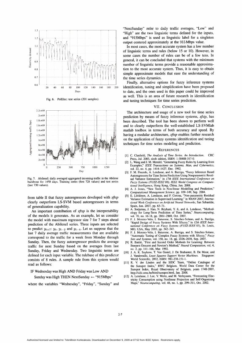
Fig. 6. PolElec: test series (201 samples).

20 40 60 80 100 120 140 160 180 200

Days

[1] C. Chatfield. The Analysis of Time Series. An Introduction. CRCPress, Jul. 2003, sixth edition, ISBN: 1-58488-317-0.

[2] L. Wang and J. M. Mendel, "Generating Fuzzy Rules by Learning fromExamples," IEEE Transactions on Systems, Man, and Cybernetics,vol. 22, no. 4, pp. 1414-1427, Dec. 1992.

[3] F. M. Pouzols, A. Lendasse, and A. Barriga, "Fuzzy Inference BasedAutoregressors for Time Series Prediction Using Nonparametric Resid­ual Variance Estimation," in 17th IEEE International Conference onFuzzy Systems (FUZZ-IEEE'08), IEEE World Congress on Computa­tional Intelligence, Hong Kong, China, Jun. 2008.

[4] A. J. Jones, "New Tools in Non-linear Modelling and Prediction,"Computational Management Science, pp. 109-149, Sep. 2004.

[5] E. LiitHiinen, A. Lendasse, and F. Corona, "Non-parametric ResidualVariance Estimation in Supervised Learning," in WANN 2007, Interna­tional Work-Conference on Artificial Neural Networks, San Sebastian,Spain, Jun. 2007, pp. 63-71.

[6] A. Sorjamaa, J. Hao, N. Reyhani, Y. Ji, and A. Lendasse, "Method­ology for Long-Term Prediction of Time Series," Neurocomputing,vol. 70, no. 16-18, pp. 2861-2869, Oct. 2007.

[7] F. J. Moreno-Ve10, I. Baturone, S. Sanchez-Solano, and A. Barriga,"Rapid Design of Fuzzy Systems With Xfuzzy," in 12th IEEE Inter­national Conference on Fuzzy Systems (FUZZ-IEEE'03), St. Louis,MO, USA, May 2003, pp. 342-347.

[8] F. 1. Moreno-Velo, I. Baturone, A. Barriga, and S. Sanchez-Solano,"Automatic Tuning of Complex Fuzzy Systems with Xfuzzy," FuzzySets and Systems, vol. 158, no. 18, pp. 2026-2038, Sep. 2007.

[9] R. Battiti, "First and Second Order Methods for Learning: BetweenSteepest Descent and Newton's Method," Neural Computation, vol. 4,no. 2, pp. 141-166, Mar. 1992.

[10] J. A. K. Suykens, T. Van Gestel, J. De Brabanter, B. De Moor, andJ. Vandewalle, Least Squares Support Vector Machines. Singapore:World Scientific, 2002, ISBN: 981-238-151-1.

[11] R. V. der Linden and the SIDC Team, "Online Catalogue ofthe Sunspot Index," RWC Belgium, World Data Center for theSunspot Index, Royal Observatory of Belgium, years 1748-2007,http://sidc.oma.be/html/sunspot.html, Jan. 2008.

[12] A. Lendasse, J. Lee, V. Wertz, and M. Verleyssen, "Forecasting Elec­tricity Consumption using Nonlinear Projection and Self-OrganizingMaps," Neurocomputing, vol. 48, no. 1, pp. 299-311, Oct. 2002.

"NextSunday" refer to daily traffic averages, "Low" and"High" are the two linguistic terms defined for the inputs,and "915Mbps" is used as linguistic label for a singletonoutput centered approximately at the 915 Mbps value.

In most cases, the most accurate system has a low numberof linguistic terms and rules (below 15 or 10). However, insome cases the number of rules can be of a few tens. Ingeneral, it can be concluded that systems with the minimumnumber of linguistic terms provide a reasonable approxima­tion to the most accurate system. Thus, it is easy to obtainsimple approximate models that ease the understanding ofthe time series dynamics.

Finally, alternative options for fuzzy inference systemsidentification, tuning and simplification have been proposedto date, and the ones used in this paper could be improvedas well. This is an area of future research in identificationand tuning techniques for time series prediction.

VII. CONCLUSION

The architecture and usage of a new tool for time seriesprediction by means of fuzzy inference systems, xfstp, hasbeen described. The tool has been shown to perform welland to clearly outperform the well-established LS-SVMlabmatlab toolbox in terms of both accuracy and speed. Byhaving a modular architecture, xftsp enables further researchon the application of fuzzy systems identification and tuningtechniques for time series modeling and prediction.

REFERENCES

12501000750

Day

500250OL.----~--~--~--'-----'------'

o

~IiM 1~r. I, ~ 1\tt n

\f\

j ... :.A

it ~N~\ 1 111 ~ nfl Mnftnlin f

U~ 1 ~ It1~

8e+08 1- ··'·+·1· .. " .1' .., .

6e+08 ~·:~·········'JIlIIlI'l:·····o

4e+08 •....:i!l:.J;:. ··IIlDlfll'Hf'lHIl

2e+08

IF Wednesday was High AND Friday was Low AND

Sunday was High THEN NextSunday ~ "915Mbps"

where the variables "Wednesday", "Friday", "Sunday" and

2.2e+09 .-------.-------.-------.------_.------_r------,

2e+09 ~................ ., : ····i····· ····ij······ ; -I

1.8e+09 1- +.... . c.... .. ;.... . : 1 ;.. ''' ~

1.6e+09

1.4e+09 ~ ··;······· .. ··········· ..·.·······Hf,·············..·,J·· : ··············1 H

1.2e+09 ~ , ....................., ····11++,···+············1+ t·······; -I.l-I

le+09 1-....... .,....... . ;·········lIb+~+··:·I+·._···:JI······· ·tl'lW·;·····

0.7

0.8

0.6

1.1

1.2

1.3

Fig. 7. AbileneI: daily averaged aggregated incoming traffic in the Abilenebackbone for 1458 days. Training series (first 728 values) and test series(last 730 values).

from table II that fuzzy autoregressors developed with xftspclearly outperform LS-SVM based autoregressors in termsof generalization capability.

An important contribution of xftsp is the interpretabilityof the models it generates. As an example, let us considerthe model with maximum regressor size 7 for 7 steps aheadprediction of the AbileneI series. Three inputs are selectedto predict Yt+7: Yt, Yt-2 and Yt-4. Let us suppose that thelast 7 daily average traffic measurements that are availablecorrespond to the traffic for a week from Monday throughSunday. Then, the fuzzy autoregressor predicts the averagetraffic for next Sunday based on the averages from lastSunday, Friday and Wednesday. Two linguistic terms aredefined for each input variable. The rulebase of this predictorconsists of 8 rules. A sample rule from this system wouldread as follows:

2-7

Authorized licensed use limited to: Teknillinen Korkeakoulu. Downloaded on December 9, 2009 at 07:52 from IEEE Xplore. Restrictions apply.