XFEM-SIMULATION OF HYDRAULIC FRACTURING IN 3D WITH

11th World Congress on Computational Mechanics (WCCM XI)5th European Conference on Computational Mechanics (ECCM V)

6th European Conference on Computational Fluid Dynamics (ECFD VI)E. Onate, J. Oliver and A. Huerta (Eds)

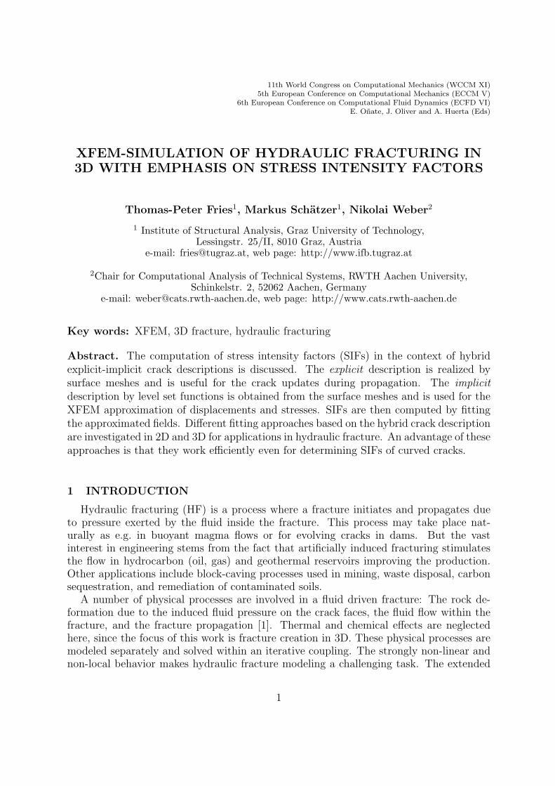
XFEM-SIMULATION OF HYDRAULIC FRACTURING IN3D WITH EMPHASIS ON STRESS INTENSITY FACTORS

Thomas-Peter Fries1, Markus Schatzer1, Nikolai Weber2

1 Institute of Structural Analysis, Graz University of Technology,Lessingstr. 25/II, 8010 Graz, Austria

e-mail: [email protected], web page: http://www.ifb.tugraz.at

2Chair for Computational Analysis of Technical Systems, RWTH Aachen University,Schinkelstr. 2, 52062 Aachen, Germany

e-mail: [email protected], web page: http://www.cats.rwth-aachen.de

Key words: XFEM, 3D fracture, hydraulic fracturing

Abstract. The computation of stress intensity factors (SIFs) in the context of hybridexplicit-implicit crack descriptions is discussed. The explicit description is realized bysurface meshes and is useful for the crack updates during propagation. The implicit

description by level set functions is obtained from the surface meshes and is used for theXFEM approximation of displacements and stresses. SIFs are then computed by fittingthe approximated fields. Different fitting approaches based on the hybrid crack descriptionare investigated in 2D and 3D for applications in hydraulic fracture. An advantage of theseapproaches is that they work efficiently even for determining SIFs of curved cracks.

1 INTRODUCTION

Hydraulic fracturing (HF) is a process where a fracture initiates and propagates dueto pressure exerted by the fluid inside the fracture. This process may take place nat-urally as e.g. in buoyant magma flows or for evolving cracks in dams. But the vastinterest in engineering stems from the fact that artificially induced fracturing stimulatesthe flow in hydrocarbon (oil, gas) and geothermal reservoirs improving the production.Other applications include block-caving processes used in mining, waste disposal, carbonsequestration, and remediation of contaminated soils.

A number of physical processes are involved in a fluid driven fracture: The rock de-formation due to the induced fluid pressure on the crack faces, the fluid flow within thefracture, and the fracture propagation [1]. Thermal and chemical effects are neglectedhere, since the focus of this work is fracture creation in 3D. These physical processes aremodeled separately and solved within an iterative coupling. The strongly non-linear andnon-local behavior makes hydraulic fracture modeling a challenging task. The extended

1

T.P. Fries, M. Schatzer, N. Weber

finite element method (XFEM) is used to deal with discontinuities and singularities whichare present in this problem due to the existence of a (fluid-filled) crack. In XFEM, addi-tional problem-specific functions (enrichments) are added to the approximation space toaccount for non-smooth solutions [3, 10, 8]. Furthermore, a hybrid explicit-implicit crackdescription is chosen which is beneficial in simulating hydraulic fracture propagation. Animplicit description by means of level-sets is employed to determine the rock deforma-tion. In contrast, a triangular surface mesh is used to describe the crack explicitly andto perform the crack update upon propagation. Another advantage of the explicit crackdescription in hydraulic fracture problems is that the fluid flow model is solved on thesurface mesh which can be a potentially curved manifold within the three dimensionaldomain [7].

In this work, a particular focus is on the efficient and reliable extraction of stress in-tensity factors (SIFs). They define the stress and displacement fields in the neighborhoodof a crack tip and are used as crack propagation criteria. There is a large number of liter-ature on different approaches. We mention energy based methods such as those based onthe J- or interaction integral, see e.g. [14, 13, 11]. Another class of methods studies thedisplacement or stress fields at the crack tip, among them the displacement extrapolationor fitting approaches, see e.g. [6, 9].

The paper is organized as follows: In Section 2, the governing equations for a hydraulicfracture problem in its basic form are presented. Models are discussed for the solid defor-mation, fluid flow, and fracture propagation. In Section 3, the XFEM formulation withan explicit-implicit crack description is described. Different approaches for the reliableevaluation of stress intensity factors are discussed in Section 4. Numerical results arepresented in Section 5.

2 GOVERNING EQUATIONS

The equations governing hydraulic fracture must account for the three main physicalphenomena of fluid flow, solid deformation, and fracture propagation. A strongly coupledpartitioned approach is used for the solution of the coupled problem.

2.1 Rock deformation

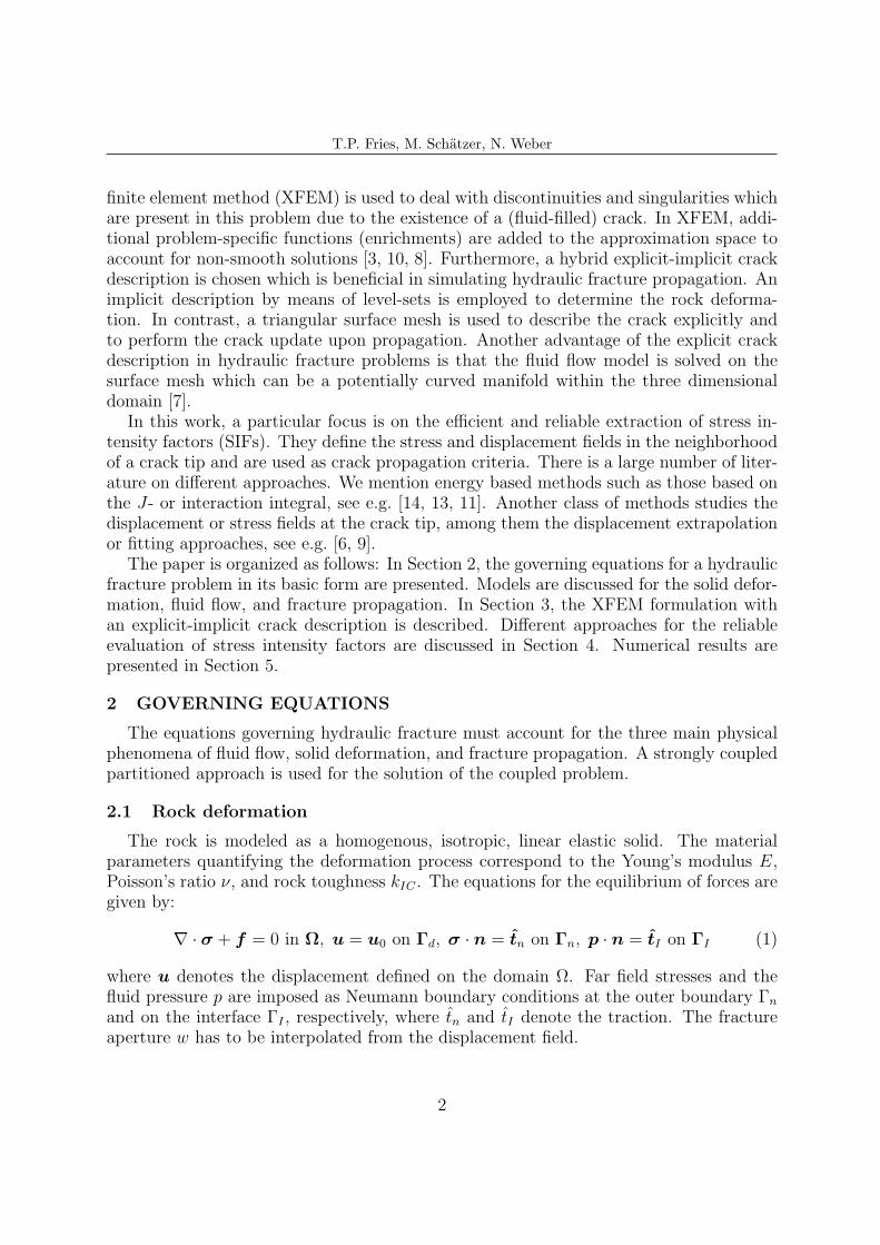
The rock is modeled as a homogenous, isotropic, linear elastic solid. The materialparameters quantifying the deformation process correspond to the Young’s modulus E,Poisson’s ratio ν, and rock toughness kIC . The equations for the equilibrium of forces aregiven by:

∇ · σ + f = 0 in Ω, u = u0 on Γd, σ · n = tn on Γn, p · n = tI on ΓI (1)

where u denotes the displacement defined on the domain Ω. Far field stresses and thefluid pressure p are imposed as Neumann boundary conditions at the outer boundary Γn

and on the interface ΓI , respectively, where tn and tI denote the traction. The fractureaperture w has to be interpolated from the displacement field.

2


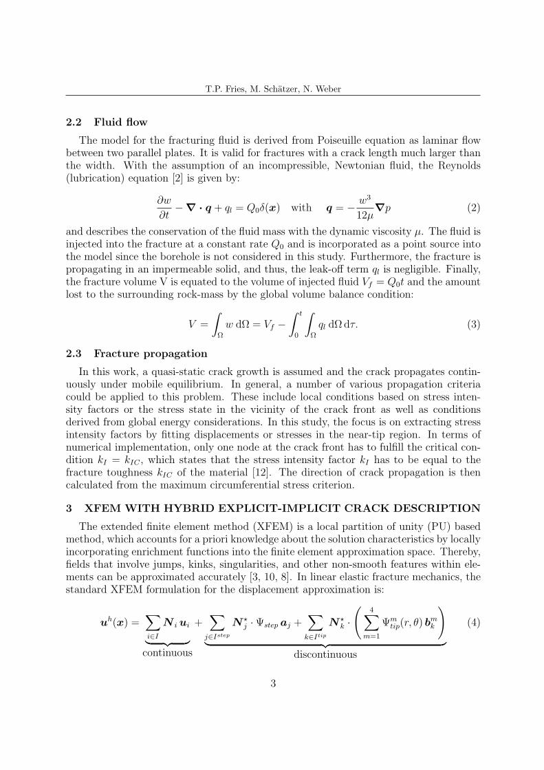
2.2 Fluid flow

The model for the fracturing fluid is derived from Poiseuille equation as laminar flowbetween two parallel plates. It is valid for fractures with a crack length much larger thanthe width. With the assumption of an incompressible, Newtonian fluid, the Reynolds(lubrication) equation [2] is given by:

∂w

∂t−∇ · q + ql = Q0δ(x) with q = −

w3

12µ∇p (2)

and describes the conservation of the fluid mass with the dynamic viscosity µ. The fluid isinjected into the fracture at a constant rate Q0 and is incorporated as a point source intothe model since the borehole is not considered in this study. Furthermore, the fracture ispropagating in an impermeable solid, and thus, the leak-off term ql is negligible. Finally,the fracture volume V is equated to the volume of injected fluid Vf = Q0t and the amountlost to the surrounding rock-mass by the global volume balance condition:

V =

∫

Ω

w dΩ = Vf −

∫ t

0

∫

Ω

ql dΩdτ. (3)

2.3 Fracture propagation

In this work, a quasi-static crack growth is assumed and the crack propagates contin-uously under mobile equilibrium. In general, a number of various propagation criteriacould be applied to this problem. These include local conditions based on stress inten-sity factors or the stress state in the vicinity of the crack front as well as conditionsderived from global energy considerations. In this study, the focus is on extracting stressintensity factors by fitting displacements or stresses in the near-tip region. In terms ofnumerical implementation, only one node at the crack front has to fulfill the critical con-dition kI = kIC , which states that the stress intensity factor kI has to be equal to thefracture toughness kIC of the material [12]. The direction of crack propagation is thencalculated from the maximum circumferential stress criterion.

3 XFEM WITH HYBRID EXPLICIT-IMPLICIT CRACK DESCRIPTION

The extended finite element method (XFEM) is a local partition of unity (PU) basedmethod, which accounts for a priori knowledge about the solution characteristics by locallyincorporating enrichment functions into the finite element approximation space. Thereby,fields that involve jumps, kinks, singularities, and other non-smooth features within ele-ments can be approximated accurately [3, 10, 8]. In linear elastic fracture mechanics, thestandard XFEM formulation for the displacement approximation is:

uh(x) =∑

i∈I

N i ui

︸︷︷︸

continuous

+∑

j∈Istep

N ⋆j ·Ψstep aj +

∑

k∈Itip

N ⋆k ·

(4∑

m=1

Ψmtip(r, θ) b

mk

)

︸︷︷︸

discontinuous

(4)

3


The classical FEM-approximation is described by the continuous part of the equation withcontinuous shape functions N i(x) and nodal unknowns ui. Discontinuous characteristicsacross the crack path in the displacement field are accounted for by incorporating locallystep or Heaviside functions Ψstep and additional nodal unknowns aj at nodes within theset Istep. Nodes within I tip are enriched with a set of four enrichment functions Ψm

tip(r, θ)which capture the square-root singularity according to the linear elastic fracture mechanics(LEFM) theory. Additional degrees of freedom bmk are introduced into the approximationlocally within the enriched region.

The strong fluid-solid coupling in hydraulic fracture problems that is mainly confined toa small region near the crack tip [5] influences the choice of the tip enrichment functions.For a fluid-filled crack propagating in an impermeable rock, two limiting energy dissipationprocesses can by identified: the work done by the viscous fluid in extending a fracture andthe energy required to create new crack surfaces. In the toughness dominated propagationregime, the dissipation energy for fracture creation is dominant and the effect of the cracktip process on the total fracture is described by the inverse square root singularity ofLEFM [4].

3.1 Explicit-implicit interface description

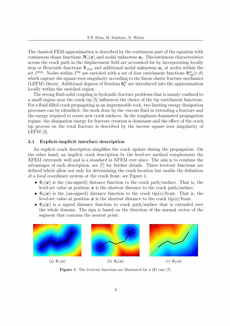
An explicit crack description simplifies the crack update during the propagation. Onthe other hand, an implicit crack description by the level-set method complements theXFEM extremely well and is a standard in XFEM ever since. The aim is to combine theadvantages of each description, see [7] for further details. Three level-set functions aredefined which allow not only for determining the crack location but enable the definitionof a local coordinate system at the crack front, see Figure 1.

• Φ1(x) is the (un-signed) distance function to the crack path/surface. That is, thelevel-set value at position x is the shortest distance to the crack path/surface.

• Φ2(x) is the (un-signed) distance function to the crack tip(s)/front. That is, thelevel-set value at position x is the shortest distance to the crack tip(s)/front.

• Φ3(x) is a signed distance function to crack path/surface that is extended overthe whole domain. The sign is based on the direction of the normal vector of thesegment that contains the nearest point.

(a) Φ1(x) (b) Φ2(x) (c) Φ3(x)

Figure 1: The level-set functions are illustrated for a 2D case [7].

4


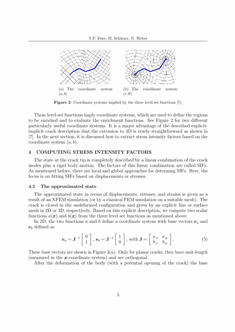
(a) The coordinate system(a, b)

(b) The coordinate system(r, θ)

Figure 2: Coordinate systems implied by the three level-set functions [7].

These level-set functions imply coordinate systems, which are used to define the regionsto be enriched and to evaluate the enrichment functions. See Figure 2 for two differentparticularly useful coordinate systems. It is a major advantage of the described explicit-implicit crack description that the extension to 3D is truely straightforward as shown in[7]. In the next section, it is discussed how to extract stress intensity factors based on thecoordinate system (a, b).

4 COMPUTING STRESS INTENSITY FACTORS

The state at the crack tip is completely described by a linear combination of the crackmodes plus a rigid body motion. The factors of this linear combination are called SIFs.As mentioned before, there are local and global approaches for determing SIFs. Here, thefocus is on fitting SIFs based on displacements or stresses.

4.1 The approximated state

The approximated state in terms of displacements, stresses, and strains is given as aresult of an XFEM simulation (or by a classical FEM simulation on a suitable mesh). Thecrack is closed in the undeformed configuration and given by an explicit line or surfacemesh in 2D or 3D, respectively. Based on this explicit description, we compute two scalarfunctions a(x) and b(x) from the three level set functions as mentioned above.

In 2D, the two functions a and b define a coordinate system with base vectors ea andeb defined as

ea = J−1

[01

]

, eb = J−1

[10

]

, with J =

[a,x a,yb,x b,y

]

. (5)

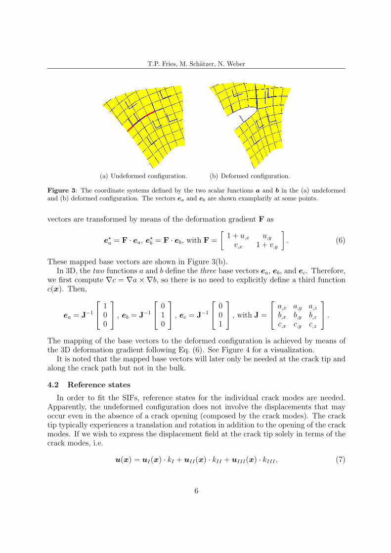
These base vectors are shown in Figure 3(a). Only for planar cracks, they have unit-length(measured in the x-coordinate system) and are orthogonal.

After the deformation of the body (with a potential opening of the crack) the base

5


(a) Undeformed configuration. (b) Deformed configuration.

Figure 3: The coordinate systems defined by the two scalar functions a and b in the (a) undeformedand (b) deformed configuration. The vectors ea and eb are shown examplarily at some points.

vectors are transformed by means of the deformation gradient F as

e⋆a = F · ea, e

⋆b = F · eb, with F =

[1 + u,x u,y

v,x 1 + v,y

]

. (6)

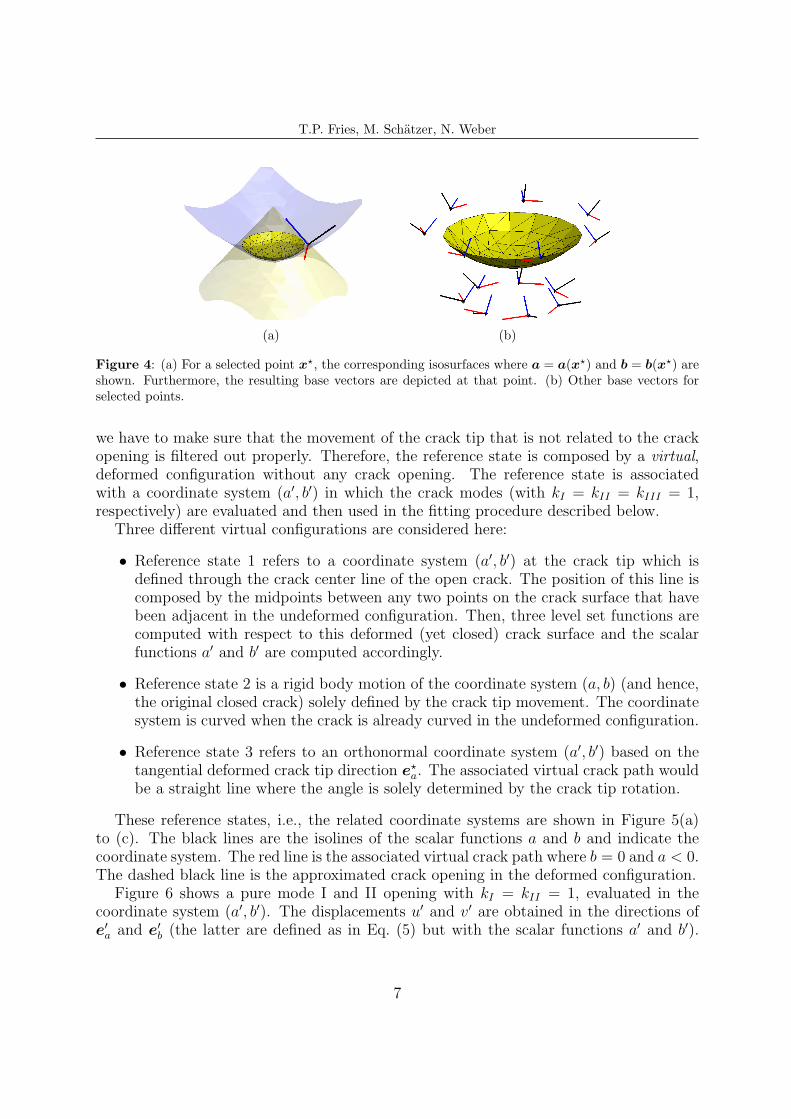
These mapped base vectors are shown in Figure 3(b).In 3D, the two functions a and b define the three base vectors ea, eb, and ec. Therefore,

we first compute ∇c = ∇a×∇b, so there is no need to explicitly define a third functionc(x). Then,

ea = J−1

100

, eb = J−1

010

, ec = J−1

001

, with J =

a,x a,y a,zb,x b,y b,zc,x c,y c,z

.

The mapping of the base vectors to the deformed configuration is achieved by means ofthe 3D deformation gradient following Eq. (6). See Figure 4 for a visualization.

It is noted that the mapped base vectors will later only be needed at the crack tip andalong the crack path but not in the bulk.

4.2 Reference states

In order to fit the SIFs, reference states for the individual crack modes are needed.Apparently, the undeformed configuration does not involve the displacements that mayoccur even in the absence of a crack opening (composed by the crack modes). The cracktip typically experiences a translation and rotation in addition to the opening of the crackmodes. If we wish to express the displacement field at the crack tip solely in terms of thecrack modes, i.e.

u(x) = uI(x) · kI + uII(x) · kII + uIII(x) · kIII , (7)

6


(a) (b)

Figure 4: (a) For a selected point x⋆, the corresponding isosurfaces where a = a(x⋆) and b = b(x⋆) areshown. Furthermore, the resulting base vectors are depicted at that point. (b) Other base vectors forselected points.

we have to make sure that the movement of the crack tip that is not related to the crackopening is filtered out properly. Therefore, the reference state is composed by a virtual,deformed configuration without any crack opening. The reference state is associatedwith a coordinate system (a′, b′) in which the crack modes (with kI = kII = kIII = 1,respectively) are evaluated and then used in the fitting procedure described below.

Three different virtual configurations are considered here:

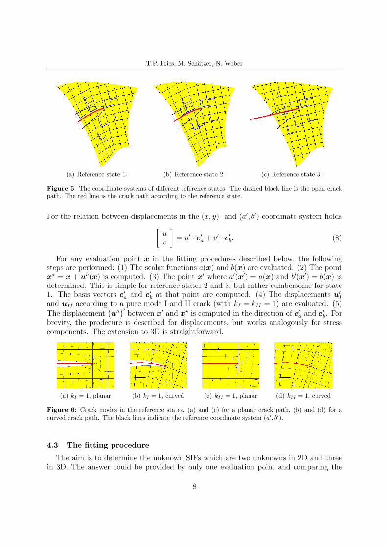
• Reference state 1 refers to a coordinate system (a′, b′) at the crack tip which isdefined through the crack center line of the open crack. The position of this line iscomposed by the midpoints between any two points on the crack surface that havebeen adjacent in the undeformed configuration. Then, three level set functions arecomputed with respect to this deformed (yet closed) crack surface and the scalarfunctions a′ and b′ are computed accordingly.

• Reference state 2 is a rigid body motion of the coordinate system (a, b) (and hence,the original closed crack) solely defined by the crack tip movement. The coordinatesystem is curved when the crack is already curved in the undeformed configuration.

• Reference state 3 refers to an orthonormal coordinate system (a′, b′) based on thetangential deformed crack tip direction e⋆

a. The associated virtual crack path wouldbe a straight line where the angle is solely determined by the crack tip rotation.

These reference states, i.e., the related coordinate systems are shown in Figure 5(a)to (c). The black lines are the isolines of the scalar functions a and b and indicate thecoordinate system. The red line is the associated virtual crack path where b = 0 and a < 0.The dashed black line is the approximated crack opening in the deformed configuration.

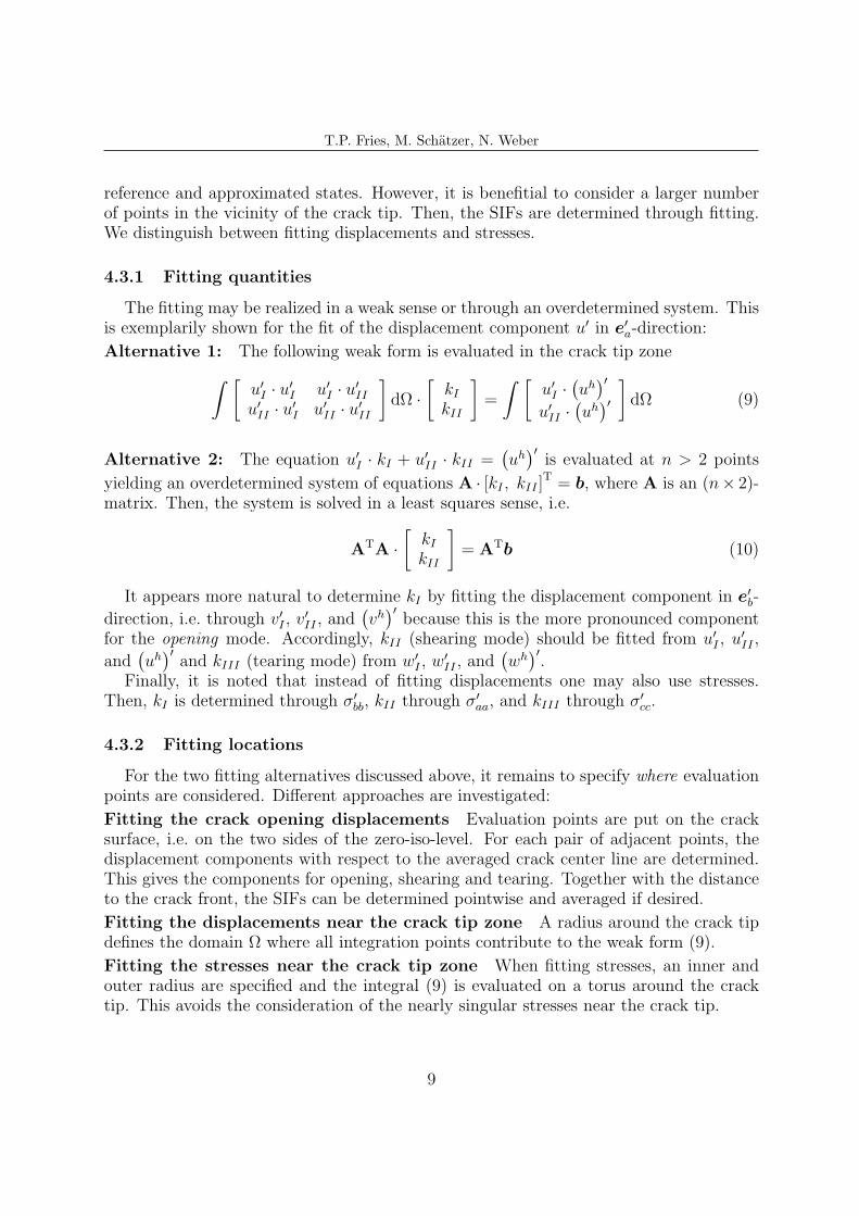
Figure 6 shows a pure mode I and II opening with kI = kII = 1, evaluated in thecoordinate system (a′, b′). The displacements u′ and v′ are obtained in the directions ofe′

a and e′

b (the latter are defined as in Eq. (5) but with the scalar functions a′ and b′).

7


(a) Reference state 1. (b) Reference state 2. (c) Reference state 3.

Figure 5: The coordinate systems of different reference states. The dashed black line is the open crackpath. The red line is the crack path according to the reference state.

For the relation between displacements in the (x, y)- and (a′, b′)-coordinate system holds

[uv

]

= u′· e′

a + v′ · e′

b. (8)

For any evaluation point x in the fitting procedures described below, the followingsteps are performed: (1) The scalar functions a(x) and b(x) are evaluated. (2) The pointx⋆ = x + uh(x) is computed. (3) The point x′ where a′(x′) = a(x) and b′(x′) = b(x) isdetermined. This is simple for reference states 2 and 3, but rather cumbersome for state1. The basis vectors e′

a and e′

b at that point are computed. (4) The displacements u′

I

and u′

II according to a pure mode I and II crack (with kI = kII = 1) are evaluated. (5)

The displacement(uh)′

between x′ and x⋆ is computed in the direction of e′

a and e′

b. Forbrevity, the prodecure is described for displacements, but works analogously for stresscomponents. The extension to 3D is straightforward.

(a) kI = 1, planar (b) kI = 1, curved (c) kII = 1, planar (d) kII = 1, curved

Figure 6: Crack modes in the reference states, (a) and (c) for a planar crack path, (b) and (d) for acurved crack path. The black lines indicate the reference coordinate system (a′, b′).

4.3 The fitting procedure

The aim is to determine the unknown SIFs which are two unknowns in 2D and threein 3D. The answer could be provided by only one evaluation point and comparing the

8


reference and approximated states. However, it is benefitial to consider a larger numberof points in the vicinity of the crack tip. Then, the SIFs are determined through fitting.We distinguish between fitting displacements and stresses.

4.3.1 Fitting quantities

The fitting may be realized in a weak sense or through an overdetermined system. Thisis exemplarily shown for the fit of the displacement component u′ in e′

a-direction:

Alternative 1: The following weak form is evaluated in the crack tip zone

∫ [u′

I · u′

I u′

I · u′

II

u′

II · u′

I u′

II · u′

II

]

dΩ ·

[kIkII

]

=

∫ [u′

I ·(uh)′

u′

II ·(uh)′

]

dΩ (9)

Alternative 2: The equation u′

I · kI + u′

II · kII =(uh)′

is evaluated at n > 2 points

yielding an overdetermined system of equations A · [kI , kII ]T = b, where A is an (n× 2)-

matrix. Then, the system is solved in a least squares sense, i.e.

ATA ·

[kIkII

]

= ATb (10)

It appears more natural to determine kI by fitting the displacement component in e′

b-

direction, i.e. through v′I , v′

II , and(vh)′

because this is the more pronounced componentfor the opening mode. Accordingly, kII (shearing mode) should be fitted from u′

I , u′

II ,

and(uh)′

and kIII (tearing mode) from w′

I , w′

II , and(wh)′

.Finally, it is noted that instead of fitting displacements one may also use stresses.

Then, kI is determined through σ′

bb, kII through σ′

aa, and kIII through σ′

cc.

4.3.2 Fitting locations

For the two fitting alternatives discussed above, it remains to specify where evaluationpoints are considered. Different approaches are investigated:

Fitting the crack opening displacements Evaluation points are put on the cracksurface, i.e. on the two sides of the zero-iso-level. For each pair of adjacent points, thedisplacement components with respect to the averaged crack center line are determined.This gives the components for opening, shearing and tearing. Together with the distanceto the crack front, the SIFs can be determined pointwise and averaged if desired.

Fitting the displacements near the crack tip zone A radius around the crack tipdefines the domain Ω where all integration points contribute to the weak form (9).

Fitting the stresses near the crack tip zone When fitting stresses, an inner andouter radius are specified and the integral (9) is evaluated on a torus around the cracktip. This avoids the consideration of the nearly singular stresses near the crack tip.

9


Fitting the displacements on circles Instead of evaluating an integral in the bulk,one may also define a circle around the crack tip and place evaluation points on the circle.Then, we solve (10) in order to fit displacements.

Fitting the stresses on circles Again, evaluation points on a circle with a prescribedradius are placed around the crack tip. Then, the SIFs are obtained by fitting the stresscompenent σ′

rθ in a polar coordinate system. The polar coordinates are easily obtainedfrom the (a′, b′)-coordinate system. The advantage of this approach is that only an arc ofthe circle in front of the crack tip can be considered. In that region, the three referencestates coincide.

5 NUMERICAL RESULTS

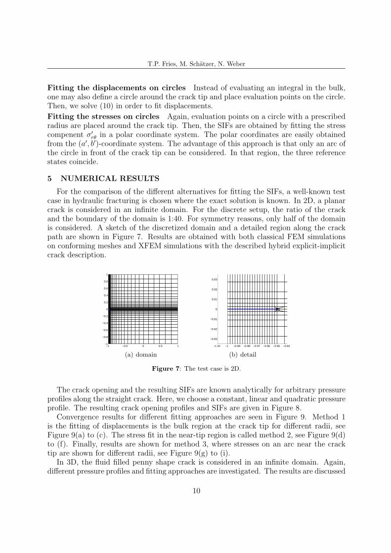
For the comparison of the different alternatives for fitting the SIFs, a well-known testcase in hydraulic fracturing is chosen where the exact solution is known. In 2D, a planarcrack is considered in an infinite domain. For the discrete setup, the ratio of the crackand the boundary of the domain is 1:40. For symmetry reasons, only half of the domainis considered. A sketch of the discretized domain and a detailed region along the crackpath are shown in Figure 7. Results are obtained with both classical FEM simulationson conforming meshes and XFEM simulations with the described hybrid explicit-implicitcrack description.

−1 −0.5 0 0.5 1−1

−0.8

−0.6

−0.4

−0.2

0

0.2

0.4

0.6

0.8

1

(a) domain

−1.01 −1 −0.99 −0.98 −0.97 −0.96 −0.95 −0.94

−0.03

−0.02

−0.01

0

0.01

0.02

0.03

(b) detail

Figure 7: The test case is 2D.

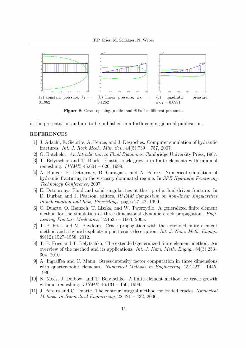
The crack opening and the resulting SIFs are known analytically for arbitrary pressureprofiles along the straight crack. Here, we choose a constant, linear and quadratic pressureprofile. The resulting crack opening profiles and SIFs are given in Figure 8.

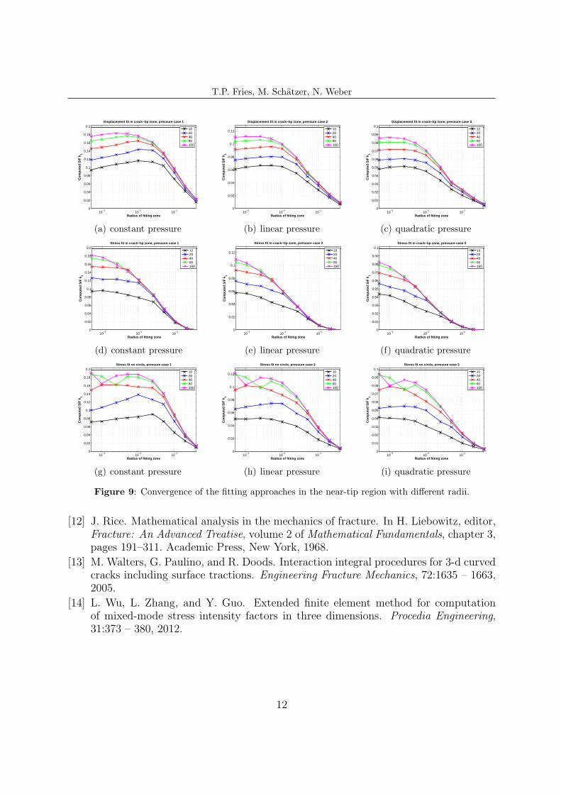
Convergence results for different fitting approaches are seen in Figure 9. Method 1is the fitting of displacements is the bulk region at the crack tip for different radii, seeFigure 9(a) to (c). The stress fit in the near-tip region is called method 2, see Figure 9(d)to (f). Finally, results are shown for method 3, where stresses on an arc near the cracktip are shown for different radii, see Figure 9(g) to (i).

In 3D, the fluid filled penny shape crack is considered in an infinite domain. Again,different pressure profiles and fitting approaches are investigated. The results are discussed

10


−1 −0.99 −0.98 −0.97 −0.96 −0.95−5

−4

−3

−2

−1

0

1

2

3

4

5x 10

−3

p0=0.50

(a) constant pressure, kI =0.1982

−1 −0.99 −0.98 −0.97 −0.96 −0.95−5

−4

−3

−2

−1

0

1

2

3

4

5x 10

−3

p0=0.50

(b) linear pressure, kII =0.1262

−1 −0.99 −0.98 −0.97 −0.96 −0.95−5

−4

−3

−2

−1

0

1

2

3

4

5x 10

−3

p0=0.50

(c) quadratic pressure,kIII = 0.0991

Figure 8: Crack opening profiles and SIFs for different pressures.

in the presentation and are to be published in a forth-coming journal publication.

REFERENCES

[1] J. Adachi, E. Siebrits, A. Peirce, and J. Desroches. Computer simulation of hydraulicfractures. Int. J. Rock Mech. Min. Sci., 44(5):739 – 757, 2007.

[2] G. Batchelor. An Introduction to Fluid Dynamics. Cambridge University Press, 1967.

[3] T. Belytschko and T. Black. Elastic crack growth in finite elements with minimalremeshing. IJNME, 45:601 – 620, 1999.

[4] A. Bunger, E. Detournay, D. Garagash, and A. Peirce. Numerical simulation ofhydraulic fracturing in the viscosity dominated regime. In SPE Hydraulic Fracturing

Technology Conference, 2007.

[5] E. Detournay. Fluid and solid singularities at the tip of a fluid-driven fracture. InD. Durban and J. Pearson, editors, IUTAM Symposium on non-linear singularities

in deformation and flow, Proceedings, pages 27–42, 1999.

[6] C. Duarte, O. Hamzeh, T. Liszka, and W. Tworzydlo. A generalized finite elementmethod for the simulation of three-dimensional dynamic crack propagation. Engi-

neering Fracture Mechanics, 72:1635 – 1663, 2005.

[7] T.-P. Fries and M. Baydoun. Crack propagation with the extended finite elementmethod and a hybrid explicit–implicit crack description. Int. J. Num. Meth. Engng.,89(12):1527–1558, 2012.

[8] T.-P. Fries and T. Belytschko. The extended/generalized finite element method: Anoverview of the method and its applications. Int. J. Num. Meth. Engng., 84(3):253–304, 2010.

[9] A. Ingraffea and C. Manu. Stress-intensity factor computation in three dimensionswith quarter-point elements. Numerical Methods in Engineering, 15:1427 – 1445,1980.

[10] N. Moes, J. Dolbow, and T. Belytschko. A finite element method for crack growthwithout remeshing. IJNME, 46:131 – 150, 1999.

[11] J. Pereira and C. Duarte. The contour integral method for loaded cracks. Numerical

Methods in Biomedical Engineering, 22:421 – 432, 2006.

11


10−3

10−2

10−1

0

0.02

0.04

0.06

0.08

0.1

0.12

0.14

0.16

0.18

0.2

Radius of fitting zone

Com

pute

d S

IF k

1

Displacement fit in crack−tip zone, pressure case 1

10204080160

(a) constant pressure

10−3

10−2

10−1

0

0.02

0.04

0.06

0.08

0.1

0.12


Com

pute

d S

IF k

1


10204080160

(b) linear pressure

10−3

10−2

10−1

0

0.01

0.02

0.03

0.04

0.05

0.06

0.07

0.08

0.09

0.1


Com

pute

d S

IF k

1


10204080160

(c) quadratic pressure

10−3

10−2

10−1

0

0.02

0.04

0.06

0.08

0.1

0.12

0.14

0.16

0.18

0.2


Com

pute

d S

IF k

1

Stress fit in crack−tip zone, pressure case 1

10204080160

(d) constant pressure

10−3

10−2

10−1

0

0.02

0.04

0.06

0.08

0.1

0.12


Com

pute

d S

IF k

1


10204080160

(e) linear pressure

10−3

10−2

10−1

0

0.01

0.02

0.03

0.04

0.05

0.06

0.07

0.08

0.09

0.1


Com

pute

d S

IF k

1


10204080160

(f) quadratic pressure

10−3

10−2

10−1

0

0.02

0.04

0.06

0.08

0.1

0.12

0.14

0.16

0.18

0.2


Com

pute

d S

IF k

1

Stress fit on circle, pressure case 1

10204080160

(g) constant pressure

10−3

10−2

10−1

0

0.02

0.04

0.06

0.08

0.1

0.12


Com

pute

d S

IF k

1


10204080160

(h) linear pressure

10−3

10−2

10−1

0

0.01

0.02

0.03

0.04

0.05

0.06

0.07

0.08

0.09

0.1


Com

pute

d S

IF k

1


10204080160

(i) quadratic pressure

Figure 9: Convergence of the fitting approaches in the near-tip region with different radii.

[12] J. Rice. Mathematical analysis in the mechanics of fracture. In H. Liebowitz, editor,Fracture: An Advanced Treatise, volume 2 of Mathematical Fundamentals, chapter 3,pages 191–311. Academic Press, New York, 1968.

[13] M. Walters, G. Paulino, and R. Doods. Interaction integral procedures for 3-d curvedcracks including surface tractions. Engineering Fracture Mechanics, 72:1635 – 1663,2005.

[14] L. Wu, L. Zhang, and Y. Guo. Extended finite element method for computationof mixed-mode stress intensity factors in three dimensions. Procedia Engineering,31:373 – 380, 2012.

12

Documents

XFEM-SIMULATION OF HYDRAULIC FRACTURING IN 3D WITH