Copyright 2015, AADE

This paper was prepared for presentation at the 2015 AADE National Technical Conference and Exhibition held at the Henry B. Gonzalez Convention Center, San Antonio, Texas, April 8-9, 2015. This conference was sponsored by the American Association of Drilling Engineers. The information presented in this paper does not reflect any position, claim or endorsement made or implied by the American

Association of Drilling Engineers, their officers or members. Questions concerning the content of this paper should be directed to the individual(s) listed as author(s) of this work.

Abstract The Cohesive Zone Model (CZM) honors the fracture tip

effects in a quasi-brittle rock such as shale, which results in a

more precise fracture geometry and pumping pressure

compared to those from Linear Elastic Fracture Mechanics.

Nevertheless, this model, namely planar CZM, assumes a

predefined surface on which the fractures propagate and

therefore, restricts the fracture propagation direction. Notably,

this direction can be acquired integrating CZM as the segmental

contact interaction model with a fully coupled pore pressure-

displacement, extended finite element model (XFEM).

In this work, we modeled triple-stage 3D hydraulic

fracturing in a single-layer, quasi-brittle shale formation using

planar CZM and XFEM-based CZM including slit flow and

poro-elasticity for fracture and matrix spaces, respectively, in

Abaqus. Our fully-coupled pore pressure-stress Geo-mechanics

model includes leak-off as a continuum-based fluid flow

component coupled with the other unknowns in the problem.

Having compared the triple-stage fracturing results from

planar CZM with those from XFEM-based CZM, we found that

the stress shadowing effect of hydraulic fractures on each other

can cause these fractures to rationally propagate out of plane.

We investigated the effect of this arbitrary propagation

direction on not only the fractures’ length, aperture, and the

required injection pressure, but also fractures’ connection to the

wellbore. Depending on the spacing, this connection can be

disrupted due to the near-wellbore fracture closure which may

embed proppant grains on the fracture wall, or screen out the

fracture at early times.

Introduction Shale gas resources have profoundly contributed to the

prospective independence of the U.S. on oil and gas from

foreign resources. The abundant condensate gas production and

export from the U.S. shale resources have significantly

contributed in the global sharp oil price decline since August

2014.1 These resources are constituted of ultra-low permeable,

organic-rich formations with desorption of gas as a major but

slow-rate and long-lasting producing mechanism. Economic

production from these resources through gas desorption

requires a complex network of natural fractures connected to

the producing horizontal wellbores by hydraulic fractures in

multiple stages, the most common stimulation technology in

shale gas reservoirs. The geometry of hydraulic fractures

(length, height, aperture, and propagation pattern) significantly

contributes to long-term gas production and is inspected

roughly by post-fracturing data acquisition methods such as

tiltmeter fracturing mapping and micro-seismic monitoring.2

This later method, however, cannot identify opening-mode or

hydraulic fractures since the only detectable events using this

method are shear slippage events. The technical restrictions on

the hydraulic fracture data acquisition, the limitation on the

extendibility of a successful fracturing job data to the other

fields3, and the high cost of re-stimulation plans, if possible,

urge to develop numerical tools for optimal hydraulic fracturing

design. Furthermore, due to the occurrence of cap rock and

shale gas reservoir in close proximity and the environmental

concerns about ground water contamination by fracking jobs,

the induced fractures need to be cautiously placed in order not

to propagate into the upper and lower geological layers. Such a

rigorous hydraulic fracture design in shale rocks demands

numerical optimizing tools which should also be versatile for a

variety of shale formations in mineralogy and stress state and

capture increasingly more complex fracture networks than

expected in these resources .2,4

Hydraulic fracturing is defined as a fully coupled porous

solid-fluid interaction problem where the fracturing force, the

fluid pressure on the fracture walls, exceeds the minimum in

situ principal stress plus the tensile strength of the rock.5 The

coupled phenomena include the fracturing fluid flow within the

fracture, the fluid flow in the surrounding porous media, the

permeation (leak-off) of the fracturing fluid into the formation ,

the matrix mechanical deformation, and the fracture growth.6

Fluid leak-off and spurt loss depend on the fracturing fluid

pressure, more fluid bleed-off leads to more pressure drop along

fracture and less fracture propagation, and rock deformation

alters the matrix porosity and permeability and therefore the

fluid flow in the surrounding porous media. The hydraulic

fractures potentially open and close (hysteresis effect) due to

fracturing pressure alteration7 which can be a consequence of

AADE-15-NTCE-28

Integration of XFEM and CZM to Model 3D Multiple-Stage Hydraulic Fracturing in Quasi-brittle Shale Formations: Solution-Dependent Propagation Direction Mahdi Haddad and Kamy Sepehrnoori, The University of Texas at Austin

2 M. Haddad and K. Sepehrnoori AADE-15-NTCE-28

step-wise or unstable fracture propagation.8,9 Furthermore, the

more complexity in the hydraulic fracture patterns is partially

attributed to stress shadows of pre-existing or simultaneously

growing fractures9,10, or the residual stresses from the previous

completion operations11. These physical complexities challenge

the majority of the existing models which are based on Linear

Elastic Fracture Mechanics (LEFM), and restricted to linear

rock failure and single-stage planar fracture propagation such

as planar 3D (PL3D) models based on boundary integral

method12.

The simulation of hydraulic fracturing has been conducted

by a variety of numerical methods such as Boundary Element

Method (BEM) also called displacement discontinuity method

or boundary integral method13,14, and Finite Element Method

(FEM)15. BEM cannot rigorously take into account the material

heterogeneities and requires re-meshing during fracture

propagation16 whereas the classical FEM restricts the fracture

path to the element edges15,17 or along a pre-defined path named

cohesive layer10. Nonetheless, the adoption of Cohesive Zone

Model (CZM) in FEM enables to include the material softening

effects at the fracture tip process zone, which simulates the

quasi-brittle fracture propagation in shale rocks compared to

ductile and brittle fracture propagation in steel and glass,

respectively18. Furthermore, despite the common perception

about the restriction of CZM in modeling non-intersecting

fractures, Gonzalez and Dahi19 investigated intersecting

hydraulic and natural fractures simply by modifying the

cohesive elements’ middle nodes at the intersection.

In contrast to the classical FEM, the eXtended Finite

Element Method (XFEM) can simulate the fracture propagation

along arbitrary paths independent of the mesh. Lately, this

method has been extended in Abaqus for the simulation of

hydraulic fracturing by adding “edge” phantom nodes with pore

pressure degree of freedom besides the previously developed

“corner” phantom nodes 20,21; we call this method as XFEM -

based CZM. Compared to the most commercial hydraulic

fracturing simulators in the upstream oil and gas industry12 or

even the recently developed models22, the new capability

provides the following improvements: 1) more plausible model

for quasi-brittle rocks; 2) fully coupled pore pressure/stress

analysis for the matrix and arbitrarily propagating fracture; 3)

leak-off model based on fluid continuity and coupled with

matrix deformation; 4) ability to include reservoir

heterogeneities; and 5) fracturing simulation under the

disturbed stress state due to the previous completion steps.

The theme of the current work is to apply the recently

developed XFEM-based CZM in Abaqus for the simulation of

simultaneous triple-stage hydraulic fracturing at various

spacing and compare the results with those from the

conventional CZM with pre-defined planar cohesive layers. We

narrow our investigation down to the simultaneous fracturing

scenarios after the work done by Haddad and Sepehrnoori10

who demonstrated the superiority of the simultaneous

fracturing scenario to achieve the best fracture geometries. This

work includes additional geometric and physical characteristics

such as non-planar fracture propagation, stress interactions

between hydraulic fractures, and onset of the coalescence or

divergence of fractures.

Method

In order to avoid re-meshing during the hydraulic fracturing

simulation, and to improve the fracture tip solutions, a mesh

independent crack growth model, XFEM, was proposed in the

works done by Belytschko and Black23 and Moes et al.24.

Compared to the other FEM-based crack simulation methods,

XFEM demonstrates several advantages such as the following :

1) arbitrary fracture growth direction predicted based on the

current stress state close to the fracture tip; 2) easier initial crack

definition; 3) simpler mesh refinement studies; 4) improved

convergence rates in the case of stationary cracks; and 4)

application in general static and implicit dynamic procedures20.

XFEM incorporates the discontinuous geometry, the fracture,

and the discontinuous field by enriching the finite element basis

functions, Eq. (1), after Belytschko and Black23 based on the

partition of unity method of Babuska and Melenk25. The

enrichment functions must be selected based on the class of

problems, which includes a priori knowledge of partial

differential equation behavior into finite element space

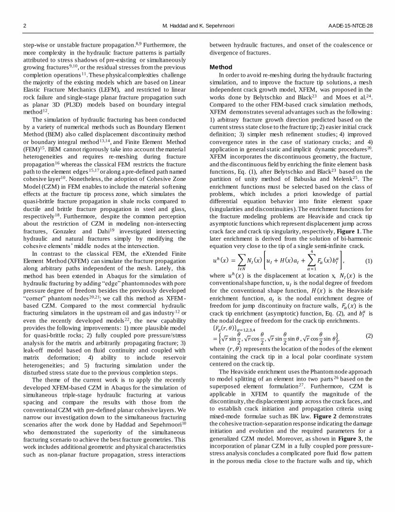
(singularities and discontinuities). The enrichment functions for

the fracture modeling problems are Heaviside and crack tip

asymptotic functions which represent displacement jump across

crack face and crack tip singularity, respectively, Figure 1. The

later enrichment is derived from the solution of bi-harmonic

equation very close to the tip of a single semi-infinite crack.

𝑢ℎ (𝑥) = ∑ 𝑁𝐼(𝑥) [𝑢𝐼 + 𝐻(𝑥)𝑎𝐼 + ∑ 𝐹𝛼

(𝑥)𝑏𝐼𝛼

4

𝛼 =1

] ,𝐼𝜖𝑁

(1)

where 𝑢ℎ (𝑥) is the displacement at location x, 𝑁𝐼 (𝑥) is the

conventional shape function, 𝑢𝐼 is the nodal degree of freedom

for the conventional shape function, 𝐻 (𝑥) is the Heaviside

enrichment function, 𝑎𝐼 is the nodal enrichment degree of

freedom for jump discontinuity on fracture walls, 𝐹𝛼(𝑥) is the

crack tip enrichment (asymptotic) function, Eq. (2), and 𝑏𝐼𝛼 is

the nodal degree of freedom for the crack tip enrichments. {𝐹𝛼(𝑟, 𝜃)}𝛼=1,2,3,4

= {√𝑟 sin𝜃

2, √𝑟cos

𝜃

2, √𝑟 sin

𝜃

2sin 𝜃 , √𝑟 cos

𝜃

2sin 𝜃},

(2)

where (𝑟, 𝜃) represents the location of the nodes of the element

containing the crack tip in a local polar coordinate system

centered on the crack tip.

The Heaviside enrichment uses the Phantom node approach

to model splitting of an element into two parts 26 based on the

superposed element formulation27. Furthermore, CZM is

applicable in XFEM to quantify the magnitude of the

discontinuity, the displacement jump across the crack faces, and

to establish crack initiation and propagation criteria using

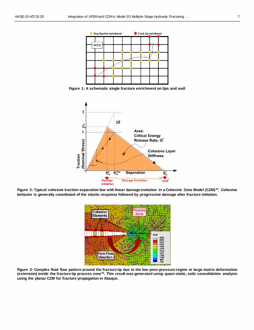
mixed-mode formulae such as BK law. Figure 2 demonstrates

the cohesive traction-separation response indicating the damage

initiation and evolution and the required parameters for a

generalized CZM model. Moreover, as shown in Figure 3, the

incorporation of planar CZM in a fully coupled pore pressure-

stress analysis concludes a complicated pore fluid flow pattern

in the porous media close to the fracture walls and tip, which

AADE-15-NTCE-28 Integration of XFEM and CZM to Model 3D Multiple-Stage Hydraulic Fracturing … 3

disapproves the application of Carter’s linear, 1D leak-off

model28.

Nevertheless, the cohesive response in XFEM-based CZM

does not include the elastic part in Figure 2 and the cohesive

layer undergoes progressive damage at zero separation when

the fracture initiation criterion is satisfied, Figure 4. Notably,

the elastic response is inherently included in the elastic

deformation of the porous media ahead of the fracture tip before

further fracture propagation.

Furthermore, in XFEM, a method is required to locate the

discontinuity; for instance, level set method (LSM). A level set

of a real-valued function is the set of all points at which the

function attains a specified value. This method is a popular

technique for representing surfaces in interface tracking

problems since for instance, XFEM cracks require the value of

this function only at nodes belonging to elements cut by the

crack. Generally, two functions Φ and Ψ are used for a

complete description of crack faces and tips. However, only one

level set function,Φ is sufficient to locate a crack if the crack

propagates always up to the element edges. Using LSM in

XFEM eases the calculation of contour integrals compared to

traditional mesh-dependent methods since the level set

functions’ values at the nodes in an element automatically

provide the required data for the contour integral.

XFEM must be cautiously applied for the simulation of

fracturing in Abaqus due to the following29: 1) it requires very

fine mesh close to the fracture propagation region to predict the

correct growth direction; 2) the enrichment zone should exclude

the “hotspots” such as boundaries or the other modeling

artifacts in order to avoid unrealistic fracture propagations; 3)

the phantom nodes on the boundaries must be constrained; and

4) the initial fractures (perforations) should cross fewer

elements for the fast convergence of the solution at early times.

Model Construction

Hydraulic fracturing simulation using XFEM-based CZM is

computationally more expensive than that using planar CZM as

the reasonable convergence of the solution during fracture

deviation in XFEM requires a very fine mesh in a large

enrichment zone whereas the pre-defined fracture path in planar

CZM needs refined mesh very close to the cohesive layer(s).

Due to the restrictions in dynamic mesh refinement during

XFEM analysis in Abaqus and the computational limits on the

number of elements, we modeled hydraulic fracturing in a 3D

geometry using a single layer of adequately fine mesh using 3D

solid elements with pore pressure degree of freedom, C3D8P.

Thus, the current work limits height growth to a single layer of

elements; notably, our implemented XFEM-based CZM

method is capable of simulating fully 3D hydraulic fracturing

with higher computational expenses. Moreover, the solution

from this model configuration can be simply verified

comparing that with the analytical solution by Geertsma and de

Klerk30. Due to the advantages of simultaneous hydraulic

fracturing compared to sequential one10, we restricted our

investigation to a simultaneous fracturing scenario with three

fractures (clusters) per stage, Figure 5. We defined one

enrichment zone per fracture with the variable enrichment zone

size; the middle fracture supposedly propagates straight, which

requires a thin enrichment zone, Enrichment Zone 2. For better

mesh size transition, we used the sweep meshing technique with

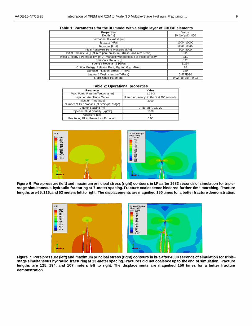
advancing front20. The input parameters of the model can be

found in Tables 1 and 2. We discretely perturbed some default

values in order to investigate the effect of various parameters in

our fully coupled poro-elastic solution, and also approach the

real field data.

Results and Discussion

Figures 6 through 8 demonstrate the fracture propagation

results for 7-, 13-, and 20-meter spacing, respectively.

According to these figures, fracture spacing can influence

fracture propagation in a variety of patterns from fracture

coalescence to divergence. At 7-meter spacing (Figure 6), the

side fractures propagate slightly toward the left and right

boundaries at early times while they coalesce the middle

fracture after 1683 seconds of simulation. In this solution,

fracture propagation is restricted to an exclusive enrichment

zone, which hurdles the physical coalescence of multiple

fractures; however, the implemented model predicts the

eminent proximity of fracture coalescence provided that the

thickness of the enrichment zones is selected cautiously. The

right contours in Figures 6 through 8 show the maximu m

principal stress to better demonstrate the stress shadowing

effect of fractures on each other, which better explains the

fracture propagation pattern.

Furthermore, the propagation of the side fractures in 7-

meter (Figure 6) and 13-meter (Figure 7) spacing closes the

middle fracture at the injection point, which may crush the

proppant grains, embed them on the fracture walls, or transport

them with the bulk of the fracturing fluid toward the fracture

tip; all these effects adversely influence the gas productivity of

the middle fracture. The same phenomenon can be observed in

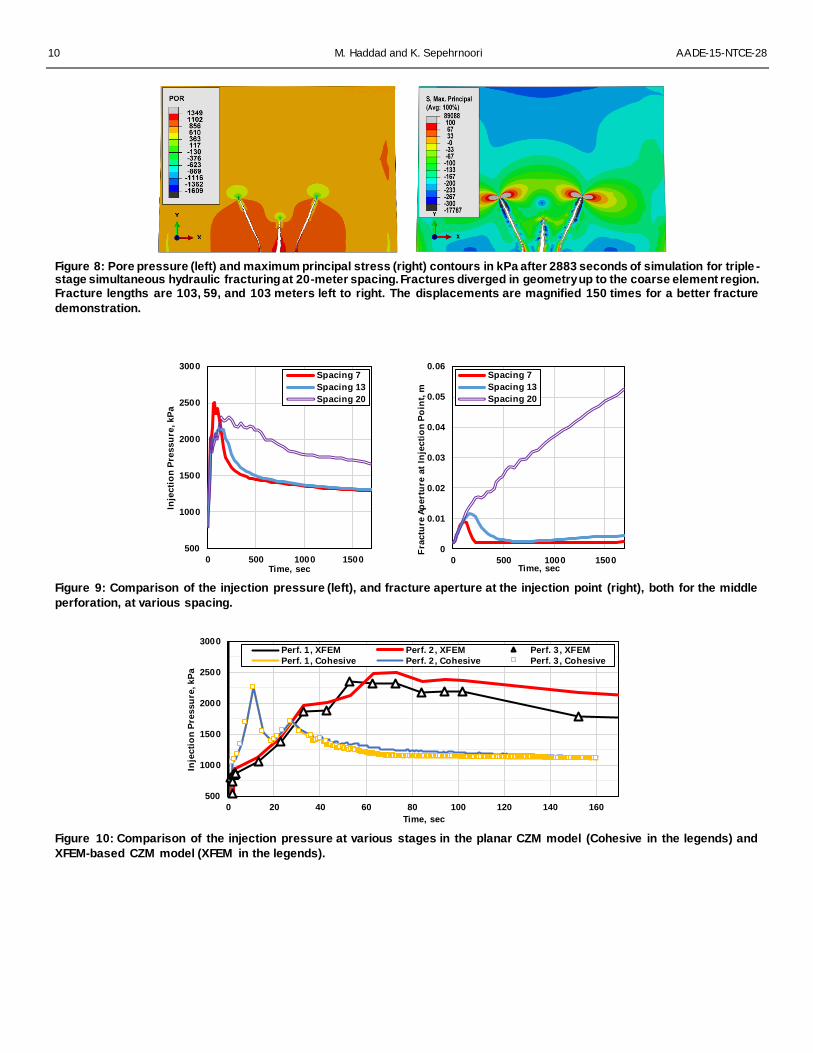
the case with 20-meter spacing, Figure 8, where the side

fractures close up at the injection points due to the growth of

the middle fracture. Moreover, the further propagation of the

side fractures in 20-meter spacing causes a compressional

region right ahead of the middle fracture (the circular, small

blue region ahead of the middle fracture tip in the right picture

of Figure 8), which prevents the middle fracture to grow as long

as the other fractures.

Moreover, the fractures in 13-meter spacing remain almost

parallel up to the end of the simulation whereas the middle

fracture grows longer than the others. This special configuration

causes the proximity of a high fluid pressure zone, within the

middle fracture, and the low pore pressure zones around the left

and right fracture tips, which concludes the fluid

communication between the side fractures and the middle

fracture. This fluid communication can be correlated to the

tensile maximum principal stress zones between the side

fracture tips and the middle fracture considering more severe

fluid leak-off from the middle fracture toward the side fractures,

Figure 7. As stated before, our fully coupled pore pressure-

stress analysis using XFEM-based CZM can provide rigorous

solutions for the complex physics around the fracture tips

including the nonlinear fluid flow patterns around fractures .

4 M. Haddad and K. Sepehrnoori AADE-15-NTCE-28

Figure 9 compares the injection pressure and fracture

aperture at the injection point for the middle perforation. The

results for 20-meter spacing follow different trends from those

for the other spacing values; this is consistent with the middle

fracture configuration, Figure 8, as the middle fracture at 20-

meter spacing grows shorter in length and therefore, expands

more in aperture, which leads to a wider aperture at the injection

point. As stated before, the compressional region ahead of the

middle fracture resists further propagation of the middle

fracture, which significantly contributes in the high injection

pressure and fracture aperture at the injection point for the

middle fracture.

Comparison of XFEM-based CZM and Planar CZM Our triple-stage hydraulic fracturing problem can be solved

also using planar CZM with the cohesive layers on three pre-

defined planes. All mechanical properties are the same as

before expect the following: 1) fracture initiation criterion,

which must be switched to quadratic nominal stress, QUADS,

as the maximum principal stress criterion, MAXPS, does not

lead to any fracture propagation on the cohesive layers; 2)

cohesive layer stiffness, which is 65 times that of the adjoining

material in planar CZM, and un-defined in XFEM-based CZM,

Figure 4.

Figures 10 and 11 respectively demonstrate the injection

pressure and fracture aperture at the injection point for various

stages using planar and XFEM-based CZM models. Both

models conclude the same general trend for the studied

parameters whereas the XFEM-based CZM predicts higher

values for these parameters compared to those from the planar

CZM.

As shown in Abaqus Benchmarks Guide31 for the

propagation of hydraulically driven fracture using XFEM, the

solution from XFEM-based CZM is highly sensitive to mesh

refinement such that an extremely fine mesh can conclude an

XFEM solution very close to the planar CZM solution.

Nonetheless, the investigated problem in the above reference is

a single-stage 2D hydraulic fracturing problem with a known

propagation path which restricts mesh refinement to a narrow

region around itself. However, in a multi-stage hydraulic

fracturing problem, the mesh refinement region cannot be

restricted to a small area as fractures can propagate on arbitrary

paths due to the stress shadowing effect and mesh refinement in

a big region is required, Figure 8. Therefore, even with a very

fine mesh, we could not prove mesh independency of the

solution for injection pressure, Figure 10.

Furthermore, the planar CZM results in a lower fracture

aperture at the injection point compared to that from the XFEM-

based CZM, Figure 11. This trend can be attributed to the

following issues: 1) inadequate mesh refinement around the

fractures; and 2) the restriction of the fractures to propagate on

pre-defined paths in the planar CZM in contrast to the freedom

of the fractures to propagate on arbitrary paths in the XFEM -

based CZM.

Parametric Study The above results were drawn at low horizontal stresses and

low stress contrast (the difference between minimum and

maximum horizontal stresses), which concluded long fracture

propagation and high deviations. In order to demonstrate the

effect of the stress contrast and absolute values of the stresses

on fracture deviation, we investigated fracture propagation at 7-

meter spacing for a range of maximum horizontal stresses,

keeping the minimum horizontal stress constant, and

amplifying pore pressure and stresses 10 times those in the

previous results or Table 1. This stress amplification shifts input

data toward more realistic field values. As observed in Figure

12, higher absolute values for stresses and pore pressure

conclude lower fracture deviation meaning that the fractures

intend to grow longer without coalescence or divergence.

Moreover, increasing the stress contrast or the maximu m

horizontal stress leads to less deviation of the side fractures and

the middle fracture closure, which agrees with the middle

fracture configuration at low stresses, Figure 6. Therefore,

fracture propagation and deviation highly depends on the

maximum horizontal stress or stress contrast, and the absolute

values of the stresses.

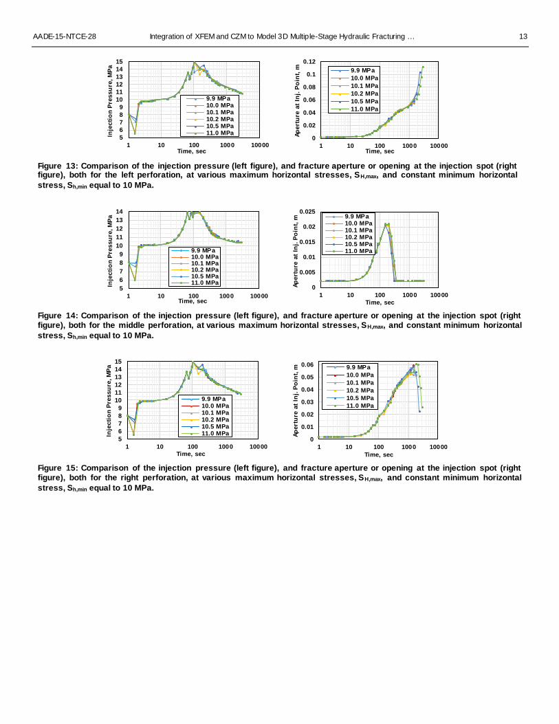
In order to quantify the effect of the stress contrast on the

properties of hydraulic fractures, we compared the injection

pressure and fracture aperture at the injection point for left,

middle, and right perforations in Figures 13, 14, and 15,

respectively. These figures show that the maximum horizontal

stress negligible effects the injection pressure and fracture

aperture at the injection point for various perforations.

Nevertheless, a variation in the injection pressure can be

observed for different maximum horizontal stresses around 150

seconds of injection, which can originate from the nonplanar

fracture propagation and the stress interaction of fractures with

each other.

Figures 13 and 15 demonstrate consistent left and right

fracture closure at the injection point as the opening of the left

fracture coincides with the closure of the right fracture after

1000 seconds of injection. Moreover, Figure 14 shows that the

middle fracture closes up to 2 millimeters, the fracture aperture

at early times, after 300 seconds of injection, which

demonstrates the negligible contribution of the middle fracture

in production.

Conclusions

Using a fully coupled pore pressure-stress, quasi-static,

finite strain analysis, we solved 3D triple-stage hydraulic

fracturing problems. The fractures were modeled using CZM

and XFEM-based CZM; the first model is advantageous with

respect to LEFM for quasibrittle rocks such as shales due to a

more rigorous treatment with the process zones ahead of the

fracture tips. In addition to this advantage, the second model

releases the restriction on the fracture propagation plan in CZM.

Mechanical interactions or stress shadowing effects of closely

spaced hydraulic fractures concluded the following remarks:

(1) XFEM-based CZM can simulate hydraulic fracturing on

an arbitrary solution-dependent path in contrast to CZM which

restricts fracture growth on a pre-defined plane.

(2) Coalescence and outward deviation of side fractures at

various spacing.

AADE-15-NTCE-28 Integration of XFEM and CZM to Model 3D Multiple-Stage Hydraulic Fracturing … 5

(3) Possible fracture closure at the injection point for all

clusters depending on the spacing.

(4)The extra opening of one side fracture can lead to the

extra closure of the other side fracture.

Building a model and grid dependence analys is using

XFEM-based CZM are easier than CZM due to the element

type, initialization and element crossing

XFEM-based CZM requires adequately fine mesh close to

fractures, however, the temporal fracture propagation direction

depends on an increasingly complex stress state (or stress

shadowing effect) during the multiple-stage fracturing

simulation. Therefore, the refinement region where the

prospective fractures propagate should be extended enough in

order not to forcefully limit the accuracy of the solution or the

convergence rate. On the other hand, the computational

expenses significantly increase using higher number of

elements and therefore, mesh refinement should be

accomplished carefully.

Acknowledgments The authors would like to acknowledge Dassault Systemes

Simulia Corporation and Chief Oil and Gas Company for

providing Abaqus software program and financial support,

respectively.

Nomenclature t = traction size (ML-1T-2), kPa

𝑡𝑚0

= mixed-mode traction in damage initiation

(ML-1T-2), kPa

�̅� = post-damage elastic traction component

(ML-1T-2), kPa

𝐾𝑚 = cohesive layer stiffness (ML-1T-2), kPa

𝛿𝑚0

= mixed-mode separation in damage initiation

(L), m

𝛿𝑚𝑓

= final mixed-mode separation (L), m

𝛿𝑚𝑚𝑎𝑥

= maximum mixed-mode separation at partial

damage D (L), m

D = inviscid cohesive damage variable

G = fracture energy release rate (MT-2), kN/m

𝐺𝑐 = critical energy release rate (MT-2), kN/m

𝑆ℎ,𝑚𝑖𝑛 ,𝑡𝑜𝑡 = total minimum horizontal stress (ML-1T-2),

kPa

𝑆𝐻,𝑚𝑎𝑥,𝑡𝑜𝑡 = total maximum horizontal stress (ML-1T-2),

kPa

𝑢ℎ (𝑥) = displacement at location x (L), m

𝑁𝐼 (𝑥) = conventional FEM shape function

𝑢𝐼 = nodal degree of freedom (L), m

𝐻(𝑥) = Heaviside enrichment function

𝑎𝐼 = nodal enrichment degree of freedom for jump

discontinuity on fracture walls

𝐹𝛼 (𝑥) = crack tip enrichment (asymptotic) function

𝑏𝐼𝛼

= nodal degree of freedom for the crack tip

enrichments (L), m

= Porosity

k = soil permeability (L2), mD

E = Young’s modulus (ML-1T-2), GPa

= Poisson’s ratio

GIc = opening-mode energy release rate (MT-2),

kN/m

GIIc = shearing-mode energy release rate (MT-2),

kN/m

References 1. Platts.com: “US Oil Export Debate: A Platts.com News Feature.”

Platts, a division of the McGraw-Hill Companies, Inc.

(“McGraw-Hill”).

2. Cipolla, C.L., Warpinski, N.R., Mayerhofer, M.J. and Lolon, E.P.: “The Relationship between Fracture Complexity, Reservoir

Properties, and Fracture Treatment Design.” SPE Annual

Technical Conference and Exhibition, ATCE2008, Denver,

Colorado, September 21-24, 2008.

3. Rickman, R., Mullen, M., Petre, E., Grieser, B. and Kundert, D.: “A practical Use of Shale Petrophysics for Stimulation Design

Optimization: All Shale Plays Are Not Clones of the Barnett

Shale.” SPE Annual Technical Conference and Exhibition,

ATCE2008, Denver, Colorado, September 21-24, 2008.

4. Weng, X., Kresse, O., Cohen, C., Wu, R. and Gu, H.: “Modeling of Hydraulic-fracture-network Propagation in a Naturally

Fractured Formation.” SPE Journal of Production and

Operations v. 26, No.4, (2011) 368-380.

5. Fjaer, E., Holt, R.M., Horsrud, P., Raaen, A.M. and Risnes, R.:

“Petroleum Related Rock Mechanics.” Developments in Petroleum Science 2nd ed., UK: Elsevier (2008).

6. Mohammadnejad, T. and Khoei, A.R.: “An Extended Finite

Element Method for Hydraulic Fracture Propagation in

Deformable Porous Media with the Cohesive Crack Model.”

Finite Elements in Analysis and Design v. 73, (2013) 77-95. 7. Hansford, J. and Fisher, Q.: “The Influence of Fracture Closure

from Petroleum Production from Naturally Fractured Reservoirs:

A Simulation Modeling Approach.” AAPG Annual Convention,

AAPG2009, Search and Discovery Article No. 40442.

8. Haddad, M. and Sepehrnoori, K.: “Cohesive Fracture Analysis to Model Multiple-stage Fracturing in Quasibrittle Shale

Formations.” SIMULIA Community Conference, SCC2014,

Providence, Rhode Island, May 19-21, 2014.

file:///F:/PhD%20Research/papers/2014%20SCC/scc-2014-

proceedings.pdf. 9. Haddad, M. and Sepehrnoori, K.: “Simulation of Multiple-stage

Fracturing in Quasibrittle Shale Formations Using Pore Pressure

Cohesive Zone Model.” SPE/AAPG/SEG Unconventional

Resources Technology Conference, URTeC2014, Denver,

Colorado, August 25-27, 2014. DOI: 10.15530/urtec-2014-1922219.

10. Haddad, M. and Sepehrnoori, K.: “Simulation of Hydraulic

Fracturing in Quasi-brittle Shale Formations Using Characterized

Cohesive Layer: Stimulation Controlling Factors.” J.

Unconventional Oil Gas Resourc v. 9 (2015) 65-83. DOI: 10.1016/j.juogr.2014.10.001

11. Daneshy, A.: “Hydraulic Fracturing of Horizontal Wells: Issues

and Insights.” SPE Hydraulic Fracturing Technology Conference

and Exhibition, HFTC2011, The Woodlands, Texas, January 24-

26, 2011. 12. Adachi, J., Siebrits, E., Peirce, A. and Desroches, J.: “Computer

Simulation of Hydraulic Fractures.” International Journal of

Rock Mechanics & Mining Sciences v. 44 (2007) 739-757.

13. Crouch, S.L.: “Solution of Plane Elasticity Problems by the

6 M. Haddad and K. Sepehrnoori AADE-15-NTCE-28

Displacement Discontinuity M ethod.” Int. J. Numer. Methods

Engrg. v. 10 (1976) 301-343.

14. Crouch, S.L. and Starfield, A.M.: “Boundary Element Methods

in Solid Mechanics.” London, England: Allen & Unwin, (1983). 15. Secchi, S. and Schrefler, B.A.: “A Method for 3-D Hydraulic

Fracturing Simulation.” Int. J. Fract. v. 178 (2012) 245-258.

16. Huang, K., Zhang, Z. and Ghassemi, A.: “Modeling Three-

dimensional Hydraulic Fracture Propagation Using Virtual

Multidimensional Internal Bonds.” Int. J. Numer. Anal. Meth. Geomech. (2012).

17. Fu, P., Johnson, S.M. and Carrigan, C.R.: “An Explicitly Coupled

Hydro-geomechanical Model Simulating Hydraulic Fracturing in

Arbitrary Discrete Fracture Networks.” Int. J. Numer. Anal.

Meth. Geomech. (2012). 18. Bazant, Z.P.: “Fracture and Size Effect in Concrete and Other

Quasibrittle Materials.” Boca Raton: CRC Press LLC, (1998).

19. Gonzalez, M. and Dahi Taleghani, A.: “A Cohesive Model for

Modeling Hydraulic Fractures in Naturally Fractured

Formations.” SPE Hydraulic Fracturing Technology Conference, HFTC2015, Woodlands, Texas, February 3-5, 2015.

DOI:10.2118/173384-MS

20. Abaqus Analysis User’s Manual, Version 6.14-1, Dassault

Systémes Simulia Corp., Providence, RI, 2014.

21. Zielonka, M.G., Searles, K.H., Ning, J. and Buechler, S.R.: “Development and Validation of Fully-coupled Hydraulic

Fracturing Simulation Capabilities.” SIMULIA Community

Conference, SCC2014, Providence, Rhode Island, May 19-21,

2014.

file:///F:/PhD%20Research/papers/2014%20SCC/scc-2014-proceedings.pdf

22. Wong, S., Geilikman, M. and Xu, G.: “The Geomechanical

Interaction of Multiple Hydraulic Fractures in Horizontal Wells.”

Effective and Sustainable Hydraulic Fracturing (ed. R. Jeffrey),

(2013). DOI: 10.5772/56385. 23. Belytschko, T. and Black, T.: “Elastic Crack Growth in Finite

Elements with Minimal Remeshing.” Int. J. Numer. Meth. Engng

v. 45 (1999) 601-620.

24. Moes, N., Dolbow, J. and Belytschko, T.: “A Finite Element

Method for Crack Growth without Remeshing.” International Journal for Numerical Methods in Engineering v. 46 (1999) 131–

150.

25. Babuska, I. and Melenk, J.M.: “The Partition of Unity M ethod.”

Int. J. for Numer. Meth. Engng v. 40 (1997) 727-758.

26. Song, J., Areias, P.M. and Belytschko, T.: “A Method for Dynamic Crack and Shear Band Propagation with Phantom

Nodes.” Int. J. Numer. Meth. Engng v. 67 (2006) 868-893.

27. Hansbo, A. and Hansbo, P.: “A Finite Element Method for the

Simulation of Strong and Weak Discontinuities in Solid

Mechanics.” Comput. Methods Appl. Mech. Engng. v. 193 (2004) 3523-3540.

28. Howard, G.C. and Fast, C.R.: “Optimum Fluid Characteristics for

Fracture Extension.” Spring meeting of the Mid-Continent

District, Division of Production, Tulsa, Oklahoma, April 1957.

29. Haddad, M. and Sepehrnoori, K.: “XFEM -based CZM for the Simulation of 3D Multiple-Stage Hydraulic Fracturing in Quasi-

brittle Shale Formations” 5th International Conference on

Coupled Thermo-Hydro-Mechanical-Chemical (THMC)

Processes in Geosystems: Petroleum and Geothermal Reservoir

Geomechanics and Energy Resource Extraction, GeoProc 2015, Salt Lake City, Utah, February 25-27, 2015.

30. Geertsma, J. and de Klerk, F.: “A Rapid Method of Predicting

Width and Extent of Hydraulically Induced Fractures.” J. Pet.

Technol. v. 21 (1969) 1571–1581.

31. Abaqus Benchmarks Guide, Version 6.14-1, Dassault Systémes

Simulia Corp., Providence, RI, 2014.

AADE-15-NTCE-28 Integration of XFEM and CZM to Model 3D Multiple-Stage Hydraulic Fracturing … 7

Figure 1: A schematic single fracture enrichment on tips and wall

Figure 2: Typical cohesive traction-separation law with linear damage evolution in a Cohesive Zone Model (CZM)10. Cohesive

behavior is generally constituted of the elastic response followed by progressive damage after fracture initiation.

Figure 3: Complex fluid flow pattern around the fracture tip due to the low-pore-pressure region or large matrix deformation (extension) inside the fracture tip process zone10. This result was generated using quasi-static, soils consolidation analysis

using the planar CZM for fracture propagation in Abaqus.

8 M. Haddad and K. Sepehrnoori AADE-15-NTCE-28

Figure 4: Cohesive traction-separation law in a XFEM-based CZM. The cohesive behavior is only constituted of the

progressive damage after fracture initiation.

Figure 5: The demonstration of computational domain with 66793 continuum solid elements with pore pressure degree of freedom, C3D8P. The depth direction is into the surface and the geometry thickness is one meter. The initial fractures are spaced by 7 meters up to one meter in length.

AADE-15-NTCE-28 Integration of XFEM and CZM to Model 3D Multiple-Stage Hydraulic Fracturing … 9

Table 1: Parameters for the 3D model with a single layer of C3D8P elements Properties Value Depth [m] 80 (def ault), 800

Formation Thickness [m] 1.0

Sh,min,total [kPa] 1000, 10000

SH,max,total [kPa] 1100, 11000

Initial Reserv oir Pore Pressure [kPa] 800, 8000

Initial Porosity , [] (at zero pore pressure, stress, and zero strain) 0.25

Initial Ef f ectiv e Permeability [mD] (v ariable with porosity ) at initial porosity 2.50

Poisson’s Ratio, [] 0.25

Young’s Modulus, E [GPa] 1.294

Critical Energy Release Rate, GIc and GIIc [kN/m] 28

Damage Initiation Stress, t0 [kPa] 320

Leak-of f Coef f icient (m3/kPa.s) 5.879E-10

Stabilization Parameter 0.02 (def ault), 0.03

Table 2: Operational properties

Parameter Value Max. Pump Rate [m3/sec/cluster] 1.0E-3

Injection Amplitude Curv e Ramp up linearly in the f irst 200 seconds

Injection Time [sec] 3000

Number of Perf orations (clusters per stage) 3

Cluster Spacing [m] 7 (def ault), 13, 20

Injection Fluid Density [kg/m3] 1000

Viscosity [cp] 1

Fracturing Fluid Power Law Exponent 0.95

Figure 6: Pore pressure (left) and maximum principal stress (right) contours in kPa after 1683 seconds of simulation for triple -stage simultaneous hydraulic fracturing at 7-meter spacing. Fracture coalescence hindered further time marching. Fracture

lengths are 65, 116, and 53 meters left to right. The displacements are magnified 150 times for a better fracture demonstration.

Figure 7: Pore pressure (left) and maximum principal stress (right) contours in kPa after 4000 seconds of simulation for triple -stage simultaneous hydraulic fracturing at 13-meter spacing. Fractures did not coalesce up to the end of simulation. Fracture lengths are 125, 194, and 107 meters left to right. The displacements are magnified 150 times for a better fracture

demonstration.

10 M. Haddad and K. Sepehrnoori AADE-15-NTCE-28

Figure 8: Pore pressure (left) and maximum principal stress (right) contours in kPa after 2883 seconds of simulation for triple -stage simultaneous hydraulic fracturing at 20-meter spacing. Fractures diverged in geometry up to the coarse element region. Fracture lengths are 103, 59, and 103 meters left to right. The displacements are magnified 150 times for a better fracture

demonstration.

Figure 9: Comparison of the injection pressure (left), and fracture aperture at the injection point (right), both for the middle

perforation, at various spacing.

Figure 10: Comparison of the injection pressure at various stages in the planar CZM model (Cohesive in the legends) and

XFEM-based CZM model (XFEM in the legends).

500

1000

1500

2000

2500

3000

0 500 1000 1500

Inje

cti

on

Pre

ss

ure

, k

Pa

Time, sec

Spacing 7

Spacing 13

Spacing 20

0

0.01

0.02

0.03

0.04

0.05

0.06

0 500 1000 1500

Fra

ctu

re A

pert

ure

at

Inje

cti

on

Po

int,

m

Time, sec

Spacing 7

Spacing 13

Spacing 20

500

1000

1500

2000

2500

3000

0 20 40 60 80 100 120 140 160

Inje

cti

on

Pre

ssu

re, kP

a

Time, sec

Perf. 1 , XFEM Perf. 2 , XFEM Perf. 3 , XFEM

Perf. 1 , Cohesive Perf. 2 , Cohesive Perf. 3 , Cohesive

AADE-15-NTCE-28 Integration of XFEM and CZM to Model 3D Multiple-Stage Hydraulic Fracturing … 11

Figure 11: Comparison of the fracture opening (aperture) at the injection point in the planar CZM model (Cohesive in the legends) and XFEM-based CZM model (XFEM in the legends).

0

0.002

0.004

0.006

0.008

0.01

0.012

0.014

0 20 40 60 80 100 120 140Fra

ctu

re A

pert

ure

at

Inje

cti

on

Po

int,

m

Time, sec

Perf. 1 , XFEM Perf. 2 , XFEM Perf. 3 , XFEMPerf. 1 , Cohesive Perf. 2 , Cohesive Perf. 3 , Cohesive

12 M. Haddad and K. Sepehrnoori AADE-15-NTCE-28

(a) 𝑺𝑯,𝒎𝒂𝒙,𝒕𝒐𝒕 = 𝟗𝟗𝟎𝟎 (b) 𝑺𝑯,𝒎𝒂𝒙,𝒕𝒐𝒕 = 𝟏𝟎𝟎𝟎𝟎

(c) 𝑺𝑯,𝒎𝒂𝒙,𝒕𝒐𝒕 = 𝟏𝟎𝟏𝟎𝟎 (d) 𝑺𝑯,𝒎𝒂𝒙,𝒕𝒐𝒕 = 𝟏𝟎𝟐𝟎𝟎

(e) 𝑺𝑯,𝒎𝒂𝒙,𝒕𝒐𝒕 = 𝟏𝟎𝟓𝟎𝟎 (f ) 𝑺𝑯,𝒎𝒂𝒙,𝒕𝒐𝒕 = 𝟏𝟏𝟎𝟎𝟎

Figure 12: Pore pressure contours in kPa at 7-meter spacing for various maximum horizontal stresses, 𝑺𝑯,𝒎𝒂𝒙,𝒕𝒐𝒕, and constant minimum horizontal stress equal to 10000 kPa, after 1500 seconds of simulation. The initial pore pressure was 8000 kPa. For

a better fracture demonstration, the displacements have been amplified 50 times.

AADE-15-NTCE-28 Integration of XFEM and CZM to Model 3D Multiple-Stage Hydraulic Fracturing … 13

Figure 13: Comparison of the injection pressure (left figure), and fracture aperture or opening at the injection spot (right figure), both for the left perforation, at various maximum horizontal stresses, SH,max, and constant minimum horizontal

stress, Sh,min equal to 10 MPa.

Figure 14: Comparison of the injection pressure (left figure), and fracture aperture or opening at the injection spot (right figure), both for the middle perforation, at various maximum horizontal stresses, SH,max, and constant minimum horizontal

stress, Sh,min equal to 10 MPa.

Figure 15: Comparison of the injection pressure (left figure), and fracture aperture or opening at the injection spot (right figure), both for the right perforation, at various maximum horizontal stresses, SH,max, and constant minimum horizontal

stress, Sh,min equal to 10 MPa.

5

6

7

8

9

10

11

12

13

14

15

1 10 100 1000 10000

Inje

cti

on

Pre

ssu

re, M

Pa

Time, sec

9.9 MPa10.0 MPa10.1 MPa10.2 MPa10.5 MPa11.0 MPa

0

0.02

0.04

0.06

0.08

0.1

0.12

1 10 100 1000 10000

Ap

ert

ure

at

Inj.

Po

int,

m

Time, sec

9.9 MPa

10.0 MPa

10.1 MPa

10.2 MPa

10.5 MPa

11.0 MPa

5

6

7

8

9

10

11

12

13

14

1 10 100 1000 10000

Inje

cti

on

Pre

ssu

re, M

Pa

Time, sec

9.9 MPa10.0 MPa10.1 MPa10.2 MPa10.5 MPa11.0 MPa

0

0.005

0.01

0.015

0.02

0.025

1 10 100 1000 10000Ap

ert

ure

at

Inj.

Po

int,

m

Time, sec

9.9 MPa10.0 MPa10.1 MPa10.2 MPa10.5 MPa11.0 MPa

5

6

7

8

9

10

11

12

13

14

15

1 10 100 1000 10000

Inje

cti

on

Pre

ssu

re, M

Pa

Time, sec

9.9 MPa10.0 MPa10.1 MPa10.2 MPa10.5 MPa11.0 MPa

0

0.01

0.02

0.03

0.04

0.05

0.06

1 10 100 1000 10000

Ap

ert

ure

at

Inj.

Po

int,

m

Time, sec

9.9 MPa

10.0 MPa

10.1 MPa

10.2 MPa

10.5 MPa

11.0 MPa