Embed Size (px)
Citation preview

[email protected] – smr3202 1
X-ray absorption spectroscopy:principles, methods and data analysis
Giuliana [email protected]
[email protected] – smr3202
Outline
• X-ray absorption
• X-ray absorption fine structure
• XANES
• EXAFS data analysis
2
[email protected] – smr3202
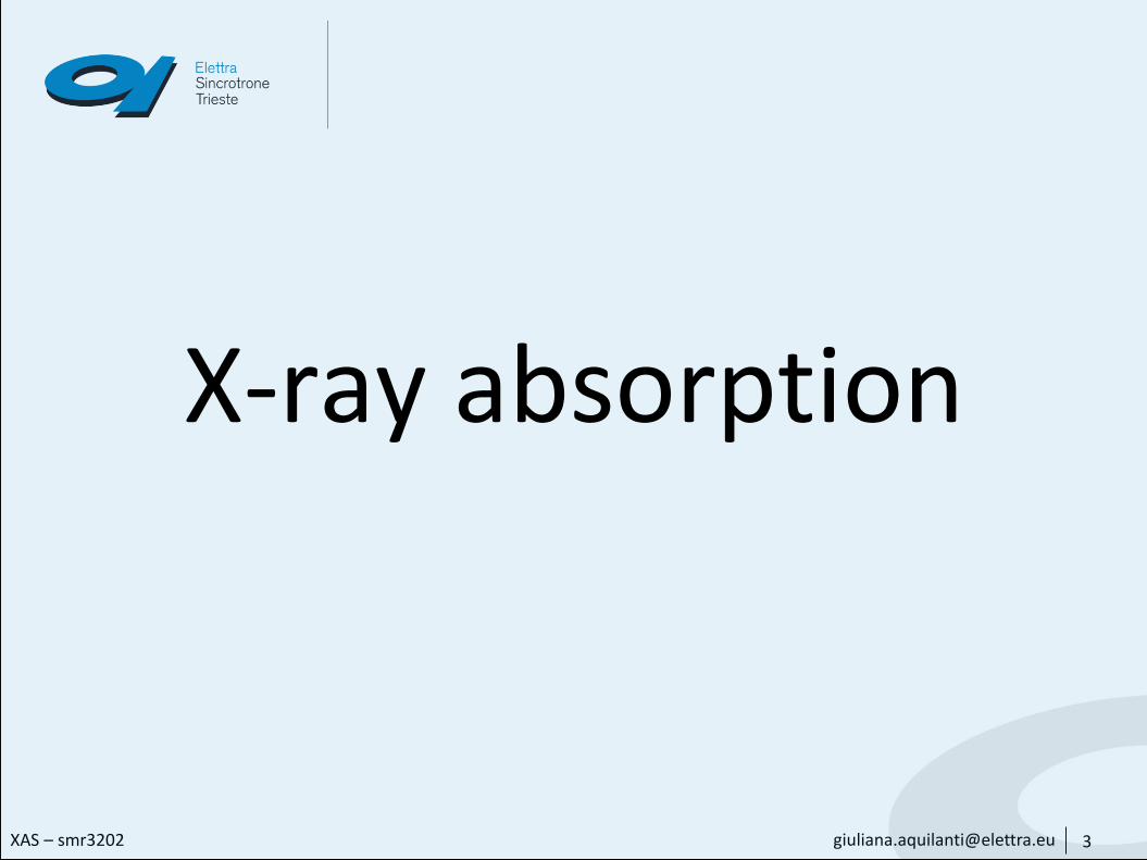
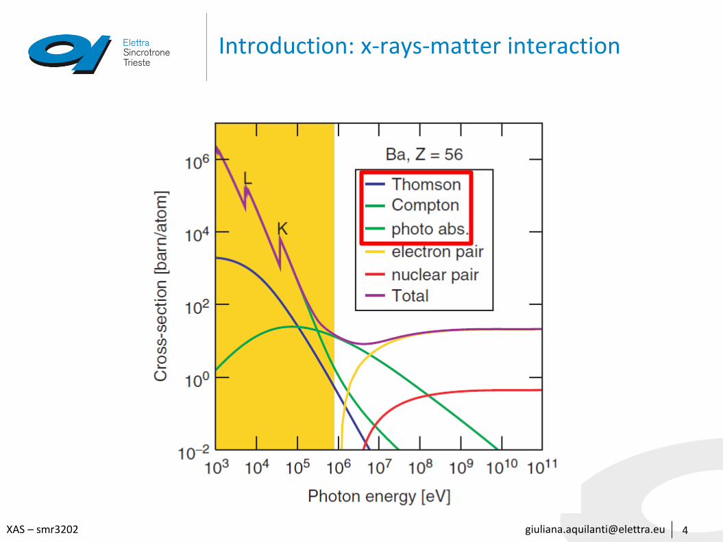
X-rays – matter interaction
• Photoelectric absorption
one photon is absorbed and the atom is ionized or excited
• Scattering
photons are deflected form the original trajectory by collision with an electron
• Elastic (Thomson scattering): the photon wavelength is unmodified by the scattering process
• Inelastic (Compton scattering): the photon wavelength is modified
5
[email protected] – smr3202
Main x-ray experimental techniques
• Spectroscopy
atomic and electronic structure of matter
• Absorption • Emission • Photoelectron spectroscopy
• Imaging
macroscopic pictures of a sample, based on the different absorption of x-rays by
different parts of the sample (medical radiography and x-ray microscopy)
• Scattering
• Elastic: Microscopic geometrical structure of condensed systems• Inelastic: Collective excitations
7
[email protected] – smr3202
Spectroscopic methods
8
• They measure the response of a system as a function of energy
• The energy that is scanned can be that of the incident beam or the energy of the outgoing particles (photons in x-ray fluorescence, electrons in photoelectron spectroscopy)
[email protected] – smr3202
The absorption coefficient - 1
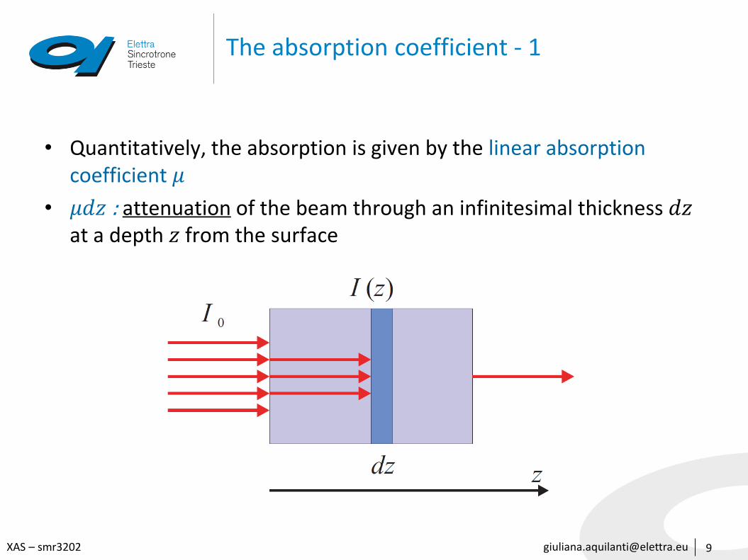
• Quantitatively, the absorption is given by the linear absorption coefficient 𝜇
• 𝜇𝑑𝑧 : attenuation of the beam through an infinitesimal thickness 𝑑𝑧at a depth 𝑧 from the surface
9
[email protected] – smr3202
The absorption coefficient - 2
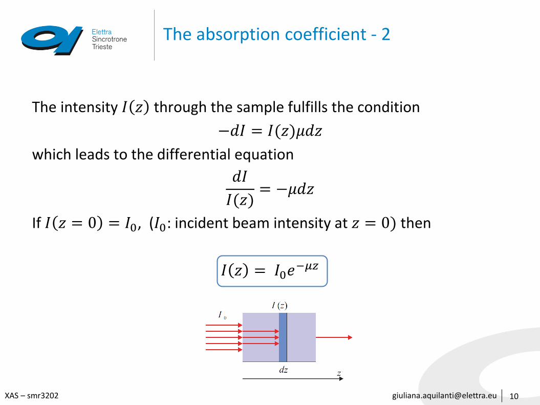
The intensity 𝐼 𝑧 through the sample fulfills the condition
−𝑑𝐼 = 𝐼(𝑧)𝜇𝑑𝑧
which leads to the differential equation
𝑑𝐼
𝐼(𝑧)= −𝜇𝑑𝑧
If 𝐼 𝑧 = 0 = 𝐼0, (𝐼0: incident beam intensity at 𝑧 = 0) then
𝐼 𝑧 = 𝐼0𝑒−𝜇𝑧
10
[email protected] – smr3202
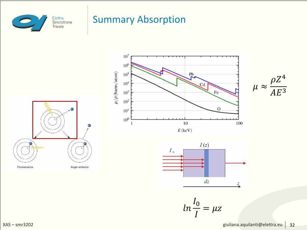
The absorption coefficient - 3
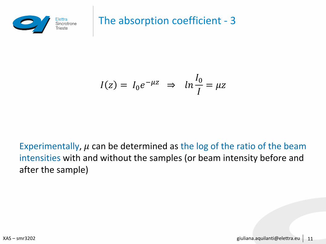
𝐼 𝑧 = 𝐼0𝑒−𝜇𝑧 ⇒ 𝑙𝑛
𝐼0𝐼
= 𝜇𝑧
Experimentally, 𝜇 can be determined as the log of the ratio of the beam intensities with and without the samples (or beam intensity before and after the sample)
11
[email protected] – smr3202
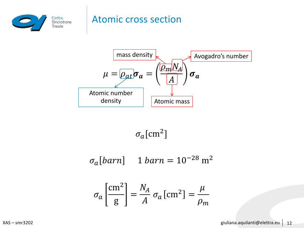
Atomic cross section
𝜇 = 𝜌𝑎𝑡𝝈𝒂 =𝜌𝑚𝑁𝐴
𝐴𝝈𝒂
𝜎𝑎[cm2]
𝜎𝑎 𝑏𝑎𝑟𝑛 1 𝑏𝑎𝑟𝑛 = 10−28 m2
𝜎𝑎
cm2
g=
𝑁𝐴
𝐴𝜎𝑎 cm2 =
𝜇
𝜌𝑚
12
Avogadro’s numbermass density
Atomic massAtomic number
density
[email protected] – smr3202
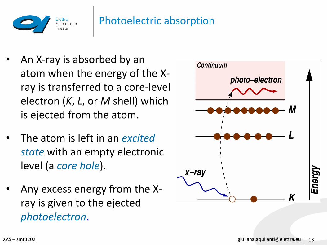
Photoelectric absorption
• An X-ray is absorbed by an atom when the energy of the X-ray is transferred to a core-level electron (K, L, or M shell) which is ejected from the atom.
• The atom is left in an excited state with an empty electronic level (a core hole).
• Any excess energy from the X-ray is given to the ejected photoelectron.
13
[email protected] – smr3202
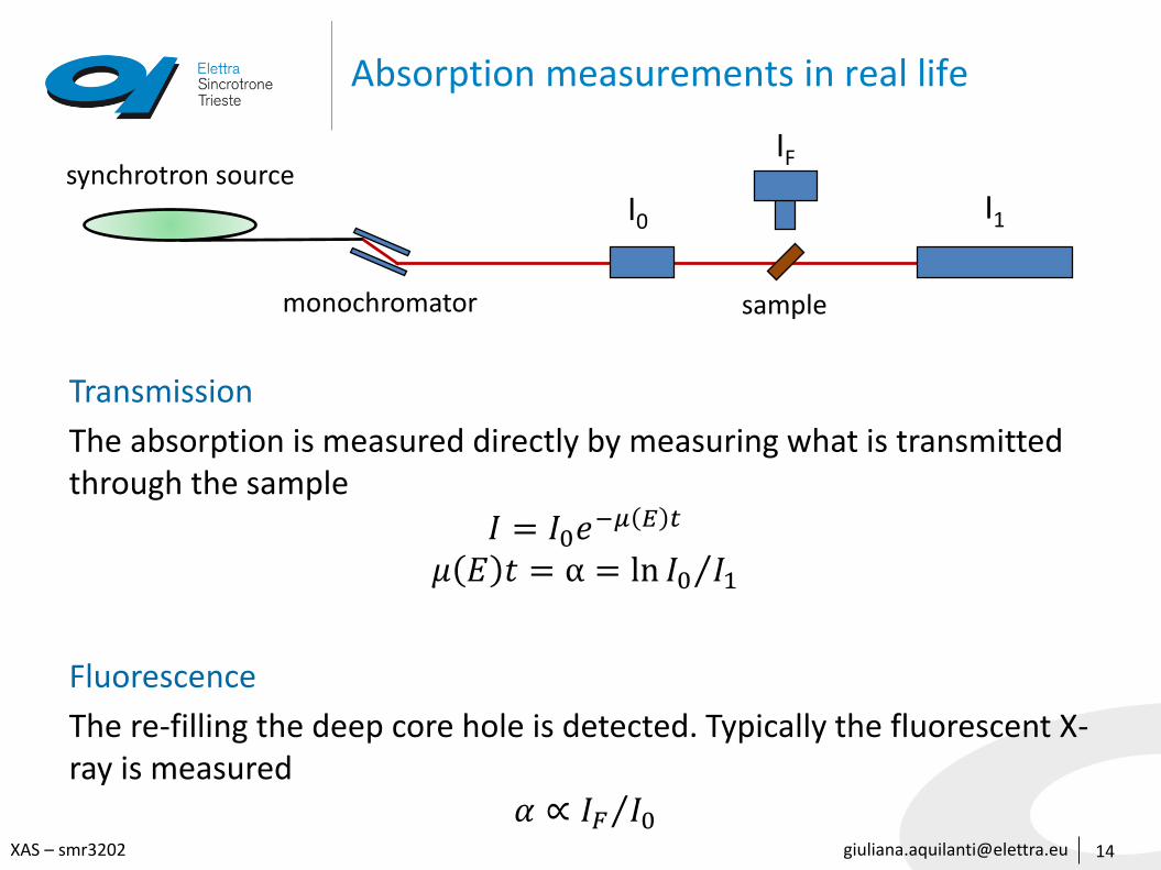
Absorption measurements in real life
14
Transmission
The absorption is measured directly by measuring what is transmitted through the sample
𝐼 = 𝐼0𝑒−𝜇 𝐸 𝑡
𝜇 𝐸 𝑡 = α = ln 𝐼0 𝐼1
Fluorescence
The re-filling the deep core hole is detected. Typically the fluorescent X-ray is measured
𝛼 ∝ 𝐼𝐹 𝐼0
synchrotron source
monochromator sample
I0
IF
I1
[email protected] – smr3202
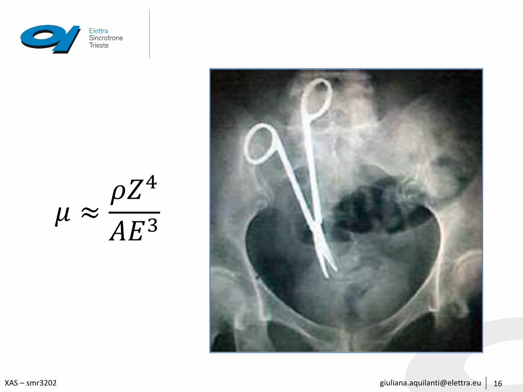
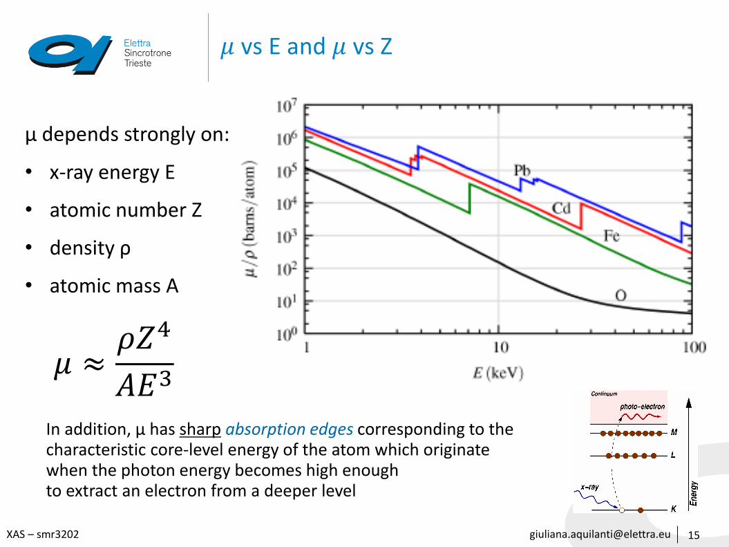
𝜇 vs E and 𝜇 vs Z
15
μ depends strongly on:
• x-ray energy E
• atomic number Z
• density ρ
• atomic mass A
In addition, μ has sharp absorption edges corresponding to the characteristic core-level energy of the atom which originatewhen the photon energy becomes high enough to extract an electron from a deeper level
𝜇 ≈𝜌𝑍4
𝐴𝐸3
[email protected] – smr3202
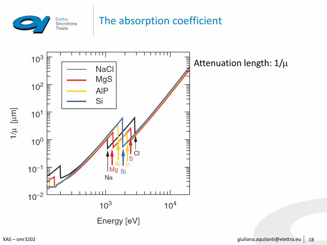
The absorption coefficient
• It is element-specific and a function of the x-ray energy
• It increases with the atomic number of the element (∝ 𝑍4)
• It decreases with increasing photon energy (∝ 𝐸−3)
• The absorption coefficient is essentially an indication of the electron density in the material and the electron binding energy.
• For instance, if a particular chemical substance can assume different geometric (‘allotropic’) forms and thereby have different densities, will be different accordingly
• Conversely, compounds that are chemically distinct but contain the same number of electrons per formula unit and have similar mass densities will have similar absorption properties (except close to absorption edges).
17
[email protected] – smr3202
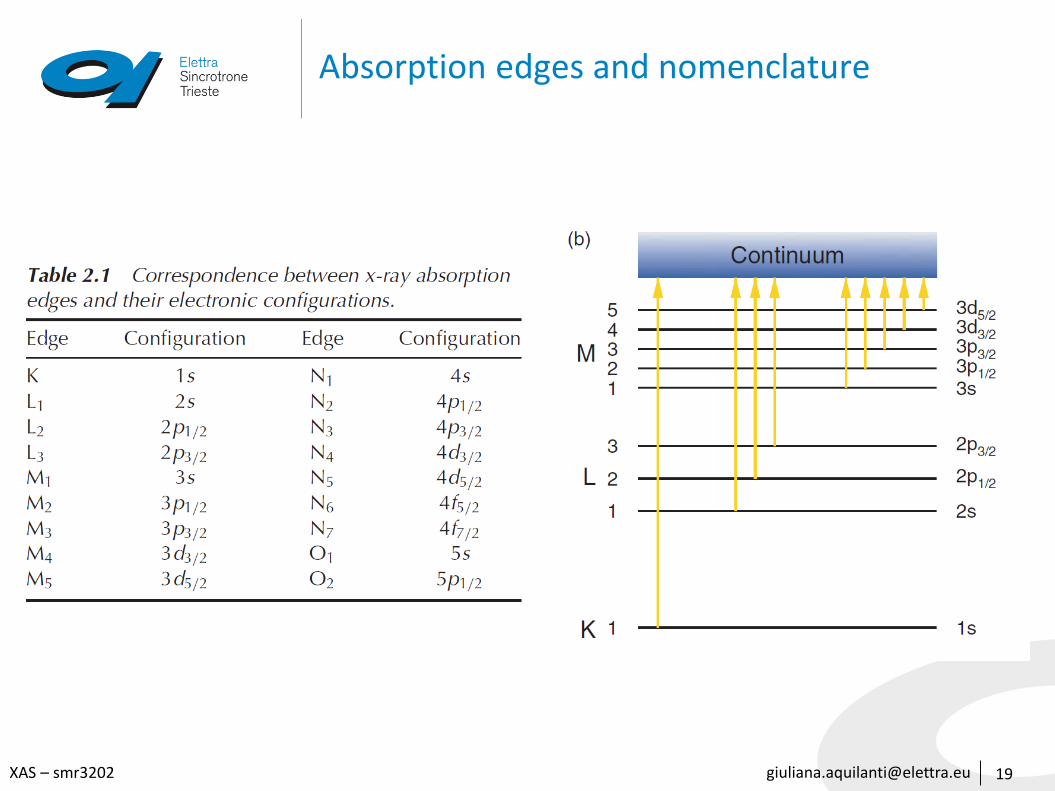
Absorption edge energies
20
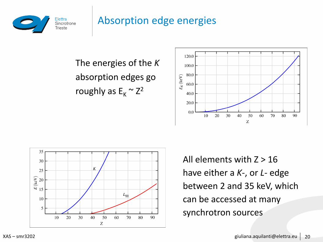
The energies of the K
absorption edges go
roughly as EK ~ Z2
All elements with Z > 16
have either a K-, or L- edge
between 2 and 35 keV, which
can be accessed at many
synchrotron sources
[email protected] – smr3202
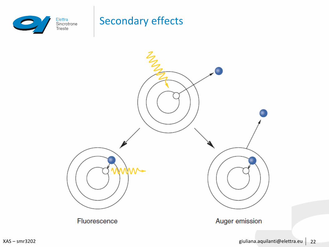
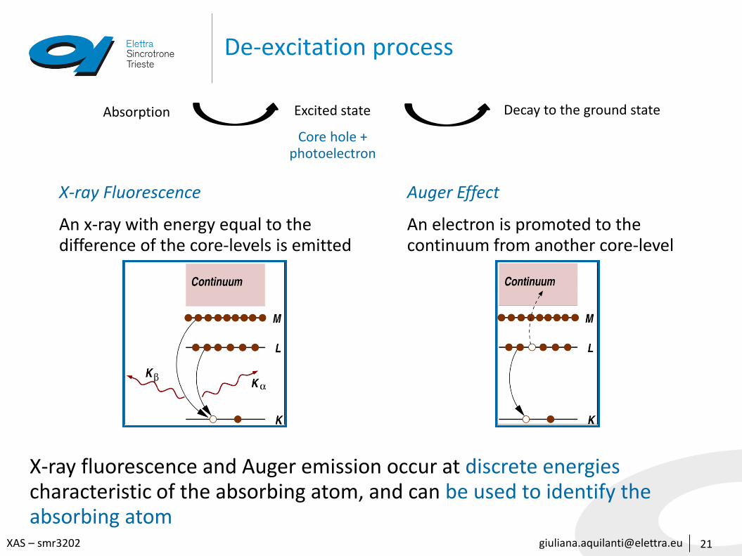
De-excitation process
21
Absorption Excited state
Core hole +photoelectron
Decay to the ground state
X-ray Fluorescence
An x-ray with energy equal to the difference of the core-levels is emitted
X-ray fluorescence and Auger emission occur at discrete energies characteristic of the absorbing atom, and can be used to identify the absorbing atom
Auger Effect
An electron is promoted to the continuum from another core-level
[email protected] – smr3202
X-ray fluorescence
• These characteristic x-ray lines result from the transition of an outer-shell electron relaxing to the hole left behind by the ejection of the photoelectron from the atom.
• This occurs on a timescale of the order of 10 to 100 fs.
• As the energy difference between the two involved levels is well defined, these lines are exceedingly sharp.
• From Heisenberg’s uncertainty principle Δ𝐸Δ𝑡 ∼ ℏ, the natural linewidth is therefore of the order of 0.01 eV, although this depends on the element and the transition
23
[email protected] – smr3202
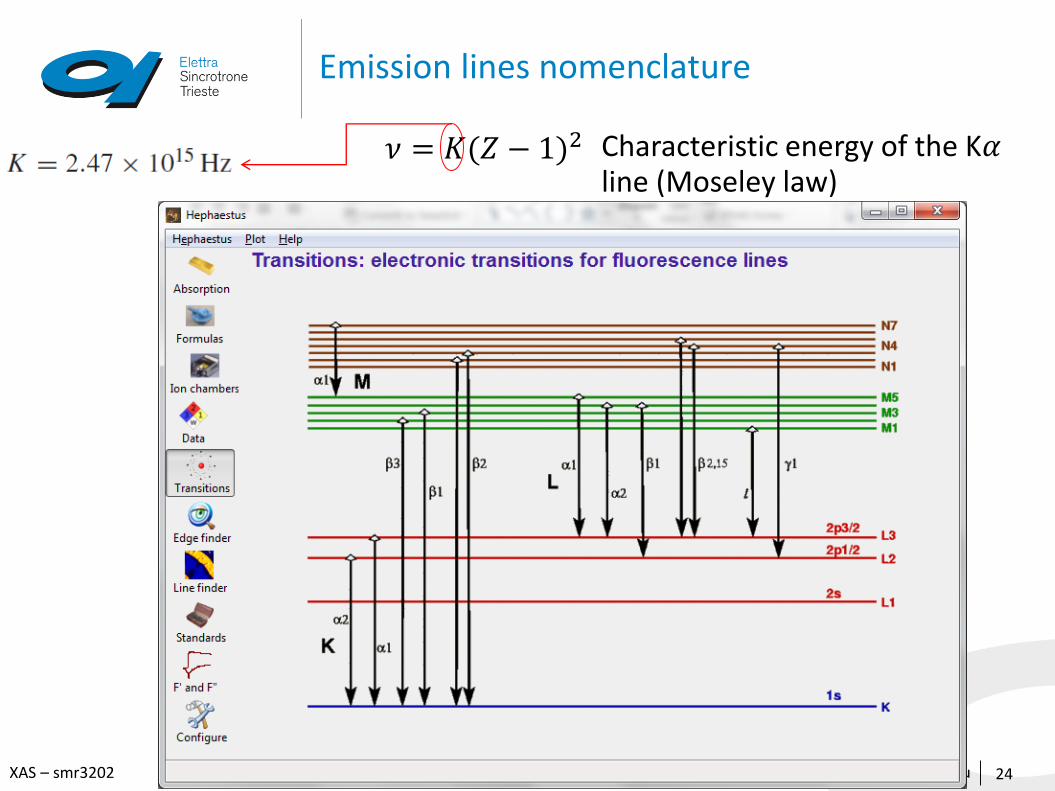
Emission lines nomenclature
24
𝜈 = 𝐾(𝑍 − 1)2 Characteristic energy of the K𝛼line (Moseley law)
[email protected] – smr3202
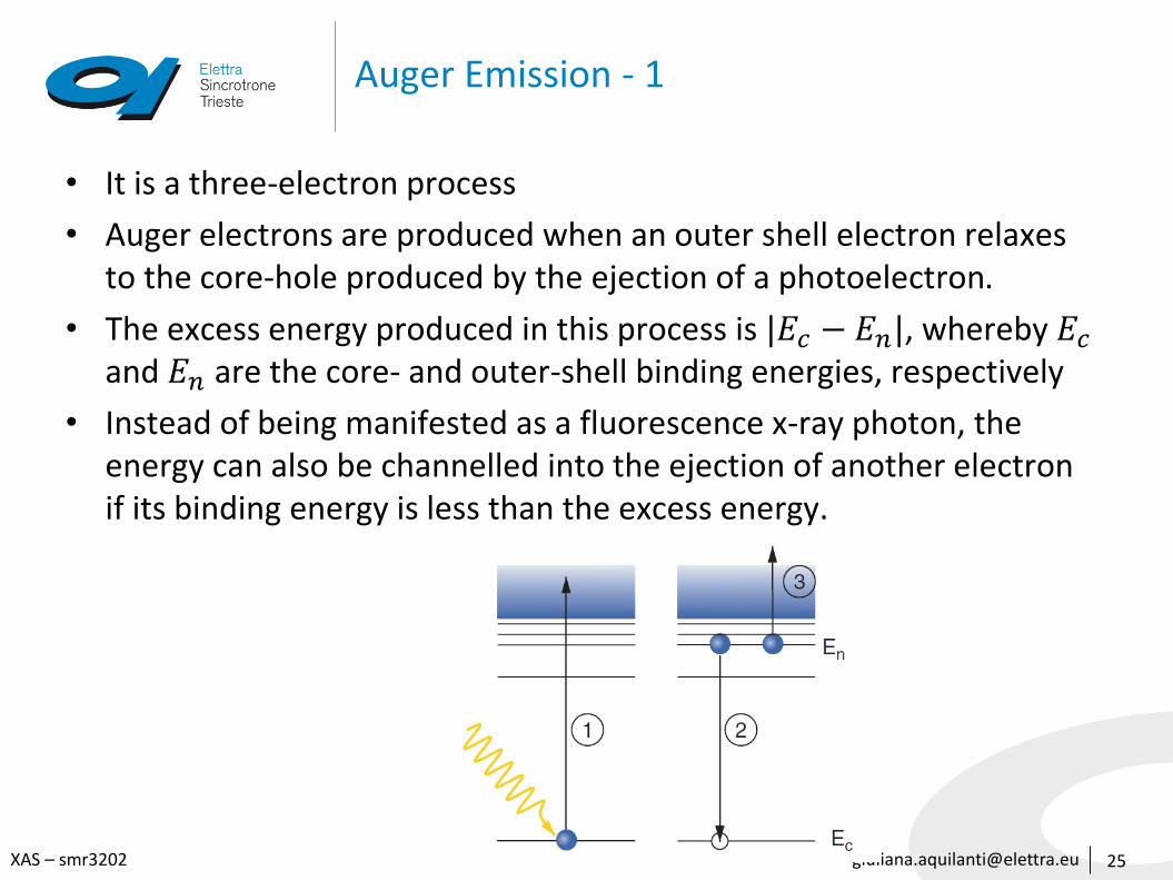
Auger Emission - 1
• It is a three-electron process
• Auger electrons are produced when an outer shell electron relaxes to the core-hole produced by the ejection of a photoelectron.
• The excess energy produced in this process is |𝐸𝑐 − 𝐸𝑛|, whereby 𝐸𝑐
and 𝐸𝑛 are the core- and outer-shell binding energies, respectively
• Instead of being manifested as a fluorescence x-ray photon, the energy can also be channelled into the ejection of another electron if its binding energy is less than the excess energy.
25
[email protected] – smr3202
Auger Emission - 2
• In case the Auger electron comes from the same shell as that of the electron which relaxed to the core-level hole, then the electron energy is |𝐸𝑐 − 2𝐸𝑛|
• More generally, the kinetic energy is |𝐸𝑐 − 𝐸𝑛 − 𝐸𝑚′|, where 𝐸𝑚′ is the binding energy of the Auger electron. The prime shows that the binding energy of this level has been changed (normally increased) because the electron ejected from this level originates from an already ionized atom.
• Typical Auger electron energies are in the range of 100 to 500 eV which have escape depths of only a few nanometres, hence Auger spectroscopy is very surface sensitive.
• In contrast to photoelectrons, the energies of Auger electrons (|𝐸𝑐 − 𝐸𝑛 −𝐸𝑚′|) are independent of the incident photon energy, although the amount of Auger electrons emitted is directly proportional to the absorption cross-section in the surface region.
26

[email protected] – smr3202
Auger Emission - 2
• In case the Auger electron comes from the same shell as that of the electron which relaxed to the core-level hole, then the electron energy is |𝐸𝑐 − 2𝐸𝑛|
• More generally, the kinetic energy is |𝐸𝑐 − 𝐸𝑛 − 𝐸𝑚′|, where 𝐸𝑚′ is the binding energy of the Auger electron. The prime shows that the binding energy of this level has been changed (normally increased) because the electron ejected from this level originates from an already ionized atom.
• Typical Auger electron energies are in the range of 100 to 500 eV which have escape depths of only a few nanometres, hence Auger spectroscopy is very surface sensitive.
• In contrast to photoelectrons, the energies of Auger electrons (|𝐸𝑐 − 𝐸𝑛 −𝐸𝑚′|) are independent of the incident photon energy, although the amount of Auger electrons emitted is directly proportional to the absorption cross-section in the surface region.
27
[email protected] – smr3202
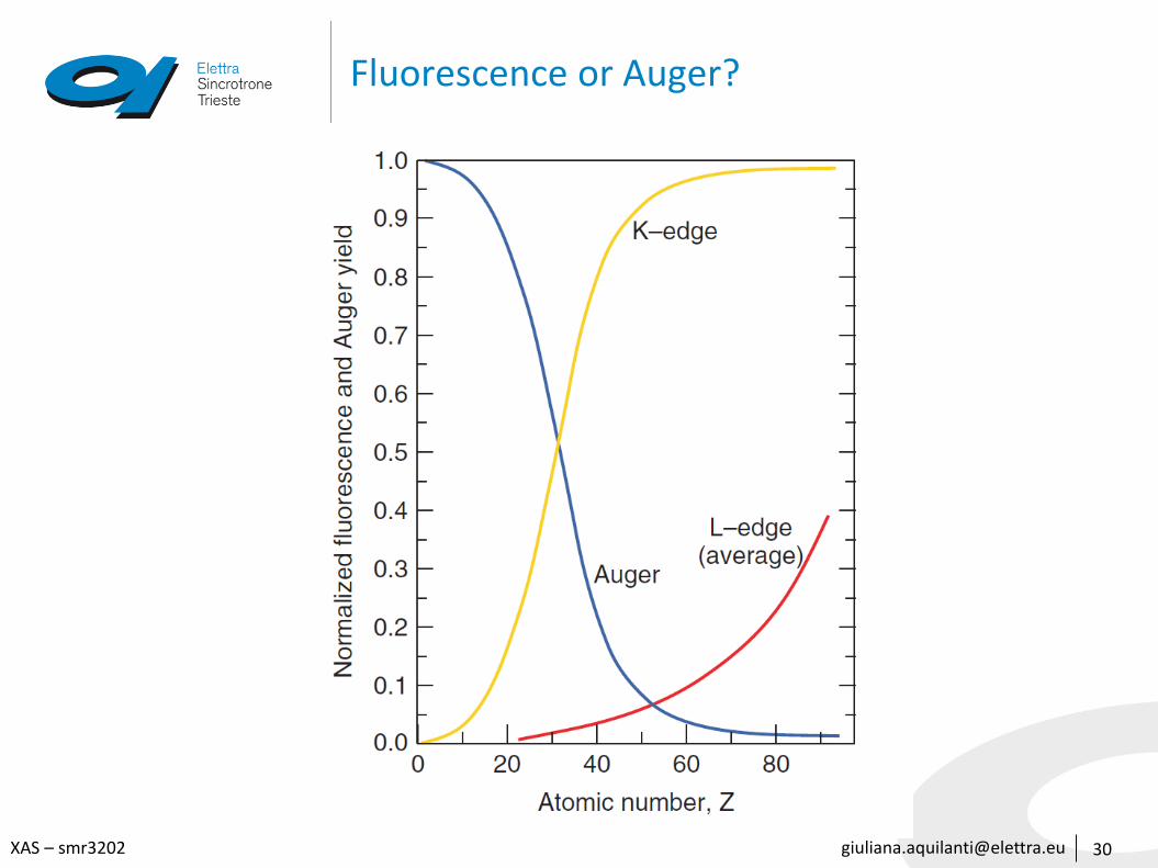
Fluorescence or Auger?
• Auger-electron emission and x-ray fluorescence are competitive processes
• The rate of spontaneous fluorescence, is proportional to the third power of the energy difference between the upper and lower state.Hence, for a given atom, K-emission lines are more probable than L-emission
• Fluorescence is stronger for heavier atoms, which have a more attractive positive nuclear charge and therefore a larger energy difference separating adjacent shells
28
[email protected] – smr3202
Fluorescence or Auger?
• The probability of an Auger electron being emitted increases with decreasing energy difference between the excited atom and the atom after Auger emission.
• LMM events are more likely than KLL events.
• Low atomic-number atoms have higher Auger yields than do heavier atoms.
• High atomic-number elements have a large positive charge at the nucleus, which binds electrons more tightly, reducing the probability of Auger emission
29
[email protected] – smr3202
X-ray Absorption Fine Structure
34
9.4 9.6 9.8 10.0 10.2 10.4 10.6
0.5
1.0
1.5
2.0
2.5
3.0
mt(
E) (
arb
. un
its.
)
Energy (keV)
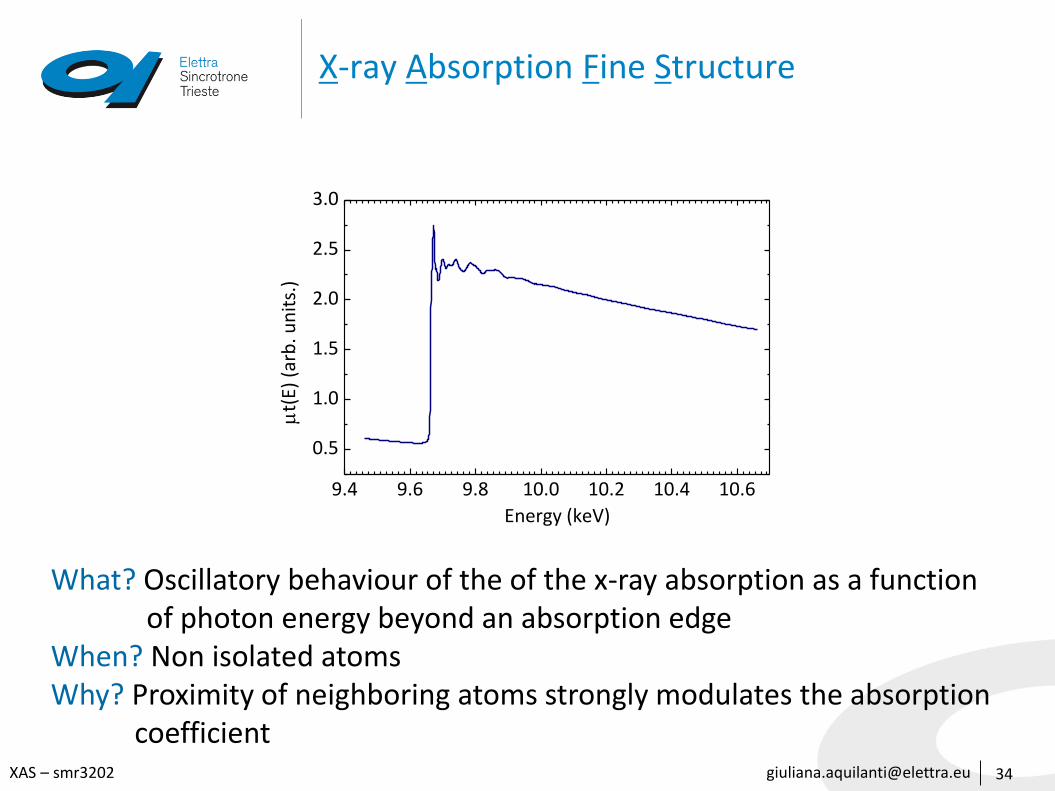
What? Oscillatory behaviour of the of the x-ray absorption as a function of photon energy beyond an absorption edge
When? Non isolated atomsWhy? Proximity of neighboring atoms strongly modulates the absorption
coefficient
[email protected] – smr3202
A little history
35
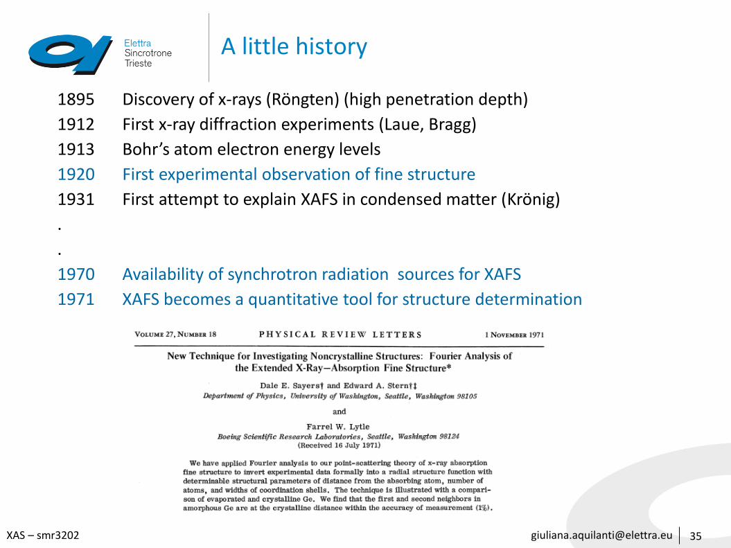
1895 Discovery of x-rays (Röngten) (high penetration depth)
1912 First x-ray diffraction experiments (Laue, Bragg)
1913 Bohr’s atom electron energy levels
1920 First experimental observation of fine structure
1931 First attempt to explain XAFS in condensed matter (Krönig)
.
.
1970 Availability of synchrotron radiation sources for XAFS
1971 XAFS becomes a quantitative tool for structure determination
[email protected] – smr3202
XANES and EXAFS - 1
36
9.4 9.6 9.8 10.0 10.2 10.4 10.6
0.5
1.0
1.5
2.0
2.5
3.0
mt(
E) (
arb
. un
its.
)
Energy (keV)
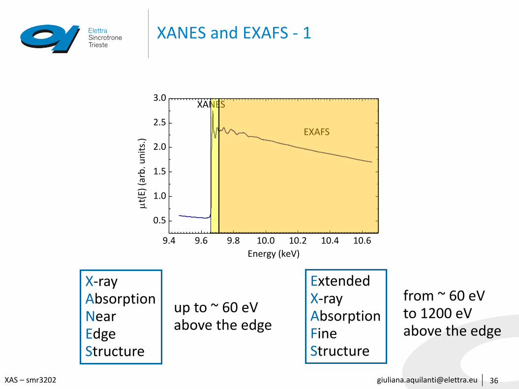
XANES
EXAFS
ExtendedX-rayAbsorptionFine Structure
X-rayAbsorptionNear EdgeStructure
up to ~ 60 eVabove the edge
from ~ 60 eV to 1200 eVabove the edge
[email protected] – smr3202
XANES and EXAFS - 2
37
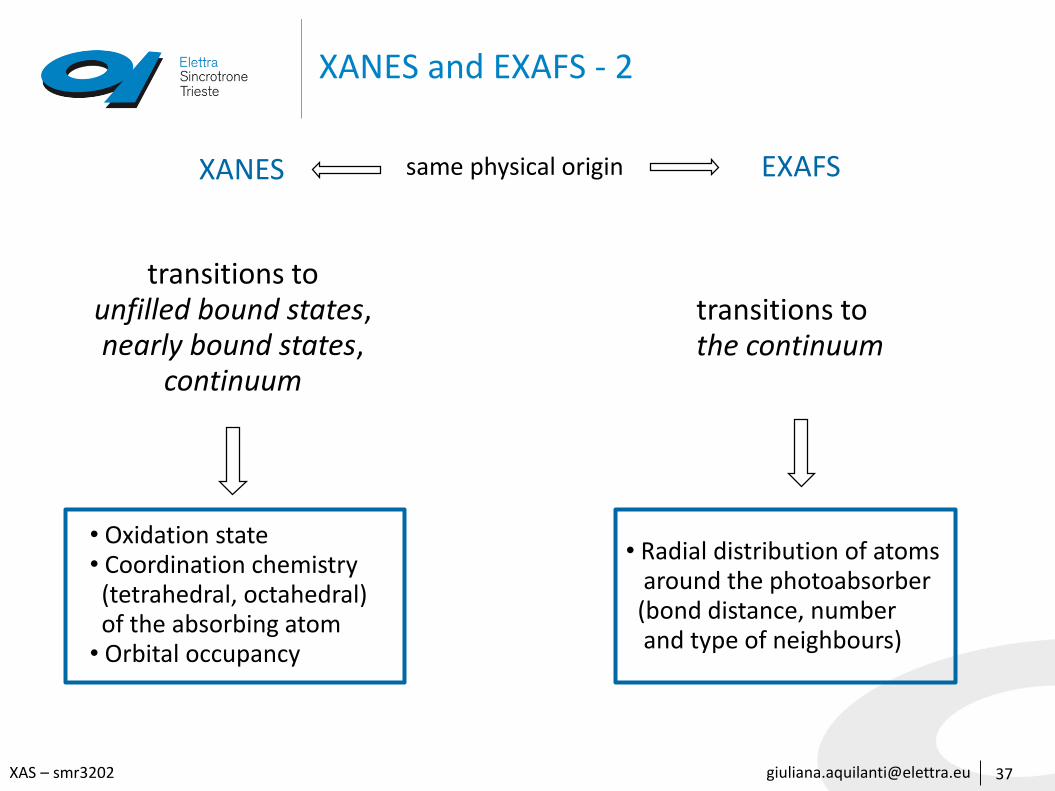
XANES EXAFSsame physical origin
transitions to unfilled bound states, nearly bound states,
continuum
transitions to the continuum
• Oxidation state• Coordination chemistry (tetrahedral, octahedral) of the absorbing atom
• Orbital occupancy
• Radial distribution of atoms around the photoabsorber(bond distance, numberand type of neighbours)
[email protected] – smr3202
EXAFS qualitatively – isolated atom
38
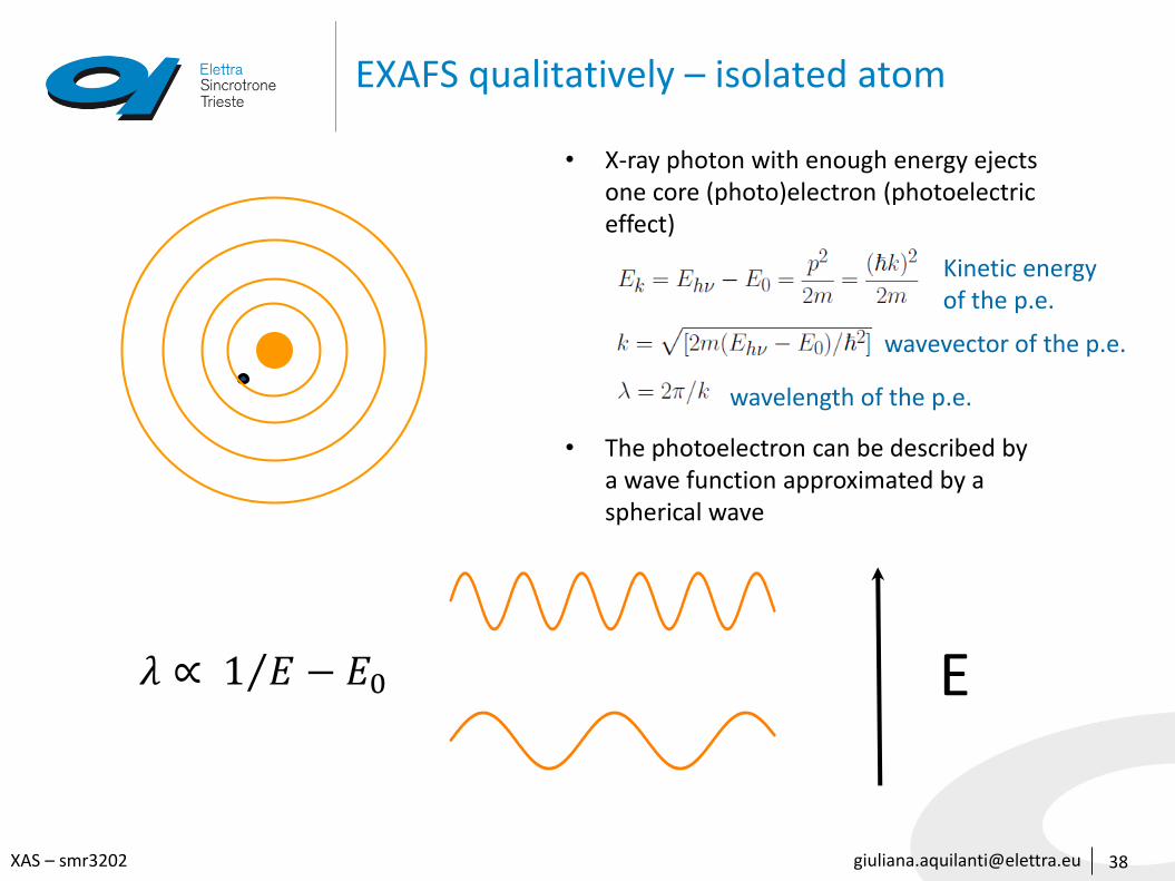
• X-ray photon with enough energy ejects one core (photo)electron (photoelectric effect)
• The photoelectron can be described by a wave function approximated by a spherical wave
Kinetic energyof the p.e.
wavevector of the p.e.
wavelength of the p.e.
E
38
𝜆 ∝ 1 𝐸 − 𝐸0
[email protected] – smr3202 39
EXAFS qualitatively – condensed matter
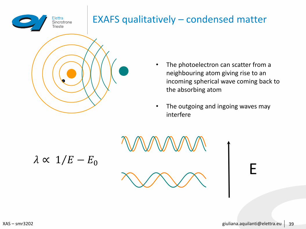
• The photoelectron can scatter from a neighbouring atom giving rise to an incoming spherical wave coming back to the absorbing atom
• The outgoing and ingoing waves may interfere
E𝜆 ∝ 1 𝐸 − 𝐸0
[email protected] – smr3202
Origin of the fine structure (oscillations)
• The interference between the outgoing and the scattering part of the photoelectron at the absorbing atom changes the probability for an absorption of x-rays i.e. alters the absorption coefficient μ(E) that is no longer smooth as in isolated atoms, but oscillates.
• In the extreme of destructive interference, when the outgoing and the backscattered waves are completely out of phase, they will cancel each other, which means that no free unoccupied state exists in which the core-electron could be excited to.
• Thus absorption is unlikely to occur and the EXAFS oscillations will have a minimum.
• The phase relationship between outgoing and incoming waves depends on photoelectron wavelength (and so on the energy of x-rays) and interatomic distance R.
• The amplitude is determined by the number and type of neighbours since they determine how strongly the photoelectron will be scattered
40
[email protected] – smr3202
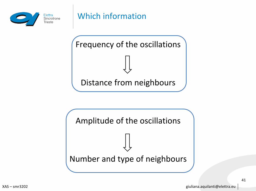
Which information
Frequency of the oscillations
Distance from neighbours
Amplitude of the oscillations
Number and type of neighbours
41
[email protected] – smr3202
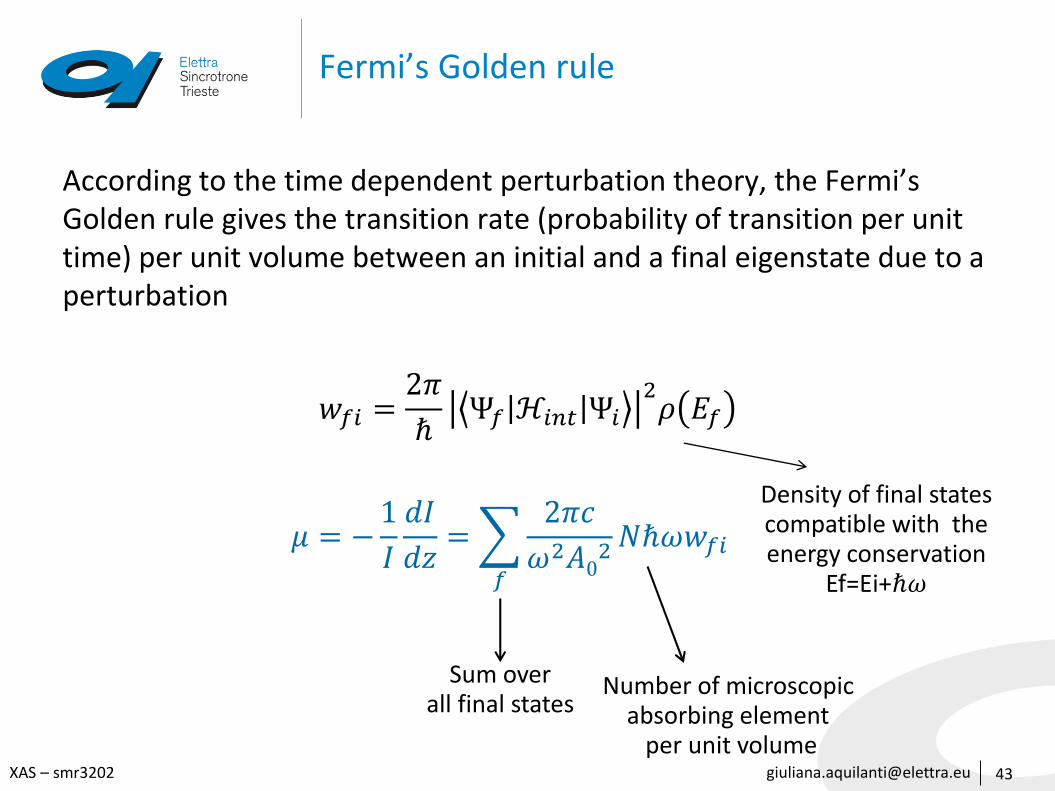
Fermi’s Golden rule
According to the time dependent perturbation theory, the Fermi’s Golden rule gives the transition rate (probability of transition per unit time) per unit volume between an initial and a final eigenstate due to a perturbation
𝑤𝑓𝑖 =2𝜋
ℏΨ𝑓 ℋ𝑖𝑛𝑡 Ψ𝑖
2𝜌 𝐸𝑓
𝜇 = −1
𝐼
𝑑𝐼
𝑑𝑧=
𝑓
2𝜋𝑐
𝜔2𝐴02𝑁ℏ𝜔𝑤𝑓𝑖
43
Sum overall final states
Number of microscopic absorbing element
per unit volume
Density of final statescompatible with the energy conservation
Ef=Ei+ℏ𝜔
[email protected] – smr3202
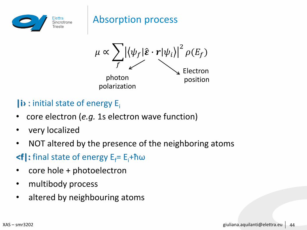
Absorption process
𝜇 ∝
𝑓
𝜓𝑓 𝜺 ∙ 𝒓 𝜓𝑖2𝜌(𝐸𝑓)
|i› : initial state of energy Ei
• core electron (e.g. 1s electron wave function)
• very localized
• NOT altered by the presence of the neighboring atoms
<f|: final state of energy Ef= Ei+ħω
• core hole + photoelectron
• multibody process
• altered by neighbouring atoms
44
photonpolarization
Electron position
[email protected] – smr3202
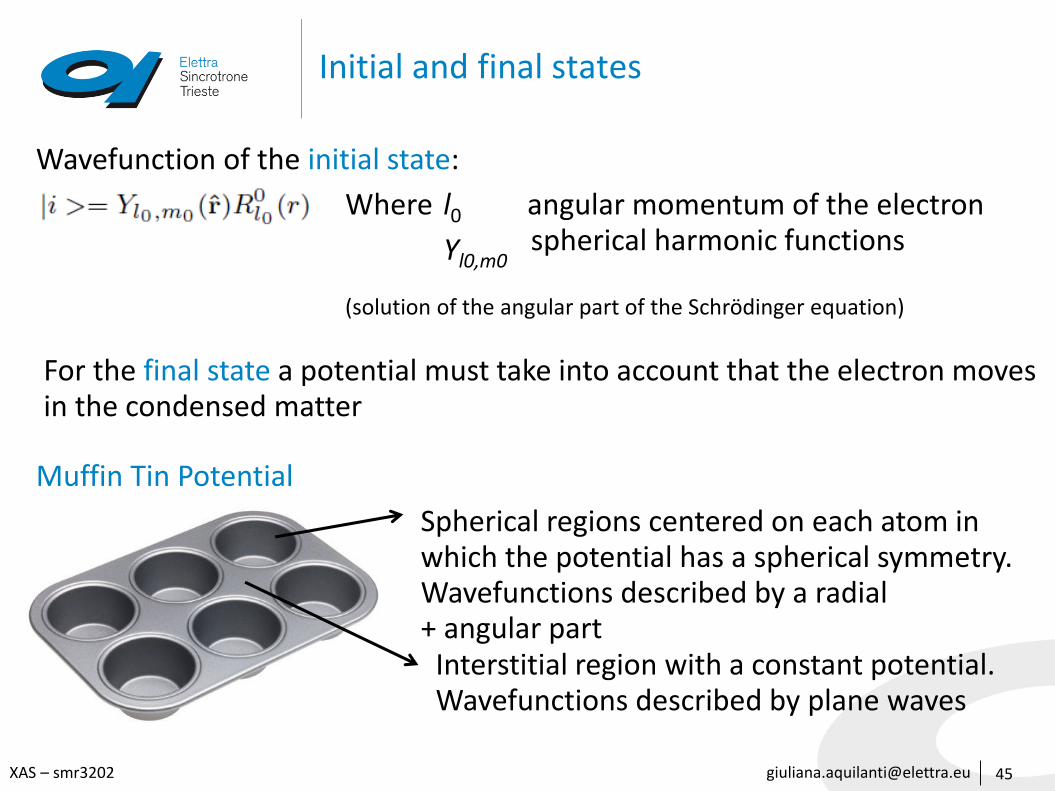
Initial and final states
45
Where: angular momentum of the electronspherical harmonic functions
(solution of the angular part of the Schrödinger equation)
l0
Wavefunction of the initial state:
Yl0,m0
l0
For the final state a potential must take into account that the electron movesin the condensed matter
Muffin Tin Potential
Spherical regions centered on each atom in which the potential has a spherical symmetry.Wavefunctions described by a radial + angular part
Interstitial region with a constant potential.Wavefunctions described by plane waves
[email protected] – smr3202
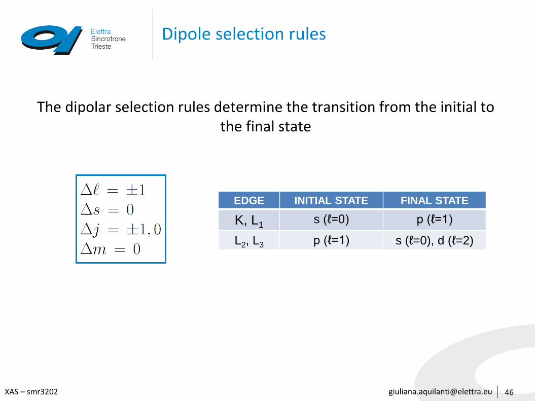
Dipole selection rules
The dipolar selection rules determine the transition from the initial to the final state
46
EDGE INITIAL STATE FINAL STATE
K, L1s (ℓ=0) p (ℓ=1)
L2, L3 p (ℓ=1) s (ℓ=0), d (ℓ=2)
[email protected] – smr3202
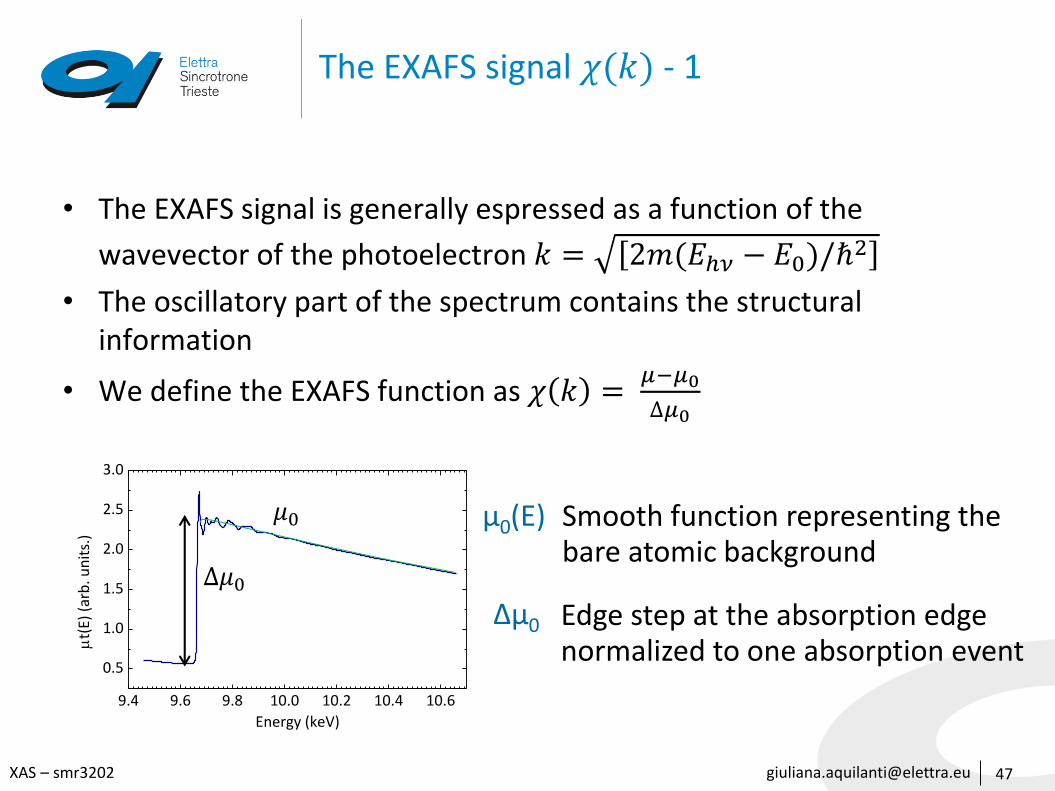
The EXAFS signal 𝜒(𝑘) - 1
• The EXAFS signal is generally espressed as a function of the
wavevector of the photoelectron 𝑘 = 2𝑚(𝐸ℎ𝜈 − 𝐸0)/ℏ2
• The oscillatory part of the spectrum contains the structural information
• We define the EXAFS function as 𝜒 𝑘 =𝜇−𝜇0
Δ𝜇0
47
9.4 9.6 9.8 10.0 10.2 10.4 10.6
0.5
1.0
1.5
2.0
2.5
3.0
mt(
E) (
arb
. un
its.
)
Energy (keV)
Δ𝜇0
𝜇0 μ0(E) Smooth function representing the bare atomic background
Δμ0 Edge step at the absorption edge normalized to one absorption event
[email protected] – smr3202
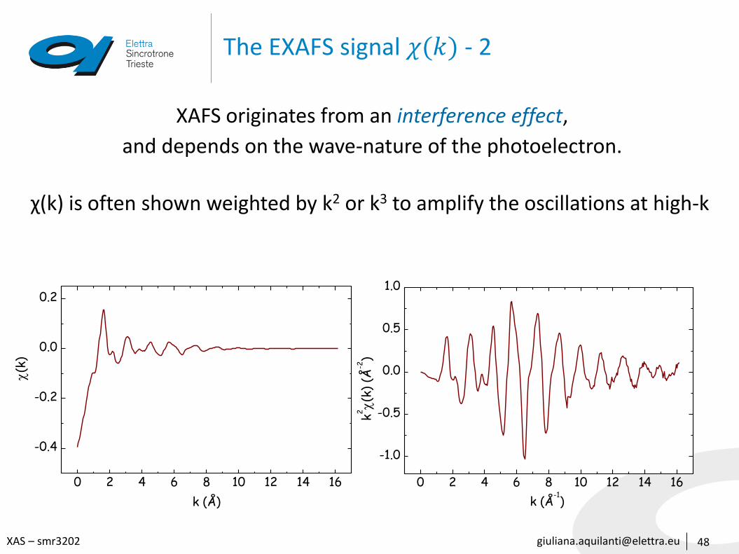
The EXAFS signal 𝜒(𝑘) - 2
48
XAFS originates from an interference effect,
and depends on the wave-nature of the photoelectron.
χ(k) is often shown weighted by k2 or k3 to amplify the oscillations at high-k
0 2 4 6 8 10 12 14 16
-0.4
-0.2
0.0
0.2
(k
)
k (Å)
0 2 4 6 8 10 12 14 16
-1.0
-0.5
0.0
0.5
1.0
k2
(k)
(Å-2
)
k (Å-1)
[email protected] – smr3202
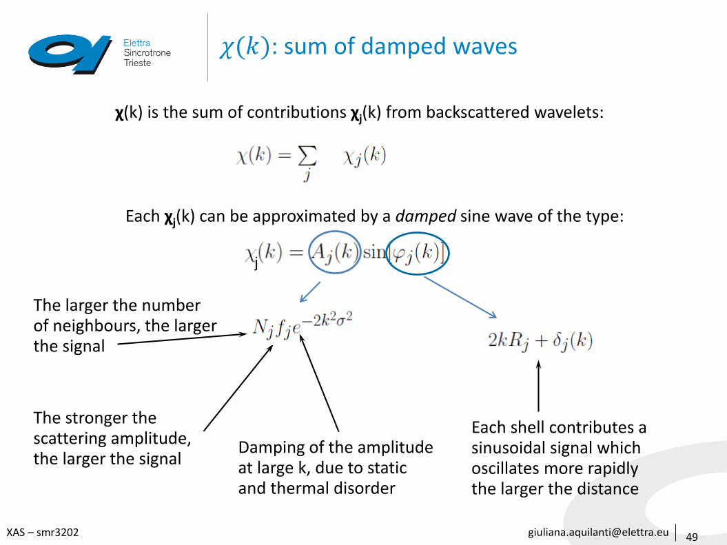
𝜒(𝑘): sum of damped waves
49
The larger the number of neighbours, the larger the signal
The stronger the scattering amplitude, the larger the signal
Each shell contributes a sinusoidal signal which oscillates more rapidly the larger the distance
χ(k) is the sum of contributions χj(k) from backscattered wavelets:
Each χj(k) can be approximated by a damped sine wave of the type:
Damping of the amplitude at large k, due to static and thermal disorder
j
[email protected] – smr3202
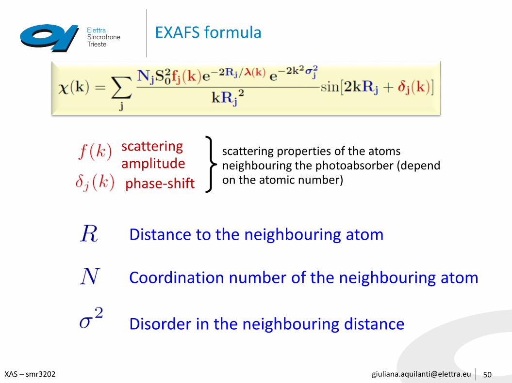
EXAFS formula
50
scattering properties of the atoms neighbouring the photoabsorber (dependon the atomic number)
scatteringamplitude
phase-shift
Distance to the neighbouring atom
Coordination number of the neighbouring atom
Disorder in the neighbouring distance
[email protected] – smr3202
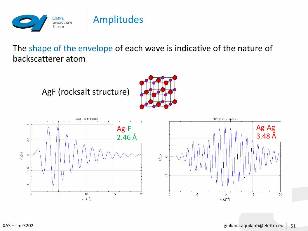
Amplitudes
51
AgF (rocksalt structure)
The shape of the envelope of each wave is indicative of the nature of backscatterer atom
Ag-F2.46 Å
Ag-Ag3.48 Å
[email protected] – smr3202
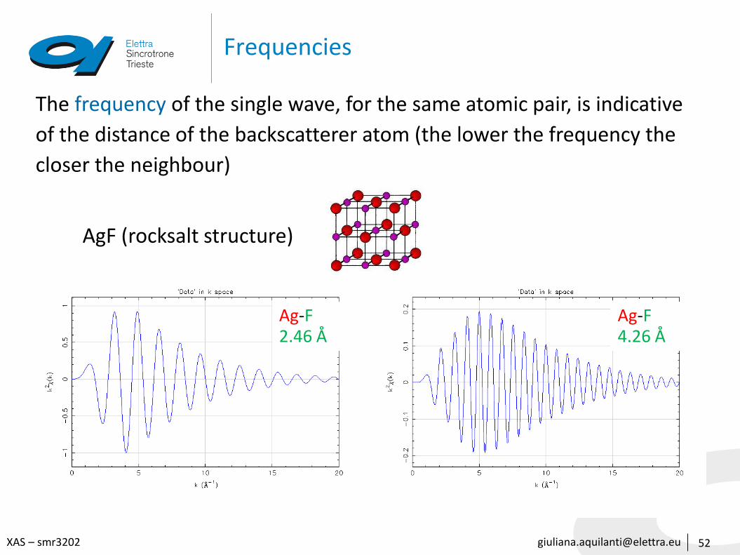
Frequencies
52
The frequency of the single wave, for the same atomic pair, is indicative
of the distance of the backscatterer atom (the lower the frequency the
closer the neighbour)
Ag-F2.46 Å
AgF (rocksalt structure)
Ag-F4.26 Å
[email protected] – smr3202
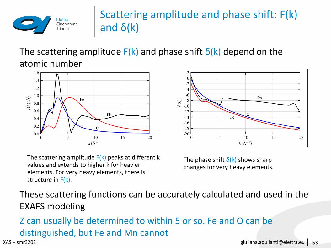
Scattering amplitude and phase shift: F(k) and δ(k)
The scattering amplitude F(k) and phase shift δ(k) depend on the atomic number
These scattering functions can be accurately calculated and used in the EXAFS modeling
Z can usually be determined to within 5 or so. Fe and O can be distinguished, but Fe and Mn cannot
53
The scattering amplitude F(k) peaks at different k values and extends to higher k for heavier elements. For very heavy elements, there is structure in F(k).
The phase shift δ(k) shows sharpchanges for very heavy elements.
[email protected] – smr3202
Multiple scattering
54
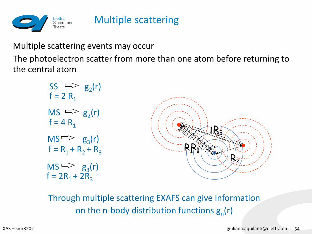
Multiple scattering events may occur
The photoelectron scatter from more than one atom before returning to the central atom
R1
SS g2(r)f = 2 R1
R1
MS g2(r)f = 4 R1
MS g3(r)f = R1 + R2 + R3
R1
R3
R2MS g3(r)f = 2R1 + 2R3
R1
R3
Through multiple scattering EXAFS can give information
on the n-body distribution functions gn(r)
[email protected] – smr3202
Qualitative picture of local coordination in R space
55
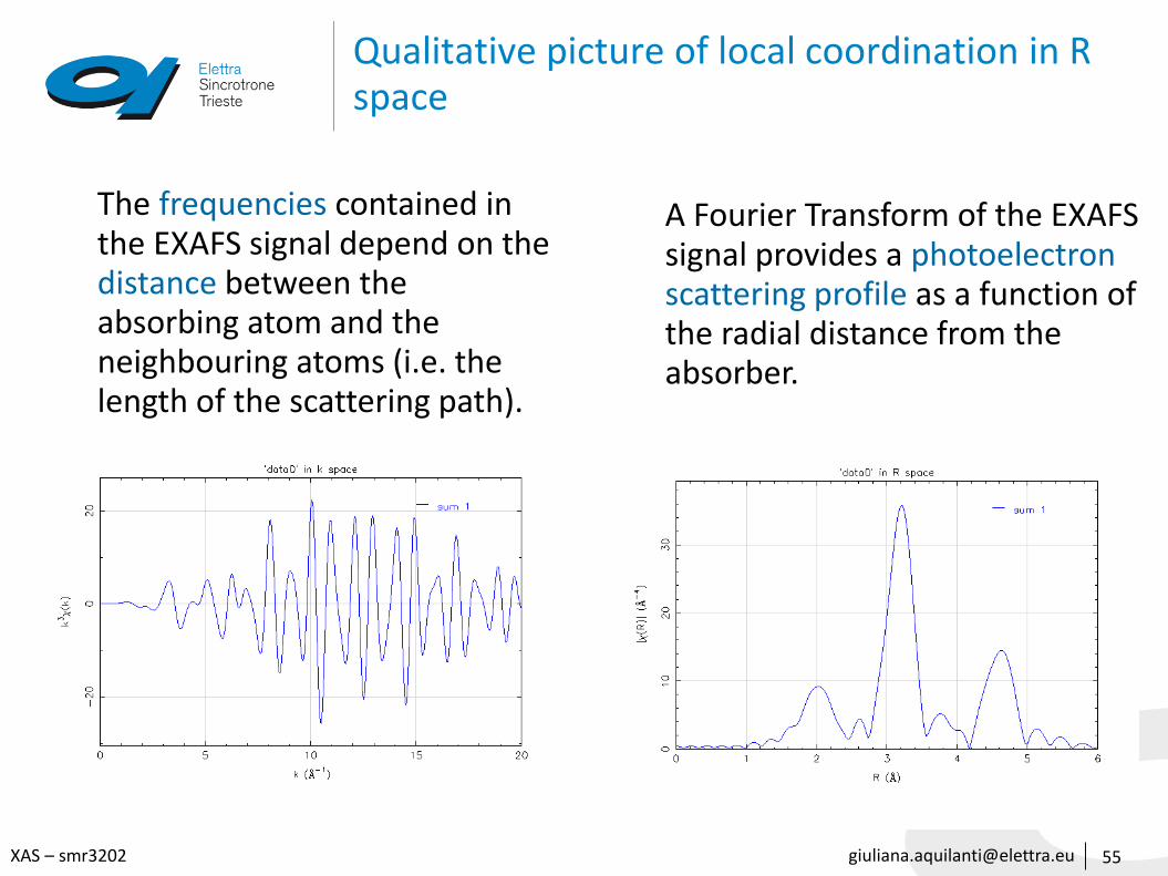
A Fourier Transform of the EXAFS signal provides a photoelectron scattering profile as a function of the radial distance from the absorber.
The frequencies contained in the EXAFS signal depend on the distance between the absorbing atom and the neighbouring atoms (i.e. the length of the scattering path).
[email protected] – smr3202
Quantitative structural determination
56
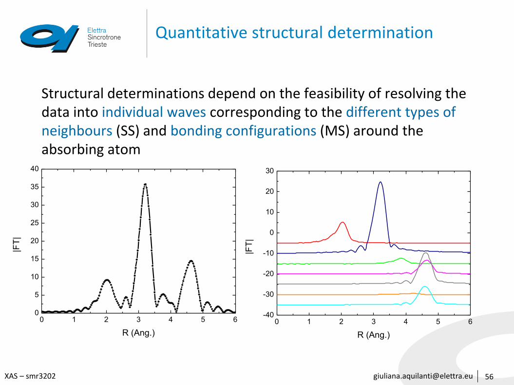
Structural determinations depend on the feasibility of resolving the data into individual waves corresponding to the different types of neighbours (SS) and bonding configurations (MS) around the absorbing atom
0 1 2 3 4 5 60
5
10
15
20
25
30
35
40
|FT
|
R (Ang.)
0 1 2 3 4 5 6-40
-30
-20
-10
0
10
20
30
|FT
|
R (Ang.)
[email protected] – smr3202
XAS vs diffraction methods
57
Diffraction Methods (x-rays, Neutrons)
• Crystalline materials with long-range ordering -> 3D picture of atomic coordinates
• Materials with only short-range order (amorphous solid, liquid, or solution) -> 1D RDF containing interatomic distances due to all atomic pairs in the sample
XAFS
• 1D radial distribution function (centered at the absorber)
• Higher sensitivity to local distortions (i.e. within the unit cell)• Charge state sensitivity (XANES)
• Element selectivity
• Structural information on the environment of each type of atom:
• distance, number, kind, static and thermal disorder
• 3-body correlations
[email protected] – smr3202
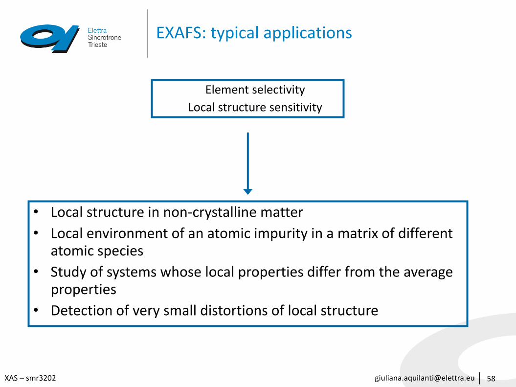
EXAFS: typical applications
58
• Local structure in non-crystalline matter
• Local environment of an atomic impurity in a matrix of different atomic species
• Study of systems whose local properties differ from the average properties
• Detection of very small distortions of local structure
Element selectivity
Local structure sensitivity
[email protected] – smr3202
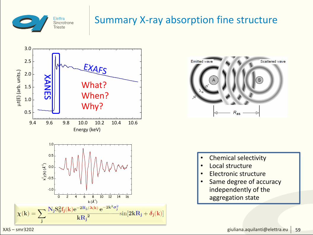
Summary X-ray absorption fine structure
59
9.4 9.6 9.8 10.0 10.2 10.4 10.6
0.5
1.0
1.5
2.0
2.5
3.0
mt(
E) (
arb
. un
its.
)
Energy (keV)
What?When?Why?
XA
NES
0 2 4 6 8 10 12 14 16
-1.0
-0.5
0.0
0.5
1.0
k2
(k)
(Å-2
)
k (Å-1)
XA
NES
• Chemical selectivity• Local structure• Electronic structure• Same degree of accuracy
independently of the aggregation state
[email protected] – smr3202
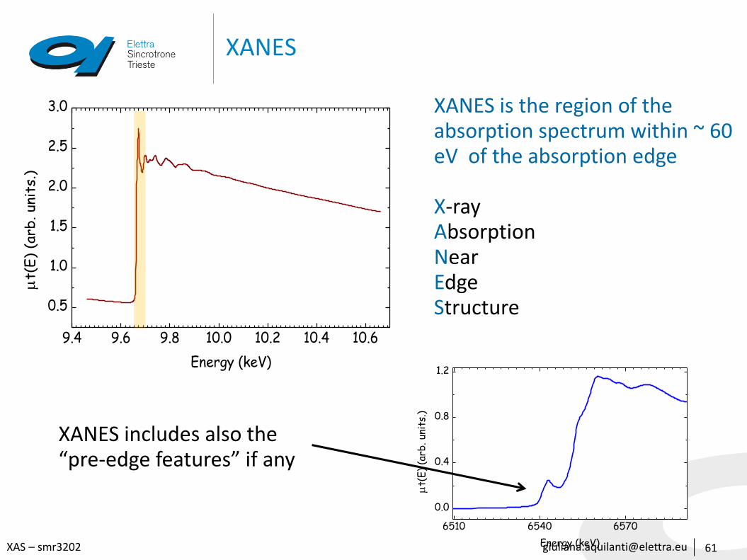
XANES
61
9.4 9.6 9.8 10.0 10.2 10.4 10.6
0.5
1.0
1.5
2.0
2.5
3.0
mt(
E)
(arb
. unit
s.)
Energy (keV)
XANES is the region of the absorption spectrum within ~ 60 eV of the absorption edge
X-ray Absorption Near Edge Structure
6510 6540 6570
0.0
0.4
0.8
1.2
mt(
E)
(arb
. un
its.
)
Energy (keV)
XANES includes also the “pre-edge features” if any
[email protected] – smr3202
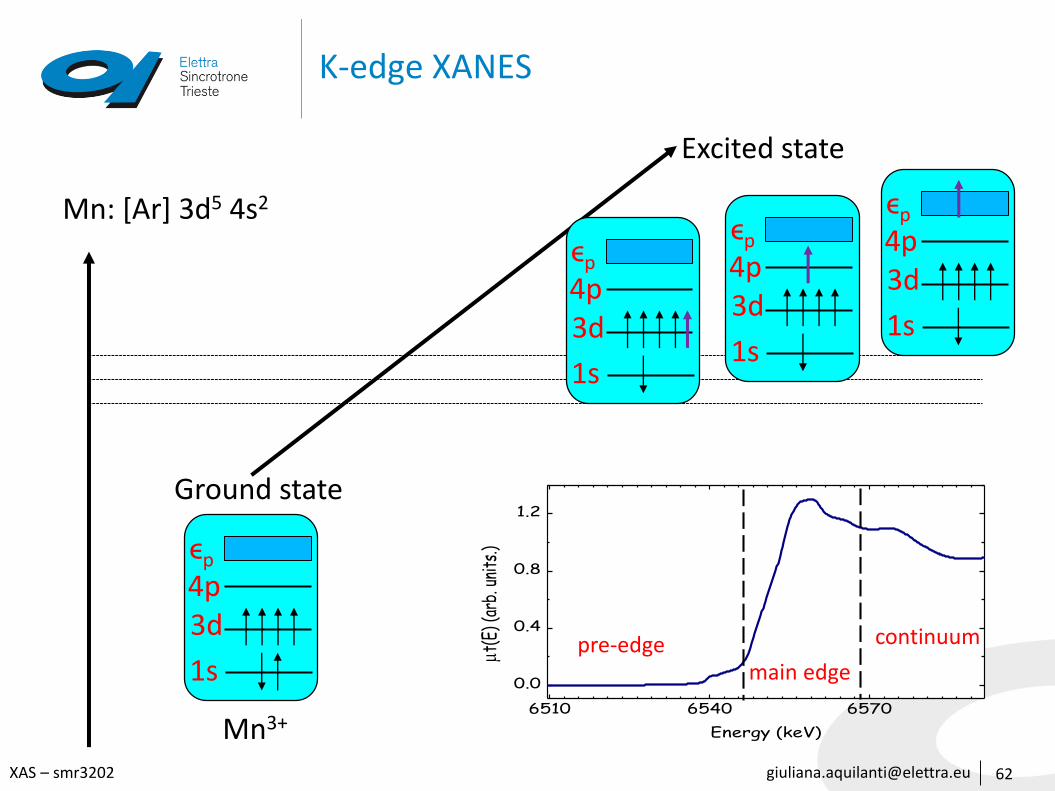
K-edge XANES
Mn: [Ar] 3d5 4s2
62
6510 6540 6570
0.0
0.4
0.8
1.2
mt(E
) (ar
b. u
nits
.)
Energy (keV)
pre-edgemain edge
continuum
1s
3d4pϵp
1s
3d4pϵp
1s
3d4pϵp
1s
3d4pϵp
Ground state
Excited state
Mn3+
[email protected] – smr3202
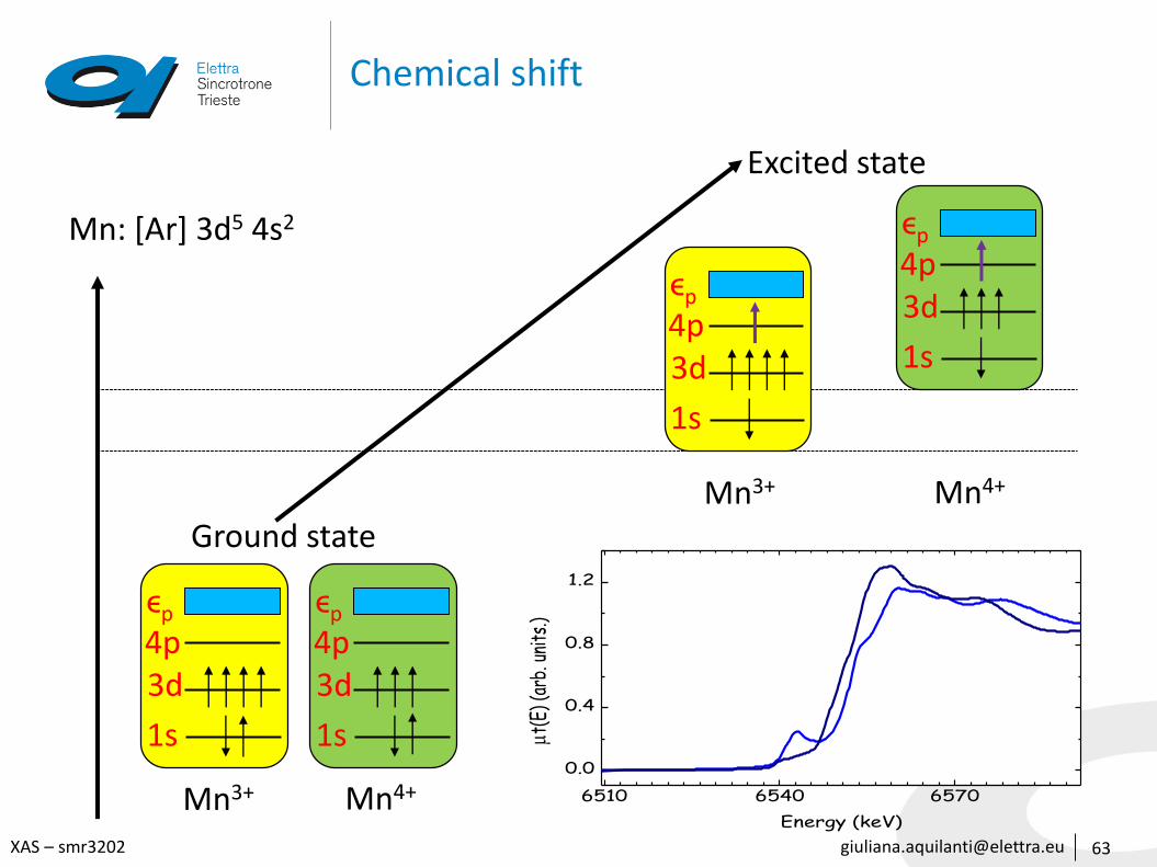
Chemical shift
63
Mn: [Ar] 3d5 4s2
1s
3d4pϵp
1s
3d4pϵp
1s
3d4pϵp
Ground state
Excited state
Mn3+ 6510 6540 6570
0.0
0.4
0.8
1.2
mt
(E) (
arb.
uni
ts.)
Energy (keV)
1s
3d4pϵp
Mn4+
Mn3+ Mn4+
[email protected] – smr3202
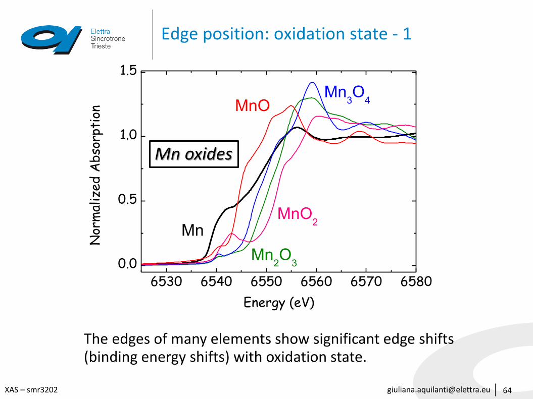
Edge position: oxidation state - 1
64
6530 6540 6550 6560 6570 6580
0.0
0.5
1.0
1.5
MnMnO
2
Mn2O
3
Mn3O
4
Nor
mal
ized A
bso
rpti
on
Energy (eV)
MnO
The edges of many elements show significant edge shifts(binding energy shifts) with oxidation state.
Mn oxides
[email protected] – smr3202
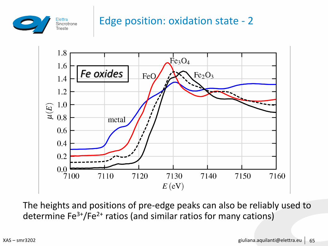
Edge position: oxidation state - 2
65
The heights and positions of pre-edge peaks can also be reliably used todetermine Fe3+/Fe2+ ratios (and similar ratios for many cations)
Fe oxides
[email protected] – smr3202
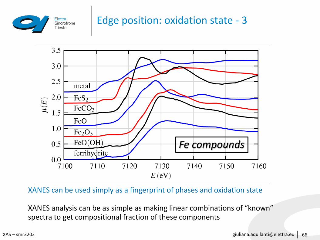
Edge position: oxidation state - 3
66
Fe compounds
XANES can be used simply as a fingerprint of phases and oxidation state
XANES analysis can be as simple as making linear combinations of “known” spectra to get compositional fraction of these components
[email protected] – smr3202
XANES transition
67
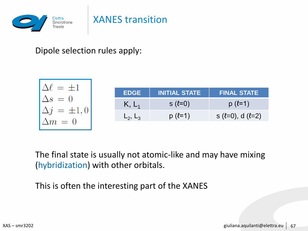
Dipole selection rules apply:
The final state is usually not atomic-like and may have mixing (hybridization) with other orbitals.
This is often the interesting part of the XANES
EDGE INITIAL STATE FINAL STATE
K, L1s (ℓ=0) p (ℓ=1)
L2, L3 p (ℓ=1) s (ℓ=0), d (ℓ=2)
[email protected] – smr3202
Transition metals pre-edge peaks
68
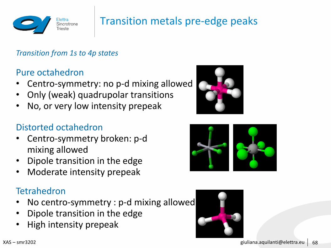
Transition from 1s to 4p states
Pure octahedron• Centro-symmetry: no p-d mixing allowed• Only (weak) quadrupolar transitions• No, or very low intensity prepeak
Distorted octahedron• Centro-symmetry broken: p-d
mixing allowed• Dipole transition in the edge• Moderate intensity prepeak
Tetrahedron• No centro-symmetry : p-d mixing allowed• Dipole transition in the edge• High intensity prepeak
[email protected] – smr3202
Prepeak: local coordination environment
69
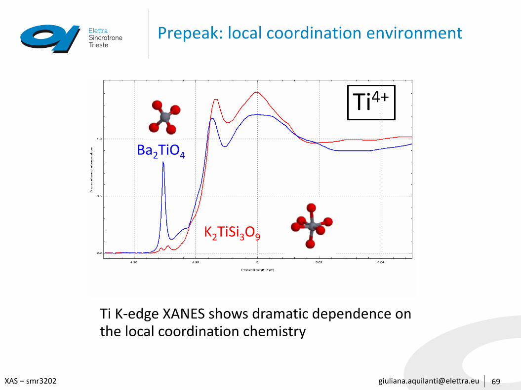
Ba2TiO4
K2TiSi3O9
Ti4+
Ti K-edge XANES shows dramatic dependence onthe local coordination chemistry
[email protected] – smr3202
Pre-peak : oxidation state
70
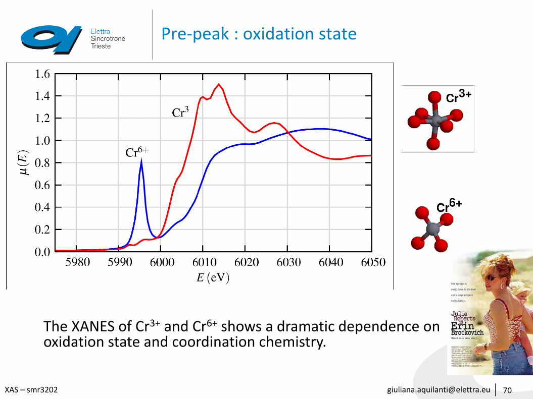
The XANES of Cr3+ and Cr6+ shows a dramatic dependence on oxidation state and coordination chemistry.
[email protected] – smr3202
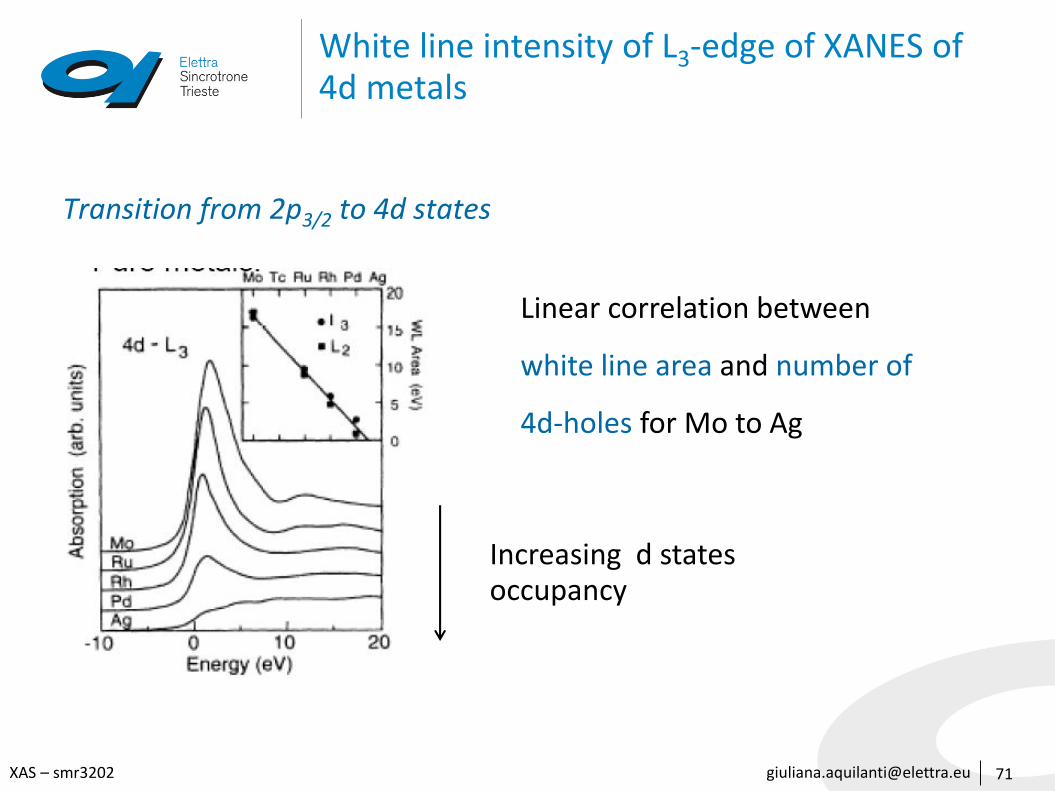
White line intensity of L3-edge of XANES of 4d metals
Transition from 2p3/2 to 4d states
71
Linear correlation between
white line area and number of
4d-holes for Mo to Ag
Increasing d statesoccupancy
[email protected] – smr3202
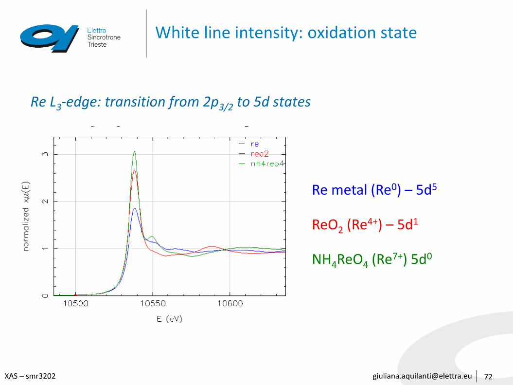
White line intensity: oxidation state
Re L3-edge: transition from 2p3/2 to 5d states
72
Re metal (Re0) – 5d5
ReO2 (Re4+) – 5d1
NH4ReO4 (Re7+) 5d0
[email protected] – smr3202
XANES: interpretation
The EXAFS equation breaks down at low-k, and the mean-free-path goes up.
This complicates XANES interpretation:
A simple equation for XANES does not exist
XANES can be described qualitatively (and nearly quantitatively) in terms of:
• Coordination chemistry: regular, distorted octahedral, tetrahedral, . . .
• Molecular orbitals: p-d orbital hybridization, crystal-field theory, . . .
• Band-structure: the density of available electronic states
• Multiple-scattering: multiple bounces of the photoelectron
73
[email protected] – smr3202
XANES: conclusions
XANES is a much larger signal than EXAFS
• XANES can be done at lower concentrations, and less-than-perfect sample conditions
XANES is easier to crudely interpret than EXAFS
• For many systems, the XANES analysis based on linear combination of known spectra form “model compounds” is sufficient
XANES is harder to fully interpret than EXAFS
• The exact physical and chemical interpretation of all spectral features is still difficult to do accurately, precisely, and reliably.
74
[email protected] – smr3202
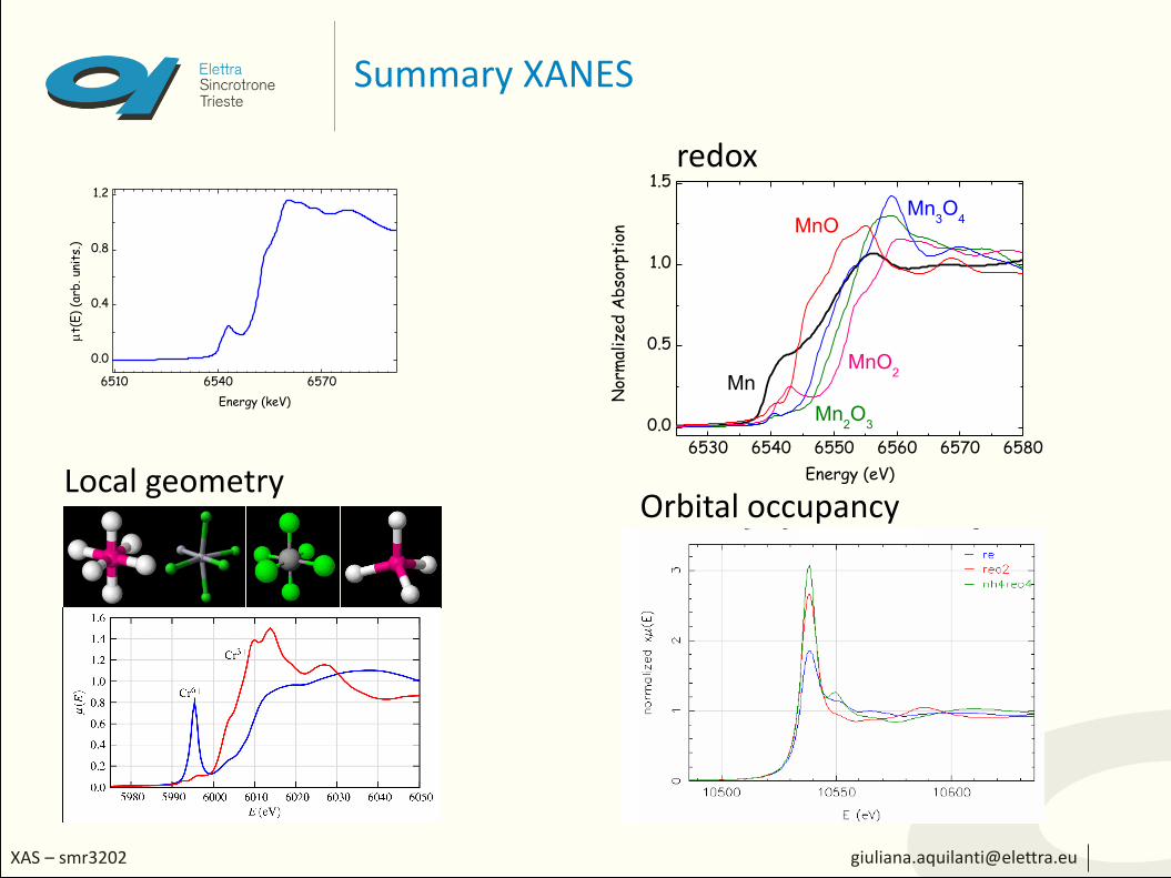
Summary XANES
6510 6540 6570
0.0
0.4
0.8
1.2
mt(
E)
(arb
. un
its.
)
Energy (keV)
6530 6540 6550 6560 6570 6580
0.0
0.5
1.0
1.5
MnMnO
2
Mn2O
3
Mn3O
4
Nor
mal
ized A
bso
rpti
on
Energy (eV)
MnO
redox
Local geometryOrbital occupancy
[email protected] – smr3202
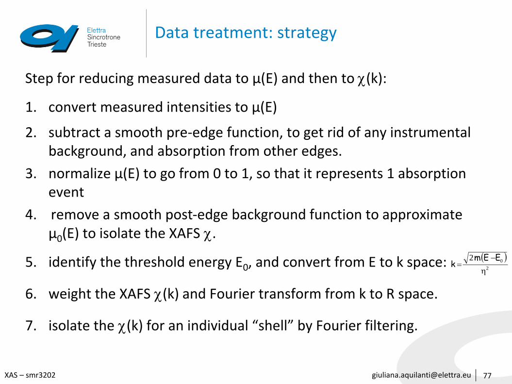
Data treatment: strategy
77
Step for reducing measured data to μ(E) and then to (k):
1. convert measured intensities to μ(E)
2. subtract a smooth pre-edge function, to get rid of any instrumental background, and absorption from other edges.
3. normalize μ(E) to go from 0 to 1, so that it represents 1 absorption event
4. remove a smooth post-edge background function to approximate μ0(E) to isolate the XAFS .
5. identify the threshold energy E0, and convert from E to k space:
6. weight the XAFS (k) and Fourier transform from k to R space.
7. isolate the (k) for an individual “shell” by Fourier filtering.
2
02
EEmk
[email protected] – smr3202
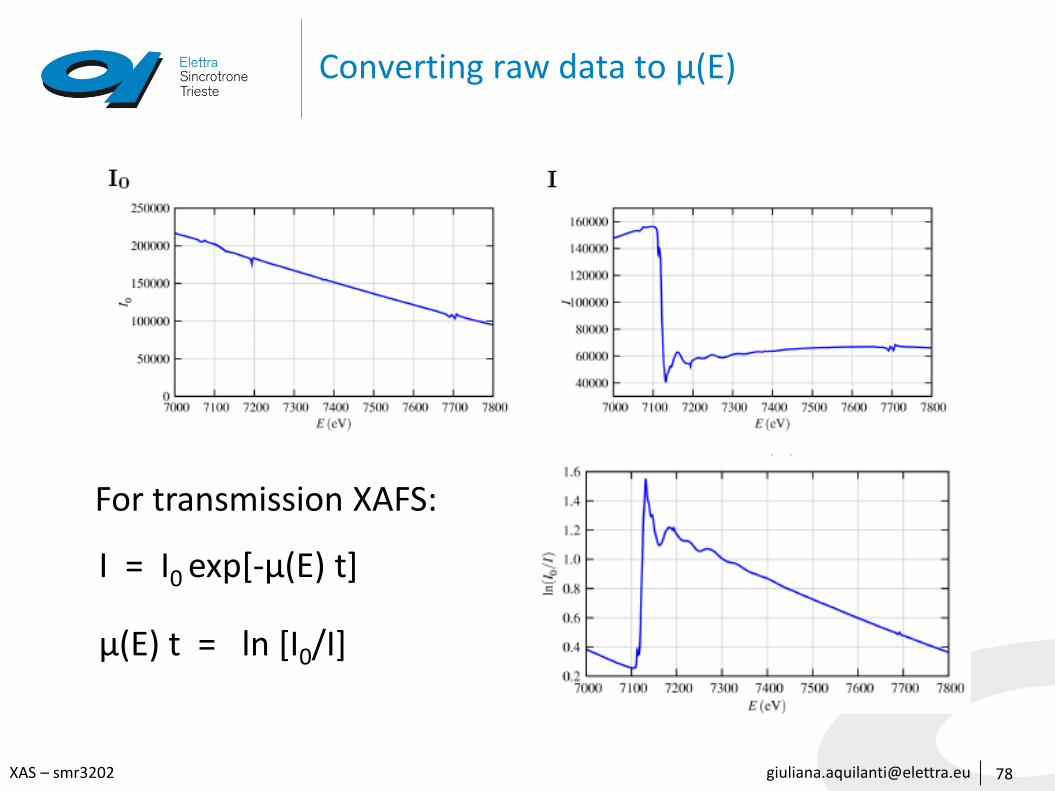
Converting raw data to μ(E)
78
For transmission XAFS:
I = I0 exp[-μ(E) t]
μ(E) t = ln [I0/I]

[email protected] – smr3202
Absorption measurements in real life
79
Transmission
The absorption is measured directly by measuring what is transmitted through the sample
𝐼 = 𝐼0𝑒−𝜇 𝐸 𝑡
𝜇 𝐸 𝑡 = α = ln 𝐼0 𝐼1
Fluorescence
The re-filling the deep core hole is detected. Typically the fluorescent X-ray is measured
𝛼 ∝ 𝐼𝐹 𝐼0
synchrotron source
monochromator sample
I0
IF
I1
[email protected] – smr3202
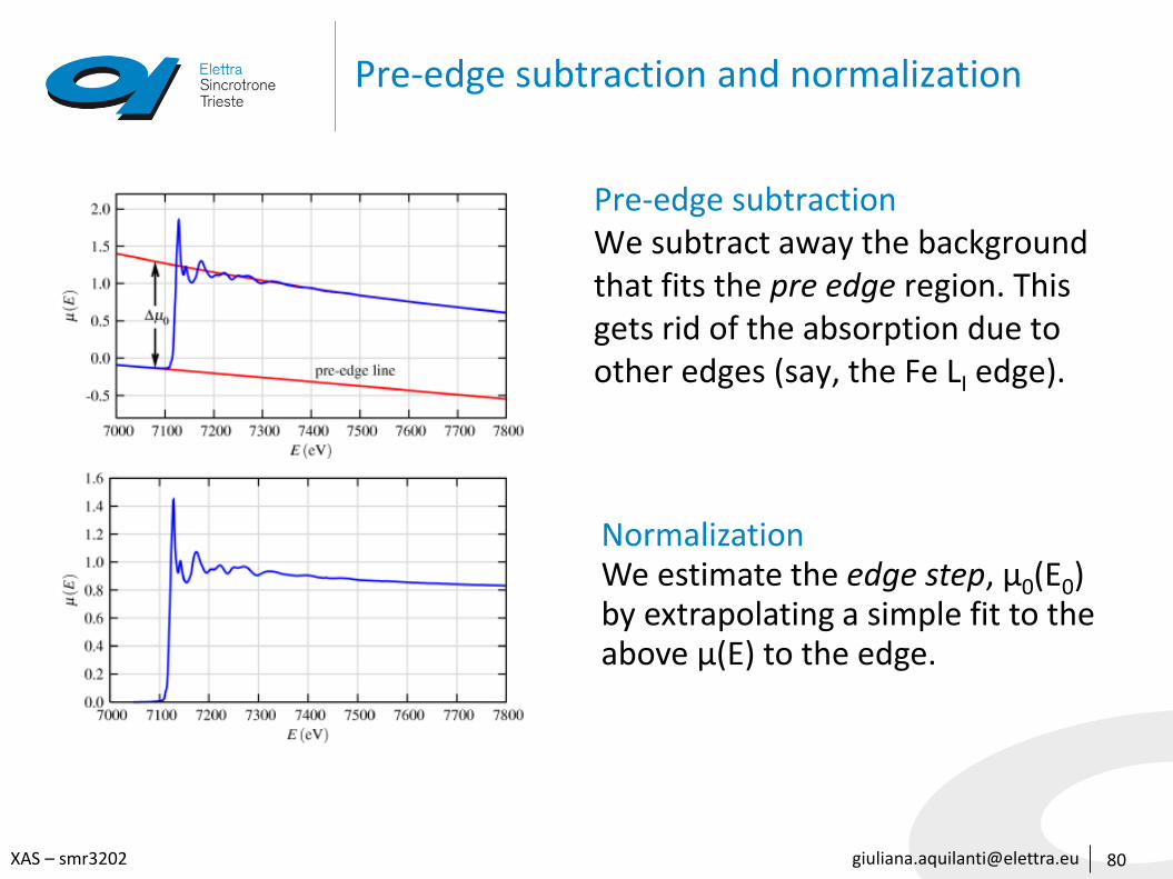
Pre-edge subtraction and normalization
80
Pre-edge subtractionWe subtract away the backgroundthat fits the pre edge region. Thisgets rid of the absorption due toother edges (say, the Fe LI edge).
NormalizationWe estimate the edge step, μ0(E0) by extrapolating a simple fit to the above μ(E) to the edge.
[email protected] – smr3202
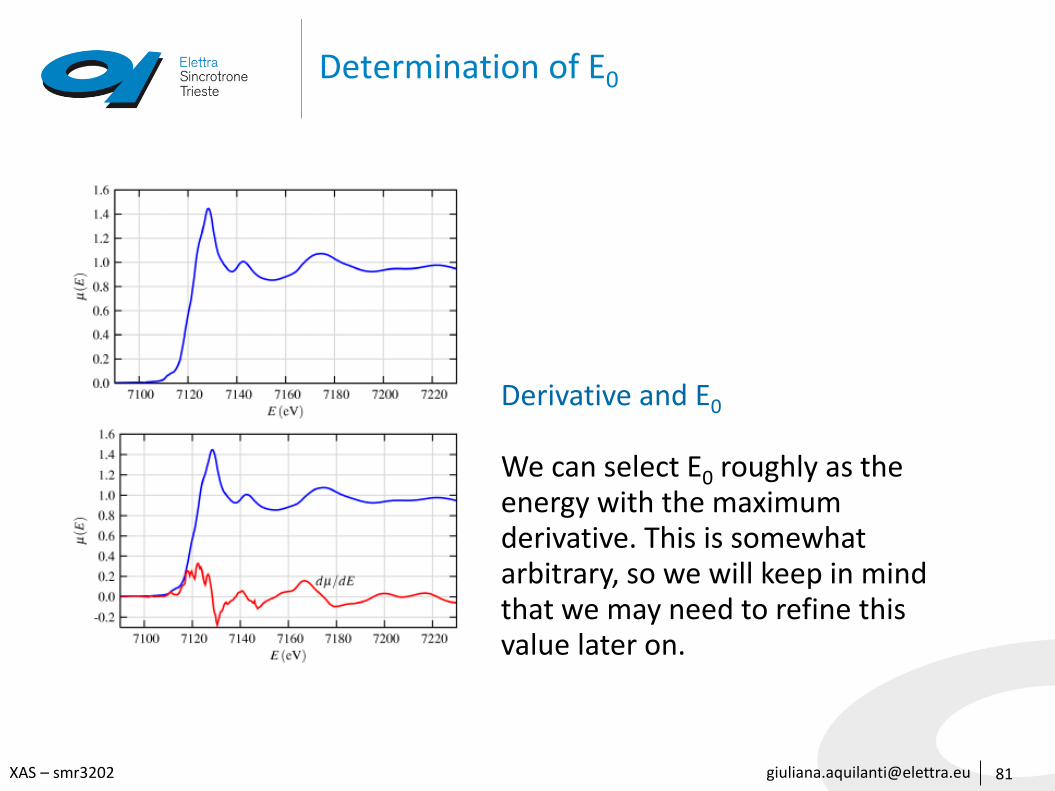
Determination of E0
81
Derivative and E0
We can select E0 roughly as the energy with the maximum derivative. This is somewhat arbitrary, so we will keep in mind that we may need to refine this value later on.
[email protected] – smr3202
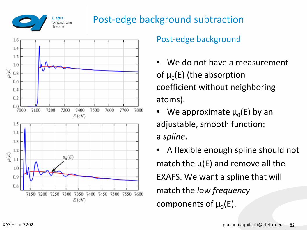
Post-edge background subtraction
82
Post-edge background
• We do not have a measurement
of μ0(E) (the absorption
coefficient without neighboring
atoms).
• We approximate μ0(E) by an
adjustable, smooth function:
a spline.
• A flexible enough spline should not
match the μ(E) and remove all the
EXAFS. We want a spline that will
match the low frequency
components of μ0(E).
[email protected] – smr3202
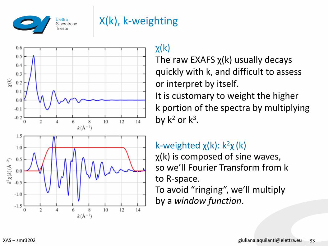
Χ(k), k-weighting
83
χ(k)The raw EXAFS χ(k) usually decaysquickly with k, and difficult to assessor interpret by itself.It is customary to weight the higherk portion of the spectra by multiplyingby k2 or k3.
k-weighted χ(k): k2χ (k)χ(k) is composed of sine waves, so we’ll Fourier Transform from k to R-space. To avoid “ringing”, we’ll multiplyby a window function.
[email protected] – smr3202
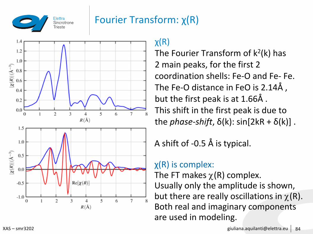
Fourier Transform: χ(R)
84
χ(R)The Fourier Transform of k2(k) has2 main peaks, for the first 2coordination shells: Fe-O and Fe- Fe.The Fe-O distance in FeO is 2.14Å ,but the first peak is at 1.66Å . This shift in the first peak is due tothe phase-shift, δ(k): sin[2kR + δ(k)] .
A shift of -0.5 Å is typical.
χ(R) is complex:The FT makes (R) complex.Usually only the amplitude is shown, but there are really oscillations in (R).Both real and imaginary componentsare used in modeling.
[email protected] – smr3202
Fourier filtering
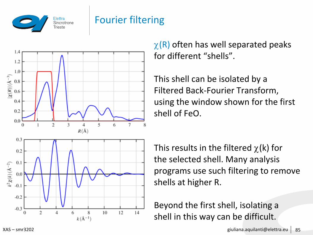
85
(R) often has well separated peaksfor different “shells”.
This shell can be isolated by a Filtered Back-Fourier Transform,using the window shown for the firstshell of FeO.
This results in the filtered (k) forthe selected shell. Many analysisprograms use such filtering to removeshells at higher R.
Beyond the first shell, isolating ashell in this way can be difficult.
[email protected] – smr3202
The information content of EXAFS
86
• The number of parameters we can reliably measure from our data is limited:
where Dk and DR are the k- and R-ranges of the usable data.• For the typical ranges like k = [3.0, 12.0] Å−1 and R = [1.0, 3.0] Å, there
are ~ 11 parameters that can be determined from EXAFS.• The “Goodness of Fit” statistics, and confidence in the measured
parameters need to reflect this limited amount of data.• It is often important to constrain parameters R, N, s2 for different
paths or even different data sets (different edge elements, temperatures, etc)
• Chemical Plausibility can also be incorporated, either to weed out obviously bad results or to use other knowledge of local coordination, such as the Bond Valence Model (relating valence, distance, and coordination number).
• Use as much other information about the system as possible!
RkN
DD
2
[email protected] – smr3202
Modeling the first shell of FeO - 1
87
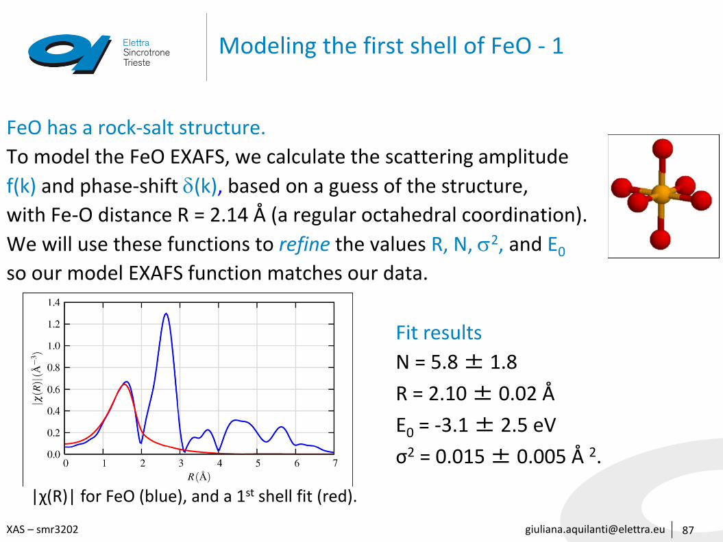
FeO has a rock-salt structure.
To model the FeO EXAFS, we calculate the scattering amplitude
f(k) and phase-shift d(k), based on a guess of the structure,
with Fe-O distance R = 2.14 Å (a regular octahedral coordination).
We will use these functions to refine the values R, N, s2, and E0
so our model EXAFS function matches our data.
Fit results
N = 5.8 ± 1.8
R = 2.10 ± 0.02 Å
E0 = -3.1 ± 2.5 eV
σ2 = 0.015 ± 0.005 Å 2.
|χ(R)| for FeO (blue), and a 1st shell fit (red).
[email protected] – smr3202
Modeling the first shell of FeO - 2
88
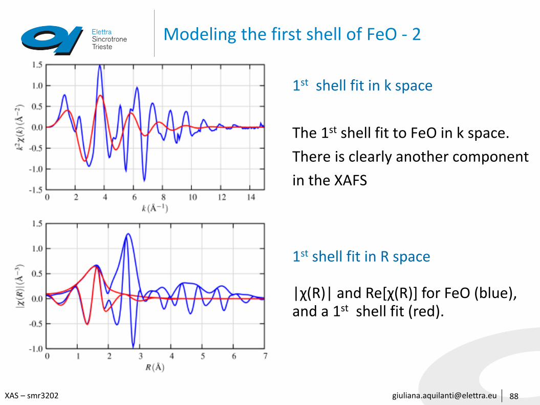
1st shell fit in k space
The 1st shell fit to FeO in k space.
There is clearly another component
in the XAFS
1st shell fit in R space
|χ(R)| and Re[χ(R)] for FeO (blue), and a 1st shell fit (red).
[email protected] – smr3202 89
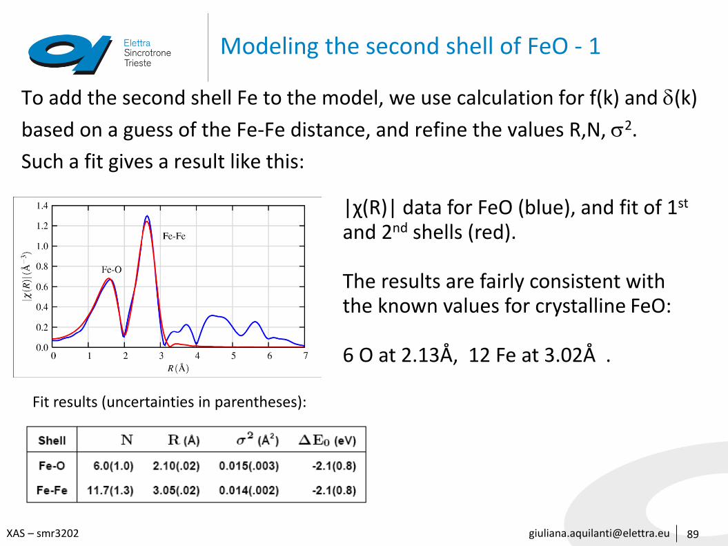
Modeling the second shell of FeO - 1
To add the second shell Fe to the model, we use calculation for f(k) and d(k)
based on a guess of the Fe-Fe distance, and refine the values R,N, s2.
Such a fit gives a result like this:
|χ(R)| data for FeO (blue), and fit of 1st
and 2nd shells (red).
The results are fairly consistent with the known values for crystalline FeO:
6 O at 2.13Å, 12 Fe at 3.02Å .
Fit results (uncertainties in parentheses):
[email protected] – smr3202 90
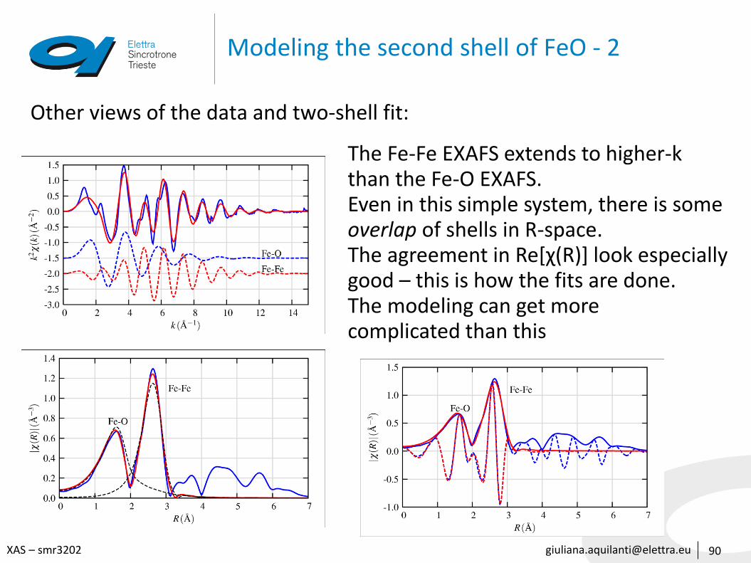
Modeling the second shell of FeO - 2
Other views of the data and two-shell fit:
The Fe-Fe EXAFS extends to higher-kthan the Fe-O EXAFS.Even in this simple system, there is someoverlap of shells in R-space.The agreement in Re[χ(R)] look especially good – this is how the fits are done.The modeling can get morecomplicated than this
[email protected] – smr3202
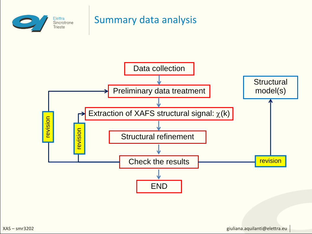
Summary data analysis
Data collection
Extraction of XAFS structural signal: (k)
Structural refinement
Check the results
END
Preliminary data treatmentStructural model(s)
revision
revis
ion
revis
ion


![MURDOCH RESEARCH REPOSITORY...X-ray absorption near-edge structure (XANES) has been previously used to study the structural properties of Al-incorporated titanium nitride [23]. In](https://img.pdfslide.us/doc/110x75/606b4e6d9f2d816a2110f0f8/murdoch-research-repository-x-ray-absorption-near-edge-structure-xanes-has.jpg)