Www.monash.edu.au Clayton School of IT Wireless Network Management Pravin Shetty Monash University Clayton School of IT

www.monash.edu.au Clayton School of IT

Wireless Network Management

Pravin Shetty

Monash University

Clayton School of IT


2

Today’s Lecture

• Why Wireless?

• Overview

• Resources


3


4

Market Size

• Wireless as the common case vs. the exception

– Laptop (54%) vs. desktop sales (46%)

– >2B cell phones vs. 500M Internet-connected PCs

– Estimates of ~5-10B wireless sensors by 2015

• Rapid deployment of new technology

– Highly dynamic environment– Must accommodate

new/unexpected technologies

• 9 million hotspot users in 2003 (30 million in 2004)

• Approx 4.5 million WiFi access points sold in 3Q04

• Sales will triple by 2009• Many more non-802.11 devices

Staggering Market Statistics

7/2004 wardrive (802.11g standardized in 6/2003)

Total 667

Classified 472

802.11b 379

802.11g 93


5

Why is it so popular?

• Flexible• Low cost• Easy to deploy• Support mobility


6

Implication: Market Size

• Past efforts emphasis on adapting wireless nodes to support existing architecture– Wireless TCP, Mobile IP, etc.– Adoption of these evolutionary changes has lagged

expectations

• Market size justifies more dramatic changes– Broader architectural changes to support range of

issues created by wireless systems– Consider changes to Internet that may simplify future

wireless system design


7

Growing Deployment Diversity

Devices

Laptops, PDAs, audio/video equipment, appliances, sensors and “Constellations” of devices

Scale

Billions of sensors & RFID tags expected by 2015

Deployment styles

Homes, hot-spots, airports and infrastructure/municipal networks

• Past: largely 802.11 campus networks with laptops

FUTURE

Radio technology

Sensor radios, 3+G cellular, Bluetooth, UWB, WiMax, software radios, and RFID


8

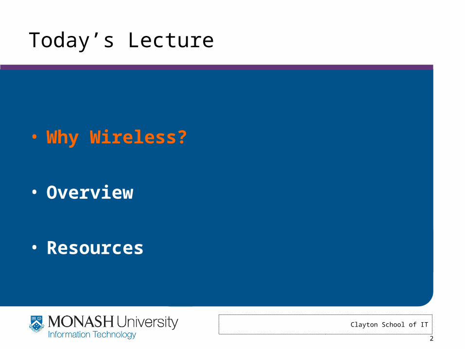
Wireless Technologies

UWB

Bluetooth

WiFi

3G

range

BW

WiMax

RFID


9


10


11

Spectrum Scarcity

Portland 8683 54

San Diego 7934 76

San Fran 3037 85

Boston 2551 39

#APs Max @ 1 spot

• Densities of unlicensed devices already high

• Spectrum is scarce will get worse

– Improve spectrum utilization (currently 10%)


12

Spectrum Scarcity

• Interference and unpredictable behavior– Need better management/diagnosis tools

• Lack of isolation between deployments– Cross-domain and cross-technology

Why is my 802.11 not working?


13

Wireless Differences 1

• Physical layer: signals travel in open space

• Subject to interference– From other sources and self (multipath)

• Creates interference for other wireless devices

• Noisy lots of losses• Channel conditions can be very dynamic


14


• Need to share airwaves rather than wire

• Don’t know what hosts are involved• Hosts may not be using same link technology• Interaction of multiple transmitters at receiver

– Collisions, capture, interference• Use of spectrum: limited resource.

– Cannot “create” more capacity very easily– More pressure to use spectrum efficiently


15


• Mobility– Must update routing protocols to handle frequent

changes> Requires hand off as mobile host moves in/out range

– Changes in the channel conditions.> Coarse time scale: distance/interference/obstacles

change> Fine time scale: Doppler effect

• Other characteristics of wireless– Slow


16

Wireless Networking

1980’s 1990’s 2000’s

1G Cellular Telephony

Technology

Research Goals

2G Digital Cellular

First Generation

Wireless LANs

3G Data-oriented Cellular

802.11 LANs

Invisible computing, sensors

Focus on HCI, integration, low power

Ubiquitous access to data

Challenges: coverage, speed, disconnected operation, devices, ad hoc

Applications, hardware, networking (PARC, Infopad, BARWAN, Odyssey, etc.)


17

Device Diversity – Network Interfaces Design

1990’s 2000’s 2010’s

Single wireless interface per machine

• Initially developed in mid 90’s• Require high-bandwidth I/O & lots

of processing• Couldn’t easily handle low-latency

interaction required by modern link standards

• Still power hungry

Multiple interfaces per machine

Software defined radios?Directional antennas?


18

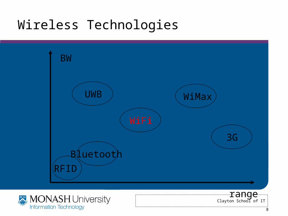
Overview

• Physical layer Textbook-based– Signal encoding/modulation– Signal propagation basics– Spread spectrum concepts– Public policy

• Link layer– 802.11– Emerging technologies (Bluetooth, WiMax, etc.)– Wireless MAC protocols– Software Radios


19

Overview

• Multi-hop networks– Ad hoc routing

– Network capacity

– Routing metrics

– Mesh networks

– Geographic routing


20

Overview

• Applications layer– Disconnected operation– Adaptive applications– Delay tolerant networking– Localization

• Miscellaneous Network simulation/testbeds– Multi radio networks– Mobile IP connectivity– Wireless TCP– Security– Wireless network management


24

Network Protocols

• Protocol– A set of rules and formats that govern the

communication between communicating peers

• Protocol layering– Decompose a complex problem into smaller

manageable pieces (e.g., Web server)– Abstraction of implementation details– Reuse functionality– Ease maintenance– Cons?


25

Network Protocol Stack

• Application: supporting network applications– FTP, SMTP, HTTP

• Transport: host-host data transfer– TCP, UDP

• Network: routing of datagrams from source to destination– IP, routing protocols

• Link: data transfer between neighboring network elements– WiFi, Ethernet

• Physical: bits “on the wire”– Radios, coaxial cable, optical fibers

application

transport

network

link

physical


26

From Signals to Packets

Analog Signal

“Digital” Signal

Bit Stream 0 0 1 0 1 1 1 0 0 0 1

Packets0100010101011100101010101011101110000001111010101110101010101101011010111001

Header/Body Header/Body Header/Body

ReceiverSenderPacket

Transmission


27

Outline

• RF introduction– What is “RF”– Digital versus analog contents

• Modulation• Antennas and signal propagation• Equalization, diversity, channel coding• Multiple access techniques• Wireless systems and standards


28

RF Introduction

• RF = Radio Frequency.– Electromagnetic signal that propagates through “ether”– Ranges 3 KHz .. 300 GHz– Or 10 km .. 0.1 cm (wavelength)

• Has been used for communication for a long time, but improvements in technology have made it possible to use higher frequencies.


29

Wireless Communication

• 300 GHz is huge amount of spectrum!– Spectrum can also be reused in space

• Not quite that easy:– Most of it is hard or expensive to use!– Noise and interference limits efficiency– Most of the spectrum is allocated by FCC

• FCC controls who can use the spectrum and how it can be used.

– Need a license for most of the spectrum– Limits on power, placement of transmitters, coding, ..– Need rules to optimize benefit: guarantee emergency

services, simplify communication, return on capital investment, …


30

Spectrum Allocation

See: http://www.ntia.doc.gov/osmhome/allochrt.html

Most bands are allocated.• Industrial, Scientific, and Medical (ISM) bands are

“unlicensed”.– But still subject to various constraints on the operator,

e.g. 1 W output– 433-868 MHz (Europe)– 902-928 MHz (US)– 2.4000-2.4835 GHz– Unlicensed National Information Infrastructure (UNII)

band is 5.725-5.875 GHz


31

What Is an Electromagnetic Signal

• We will be vague about this and we will use two “cartoon” views:

• Think of it as energy that radiates from an antenna and is picked up by another antenna.– Can easily explain properties such as attenuation

• Can also view it as a “wave” that propagates between two points.– Can easily explain properties

Space and Time


32

Decibels

• A ratio between signal powers is expressed in decibelsdecibels (db) = 10log10(P1 / P2)

• Is used in many contexts:– The loss of a wireless channel– The gain of an amplifier

• Note that dB is a relative value.• Can be made absolute by picking a reference point.

– Decibel-Watt – power relative to 1W– Decibel-milliwatt – power relative to 1 milliwatt

> 4.5 mW = (10*log10 4.5) dBm


33

Analog and Digital Information

• Initial RF use was for analog information.– Radio and TV stations– The information that is sent is of a continuous nature

• In digital transmission, the signal consists of discrete units (e.g. bits).

– Data networks, cell phones– Focus of this course

• We can also send analog information as digital data.– Sample the signal, i.e. analog digital analog

> E.g., Cell phones, …– Also digital analog digital (e.g. modem)


34

Outline

• RF introduction• Modulation

– Baseband versus carrier modulation

– Forms of modulation

– Channel capacity

• Antennas and signal propagation• Equalization, diversity, channel coding• Multiple access techniques• Wireless systems and standards


35

The Frequency Domain

• A (periodic) signal can be viewed as a sum of sine waves of different strengths.

– Corresponds to energy at a certain frequency• Every signal has an equivalent representation in the frequency

domain.– What frequencies are present and what is their strength (energy)

• Again: Similar to radio and TV signals.

TimeFrequency

Am

plit

ude


36

Signal = Sum of Sine Waves

=

+ 1.3 X

+ 0.56 X

+ 1.15 X


37

Modulation

• Sender changes the nature of the signal in a way that the receiver can recognize.

– Assume a continuous information signal for now

• Amplitude modulation (AM): change the strength of the carrier according to the information.

– High values stronger signal

• Frequency (FM) and phase modulation (PM): change the frequency or phase of the signal.

– Frequency or Phase shift keying

• Digital versions are sometimes called “shift keying”.– Amplitude (ASK), Frequency (FSK) and Phase (PSK) Shift

Keying


38

Baseband versus Carrier Modulation

• Baseband modulation: send the “bare” signal.– Use the lower part of the spectrum– Everybody competes – not attractive for wireless

• Carrier modulation: use the (information) signal to modulate a higher frequency (carrier) signal.

– Can be viewed as the product of the two signals– Corresponds to a shift in the frequency domain


39

Frequency Division Multiplexing:Multiple Channels

Am

plitu

de

Different CarrierFrequencies

DeterminesBandwidthof Channel

Determines Bandwidth of Link


40

Signal Bandwidth Considerations

• The more frequencies are present in a signal, the more detail can be represented in the signal.

– The signal can look “cleaner”

– Energy is distributed over a larger part of the spectrum, i.e. it consumes more (spectrum) bandwidth

• Signals with more detail can represent more bits, so in general, higher (spectrum) bandwidth translates into a higher (information) bandwidth.


41

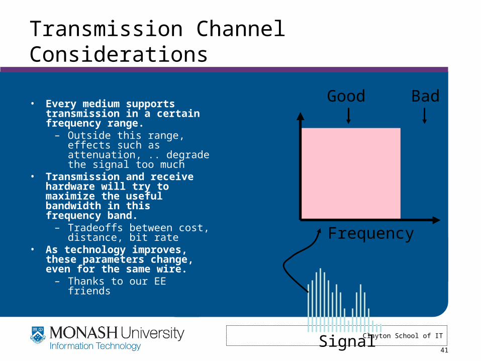
Transmission Channel Considerations

• Every medium supports transmission in a certain frequency range.

– Outside this range, effects such as attenuation, .. degrade the signal too much

• Transmission and receive hardware will try to maximize the useful bandwidth in this frequency band.

– Tradeoffs between cost, distance, bit rate

• As technology improves, these parameters change, even for the same wire.

– Thanks to our EE friends

Frequency

Good Bad

Signal


42

The Nyquist Limit

• A noiseless channel of width H can at most transmit a binary signal at a rate 2 x H.

– E.g. a 3000 Hz channel can transmit data at a rate of at most 6000 bits/second

– Assumes binary amplitude encoding


43

Past the Nyquist Limit

• More aggressive encoding can increase the channel bandwidth.

– Example: modems> Same frequency - number of symbols per second> Symbols have more possible values

pskPsk+ AM


45

Some Examples

• Differential quadrature phase shift keying– Four different phases representing a pair of bits

– Used in 802.11b networks

• Quadrature Amplitude Modulation– Combines amplitude and phase modulation

– Uses two amplitudes and 4 phases to represent the value of a 3 bit sequence


46

Modulation vs. BER

• More symbols =– Higher data rate: More information per baud– Higher bit error rate: Harder to distinguish symbols

• Why useful?– 802.11b uses DBPSK (differential binary phase shift keying)

for 1Mbps, and DQPSK (quadriture) for 2, 5.5, and 11. – 802.11a uses four schemes - BPSK, PSK, 16-QAM, and 64-

AM, as its rates go higher.• Effect: If your BER / packet loss rate is too high, drop down

the speed: more noise resistance.• We’ll see in some papers later in the semester that this means

noise resistance isn’t always linear with speed.


47

Outline

• RF introduction• Modulation• Antennas and signal propagation

– How do antennas work– Propagation properties of RF signals

• Equalization, diversity, channel coding• Multiple access techniques• Wireless systems and standards


48

What is an Antenna?

• Conductor that carries an electrical signal and radiates an RF signal.– The RF signal “is a copy of” the electrical signal in the

conductor• Also the inverse process: RF signals are

“captured” by the antenna and create an electrical signal in the conductor.– This signal can be interpreted (i.e. decoded)

• Efficiency of the antenna depends on its size, relative to the wavelength of the signal.– E.g. half a wavelength


49

Types of Antennas

• Abstract view: antenna is a point source that radiates with the same power level in all directions – omni-directional or isotropic.– Not common – shape of the conductor tends to create

a specific radiation pattern– Note that isotropic antennas are not very efficient!!

> Unless you have a very large number of receivers

• Shaped antennas can be used to direct the energy in a certain direction.– Well-known case: a parabolic antenna– Pringles boxes are cheaper


50

Antennas and Attenuation

• Isotropic Radiator: A theoretical antenna– Perfectly spherical radiation.– Used for reference and FCC regulations.

• Dipole antenna (vertical wire)– Radiation pattern like a doughnut

• Parabolic antenna– Radiation pattern like a long balloon

• Yagi antenna (common in 802.11)– Looks like |--|--|--|--|--|--|– Directional, pretty much like a parabolic reflector


51

Directional Antenna Properties

• dBi: antenna gain in dB relative to an isotropic antenna with the same power.

– Example: an 8 dBi Yagi antenna has a gain of a factor of 6.3 (8 db = 10 log 6.3)


52

Antennas

• Spatial reuse:– Directional antennas allow more communication in same 3D

space• Gain:

– Focus RF energy in a certain direction– Works for both transmission and reception

• Frequency specific– Frequency range dependant on length / design of antenna,

relative to wavelength.• FCC bit: Effective Isotropic Radiated Power. (EIRP).

– Favors directionality. E.g., you can use an 8dB gain antenna b/c of spatial characteristics, but not always an 8dB amplifier.


53

Propagation Modes

• Line-of-sight (LOS) propagation.– Most common form of propagation– Happens above ~ 30 MHz– Subject to many forms of degradation (next set of slides)

• Ground-wave propagation.– More or less follows the contour of the earth– For frequencies up to about 2 MHz, e.g. AM radio

• Sky wave propagation.– Signal “bounces” off the ionosphere back to earth – can

go multiple hops– Used for amateur radio and international broadcasts


54

Limits to Speed and Distance

• Noise: “random” energy is added to the signal

• Attenuation: some of the energy in the signal leaks away

• Dispersion: attenuation and propagation speed are frequency dependent.

– Changes the shape of the signal


55

Propagation Degrades RF Signals

• Attenuation in free space: signal gets weaker as it travels over longer distances.

– Radio signal spreads out – free space loss– Absorption

• Obstacles can weaken signal through absorption or reflection.– Part of the signal is redirected

• Multi-path effects: multiple copies of the signal interfere with each other.

– Similar to an unplanned directional antenna• Mobility: moving receiver causes another form of self

interference.– Receiver moves ½ wavelength -> big change in wavelength


56

Refraction

• Speed of EM signals depends on the density of the material.

– Vacuum: 3 x 108 m/sec– Denser: slower

• Density is captured by refractive index.

• Explains “bending” of signals in some environments.

– E.g. sky wave propagation– But also local, small scale

differences in the air

denser


57

Other LOS Factors

• There are many noise sources.– Thermal noise: caused by agitation of the electrons– Intermodulation noise: result of mixing signals;

appears at f1 + f2 and f1 – f2

– Cross talk: picking up other signals (i.e. from other source-destination pairs)

– Impulse noise: irregular pulses of high amplitude and short duration – harder to deal with

• Absorption of energy in the atmosphere.– Very serious at specific frequencies, e.g. water

vapor (22 GHz) and oxygen (60 GHz)– Obviously objects also absorb

FairlyPredictableCan be planned foror avoided


58

Propagation Mechanisms

• Besides line of sight, signal can reach receiver in three other “indirect” ways.

• Reflection: signal is reflected from a large object.

• Diffraction: signal is scattered by the edge of a large object – “bends”.

• Scattering: signal is scattered by an object that is small relative to the wavelength.


59


60

Example


62

Fading in the Mobile Environment

• Fading: time variation of the received signal strength caused by changes in the transmission medium or paths.

– Rain, moving objects, moving sender/receiver, …• Fast versus slow fading.

– Fast: changes in distance of about half a wavelength – result in big fluctuations in the instantaneous power

– Slow: changes in larger distances affects the paths – result in a change in the average power levels around which the fast fading takes place

• Selective versus non-selective (flat) fading.– Does the fading affect all frequency components equally– Region of interest is the spectrum used by the channel


63

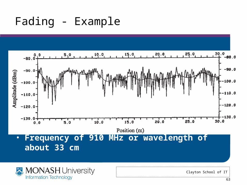
Fading - Example

• Frequency of 910 MHz or wavelength of about 33 cm


64

Wireless Technologies

• Great technology: no wires to install, convenient mobility, ..

• High attenuation limits distances.– Wave propagates out as a sphere– Signal strength reduces quickly (1/distance)3

• High noise due to interference from other transmitters.– Use MAC and other rules to limit interference– Aggressive encoding techniques to make signal less

sensitive to noise• Other effects: multipath fading, security, ..• Ether has limited bandwidth.

– Try to maximize its use– Government oversight to control use


65

Medium Access Control

• Think back to Ethernet MAC:– Wireless is a shared medium– Transmitters interfere– Need a way to ensure that (usually) only one person talks

at a time.> Goals: Efficiency, possibly fairness

• But wireless is harder!– Can’t really do collision detection:

> Can’t listen while you’re transmitting. You overwhelm your antenna…

– Carrier sense is a bit weaker:> Takes a while to switch between Tx/Rx.

– Wireless is not perfectly broadcast


66

“Wireless Ethernet”

• Collision detection is not practical.– Signal power is too high at the transmitter– So how do you detect collisions?

• Signals attenuate significantly with distance.– Strong signal from nearby node will overwhelm the weaker

signal from a remote transmitter– Capture effect: nearby node will always win in case of collision -

receiver may not even detect remote node> Hidden transmitter

• Two transmitters may not hear each other, which can cause collisions at a common receiver.

– Hidden terminal problem– RTS/CTS is designed to avoid this


67

A B C

Hidden Terminal Problem

• B can communicate with both A and C• A and C cannot hear each other• Problem

– When A transmits to B, C cannot detect the transmission using the carrier sense mechanism

– If C transmits, collision will occur at node B• Solution

– Hidden sender C needs to defer


68

802.11 RTS/CTS

• RTS sets “duration” field in header to– CTS time + SIFS + CTS time + SIFS + data

pkt time• Receiver responds with a CTS

– Field also known as the “NAV” - network allocation vector

– Duration set to RTS dur - CTS/SIFS time– This reserves the medium for people who

hear the CTS


69

Medium Access Control

• Think back to Ethernet MAC:– Wireless is a shared medium– Transmitters interfere– Need a way to ensure that (usually) only one person talks

at a time.> Goals: Efficiency, possibly fairness

• But wireless is harder!– Can’t really do collision detection:

> Can’t listen while you’re transmitting. You overwhelm your antenna…

– Carrier sense is a bit weaker:> Takes a while to switch between Tx/Rx.

– Wireless is not perfectly broadcast


70

C FA B EDRTS

RTS = Request-to-Send

IEEE 802.11

assuming a circular range


71

C FA B EDRTS

RTS = Request-to-Send

IEEE 802.11

NAV = 10

NAV = remaining duration to keep quiet


72

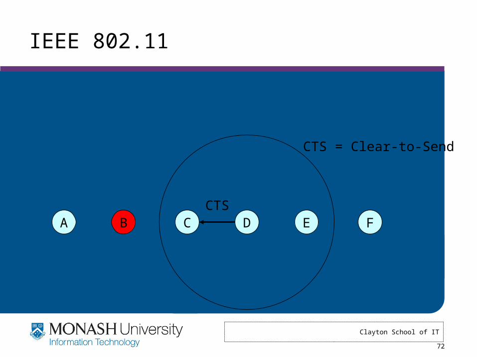
C FA B EDCTS

CTS = Clear-to-Send

IEEE 802.11


73

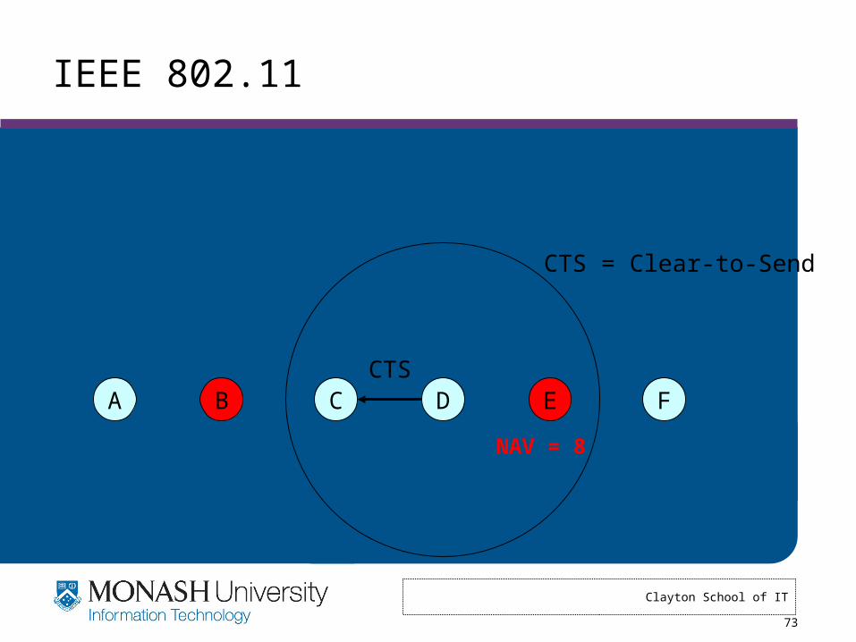
C FA B EDCTS

CTS = Clear-to-Send

IEEE 802.11

NAV = 8


74

C FA B EDDATA

•DATA packet follows CTS. Successful data reception acknowledged using ACK.

IEEE 802.11


75

IEEE 802.11

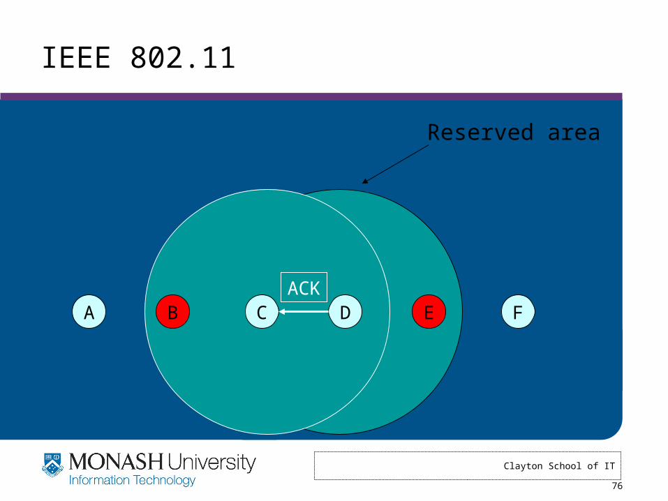
C FA B EDACK


76

C FA B EDACK

IEEE 802.11

Reserved area


77

IEEE 802.11

C FA B EDDATA

Transmit “range”

Interference“range”

Carrier senserange

FA


78

IEEE 802.11 Overview

• Adopted in 1997

Defines:• MAC sublayer • MAC management protocols and services• Physical (PHY) layers

– IR

– FHSS

– DSSS


79

802.11 particulars

• 802.11b (WiFi)– Frequency: 2.4 - 2.4835 Ghz DSSS

– Modulation: DBPSK (1Mbps) / DQPSK (faster)

– Orthogonal channels: 3> There are others, but they interfere. (!)

– Rates: 1, 2, 5.5, 11 Mbps

• 802.11a: Faster, 5Ghz OFDM. Up to 54Mbps• 802.11g: Faster, 2.4Ghz, up to 54Mbps


80

802.11 details

• Fragmentation– 802.11 can fragment large packets (this is separate

from IP fragmentation).• Preamble

– 72 bits @ 1Mbps, 48 bits @ 2Mbps– Note the relatively high per-packet overhead.

• Control frames– RTS/CTS/ACK/etc.

• Management frames– Association request, beacons, authentication, etc.


81

Overview, 802.11 Architecture

STASTA

STA STA

STASTASTA STA

APAP

ESS

BSS

BSSBSS

BSS

Existing Wired LAN

Infrastructure Network

Ad Hoc Network

Ad Hoc Network

BSS: Basic Service SetESS: Extended Service Set


82

802.11 modes

• Infrastructure mode– All packets go through a base station– Cards associate with a BSS (basic service set)– Multiple BSSs can be linked into an Extended Service

Set (ESS)> Handoff to new BSS in ESS is pretty quick

– Wandering around CMU> Moving to new ESS is slower, may require re-addressing

– Wandering from CMU to Pitt

• Ad Hoc mode– Cards communicate directly.– Perform some, but not all, of the AP functions


84

802.11 Management Operations

• Scanning• Association/Reassociation• Time synchronization• Power management


85

Scanning & Joining

• Goal: find networks in the area

• Passive scanning– No require transmission saves power– Move to each channel, and listen for Beacon frames

• Active scanning– Requires transmission saves time– Move to each channel, and send Probe Request frames to solicit

Probe Responses from a network

• Joining a BSS– Synchronization in TSF and frequency : Adopt PHY parameters :

The BSSID : WEP : Beacon Period : DTIM


86

Association in 802.11

AP

1: Association request

2: Association response

3: Data trafficClient


87

Reassociation in 802.11

New AP

1: Reassociation request

3: Reassociation response

5: Send buffered frames

Old AP

2: verifypreviousassociation

4: sendbufferedframes

Client6: Data traffic


88

Time Synchronization in 802.11

• Timing synchronization function (TSF)– AP controls timing in infrastructure networks

– All stations maintain a local timer

– TSF keeps timer from all stations in sync

• Periodic Beacons convey timing– Beacons are sent at well known intervals

– Timestamp from Beacons used to calibrate local clocks

– Local TSF timer mitigates loss of Beacons


89

Power Management in 802.11

• A station is in one of the three states– Transmitter on– Receiver on– Both transmitter and receiver off (dozing)

• AP buffers packets for dozing stations• AP announces which stations have frames

buffered in its Beacon frames• Dozing stations wake up to listen to the beacons• If there is data buffered for it, it sends a poll

frame to get the buffered data


90

Challenge #1: Wireless Bit-Errors

Router

Computer 2Computer 1

2322

Loss Congestion

21 0

Burst losses lead to coarse-grained timeoutsResult: Low throughput

Loss Congestion

Wireless


91

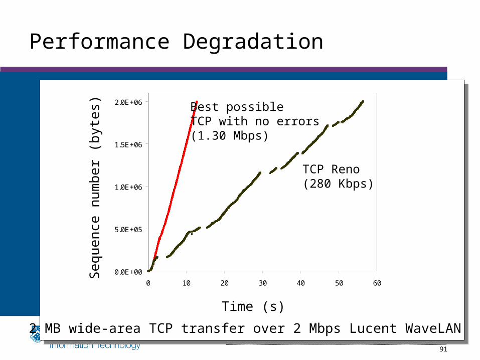
Performance Degradation

0.0E+00

5.0E+05

1.0E+06

1.5E+06

2.0E+06

0 10 20 30 40 50 60

Time (s)

Se

que

nce

nu

mb

er

(byt

es)

TCP Reno(280 Kbps)

Best possible TCP with no errors(1.30 Mbps)

2 MB wide-area TCP transfer over 2 Mbps Lucent WaveLAN


92

Constraints & Requirements

• Incremental deployment– Solution should not require modifications to

fixed hosts

– If possible, avoid modifying mobile hosts

• Probably more data to mobile than from mobile– Attempt to solve this first


93

Proposed Solutions

• End-to-end protocols– Selective ACKs, Explicit loss notification

• Split-connection protocols– Separate connections for wired path and

wireless hop

• Reliable link-layer protocols– Error-correcting codes

– Local retransmission


94

Approach Styles (End-to-End)

• Improve TCP implementations– Not incrementally deployable– Improve loss recovery (SACK, NewReno)– Help it identify congestion (ELN [R.4], ECN)

> ACKs include flag indicating wireless loss– Trick TCP into doing right thing E.g. send extra dupacks

[R.1]

Wired link Wireless link


95

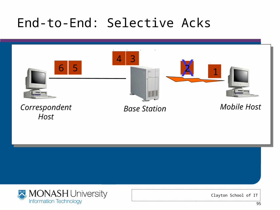
End-to-End: Selective Acks

Correspondent Host

Mobile HostBase Station

5 134

6 X2


96

End-to-End: Selective Acks

Correspondent Host

Mobile HostBase Station

ack 1 ack 1,3 ack 1,3-4 ack 1,3-5 ack 1,3-6


97

Approach Styles (Split Connection)

• Split connections [R.3]– Wireless connection need not be TCP– Hard state at base station

> Complicates mobility> Vulnerable to failures> Violates end-to-end semantics

Wired link Wireless link


98


99

Split-Connection Congestion Window

• Wired connection does not shrink congestion window • But wireless connection times out often, causing sender to stall

0

10000

20000

30000

40000

50000

60000

0 20 40 60 80 100 120

Time (sec)

Con

gest

ion

Win

dow

(by

tes)

Wired connectionWireless connection


100

Approach Styles (Link Layer)

• More aggressive local rexmit than TCP– Bandwidth not wasted on wired links

• Adverse interactions with transport layer– Timer interactions– Interactions with fast retransmissions– Large end-to-end round-trip time variation

• FEC does not work well with burst lossesWired link Wireless link

ARQ/FEC


101

Hybrid Approach: Snoop Protocol

• Described in [R.2]• Transport-aware link protocol• Modify base station

– To cache un-acked TCP packets

– … And perform local retransmissions

• Key ideas– No transport level code in base station

– When node moves to different base station, state eventually recreated there


102

Some Commercial Solutions


103



104



105



106



107

Resources URLS

• AirWave Management Platform (AMP)• http://www.airwave.com/products/AMP_tech.html• Cisco Wireless Location Appliance• http://www.cisco.com/en/US/products/ps6386/products_data_

sheet0900aecd80293728.html• Cisco Wireless Control System• http://www.cisco.com/en/US/products/ps6305/products_data_

sheet0900aecd802570d0.html• ORiNOCO Smart Wireless Suite• http://www.proxim.com/products/sws/


108

Educational resources

• CMU CS15-849E Wireless Networks.– http://www.cs.cmu.edu/~srini/15-849E/S06/

• Recommended textbooks– Wireless Communications & Networks by William

Stallings

Documents

Www.monash.edu.au Clayton School of IT Wireless Network Management Pravin Shetty Monash University Clayton School of IT