Embed Size (px)
Citation preview

1www.izmirekonomi.edu.trMahmut Mahmut Ali GökçeAli Gökçe
Introduction to System Engineering ISE 102 Spring 2007Notes & Course Materials
Asst. Prof. Dr. Mahmut Ali GOKCE
ISE Dept. Faculty of Computer Sciences

www.izmirekonomi.edu.trMahmut Ali GökçeMahmut Ali Gökçe
This Lecture
Review of Week 1 Productivity Modelling Forecasting
www.izmirekonomi.edu.trMahmut Ali GökçeMahmut Ali Gökçe
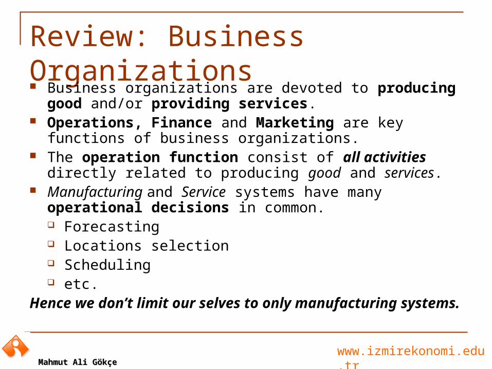
Review: Business Organizations Business organizations are devoted to producing good and/or
providing services. Operations, Finance and Marketing are key functions of
business organizations. The operation function consist of all activities directly related
to producing good and services. Manufacturing and Service systems have many operational
decisions in common. Forecasting Locations selection Scheduling etc.
Hence we don’t limit our selves to only manufacturing systems.

www.izmirekonomi.edu.trMahmut Ali GökçeMahmut Ali Gökçe
Our Job
The design, operation, and improvement of the production systems that create the firm’s products or services.
www.izmirekonomi.edu.trMahmut Ali GökçeMahmut Ali Gökçe
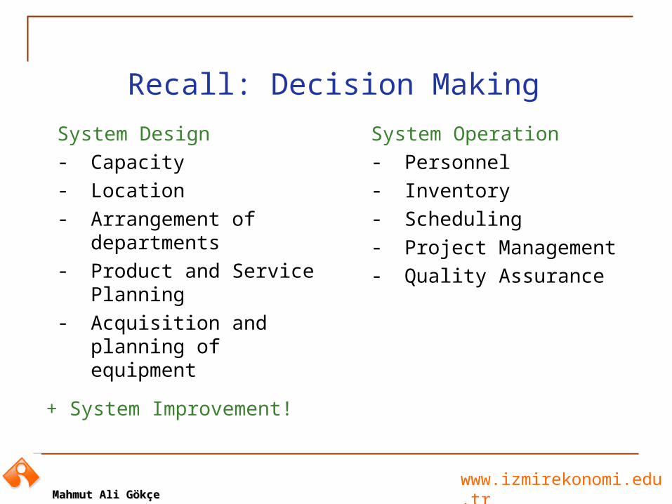
Recall: Decision Making
System Design- Capacity- Location- Arrangement of
departments- Product and Service
Planning- Acquisition and planning
of equipment
System Operation- Personnel- Inventory- Scheduling- Project Management- Quality Assurance
+ System Improvement!
www.izmirekonomi.edu.trMahmut Ali GökçeMahmut Ali Gökçe
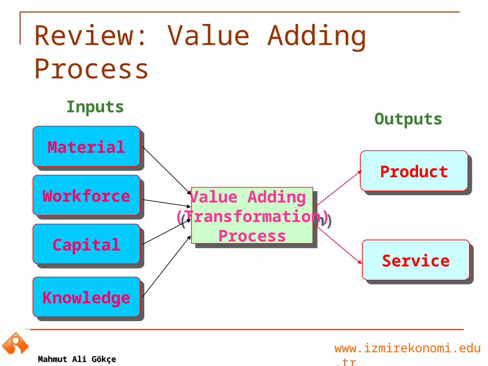
Review: Value Adding Process
Value Adding (Transformation)
Process
Value Adding (Transformation)
Process
ProductProduct
ServiceService
WorkforceWorkforce
KnowledgeKnowledge
CapitalCapital
MaterialMaterial
InputsOutputs
www.izmirekonomi.edu.trMahmut Ali GökçeMahmut Ali Gökçe
Added Value at Operational Level
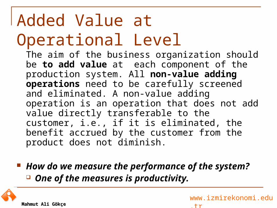
The aim of the business organization should be to add value at each component of the production system. All non-value adding operations need to be carefully screened and eliminated. A non-value adding operation is an operation that does not add value directly transferable to the customer, i.e., if it is eliminated, the benefit accrued by the customer from the product does not diminish.
How do we measure the performance of the system? One of the measures is productivity.

www.izmirekonomi.edu.trMahmut Ali GökçeMahmut Ali Gökçe
Some Definitions: Productivity
Productivity is a measure of the effective use of resources, defined as the ratio of output to input.
Kinds of Productivity: Factor productivity (output is related to one or more
of the resources of production, such as labour, capital, land, raw material, etc.)
Total factor productivity (an overall measure expressing the contribution of the resources of production to the efficiency attained by a firm.)
Both types of productivity can be expressed as physical productivity with output being measured in physical units and as well as value productivity with output being measured in monetary units.
www.izmirekonomi.edu.trMahmut Ali GökçeMahmut Ali Gökçe
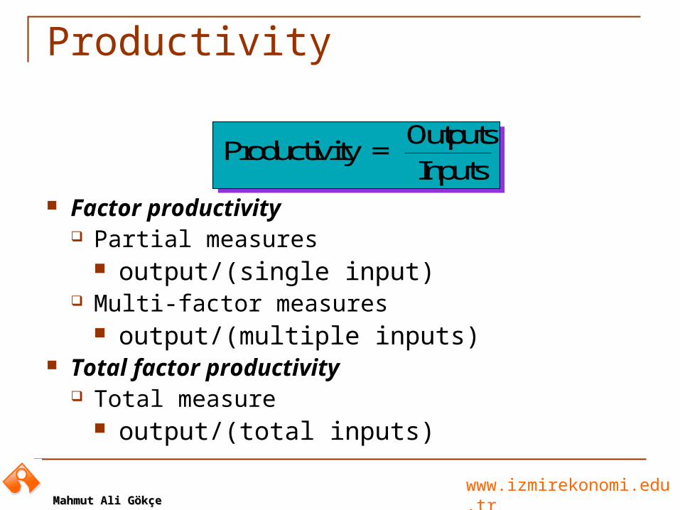
Productivity
Factor productivity Partial measures
output/(single input) Multi-factor measures
output/(multiple inputs) Total factor productivity
Total measure output/(total inputs)
Productivity = Outputs
Inputs
www.izmirekonomi.edu.trMahmut Ali GökçeMahmut Ali Gökçe
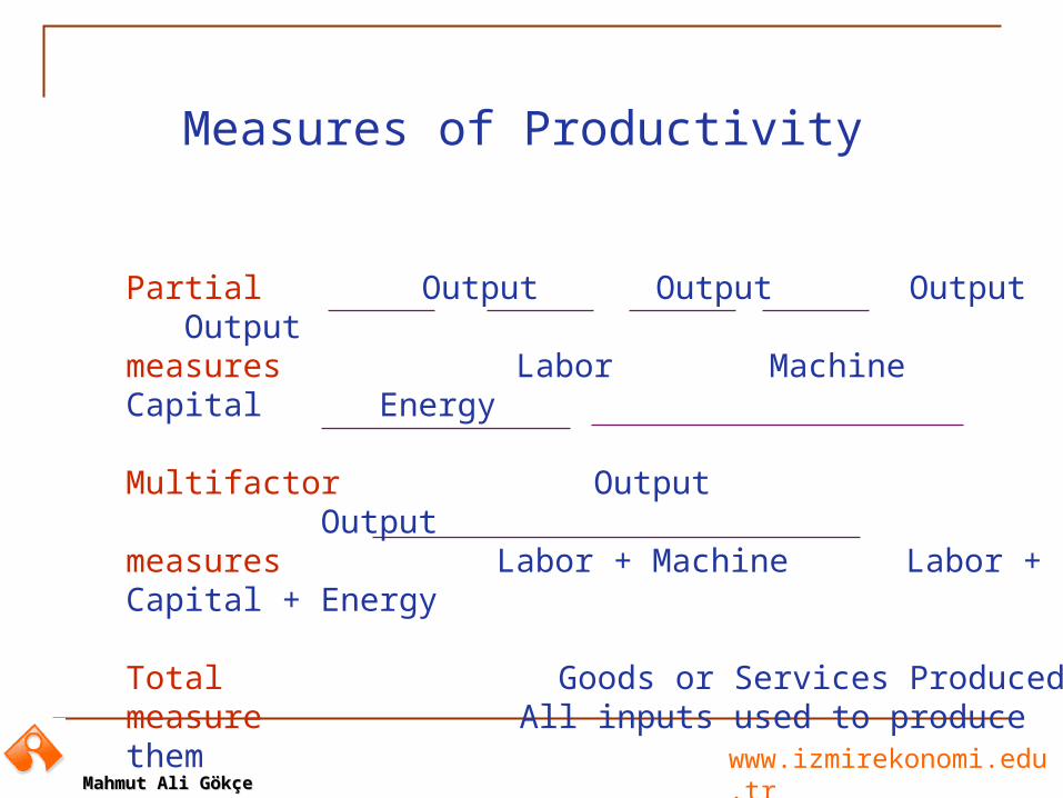
Measures of Productivity
Partial Output Output Output Outputmeasures Labor Machine Capital Energy
Multifactor Output Outputmeasures Labor + Machine Labor + Capital + Energy
Total Goods or Services Producedmeasure All inputs used to produce them
www.izmirekonomi.edu.trMahmut Ali GökçeMahmut Ali Gökçe
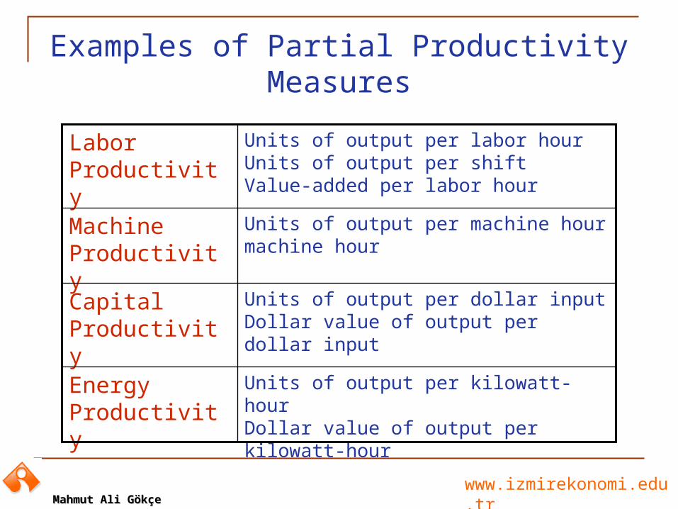
Units of output per kilowatt-hourDollar value of output per kilowatt-hour
Energy Productivity
Units of output per dollar inputDollar value of output per dollar input
Capital Productivity
Units of output per machine hourmachine hour
Machine Productivity
Units of output per labor hourUnits of output per shiftValue-added per labor hour
Labor Productivity
Examples of Partial Productivity Measures

www.izmirekonomi.edu.trMahmut Ali GökçeMahmut Ali Gökçe
How to use “Productivity”? Productivity measures can be used to track
performance over time. This allows managers to judge performance and and to decide where improvements are needed. If productivity has slipped in a certain area
examine the factors and determine the reasons
Productivity also can be used to benchmark the companies standing with respect to competitors. How to position the company with respect to the
“best in the classroom”. Determine the areas the company is behind and take actions accordingly.

www.izmirekonomi.edu.trMahmut Ali GökçeMahmut Ali Gökçe
Example: Productivity10,000 Units Produced
Sold for $10/unit
500 labor hours
Labor rate: $9/hr
Cost of raw material: $5,000
Cost of purchased material: $25,000
What is the labor productivity?
www.izmirekonomi.edu.trMahmut Ali GökçeMahmut Ali Gökçe
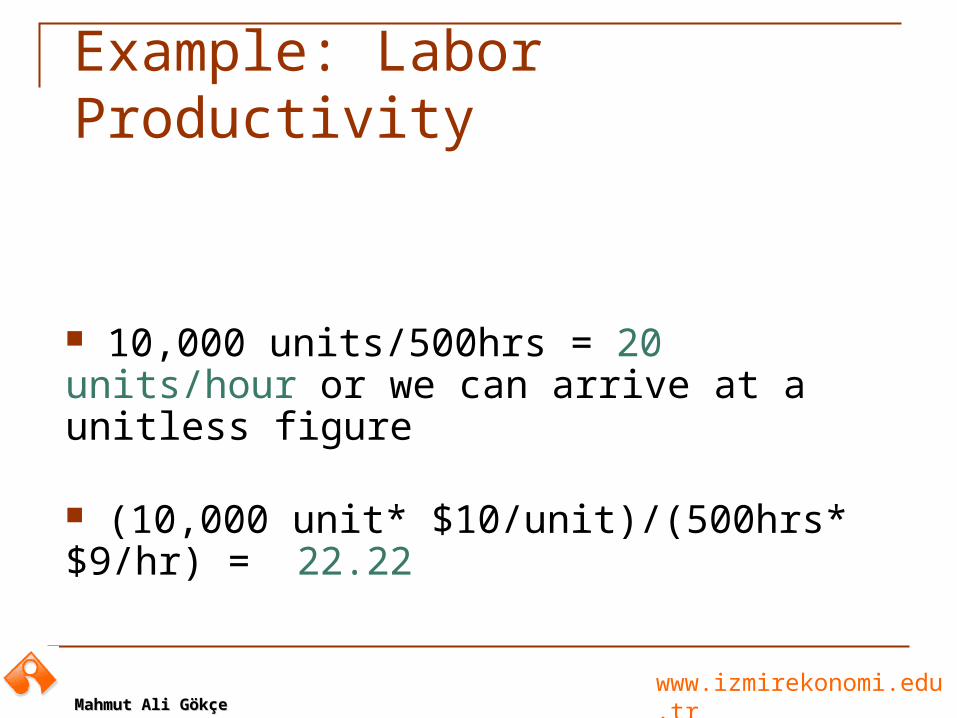
10,000 units/500hrs = 20 units/hour or we can arrive at a unitless figure
(10,000 unit* $10/unit)/(500hrs* $9/hr) = 22.22
Example: Labor Productivity
www.izmirekonomi.edu.trMahmut Ali GökçeMahmut Ali Gökçe
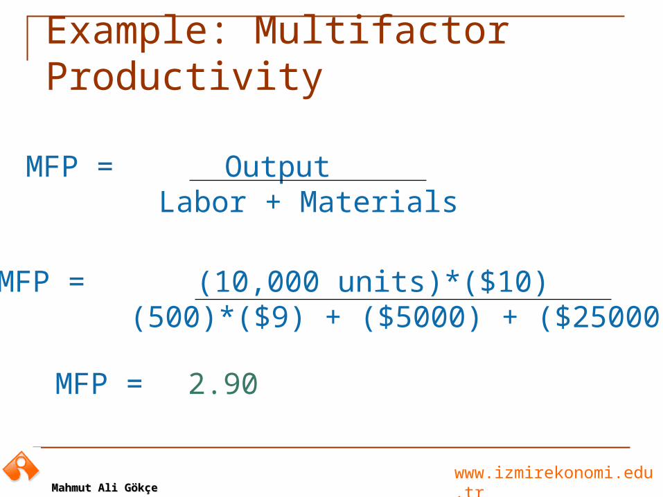
Example: Multifactor Productivity
MFP = OutputLabor + Materials
MFP = (10,000 units)*($10)(500)*($9) + ($5000) + ($25000)
MFP = 2.90

www.izmirekonomi.edu.trMahmut Ali GökçeMahmut Ali Gökçe
From Idea to ProductDecision problems
Forecasting Product and service design Capacity Planning Facilities Layout Location Transportation/assignment Inventory Aggregate Planning Scheduling Project Management
www.izmirekonomi.edu.trMahmut Ali GökçeMahmut Ali Gökçe
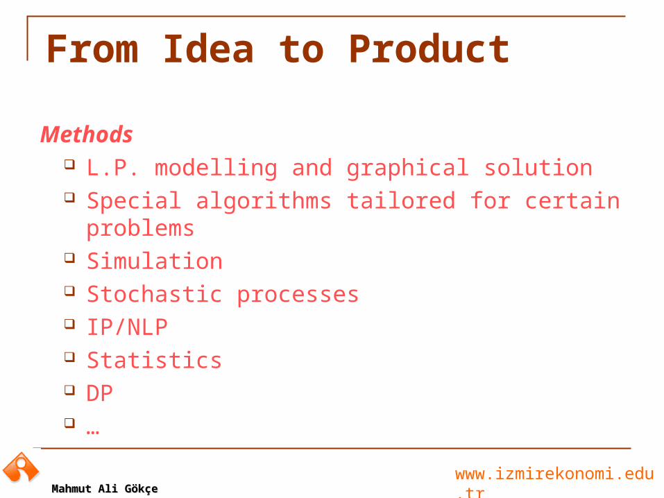
From Idea to Product
Methods L.P. modelling and graphical solution Special algorithms tailored for certain problems Simulation Stochastic processes IP/NLP Statistics DP …
www.izmirekonomi.edu.trMahmut Ali GökçeMahmut Ali Gökçe
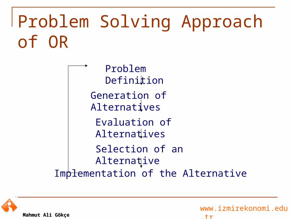
Problem Solving Approach of OR
Problem Definition
Generation of Alternatives
Evaluation of Alternatives
Selection of an Alternative
Implementation of the Alternative
www.izmirekonomi.edu.trMahmut Ali GökçeMahmut Ali Gökçe
What Is A Model ?
A model is the selected abstract representation of a real situation or behaviour with suitable language or expression.
Since a model is an explicit representation of reality, it is generally less complex than reality.
The level of abstraction depends on the subject, the purpose, and the environment of modelling.
It is important that it is sufficiently complete to approximate those aspects of reality to be investigated.
www.izmirekonomi.edu.trMahmut Ali GökçeMahmut Ali Gökçe
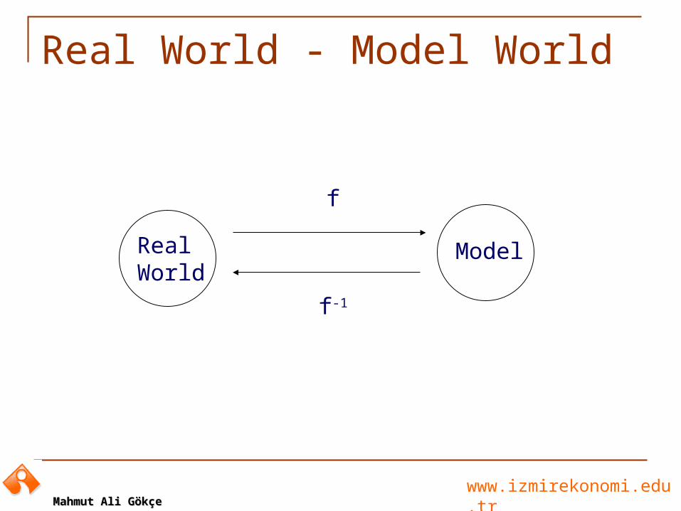
Real World - Model World
RealWorld
Model
f
f-1
www.izmirekonomi.edu.trMahmut Ali GökçeMahmut Ali Gökçe
Types of Models
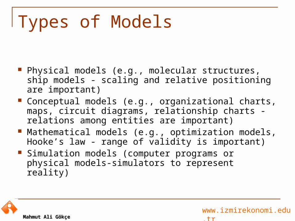
Physical models (e.g., molecular structures, ship models - scaling and relative positioning are important)
Conceptual models (e.g., organizational charts, maps, circuit diagrams, relationship charts - relations among entities are important)
Mathematical models (e.g., optimization models, Hooke’s law - range of validity is important)
Simulation models (computer programs or physical models-simulators to represent reality)
www.izmirekonomi.edu.trMahmut Ali GökçeMahmut Ali Gökçe
Purposes of Modelling
To understand better the subject of modelling.
To describe the subject of modelling.
To create a means to exchange views on the subject.
To predict and control the behaviour of the subject.
www.izmirekonomi.edu.trMahmut Ali GökçeMahmut Ali Gökçe
Advantages of modeling a Business System Definition of business objectives, practices,
structure, and constraints Definition and establishment of business
parameters and costs Systematic evaluation of alternative system
alternatives Quick response through sensitivity analysis
www.izmirekonomi.edu.trMahmut Ali GökçeMahmut Ali Gökçe
Tradeoffs in Modeling
Realism vs. Solvability Decision Support vs. Decision Making
www.izmirekonomi.edu.trMahmut Ali GökçeMahmut Ali Gökçe
Operations Research :Model Types Descriptive Models (Decision support)
Statistics Simulation Queuing …
Prescriptive Models (Decision making) Optimization
Linear Programming Nonlinear Programming Network Flows
…
www.izmirekonomi.edu.trMahmut Ali GökçeMahmut Ali Gökçe
Algorithms to Solve Models
An algorithm is a recipe to solve a problem. “A step-by-step problem-solving procedure,
especially an established, recursive computational procedure for solving a problem in a finite number of steps.” ( http://www.dictionary.com ) Efficient vs. Effective Optimal vs. Heuristic Primal vs. Dual Construction vs. Improvement Alternative Generating vs. Alternative Selecting

27www.izmirekonomi.edu.trMahmut Mahmut Ali GökçeAli Gökçe
FORECASTING
www.izmirekonomi.edu.trMahmut Ali GökçeMahmut Ali Gökçe
Introduction
Forecasting is to predict the future by analysis of relevant data.
Forecasts are the basis (input) for a wide range of decisions in operations management and control.
Forecasts are typically developed by the ‘Marketing’ function, but ‘Operations’ function is usually called on to assist in its development.
Furthermore, ‘Operations’ is the major user of forecasts.
One can forecast anything. We will focus on demand forecast. But techniques are there!
www.izmirekonomi.edu.trMahmut Ali GökçeMahmut Ali Gökçe
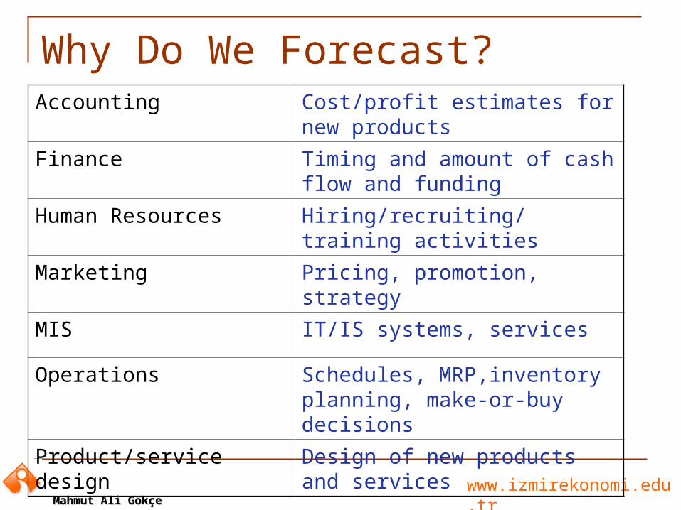
Why Do We Forecast?Accounting Cost/profit estimates for new
products
Finance Timing and amount of cash flow and funding
Human Resources Hiring/recruiting/training activities
Marketing Pricing, promotion, strategy
MIS IT/IS systems, services
Operations Schedules, MRP,inventory planning, make-or-buy decisions
Product/service design Design of new products and services
www.izmirekonomi.edu.trMahmut Ali GökçeMahmut Ali Gökçe
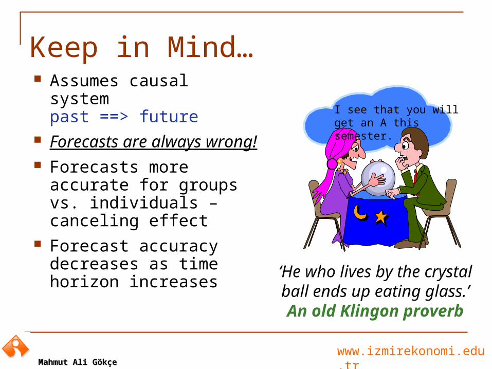
Assumes causal systempast ==> future
Forecasts are always wrong!
Forecasts more accurate for groups vs. individuals – canceling effect
Forecast accuracy decreases as time horizon increases
I see that you willget an A this semester.
Keep in Mind…
‘He who lives by the crystal ball ends up eating glass.’
An old Klingon proverb
www.izmirekonomi.edu.trMahmut Ali GökçeMahmut Ali Gökçe
Types of Forecasts
Judgmental - uses subjective input such as market surveys, expert opinion, etc.
Time series - uses historical data assuming the future will be like the past
Associative models (casual models) - uses explanatory variables to predict the future, demand for paint might be related to variables such as price, quality, etc.
www.izmirekonomi.edu.trMahmut Ali GökçeMahmut Ali Gökçe
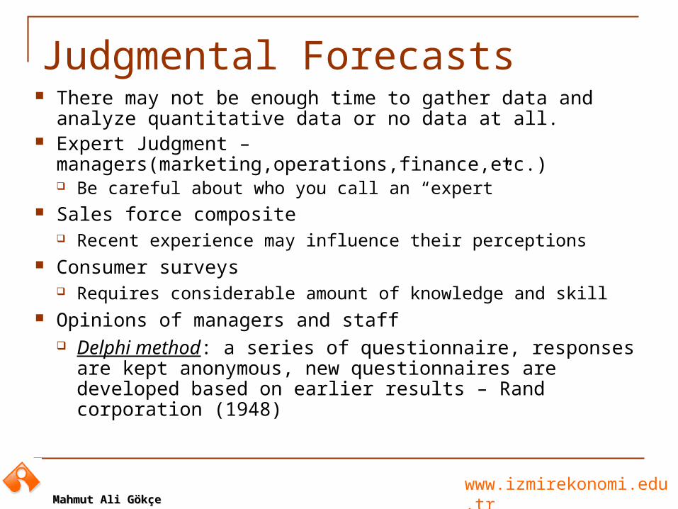
Judgmental Forecasts There may not be enough time to gather data and analyze
quantitative data or no data at all. Expert Judgment – managers(marketing,operations,finance,etc.)
Be careful about who you call an “expert” Sales force composite
Recent experience may influence their perceptions Consumer surveys
Requires considerable amount of knowledge and skill Opinions of managers and staff
Delphi method: a series of questionnaire, responses are kept anonymous, new questionnaires are developed based on earlier results – Rand corporation (1948)
www.izmirekonomi.edu.trMahmut Ali GökçeMahmut Ali Gökçe
Time Series Model Building
A time-series is a time ordered sequence of observations taken at regular intervals over a period of time.
The data may be demand, earnings, profit, accidents, consumer price index,etc.
The assumption is future values of the series can be estimated from past values
One need to identify the underlying behavior of the series - pattern of the data
www.izmirekonomi.edu.trMahmut Ali GökçeMahmut Ali Gökçe
Some Behaviors Typically Observed
Trend E.g., population shifts, change in income. Usually a long-term
movement in data Seasonality
Fairly regular variations, e.g., Friday nights in restaurants, new year in shopping malls, rush hour traffic., etc.
Cycles Wavelike variations lasting more than a year, e.g. economic recessions,
etc. Irregular variations
Caused by unusual circumstances, e.g., strikes, weather conditions, etc.
Random variations Residual variations after all other behaviors are accounted for.
Caused by chance
www.izmirekonomi.edu.trMahmut Ali GökçeMahmut Ali Gökçe
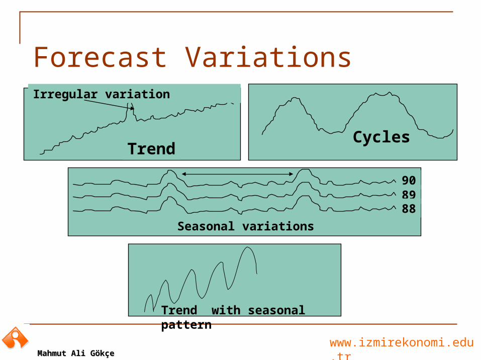
Forecast Variations
Trend
Irregular variation
Seasonal variations
908988
Cycles
Trend with seasonal pattern
www.izmirekonomi.edu.trMahmut Ali GökçeMahmut Ali Gökçe
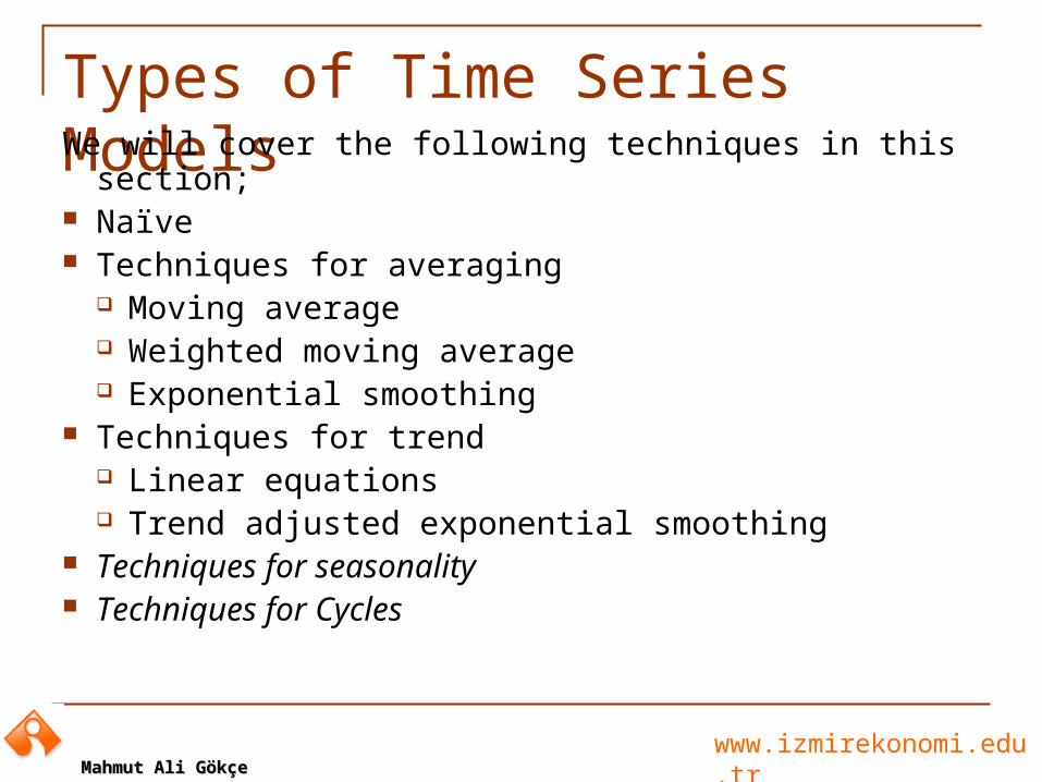
Types of Time Series ModelsWe will cover the following techniques in this section; Naïve Techniques for averaging
Moving average Weighted moving average Exponential smoothing
Techniques for trend Linear equations Trend adjusted exponential smoothing
Techniques for seasonality Techniques for Cycles

www.izmirekonomi.edu.trMahmut Ali GökçeMahmut Ali Gökçe
Naive Forecasts
Uh, give me a minute.... We sold 250 wheels lastweek.... Now, next week we should sell....
www.izmirekonomi.edu.trMahmut Ali GökçeMahmut Ali Gökçe
Simple and widely used technique. A single previous value of a time series as the basis
for forecast. Virtually no cost. Data analysis is nonexistent, easily understandable Cannot provide high accuracy, may be used as a
standard for accuracy. Can be used in case of,
Stable series Series with seasonality Series with trend
Naïve Forecasts
www.izmirekonomi.edu.trMahmut Ali GökçeMahmut Ali Gökçe
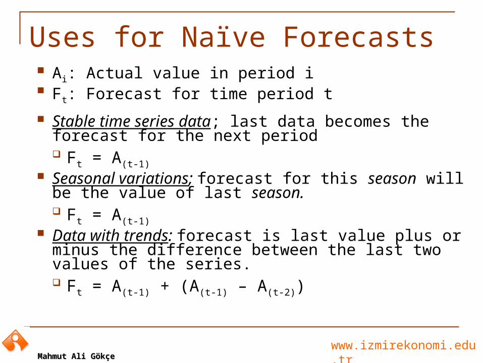
Ai: Actual value in period i Ft: Forecast for time period t
Stable time series data; last data becomes the forecast for the next period Ft = A(t-1)
Seasonal variations; forecast for this season will be the value of last season. Ft = A(t-1)
Data with trends: forecast is last value plus or minus the difference between the last two values of the series. Ft = A(t-1) + (A(t-1) – A(t-2))
Uses for Naïve Forecasts
www.izmirekonomi.edu.trMahmut Ali GökçeMahmut Ali Gökçe
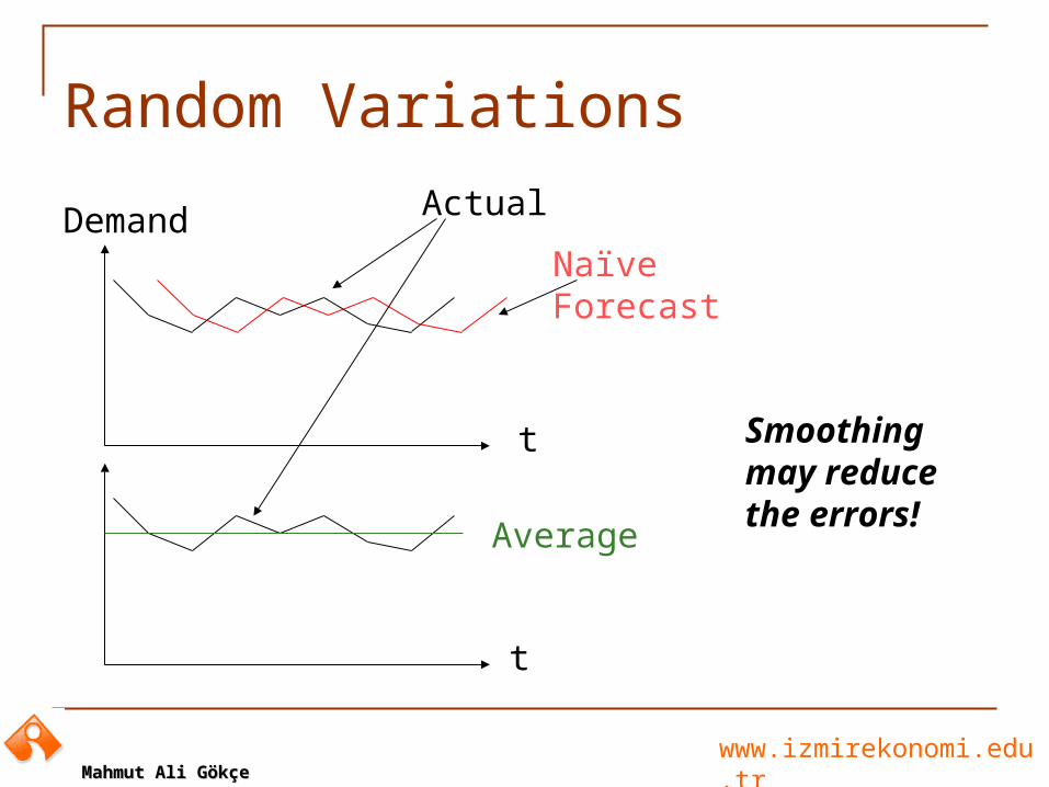
Random Variations
Demand
t
Actual
Naïve Forecast
t
Average
Smoothing may reduce the errors!
www.izmirekonomi.edu.trMahmut Ali GökçeMahmut Ali Gökçe
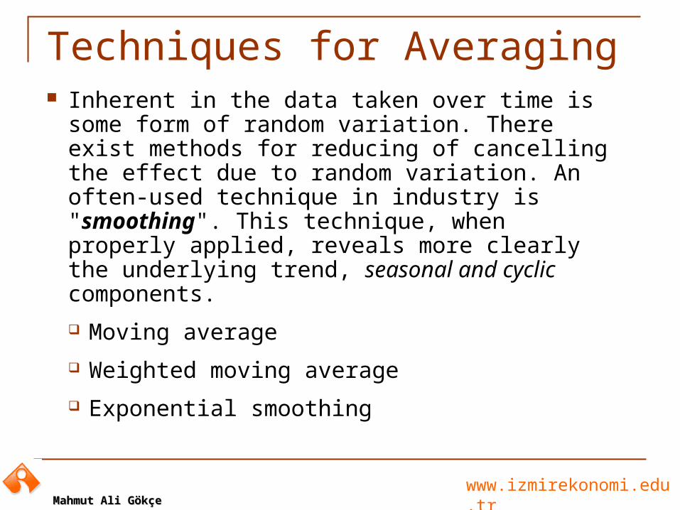
Techniques for Averaging Inherent in the data taken over time is some form
of random variation. There exist methods for reducing of cancelling the effect due to random variation. An often-used technique in industry is "smoothing". This technique, when properly applied, reveals more clearly the underlying trend, seasonal and cyclic components.
Moving average
Weighted moving average
Exponential smoothing
www.izmirekonomi.edu.trMahmut Ali GökçeMahmut Ali Gökçe
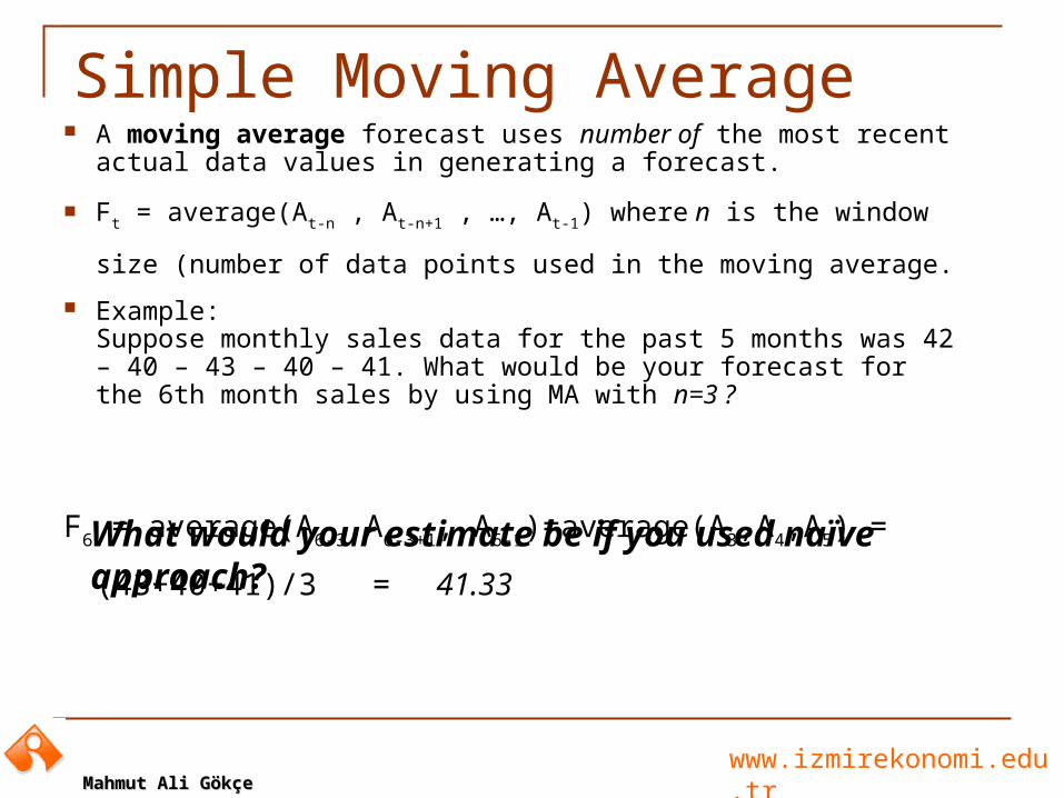
Simple Moving Average A moving average forecast uses number of the most recent
actual data values in generating a forecast.
Ft = average(At-n , At-n+1 , …, At-1) where n is the window size
(number of data points used in the moving average.
Example:Suppose monthly sales data for the past 5 months was 42 – 40 – 43 – 40 – 41. What would be your forecast for the 6th month sales by using MA with n=3 ?
F6 = average(A6-3,A6-3+1, A6-1)=average(A3,A4,A5) =
(43+40+41)/3 = 41.33
What would your estimate be if you used naïve approach?
www.izmirekonomi.edu.trMahmut Ali GökçeMahmut Ali Gökçe
Simple Moving Average - Example
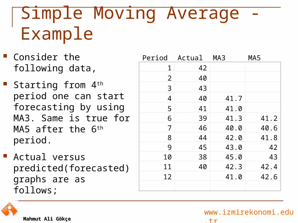
Period Actual MA3 MA5
1 42
2 40
3 43
4 40 41.7
5 41 41.0 6 39 41.3 41.27 46 40.0 40.68 44 42.0 41.89 45 43.0 42
10 38 45.0 4311 40 42.3 42.4
12 41.0 42.6
Consider the following data,
Starting from 4th period one can start forecasting by using MA3. Same is true for MA5 after the 6th period.
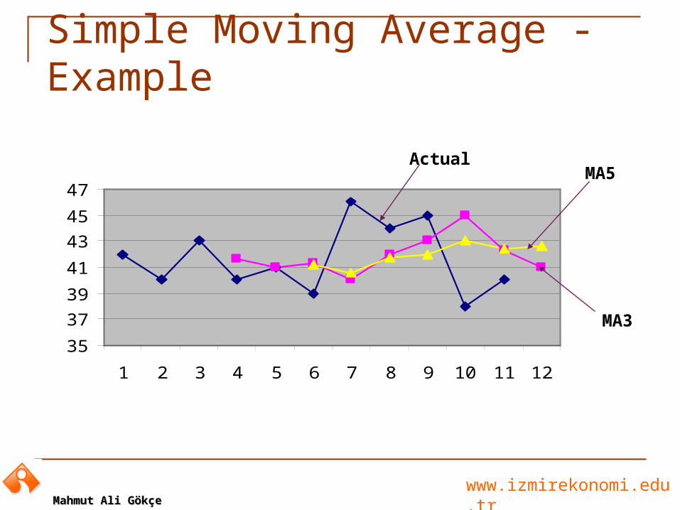
Actual versus predicted(forecasted) graphs are as follows;
www.izmirekonomi.edu.trMahmut Ali GökçeMahmut Ali Gökçe
Simple Moving Average - Example
35
37
39
41
43
45
47
1 2 3 4 5 6 7 8 9 10 11 12
Actual
MA3
MA5
www.izmirekonomi.edu.trMahmut Ali GökçeMahmut Ali Gökçe
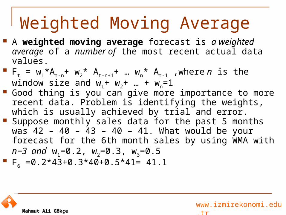
Weighted Moving Average A weighted moving average forecast is a weighted
average of a number of the most recent actual data values. Ft = w1*At-n+ w2* At-n+1+ … wn* At-1 ,where n is the window
size and w1+ w2+ … + wn=1 Good thing is you can give more importance to more recent
data. Problem is identifying the weights, which is usually achieved by trial and error.
Suppose monthly sales data for the past 5 months was 42 – 40 – 43 – 40 – 41. What would be your forecast for the 6th month sales by using WMA with n=3 and w1=0.2, w2=0.3, w3=0.5
F6 =0.2*43+0.3*40+0.5*41= 41.1
www.izmirekonomi.edu.trMahmut Ali GökçeMahmut Ali Gökçe
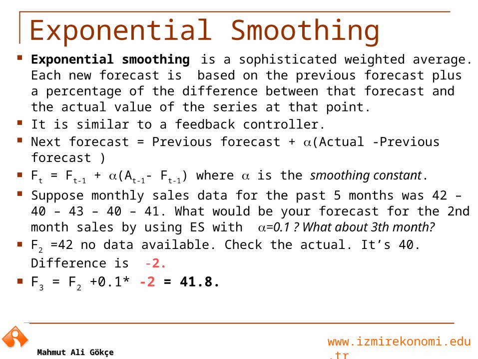
Exponential Smoothing Exponential smoothing is a sophisticated weighted average.
Each new forecast is based on the previous forecast plus a percentage of the difference between that forecast and the actual value of the series at that point.
It is similar to a feedback controller. Next forecast = Previous forecast + (Actual -Previous forecast ) Ft = Ft-1 + (At-1- Ft-1) where is the smoothing constant. Suppose monthly sales data for the past 5 months was 42 – 40 –
43 – 40 – 41. What would be your forecast for the 2nd month sales by using ES with =0.1 ? What about 3th month?
F2 =42 no data available. Check the actual. It’s 40. Difference is
-2. F3 = F2 +0.1* -2 = 41.8.
www.izmirekonomi.edu.trMahmut Ali GökçeMahmut Ali Gökçe
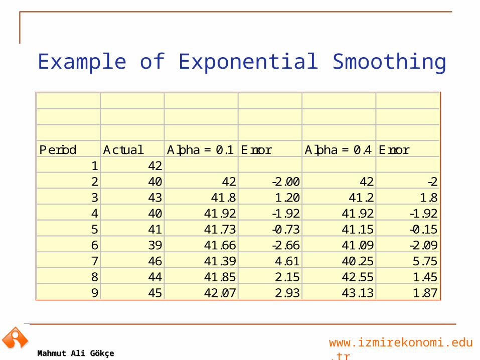
Period Actual Alpha = 0.1 Error Alpha = 0.4 Error1 422 40 42 -2.00 42 -23 43 41.8 1.20 41.2 1.84 40 41.92 -1.92 41.92 -1.925 41 41.73 -0.73 41.15 -0.156 39 41.66 -2.66 41.09 -2.097 46 41.39 4.61 40.25 5.758 44 41.85 2.15 42.55 1.459 45 42.07 2.93 43.13 1.87
Example of Exponential Smoothing
www.izmirekonomi.edu.trMahmut Ali GökçeMahmut Ali Gökçe
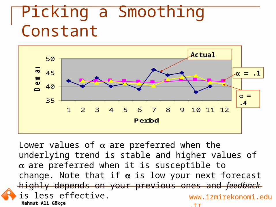
Picking a Smoothing Constant
35
40
45
50
1 2 3 4 5 6 7 8 9 10 11 12
Period
De
ma
nd
.1
.4
Actual
Lower values of are preferred when the underlying trend is stable and higher values of are preferred when it is susceptible to change. Note that if is low your next forecast highly depends on your previous ones and feedback is less effective.
www.izmirekonomi.edu.trMahmut Ali GökçeMahmut Ali Gökçe
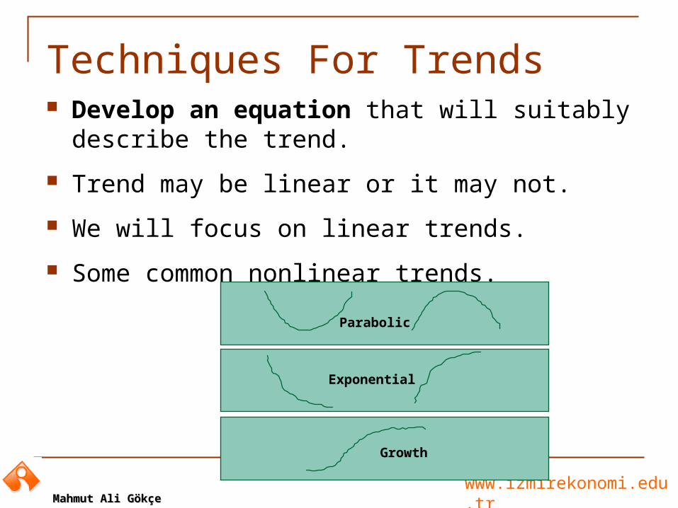
Techniques For Trends Develop an equation that will suitably describe the
trend.
Trend may be linear or it may not.
We will focus on linear trends.
Some common nonlinear trends.
Parabolic
Exponential
Growth
www.izmirekonomi.edu.trMahmut Ali GökçeMahmut Ali Gökçe
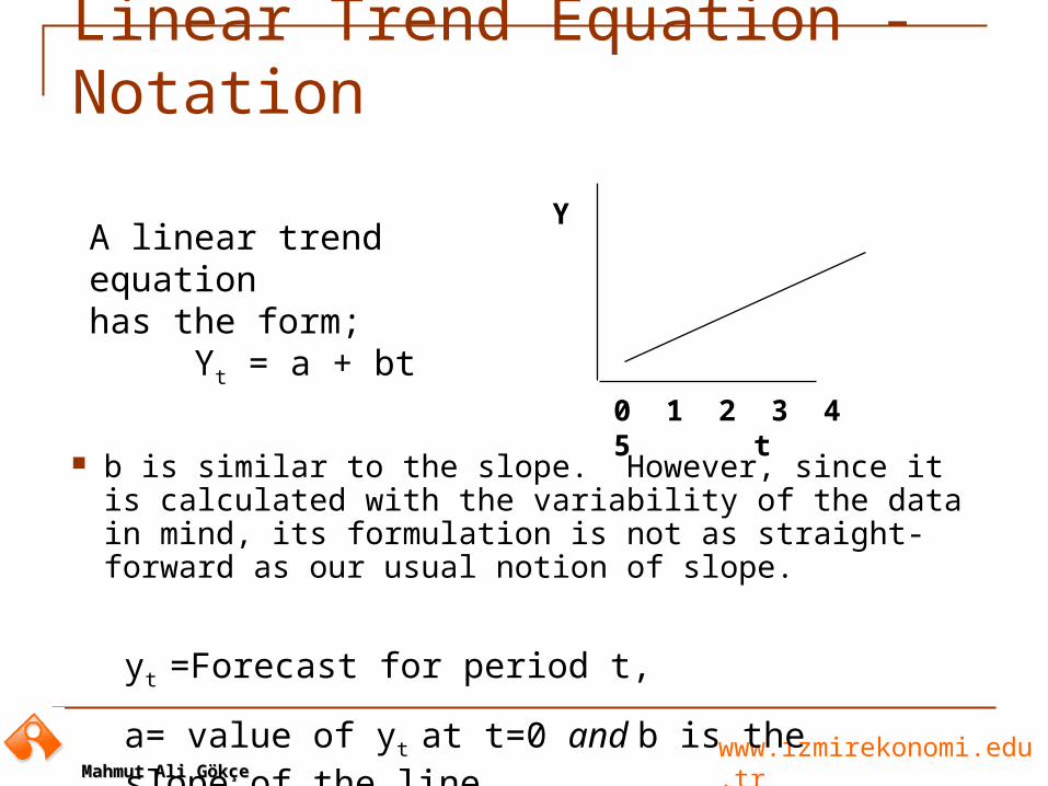
Linear Trend Equation - Notation
b is similar to the slope. However, since it is calculated with the variability of the data in mind, its formulation is not as straight-forward as our usual notion of slope.
A linear trend equation has the form;
Yt = a + bt
0 1 2 3 4 5 t
Y
yt =Forecast for period t,
a= value of yt at t=0 and b is the slope of the line.
www.izmirekonomi.edu.trMahmut Ali GökçeMahmut Ali Gökçe
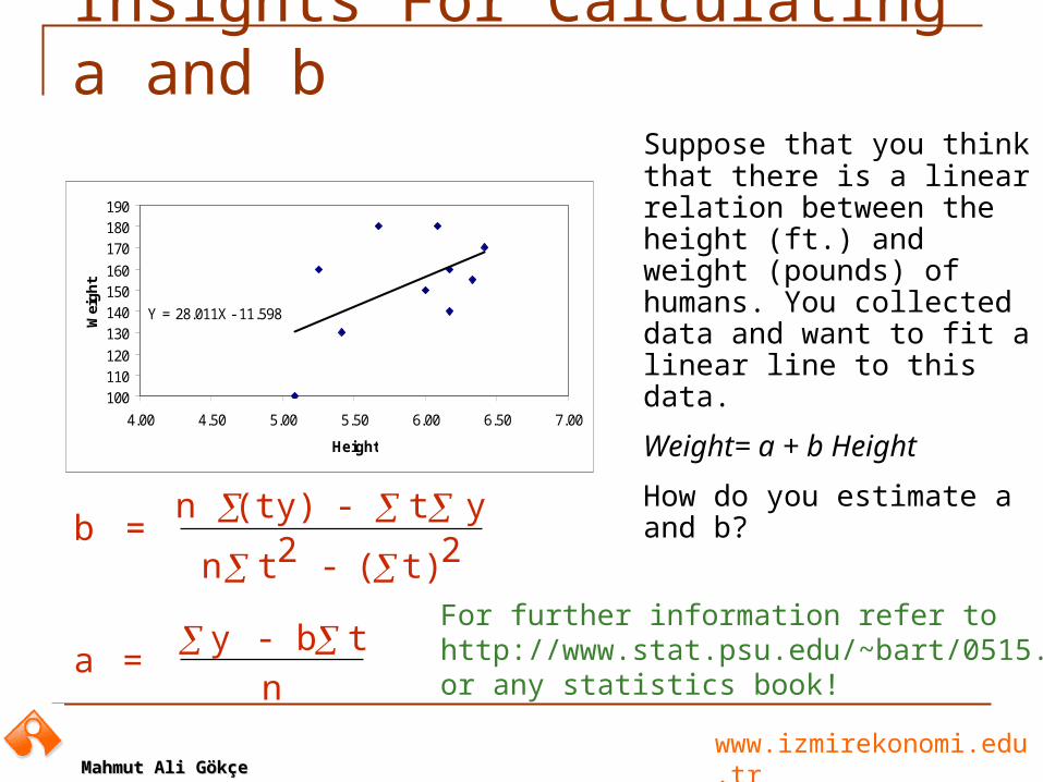
Insights For Calculating a and b
b = n (ty) - t y
n t 2 - ( t) 2
a = y - b t
n
Y = 28.011X - 11.598
100110120
130140150160
170180190
4.00 4.50 5.00 5.50 6.00 6.50 7.00
Height
Wei
gh
t
For further information refer tohttp://www.stat.psu.edu/~bart/0515.docor any statistics book!
Suppose that you think that there is a linear relation between the height (ft.) and weight (pounds) of humans. You collected data and want to fit a linear line to this data.
Weight= a + b Height
How do you estimate a and b?
www.izmirekonomi.edu.trMahmut Ali GökçeMahmut Ali Gökçe
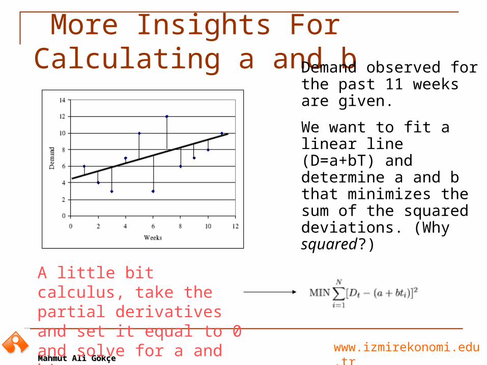
More Insights For Calculating a and bDemand observed for
the past 11 weeks are given.
We want to fit a linear line (D=a+bT) and determine a and b that minimizes the sum of the squared deviations. (Why squared?)
A little bit calculus, take the partial derivatives and set it equal to 0 and solve for a and b!
www.izmirekonomi.edu.trMahmut Ali GökçeMahmut Ali Gökçe
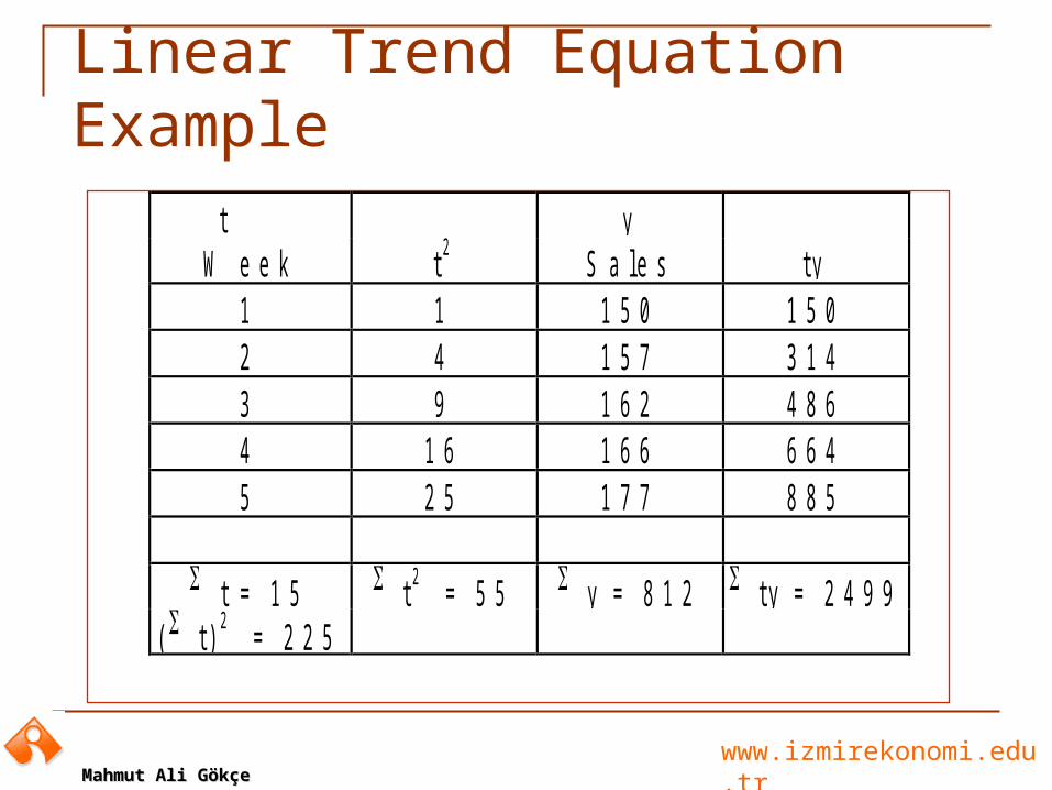
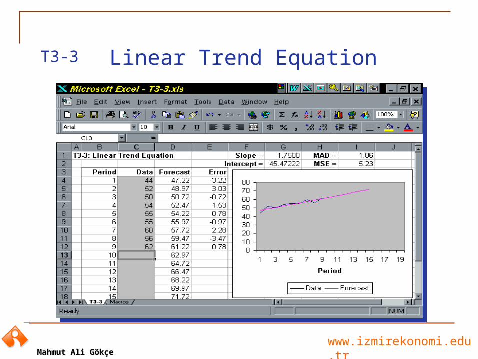
Linear Trend Equation Example
t yW e e k t 2 S a l e s t y
1 1 1 5 0 1 5 02 4 1 5 7 3 1 43 9 1 6 2 4 8 64 1 6 1 6 6 6 6 45 2 5 1 7 7 8 8 5
t = 1 5 t 2 = 5 5 y = 8 1 2 t y = 2 4 9 9( t ) 2 = 2 2 5
www.izmirekonomi.edu.trMahmut Ali GökçeMahmut Ali Gökçe
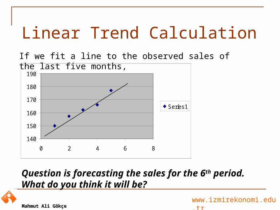
Linear Trend Calculation
140
150
160
170
180
190
0 2 4 6 8
Series1
Question is forecasting the sales for the 6th period. What do you think it will be?
If we fit a line to the observed sales of the last five months,
www.izmirekonomi.edu.trMahmut Ali GökçeMahmut Ali Gökçe
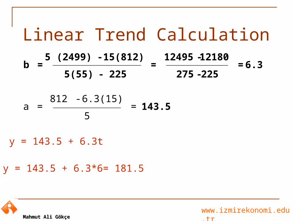
Linear Trend Calculation
y = 143.5 + 6.3t
a = 812 - 6.3(15)
5 =
b = 5 (2499) - 15(812)
5(55) - 225 =
12495 -12180
275 -225 = 6.3
143.5
y = 143.5 + 6.3*6= 181.5
www.izmirekonomi.edu.trMahmut Ali GökçeMahmut Ali Gökçe
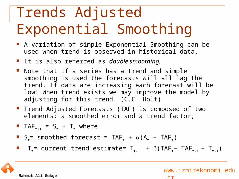
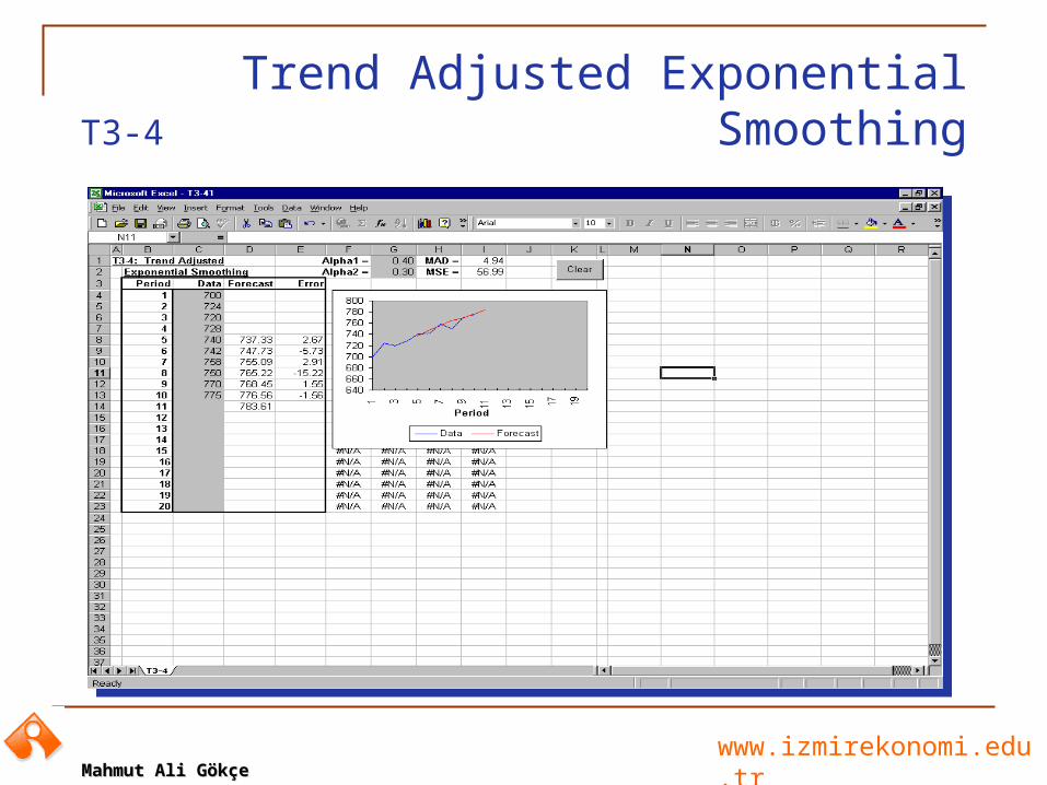
Trends Adjusted Exponential Smoothing A variation of simple Exponential Smoothing can be used
when trend is observed in historical data. It is also referred as double smoothing. Note that if a series has a trend and simple smoothing is used
the forecasts will all lag the trend. If data are increasing each forecast will be low! When trend exists we may improve the model by adjusting for this trend. (C.C. Holt)
Trend Adjusted Forecasts (TAF) is composed of two elements: a smoothed error and a trend factor;
TAFt+1 = St + Tt where
St= smoothed forecast = TAFt + (At – TAFt)
Tt= current trend estimate= Tt-1 + (TAFt– TAFt-1 – Tt-1)
www.izmirekonomi.edu.trMahmut Ali GökçeMahmut Ali Gökçe
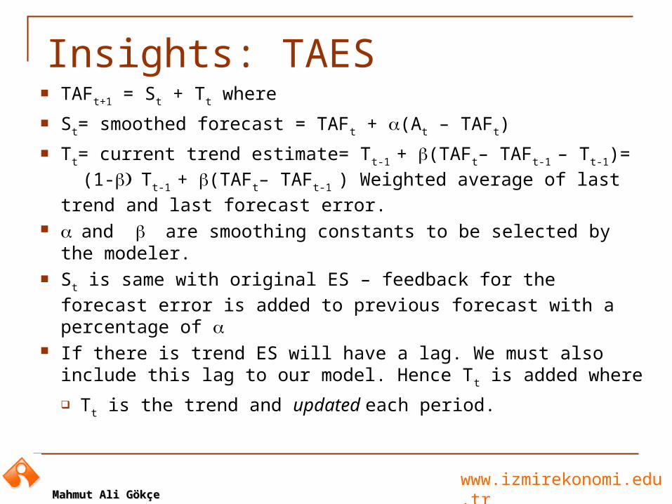
Insights: TAES TAFt+1 = St + Tt where
St= smoothed forecast = TAFt + (At – TAFt)
Tt= current trend estimate= Tt-1 + (TAFt– TAFt-1 – Tt-1)= (1-
Tt-1 + (TAFt– TAFt-1 ) Weighted average of last trend and
last forecast error. and are smoothing constants to be selected by the
modeler. St is same with original ES – feedback for the forecast error
is added to previous forecast with a percentage of If there is trend ES will have a lag. We must also include this
lag to our model. Hence Tt is added where
Tt is the trend and updated each period.
www.izmirekonomi.edu.trMahmut Ali GökçeMahmut Ali Gökçe
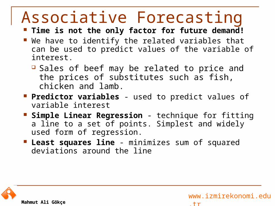
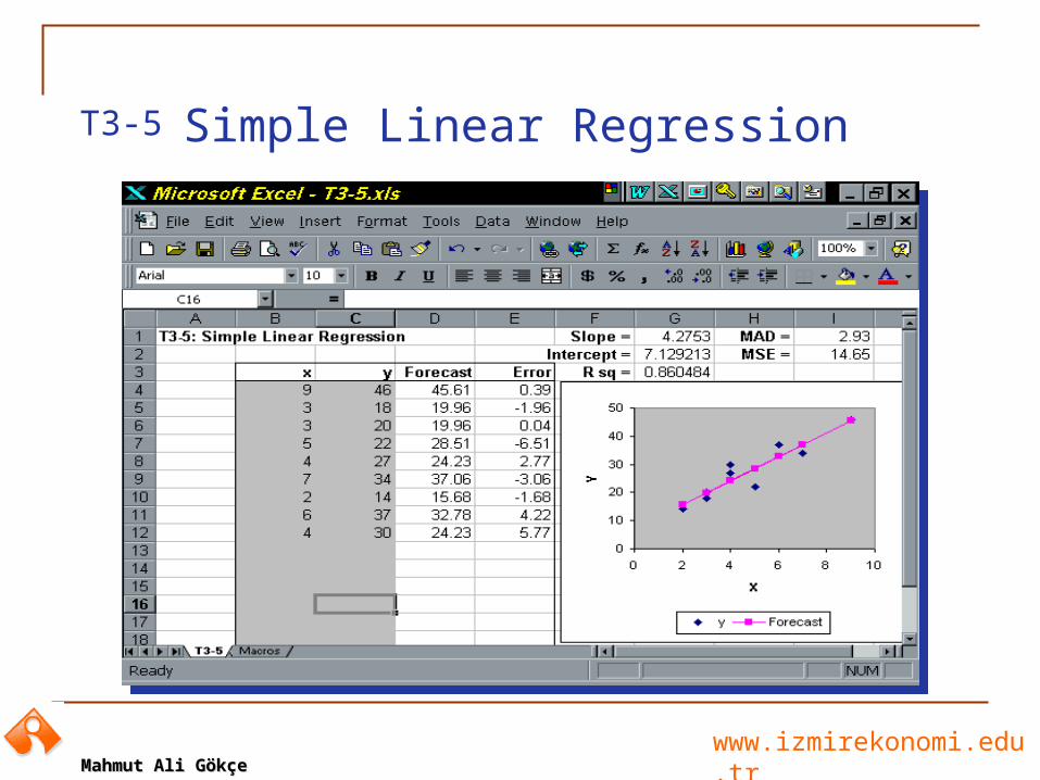
Associative Forecasting Time is not the only factor for future demand! We have to identify the related variables that can be used
to predict values of the variable of interest. Sales of beef may be related to price and the prices
of substitutes such as fish, chicken and lamb. Predictor variables - used to predict values of variable
interest Simple Linear Regression - technique for fitting a line to
a set of points. Simplest and widely used form of regression.
Least squares line - minimizes sum of squared deviations around the line
www.izmirekonomi.edu.trMahmut Ali GökçeMahmut Ali Gökçe
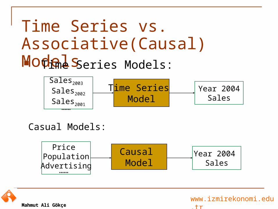
Time Series vs. Associative(Causal) Models Time Series Models:
Causal Model
Year 2004 Sales
Price PopulationAdvertising
……
Casual Models:
Time Series Model
Year 2004Sales
Sales2003 Sales2002
Sales2001……
www.izmirekonomi.edu.trMahmut Ali GökçeMahmut Ali Gökçe
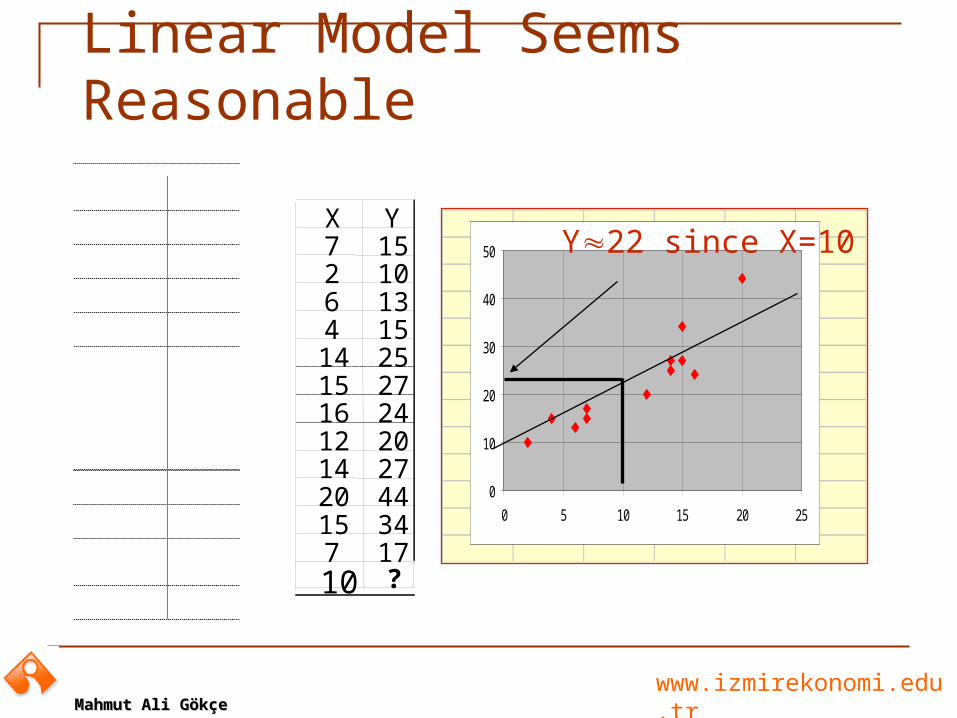
Linear Model Seems Reasonable
0
10
20
30
40
50
0 5 10 15 20 25
X Y7 152 106 134 1514 2515 2716 2412 2014 2720 4415 347 17
Y22 since X=10
10 ?
www.izmirekonomi.edu.trMahmut Ali GökçeMahmut Ali Gökçe
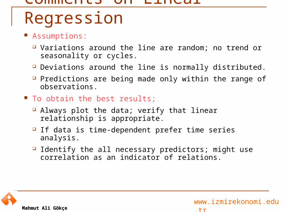
Comments on Linear Regression Assumptions:
Variations around the line are random; no trend or seasonality or cycles.
Deviations around the line is normally distributed. Predictions are being made only within the range of
observations.
To obtain the best results; Always plot the data; verify that linear relationship is
appropriate. If data is time-dependent prefer time series analysis. Identify the all necessary predictors; might use correlation as
an indicator of relations.
www.izmirekonomi.edu.trMahmut Ali GökçeMahmut Ali Gökçe
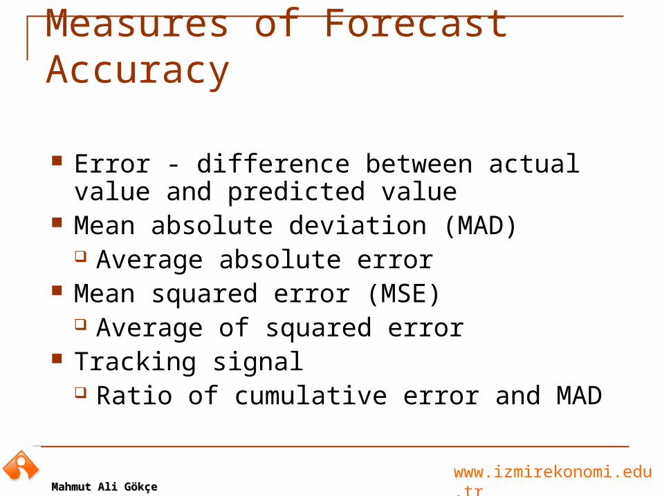
Measures of Forecast Accuracy
Error - difference between actual value and predicted value
Mean absolute deviation (MAD) Average absolute error
Mean squared error (MSE) Average of squared error
Tracking signal Ratio of cumulative error and MAD
www.izmirekonomi.edu.trMahmut Ali GökçeMahmut Ali Gökçe
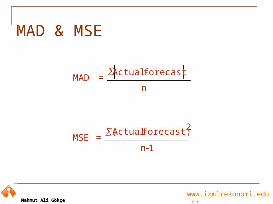
MAD & MSE
MAD = Actual forecast
n
MSE = Actual forecast)
-1
2
n
(
www.izmirekonomi.edu.trMahmut Ali GökçeMahmut Ali Gökçe
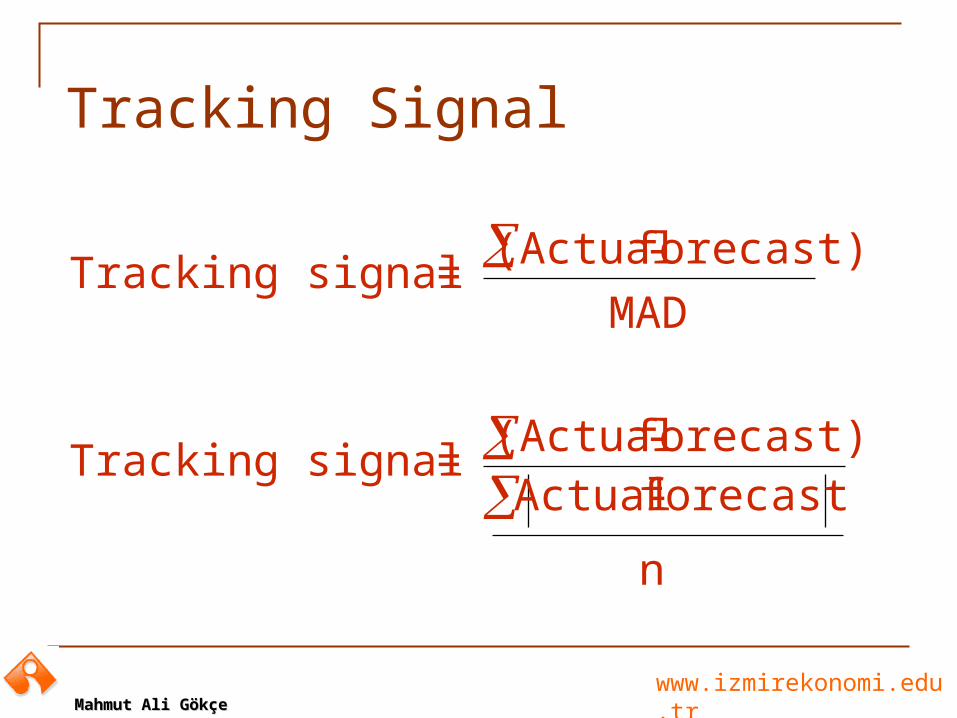
Tracking Signal
Tracking signal = (Actual-forecast)
MAD
Tracking signal = (Actual-forecast)Actual-forecast
n
www.izmirekonomi.edu.trMahmut Ali GökçeMahmut Ali Gökçe
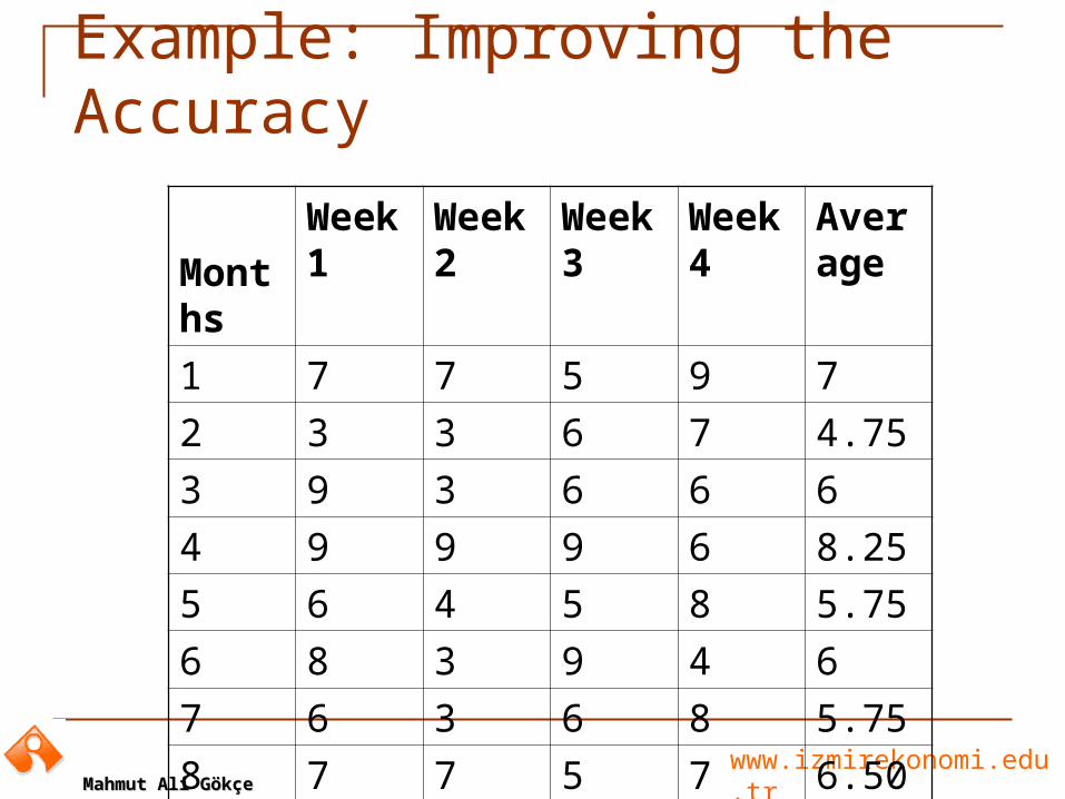
Example: Improving the Accuracy
Months
Week 1
Week 2
Week 3
Week 4
Average
1 7 7 5 9 7
2 3 3 6 7 4.75
3 9 3 6 6 6
4 9 9 9 6 8.25
5 6 4 5 8 5.75
6 8 3 9 4 6
7 6 3 6 8 5.75
8 7 7 5 7 6.50
www.izmirekonomi.edu.trMahmut Ali GökçeMahmut Ali Gökçe
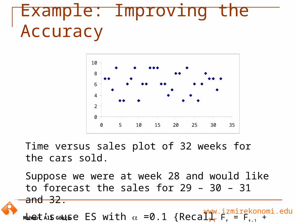
Example: Improving the Accuracy
Time versus sales plot of 32 weeks for the cars sold.
Suppose we were at week 28 and would like to forecast the sales for 29 – 30 – 31 and 32.
Let’s use ES with =0.1 {Recall Ft = Ft-1 + (At-1- Ft-1) }
0
2
4
6
8
10
0 5 10 15 20 25 30 35
www.izmirekonomi.edu.trMahmut Ali GökçeMahmut Ali Gökçe
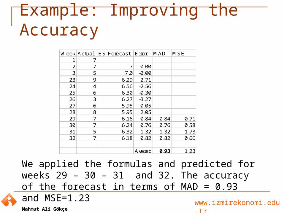
Example: Improving the Accuracy
We applied the formulas and predicted for weeks 29 – 30 – 31 and 32. The accuracy of the forecast in terms of MAD = 0.93 and MSE=1.23
Week Actual ES Forecast Error MAD MSE1 72 7 7 0.003 5 7.0 -2.004 9 6.80 2.20
23 9 6.29 2.7124 4 6.56 -2.5625 6 6.30 -0.3026 3 6.27 -3.2727 6 5.95 0.0528 8 5.95 2.0529 7 6.16 0.84 0.84 0.7130 7 6.24 0.76 0.76 0.5831 5 6.32 -1.32 1.32 1.7332 7 6.18 0.82 0.82 0.66
Average= 0.93 1.23
www.izmirekonomi.edu.trMahmut Ali GökçeMahmut Ali Gökçe
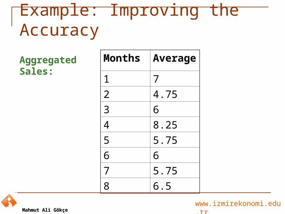
Example: Improving the Accuracy
Months Average
1 7
2 4.75
3 6
4 8.25
5 5.75
6 6
7 5.75
8 6.5
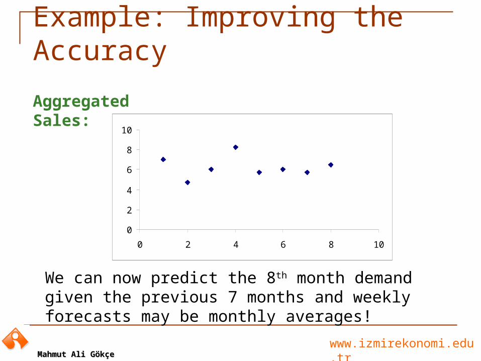
Aggregated Sales:
www.izmirekonomi.edu.trMahmut Ali GökçeMahmut Ali Gökçe
Example: Improving the Accuracy
Aggregated Sales:
We can now predict the 8th month demand given the previous 7 months and weekly forecasts may be monthly averages!
0
2
4
6
8
10
0 2 4 6 8 10
www.izmirekonomi.edu.trMahmut Ali GökçeMahmut Ali Gökçe
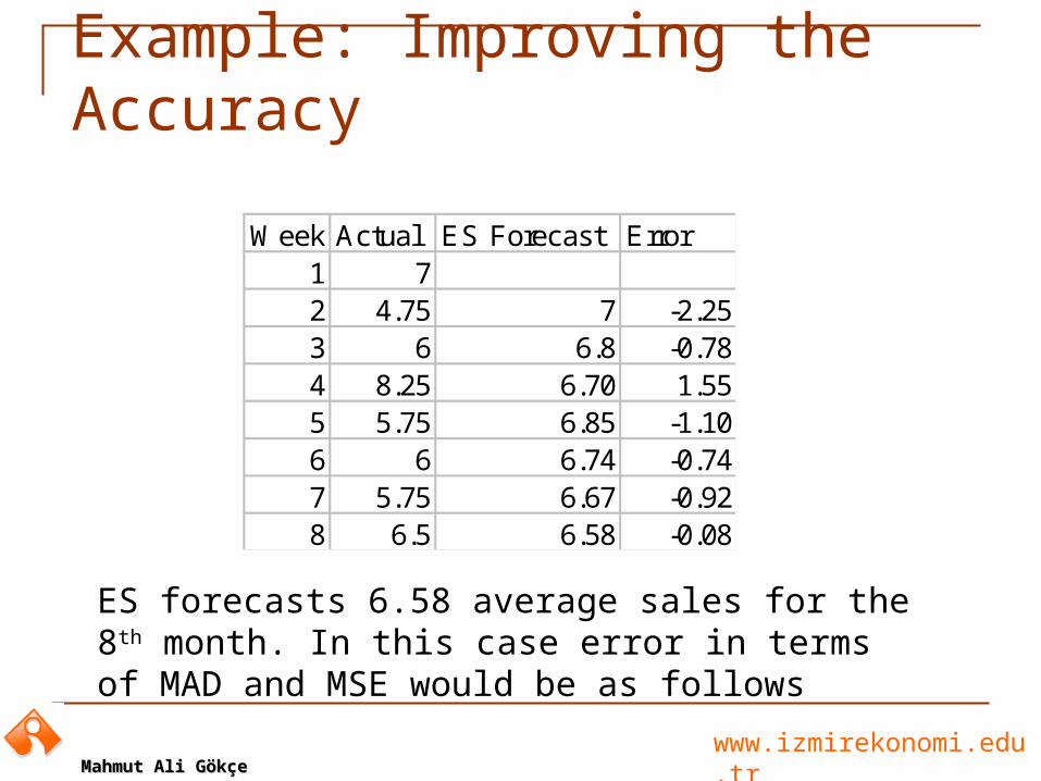
Example: Improving the Accuracy
ES forecasts 6.58 average sales for the 8th month. In this case error in terms of MAD and MSE would be as follows
Week Actual ES Forecast Error1 72 4.75 7 -2.253 6 6.8 -0.784 8.25 6.70 1.555 5.75 6.85 -1.106 6 6.74 -0.747 5.75 6.67 -0.928 6.5 6.58 -0.08
www.izmirekonomi.edu.trMahmut Ali GökçeMahmut Ali Gökçe
Example: Improving the Accuracy
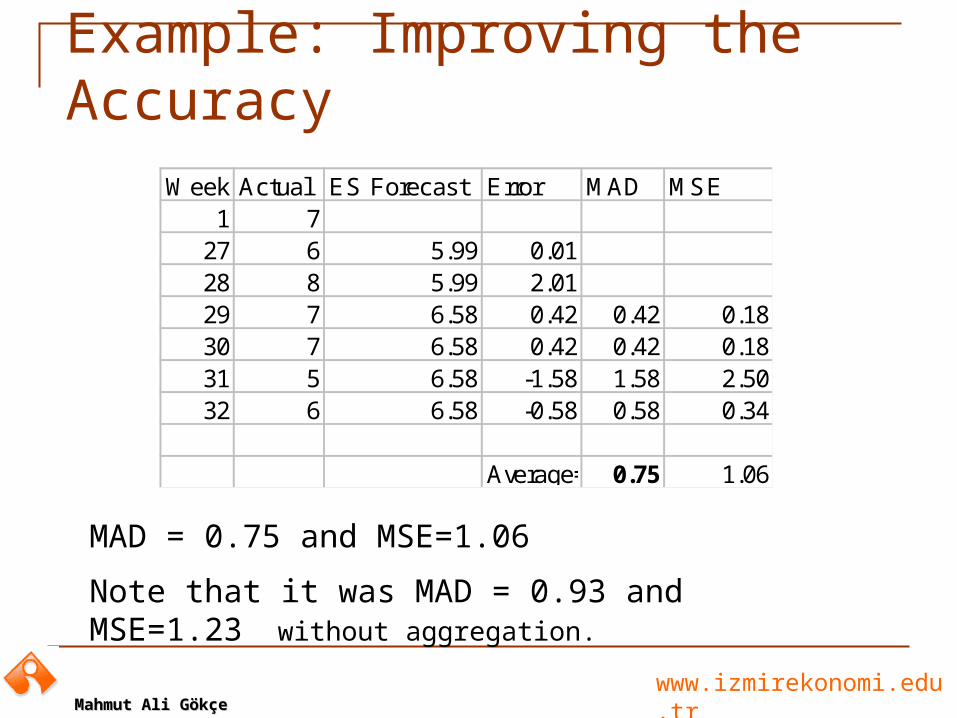
MAD = 0.75 and MSE=1.06
Note that it was MAD = 0.93 and MSE=1.23 without aggregation.
Week Actual ES Forecast Error MAD MSE1 7
27 6 5.99 0.0128 8 5.99 2.0129 7 6.58 0.42 0.42 0.1830 7 6.58 0.42 0.42 0.1831 5 6.58 -1.58 1.58 2.5032 6 6.58 -0.58 0.58 0.34
Average= 0.75 1.06
www.izmirekonomi.edu.trMahmut Ali GökçeMahmut Ali Gökçe
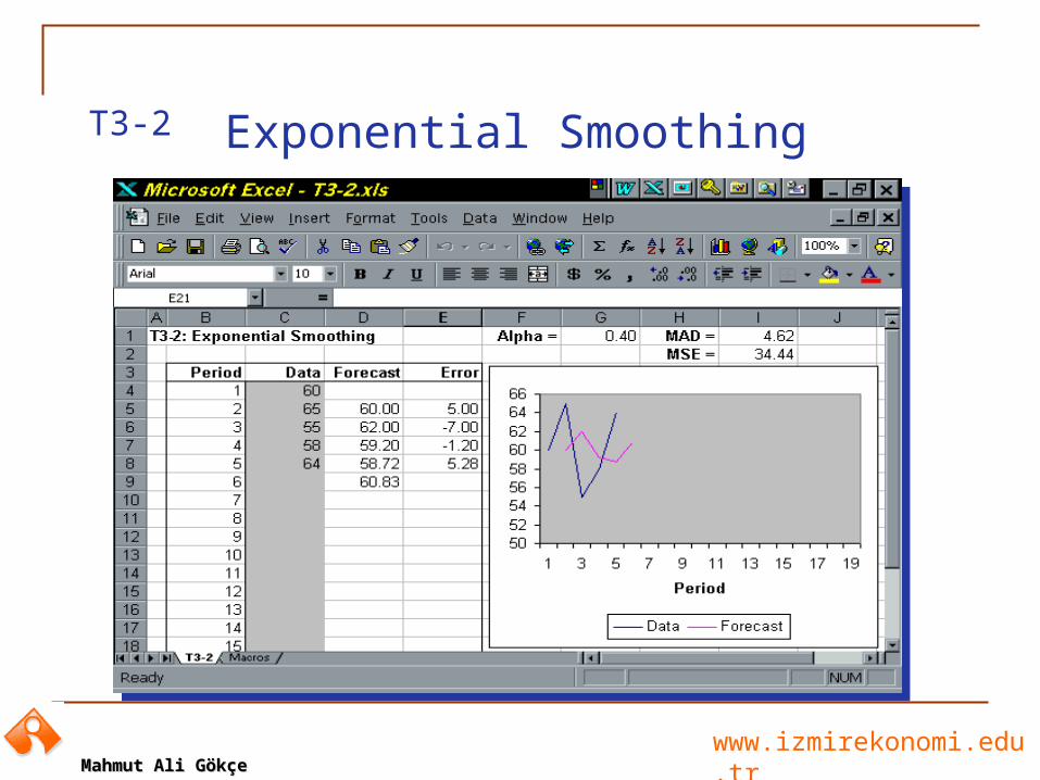
Exponential SmoothingT3-2
www.izmirekonomi.edu.trMahmut Ali GökçeMahmut Ali Gökçe
Linear Trend EquationT3-3
www.izmirekonomi.edu.trMahmut Ali GökçeMahmut Ali Gökçe
Trend Adjusted Exponential SmoothingT3-4
www.izmirekonomi.edu.trMahmut Ali GökçeMahmut Ali Gökçe
Simple Linear RegressionT3-5
www.izmirekonomi.edu.trMahmut Ali GökçeMahmut Ali Gökçe
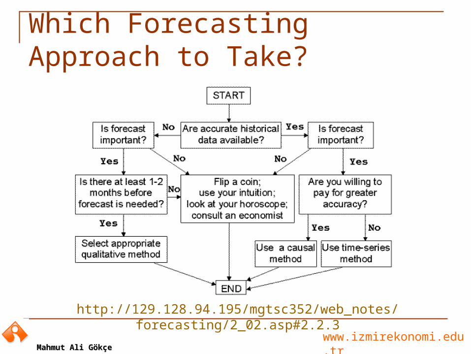
Which Forecasting Approach to Take?
http://129.128.94.195/mgtsc352/web_notes/forecasting/2_02.asp#2.2.3
www.izmirekonomi.edu.trMahmut Ali GökçeMahmut Ali Gökçe
Resources
Textbooks!
http://129.128.94.195/mgtsc352/web_notes/forecasting/toc.asp (MGTSC 352)
http://www.itl.nist.gov/div898/handbook/pmc/section4/pmc4.htm