Embed Size (px)
Citation preview
Spiking Neuron ModelsSingle Neurons, Populations, Plasticity
Wulfram Gerstner and Werner M. Kistler
Cambridge University Press, 2002

2
Preface
The task of understanding the principles of information processing in the brain poses,apart from numerous experimental questions, challenging theoretical problems on alllevels from molecules to behavior. This books concentrates on modeling approacheson the level of neurons and small populations of neurons, since we think that this isan appropriate level to adress fundamental questions of neuronal coding, signal trans-mission, or synaptic plasticity. In this text we concentrate on theoretical conceptsand phenomenological models derived from them. We think of a neuron primarilyas a dynamic element that emits output pulses whenever the excitation exceeds somethreshold. The resulting sequence of pulses or ‘spikes’ contains all the information thatis transmitted from one neuron to the next. In order to understand signal transmissionand signal processing in neuronal systems, we need an understanding of their basicelements, i.e., the neurons, which is the topic of part I. New phenomena emerge whenseveral neurons are coupled. Part II introduces network concepts, in particular patternformation, collective excitations, and rapid signal transmission between neuronal pop-ulations. Learning concepts presented in Part III are based on spike-time dependentsynaptic plasticity.
We wrote this book as an introduction to spiking neuron models for advancedundergraduate or graduate students. It can be used either as the main text for a coursethat focuses on neuronal dynamics; or as part of a larger course in ComputationalNeuroscience, theoretical biology, neuronal modeling, biophysics, or neural networks.For a one-semester course on neuronal modeling, we usually teach one chapter perweek focusing on the first sections of each chapter for lectures and give the remainderas reading assignment. Many of the examples can be adapted to become exercises orprojects for students. While writing the book we had in mind students of physics,mathematics, or computer science with an interest in biology; but it might also beuseful for students of biology who are interested in mathematical modeling. All thenecessary mathematical concepts are introduced in an elementary fashion, and we haveprovided many illustrative figures which complement the mathematical analysis andhelp the reader picture what is going on. No prior knowledge beyond undergraduatemathematics should be necessary to read the book. An asterix (*) marks those sectionsthat have a more mathematical focus. These sections can be skipped at a first reading.
We have also tried to keep the book self-contained with respect to the underlyingNeurobiology. The fundamentals of neuronal excitation and synaptic signal transmis-sion are briefly introduced in Chapter 1 together with an outlook on the principal topicsof the book, viz., formal spiking neuron models and the problem of neuronal coding.In Chapter 2 we review biophysical models, such as the Hodgkin-Huxley equations ofneuronal dynamics, and models of dendritic integration based on the cable equation.These are the starting point for a systematic reduction to neuron models with a reducedcomplexity that are open to an analytical treatment. Whereas Chapter 3 is dedicatedto two-dimensional differential equations as a description of neuronal dynamics, Chap-ter 4 introduces formal spiking neuron models, namely the integrate-and-fire model andthe Spike Response Model. These formal neuron models are the foundation for all thefollowing chapters. Part I on “Single Neuron Models” is rounded off by Chapter 5 which
gives an overview of spike-train statistics and illustrates how noise can be implementedin spiking neuron models.
The step from single neuron models to networks of neurons is taken in Chapter6 where equations for the macroscopic dynamics of large populations of neurons arederived. Based on these equations phenomena like signal transmission and coding(Chapter 7), oscillations and synchrony (Chapter 8), and pattern formation in spatiallystructured networks (Chapter 9) are investigated. Up to this point, only networks witha fixed synaptic connectivity have been discussed. The third part of the book, finally,deals with synaptic plasticity and its role for development, learning, and memory.In Chapter 10, principles of Hebbian plasticity are presented and various models ofsynaptic plasticity are described that are more or less directly inspired by neurbiologicalfindings. Equations that relate the synaptic weight dynamics to statistical propertiesof the neuronal spike activity are derived in Chapter 11. Last but not least, Chapter 12presents an – admittedly personal – choice of illustrative applications of spike-timingdependent synaptic plasticity to fundamental problems of neuronal coding.
While the book contains material which is now considered as standard for coursesof the type mentioned earlier, it also provides a bridge to current research which hasdeveloped over the last few years. In most chapters, the reader will find some sectionswhich either report recent results or shed new light on well-known models. The view-point taken in the presentation of the material is of course highly subjective and a biastowards our own research is obvious. Nevertheless, we hope that the book will find theinterest of students and researchers in the field.
Werner M. KistlerWulfram Gerstner
Lausanne, November 2001
Acknowledgments
This book would not have been possible without the help of our friends and colleagueswho made many valuable comments and spotted numerous mistakes. In particular, wewould like to thank Silvio Borer, Nicolas Brunel, Stefano Fusi, Evan Haskell, AndreasHerz, Renaud Jolivet, Maurizio Mattia, Jean-Pascal Pfister, Hans-Ekkehard Plesser,Marc van Rossum, Walter Senn, and Arnaud Tonnelier for a careful reading of thetext. We owe special thanks to Leo van Hemmen who encouraged us to write a bookon our joint work. Even though the scope of the text has changed over the years,the original initiative is due to him. Finally, we thank all the students who attendedtutorials or classes taught by us and whose critical comments helped us to organize ourthoughts.
W.G. and W.M.K.
Contents
1 Introduction 111.1 Elements of Neuronal Systems . . . . . . . . . . . . . . . . . . . . 11
1.1.1 The Ideal Spiking Neuron . . . . . . . . . . . . . . . . . . 121.1.2 Spike Trains . . . . . . . . . . . . . . . . . . . . . . . . . . 131.1.3 Synapses . . . . . . . . . . . . . . . . . . . . . . . . . . . . 14
1.2 Elements of Neuronal Dynamics . . . . . . . . . . . . . . . . . . . 141.2.1 Postsynaptic Potentials . . . . . . . . . . . . . . . . . . . . 141.2.2 Firing Threshold and Action Potential . . . . . . . . . . . 15
1.3 A Phenomenological Neuron Model . . . . . . . . . . . . . . . . . 151.3.1 Definition of the Model SRM0 . . . . . . . . . . . . . . . . 171.3.2 Limitations of the Model . . . . . . . . . . . . . . . . . . . 19
1.4 The Problem of Neuronal Coding . . . . . . . . . . . . . . . . . . 231.5 Rate Codes . . . . . . . . . . . . . . . . . . . . . . . . . . . . . . 25
1.5.1 Rate as a Spike Count (Average over Time) . . . . . . . . 251.5.2 Rate as a Spike Density (Average over Several Runs) . . . 271.5.3 Rate as a Population Activity (Average over Several Neurons) 28
1.6 Spike Codes . . . . . . . . . . . . . . . . . . . . . . . . . . . . . . 291.6.1 Time-to-First-Spike . . . . . . . . . . . . . . . . . . . . . . 291.6.2 Phase . . . . . . . . . . . . . . . . . . . . . . . . . . . . . 311.6.3 Correlations and Synchrony . . . . . . . . . . . . . . . . . 311.6.4 Stimulus Reconstruction and Reverse Correlation . . . . . 32
1.7 Discussion: Spikes or Rates? . . . . . . . . . . . . . . . . . . . . . 341.8 Summary . . . . . . . . . . . . . . . . . . . . . . . . . . . . . . . 37
I Single Neuron Models 39
2 Detailed Neuron Models 412.1 Equilibrium potential . . . . . . . . . . . . . . . . . . . . . . . . . 41
2.1.1 Nernst potential . . . . . . . . . . . . . . . . . . . . . . . . 412.1.2 Reversal Potential . . . . . . . . . . . . . . . . . . . . . . . 43
2.2 Hodgkin-Huxley Model . . . . . . . . . . . . . . . . . . . . . . . . 44
5
6 CONTENTS
2.2.1 Definition of the model . . . . . . . . . . . . . . . . . . . . 442.2.2 Dynamics . . . . . . . . . . . . . . . . . . . . . . . . . . . 46
2.3 The Zoo of Ion Channels . . . . . . . . . . . . . . . . . . . . . . . 512.3.1 Sodium Channels . . . . . . . . . . . . . . . . . . . . . . . 512.3.2 Potassium Channels . . . . . . . . . . . . . . . . . . . . . 532.3.3 Low-Threshold Calcium Current . . . . . . . . . . . . . . . 552.3.4 High-threshold calcium current and Ca2+-Activated Potas-
sium Channels . . . . . . . . . . . . . . . . . . . . . . . . . 572.3.5 Calcium Dynamics . . . . . . . . . . . . . . . . . . . . . . 60
2.4 Synapses . . . . . . . . . . . . . . . . . . . . . . . . . . . . . . . . 612.4.1 Inhibitory Synapses . . . . . . . . . . . . . . . . . . . . . . 612.4.2 Excitatory Synapses . . . . . . . . . . . . . . . . . . . . . 62
2.5 Spatial Structure: The Dendritic Tree . . . . . . . . . . . . . . . . 632.5.1 Derivation of the Cable Equation . . . . . . . . . . . . . . 642.5.2 Green’s Function (*) . . . . . . . . . . . . . . . . . . . . . 672.5.3 Non-linear Extensions to the Cable Equation . . . . . . . . 69
2.6 Compartmental Models . . . . . . . . . . . . . . . . . . . . . . . . 712.7 Summary . . . . . . . . . . . . . . . . . . . . . . . . . . . . . . . 75
3 Two-Dimensional Neuron Models 773.1 Reduction to two dimensions . . . . . . . . . . . . . . . . . . . . . 77
3.1.1 General approach . . . . . . . . . . . . . . . . . . . . . . . 773.1.2 Mathematical steps (*) . . . . . . . . . . . . . . . . . . . . 80
3.2 Phase plane analysis . . . . . . . . . . . . . . . . . . . . . . . . . 823.2.1 Nullclines . . . . . . . . . . . . . . . . . . . . . . . . . . . 823.2.2 Stability of Fixed Points . . . . . . . . . . . . . . . . . . . 833.2.3 Limit cycles . . . . . . . . . . . . . . . . . . . . . . . . . . 853.2.4 Type I and type II models . . . . . . . . . . . . . . . . . . 88
3.3 Threshold and excitability . . . . . . . . . . . . . . . . . . . . . . 913.3.1 Type I models . . . . . . . . . . . . . . . . . . . . . . . . . 923.3.2 Type II models . . . . . . . . . . . . . . . . . . . . . . . . 933.3.3 Separation of time scales . . . . . . . . . . . . . . . . . . . 94
3.4 Summary . . . . . . . . . . . . . . . . . . . . . . . . . . . . . . . 99
4 Formal Spiking Neuron Models 1014.1 Integrate-and-fire model . . . . . . . . . . . . . . . . . . . . . . . 101
4.1.1 Leaky Integrate-and-Fire Model . . . . . . . . . . . . . . . 1024.1.2 Nonlinear integrate-and-fire model . . . . . . . . . . . . . 1054.1.3 Stimulation by Synaptic Currents . . . . . . . . . . . . . . 108
4.2 Spike response model (SRM) . . . . . . . . . . . . . . . . . . . . . 1104.2.1 Definition of the SRM . . . . . . . . . . . . . . . . . . . . 1104.2.2 Mapping the Integrate-and-Fire Model to the SRM . . . . 116
CONTENTS 7
4.2.3 Simplified Model SRM0 . . . . . . . . . . . . . . . . . . . . 119
4.3 From Detailed Models to Formal Spiking Neurons . . . . . . . . . 124
4.3.1 Reduction of the Hodgkin-Huxley Model . . . . . . . . . . 125
4.3.2 Reduction of a Cortical Neuron Model . . . . . . . . . . . 132
4.3.3 Limitations . . . . . . . . . . . . . . . . . . . . . . . . . . 142
4.4 Multi-compartment integrate-and-fire model . . . . . . . . . . . . 142
4.4.1 Definition of the Model . . . . . . . . . . . . . . . . . . . . 143
4.4.2 Relation to the Model SRM0 . . . . . . . . . . . . . . . . . 144
4.4.3 Relation to the Full Spike Response Model (*) . . . . . . . 146
4.5 Application: Coding by Spikes . . . . . . . . . . . . . . . . . . . . 149
4.6 Summary . . . . . . . . . . . . . . . . . . . . . . . . . . . . . . . 154
5 Noise in Spiking Neuron Models 157
5.1 Spike train variability . . . . . . . . . . . . . . . . . . . . . . . . . 158
5.1.1 Are neurons noisy? . . . . . . . . . . . . . . . . . . . . . . 158
5.1.2 Noise sources . . . . . . . . . . . . . . . . . . . . . . . . . 159
5.2 Statistics of spike trains . . . . . . . . . . . . . . . . . . . . . . . 160
5.2.1 Input-dependent renewal systems . . . . . . . . . . . . . . 160
5.2.2 Interval distribution . . . . . . . . . . . . . . . . . . . . . 162
5.2.3 Survivor function and hazard . . . . . . . . . . . . . . . . 163
5.2.4 Stationary renewal theory and experiments . . . . . . . . . 167
5.2.5 Autocorrelation of a stationary renewal process . . . . . . 170
5.3 Escape noise . . . . . . . . . . . . . . . . . . . . . . . . . . . . . . 174
5.3.1 Escape rate and hazard function . . . . . . . . . . . . . . . 174
5.3.2 Interval distribution and mean firing rate . . . . . . . . . . 178
5.4 Slow noise in the parameters . . . . . . . . . . . . . . . . . . . . . 182
5.5 Diffusive noise . . . . . . . . . . . . . . . . . . . . . . . . . . . . . 184
5.5.1 Stochastic spike arrival . . . . . . . . . . . . . . . . . . . . 184
5.5.2 Diffusion limit (*) . . . . . . . . . . . . . . . . . . . . . . . 188
5.5.3 Interval distribution . . . . . . . . . . . . . . . . . . . . . 192
5.6 The subthreshold regime . . . . . . . . . . . . . . . . . . . . . . . 194
5.6.1 Sub- and superthreshold stimulation . . . . . . . . . . . . 195
5.6.2 Coefficient of variation CV . . . . . . . . . . . . . . . . . . 196
5.7 From diffusive noise to escape noise . . . . . . . . . . . . . . . . . 198
5.8 Stochastic resonance . . . . . . . . . . . . . . . . . . . . . . . . . 200
5.9 Stochastic firing and rate models . . . . . . . . . . . . . . . . . . 203
5.9.1 Analog neurons . . . . . . . . . . . . . . . . . . . . . . . . 204
5.9.2 Stochastic rate model . . . . . . . . . . . . . . . . . . . . . 205
5.9.3 Population rate model . . . . . . . . . . . . . . . . . . . . 207
5.10 Summary . . . . . . . . . . . . . . . . . . . . . . . . . . . . . . . 208
8 CONTENTS
II Population Models 211
6 Population Equations 2136.1 Fully Connected Homogeneous Network . . . . . . . . . . . . . . . 2146.2 Density Equations . . . . . . . . . . . . . . . . . . . . . . . . . . 217
6.2.1 Integrate-and-Fire Neurons with Stochastic Spike Arrival . 2176.2.2 Spike Response Model Neurons with Escape Noise . . . . . 2236.2.3 Relation between the Approaches . . . . . . . . . . . . . . 227
6.3 Integral Equations for the Population Activity . . . . . . . . . . . 2326.3.1 Assumptions . . . . . . . . . . . . . . . . . . . . . . . . . . 2336.3.2 Integral equation for the dynamics . . . . . . . . . . . . . 233
6.4 Asynchronous firing . . . . . . . . . . . . . . . . . . . . . . . . . . 2406.4.1 Stationary Activity and Mean Firing Rate . . . . . . . . . 2416.4.2 Gain Function and Fixed Points of the Activity . . . . . . 2436.4.3 Low-Connectivity Networks . . . . . . . . . . . . . . . . . 246
6.5 Interacting Populations and Continuum Models . . . . . . . . . . 2506.5.1 Several Populations . . . . . . . . . . . . . . . . . . . . . . 2506.5.2 Spatial Continuum Limit . . . . . . . . . . . . . . . . . . . 252
6.6 Limitations . . . . . . . . . . . . . . . . . . . . . . . . . . . . . . 2546.7 Summary . . . . . . . . . . . . . . . . . . . . . . . . . . . . . . . 256
7 Signal Transmission and Neuronal Coding 2577.1 Linearized Population Equation . . . . . . . . . . . . . . . . . . . 258
7.1.1 Noise-free Population Dynamics (*) . . . . . . . . . . . . . 2597.1.2 Escape noise (*) . . . . . . . . . . . . . . . . . . . . . . . . 2637.1.3 Noisy reset (*) . . . . . . . . . . . . . . . . . . . . . . . . 268
7.2 Transients . . . . . . . . . . . . . . . . . . . . . . . . . . . . . . . 2697.2.1 Transients in a Noise-Free Network . . . . . . . . . . . . . 2707.2.2 Transients with Noise . . . . . . . . . . . . . . . . . . . . . 272
7.3 Transfer Function . . . . . . . . . . . . . . . . . . . . . . . . . . . 2767.3.1 Signal Term . . . . . . . . . . . . . . . . . . . . . . . . . . 2767.3.2 Signal-to-Noise Ratio . . . . . . . . . . . . . . . . . . . . . 280
7.4 The Significance of a Single Spike . . . . . . . . . . . . . . . . . . 2817.4.1 The Effect of an Input Spike . . . . . . . . . . . . . . . . . 2817.4.2 Reverse Correlation - the Significance of an Output Spike . 286
7.5 Summary . . . . . . . . . . . . . . . . . . . . . . . . . . . . . . . 290
8 Oscillations and Synchrony 2938.1 Instability of the Asynchronous State . . . . . . . . . . . . . . . . 2948.2 Synchronized Oscillations and Locking . . . . . . . . . . . . . . . 300
8.2.1 Locking in Noise-Free Populations . . . . . . . . . . . . . . 3008.2.2 Locking in SRM0 Neurons with Noisy Reset (*) . . . . . . 306
CONTENTS 9
8.2.3 Cluster States . . . . . . . . . . . . . . . . . . . . . . . . . 308
8.3 Oscillations in reverberating loops . . . . . . . . . . . . . . . . . . 310
8.3.1 From oscillations with spiking neurons to binary neurons . 313
8.3.2 Mean field dynamics . . . . . . . . . . . . . . . . . . . . . 313
8.3.3 Microscopic dynamics . . . . . . . . . . . . . . . . . . . . 317
8.4 Summary . . . . . . . . . . . . . . . . . . . . . . . . . . . . . . . 321
9 Spatially Structured Networks 323
9.1 Stationary patterns of neuronal activity . . . . . . . . . . . . . . . 324
9.1.1 Homogeneous solutions . . . . . . . . . . . . . . . . . . . . 325
9.1.2 Stability of homogeneous states . . . . . . . . . . . . . . . 327
9.1.3 ‘Blobs’ of activity: inhomogeneous states . . . . . . . . . . 331
9.2 Dynamic patterns of neuronal activity . . . . . . . . . . . . . . . 337
9.2.1 Oscillations . . . . . . . . . . . . . . . . . . . . . . . . . . 338
9.2.2 Traveling waves . . . . . . . . . . . . . . . . . . . . . . . . 340
9.3 Patterns of spike activity . . . . . . . . . . . . . . . . . . . . . . . 342
9.3.1 Traveling fronts and waves (*) . . . . . . . . . . . . . . . . 345
9.3.2 Stability (*) . . . . . . . . . . . . . . . . . . . . . . . . . . 347
9.4 Robust transmission of temporal information . . . . . . . . . . . . 349
9.5 Summary . . . . . . . . . . . . . . . . . . . . . . . . . . . . . . . 357
III Models of Synaptic Plasticity 359
10 Hebbian Models 361
10.1 Synaptic Plasticity . . . . . . . . . . . . . . . . . . . . . . . . . . 361
10.1.1 Long-Term Potentiation . . . . . . . . . . . . . . . . . . . 362
10.1.2 Temporal Aspects . . . . . . . . . . . . . . . . . . . . . . . 364
10.2 Rate-Based Hebbian Learning . . . . . . . . . . . . . . . . . . . . 366
10.2.1 A Mathematical Formulation of Hebb’s Rule . . . . . . . . 366
10.3 Spike-Time Dependent Plasticity . . . . . . . . . . . . . . . . . . 371
10.3.1 Phenomenological Model . . . . . . . . . . . . . . . . . . . 372
10.3.2 Consolidation of Synaptic Efficacies . . . . . . . . . . . . . 375
10.3.3 General Framework (*) . . . . . . . . . . . . . . . . . . . . 376
10.4 Detailed Models of Synaptic Plasticity . . . . . . . . . . . . . . . 380
10.4.1 A Simple Mechanistic Model . . . . . . . . . . . . . . . . . 380
10.4.2 A Kinetic Model based on NMDA Receptors . . . . . . . . 383
10.4.3 A Calcium-Based Model . . . . . . . . . . . . . . . . . . . 387
10.5 Summary . . . . . . . . . . . . . . . . . . . . . . . . . . . . . . . 392
10 CONTENTS
11 Learning Equations 39511.1 Learning in Rate Models . . . . . . . . . . . . . . . . . . . . . . . 395
11.1.1 Correlation Matrix and Principal Components . . . . . . . 39511.1.2 Evolution of synaptic weights . . . . . . . . . . . . . . . . 39711.1.3 Weight Normalization . . . . . . . . . . . . . . . . . . . . 40211.1.4 Receptive Field Development . . . . . . . . . . . . . . . . 406
11.2 Learning in Spiking Models . . . . . . . . . . . . . . . . . . . . . 41211.2.1 Learning Equation . . . . . . . . . . . . . . . . . . . . . . 41211.2.2 Spike-Spike Correlations . . . . . . . . . . . . . . . . . . . 41511.2.3 Relation of spike-based to rate-based learning . . . . . . . 41711.2.4 Static-Pattern Scenario . . . . . . . . . . . . . . . . . . . . 42011.2.5 Distribution of Synaptic Weights . . . . . . . . . . . . . . 423
11.3 Summary . . . . . . . . . . . . . . . . . . . . . . . . . . . . . . . 426
12 Plasticity and Coding 42912.1 Learning to be Fast . . . . . . . . . . . . . . . . . . . . . . . . . . 42912.2 Learning to be Precise . . . . . . . . . . . . . . . . . . . . . . . . 433
12.2.1 The Model . . . . . . . . . . . . . . . . . . . . . . . . . . . 43312.2.2 Firing time distribution . . . . . . . . . . . . . . . . . . . 43512.2.3 Stationary Synaptic Weights . . . . . . . . . . . . . . . . . 43612.2.4 The Role of the Firing Threshold . . . . . . . . . . . . . . 438
12.3 Sequence Learning . . . . . . . . . . . . . . . . . . . . . . . . . . 44112.4 Subtraction of Expectations . . . . . . . . . . . . . . . . . . . . . 445
12.4.1 Electro-Sensory System of Mormoryd Electric Fish . . . . 44512.4.2 Sensory Image Cancellation . . . . . . . . . . . . . . . . . 447
12.5 Transmission of Temporal Codes . . . . . . . . . . . . . . . . . . . 45012.5.1 Auditory Pathway and Sound Source Localization . . . . . 45012.5.2 Phase Locking and Coincidence Detection . . . . . . . . . 45312.5.3 Tuning of Delay Lines . . . . . . . . . . . . . . . . . . . . 455
Chapter 1
Introduction
The aim of this chapter is to introduce several elementary notions of neuro-science, in particular the concepts of action potentials, postsynaptic potentials,firing thresholds, and refractoriness. Based on these notions a first phenomeno-logical model of neuronal dynamics is built that will be used as a starting pointfor a discussion of neuronal coding. Due to the limitations of space we cannot –and do not want to – give a comprehensive introduction into such a complex fieldas neurobiology. The presentation of the biological background in this chapter istherefore highly selective and simplistic. For an in-depth discussion of neurobi-ology we refer the reader to the literature mentioned at the end of this chapter.Nevertheless, we try to provide the reader with a minimum of information nec-essary to appreciate the biological background of the theoretical work presentedin this book.
1.1 Elements of Neuronal Systems
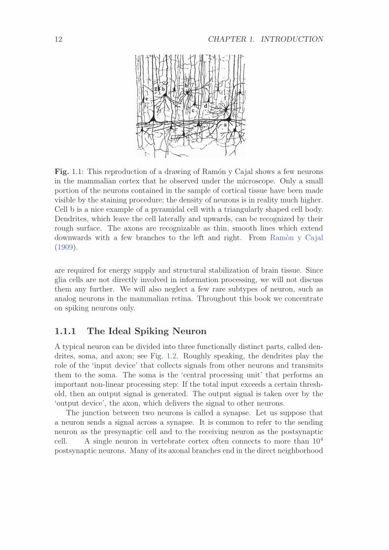
Over the past hundred years, biological research has accumulated an enormousamount of detailed knowledge about the structure and function of the brain. Theelementary processing units in the central nervous system are neurons which areconnected to each other in an intricate pattern. A tiny portion of such a networkof neurons is sketched in Fig. 1.1 which shows a drawing by Ramon y Cajal, oneof the pioneers of neuroscience around 1900. We can distinguish several neuronswith triangular or circular cell bodies and long wire-like extensions. This picturecan only give a glimpse of the network of neurons in the cortex. In reality, corticalneurons and their connections are packed into a dense network with more than104 cell bodies and several kilometers of ‘wires’ per cubic millimeter. In otherareas of the brain the wiring pattern may look different. In all areas, however,neurons of different sizes and shapes form the basic elements.
The cortex does not consist exclusively of neurons. Beside the various typesof neuron there is a large number of ‘supporter’ cells, so-called glia cells, that
11
12 CHAPTER 1. INTRODUCTION
Fig. 1.1: This reproduction of a drawing of Ramon y Cajal shows a few neuronsin the mammalian cortex that he observed under the microscope. Only a smallportion of the neurons contained in the sample of cortical tissue have been madevisible by the staining procedure; the density of neurons is in reality much higher.Cell b is a nice example of a pyramidal cell with a triangularly shaped cell body.Dendrites, which leave the cell laterally and upwards, can be recognized by theirrough surface. The axons are recognizable as thin, smooth lines which extenddownwards with a few branches to the left and right. From Ramon y Cajal(1909).
are required for energy supply and structural stabilization of brain tissue. Sinceglia cells are not directly involved in information processing, we will not discussthem any further. We will also neglect a few rare subtypes of neuron, such asanalog neurons in the mammalian retina. Throughout this book we concentrateon spiking neurons only.
1.1.1 The Ideal Spiking Neuron
A typical neuron can be divided into three functionally distinct parts, called den-drites, soma, and axon; see Fig. 1.2. Roughly speaking, the dendrites play therole of the ‘input device’ that collects signals from other neurons and transmitsthem to the soma. The soma is the ‘central processing unit’ that performs animportant non-linear processing step: If the total input exceeds a certain thresh-old, then an output signal is generated. The output signal is taken over by the‘output device’, the axon, which delivers the signal to other neurons.
The junction between two neurons is called a synapse. Let us suppose thata neuron sends a signal across a synapse. It is common to refer to the sendingneuron as the presynaptic cell and to the receiving neuron as the postsynapticcell. A single neuron in vertebrate cortex often connects to more than 104
postsynaptic neurons. Many of its axonal branches end in the direct neighborhood
1.1. ELEMENTS OF NEURONAL SYSTEMS 13
A B
1 ms10 mV
actionpotential
dendrites
soma
electrode
axon
dendrites
axon
synapse
j
i
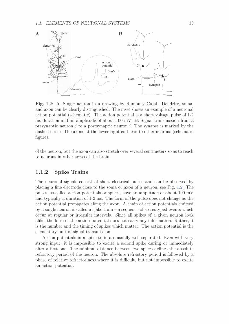
Fig. 1.2: A. Single neuron in a drawing by Ramon y Cajal. Dendrite, soma,and axon can be clearly distinguished. The inset shows an example of a neuronalaction potential (schematic). The action potential is a short voltage pulse of 1-2ms duration and an amplitude of about 100 mV. B. Signal transmission from apresynaptic neuron j to a postsynaptic neuron i. The synapse is marked by thedashed circle. The axons at the lower right end lead to other neurons (schematicfigure).
of the neuron, but the axon can also stretch over several centimeters so as to reachto neurons in other areas of the brain.
1.1.2 Spike Trains
The neuronal signals consist of short electrical pulses and can be observed byplacing a fine electrode close to the soma or axon of a neuron; see Fig. 1.2. Thepulses, so-called action potentials or spikes, have an amplitude of about 100 mVand typically a duration of 1-2 ms. The form of the pulse does not change as theaction potential propagates along the axon. A chain of action potentials emittedby a single neuron is called a spike train – a sequence of stereotyped events whichoccur at regular or irregular intervals. Since all spikes of a given neuron lookalike, the form of the action potential does not carry any information. Rather, itis the number and the timing of spikes which matter. The action potential is theelementary unit of signal transmission.
Action potentials in a spike train are usually well separated. Even with verystrong input, it is impossible to excite a second spike during or immediatelyafter a first one. The minimal distance between two spikes defines the absoluterefractory period of the neuron. The absolute refractory period is followed by aphase of relative refractoriness where it is difficult, but not impossible to excitean action potential.
14 CHAPTER 1. INTRODUCTION
1.1.3 Synapses
The site where the axon of a presynaptic neuron makes contact with the den-drite (or soma) of a postsynaptic cell is the synapse. The most common type ofsynapse in the vertebrate brain is a chemical synapse. At a chemical synapse,the axon terminal comes very close to the postsynaptic neuron, leaving only atiny gap between pre- and postsynaptic cell membrane, called the synaptic cleft.When an action potential arrives at a synapse, it triggers a complex chain ofbio-chemical processing steps that lead to a release of neurotransmitter from thepresynaptic terminal into the synaptic cleft. As soon as transmitter moleculeshave reached the postsynaptic side, they will be detected by specialized receptorsin the postsynaptic cell membrane and open (either directly or via a biochemicalsignaling chain) specific channels so that ions from the extracellular fluid flowinto the cell. The ion influx, in turn, leads to a change of the membrane poten-tial at the postsynaptic site so that, in the end, the chemical signal is translatedinto an electrical response. The voltage response of the postsynaptic neuron to apresynaptic action potential is called the postsynaptic potential.
Apart from chemical synapses neurons can also be coupled by electrical synap-ses, so-called gap junctions. Specialized membrane proteins make a direct elec-trical connection between the two neurons. Not very much is known about thefunctional aspects of gap junctions, but they are thought to be involved in thesynchronization of neurons.
1.2 Elements of Neuronal Dynamics
The effect of a spike on the postsynaptic neuron can be recorded with an intracel-lular electrode which measures the potential difference u(t) between the interiorof the cell and its surroundings. This potential difference is called the membranepotential. Without any spike input, the neuron is at rest corresponding to a con-stant membrane potential. After the arrival of a spike, the potential changes andfinally decays back to the resting potential, cf. Fig. 1.3A. If the change is posi-tive, the synapse is said to be excitatory. If the change is negative, the synapseis inhibitory.
At rest, the cell membrane has already a strong negative polarization of about-65mV. An input at an excitatory synapse reduces the negative polarization ofthe membrane and is therefore called depolarizing. An input that increases thenegative polarization of the membrane even further is called hyperpolarizing.
1.2.1 Postsynaptic Potentials
Let us formalize the above observation. We study the time course ui(t) of themembrane potential of neuron i. Before the input spike has arrived, we have
1.3. A PHENOMENOLOGICAL NEURON MODEL 15
ui(t) = urest. At t = 0 the presynaptic neuron j fires its spike. For t > 0, we seeat the electrode a response of neuron i
ui(t)− urest =: εij(t) . (1.1)
The right-hand side of Eq. (1.1) defines the postsynaptic potential (PSP). Ifthe voltage difference ui(t) − urest is positive (negative) we have an excitatory(inhibitory) postsynaptic potential or short EPSP (IPSP). In Fig. 1.3A we havesketched the EPSP caused by the arrival of a spike from neuron j at an excitatorysynapse of neuron i.
1.2.2 Firing Threshold and Action Potential
Consider two presynaptic neurons j = 1, 2, which both send spikes to the post-synaptic neuron i. Neuron j = 1 fires spikes at t
(1)1 , t
(2)1 , . . . , similarly neuron
j = 2 fires at t(1)2 , t
(2)2 , . . . . Each spike evokes a postsynaptic potential εi1 or εi2,
respectively. As long as there are only few input spikes, the total change of thepotential is approximately the sum of the individual PSPs,
ui(t) =∑
j
∑f
εij(t− t(f)j ) + urest , (1.2)
i.e., the membrane potential responds linearly to input spikes; see Fig. 1.3B.On the other hand, linearity breaks down if too many input spikes arrive
during a short interval. As soon as the membrane potential reaches a criticalvalue ϑ, its trajectory shows a behavior that is quite different from a simplesummation of PSPs: The membrane potential exhibits a pulse-like excursion withan amplitude of about 100 mV, viz., an action potential. This action potentialwill propagate along the axon of neuron i to the synapses of other neurons. Afterthe pulse the membrane potential does not directly return to the resting potential,but passes through a phase of hyperpolarization below the resting value. Thishyperpolarization is called ‘spike-afterpotential’.
Single EPSPs have amplitudes in the range of one millivolt. The criticalvalue for spike initiation is about 20 to 30 mV above the resting potential. Inmost neurons, four spikes – as shown schematically in Fig. 1.3C – are thus notsufficient to trigger an action potential. Instead, about 20-50 presynaptic spikeshave to arrive within a short time window before postsynaptic action potentialsare triggered.
1.3 A Phenomenological Neuron Model
In order to build a phenomenological model of neuronal dynamics, we describethe critical voltage for spike initiation by a formal threshold ϑ. If ui(t) reaches ϑ
16 CHAPTER 1. INTRODUCTION
A
j=1 iu (t)
turest
t(f)
u(t)
ϑ
1
i1ε
B
j=2
j=1 iu (t)turest
t(f)1
t(f)2
u(t)
ϑ
C
j=2
j=1 iu (t)turest
t1
t2 t2
t1
u(t)
(1) (2)
(1) (2)
ϑ
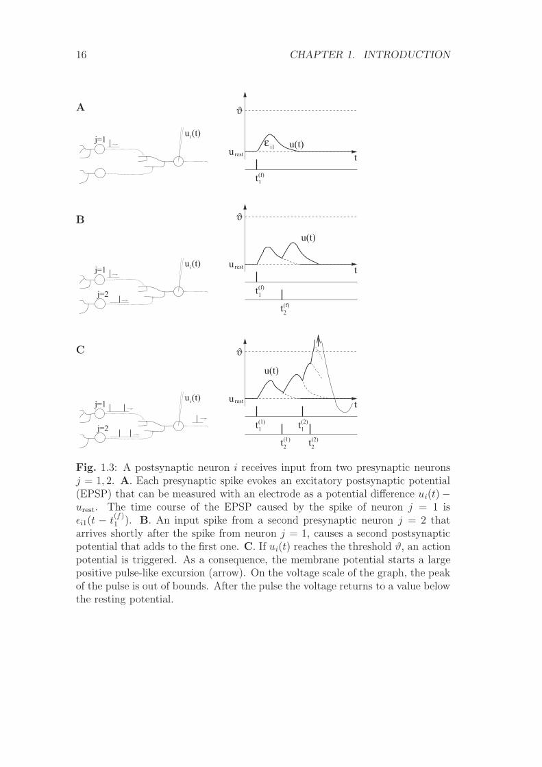
Fig. 1.3: A postsynaptic neuron i receives input from two presynaptic neuronsj = 1, 2. A. Each presynaptic spike evokes an excitatory postsynaptic potential(EPSP) that can be measured with an electrode as a potential difference ui(t)−urest. The time course of the EPSP caused by the spike of neuron j = 1 isεi1(t − t
(f)1 ). B. An input spike from a second presynaptic neuron j = 2 that
arrives shortly after the spike from neuron j = 1, causes a second postsynapticpotential that adds to the first one. C. If ui(t) reaches the threshold ϑ, an actionpotential is triggered. As a consequence, the membrane potential starts a largepositive pulse-like excursion (arrow). On the voltage scale of the graph, the peakof the pulse is out of bounds. After the pulse the voltage returns to a value belowthe resting potential.
1.3. A PHENOMENOLOGICAL NEURON MODEL 17
from below we say that neuron i fires a spike. The moment of threshold crossingdefines the firing time t
(f)i . The model makes use of the fact that action potentials
always have roughly the same form. The trajectory of the membrane potentialduring a spike can hence be described by a certain standard time course denotedby η(t− t
(f)i ).
1.3.1 Definition of the Model SRM0
Putting all elements together we have the following description of neuronal dy-namics. The variable ui describes the momentary value of the membrane potentialof neuron i. It is given by
ui(t) = η(t− ti) +∑
j
∑f
εij(t− t(f)j ) + urest (1.3)
where ti is the last firing time of neuron i, i.e., ti = max{t(f)i | t(f)
i < t}. Firingoccurs whenever ui reaches the threshold ϑ from below,
ui(t) = ϑ andd
dtui(t) > 0 =⇒ t = t
(f)i (1.4)
The term εij in (1.3) describes the response of neuron i to spikes of a presynapticneuron j. The term η in (1.3) describes the form of the spike and the spike-afterpotential.
Note that we are only interested in the potential difference, viz., the distancefrom the resting potential. By an appropriate shift of the voltage scale, we canalways set urest = 0. The value of u(t) is then directly the distance from theresting potential. This is implicitly assumed in most neuron models discussed inthis book.
The model defined in equations (1.3) and (1.4) is called SRM0 where SRM isshort for Spike Response Model (Gerstner, 1995). The subscript zero is intendedto remind the reader that it is a particularly simple ‘zero order’ version of thefull model that will be introduced in Chapter 4. Phenomenological models ofspiking neurons similar to the models SRM0 have a long tradition in theoreticalneuroscience (Hill, 1936; Stein, 1965; Geisler and Goldberg, 1966; Weiss, 1966).Some important limitations of the model SRM0 are discussed below in Section1.3.2. Despite the limitations, we hope to be able to show in the course of thisbook that spiking neuron models such as the Spike Response Model are a usefulconceptual framework for the analysis of neuronal dynamics and neuronal coding.
18 CHAPTER 1. INTRODUCTION
t
ϑ
u
t
η
0
η0
-
i(1)
(t-t )
δ(t-t )i(1)
(1)i
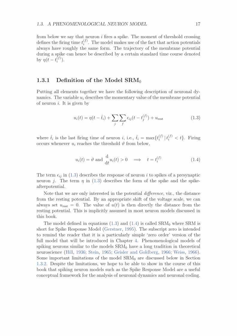
Fig. 1.4: In formal models of spiking neurons the shape of an action potential(dashed line) is usually replaced by a δ pulse (vertical line). The negative over-
shoot (spike-afterpotential) after the pulse is included in the kernel η(t − t(1)i )
(thick line) which takes care of ‘reset’ and ‘refractoriness’. The pulse is triggered
by the threshold crossing at t(1)i . Note that we have set urest = 0.
Example: Formal pulses
In a simple model, we may replace the exact form of the trajectory η during an ac-tion potential by, e.g., a square pulse, followed by a negative spike-afterpotential,
η(t− t(f)i ) =
⎧⎨⎩
1/Δt for 0 <t− t(f)i < Δt
−η0 exp
(− t−t
(f)i
τ
)for Δt < t− t
(f)i
(1.5)
with parameters η0, τ, Δt > 0. In the limit of Δt → 0 the square pulse approachesa Dirac δ function; see Fig. 1.4.
The positive pulse marks the moment of spike firing. For the purpose of themodel, it has no real significance, since the spikes are recorded explicitly in theset of firing times t
(1)i , t
(2)i , . . . . The negative spike-afterpotential, however, has
an important implication. It leads after the pulse to a ‘reset’ of the membranepotential to a value below threshold. The idea of a simple reset of the variable ui
after each spike is one of the essential components of the integrate-and-fire modelthat will be discussed in detail in Chapter 4.
If η0 � ϑ then the membrane potential after the pulse is significantly lowerthan the resting potential. The emission of a second pulse immediately after thefirst one is therefore more difficult, since many input spikes are needed to reachthe threshold. The negative spike-after potential in Eq. (1.5) is thus a simplemodel of neuronal refractoriness.
1.3. A PHENOMENOLOGICAL NEURON MODEL 19
Example: Formal spike trains
Throughout this book, we will refer to the moment when a given neuron emitsan action potential as the firing time of that neuron. In models, the firing timeis usually defined as the moment of threshold crossing. Similarly, in experimentsfiring times are recorded when the membrane potential reaches some thresholdvalue uϑ from below. We denote firing times of neuron i by t
(f)i where f = 1, 2, . . .
is the label of the spike. Formally, we may denote the spike train of a neuron ias the sequence of firing times
Si(t) =∑
f
δ(t− t(f)i ) (1.6)
where δ(x) us the Dirac δ function with δ(x) = 0 for x �= 0 and∫∞−∞ δ(x)dx = 1.
Spikes are thus reduced to points in time.
1.3.2 Limitations of the Model
The model presented in Section 1.3.1 is highly simplified and neglects many as-pects of neuronal dynamics. In particular, all postsynaptic potentials are assumedto have the same shape, independently of the state of the neuron. Furthermore,the dynamics of neuron i depends only on its most recent firing time ti. Let uslist the major limitations of this approach.
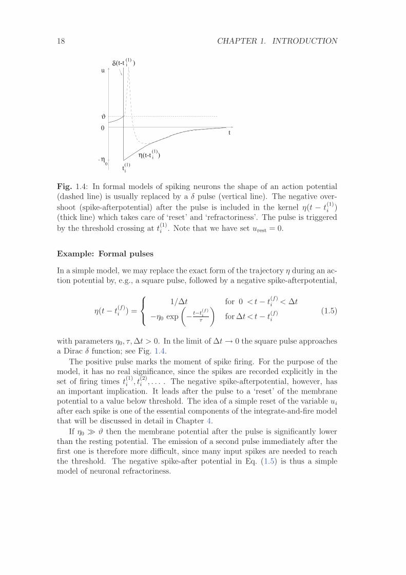
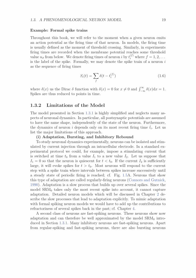
(i) Adaptation, Bursting, and Inhibitory ReboundTo study neuronal dynamics experimentally, neurons can be isolated and stim-
ulated by current injection through an intracellular electrode. In a standard ex-perimental protocol we could, for example, impose a stimulating current thatis switched at time t0 from a value I1 to a new value I2. Let us suppose thatI1 = 0 so that the neuron is quiescent for t < t0. If the current I2 is sufficientlylarge, it will evoke spikes for t > t0. Most neurons will respond to the currentstep with a spike train where intervals between spikes increase successively untila steady state of periodic firing is reached; cf. Fig. 1.5A. Neurons that showthis type of adaptation are called regularly-firing neurons (Connors and Gutnick,1990). Adaptation is a slow process that builds up over several spikes. Since themodel SRM0 takes only the most recent spike into account, it cannot captureadaptation. Detailed neuron models which will be discussed in Chapter 2 de-scribe the slow processes that lead to adaptation explicitly. To mimic adaptationwith formal spiking neuron models we would have to add up the contributions torefractoriness of several spikes back in the past; cf. Chapter 4.
A second class of neurons are fast-spiking neurons. These neurons show nowadaptation and can therefore be well approximated by the model SRM0 intro-duced in Section 1.3.1. Many inhibitory neurons are fast-spiking neurons. Apartfrom regular-spiking and fast-spiking neurons, there are also bursting neurons
20 CHAPTER 1. INTRODUCTION
A
B
C
D
0
0
0
0
2I
I2
I2
I1 t0
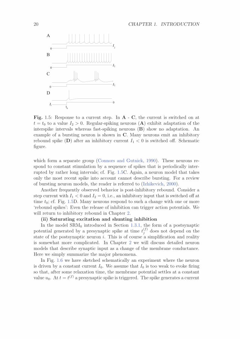
Fig. 1.5: Response to a current step. In A - C, the current is switched on att = t0 to a value I2 > 0. Regular-spiking neurons (A) exhibit adaptation of theinterspike intervals whereas fast-spiking neurons (B) show no adaptation. Anexample of a bursting neuron is shown in C. Many neurons emit an inhibitoryrebound spike (D) after an inhibitory current I1 < 0 is switched off. Schematicfigure.
which form a separate group (Connors and Gutnick, 1990). These neurons re-spond to constant stimulation by a sequence of spikes that is periodically inter-rupted by rather long intervals; cf. Fig. 1.5C. Again, a neuron model that takesonly the most recent spike into account cannot describe bursting. For a reviewof bursting neuron models, the reader is referred to (Izhikevich, 2000).
Another frequently observed behavior is post-inhibitory rebound. Consider astep current with I1 < 0 and I2 = 0, i.e., an inhibitory input that is switched off attime t0; cf. Fig. 1.5D. Many neurons respond to such a change with one or more‘rebound spikes’: Even the release of inhibition can trigger action potentials. Wewill return to inhibitory rebound in Chapter 2.
(ii) Saturating excitation and shunting inhibitionIn the model SRM0 introduced in Section 1.3.1, the form of a postsynaptic
potential generated by a presynaptic spike at time t(f)j does not depend on the
state of the postsynaptic neuron i. This is of course a simplification and realityis somewhat more complicated. In Chapter 2 we will discuss detailed neuronmodels that describe synaptic input as a change of the membrane conductance.Here we simply summarize the major phenomena.
In Fig. 1.6 we have sketched schematically an experiment where the neuronis driven by a constant current I0. We assume that I0 is too weak to evoke firingso that, after some relaxation time, the membrane potential settles at a constantvalue u0. At t = t(f) a presynaptic spike is triggered. The spike generates a current
1.3. A PHENOMENOLOGICAL NEURON MODEL 21
A Bu
urest
(f)t
u
urest
t (f)
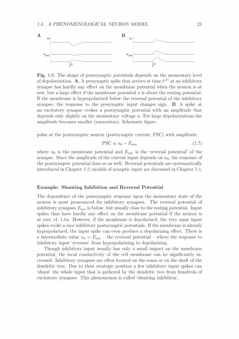
Fig. 1.6: The shape of postsynaptic potentials depends on the momentary levelof depolarization. A. A presynaptic spike that arrives at time t(f) at an inhibitorysynapse has hardly any effect on the membrane potential when the neuron is atrest, but a large effect if the membrane potential u is above the resting potential.If the membrane is hyperpolarized below the reversal potential of the inhibitorysynapse, the response to the presynaptic input changes sign. B. A spike atan excitatory synapse evokes a postsynaptic potential with an amplitude thatdepends only slightly on the momentary voltage u. For large depolarizations theamplitude becomes smaller (saturation). Schematic figure.
pulse at the postsynaptic neuron (postsynaptic current, PSC) with amplitude
PSC ∝ u0 − Esyn (1.7)
where u0 is the membrane potential and Esyn is the ‘reversal potential’ of thesynapse. Since the amplitude of the current input depends on u0, the response ofthe postsynaptic potential does so as well. Reversal potentials are systematicallyintroduced in Chapter 2.2; models of synaptic input are discussed in Chapter 2.4.
Example: Shunting Inhibition and Reversal Potential
The dependence of the postsynaptic response upon the momentary state of theneuron is most pronounced for inhibitory synapses. The reversal potential ofinhibitory synapses Esyn is below, but usually close to the resting potential. Inputspikes thus have hardly any effect on the membrane potential if the neuron isat rest; cf. 1.6a. However, if the membrane is depolarized, the very same inputspikes evoke a nice inhibitory postsynaptic potentials. If the membrane is alreadyhyperpolarized, the input spike can even produce a depolarizing effect. There isa intermediate value u0 = Esyn – the reversal potential – where the response toinhibitory input ‘reverses’ from hyperpolarizing to depolarizing.
Though inhibitory input usually has only a small impact on the membranepotential, the local conductivity of the cell membrane can be significantly in-creased. Inhibitory synapses are often located on the soma or on the shaft of thedendritic tree. Due to their strategic position a few inhibitory input spikes can‘shunt’ the whole input that is gathered by the dendritic tree from hundreds ofexcitatory synapses. This phenomenon is called ‘shunting inhibition’.
22 CHAPTER 1. INTRODUCTION
restu
t
i
i
ϑ
tt tj(f)j
(f)
u (t)
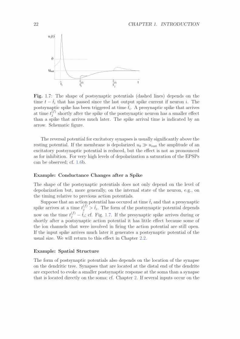
Fig. 1.7: The shape of postsynaptic potentials (dashed lines) depends on thetime t − ti that has passed since the last output spike current if neuron i. Thepostsynaptic spike has been triggered at time ti. A presynaptic spike that arrivesat time t
(f)j shortly after the spike of the postsynaptic neuron has a smaller effect
than a spike that arrives much later. The spike arrival time is indicated by anarrow. Schematic figure.
The reversal potential for excitatory synapses is usually significantly above theresting potential. If the membrane is depolarized u0 � urest the amplitude of anexcitatory postsynaptic potential is reduced, but the effect is not as pronouncedas for inhibition. For very high levels of depolarization a saturation of the EPSPscan be observed; cf. 1.6b.
Example: Conductance Changes after a Spike
The shape of the postsynaptic potentials does not only depend on the level ofdepolarization but, more generally, on the internal state of the neuron, e.g., onthe timing relative to previous action potentials.
Suppose that an action potential has occured at time ti and that a presynapticspike arrives at a time t
(f)j > ti. The form of the postsynaptic potential depends
now on the time t(f)j − ti; cf. Fig. 1.7. If the presynaptic spike arrives during or
shortly after a postsynaptic action potential it has little effect because some ofthe ion channels that were involved in firing the action potential are still open.If the input spike arrives much later it generates a postsynaptic potential of theusual size. We will return to this effect in Chapter 2.2.
Example: Spatial Structure
The form of postsynaptic potentials also depends on the location of the synapseon the dendritic tree. Synapses that are located at the distal end of the dendriteare expected to evoke a smaller postsynaptic response at the soma than a synapsethat is located directly on the soma; cf. Chapter 2. If several inputs occur on the
1.4. THE PROBLEM OF NEURONAL CODING 23
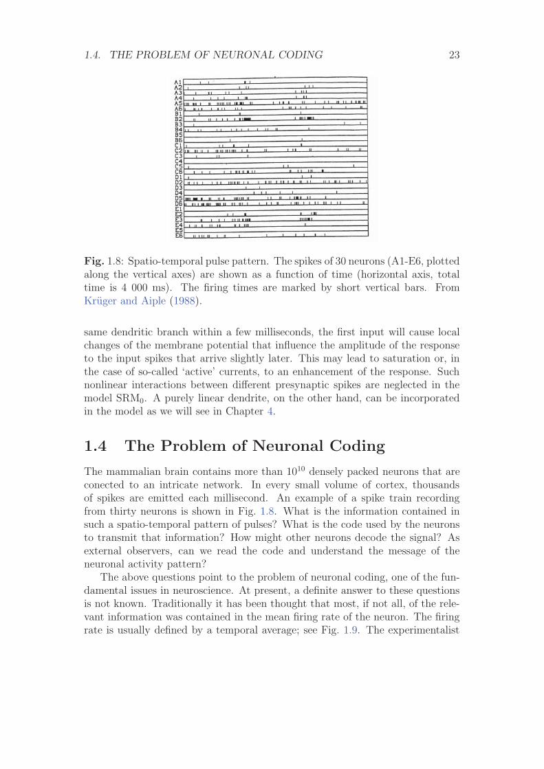
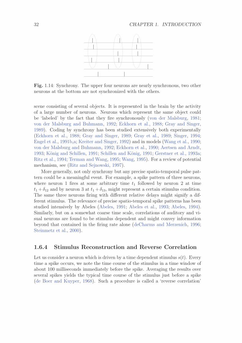
Fig. 1.8: Spatio-temporal pulse pattern. The spikes of 30 neurons (A1-E6, plottedalong the vertical axes) are shown as a function of time (horizontal axis, totaltime is 4 000 ms). The firing times are marked by short vertical bars. FromKruger and Aiple (1988).
same dendritic branch within a few milliseconds, the first input will cause localchanges of the membrane potential that influence the amplitude of the responseto the input spikes that arrive slightly later. This may lead to saturation or, inthe case of so-called ‘active’ currents, to an enhancement of the response. Suchnonlinear interactions between different presynaptic spikes are neglected in themodel SRM0. A purely linear dendrite, on the other hand, can be incorporatedin the model as we will see in Chapter 4.
1.4 The Problem of Neuronal Coding
The mammalian brain contains more than 1010 densely packed neurons that areconected to an intricate network. In every small volume of cortex, thousandsof spikes are emitted each millisecond. An example of a spike train recordingfrom thirty neurons is shown in Fig. 1.8. What is the information contained insuch a spatio-temporal pattern of pulses? What is the code used by the neuronsto transmit that information? How might other neurons decode the signal? Asexternal observers, can we read the code and understand the message of theneuronal activity pattern?
The above questions point to the problem of neuronal coding, one of the fun-damental issues in neuroscience. At present, a definite answer to these questionsis not known. Traditionally it has been thought that most, if not all, of the rele-vant information was contained in the mean firing rate of the neuron. The firingrate is usually defined by a temporal average; see Fig. 1.9. The experimentalist
24 CHAPTER 1. INTRODUCTION
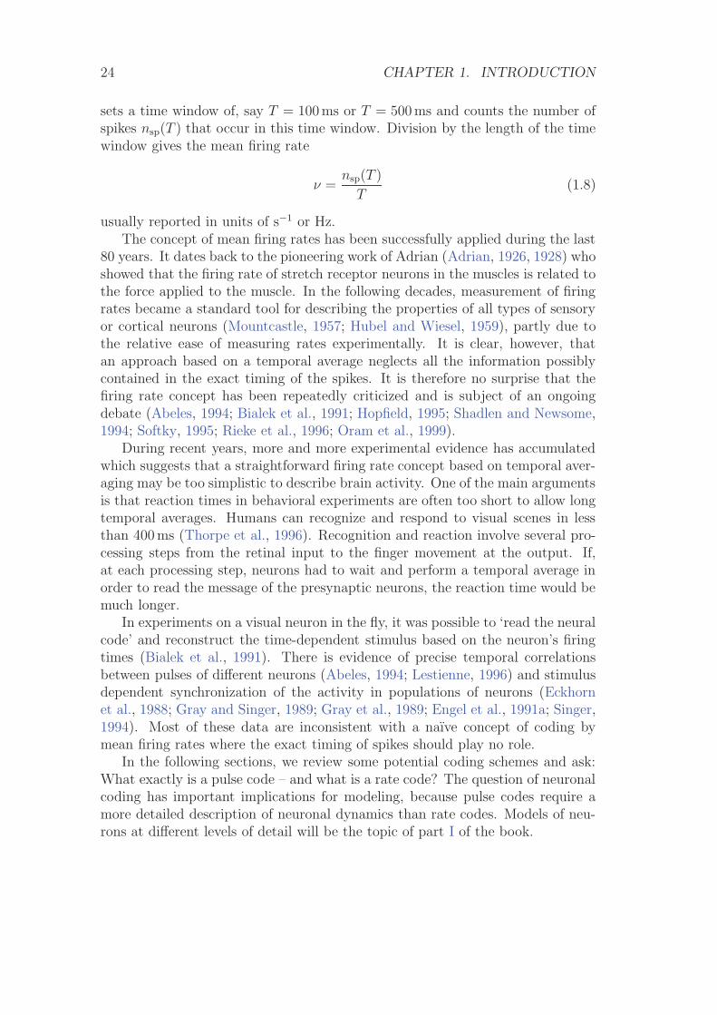
sets a time window of, say T = 100ms or T = 500ms and counts the number ofspikes nsp(T ) that occur in this time window. Division by the length of the timewindow gives the mean firing rate
ν =nsp(T )
T(1.8)
usually reported in units of s−1 or Hz.The concept of mean firing rates has been successfully applied during the last
80 years. It dates back to the pioneering work of Adrian (Adrian, 1926, 1928) whoshowed that the firing rate of stretch receptor neurons in the muscles is related tothe force applied to the muscle. In the following decades, measurement of firingrates became a standard tool for describing the properties of all types of sensoryor cortical neurons (Mountcastle, 1957; Hubel and Wiesel, 1959), partly due tothe relative ease of measuring rates experimentally. It is clear, however, thatan approach based on a temporal average neglects all the information possiblycontained in the exact timing of the spikes. It is therefore no surprise that thefiring rate concept has been repeatedly criticized and is subject of an ongoingdebate (Abeles, 1994; Bialek et al., 1991; Hopfield, 1995; Shadlen and Newsome,1994; Softky, 1995; Rieke et al., 1996; Oram et al., 1999).
During recent years, more and more experimental evidence has accumulatedwhich suggests that a straightforward firing rate concept based on temporal aver-aging may be too simplistic to describe brain activity. One of the main argumentsis that reaction times in behavioral experiments are often too short to allow longtemporal averages. Humans can recognize and respond to visual scenes in lessthan 400ms (Thorpe et al., 1996). Recognition and reaction involve several pro-cessing steps from the retinal input to the finger movement at the output. If,at each processing step, neurons had to wait and perform a temporal average inorder to read the message of the presynaptic neurons, the reaction time would bemuch longer.
In experiments on a visual neuron in the fly, it was possible to ‘read the neuralcode’ and reconstruct the time-dependent stimulus based on the neuron’s firingtimes (Bialek et al., 1991). There is evidence of precise temporal correlationsbetween pulses of different neurons (Abeles, 1994; Lestienne, 1996) and stimulusdependent synchronization of the activity in populations of neurons (Eckhornet al., 1988; Gray and Singer, 1989; Gray et al., 1989; Engel et al., 1991a; Singer,1994). Most of these data are inconsistent with a naıve concept of coding bymean firing rates where the exact timing of spikes should play no role.
In the following sections, we review some potential coding schemes and ask:What exactly is a pulse code – and what is a rate code? The question of neuronalcoding has important implications for modeling, because pulse codes require amore detailed description of neuronal dynamics than rate codes. Models of neu-rons at different levels of detail will be the topic of part I of the book.
1.5. RATE CODES 25
A B
t
nT
ν
spike count
= sp(single neuron, single run)
T
rate = average over time νmax
ν
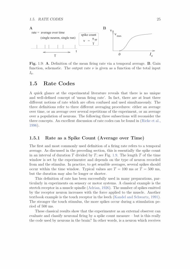
ϑ I0
Fig. 1.9: A. Definition of the mean firing rate via a temporal average. B. Gainfunction, schematic. The output rate ν is given as a function of the total inputI0.
1.5 Rate Codes
A quick glance at the experimental literature reveals that there is no uniqueand well-defined concept of ‘mean firing rate’. In fact, there are at least threedifferent notions of rate which are often confused and used simultaneously. Thethree definitions refer to three different averaging procedures: either an averageover time, or an average over several repetitions of the experiment, or an averageover a population of neurons. The following three subsections will reconsider thethree concepts. An excellent discussion of rate codes can be found in (Rieke et al.,1996).
1.5.1 Rate as a Spike Count (Average over Time)
The first and most commonly used definition of a firing rate refers to a temporalaverage. As discussed in the preceding section, this is essentially the spike countin an interval of duration T divided by T ; see Fig. 1.9. The length T of the timewindow is set by the experimenter and depends on the type of neuron recordedfrom and the stimulus. In practice, to get sensible averages, several spikes shouldoccur within the time window. Typical values are T = 100 ms or T = 500 ms,but the duration may also be longer or shorter.
This definition of rate has been successfully used in many preparations, par-ticularly in experiments on sensory or motor systems. A classical example is thestretch receptor in a muscle spindle (Adrian, 1926). The number of spikes emittedby the receptor neuron increases with the force applied to the muscle. Anothertextbook example is the touch receptor in the leech (Kandel and Schwartz, 1991).The stronger the touch stimulus, the more spikes occur during a stimulation pe-riod of 500 ms.
These classical results show that the experimenter as an external observer canevaluate and classify neuronal firing by a spike count measure – but is this reallythe code used by neurons in the brain? In other words, is a neuron which receives
26 CHAPTER 1. INTRODUCTION
signals from a sensory neuron only looking at and reacting to the number of spikesit receives in a time window of, say, 500 ms? We will approach this question froma modeling point of view later on in the book. Here we discuss some criticalexperimental evidence.
From behavioral experiments it is known that reaction times are often rathershort. A fly can react to new stimuli and change the direction of flight within30-40 ms; see the discussion in (Rieke et al., 1996). This is not long enoughfor counting spikes and averaging over some long time window. The fly has torespond after a postsynaptic neuron has received one or two spikes. Humans canrecognize visual scenes in just a few hundred milliseconds (Thorpe et al., 1996),even though recognition is believed to involve several processing steps. Again,this does not leave enough time to perform temporal averages on each level. Infact, humans can detect images in a sequence of unrelated pictures even if eachimage is shown for only 14 – 100 milliseconds (Keysers et al., 2001).
Temporal averaging can work well in cases where the stimulus is constantor slowly varying and does not require a fast reaction of the organism - andthis is the situation usually encountered in experimental protocols. Real-worldinput, however, is hardly stationary, but often changing on a fast time scale.For example, even when viewing a static image, humans perform saccades, rapidchanges of the direction of gaze. The image projected onto the retinal photoreceptors changes therefore every few hundred milliseconds.
Despite its shortcomings, the concept of a firing rate code is widely used notonly in experiments, but also in models of neural networks. It has led to the ideathat a neuron transforms information about a single input variable (the stimulusstrength) into a single continuous output variable (the firing rate); cf. Fig. 1.9B.The output rate ν increases with the stimulus strength and saturates for largeinput I0 towards a maximum value νmax. In experiments, a single neuron can bestimulated by injecting with an intra-cellular electrode a constant current I0. Therelation between the measured firing frequency ν and the applied input currentI0 is sometimes called the frequency-current curve of the neuron. In models, weformalize the relation between firing frequency (rate) and input current and writeν = g(I0). We refer to g as the neuronal gain function or transfer function.
From the point of view of rate coding, spikes are just a convenient way totransmit the analog output variable ν over long distances. In fact, the best codingscheme to transmit the value of the rate ν would be by a regular spike train withintervals 1/ν. In this case, the rate could be reliably measured after only twospikes. From the point of view of rate coding, the irregularities encountered inreal spike trains of neurons in the cortex must therefore be considered as noise.In order to get rid of the noise and arrive at a reliable estimate of the rate, theexperimenter (or the postsynaptic neuron) has to average over a larger numberof spikes. A critical discussion of the temporal averaging concept can be foundin (Shadlen and Newsome, 1994; Softky, 1995; Rieke et al., 1996).
1.5. RATE CODES 27
Δt1
tΔ
tΔ
(single neuron, repeated runs)
input
1st run
2nd
3rd...
ρ
spike density in PSTH
ρ =K1
tPSTH
rate = average over several runs
n (t; t+ )K
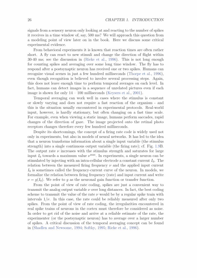
Fig. 1.10: Definition of the spike density in the Peri-Stimulus-Time Histogram(PSTH) as an average over several runs of the experiment.
1.5.2 Rate as a Spike Density (Average over Several Runs)
There is a second definition of rate which works for stationary as well as for time-dependent stimuli. The experimenter records from a neuron while stimulatingwith some input sequence. The same stimulation sequence is repeated severaltimes and the neuronal response is reported in a Peri-Stimulus-Time Histogram(PSTH); see Fig. 1.10. The time t is measured with respect to the start of thestimulation sequence and Δt is typically in the range of one or a few milliseconds.The number of occurrences of spikes nK(t; t + Δt) summed over all repetitionsof the experiment divided by the number K of repetitions is a measure of thetypical activity of the neuron between time t and t + Δt. A further division bythe interval length Δt yields the spike density of the PSTH
ρ(t) =1
Δt
nK(t; t + Δt)
K. (1.9)
Sometimes the result is smoothed to get a continuous ‘rate’ variable. The spikedensity of the PSTH is usually reported in units of Hz and often called the (time-dependent) firing rate of the neuron.
As an experimental procedure, the spike density measure is a useful methodto evaluate neuronal activity, in particular in the case of time-dependent stimuli.The obvious problem with this approach is that it can not be the decoding schemeused by neurons in the brain. Consider for example a frog which wants to catcha fly. It can not wait for the insect to fly repeatedly along exactly the sametrajectory. The frog has to base its decision on a single ‘run’ – each fly and eachtrajectory is different.
Nevertheless, the experimental spike density measure can make sense, if thereare large populations of independent neurons that receive the same stimulus.Instead of recording from a population of N neurons in a single run, it is ex-perimentally easier to record from a single neuron and average over N repeated
28 CHAPTER 1. INTRODUCTION
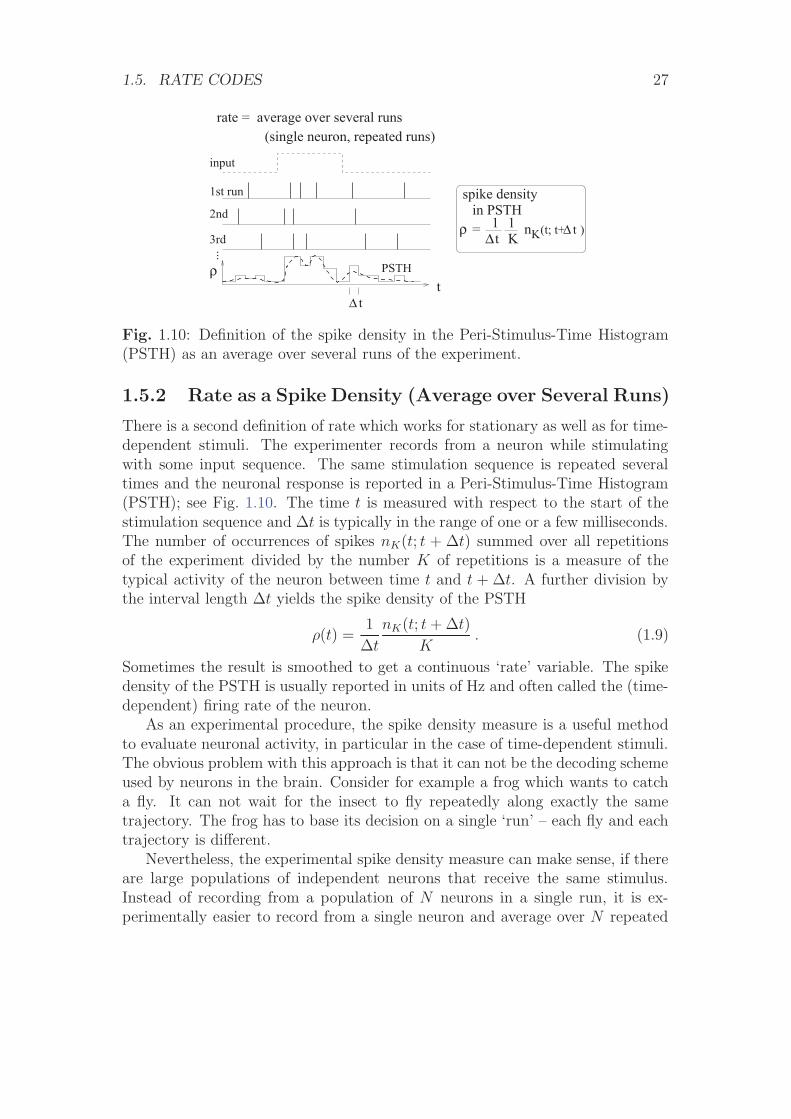
A B
populationpostsynapticneuron
AmΔt1A =
activity
Nn act (t;t+ t)Δ
(several neurons, single run)
j=1
3
N
2
...
Δt
rate = average over pool of equivalent neurons
Fig. 1.11: A. A postsynpatic neuron receives spike input from the population mwith activity Am. B. The population activity is defined as the fraction of neuronsthat are active in a short interval [t, t + Δt] divided by Δt.
runs. Thus, the spike density coding relies on the implicit assumption that thereare always populations of neurons and therefore leads us to the third notion of afiring rate, viz., a rate defined as a population average.
1.5.3 Rate as a Population Activity (Average over SeveralNeurons)
The number of neurons in the brain is huge. Often many neurons have similarproperties and respond to the same stimuli. For example, neurons in the pri-mary visual cortex of cats and monkeys are arranged in columns of cells withsimilar properties (Hubel and Wiesel, 1962, 1977; Hubel, 1988). Let us idealizethe situation and consider a population of neurons with identical properties. Inparticular, all neurons in the population should have the same pattern of inputand output connections. The spikes of the neurons in a population m are sentoff to another population n. In our idealized picture, each neuron in populationn receives input from all neurons in population m. The relevant quantity, fromthe point of view of the receiving neuron, is the proportion of active neurons inthe presynaptic population m; see Fig. 1.11A. Formally, we define the populationactivity
A(t) =1
Δt
nact(t; t + Δt)
N=
1
Δt
∫ t+Δt
t
∑j
∑f δ(t− t
(f)j ) dt
N(1.10)
where N is the size of the population, nact(t; t+Δt) the number of spikes (summedover all neurons in the population) that occur between t and t + Δt and Δt asmall time interval; see Fig. 1.11. Eq. (1.10) defines a variable with units s−1 –in other words, a rate.
The population activity may vary rapidly and can reflect changes in the stimu-lus conditions nearly instantaneously (Gerstner, 2000a; Brunel et al., 2001). Thus
1.6. SPIKE CODES 29
the population activity does not suffer from the disadvantages of a firing rate de-fined by temporal averaging at the single-unit level. A potential problem withthe definition (1.10) is that we have formally required a homogeneous populationof neurons with identical connections which is hardly realistic. Real populationswill always have a certain degree of heterogeneity both in their internal parame-ters and in their connectivity pattern. Nevertheless, rate as a population activity(of suitably defined pools of neurons) may be a useful coding principle in manyareas of the brain. For inhomogeneous populations, the definition (1.10) may bereplaced by a weighted average over the population.
Example: Population vector coding
We give an example of a weighted average in an inhomogeneous population. Letus suppose that we are studying a population of neurons which respond to astimulus x. We may think of x as the location of the stimulus in input space.Neuron i responds best to stimulus xi, another neuron j responds best to stimulusxj . In other words, we may say that the spikes for a neuron i ‘represent’ an inputvector xi and those of j an input vector xj . In a large population, many neuronswill be active simultaneously when a new stimulus x is represented. The locationof this stimulus can then be estimated from the weighted population average
xest(t) =
∫ t+Δt
t
∑j
∑f xj δ(t− t
(f)j ) dt∫ t+Δt
t
∑j
∑f δ(t− t
(f)j ) dt
(1.11)
Both numerator and denominator are closely related to the population activity(1.10). The estimate (1.11) has been successfully used for an interpretation ofneuronal activity in primate motor cortex (Georgopoulos et al., 1986; Wilson andMcNaughton, 1993). It is, however, not completely clear whether postsynapticneurons really evaluate the fraction (1.11). In any case, eq. (1.11) can be appliedby external observers to ‘decode’ neuronal signals, if the spike trains of a largenumber of neurons are accessible.
1.6 Spike Codes
In this section, we will briefly introduce some potential coding strategies basedon spike timing.
1.6.1 Time-to-First-Spike
Let us study a neuron which abruptly receives a ‘new’ input at time t0. Forexample, a neuron might be driven by an external stimulus which is suddenlyswitched on at time t0. This seems to be somewhat academic, but even in a
30 CHAPTER 1. INTRODUCTION
stimulus
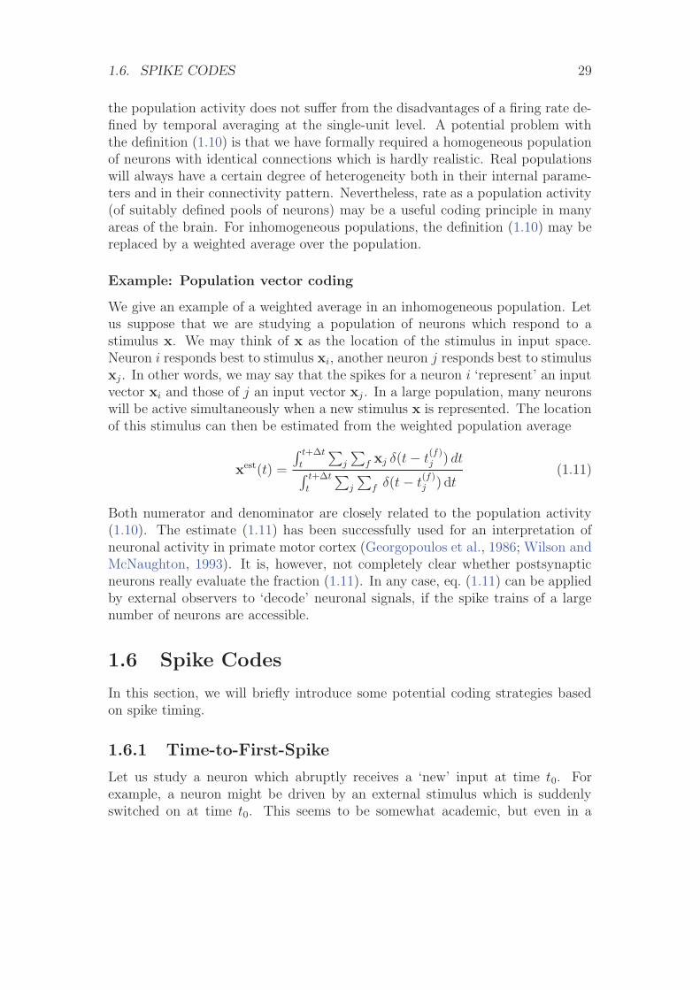
Fig. 1.12: Time-to-first spike. The spike train of three neurons are shown. Thethird neuron from the top is the first one to fire a spike after the stimulus onset(arrow). The dashed line indicates the time course of the stimulus.
realistic situation abrupt changes in the input are quite common. When we lookat a picture, our gaze jumps from one point to the next. After each saccade,the photo receptors in the retina receive a new visual input. Information aboutthe onset of a saccade would easily be available in the brain and could serve asan internal reference signal. We can then imagine a code where for each neuronthe timing of the first spike after the reference signal contains all informationabout the new stimulus. A neuron which fires shortly after the reference signalcould signal a strong stimulation, firing somewhat later would signal a weakerstimulation; see Fig. 1.12.
In a pure version of this coding scheme, each neuron only needs to fire a singlespike to transmit information. (If it emits several spikes, only the first spike afterthe reference signal counts. All following spikes would be irrelevant.) To imple-ment a clean version of such a coding scheme, we imagine that each neuron is shutoff by inhibition as soon as it has fired a spike. Inhibition ends with the onset ofthe next stimulus (e.g., after the next saccade). After the release from inhibitionthe neuron is ready to emit its next spike that now transmits information aboutthe new stimulus. Since each neuron in such a scenario transmits exactly onespike per stimulus, it is clear that only the timing conveys information and notthe number of spikes.
A coding scheme based on the time-to-first-spike is certainly an idealization.In a slightly different context coding by first spikes has been discussed by S.Thorpe (Thorpe et al., 1996). Thorpe argues that the brain does not have timeto evaluate more than one spike from each neuron per processing step. Thereforethe first spike should contain most of the relevant information. Using information-theoretic measures on their experimental data, several groups have shown thatmost of the information about a new stimulus is indeed conveyed during thefirst 20 or 50 milliseconds after the onset of the neuronal response (Optican andRichmond, 1987; Kjaer et al., 1994; Tovee et al., 1993; Tovee and Rolls, 1995).
1.6. SPIKE CODES 31
background oscillation
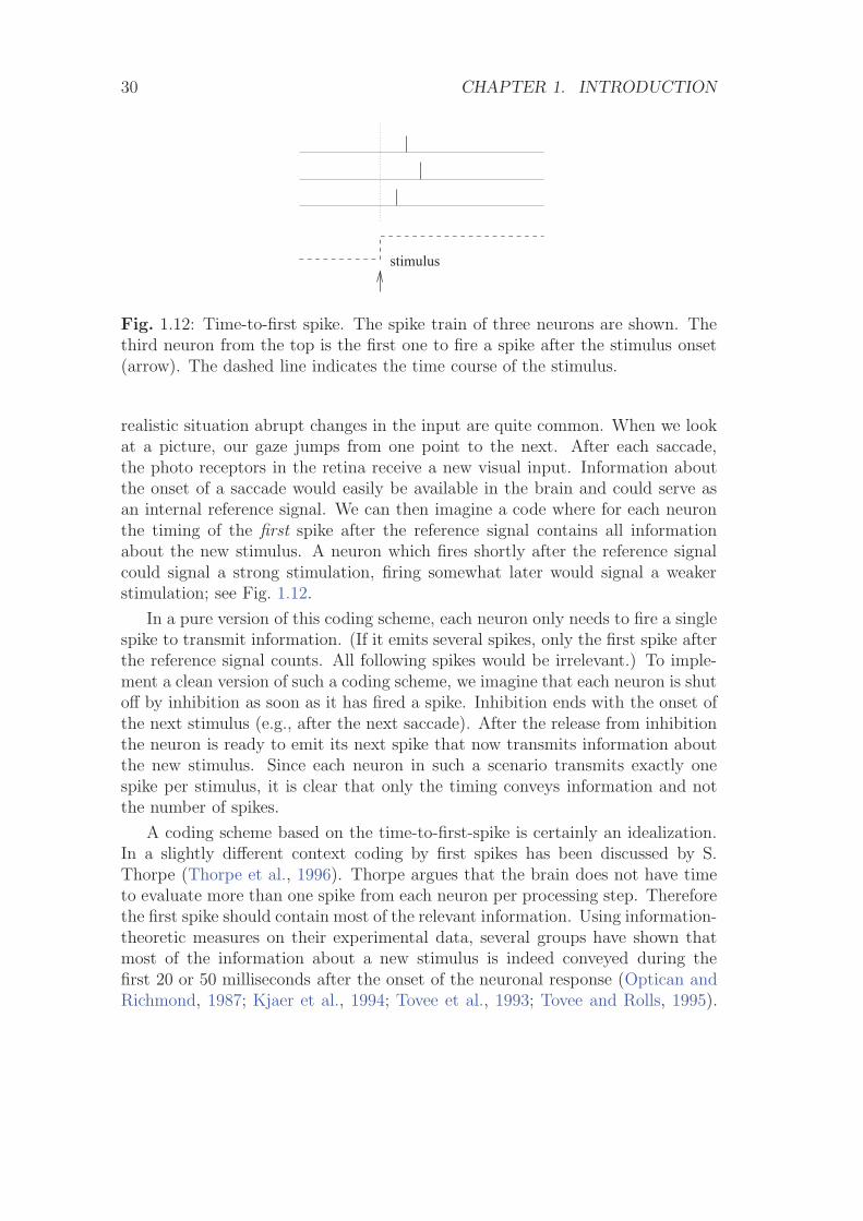
Fig. 1.13: Phase. The neurons fire at different phases with respect to the back-ground oscillation (dashed). The phase could code relevant information.
Rapid computation during the transients after a new stimulus has also beendiscussed in model studies (Hopfield and Herz, 1995; Tsodyks and Sejnowski,1995; van Vreeswijk and Sompolinsky, 1997; Treves et al., 1997). Since time-to-first spike is a highly simplified coding scheme, analytical studies are possible(Maass, 1998).
1.6.2 Phase
We can apply a code by ’time-to-first-spike’ also in the situation where the ref-erence signal is not a single event, but a periodic signal. In the hippocampus,in the olfactory system, and also in other areas of the brain, oscillations of someglobal variable (for example the population activity) are quite common. Theseoscillations could serve as an internal reference signal. Neuronal spike trains couldthen encode information in the phase of a pulse with respect to the backgroundoscillation. If the input does not change between one cycle and the next, thenthe same pattern of phases repeats periodically; see Fig. 1.13.
The concept of coding by phases has been studied by several different groups,not only in model studies (Hopfield, 1995; Jensen and Lisman, 1996; Maass, 1996),but also experimentally (O’Keefe, 1993). There is, for example, evidence thatthe phase of a spike during an oscillation in the hippocampus of the rat conveysinformation on the spatial location of the animal which is not fully accounted forby the firing rate of the neuron (O’Keefe, 1993).
1.6.3 Correlations and Synchrony
We can also use spikes from other neurons as the reference signal for a spike code.For example, synchrony between a pair or many neurons could signify specialevents and convey information which is not contained in the firing rate of theneurons; see Fig. 1.14. One famous idea is that synchrony could mean ‘belongingtogether’ (Milner, 1974; von der Malsburg, 1981). Consider for example a complex
32 CHAPTER 1. INTRODUCTION
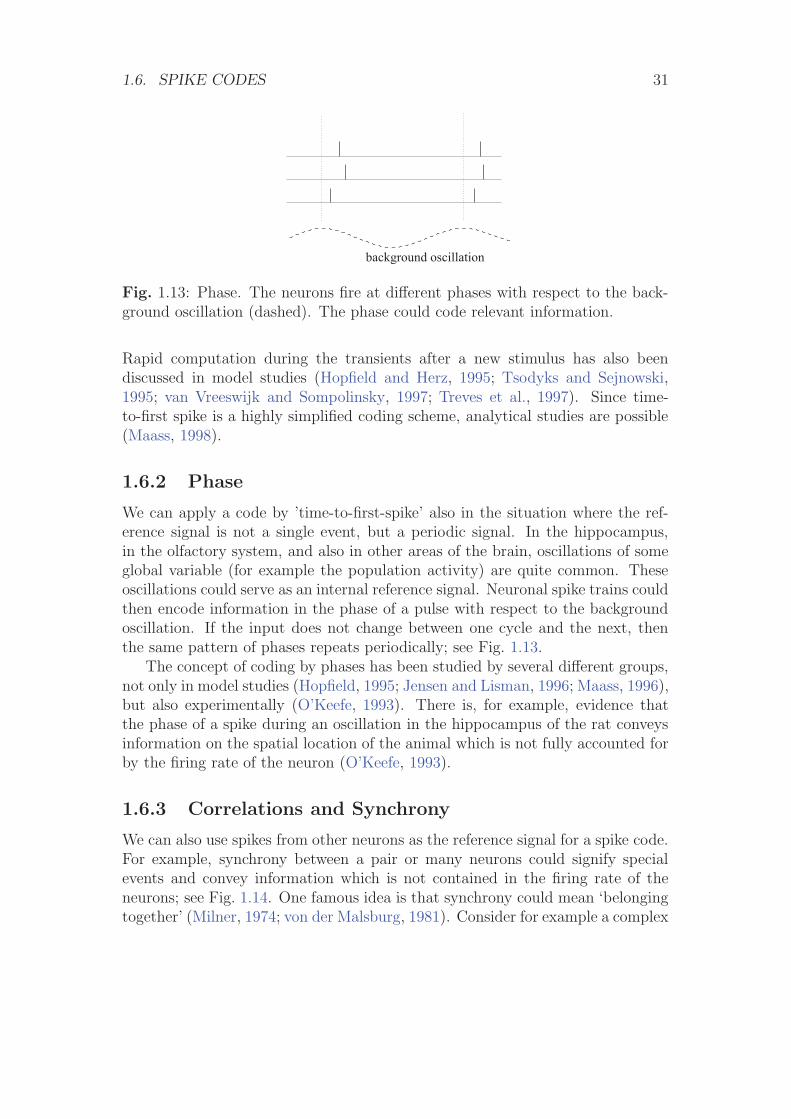
Fig. 1.14: Synchrony. The upper four neurons are nearly synchronous, two otherneurons at the bottom are not synchronized with the others.
scene consisting of several objects. It is represented in the brain by the activityof a large number of neurons. Neurons which represent the same object couldbe ‘labeled’ by the fact that they fire synchronously (von der Malsburg, 1981;von der Malsburg and Buhmann, 1992; Eckhorn et al., 1988; Gray and Singer,1989). Coding by synchrony has been studied extensively both experimentally(Eckhorn et al., 1988; Gray and Singer, 1989; Gray et al., 1989; Singer, 1994;Engel et al., 1991b,a; Kreiter and Singer, 1992) and in models (Wang et al., 1990;von der Malsburg and Buhmann, 1992; Eckhorn et al., 1990; Aertsen and Arndt,1993; Konig and Schillen, 1991; Schillen and Konig, 1991; Gerstner et al., 1993a;Ritz et al., 1994; Terman and Wang, 1995; Wang, 1995). For a review of potentialmechanism, see (Ritz and Sejnowski, 1997).
More generally, not only synchrony but any precise spatio-temporal pulse pat-tern could be a meaningful event. For example, a spike pattern of three neurons,where neuron 1 fires at some arbitrary time t1 followed by neuron 2 at timet1 + δ12 and by neuron 3 at t1 + δ13, might represent a certain stimulus condition.The same three neurons firing with different relative delays might signify a dif-ferent stimulus. The relevance of precise spatio-temporal spike patterns has beenstudied intensively by Abeles (Abeles, 1991; Abeles et al., 1993; Abeles, 1994).Similarly, but on a somewhat coarse time scale, correlations of auditory and vi-sual neurons are found to be stimulus dependent and might convey informationbeyond that contained in the firing rate alone (deCharms and Merzenich, 1996;Steinmetz et al., 2000).
1.6.4 Stimulus Reconstruction and Reverse Correlation
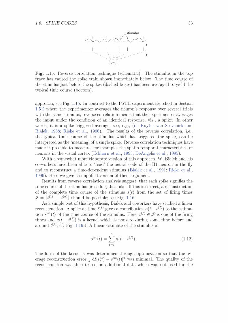
Let us consider a neuron which is driven by a time dependent stimulus s(t). Everytime a spike occurs, we note the time course of the stimulus in a time window ofabout 100 milliseconds immediately before the spike. Averaging the results overseveral spikes yields the typical time course of the stimulus just before a spike(de Boer and Kuyper, 1968). Such a procedure is called a ‘reverse correlation’
1.6. SPIKE CODES 33
t
t
stimulus
Fig. 1.15: Reverse correlation technique (schematic). The stimulus in the toptrace has caused the spike train shown immediately below. The time course ofthe stimulus just before the spikes (dashed boxes) has been averaged to yield thetypical time course (bottom).
approach; see Fig. 1.15. In contrast to the PSTH experiment sketched in Section1.5.2 where the experimenter averages the neuron’s response over several trialswith the same stimulus, reverse correlation means that the experimenter averagesthe input under the condition of an identical response, viz., a spike. In otherwords, it is a spike-triggered average; see, e.g., (de Ruyter van Stevenick andBialek, 1988; Rieke et al., 1996). The results of the reverse correlation, i.e.,the typical time course of the stimulus which has triggered the spike, can beinterpreted as the ‘meaning’ of a single spike. Reverse correlation techniques havemade it possible to measure, for example, the spatio-temporal characteristics ofneurons in the visual cortex (Eckhorn et al., 1993; DeAngelis et al., 1995).
With a somewhat more elaborate version of this approach, W. Bialek and hisco-workers have been able to ‘read’ the neural code of the H1 neuron in the flyand to reconstruct a time-dependent stimulus (Bialek et al., 1991; Rieke et al.,1996). Here we give a simplified version of their argument.
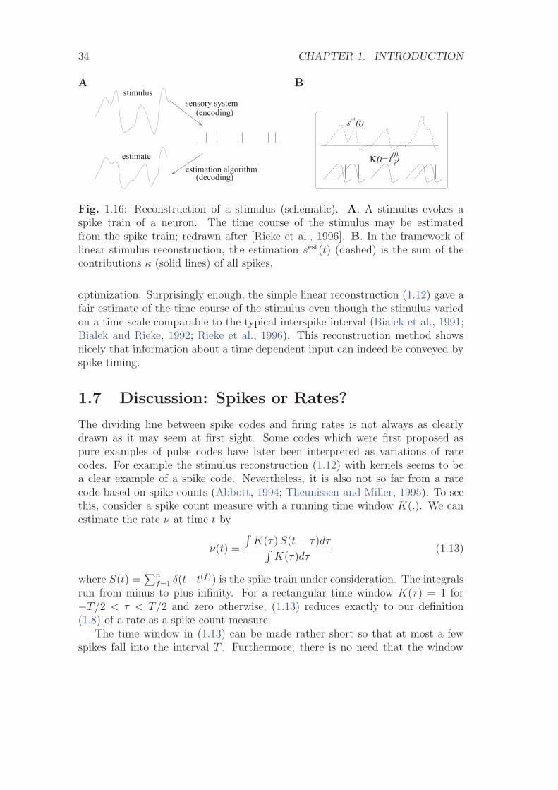
Results from reverse correlation analysis suggest, that each spike signifies thetime course of the stimulus preceding the spike. If this is correct, a reconstructionof the complete time course of the stimulus s(t) from the set of firing timesF = {t(1), . . . t(n)} should be possible; see Fig. 1.16.
As a simple test of this hypothesis, Bialek and coworkers have studied a linearreconstruction. A spike at time t(f) gives a contribution κ(t− t(f)) to the estima-tion sest(t) of the time course of the stimulus. Here, t(f) ∈ F is one of the firingtimes and κ(t − t(f)) is a kernel which is nonzero during some time before andaround t(f); cf. Fig. 1.16B. A linear estimate of the stimulus is
sest(t) =
n∑f=1
κ(t− t(f)) . (1.12)
The form of the kernel κ was determined through optimization so that the av-erage reconstruction error
∫dt[s(t) − sest(t)]2 was minimal. The quality of the
reconstruction was then tested on additional data which was not used for the
34 CHAPTER 1. INTRODUCTION
A Bstimulus
estimate
sensory system(encoding)
(decoding)estimation algorithm
(t−t )i(f)κ
est(t)s
Fig. 1.16: Reconstruction of a stimulus (schematic). A. A stimulus evokes aspike train of a neuron. The time course of the stimulus may be estimatedfrom the spike train; redrawn after [Rieke et al., 1996]. B. In the framework oflinear stimulus reconstruction, the estimation sest(t) (dashed) is the sum of thecontributions κ (solid lines) of all spikes.
optimization. Surprisingly enough, the simple linear reconstruction (1.12) gave afair estimate of the time course of the stimulus even though the stimulus variedon a time scale comparable to the typical interspike interval (Bialek et al., 1991;Bialek and Rieke, 1992; Rieke et al., 1996). This reconstruction method showsnicely that information about a time dependent input can indeed be conveyed byspike timing.
1.7 Discussion: Spikes or Rates?
The dividing line between spike codes and firing rates is not always as clearlydrawn as it may seem at first sight. Some codes which were first proposed aspure examples of pulse codes have later been interpreted as variations of ratecodes. For example the stimulus reconstruction (1.12) with kernels seems to bea clear example of a spike code. Nevertheless, it is also not so far from a ratecode based on spike counts (Abbott, 1994; Theunissen and Miller, 1995). To seethis, consider a spike count measure with a running time window K(.). We canestimate the rate ν at time t by
ν(t) =
∫K(τ) S(t− τ)dτ∫
K(τ)dτ(1.13)
where S(t) =∑n
f=1 δ(t−t(f)) is the spike train under consideration. The integralsrun from minus to plus infinity. For a rectangular time window K(τ) = 1 for−T/2 < τ < T/2 and zero otherwise, (1.13) reduces exactly to our definition(1.8) of a rate as a spike count measure.
The time window in (1.13) can be made rather short so that at most a fewspikes fall into the interval T . Furthermore, there is no need that the window
1.7. DISCUSSION: SPIKES OR RATES? 35
K(.) be symmetric and rectangular. We may just as well take an asymmetrictime window with smooth borders. Moreover, we can perform the integrationover the δ function which yields
ν(t) = cn∑
f=1
K(t− t(f)) (1.14)
where c = [∫
K(s)ds]−1 is a constant. Except for the constant c (which setsthe overall scale to units of one over time), the generalized rate formula (1.14)is now identical to the reconstruction formula (1.12). In other words, the linearreconstruction is just the firing rate measured with a cleverly optimized timewindow.
Similarly, a code based on the ’time-to-first-spike’ is also consistent with arate code. If, for example, the mean firing rate of a neuron is high for a givenstimulus, then the first spike is expected to occur early. If the rate is low, thefirst spike is expected to occur later. Thus the timing of the first spike containsa lot of information about the underlying rate.
Finally, a code based on population activities introduced above as an exampleof a rate code may be used for very fast temporal coding schemes. As discussedlater in Chapter 6, the population activity reacts quickly to any change in thestimulus. Thus rate coding in the sense of a population average is consistent withfast temporal information processing, whereas rate coding in the sense of a naıvespike count measure is not.
The discussion of whether or not to call a given code a rate code is stillongoing, even though precise definitions have been proposed (Theunissen andMiller, 1995). What is important, in our opinion, is to have a coding schemewhich allows neurons to quickly respond to stimulus changes. A naıve spikecount code with a long time window is unable to do this, but many of the othercodes are. The name of such a code, whether it is deemed a rate code or not isof minor importance.
Example: Towards a definition of rate codes
We have seen above in Eq. (1.14) that stimulus reconstruction with a linear kernelcan be seen as a special instance of a rate code. This suggests a formal definitionof a rate code via the reconstruction procedure: If all information contained in aspike train can be recovered by the linear reconstruction procedure of Eq. (1.12),then the neuron is, by definition, using a rate code. Spike codes would then becodes where a linear reconstruction is not successful. Theunissen and Miller haveproposed a definition of rate coding that makes the above ideas more precise(Theunissen and Miller, 1995).
To see how their definition works, we have to return to the reconstructionformula (1.12). It is, in fact, the first term of a systematic Volterra expansion for
36 CHAPTER 1. INTRODUCTION
the estimation of the stimulus from the spikes (Bialek et al., 1991)
sest(t) =∑
f
κ1(t− t(f)) +∑f,f ′
κ2(t− t(f), t− t(f′)) + . . . . (1.15)
For a specific neuron, inclusion of higher-order terms κ2, κ3, . . . may or may notimprove the quality of the estimation. For most neurons where the reconstructionhas been carried through it seems that the higher-order terms do not contributea large amount of information (Rieke et al., 1996). The neurons would then beclassified as rate coding.
Let us now suppose that the reconstruction procedure indicates a significantcontribution of the second-order term. Does this exclude rate coding? Unfortu-nately this is not the case. We have to exclude two other possibilities. Firstly, wemight have chosen a suboptimal stimulus. A neuron might for example encodethe variable x by a rate code, so that a nearly perfect linear reconstruction of xwould be possible,
x(t) ≈ xest =n∑
f=1
κ1;x(t− t(f)) ; (1.16)
But if we chose a stimulus s = x2 instead of x, then the reconstruction for sest
would involve second-order terms, even though the neuron is really using ratecode.
Secondly, according to Theunissen and Miller [1995] a spike code should showa temporal structure that is more precise than the temporal structure of thestimulus. The fact that neurons show precise and reliable spike timing as suchis, for them, not sufficient to classify the neuron as a temporal encoder, sincethe neuronal precision could just be the image of precise temporal input. Let usconsider a stimulus with cut-off frequency ω. In order to exclude the possibilitythat the timing is induced by the stimulus, Theunissen and Miller propose toconsider the Fourier spectrum of the higher-order reconstruction kernels. If theFourier transform of the higher-order kernels contains frequencies less than ω only,then the code is a rate code. If higher-order kernels are significant and containfrequencies above ω, then the information is encoded temporally. A positiveexample of a spike code (or of ‘temporal encoding’) according to this definitionwould be the code by correlation and synchrony introduced above. Anotherexample would be the phase code, in particular if the number of spikes per cycleis independent of the stimulus strength. For the exact mathematical definition ofa temporal code according to Theunissen and Miller, the reader is refered to theoriginal literature (Theunissen and Miller, 1995).
1.8. SUMMARY 37
1.8 Summary
The neuronal signal consists of short voltage pulses called action potentials orspikes. These pulses travel along the axon and are distributed to several post-synaptic neurons where they evoke postsynaptic potentials. If a postsynapticneuron receives several spikes from several presynaptic neurons within a shorttime window, its membrane potential may reach a critical value and an actionpotential is triggered. This action potential is the output signal which is, in turn,transmitted to other neurons.
The sequence of action potentials contains the information that is conveyedfrom one neuron to the next – but what is the code used by the neurons? Eventhough it is a question of fundamental importance the problem of neuronal cod-ing is still not fully resolved. We have reviewed three concepts of rate codes, viz.spike count over some time window, spike density in a histogram, and populationactivity in an ensemble of neurons. All three concepts have been successfully usedin experimental data analysis. All of these concepts are, however, problematicwhen they are interpreted as the actual code used for neuronal information trans-mission. A constructive criticism of rate codes may come from a presentation ofpotential spike codes, if their usefulness in terms of computational power or easeof implementation in biological hardware can be shown. It should be clear thatmodeling cannot give definite answers to the problem of neuronal coding. Thefinal answers have to come from experiments. One task of modeling may be todiscuss possible coding schemes, study their computational potential, exemplifytheir utility, and point out their limitations.
It is difficult to draw a clear border line between pulse and rate codes. What-ever the name of the code, it should offer a neural system the possibility to reactquickly to changes in the input. This seems to be a minimum requirement if fastbehavioral reaction times are to be accounted for.
If pulse coding is relevant, a description of information processing in the brainmust be based on spiking neuron models. If all information is contained in themean firing rate, then models on the level of rates suffice. Since we do not wantto take any decision a priori about the neuronal code, we concentrate in this bookon models of spiking neurons. In some cases, for example for stationary input,it will turn out that the spiking neuron models can be strictly reduced to ratemodels; in other cases such a reduction is not possible. By modeling on the levelof spiking neurons, the question of neuronal coding can thus be kept open.
Literature
An elementary, non-technical introduction to neurons and synapses can be foundin the book by Thompson (1993). At an intermediate level is “From neuron tobrain” by Kuffler et al. (1984). A standard textbook on Neuroscience covering a
38 CHAPTER 1. INTRODUCTION
wealth of experimental results is “Principles of Neural Science” by Kandel andSchwartz (1991).
Phenomenological spiking neuron models similar to the model discussed inSection 1.3.1 have a long tradition in theoretical neuroscience, e.g., (Lapicque,1907; Hill, 1936; McCulloch and Pitts, 1943; Stein, 1965; Geisler and Goldberg,1966; Weiss, 1966; Stein, 1967b). They are reviewed in Holden (1976), Tuckwell(1988), and Maass and Bishop (1998).
An excellent discussion of the problem of neuronal coding can be found inthe book ‘SPIKES - Exploring the neural code’ by Rieke et al. (1996). Thedebate of spikes versus rates is also highlighted in several papers (Abeles, 1994;Abbott, 1994; Shadlen and Newsome, 1994; Softky, 1995; Maass and Bishop,1998; Theunissen and Miller, 1995).
Part I
Single Neuron Models
39

Chapter 2
Detailed Neuron Models
From a biophysical point of view, action potentials are the result of currentsthat pass through ion channels in the cell membrane. In an extensive seriesof experiments on the giant axon of the squid, Hodgkin and Huxley succeededto measure these currents and to describe their dynamics in terms of differentialequations. In Section 2.2, the Hodgkin-Huxley model is reviewed and its behaviorillustrated by several examples.
The Hodgkin-Huxley equations are the starting point for detailed neuron mod-els which account for numerous ion channels, different types of synapse, and thespecific spatial geometry of an individual neuron. Ion channels, synaptic dynam-ics, and the spatial structure of dendrites are the topics of Sections 2.3–2.5. TheHodgkin-Huxley model is also an important reference model for the derivationof simplified neuron models in Chapters 3 and 4. Before we can turn to theHodgkin-Huxley equations, we need to give some additional information on theequilibrium potential of ion channels.
2.1 Equilibrium potential
Neurons are just as other cells enclosed by a membrane which separates the inte-rior of the cell from the extracellular space. Inside the cell the concentration ofions is different from that in the surrounding liquid. The difference in concentra-tion generates an electrical potential which plays an important role in neuronaldynamics. In this section, we want to provide some background information andgive an intuitive explanation of the equilibrium potential.
2.1.1 Nernst potential
From the theory of thermodynamics, it is known that the probability that amolecule takes a state of energy E is proportional to the Boltzmann factor p(E) ∝exp(−E/kT ) where k is the Boltzmann constant and T the temperature. Let us
41
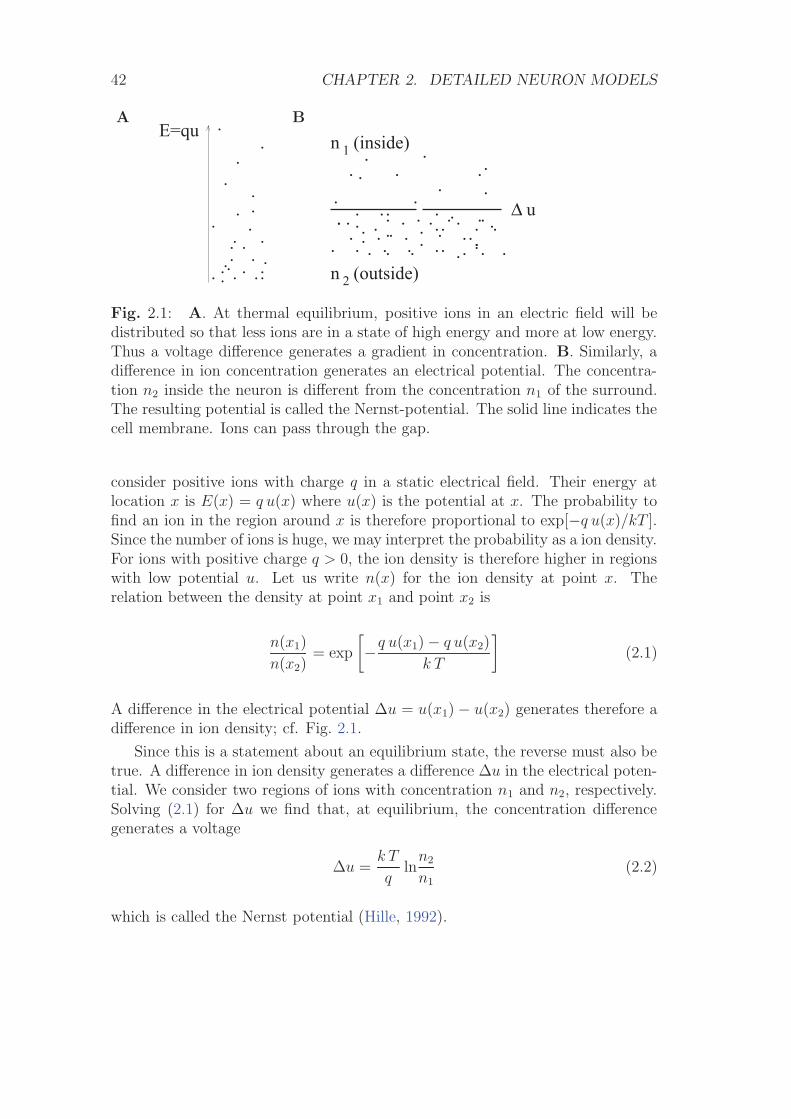
42 CHAPTER 2. DETAILED NEURON MODELS
A B
. . . .....
..
.
..
. ..
.
..
..
..
.
. .
Δ.
. ..
..
..
.. . . .. . .... . .
.
.. .. ... .
. . ..
. ..
. .... ..
.. .
...
. .... .. .
.
..
.
n (outside)
n (inside)
2
1E=qu
u
Fig. 2.1: A. At thermal equilibrium, positive ions in an electric field will bedistributed so that less ions are in a state of high energy and more at low energy.Thus a voltage difference generates a gradient in concentration. B. Similarly, adifference in ion concentration generates an electrical potential. The concentra-tion n2 inside the neuron is different from the concentration n1 of the surround.The resulting potential is called the Nernst-potential. The solid line indicates thecell membrane. Ions can pass through the gap.
consider positive ions with charge q in a static electrical field. Their energy atlocation x is E(x) = q u(x) where u(x) is the potential at x. The probability tofind an ion in the region around x is therefore proportional to exp[−q u(x)/kT ].Since the number of ions is huge, we may interpret the probability as a ion density.For ions with positive charge q > 0, the ion density is therefore higher in regionswith low potential u. Let us write n(x) for the ion density at point x. Therelation between the density at point x1 and point x2 is
n(x1)
n(x2)= exp
[−q u(x1)− q u(x2)
k T
](2.1)
A difference in the electrical potential Δu = u(x1)− u(x2) generates therefore adifference in ion density; cf. Fig. 2.1.
Since this is a statement about an equilibrium state, the reverse must also betrue. A difference in ion density generates a difference Δu in the electrical poten-tial. We consider two regions of ions with concentration n1 and n2, respectively.Solving (2.1) for Δu we find that, at equilibrium, the concentration differencegenerates a voltage
Δu =k T
qln
n2
n1(2.2)
which is called the Nernst potential (Hille, 1992).
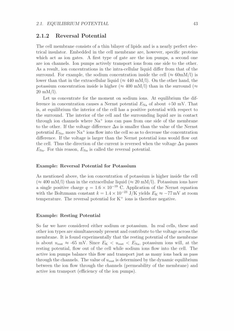
2.1. EQUILIBRIUM POTENTIAL 43
2.1.2 Reversal Potential
The cell membrane consists of a thin bilayer of lipids and is a nearly perfect elec-trical insulator. Embedded in the cell membrane are, however, specific proteinswhich act as ion gates. A first type of gate are the ion pumps, a second oneare ion channels. Ion pumps actively transport ions from one side to the other.As a result, ion concentrations in the intra-cellular liquid differ from that of thesurround. For example, the sodium concentration inside the cell (≈ 60mM/l) islower than that in the extracellular liquid (≈ 440 mM/l). On the other hand, thepotassium concentration inside is higher (≈ 400 mM/l) than in the surround (≈20 mM/l).
Let us concentrate for the moment on sodium ions. At equilibrium the dif-ference in concentration causes a Nernst potential ENa of about +50 mV. Thatis, at equilibrium the interior of the cell has a positive potential with respect tothe surround. The interior of the cell and the surrounding liquid are in contactthrough ion channels where Na+ ions can pass from one side of the membraneto the other. If the voltage difference Δu is smaller than the value of the Nernstpotential ENa, more Na+ ions flow into the cell so as to decrease the concentrationdifference. If the voltage is larger than the Nernst potential ions would flow outthe cell. Thus the direction of the current is reversed when the voltage Δu passesENa. For this reason, ENa is called the reversal potential.
Example: Reversal Potential for Potassium
As mentioned above, the ion concentration of potassium is higher inside the cell(≈ 400 mM/l) than in the extracellular liquid (≈ 20 mM/l). Potassium ions havea single positive charge q = 1.6 × 10⁻¹⁹ C. Application of the Nernst equationwith the Boltzmann constant k = 1.4× 10⁻²³ J/K yields EK ≈ −77mV at roomtemperature. The reversal potential for K+ ions is therefore negative.
Example: Resting Potential
So far we have considered either sodium or potassium. In real cells, these andother ion types are simultaneously present and contribute to the voltage across themembrane. It is found experimentally that the resting potential of the membraneis about urest ≈ -65 mV. Since EK < urest < ENa, potassium ions will, at theresting potential, flow out of the cell while sodium ions flow into the cell. Theactive ion pumps balance this flow and transport just as many ions back as passthrough the channels. The value of urest is determined by the dynamic equilibriumbetween the ion flow through the channels (permeability of the membrane) andactive ion transport (efficiency of the ion pumps).
44 CHAPTER 2. DETAILED NEURON MODELS
+
-
+ +
- -
+
-K
Naoutside
inside
K NaRC
I+
+
Fig. 2.2: Schematic diagram for the Hodgkin-Huxley model.
2.2 Hodgkin-Huxley Model
Hodgkin and Huxley (Hodgkin and Huxley, 1952) performed experiments on thegiant axon of the squid and found three different types of ion current, viz., sodium,potassium, and a leak current that consists mainly of Cl− ions. Specific voltage-dependent ion channels, one for sodium and another one for potassium, controlthe flow of those ions through the cell membrane. The leak current takes care ofother channel types which are not described explicitly.
2.2.1 Definition of the model
The Hodgkin-Huxley model can be understood with the help of Fig. 2.2. Thesemipermeable cell membrane separates the interior of the cell from the extracel-lular liquid and acts as a capacitor. If an input current I(t) is injected into thecell, it may add further charge on the capacitor, or leak through the channels inthe cell membrane. Because of active ion transport through the cell membrane,the ion concentration inside the cell is different from that in the extracellularliquid. The Nernst potential generated by the difference in ion concentration isrepresented by a battery.
Let us now translate the above considerations into mathematical equations.The conservation of electric charge on a piece of membrane implies that theapplied current I(t) may be split in a capacitive current IC which charges thecapacitor C and further components Ik which pass through the ion channels.Thus
I(t) = IC(t) +∑
k
Ik(t) (2.3)
where the sum runs over all ion channels. In the standard Hodgkin-Huxley modelthere are only three types of channel: a sodium channel with index Na, a potas-sium channel with index K and an unspecific leakage channel with resistance R;cf. Fig. 2.2. From the definition of a capacity C = Q/u where Q is a charge andu the voltage across the capacitor, we find the charging current IC = C du/dt.
Chapter 3
Two-Dimensional Neuron Models
The behavior of high-dimensional nonlinear differential equations is difficult tovisualize – and even more difficult to analyze. Two-dimensional differential equa-tions, however, can be studied in a transparent manner by means of a phase planeanalysis. A reduction of the four-dimensional equation of Hodgkin and Huxley toa two-variable neuron model is thus highly desirable. In the first section of thischapter we exploit the temporal properties of the gating variables of the Hodgkin-Huxley model so as to approximate the four-dimensional differential equation bya two-dimensional one. Section 3.2 is devoted to the phase plane analysis ofgeneric neuron models consisting of two coupled differential equations, one forthe membrane potential and the other one for the so-called relaxation variable.One of the questions to which we will return repeatedly throughout this chapteris the problem of the firing threshold. Section 3.3 summarizes some results onthreshold and excitability in two-dimensional models. As a first step, however,we have to go through the approximations that are necessary for a reduction ofthe Hodgkin-Huxley model to two dimensions.
3.1 Reduction to two dimensions
In this section we perform a systematic reduction of the four-dimensional Hodgkin-Huxley model to two dimensions. To do so, we have to eliminate two of the fourvariables. The essential ideas of the reduction can also be applied to detailedneuron models that may contain many different ion channels. In this case, morethan two variables would have to be eliminated, but the procedure would becompletely analogous (Kepler et al., 1992).
3.1.1 General approach
We focus on the Hodgkin-Huxley model discussed in Chapter 2.2 and start withtwo qualitative observations. First, we see from Fig. 2.3B that the time scale of
77
78 CHAPTER 3. TWO-DIMENSIONAL NEURON MODELS
the dynamics of the gating variable m is much faster than that of the variables n,h, and u. This suggests that we may treat m as an instantaneous variable. Thevariable m in the ion current equation (2.5) of the Hodgkin-Huxley model cantherefore be replaced by its steady-state value, m(t) → m0[u(t)]. This is what wecall a quasi steady state approximation.
Second, we see from Fig. 2.3B that the time constants τn(u) and τh(u) areroughly the same, whatever the voltage u. Moreover, the graphs of n0(u) and1−h0(u) in Fig. 2.3A are rather similar. This suggests that we may approximatethe two variables n and (1 − h) by a single effective variable w. To keep theformalism slightly more general we use a linear approximation (b−h) ≈ a n withsome constants a, b and set w = b − h = a n. With h = b − w, n = w/a, andm = m0(u), equations (2.4) - (2.5) become
Cdu
dt= −gNa[m0(u)]3 (b−w) (u−VNa)−gK
(w
a
)4
(u−VK)−gL (u−VL)+I , (3.1)
ordu
dt=
1
τ[F (u, w) + R I] , (3.2)
with R = g−1L , τ = R C and some function F . We now turn to the three equations
(2.6). The m equation has disappeared since m is treated as instantaneous.Instead of the two equations (2.6) for n and h, we are left with a single effectiveequation
dw
dt=
1
τwG(u, w) , (3.3)
where τw is a parameter and G a function that has to be specified. Eqs. (3.2) and(3.3) define a general two-dimensional neuron model. The mathematical details ofthe reduction of the four-dimensional Hodgkin-Huxley model to the two equations(3.2) and (3.3) are given below. Before we go through the mathematical step, wewill present two examples of two-dimensional neuron dynamics. We will returnto these examples repeatedly throughout this chapter.
Example: Morris-Lecar model
Morris and Lecar (1981) proposed a two-dimensional description of neuronal spikedynamics. A first equation describes the evolution of the membrane potential u,the second equation the evolution of a slow ‘recovery’ variable w. In dimensionlessvariables, the Morris-Lecar equations read
du
dt= −g1 m0(u) (u− 1)− g2 w (u− V2)− gL (u− VL) + I , (3.4)
dw
dt= − 1
τ(u)[w − w0(u)] . (3.5)
3.1. REDUCTION TO TWO DIMENSIONS 79
The voltage has been scaled so that one of the reversal potentials is unity. Timeis measured in units of τ = RC. If we compare Eq. (3.4) with Eq. (3.1), we notethat the first current term on the right-hand side of Eq. (3.1) has a factor (b−w)which closes the channel for high voltage and which is absent in (3.4). Anotherdifference is that neither m0 nor w in Eq. (3.4) have exponents. To clarify therelation between the two models, we could set m0(u) = [m0(u)]3 and w = (w/a)4.In the following we consider Eqs. (3.4) and (3.5) as a model in its own rights anddrop the hats over m0 and w.
The equilibrium functions shown in Fig. 2.3A typically have a sigmoidal shape.It is reasonable to approximate the voltage dependence by
m0(u) =1
2
[1 + tanh
(u− u1
u2
)](3.6)
w0(u) =1
2
[1 + tanh
(u− u3
u4
)](3.7)
with parameters u1, . . . , u4, and to approximate the time constant by
τ(u) =τw
cosh(
u−u3
u4
) (3.8)
with a further parameter τw.The Morris-Lecar model (3.4)–(3.8) gives a phenomenological description of
action potentials. Action potentials occur, if the current I is sufficiently strong.We will see later on that the firing threshold in the Morris-Lecar model can bediscussed by phase plane analysis.
Example: FitzHugh-Nagumo model
FitzHugh and Nagumo where probably the first to propose that, for a discussionof action potential generation, the four equations of Hodgkin and Huxley canbe replaced by two, i.e., Eqs. (3.2) and (3.3). They obtained sharp pulse-likeoscillations reminiscent of trains of action potentials by defining the functionsF (u, w) and G(u, w) as
F (u, w) = u− 1
3u3 − w
G(u, w) = b0 + b1 u− w , (3.9)
where u is the membrane voltage and w is a recovery variable (FitzHugh, 1961;Nagumo et al., 1962). Note that both F and G are linear in w; the sole non-linearity is the cubic term in u. The FitzHugh-Nagumo model is one of thesimplest model with non-trivial behavior lending itself to a phase plane analysis,which will be discussed below in Sections 3.2 and 3.3.
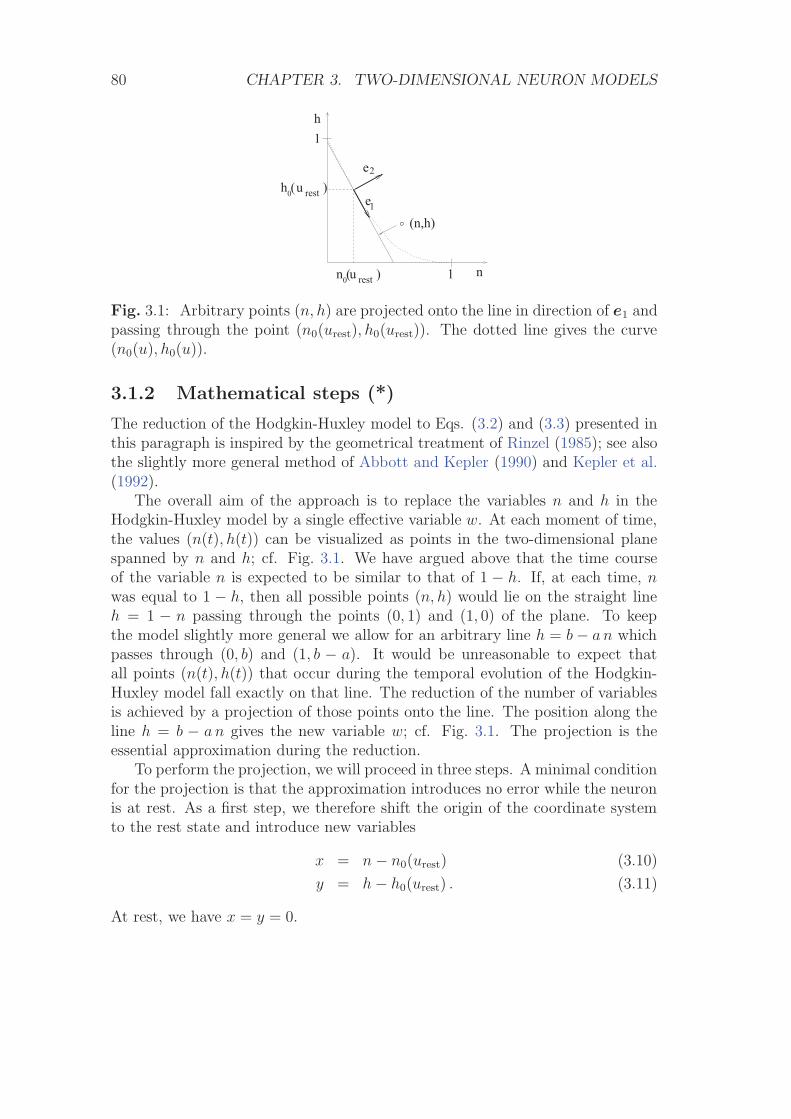
80 CHAPTER 3. TWO-DIMENSIONAL NEURON MODELS
restu
restu2
h
1
e1
e
n ( )
h ( )
0
0
n
(n,h)
1
Fig. 3.1: Arbitrary points (n, h) are projected onto the line in direction of e1 andpassing through the point (n0(urest), h0(urest)). The dotted line gives the curve(n0(u), h0(u)).
3.1.2 Mathematical steps (*)
The reduction of the Hodgkin-Huxley model to Eqs. (3.2) and (3.3) presented inthis paragraph is inspired by the geometrical treatment of Rinzel (1985); see alsothe slightly more general method of Abbott and Kepler (1990) and Kepler et al.(1992).
The overall aim of the approach is to replace the variables n and h in theHodgkin-Huxley model by a single effective variable w. At each moment of time,the values (n(t), h(t)) can be visualized as points in the two-dimensional planespanned by n and h; cf. Fig. 3.1. We have argued above that the time courseof the variable n is expected to be similar to that of 1 − h. If, at each time, nwas equal to 1 − h, then all possible points (n, h) would lie on the straight lineh = 1 − n passing through the points (0, 1) and (1, 0) of the plane. To keepthe model slightly more general we allow for an arbitrary line h = b− a n whichpasses through (0, b) and (1, b − a). It would be unreasonable to expect thatall points (n(t), h(t)) that occur during the temporal evolution of the Hodgkin-Huxley model fall exactly on that line. The reduction of the number of variablesis achieved by a projection of those points onto the line. The position along theline h = b − a n gives the new variable w; cf. Fig. 3.1. The projection is theessential approximation during the reduction.
To perform the projection, we will proceed in three steps. A minimal conditionfor the projection is that the approximation introduces no error while the neuronis at rest. As a first step, we therefore shift the origin of the coordinate systemto the rest state and introduce new variables
x = n− n0(urest) (3.10)
y = h− h0(urest) . (3.11)
At rest, we have x = y = 0.
3.1. REDUCTION TO TWO DIMENSIONS 81
Second, we turn the coordinate system by an angle α which is determined asfollows. For a given constant voltage u, the dynamics of the gating variables nand h approaches the equilibrium values (n0(u), h0(u)). The points (n0(u), h0(u))as a function of u define a curve in the two-dimensional plane. The slope of thecurve at u = urest yields the turning angle α via
tan α =dh0
du|urest
dn0
du|urest
. (3.12)
Turning the coordinate system by α moves the abscissa e1 of the new coordinatesystem in a direction tangential to the curve. The coordinates (z1, z2) in the newsystem are (
z1
z2
)=
(cos α sin α− sin α cos α
) (xy
). (3.13)
Third, we set z2 = 0 and retain only the coordinate z1 along e1. The inversetransform, (
xy
)=
(cos α − sin αsin α cos α
) (z1
z2
), (3.14)
yields x = z1 cos α and y = z1 sin α since z2 = 0. Hence, after the projection, thenew values of the variables n and h are
n′ = n0(urest) + z1 cos α , (3.15)
h′ = h0(urest) + z1 sin α . (3.16)
In principle, z1 can directly be used as the new effective variable. From (3.13)we find the differential equation
dz1
dt= cos α
dn
dt+ sin α
dh
dt. (3.17)
We use (2.7) and replace, on the right-hand side, n(t) and h(t) by (3.15) and(3.16). The result is
dz1
dt= − cos α
z1 cos α + n0(urest)− n0(u)
τn(u)− sin α
z1 sin α + h0(urest)− h0(u)
τh(u),
(3.18)which is of the form dz1/dt = G(u, z1), as desired.
To see the relation to Eqs. (3.1) and (3.3), it is convenient to rescale z1 anddefine
w = − tan α n0(urest)− z1 sin α . (3.19)
If we introduce a = − tan α, we find from Eq. (3.15) n′ = w/a and from Eq. (3.16)h′ = b− w which are the approximations that we have used in (3.1). The differ-ential equation for the variable w is of the desired form dw/dt = G(u, w) and can
82 CHAPTER 3. TWO-DIMENSIONAL NEURON MODELS
be found from Eq. (3.18). If we approximate the time constants τn and τh by acommon function τ(u), the dynamics of w is
dw
dt= − 1
τ(u)[w − w0(u)] . (3.20)
with a new equilibrium function w0(u) that is a linear combination of the functionsh0 and n0. From Eqs. (3.18) and (3.19) we find
w0(u) = − sin α [cosα n0(u) + sin α h0(u)− c] (3.21)
with a parameter c that is determined by direct calculation. In practice, bothw0(u) and τ(u) are fitted by the expressions (3.7) and (3.8).
3.2 Phase plane analysis
In two-dimensional models, the temporal evolution of the variables (u, w)T canbe visualized in the so-called phase plane. From a starting point (u(t), w(t))T thesystem will move in a time Δt to a new state (u(t + Δt), w(t + Δt))T which hasto be determined by integration of the differential equations (3.2) and (3.3). ForΔt sufficiently small, the displacement (Δu, Δw)T is in the direction of the flow(u, w)T , i.e., (
ΔuΔw
)=
(uw
)Δt , (3.22)
which can be plotted as a vector field in the phase plane. Here u = du/dt is givenby (3.2) and w = dw/dt by (3.3). The flow field is also called the phase portraitof the system. An important tool in the construction of the phase portrait arethe nullclines which are introduced now.
3.2.1 Nullclines
Let us consider the set of points with u = 0, called the u-nullcline. The directionof flow on the u-nullcline is in direction of (0, w)T , since u = 0. Hence arrowsin the phase portrait are vertical on the u-nullcline. Similarly, the w-nullcline isdefined by the condition w = 0 and arrows are horizontal. The fixed points of thedynamics, defined by u = w = 0 are given by the intersection of the u-nullclinewith the w-nullcline. In Fig. 3.2 we have three fixed points.
So far we have argued that arrows on the u-nullcline are vertical, but we do notknow yet whether they point up or down. To get the extra information needed,let us return to the w-nullcline. By definition, it separates the region with w > 0from the area with w < 0. Suppose we evaluate G(u, w) on the right-hand sideof Eq. (3.3) at a single point, e.g, at (0, 1). If G(0, 1) > 0, then the whole area
Chapter 4
Formal Spiking Neuron Models
Detailed conductance-based neuron models can reproduce electrophysiologicalmeasurements to a high degree of accuracy, but because of their intrinsic complex-ity these models are difficult to analyze. For this reason, simple phenomenologicalspiking neuron models are highly popular for studies of neural coding, memory,and network dynamics. In this chapter we discuss formal threshold models ofneuronal firing. Spikes are generated whenever the membrane potential u crossessome threshold ϑ from below. The moment of threshold crossing defines the firingtime t(f),
t(f) : u(t(f)) = ϑ anddu(t)
dt
∣∣∣∣t=t(f)
> 0 . (4.1)
Since spikes are stereotyped events they are fully characterized by their firingtime. We focus on models that are based on a single variable u. Some well-knowninstances of spiking neuron models differ in the specific way the dynamics of thevariable u is defined. We start our discussion with the integrate-and-fire neuron(Section 4.1) and turn then to the Spike Response Model (Section 4.2). In Sec-tion 4.3 we illustrate the relation of spiking neuron models to conductance-basedmodels. Section 4.4 outlines an analytical approach for a study of integrate-and-fire neurons with passive dendrites. As a first application of spiking neuronmodels we reconsider in Section 4.5 the problem of neuronal coding. The spik-ing neuron models introduced in this chapter form the basis for the analysis ofnetwork dynamics and learning in the following chapters.
4.1 Integrate-and-fire model
In this section, we give an overview of integrate-and-fire models. The leakyintegrate-and-fire neuron introduced in Section 4.1.1 is probably the best-knownexample of a formal spiking neuron model. Generalizations of the leaky integrate-and-fire model include the nonlinear integrate-and-fire model that is discussed in
101
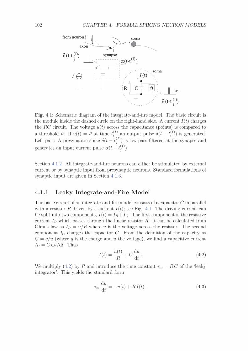
102 CHAPTER 4. FORMAL SPIKING NEURON MODELS
(f)(t-t )j
synapse
axon
from neuron j
I
R C ϑ
I
(f)(t-t )i
(t)
α
soma
soma
(f)j (t-t )
δ
δ
Fig. 4.1: Schematic diagram of the integrate-and-fire model. The basic circuit isthe module inside the dashed circle on the right-hand side. A current I(t) chargesthe RC circuit. The voltage u(t) across the capacitance (points) is compared to
a threshold ϑ. If u(t) = ϑ at time t(f)i an output pulse δ(t − t
(f)i ) is generated.
Left part: A presynaptic spike δ(t − t(f)j ) is low-pass filtered at the synapse and
generates an input current pulse α(t− t(f)j ).
Section 4.1.2. All integrate-and-fire neurons can either be stimulated by externalcurrent or by synaptic input from presynaptic neurons. Standard formulations ofsynaptic input are given in Section 4.1.3.
4.1.1 Leaky Integrate-and-Fire Model
The basic circuit of an integrate-and-fire model consists of a capacitor C in parallelwith a resistor R driven by a current I(t); see Fig. 4.1. The driving current canbe split into two components, I(t) = IR + IC. The first component is the resistivecurrent IR which passes through the linear resistor R. It can be calculated fromOhm’s law as IR = u/R where u is the voltage across the resistor. The secondcomponent IC charges the capacitor C. From the definition of the capacity asC = q/u (where q is the charge and u the voltage), we find a capacitive currentIC = C du/dt. Thus
I(t) =u(t)
R+ C
du
dt. (4.2)
We multiply (4.2) by R and introduce the time constant τm = R C of the ‘leakyintegrator’. This yields the standard form
τmdu
dt= −u(t) + R I(t) . (4.3)
4.1. INTEGRATE-AND-FIRE MODEL 103
We refer to u as the membrane potential and to τm as the membrane time constantof the neuron.
In integrate-and-fire models the form of an action potential is not describedexplicitly. Spikes are formal events characterized by a ‘firing time’ t(f). The firingtime t(f) is defined by a threshold criterion
t(f) : u(t(f)) = ϑ . (4.4)
Immediately after t(f), the potential is reset to a new value ur < ϑ,
limt→t(f);t>t(f)
u(t) = ur . (4.5)
For t > t(f) the dynamics is again given by (4.3) until the next threshold crossingoccurs. The combination of leaky integration (4.3) and reset (4.5) defines thebasic integrate-and-fire model (Stein, 1967b). We note that, since the membranepotential is never above threshold, the threshold condition (4.1) reduces to thecriterion (4.4), i.e., the condition on the slope du/dt can be dropped.
In its general version, the leaky integrate-and-fire neuron may also incorporatean absolute refractory period, in which case we proceed as follows. If u reachesthe threshold at time t = t(f), we interrupt the dynamics (4.3) during an absoluterefractory time Δabs and restart the integration at time t(f) + Δabs with the newinitial condition ur.
Example: Constant stimulation and firing rates
Before we continue with the definition of the integrate-and-fire model and itsvariants, let us study a simple example. Suppose that the integrate-and-fireneuron defined by (4.3)–(4.5) is stimulated by a constant input current I(t) = I0.For the sake of simplicity we take the reset potential to be ur = 0.
As a first step, let us calculate the time course of the membrane potential.We assume that a spike has occurred at t = t(1). The trajectory of the membranepotential can be found by integrating (4.3) with the initial condition u(t(1)) =ur = 0. The solution is
u(t) = R I0
[1− exp
(−t− t(1)
τm
)]. (4.6)
The membrane potential (4.6) approaches for t → ∞ the asymptotic valueu(∞) = R I0. For R I0 < ϑ no further spike can occur. For R I0 > ϑ, themembrane potential reaches the threshold ϑ at time t(2), which can be foundfrom the threshold condition u(t(2)) = ϑ or
ϑ = R I0
[1− exp
(−t(2) − t(1)
τm
)]. (4.7)
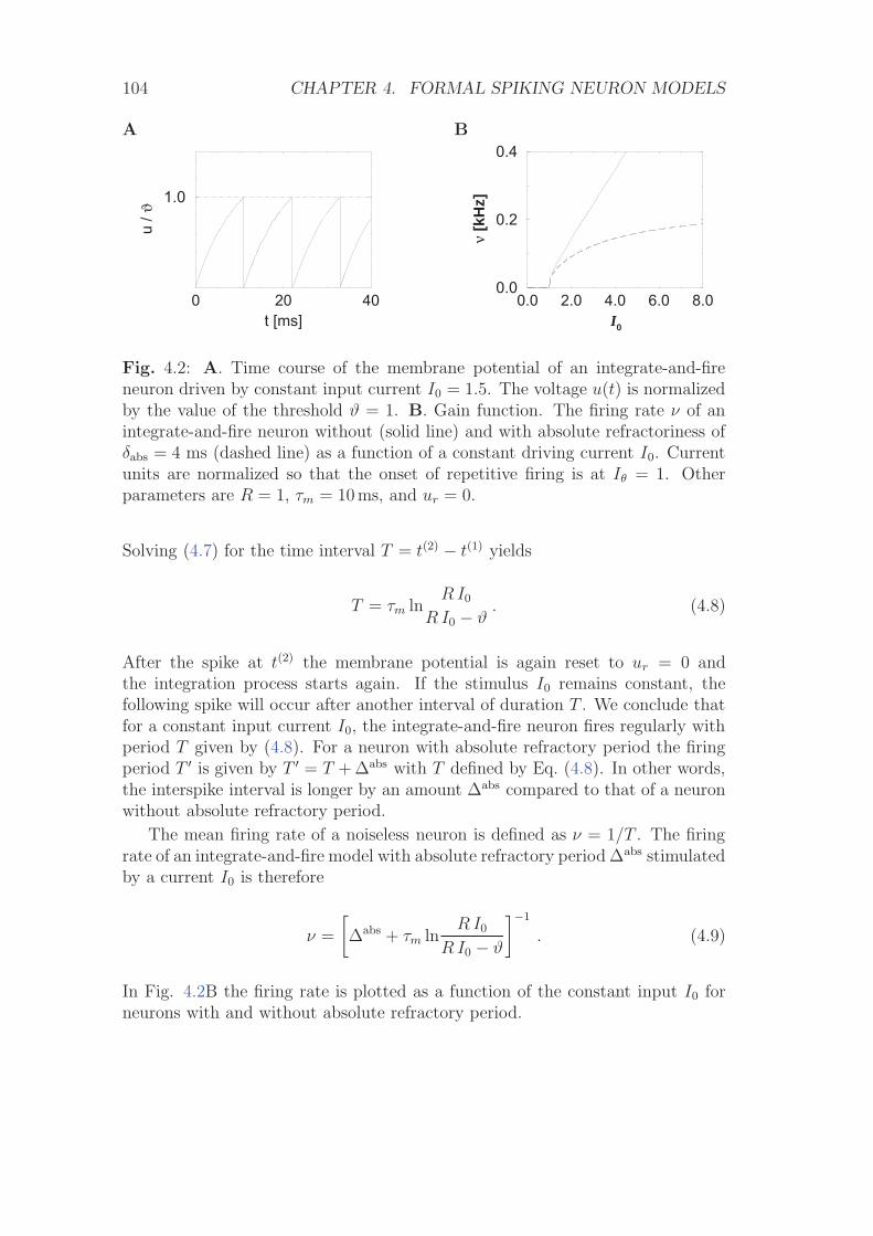
104 CHAPTER 4. FORMAL SPIKING NEURON MODELS
A
0 20 40t [ms]
1.0
u / ϑ
B
0.0 2.0 4.0 6.0 8.0 I0
0.0
0.2
0.4
ν [k
Hz]
Fig. 4.2: A. Time course of the membrane potential of an integrate-and-fireneuron driven by constant input current I0 = 1.5. The voltage u(t) is normalizedby the value of the threshold ϑ = 1. B. Gain function. The firing rate ν of anintegrate-and-fire neuron without (solid line) and with absolute refractoriness ofδabs = 4 ms (dashed line) as a function of a constant driving current I0. Currentunits are normalized so that the onset of repetitive firing is at Iθ = 1. Otherparameters are R = 1, τm = 10ms, and ur = 0.
Solving (4.7) for the time interval T = t(2) − t(1) yields
T = τm lnR I0
R I0 − ϑ. (4.8)
After the spike at t(2) the membrane potential is again reset to ur = 0 andthe integration process starts again. If the stimulus I0 remains constant, thefollowing spike will occur after another interval of duration T . We conclude thatfor a constant input current I0, the integrate-and-fire neuron fires regularly withperiod T given by (4.8). For a neuron with absolute refractory period the firingperiod T ′ is given by T ′ = T + Δabs with T defined by Eq. (4.8). In other words,the interspike interval is longer by an amount Δabs compared to that of a neuronwithout absolute refractory period.
The mean firing rate of a noiseless neuron is defined as ν = 1/T . The firingrate of an integrate-and-fire model with absolute refractory period Δabs stimulatedby a current I0 is therefore
ν =
[Δabs + τm ln
R I0
R I0 − ϑ
]−1
. (4.9)
In Fig. 4.2B the firing rate is plotted as a function of the constant input I0 forneurons with and without absolute refractory period.
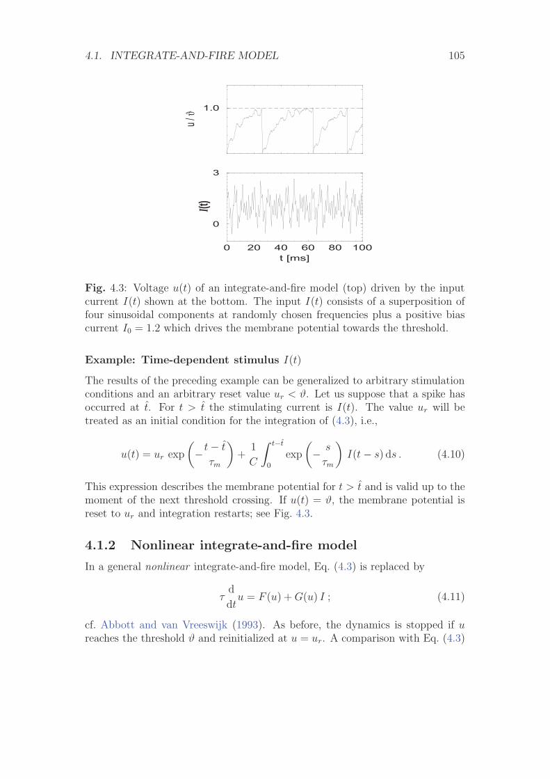
4.1. INTEGRATE-AND-FIRE MODEL 105
1.0
u / ϑ
0 20 40 60 80 100t [ms]
0
3
I(t)
Fig. 4.3: Voltage u(t) of an integrate-and-fire model (top) driven by the inputcurrent I(t) shown at the bottom. The input I(t) consists of a superposition offour sinusoidal components at randomly chosen frequencies plus a positive biascurrent I0 = 1.2 which drives the membrane potential towards the threshold.
Example: Time-dependent stimulus I(t)
The results of the preceding example can be generalized to arbitrary stimulationconditions and an arbitrary reset value ur < ϑ. Let us suppose that a spike hasoccurred at t. For t > t the stimulating current is I(t). The value ur will betreated as an initial condition for the integration of (4.3), i.e.,
u(t) = ur exp
(−t− t
τm
)+
1
C
∫ t−t
0
exp
(− s
τm
)I(t− s) ds . (4.10)
This expression describes the membrane potential for t > t and is valid up to themoment of the next threshold crossing. If u(t) = ϑ, the membrane potential isreset to ur and integration restarts; see Fig. 4.3.
4.1.2 Nonlinear integrate-and-fire model
In a general nonlinear integrate-and-fire model, Eq. (4.3) is replaced by
τd
dtu = F (u) + G(u) I ; (4.11)
cf. Abbott and van Vreeswijk (1993). As before, the dynamics is stopped if ureaches the threshold ϑ and reinitialized at u = ur. A comparison with Eq. (4.3)
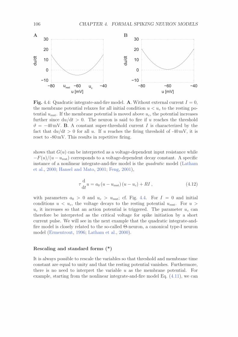
106 CHAPTER 4. FORMAL SPIKING NEURON MODELS
A
−80 −60 −40u [mV]
−10
0
10
20
30du
/dt
urest uc
B
−80 −60 −40u [mV]
−10
0
10
20
30
du/d
t
Fig. 4.4: Quadratic integrate-and-fire model. A. Without external current I = 0,the membrane potential relaxes for all initial condition u < uc to the resting po-tential urest. If the membrane potential is moved above uc, the potential increasesfurther since du/dt > 0. The neuron is said to fire if u reaches the thresholdϑ = −40mV. B. A constant super-threshold current I is characterized by thefact that du/dt > 0 for all u. If u reaches the firing threshold of -40mV, it isreset to -80mV. This results in repetitive firing.
shows that G(u) can be interpreted as a voltage-dependent input resistance while−F (u)/(u− urest) corresponds to a voltage-dependent decay constant. A specificinstance of a nonlinear integrate-and-fire model is the quadratic model (Lathamet al., 2000; Hansel and Mato, 2001; Feng, 2001),
τd
dtu = a0 (u− urest) (u− uc) + RI , (4.12)
with parameters a0 > 0 and uc > urest; cf. Fig. 4.4. For I = 0 and initialconditions u < uc, the voltage decays to the resting potential urest. For u >uc it increases so that an action potential is triggered. The parameter uc cantherefore be interpreted as the critical voltage for spike initiation by a shortcurrent pulse. We will see in the next example that the quadratic integrate-and-fire model is closely related to the so-called Θ-neuron, a canonical type-I neuronmodel (Ermentrout, 1996; Latham et al., 2000).
Rescaling and standard forms (*)
It is always possible to rescale the variables so that threshold and membrane timeconstant are equal to unity and that the resting potential vanishes. Furthermore,there is no need to interpret the variable u as the membrane potential. Forexample, starting from the nonlinear integrate-and-fire model Eq. (4.11), we can
4.1. INTEGRATE-AND-FIRE MODEL 107
introduce a new variable u by the transformation
u(t) −→ u(t) = τ
∫ u(t)
0
dx
G(x)(4.13)
which is possible if G(x) �= 0 for all x in the integration range. In terms of u wehave a new nonlinear integrate-and-fire model of the form
du
dt= γ(u) + I (t) (4.14)
with γ(u) = τF (u)/G(u). In other words, a general integrate-and-fire model(4.11) can always be reduced to the standard form (4.14). By a completely anal-ogous transformation, we could eliminate the function F in Eq. (4.11) and moveall the dependence into a new voltage dependent G (Abbott and van Vreeswijk,1993).
Example: Relation to a canonical type I model (*)
In this section, we show that there is a close relation between the quadraticintegrate-and-fire model (4.12) and the canonical type I phase model,
dφ
dt= [1− cos φ] + ΔI [1 + cos φ] ; (4.15)
cf. Section 3.2.4 (Ermentrout, 1996; Ermentrout and Kopell, 1986; Strogatz, 1994;Hoppensteadt and Izhikevich, 1997; Latham et al., 2000).
Let us denote by Iθ the minimal current necessary for repetitive firing of thequadratic integrate-and-fire neuron. With a suitable shift of the voltage scale andconstant current I = Iθ + ΔI the equation of the quadratic neuron model canthen be cast into the form
du
dt= u2 + ΔI . (4.16)
For ΔI > 0 the voltage increases until it reaches the firing threshold ϑ � 1where it is reset to a value ur −1. Note that the firing times are insensitiveto the actual values of firing threshold and reset value because the solution ofEq. (4.16) grows faster than exponentially and diverges for finite time (hyperbolicgrowth). The difference in the firing times for a finite threshold of, say, ϑ = 10and ϑ = 10 000 is thus negligible.
We want to show that the differential equation (4.16) can be transformed intothe canonical phase model (4.15) by the transformation
u(t) = tan
(φ(t)
2
). (4.17)
108 CHAPTER 4. FORMAL SPIKING NEURON MODELS
To do so, we take the derivative of (4.17) and use the differential equation (4.15)of the generic phase model. With help of the trigonometric relations d tanx/dx =1/ cos2(x) and 1 + cosx = cos2(x/2) we find
du
dt=
1
cos2(φ/2)
1
2
dφ
dt
= tan2(φ/2) + ΔI = u2 + ΔI . (4.18)
Thus Eq. (4.17) with φ(t) given by (4.15) is a solution to the differential equa-tion of the quadratic integrate-and-fire neuron. The quadratic integrate-and-fireneuron is therefore (in the limit ϑ→∞ and ur → −∞) equivalent to the generictype I neuron (4.15).
4.1.3 Stimulation by Synaptic Currents
So far we have considered an isolated neuron that is stimulated by an externalcurrent I(t). In a more realistic situation, the integrate-and-fire model is partof a larger network and the input current I(t) is generated by the activity ofpresynaptic neurons.
In the framework of the integrate-and-fire model, each presynaptic spike gen-erates a postsynaptic current pulse. More precisely, if the presynaptic neuron jhas fired a spike at t
(f)j , a postsynaptic neuron i ‘feels’ a current with time course
α(t− t(f)j ). The total input current to neuron i is the sum over all current pulses,
Ii(t) =∑
j
wij
∑f
α(t− t(f)j ) . (4.19)
The factor wij is a measure of the efficacy of the synapse from neuron j to neuroni.
Though Eq. (4.19) is a reasonable model of synaptic interaction, reality issomewhat more complicated, because the amplitude of the postsynaptic currentpulse depends on the actual value of the membrane potential ui. As we have seenin Chapter 2, each presynaptic action potential evokes a change in the conduc-tance of the postsynaptic membrane with a certain time course g(t − t(f)). The
postsynaptic current generated by a spike at time t(f)j is thus
α(t− t(f)j ) = −g(t− t
(f)j ) [ui(t)− Esyn] . (4.20)
The parameter Esyn is the reversal potential of the synapse.The level of the reversal potential depends on the type of synapse. For ex-
citatory synapses, Esyn is much larger than the resting potential. For a voltageui(t) close to the resting potential, we have ui(t) < Esyn. Hence the current Ii
induced by a presynaptic spike at an excitatory synapse is positive and increases
4.1. INTEGRATE-AND-FIRE MODEL 109
the membrane potential 1. The higher the voltage, the smaller the amplitude ofthe input current. Note that a positive voltage ui > urest is itself the result ofinput spikes which have arrived at other excitatory synapses. Hence, there is asaturation of the postsynaptic current and the total input current is not just thesum of independent contributions. Nevertheless, since the reversal potential ofexcitatory synapses is usually significantly above the firing threshold, the factor[ui − Esyn] is almost constant and saturation can be neglected.
For inhibitory synapses, the reversal potential is close to the resting poten-tial. An action potential arriving at an inhibitory synapse pulls the membranepotential towards the reversal potential Esyn. Thus, if the neuron is at rest, in-hibitory input hardly has any effect on the membrane potential. If the membranepotential is instead considerably above the resting potential, then the same inputhas a strong inhibitory effect. This is sometimes described as silent inhibition:inhibition is only seen if the membrane potential is above the resting potential.Strong silent inhibition is also called ‘shunting’ inhibition, because a significantlyreduced resistance of the membrane potential forms a short circuit that literallyshunts excitatory input the neuron might receive from other synapses.
Example: Pulse-coupling and α-function
The time course of the postsynaptic current α(s) introduced in Eq. (4.19) canbe defined in various ways. The simplest choice is a Dirac δ-pulse, α(s) = q δ(s),where q is the total charge that is injected in a postsynaptic neuron via a synapsewith efficacy wij = 1. More realistically, the postsynaptic current α should havea finite duration, e.g., as in the case of an exponential decay with time constantτs,
α(s) =q
τs
exp
(− s
τs
)Θ(s) . (4.21)
As usual, Θ is the Heaviside step function with Θ(s) = 1 for s > 0 and Θ(s) = 0else. Equation (4.21) is a simple way to account for the low-pass characteristicsof synaptic transmission; cf. Fig. 4.1.
An even more sophisticated version of α includes a finite rise time τr of thepostsynaptic current and a transmission delay Δax,
α(s) =q
τs − τr
[exp
(−s−Δax
τs
)− exp
(−s−Δax
τr
)]Θ(s−Δax) . (4.22)
In the limit of τr → τs, (4.22) yields
α(s) = qs−Δax
τ 2s
exp
(−s−Δax
τs
)Θ(s−Δax) . (4.23)
1Note that in Eq. (4.20) we consider the synaptic current as an external current whereasin Chapter 2 we have considered it as a membrane current and therefore used a different signconvention. In both cases, an excitatory input increases the membrane potential.
110 CHAPTER 4. FORMAL SPIKING NEURON MODELS
In the literature, a function of the form x exp(−x) such as (4.23) is often called anα-function. While this has motivated our choice of the symbol α for the synapticinput current, α may stand for any form of an input current pulse.
4.2 Spike response model (SRM)
The Spike Response Model (SRM) is – just like the nonlinear integrate-and-firemodel – a generalization of the leaky integrate-and-fire model. The direction ofthe generalization is, however, somewhat different. In the nonlinear integrate-and-fire model, parameters are made voltage dependent whereas in the SRMthey depend on the time since the last output spike. Another difference betweenintegrate-and-fire models and the SRM concerns the formulation of the equations.While integrate-and-fire models are usually defined in terms of differential equa-tions, the SRM expresses the membrane potential at time t as an integral overthe past.
The explicit dependence of the membrane potential upon the last output spikeallows us to model refractoriness as a combination of three components, viz., (i)a reduced responsiveness after an output spike; (ii) an increase in threshold afterfiring; and (iii) a hyperpolarizing spike after-potential. In Section 4.2.1 the SpikeResponse Model is introduced and its properties illustrated. Its relation to theintegrate-and-fire model is the topic of Section 4.2.2. An important special caseof the Spike Response Model is the simplified model SRM0 that we have alreadyencountered in Chapter 1.3.1. Section 4.2.3 will discuss it in more detail.
4.2.1 Definition of the SRM
In the framework of the Spike Response Model the state of a neuron i is describedby a single variable ui. In the absence of spikes, the variable ui is at its restingvalue, urest = 0. Each incoming spike will perturb ui and it takes some time beforeui returns to zero. The function ε describes the time course of the response to anincoming spike. If, after the summation of the effects of several incoming spikes,ui reaches the threshold ϑ an output spike is triggered. The form of the actionpotential and the after-potential is described by a function η. Let us supposeneuron i has fired its last spike at time ti. After firing the evolution of ui is givenby
ui(t) = η(t− ti) +∑
j
wij
∑f
εij(t− ti, t− t(f)j )
+
∫ ∞
0
κ(t− ti, s) Iext(t− s) ds (4.24)
4.2. SPIKE RESPONSE MODEL (SRM) 111
where t(f)j are spikes of presynaptic neurons j and wij is the synaptic efficacy. The
last term accounts for an external driving current I ext. The two sums run overall presynaptic neurons j and all firing times t
(f)j < t of neuron j. We emphasize
that all terms depend on t− ti, i.e., the time since the last output spike.In contrast to the integrate-and-fire neuron discussed in Section (4.1) the
threshold ϑ is not fixed but may also depend on t− ti
ϑ −→ ϑ(t− ti) . (4.25)
During an absolute refractory period Δabs, we may for example set ϑ to a largeand positive value to avoid firing and let it relax back to its equilibrium valuefor t > ti + Δabs. Firing occurs whenever the membrane potential ui reaches thedynamic threshold ϑ(t− ti) from below
t = t(f)i ⇔ ui(t) = ϑ(t− ti) and
dui(t)
dt> 0 . (4.26)
As mentioned before ti is the last firing time,
ti = max{t(f)i < t
}. (4.27)
Dynamic thresholds are a standard feature of phenomenological neuron models(Fuortes and Mantegazzini, 1962; Geisler and Goldberg, 1966; Weiss, 1966; Stein,1967b; MacGregor and Oliver, 1974; Horn and Usher, 1989; Eckhorn et al., 1990;Abeles, 1991). Models similar to Eqs. (4.24)–(4.26) can be traced back muchfurther; see, e.g., Hill (1936).
Interpretation
So far Eqs. (4.1) and (4.24) define a mathematical model. Can we give a biologicalinterpretation of the terms? Let us identify the variable ui with the membranepotential of neuron i. The functions η, κ and εij are response kernels that de-scribe the effect of spike emission and spike reception on the variable ui. Thisinterpretation has motivated the name ‘Spike Response Model’, SRM for short(Gerstner, 1995; Kistler et al., 1997). Let us discuss the meaning of the responsekernels.
The kernel η describes the standard form of an action potential of neuron iincluding the negative overshoot which typically follows a spike (after-potential).Graphically speaking, a contribution η is ‘pasted in’ each time the membranepotential reaches the threshold ϑ; cf. Fig. 4.5. Since the form of the spike is alwaysthe same, the exact time course of the action potential carries no information.What matters is whether there is the event ‘spike’ or not. The event is fullycharacterized by the firing time t
(f)i . In a simplified model, the form of the action
potential may therefore be neglected as long as we keep track of the firing times
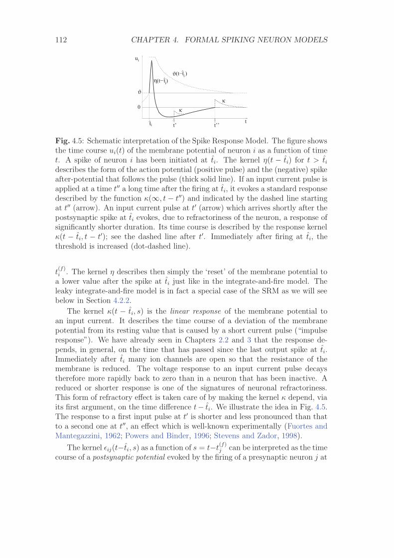
112 CHAPTER 4. FORMAL SPIKING NEURON MODELS
i(t− )ti(t− )
t
t
0
i
κ
κϑ
tt’ t’’
ui
ηϑ
Fig. 4.5: Schematic interpretation of the Spike Response Model. The figure showsthe time course ui(t) of the membrane potential of neuron i as a function of timet. A spike of neuron i has been initiated at ti. The kernel η(t − ti) for t > tidescribes the form of the action potential (positive pulse) and the (negative) spikeafter-potential that follows the pulse (thick solid line). If an input current pulse isapplied at a time t′′ a long time after the firing at ti, it evokes a standard responsedescribed by the function κ(∞, t− t′′) and indicated by the dashed line startingat t′′ (arrow). An input current pulse at t′ (arrow) which arrives shortly after thepostsynaptic spike at ti evokes, due to refractoriness of the neuron, a response ofsignificantly shorter duration. Its time course is described by the response kernelκ(t − ti, t − t′); see the dashed line after t′. Immediately after firing at ti, thethreshold is increased (dot-dashed line).
t(f)i . The kernel η describes then simply the ‘reset’ of the membrane potential to
a lower value after the spike at ti just like in the integrate-and-fire model. Theleaky integrate-and-fire model is in fact a special case of the SRM as we will seebelow in Section 4.2.2.
The kernel κ(t − ti, s) is the linear response of the membrane potential toan input current. It describes the time course of a deviation of the membranepotential from its resting value that is caused by a short current pulse (“impulseresponse”). We have already seen in Chapters 2.2 and 3 that the response de-pends, in general, on the time that has passed since the last output spike at ti.Immediately after ti many ion channels are open so that the resistance of themembrane is reduced. The voltage response to an input current pulse decaystherefore more rapidly back to zero than in a neuron that has been inactive. Areduced or shorter response is one of the signatures of neuronal refractoriness.This form of refractory effect is taken care of by making the kernel κ depend, viaits first argument, on the time difference t− ti. We illustrate the idea in Fig. 4.5.The response to a first input pulse at t′ is shorter and less pronounced than thatto a second one at t′′, an effect which is well-known experimentally (Fuortes andMantegazzini, 1962; Powers and Binder, 1996; Stevens and Zador, 1998).
The kernel εij(t−ti, s) as a function of s = t−t(f)j can be interpreted as the time
course of a postsynaptic potential evoked by the firing of a presynaptic neuron j at
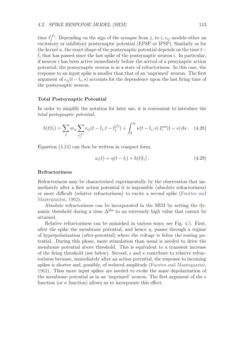
4.2. SPIKE RESPONSE MODEL (SRM) 113
time t(f)j . Depending on the sign of the synapse from j, to i, εij models either an
excitatory or inhibitory postsynaptic potential (EPSP or IPSP). Similarly as forthe kernel κ, the exact shape of the postsynaptic potential depends on the time t−ti that has passed since the last spike of the postsynaptic neuron i. In particular,if neuron i has been active immediately before the arrival of a presynaptic actionpotential, the postsynaptic neuron is in a state of refractoriness. In this case, theresponse to an input spike is smaller than that of an ‘unprimed’ neuron. The firstargument of εij(t− ti, s) accounts for the dependence upon the last firing time ofthe postsynaptic neuron.
Total Postsynaptic Potential
In order to simplify the notation for later use, it is convenient to introduce thetotal postsynaptic potential,
h(t|ti) =∑
j
wij
∑t(f)j
εij(t− ti, t− t(f)j ) +
∫ ∞
0
κ(t− ti, s) Iexti (t− s) ds . (4.28)
Equation (4.24) can then be written in compact form,
ui(t) = η(t− ti) + h(t|ti) . (4.29)
Refractoriness
Refractoriness may be characterized experimentally by the observation that im-mediately after a first action potential it is impossible (absolute refractoriness)or more difficult (relative refractoriness) to excite a second spike (Fuortes andMantegazzini, 1962).
Absolute refractoriness can be incorporated in the SRM by setting the dy-namic threshold during a time Δabs to an extremely high value that cannot beattained.
Relative refractoriness can be mimicked in various ways; see Fig. 4.5. First,after the spike the membrane potential, and hence η, passes through a regimeof hyperpolarization (after-potential) where the voltage is below the resting po-tential. During this phase, more stimulation than usual is needed to drive themembrane potential above threshold. This is equivalent to a transient increaseof the firing threshold (see below). Second, ε and κ contribute to relative refrac-toriness because, immediately after an action potential, the response to incomingspikes is shorter and, possibly, of reduced amplitude (Fuortes and Mantegazzini,1962). Thus more input spikes are needed to evoke the same depolarization ofthe membrane potential as in an ‘unprimed’ neuron. The first argument of the εfunction (or κ function) allows us to incorporate this effect.
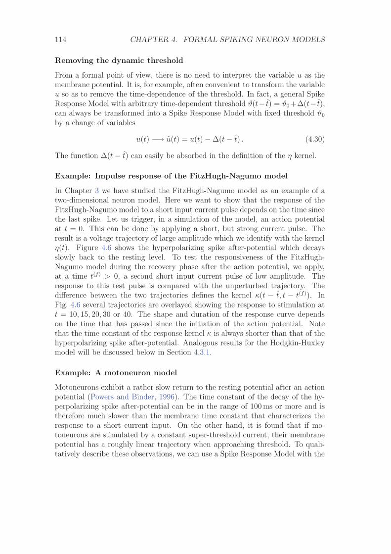
114 CHAPTER 4. FORMAL SPIKING NEURON MODELS
Removing the dynamic threshold
From a formal point of view, there is no need to interpret the variable u as themembrane potential. It is, for example, often convenient to transform the variableu so as to remove the time-dependence of the threshold. In fact, a general SpikeResponse Model with arbitrary time-dependent threshold ϑ(t− t) = ϑ0 +Δ(t− t),can always be transformed into a Spike Response Model with fixed threshold ϑ0
by a change of variables
u(t) −→ u(t) = u(t)−Δ(t− t) . (4.30)
The function Δ(t− t) can easily be absorbed in the definition of the η kernel.
Example: Impulse response of the FitzHugh-Nagumo model
In Chapter 3 we have studied the FitzHugh-Nagumo model as an example of atwo-dimensional neuron model. Here we want to show that the response of theFitzHugh-Nagumo model to a short input current pulse depends on the time sincethe last spike. Let us trigger, in a simulation of the model, an action potentialat t = 0. This can be done by applying a short, but strong current pulse. Theresult is a voltage trajectory of large amplitude which we identify with the kernelη(t). Figure 4.6 shows the hyperpolarizing spike after-potential which decaysslowly back to the resting level. To test the responsiveness of the FitzHugh-Nagumo model during the recovery phase after the action potential, we apply,at a time t(f) > 0, a second short input current pulse of low amplitude. Theresponse to this test pulse is compared with the unperturbed trajectory. Thedifference between the two trajectories defines the kernel κ(t − t, t − t(f)). InFig. 4.6 several trajectories are overlayed showing the response to stimulation att = 10, 15, 20, 30 or 40. The shape and duration of the response curve dependson the time that has passed since the initiation of the action potential. Notethat the time constant of the response kernel κ is always shorter than that of thehyperpolarizing spike after-potential. Analogous results for the Hodgkin-Huxleymodel will be discussed below in Section 4.3.1.
Example: A motoneuron model
Motoneurons exhibit a rather slow return to the resting potential after an actionpotential (Powers and Binder, 1996). The time constant of the decay of the hy-perpolarizing spike after-potential can be in the range of 100ms or more and istherefore much slower than the membrane time constant that characterizes theresponse to a short current input. On the other hand, it is found that if mo-toneurons are stimulated by a constant super-threshold current, their membranepotential has a roughly linear trajectory when approaching threshold. To quali-tatively describe these observations, we can use a Spike Response Model with the
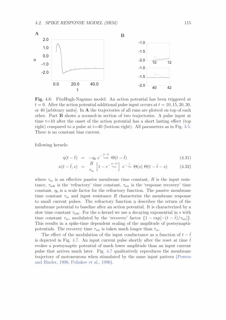
4.2. SPIKE RESPONSE MODEL (SRM) 115
A
0.0 20.0 40.0t
-2.0
-1.0
0.0
1.0
2.0u
B
10 12-2.0
-1.5
-1.0
40 42-2.0
-1.5
-1.0
Fig. 4.6: FitzHugh-Nagumo model. An action potential has been triggered att = 0. After the action potential additional pulse input occurs at t = 10, 15, 20, 30,or 40 [arbitrary units]. In A the trajectories of all runs are plotted on top of eachother. Part B shows a zoomed-in section of two trajectories. A pulse input attime t=10 after the onset of the action potential has a short lasting effect (topright) compared to a pulse at t=40 (bottom right). All parameters as in Fig. 3.5.There is no constant bias current.
following kernels:
η(t− t) = −η0 e− (t−t)
τrefr Θ(t− t) (4.31)
κ(t− t, s) =R
τm
[1− e−
(t−t)τrec
]e−
sτm Θ(s) Θ(t− t− s) (4.32)
where τm is an effective passive membrane time constant, R is the input resis-tance, τrefr is the ‘refractory’ time constant, τrec is the ‘response recovery’ timeconstant, η0 is a scale factor for the refractory function. The passive membranetime constant τm and input resistance R characterize the membrane responseto small current pulses. The refractory function η describes the return of themembrane potential to baseline after an action potential. It is characterized by aslow time constant τrefr. For the κ-kernel we use a decaying exponential in s withtime constant τm, modulated by the ‘recovery’ factor {1 − exp[−(t − t)/τrec]}.This results in a spike-time dependent scaling of the amplitude of postsynapticpotentials. The recovery time τrec is taken much longer than τm.
The effect of the modulation of the input conductance as a function of t − tis depicted in Fig. 4.7. An input current pulse shortly after the reset at time tevokes a postsynaptic potential of much lower amplitude than an input currentpulse that arrives much later. Fig. 4.7 qualitatively reproduces the membranetrajectory of motoneurons when stimulated by the same input pattern (Powersand Binder, 1996; Poliakov et al., 1996).
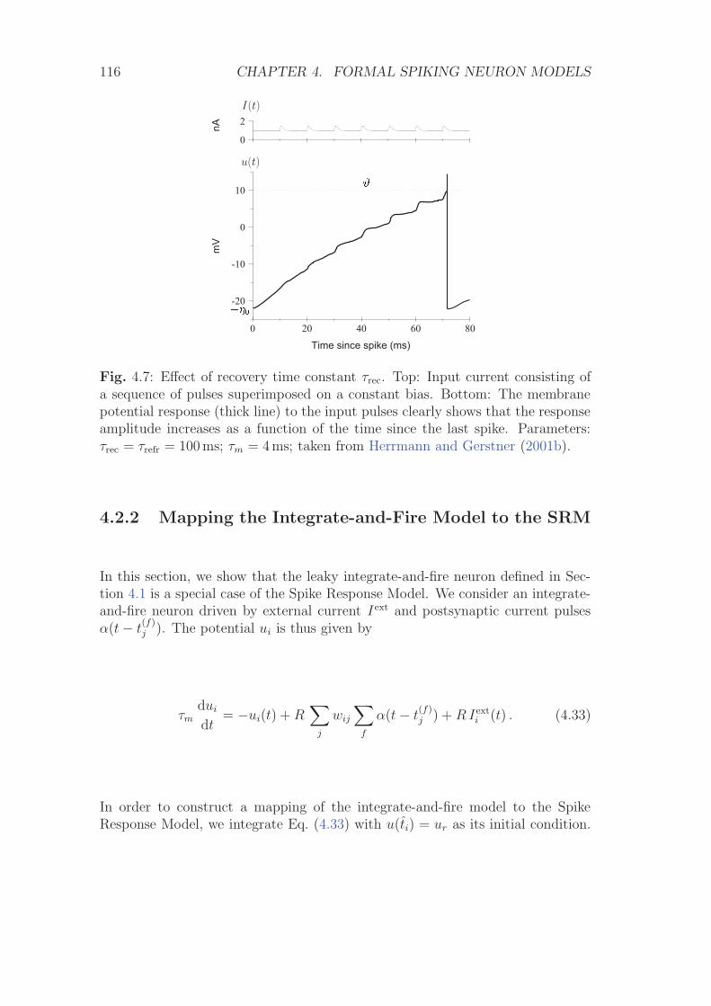
116 CHAPTER 4. FORMAL SPIKING NEURON MODELS
0
2
nA
0 20 40 60 80
-20
-10
0
10
Time since spike (ms)
mV
�
�����
I(t)
u(t)
Fig. 4.7: Effect of recovery time constant τrec. Top: Input current consisting ofa sequence of pulses superimposed on a constant bias. Bottom: The membranepotential response (thick line) to the input pulses clearly shows that the responseamplitude increases as a function of the time since the last spike. Parameters:τrec = τrefr = 100ms; τm = 4ms; taken from Herrmann and Gerstner (2001b).
4.2.2 Mapping the Integrate-and-Fire Model to the SRM
In this section, we show that the leaky integrate-and-fire neuron defined in Sec-tion 4.1 is a special case of the Spike Response Model. We consider an integrate-and-fire neuron driven by external current Iext and postsynaptic current pulsesα(t− t
(f)j ). The potential ui is thus given by
τmdui
dt= −ui(t) + R
∑j
wij
∑f
α(t− t(f)j ) + R Iext
i (t) . (4.33)
In order to construct a mapping of the integrate-and-fire model to the SpikeResponse Model, we integrate Eq. (4.33) with u(ti) = ur as its initial condition.
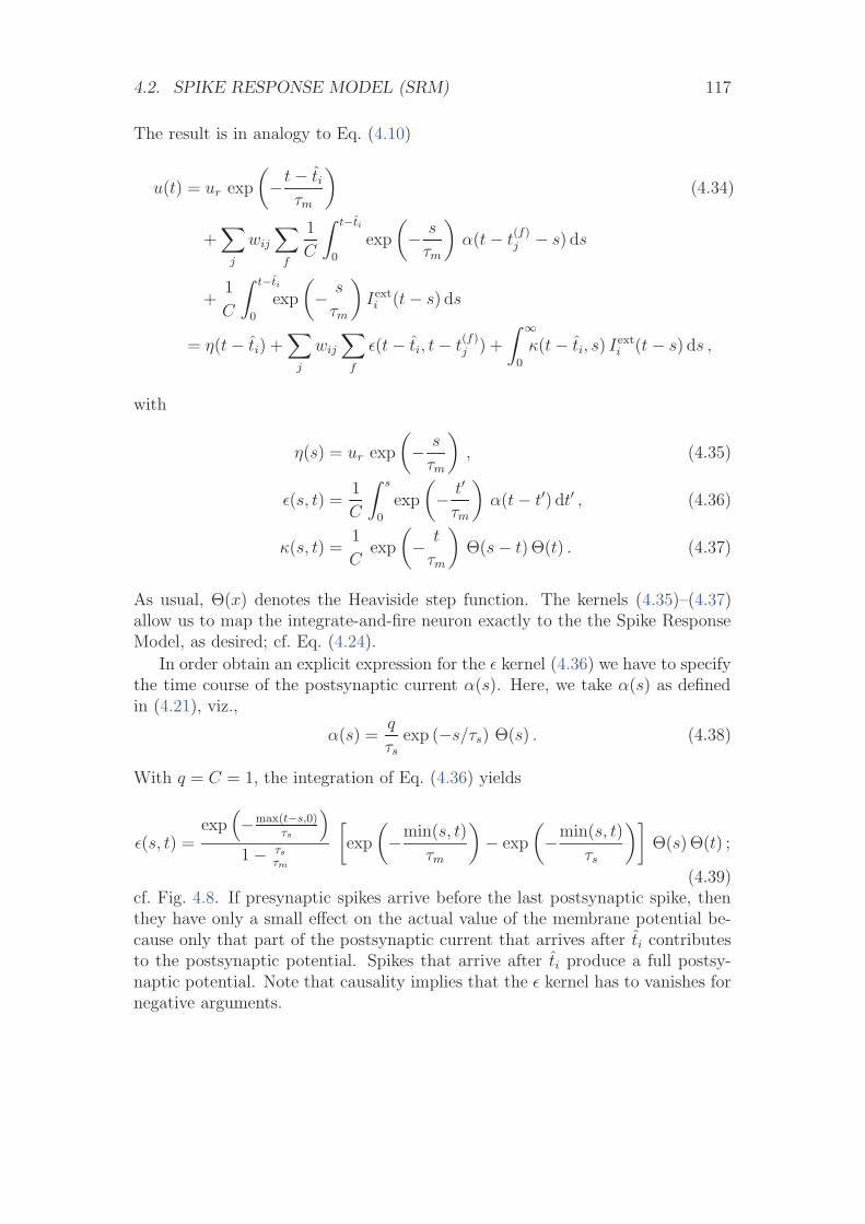
4.2. SPIKE RESPONSE MODEL (SRM) 117
The result is in analogy to Eq. (4.10)
u(t) = ur exp
(−t− ti
τm
)(4.34)
+∑
j
wij
∑f
1
C
∫ t−ti
0
exp
(− s
τm
)α(t− t
(f)j − s) ds
+1
C
∫ t−ti
0
exp
(− s
τm
)Iexti (t− s) ds
= η(t− ti) +∑
j
wij
∑f
ε(t− ti, t− t(f)j ) +
∫ ∞
0
κ(t− ti, s) Iexti (t− s) ds ,
with
η(s) = ur exp
(− s
τm
), (4.35)
ε(s, t) =1
C
∫ s
0
exp
(− t′
τm
)α(t− t′) dt′ , (4.36)
κ(s, t) =1
Cexp
(− t
τm
)Θ(s− t) Θ(t) . (4.37)
As usual, Θ(x) denotes the Heaviside step function. The kernels (4.35)–(4.37)allow us to map the integrate-and-fire neuron exactly to the the Spike ResponseModel, as desired; cf. Eq. (4.24).
In order obtain an explicit expression for the ε kernel (4.36) we have to specifythe time course of the postsynaptic current α(s). Here, we take α(s) as definedin (4.21), viz.,
α(s) =q
τsexp (−s/τs) Θ(s) . (4.38)
With q = C = 1, the integration of Eq. (4.36) yields
ε(s, t) =exp
(−max(t−s,0)
τs
)1− τs
τm
[exp
(−min(s, t)
τm
)− exp
(−min(s, t)
τs
)]Θ(s) Θ(t) ;
(4.39)cf. Fig. 4.8. If presynaptic spikes arrive before the last postsynaptic spike, thenthey have only a small effect on the actual value of the membrane potential be-cause only that part of the postsynaptic current that arrives after ti contributesto the postsynaptic potential. Spikes that arrive after ti produce a full postsy-naptic potential. Note that causality implies that the ε kernel has to vanishes fornegative arguments.
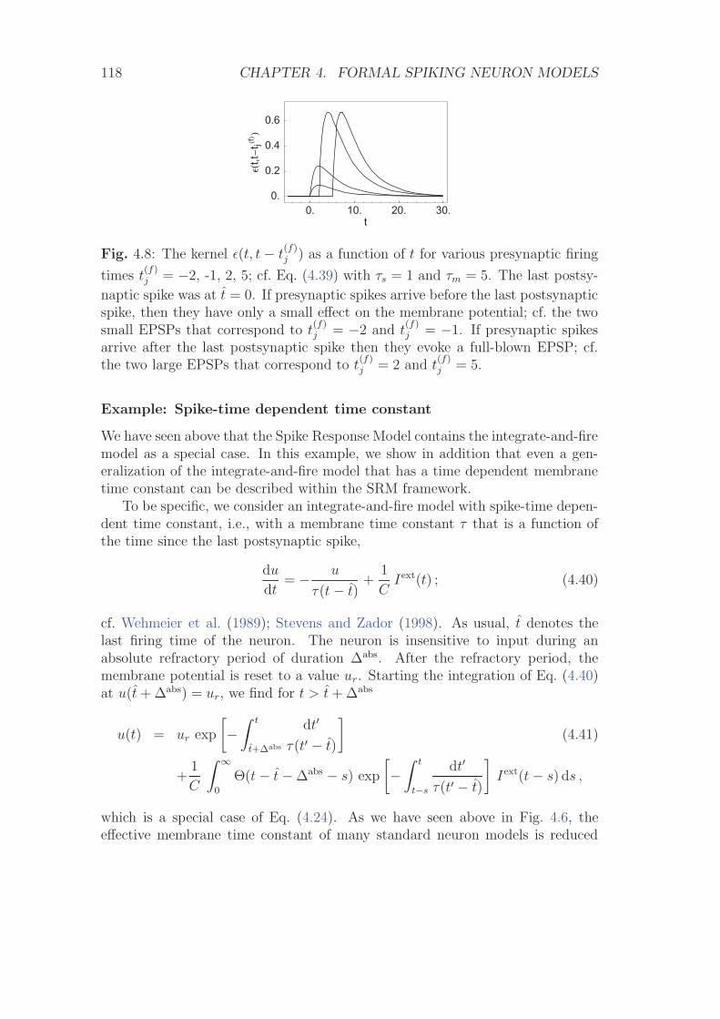
118 CHAPTER 4. FORMAL SPIKING NEURON MODELS
0. 10. 20. 30.t
0.
0.2
0.4
0.6
Ε�t,t�
t j�f��
Fig. 4.8: The kernel ε(t, t− t(f)j ) as a function of t for various presynaptic firing
times t(f)j = −2, -1, 2, 5; cf. Eq. (4.39) with τs = 1 and τm = 5. The last postsy-
naptic spike was at t = 0. If presynaptic spikes arrive before the last postsynapticspike, then they have only a small effect on the membrane potential; cf. the twosmall EPSPs that correspond to t
(f)j = −2 and t
(f)j = −1. If presynaptic spikes
arrive after the last postsynaptic spike then they evoke a full-blown EPSP; cf.the two large EPSPs that correspond to t
(f)j = 2 and t
(f)j = 5.
Example: Spike-time dependent time constant
We have seen above that the Spike Response Model contains the integrate-and-firemodel as a special case. In this example, we show in addition that even a gen-eralization of the integrate-and-fire model that has a time dependent membranetime constant can be described within the SRM framework.
To be specific, we consider an integrate-and-fire model with spike-time depen-dent time constant, i.e., with a membrane time constant τ that is a function ofthe time since the last postsynaptic spike,
du
dt= − u
τ(t − t)+
1
CIext(t) ; (4.40)
cf. Wehmeier et al. (1989); Stevens and Zador (1998). As usual, t denotes thelast firing time of the neuron. The neuron is insensitive to input during anabsolute refractory period of duration Δabs. After the refractory period, themembrane potential is reset to a value ur. Starting the integration of Eq. (4.40)at u(t + Δabs) = ur, we find for t > t + Δabs
u(t) = ur exp
[−∫ t
t+Δabs
dt′
τ(t′ − t)
](4.41)
+1
C
∫ ∞
0
Θ(t− t−Δabs − s) exp
[−∫ t
t−s
dt′
τ(t′ − t)
]Iext(t− s) ds ,
which is a special case of Eq. (4.24). As we have seen above in Fig. 4.6, theeffective membrane time constant of many standard neuron models is reduced
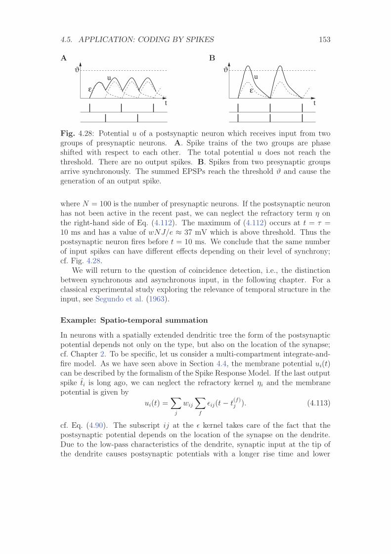
4.5. APPLICATION: CODING BY SPIKES 153
A
t
uε
ϑB
t
ϑ
ε
u
Fig. 4.28: Potential u of a postsynaptic neuron which receives input from twogroups of presynaptic neurons. A. Spike trains of the two groups are phaseshifted with respect to each other. The total potential u does not reach thethreshold. There are no output spikes. B. Spikes from two presynaptic groupsarrive synchronously. The summed EPSPs reach the threshold ϑ and cause thegeneration of an output spike.
where N = 100 is the number of presynaptic neurons. If the postsynaptic neuronhas not been active in the recent past, we can neglect the refractory term η onthe right-hand side of Eq. (4.112). The maximum of (4.112) occurs at t = τ =10 ms and has a value of wNJ/e ≈ 37 mV which is above threshold. Thus thepostsynaptic neuron fires before t = 10 ms. We conclude that the same numberof input spikes can have different effects depending on their level of synchrony;cf. Fig. 4.28.
We will return to the question of coincidence detection, i.e., the distinctionbetween synchronous and asynchronous input, in the following chapter. For aclassical experimental study exploring the relevance of temporal structure in theinput, see Segundo et al. (1963).
Example: Spatio-temporal summation
In neurons with a spatially extended dendritic tree the form of the postsynapticpotential depends not only on the type, but also on the location of the synapse;cf. Chapter 2. To be specific, let us consider a multi-compartment integrate-and-fire model. As we have seen above in Section 4.4, the membrane potential ui(t)can be described by the formalism of the Spike Response Model. If the last outputspike ti is long ago, we can neglect the refractory kernel ηi and the membranepotential is given by
ui(t) =∑
j
wij
∑f
εij(t− t(f)j ). (4.113)
cf. Eq. (4.90). The subscript ij at the ε kernel takes care of the fact that thepostsynaptic potential depends on the location of the synapse on the dendrite.Due to the low-pass characteristics of the dendrite, synaptic input at the tip ofthe dendrite causes postsynaptic potentials with a longer rise time and lower
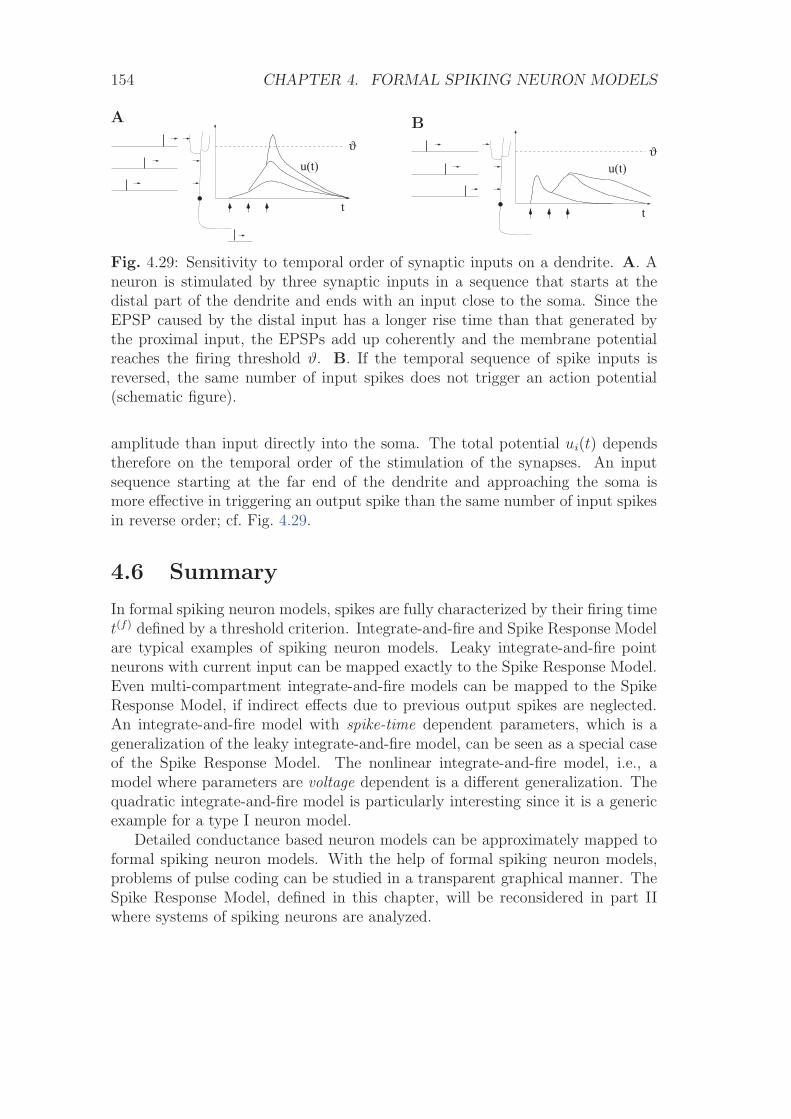
154 CHAPTER 4. FORMAL SPIKING NEURON MODELS
A
u(t)
t
ϑ
B
u(t)
t
ϑ
Fig. 4.29: Sensitivity to temporal order of synaptic inputs on a dendrite. A. Aneuron is stimulated by three synaptic inputs in a sequence that starts at thedistal part of the dendrite and ends with an input close to the soma. Since theEPSP caused by the distal input has a longer rise time than that generated bythe proximal input, the EPSPs add up coherently and the membrane potentialreaches the firing threshold ϑ. B. If the temporal sequence of spike inputs isreversed, the same number of input spikes does not trigger an action potential(schematic figure).
amplitude than input directly into the soma. The total potential ui(t) dependstherefore on the temporal order of the stimulation of the synapses. An inputsequence starting at the far end of the dendrite and approaching the soma ismore effective in triggering an output spike than the same number of input spikesin reverse order; cf. Fig. 4.29.
4.6 Summary
In formal spiking neuron models, spikes are fully characterized by their firing timet(f) defined by a threshold criterion. Integrate-and-fire and Spike Response Modelare typical examples of spiking neuron models. Leaky integrate-and-fire pointneurons with current input can be mapped exactly to the Spike Response Model.Even multi-compartment integrate-and-fire models can be mapped to the SpikeResponse Model, if indirect effects due to previous output spikes are neglected.An integrate-and-fire model with spike-time dependent parameters, which is ageneralization of the leaky integrate-and-fire model, can be seen as a special caseof the Spike Response Model. The nonlinear integrate-and-fire model, i.e., amodel where parameters are voltage dependent is a different generalization. Thequadratic integrate-and-fire model is particularly interesting since it is a genericexample for a type I neuron model.
Detailed conductance based neuron models can be approximately mapped toformal spiking neuron models. With the help of formal spiking neuron models,problems of pulse coding can be studied in a transparent graphical manner. TheSpike Response Model, defined in this chapter, will be reconsidered in part IIwhere systems of spiking neurons are analyzed.

4.6. SUMMARY 155
Literature
Formal neuron models where spikes are triggered by a threshold process havebeen popular in the sixties (Stein, 1965, 1967b; Geisler and Goldberg, 1966;Weiss, 1966), but the ideas can be traced back much further (Lapicque, 1907;Hill, 1936). It has been recognized early that these models lend themselves forhardware implementations (French and Stein, 1970) and mathematical analysis(Stein, 1965, 1967a), and can be fitted to experimental data (Brillinger, 1988,1992). Recent developments in computation and coding with formal spiking neu-rons has been reviewed in the book ‘Pulsed Neural Networks’ edited by Maassand Bishop (1998).

156 CHAPTER 4. FORMAL SPIKING NEURON MODELS
Chapter 5
Noise in Spiking Neuron Models
In vivo recordings of neuronal activity are characterized by a high degree ofirregularity. The spike train of individual neurons is far from being periodic andrelations between the firing patterns of several neurons seem to be random. Ifthe electrical activity picked up by an extra-cellular electrode is made audibleby a loudspeaker then we basically hear – noise. The question whether this isindeed just noise or rather a highly efficient way of coding information cannoteasily be answered. Listening to a computer modem or a fax machine might alsoleave the impression that this is just noise. Being able to decide whether we arewitnessing the neuronal activity that is underlying the composition of a poem (orthe electronic transmission of a love letter) and not just meaningless noise is oneof the most burning problems in Neuroscience.
Several experiments have been undertaken to tackle this problem. It seemsas if neurons can react in a very reliable and reproducible manner to fluctuat-ing currents that are injected via intracellular electrodes. As long as the sametime-course of the injected current is used the action potentials occur with pre-cisely the same timing relative to the stimulation (Mainen and Sejnowski, 1995;Bryant and Segundo, 1976). A related phenomenon can be observed by usingnon-stationary sensory stimulation. Spatially uniform random flicker, for exam-ple, elicits more or less the same spike train in retinal ganglion cells if the sameflicker sequence is presented again (Berry et al., 1997). A similar behavior hasbeen reported for motion-sensitive neurons of the visual system in flies (de Ruytervan Steveninck et al., 1997) and monkey cortex (Bair and Koch, 1996). On theother hand, neurons produce irregular spike trains in the absence of any tempo-rally structured stimuli. Irregular spontaneous activity, i.e., activity that is notrelated in any obvious way to external stimulation, and trial-to-trial variations inneuronal responses are often considered as noise (Softky and Koch, 1993; Shadlenand Newsome, 1994).
The origin of the irregularity in the electrical activity of cortical neurons invivo is poorly understood. In spiking neuron models such as the integrate-and-
157
158 CHAPTER 5. NOISE IN SPIKING NEURON MODELS
fire or Spike Response Model (SRM), noise is therefore often added explicitly toneuronal dynamics so as to mimic the unpredictability of neuronal recordings.In this chapter we present three different ways to implement noise in models ofneuronal networks, viz. escape noise (Section 5.3), slow noise in the parameters(Section 5.4), and diffusive noise (Section 5.5). In Section 5.6 we discuss thedifferences between subthreshold and superthreshold stimulation and explain itsconsequences for spike train variability. In the subthreshold regime, it is possibleto relate the diffusive noise model to the escape noise model. Section 5.7 illus-trates this relation. The noise models are finally applied to the phenomenon ofstochastic resonance in Section 5.8 and compared with rate models in Section 5.9.Before we start with the discussion of the noise models, we review in Section 5.1some experimental evidence for noise in neurons and introduce in Section 5.2 astatistical framework of spike train analysis.
5.1 Spike train variability
If neuron models such as the Hodgkin-Huxley or the integrate-and-fire model aredriven by a sufficiently strong constant current, they generate a regular sequenceof spikes. In neuronal models with adaptation currents1 there might be a shorttransient phase at the beginning, but then all interspike intervals are constant.Spike trains of typical neurons in vivo show a much more irregular behavior.Whether the irregularity is the sign of noise or of a rich code is at present an openquestion (Softky and Koch, 1993; Shadlen and Newsome, 1994; Bair and Koch,1996). In the first subsection we review some evidence for neuronal variabilityand spike train irregularity. We then discuss potential sources of noise.
5.1.1 Are neurons noisy?
Many in vivo experiments show noisy behavior of central neurons. The activityof neurons from the visual cortex, for example, can be recorded while a slowlymoving bar is presented on a screen within the visual field of the animal (Hubeland Wiesel, 1959, 1977). As soon as the bar enters the neuron’s receptive fieldthe firing rate goes up until the bar leaves the receptive field at the oppositeborder. The spike train, however, varies considerably from trial to trial, if thesame experiment is repeated several times. Furthermore, the very same neuronis spontaneously active even if the screen is blank and no external stimulus isapplied. During spontaneous activity, the intervals between one spike and thenext exhibit a large variability resulting in a broad distribution of interspikeintervals; see e.g., Softky and Koch (1993).
1We neglect here intrinsically bursting and chaotic neurons.

Part II
Population Models
211

Chapter 6
Population Equations
In many areas of the brain neurons are organized in populations of units withsimilar properties. Prominent examples are columns in the somatosensory andvisual cortex (Mountcastle, 1957; Hubel and Wiesel, 1962) and pools of motorneurons (Kandel and Schwartz, 1991). Given the large number of neurons withinsuch a column or pool it is sensible to describe the mean activity of the neuronalpopulation rather than the spiking of individual neurons. The idea of a popula-tion activity has already been introduced in Chapter 1.4. In a population of Nneurons, we calculate the proportion of active neurons by counting the numberof spikes nact(t; t + Δt) in a small time interval Δt and dividing by N . Furtherdivision by Δt yields the population activity
A(t) = limΔt→01
Δt
nact(t; t + Δt)
N=
1
N
N∑j=1
∑f
δ(t− t(f)j ) (6.1)
where δ denotes the Dirac δ function. The double sum runs over all firing timest(f)j of all neurons in the population. In other words the activity A is defined by a
population average. Even though the activity has units of a rate, the populationactivity is quite different from a mean firing rate defined by temporal average; cf.Chapter 1.4.
Theories of population activity have a long tradition (Knight, 1972a; Wilsonand Cowan, 1972, 1973; Amari, 1974; Abbott and van Vreeswijk, 1993; Gerstnerand van Hemmen, 1992; Treves, 1993; Gerstner, 1995; Amit and Brunel, 1997a,b;Brunel and Hakim, 1999; Fusi and Mattia, 1999; Brunel, 2000; Gerstner, 2000b;Nykamp and Tranchina, 2000; Omurtag et al., 2000; Eggert and van Hemmen,2001). In this chapter we study the properties of a large and homogeneous pop-ulation of spiking neurons. Why do we restrict ourselves to large populations? Ifwe repeatedly conduct the same experiment on a population of, say, one hundredpotentially noisy neurons, the observed activity A(t) defined in Eq. (6.1) will varyfrom one trial to the next. Therefore we cannot expect a population theory to
213
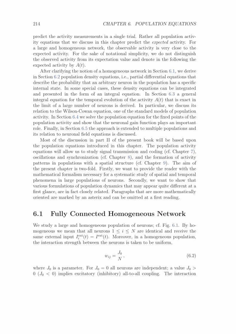
214 CHAPTER 6. POPULATION EQUATIONS
predict the activity measurements in a single trial. Rather all population activ-ity equations that we discuss in this chapter predict the expected activity. Fora large and homogeneous network, the observable activity is very close to theexpected activity. For the sake of notational simplicity, we do not distinguishthe observed activity from its expectation value and denote in the following theexpected activity by A(t).
After clarifying the notion of a homogeneous network in Section 6.1, we derivein Section 6.2 population density equations, i.e., partial differential equations thatdescribe the probability that an arbitrary neuron in the population has a specificinternal state. In some special cases, these density equations can be integratedand presented in the form of an integral equation. In Section 6.3 a generalintegral equation for the temporal evolution of the activity A(t) that is exact inthe limit of a large number of neurons is derived. In particular, we discuss itsrelation to the Wilson-Cowan equation, one of the standard models of populationactivity. In Section 6.4 we solve the population equation for the fixed points of thepopulation activity and show that the neuronal gain function plays an importantrole. Finally, in Section 6.5 the approach is extended to multiple populations andits relation to neuronal field equations is discussed.
Most of the discussion in part II of the present book will be based uponthe population equations introduced in this chapter. The population activityequations will allow us to study signal transmission and coding (cf. Chapter 7),oscillations and synchronization (cf. Chapter 8), and the formation of activitypatterns in populations with a spatial structure (cf. Chapter 9). The aim ofthe present chapter is two-fold. Firstly, we want to provide the reader with themathematical formalism necessary for a systematic study of spatial and temporalphenomena in large populations of neurons. Secondly, we want to show thatvarious formulations of population dynamics that may appear quite different at afirst glance, are in fact closely related. Paragraphs that are more mathematicallyoriented are marked by an asterix and can be omitted at a first reading.
6.1 Fully Connected Homogeneous Network
We study a large and homogeneous population of neurons; cf. Fig. 6.1. By ho-mogeneous we mean that all neurons 1 ≤ i ≤ N are identical and receive thesame external input Iext
i (t) = Iext(t). Moreover, in a homogeneous population,the interaction strength between the neurons is taken to be uniform,
wij =J0
N, (6.2)
where J0 is a parameter. For J0 = 0 all neurons are independent; a value J0 >0 (J0 < 0) implies excitatory (inhibitory) all-to-all coupling. The interaction
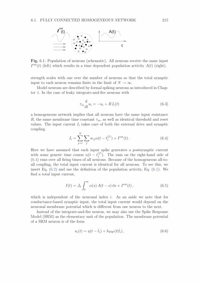
6.1. FULLY CONNECTED HOMOGENEOUS NETWORK 215
A(t)
t
I (t)ext
Fig. 6.1: Population of neurons (schematic). All neurons receive the same inputIext(t) (left) which results in a time dependent population activity A(t) (right).
strength scales with one over the number of neurons so that the total synapticinput to each neuron remains finite in the limit of N →∞.
Model neurons are described by formal spiking neurons as introduced in Chap-ter 4. In the case of leaky integrate-and-fire neurons with
τmd
dtui = −ui + R Ii(t) (6.3)
a homogeneous network implies that all neurons have the same input resistanceR, the same membrane time constant τm, as well as identical threshold and resetvalues. The input current Ii takes care of both the external drive and synapticcoupling
Ii =N∑
j=1
∑f
wijα(t− t(f)j ) + Iext(t) . (6.4)
Here we have assumed that each input spike generates a postsynaptic currentwith some generic time course α(t − t
(f)j ). The sum on the right-hand side of
(6.4) runs over all firing times of all neurons. Because of the homogeneous all-to-all coupling, the total input current is identical for all neurons. To see this, weinsert Eq. (6.2) and use the definition of the population activity, Eq. (6.1). Wefind a total input current,
I(t) = J0
∫ ∞
0
α(s) A(t− s) ds + Iext(t) , (6.5)
which is independent of the neuronal index i. As an aside we note that forconductance-based synaptic input, the total input current would depend on theneuronal membrane potential which is different from one neuron to the next.
Instead of the integrate-and-fire neuron, we may also use the Spike ResponseModel (SRM) as the elementary unit of the population. The membrane potentialof a SRM neuron is of the form
ui(t) = η(t− ti) + hPSP(t|ti) , (6.6)
Chapter 7
Signal Transmission andNeuronal Coding
In the preceding chapters, a theoretical description of neurons and neuronal popu-lations has been developed. We are now ready to apply the theoretical frameworkto one of the fundamental problems of Neuroscience – the problem of neuronalcoding and signal transmission. We will address the problem as three differentquestions, viz.,
(i) How does a population of neurons react to a fast change in the input? Thisquestion, which is particularly interesting in the context of reaction timeexperiments, is the topic of Section 7.2.
(ii) What is the response of an asynchronously firing population to an arbitrarytime-dependent input current? This question points to the signal transferproperties as a function of stimulation frequency and noise. In Section 7.3we calculate the signal transfer function for a large population as well as thesignal-to-noise ratio in a finite population of, say, a few hundred neurons.
(iii) What is the ‘meaning’ of a single spike? If a neuronal population receivesone extra input spike, how does this affect the population activity? Onthe other hand, if a neuron emits a spike, what do we learn about theinput? These questions, which are intimately related to the problem ofneural coding, are discussed in Section 7.4.
The population integral equation of Chapter 6.3 allows us to discuss thesequestions from a unified point of view. We focus in this chapter on a system ofidentical and independent neurons, i.e., a homogeneous network without lateralcoupling. In this case, the behavior of the population as a whole is identicalto the averaged behavior of a single neuron. Thus the signal transfer functiondiscussed in Section 7.3 or the coding characteristics discussed in Section 7.4 can
257
258 CHAPTER 7. SIGNAL TRANSMISSION AND NEURONAL CODING
also be interpreted as single-neuron properties. Before we dive into the mainarguments we derive in Section 7.1 the linearized population equation that willbe used throughout this chapter.
7.1 Linearized Population Equation
We consider a homogeneous population of independent neurons. All neuronsreceive the same current I(t) fluctuating about the mean I0. More specifically weset
I(t) = I0 + ΔI(t) . (7.1)
For small fluctuations, |ΔI| I0, we expect that the population activity staysclose to the value A0 that it would have for a constant current I0, i.e.,
A(t) = A0 + ΔA(t) , (7.2)
with |ΔA| A0. In that case, we may expand the right-hand side of the popu-lation equation A(t) =
∫ t
−∞ PI(t|t) A(t) dt into a Taylor series about A0 to linearorder in ΔA. In this section, we want to show that for spiking neuron models(either integrate-and-fire or SRM0 neurons) the linearized population equationcan be written in the form
ΔA(t) =
∫ t
−∞P0(t− t) ΔA(t) dt + A0
d
dt
∫ ∞
0
L(x) Δh(t− x) dx , (7.3)
where P0(t − t) is the interval distribution for constant input I0, L(x) is a real-valued function that plays the role of an integral kernel, and
Δh(t) =
∫ ∞
0
κ(s) ΔI(t− s) ds (7.4)
is the input potential generated by the time-dependent part of the input current.The first term of the right-hand side of Eq. (7.3) takes into account that previousperturbations ΔA(t) with t < t have an after-effect one inter-spike interval later.The second term describes the immediate response to a change in the inputpotential. If we want to understand the response of the population to an inputcurrent ΔI(t), we need to know the characteristics of the kernel L(x). The maintask of this section is therefore the calculation of L(x).
Here we give an overview of the main results that we will obtain in the presentchapter; explicit expressions for the kernel L(x) are presented in Tab. 7.1.
(i) In the low-noise limit, the kernel L(x) is a Dirac δ function. The dynamicsof the population activity ΔA has therefore a term proportional to thederivative of the input potential; cf. Eq. (7.3). We will see that this resultimplies a fast response ΔA to any change in the input.
7.1. LINEARIZED POPULATION EQUATION 259
(ii) For high noise, the kernel L(x) depends critically on the noise model. Fornoise that is slow compared to the intrinsic neuronal dynamics (e.g., noisein the reset or stochastic spike arrival in combination with a slow synaptictime constant) the kernel L(x) is similar to that in the noise-free case. Thusthe dynamics of ΔA is proportional to the derivative of the input potentialand therefore fast.
(iii) For a large amount of ‘fast’ noise (e.g., escape noise), the kernel L(x) isbroad so that the dynamics of the population activity is rather proportionalto the input potential than to its derivative; cf. Eq. (7.3). As we will see,this implies that the response to a change in the input is slow.
Results for escape noise and reset noise have been derived by Gerstner (2000b)while results for diffusive noise have been presented by Brunel et al. (2001) basedon a linearization of the membrane potential density equation (Brunel and Hakim,1999). The effect of slow noise in parameters has already been discussed in Knight(1972a). Apart from the approach discussed in this section, a fast response of apopulation of integrate-and-fire neurons with diffusive noise can also be inducedif the variance of the diffusive noise is changed (Lindner and Schimansky-Geier,2001; Bethge et al., 2001).
Before we turn to the general case, we will focus in Section 7.1.1 on a noise-free population. We will see why the dynamics of ΔA(t) has a contributionproportional to the derivative of the input potential. In Section 7.1.2 we derivethe general expression for the kernel L(x) and apply it to different situations.Readers not interested in the mathematical details may skip the remainder ofthis section and move directly to Section 7.2.
7.1.1 Noise-free Population Dynamics (*)
We start with a reduction of the population integral equation (6.75) to the noise-free case. In the limit of no noise, the input-dependent interval distributionPI(t | t) reduces to a Dirac δ function, i.e.,
PI(t | t) = δ[t− t− T (t)] . (7.5)
where T (t) is the inter-spike interval of a neuron that has fired its last spike attime t. If we insert Eq. (7.5) in the integral equation of the population activity,A(t) =
∫ t
−∞ PI(t|t) A(t) dt, we find
A(t) =
∫ t
−∞δ(t− t− T (t)) A(t) dt . (7.6)
The interval T (t) of a noise-free neuron is given implicitly by the threshold con-dition
T (t) = min{(t− t) | u(t) = ϑ; u > 0, t > t} . (7.7)
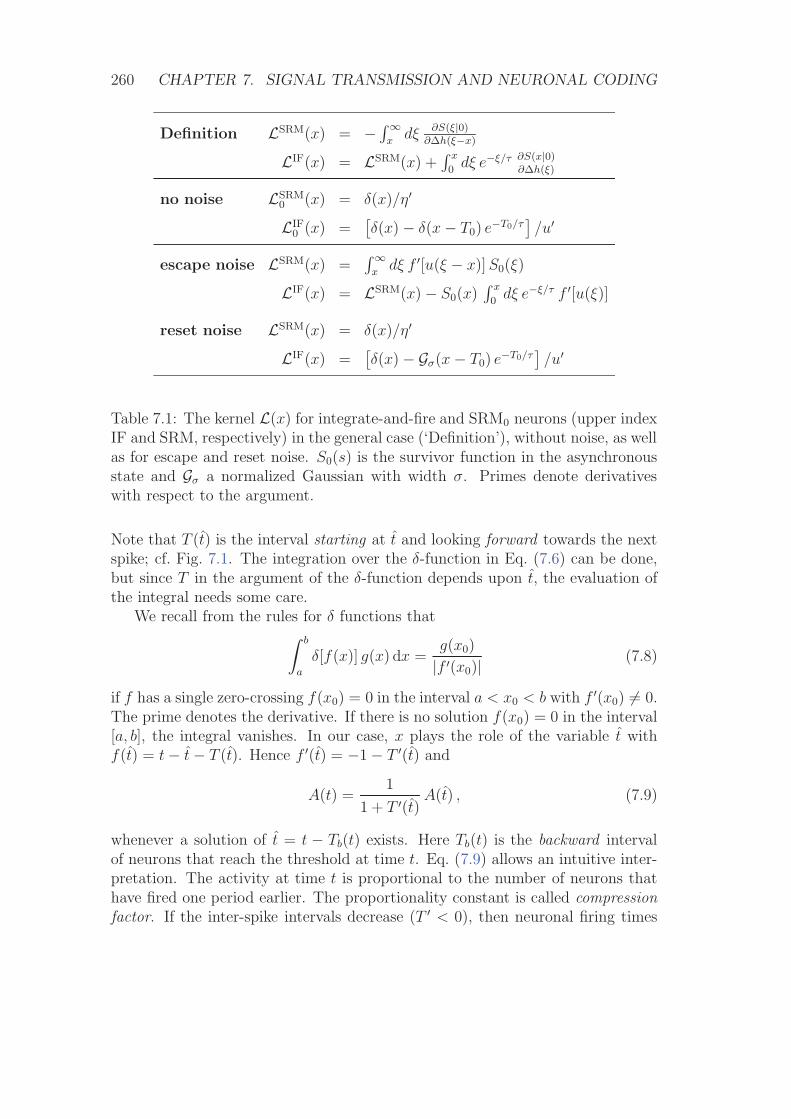
260 CHAPTER 7. SIGNAL TRANSMISSION AND NEURONAL CODING
Definition LSRM(x) = − ∫∞x
dξ ∂S(ξ|0)∂Δh(ξ−x)
LIF(x) = LSRM(x) +∫ x
0dξ e−ξ/τ ∂S(x|0)
∂Δh(ξ)
no noise LSRM0 (x) = δ(x)/η′
LIF0 (x) =
[δ(x)− δ(x− T0) e−T0/τ
]/u′
escape noise LSRM(x) =∫∞
xdξ f ′[u(ξ − x)] S0(ξ)
LIF(x) = LSRM(x)− S0(x)∫ x
0dξ e−ξ/τ f ′[u(ξ)]
reset noise LSRM(x) = δ(x)/η′
LIF(x) =[δ(x)− Gσ(x− T0) e−T0/τ
]/u′
Table 7.1: The kernel L(x) for integrate-and-fire and SRM0 neurons (upper indexIF and SRM, respectively) in the general case (‘Definition’), without noise, as wellas for escape and reset noise. S0(s) is the survivor function in the asynchronousstate and Gσ a normalized Gaussian with width σ. Primes denote derivativeswith respect to the argument.
Note that T (t) is the interval starting at t and looking forward towards the nextspike; cf. Fig. 7.1. The integration over the δ-function in Eq. (7.6) can be done,but since T in the argument of the δ-function depends upon t, the evaluation ofthe integral needs some care.
We recall from the rules for δ functions that∫ b
a
δ[f(x)] g(x) dx =g(x0)
|f ′(x0)| (7.8)
if f has a single zero-crossing f(x0) = 0 in the interval a < x0 < b with f ′(x0) �= 0.The prime denotes the derivative. If there is no solution f(x0) = 0 in the interval[a, b], the integral vanishes. In our case, x plays the role of the variable t withf(t) = t− t− T (t). Hence f ′(t) = −1− T ′(t) and
A(t) =1
1 + T ′(t)A(t) , (7.9)
whenever a solution of t = t − Tb(t) exists. Here Tb(t) is the backward intervalof neurons that reach the threshold at time t. Eq. (7.9) allows an intuitive inter-pretation. The activity at time t is proportional to the number of neurons thathave fired one period earlier. The proportionality constant is called compressionfactor. If the inter-spike intervals decrease (T ′ < 0), then neuronal firing times
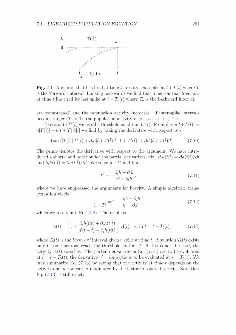
7.1. LINEARIZED POPULATION EQUATION 261
ϑ
t
T( t )u ^
T ( t )bt
Fig. 7.1: A neuron that has fired at time t fires its next spike at t+T (t) where Tis the ‘forward’ interval. Looking backwards we find that a neuron that fires nowat time t has fired its last spike at t− Tb(t) where Tb is the backward interval.
are ‘compressed’ and the population activity increases. If inter-spike intervalsbecome larger (T ′ > 0), the population activity decreases; cf. Fig. 7.2.
To evaluate T ′(t) we use the threshold condition (7.7). From ϑ = u[t+T (t)] =η[T (t)] + h[t + T (t)|t] we find by taking the derivative with respect to t
0 = η′[T (t)] T ′(t) + ∂th[t + T (t)|t] [1 + T ′(t)] + ∂th[t + T (t)|t] . (7.10)
The prime denotes the derivative with respect to the argument. We have intro-duced a short-hand notation for the partial derivatives, viz., ∂th(t|t) = ∂h(t|t)/∂tand ∂th(t|t) = ∂h(t|t)/∂t. We solve for T ′ and find
T ′ = −∂th + ∂th
η′ + ∂th, (7.11)
where we have suppressed the arguments for brevity. A simple algebraic trans-formation yields
1
1 + T ′= 1 +
∂th + ∂th
η′ − ∂th, (7.12)
which we insert into Eq. (7.9). The result is
A(t) =
[1 +
∂th(t|t) + ∂th(t|t)η′(t− t)− ∂th(t|t)
]A(t) , with t = t− Tb(t) , (7.13)
where Tb(t) is the backward interval given a spike at time t. A solution Tb(t) existsonly if some neurons reach the threshold at time t. If this is not the case, theactivity A(t) vanishes. The partial derivatives in Eq. (7.13) are to be evaluatedat t = t− Tb(t); the derivative η′ = dη(s)/ds is to be evaluated at s = Tb(t). Wemay summarize Eq. (7.13) by saying that the activity at time t depends on theactivity one period earlier modulated by the factor in square brackets. Note thatEq. (7.13) is still exact.
262 CHAPTER 7. SIGNAL TRANSMISSION AND NEURONAL CODING
Linearization
Let us consider a fluctuating input current that generates small perturbationsin the population activity ΔA(t) and the input potential Δh(t) as outlined atthe beginning of this section. If we substitute A(t) = A0 + ΔA(T ) and h(t|t) =h0 + δh(t|t) into Eq. (7.13) and linearize in ΔA and Δh we obtain an expressionof the form
ΔA(t) = ΔA(t− T ) + A0 C(t) , (7.14)
where T = 1/A0 is the interval for constant input I0 and C a time-dependentfactor, called compression factor. The activity at time t depends thus on theactivity one inter-spike interval earlier and on the instantanuous value of thecompression factor.
For SRM0 neurons we have h(t|t) = h(t) so that the partial derivative withrespect to t vanishes. The factor in square brackets in Eq. (7.13) reduces thereforeto [1 + (h′/η′)]. If we linearize Eq. (7.13) we find the compression factor
CSRM(t) = h′(t)/η′(T ) . (7.15)
For integrate-and-fire neurons we have a similar result. To evaluate the partialderivatives that we need in Eq. (7.13) we write u(t) = η(t− t) + h(t|t) with
η(t− t) = ur e−t−tτm
h(t|t) = h(t)− h(t) e−t−tτm ; (7.16)
cf. Eqs. (4.34) and (4.60). Here ur is the reset potential of the integrate-and-fireneurons and h(t) =
∫∞0
exp(−s/τm) I(t − s) ds is the input potential generatedby the input current I.
Taking the derivative of η and the partial derivatives of h yields
∂th + ∂th
η′ − ∂th=
h′(t)− h′(t− Tb) e−Tb/τm
h′(t− Tb) e−Tb/τm − τ−1m [ur + h(t− Tb)] e−Tb/τm
, (7.17)
which we now insert in Eq. (7.13). Since we are interested in the linearized activityequation, we replace Tb(t) by the interval T = 1/A0 for constant input and dropthe term h′ in the denominator. This yields Eq. (7.14) with a compression factorCIF given by
CIF(t) = [h′(t)− h′(t− T ) exp(−T/τm)]/u′ . (7.18)
Here u′ is the derivative of the membrane potential for constant input current I0,i.e., u′ = −τ−1
m [ur +h(t−Tb)] e−Tb/τm . The label IF is short for integrate-and-fire
neurons.
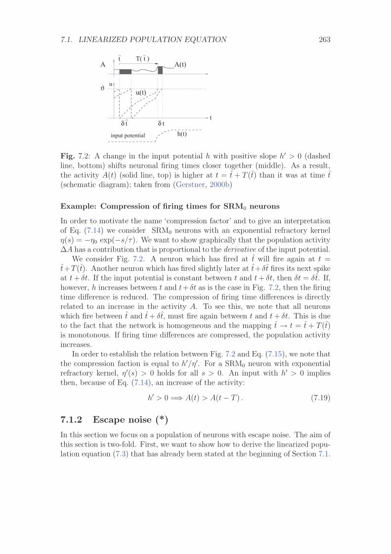
7.1. LINEARIZED POPULATION EQUATION 263
^
^
^
t
ϑu
t
A A(t)
u(t)
input potential h(t)δ t
t
δ
T( t )
Fig. 7.2: A change in the input potential h with positive slope h′ > 0 (dashedline, bottom) shifts neuronal firing times closer together (middle). As a result,the activity A(t) (solid line, top) is higher at t = t + T (t) than it was at time t(schematic diagram); taken from (Gerstner, 2000b)
Example: Compression of firing times for SRM0 neurons
In order to motivate the name ‘compression factor’ and to give an interpretationof Eq. (7.14) we consider SRM0 neurons with an exponential refractory kernelη(s) = −η0 exp(−s/τ). We want to show graphically that the population activityΔA has a contribution that is proportional to the derivative of the input potential.
We consider Fig. 7.2. A neuron which has fired at t will fire again at t =t+T (t). Another neuron which has fired slightly later at t+δt fires its next spikeat t + δt. If the input potential is constant between t and t + δt, then δt = δt. If,however, h increases between t and t+ δt as is the case in Fig. 7.2, then the firingtime difference is reduced. The compression of firing time differences is directlyrelated to an increase in the activity A. To see this, we note that all neuronswhich fire between t and t + δt, must fire again between t and t + δt. This is dueto the fact that the network is homogeneous and the mapping t → t = t + T (t)is monotonous. If firing time differences are compressed, the population activityincreases.
In order to establish the relation between Fig. 7.2 and Eq. (7.15), we note thatthe compression faction is equal to h′/η′. For a SRM0 neuron with exponentialrefractory kernel, η′(s) > 0 holds for all s > 0. An input with h′ > 0 impliesthen, because of Eq. (7.14), an increase of the activity:
h′ > 0 =⇒ A(t) > A(t− T ) . (7.19)
7.1.2 Escape noise (*)
In this section we focus on a population of neurons with escape noise. The aim ofthis section is two-fold. First, we want to show how to derive the linearized popu-lation equation (7.3) that has already been stated at the beginning of Section 7.1.
264 CHAPTER 7. SIGNAL TRANSMISSION AND NEURONAL CODING
Second, we will show that in the case of high noise the population activity followsthe input potential h(t), whereas for low noise the activity follows the derivativeh′(t). These results will be used in the following three sections for a discussion ofsignal transmission and coding properties.
In order to derive the linearized response ΔA of the population activity to achange in the input we start from the conservation law,
1 =
∫ t
−∞SI(t | t) A(t) dt , (7.20)
cf. (6.73). As we have seen in Chapter 6.3 the population equation (6.75) can beobtained by taking the derivative of Eq. (7.20) with respect to t, i.e.,
0 =d
dt
∫ t
−∞SI(t | t) A(t) dt . (7.21)
For constant input I0, the population activity has a constant value A0. Weconsider a small perturbation of the stationary state, A(t) = A0 + ΔA(t), that iscaused by a small change in the input current, ΔI(t). The time-dependent inputgenerates a total postsynaptic potential,
h(t|t) = h0(t|t) + Δh(t|t) , (7.22)
where h0(t|t) is the postsynaptic potential for constant input I0 and
Δh(t|t) =
∫ ∞
0
κ(t− t, s) ΔI(t− s) ds (7.23)
is the change of the postsynaptic potential generated by ΔI. We expand Eq. (7.21)to linear order in ΔA and Δh and find
0 =d
dt
∫ t
−∞S0(t− t) ΔA(t) dt
+ A0d
dt
{∫ t
−∞ds
∫ t
−∞dt Δh(s|t) ∂SI(t | t)
∂Δh(s|t)
∣∣∣∣Δh=0
}. (7.24)
We have used the notation S0(t − t) = SI0(t | t) for the survivor function of theasynchronous firing state. To take the derivative of the first term in Eq. (7.24)we use dS0(s)/ds = −P0(s) and S0(0) = 1. This yields
ΔA(t) =
∫ t
−∞P0(t− t) ΔA(t) dt
− A0d
dt
{∫ t
−∞ds
∫ t
−∞dt Δh(s|t) ∂SI(t | t)
∂Δh(s|t)
∣∣∣∣Δh=0
}. (7.25)
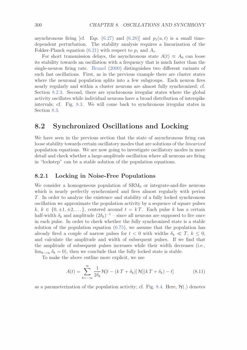
300 CHAPTER 8. OSCILLATIONS AND SYNCHRONY
asynchronous firing [cf. Eqs. (6.27) and (6.28)] and p1(u, t) is a small time-dependent perturbation. The stability analysis requires a linearization of theFokker-Planck equation (6.21) with respect to p1 and A1.
For short transmission delays, the asynchronous state A(t) ≡ A0 can looseits stability towards an oscillation with a frequency that is much faster than thesingle-neuron firing rate. Brunel (2000) distinguishes two different variants ofsuch fast oscillations. First, as in the previous example there are cluster stateswhere the neuronal population splits into a few subgroups. Each neuron firesnearly regularly and within a cluster neurons are almost fully synchronized; cf.Section 8.2.3. Second, there are synchronous irregular states where the globalactivity oscillates while individual neurons have a broad distribution of interspikeintervals; cf. Fig. 8.3. We will come back to synchronous irregular states inSection 8.3.
8.2 Synchronized Oscillations and Locking
We have seen in the previous section that the state of asynchronous firing canloose stability towards certain oscillatory modes that are solutions of the linearizedpopulation equations. We are now going to investigate oscillatory modes in moredetail and check whether a large-amplitude oscillation where all neurons are firingin “lockstep” can be a stable solution of the population equations.
8.2.1 Locking in Noise-Free Populations
We consider a homogeneous population of SRM0 or integrate-and-fire neuronswhich is nearly perfectly synchronized and fires almost regularly with periodT . In order to analyze the existence and stability of a fully locked synchronousoscillation we approximate the population activity by a sequence of square pulsesk, k ∈ {0,±1,±2, . . .}, centered around t = k T . Each pulse k has a certainhalf-width δk and amplitude (2δk)
−1 – since all neurons are supposed to fire oncein each pulse. In order to check whether the fully synchronized state is a stablesolution of the population equation (6.75), we assume that the population hasalready fired a couple of narrow pulses for t < 0 with widths δk T , k ≤ 0,and calculate the amplitude and width of subsequent pulses. If we find thatthe amplitude of subsequent pulses increases while their width decreases (i.e.,limk→∞ δk = 0), then we conclude that the fully locked state is stable.
To make the above outline more explicit, we use
A(t) =
∞∑k=−∞
1
2δkH[t− (k T + δk)]H[(k T + δk)− t] (8.11)
as a parameterization of the population activity; cf. Fig. 8.4. Here, H(.) denotes
8.2. SYNCHRONIZED OSCILLATIONS AND LOCKING 301
δ0
0 T 2T t
A(T)A(0)
2
Fig. 8.4: Sequence of rectangular activity pulses. If the fully synchronized stateis stable, the width δ of the pulses decreases while the amplitude increases.
the Heaviside step function with H(s) = 1 for s > 0 and H(s) = 0 for s ≤ 0.For stability, we need to show that the amplitude A(0), A(T ), A(2T ), . . . of therectangular pulses increases while the width δk of subsequent pulses decreases.
As we will see below, the condition for stable locking of all neurons in thepopulation can be stated as a condition on the slope of the input potential h atthe moment of firing. More precisely, if the last population pulse occurred atabout t = 0 with amplitude A(0) the amplitude of the population pulse at t = Tincreases, if h′(T ) > 0:
h′(T ) > 0 ⇐⇒ A(T ) > A(0) . (8.12)
If the amplitude of subsequent pulses increases, their width decreases. In otherwords, we have the following Locking Theorem. In a spatially homogeneous net-work of SRM0 or integrate-and-fire neurons, a necessary and, in the limit of a largenumber of presynaptic neurons (N →∞), also sufficient condition for a coherentoscillation to be asymptotically stable is that firing occurs when the postsynapticpotential arising from all previous spikes is increasing in time (Gerstner et al.,1996b).
The Locking Theorem is applicable for large populations that are alreadyclose to the fully synchronized state. A related but global locking argument hasbeen presented by (Mirollo and Strogatz, 1990). The locking argument can begeneralized to heterogeneous networks (Gerstner et al., 1993a; Chow, 1998) and toelectrical coupling (Chow and Kopell, 2000). Synchronization in small networkshas been discussed in, e.g., (Ernst et al., 1995; Chow, 1998; Hansel et al., 1995; vanVreeswijk et al., 1994; van Vreeswijk, 1996; Bose et al., 2000). For weak coupling,synchronization and locking can be systematically analyzed in the framework ofphase models (Kuramoto, 1975; Ermentrout and Kopell, 1984; Kopell, 1986) orcanonical neuron models (Hansel et al., 1995; Ermentrout, 1996; Hoppensteadtand Izhikevich, 1997; Izhikevich, 1999; Ermentrout et al., 2001).
Before we derive the locking condition for spiking neuron models, we illustratethe main idea by two examples.
Example: Perfect synchrony in noiseless SRM0 neurons
In this example we will show that locking in a population of spiking neuronscan be understood by simple geometrical arguments; there is no need to use the
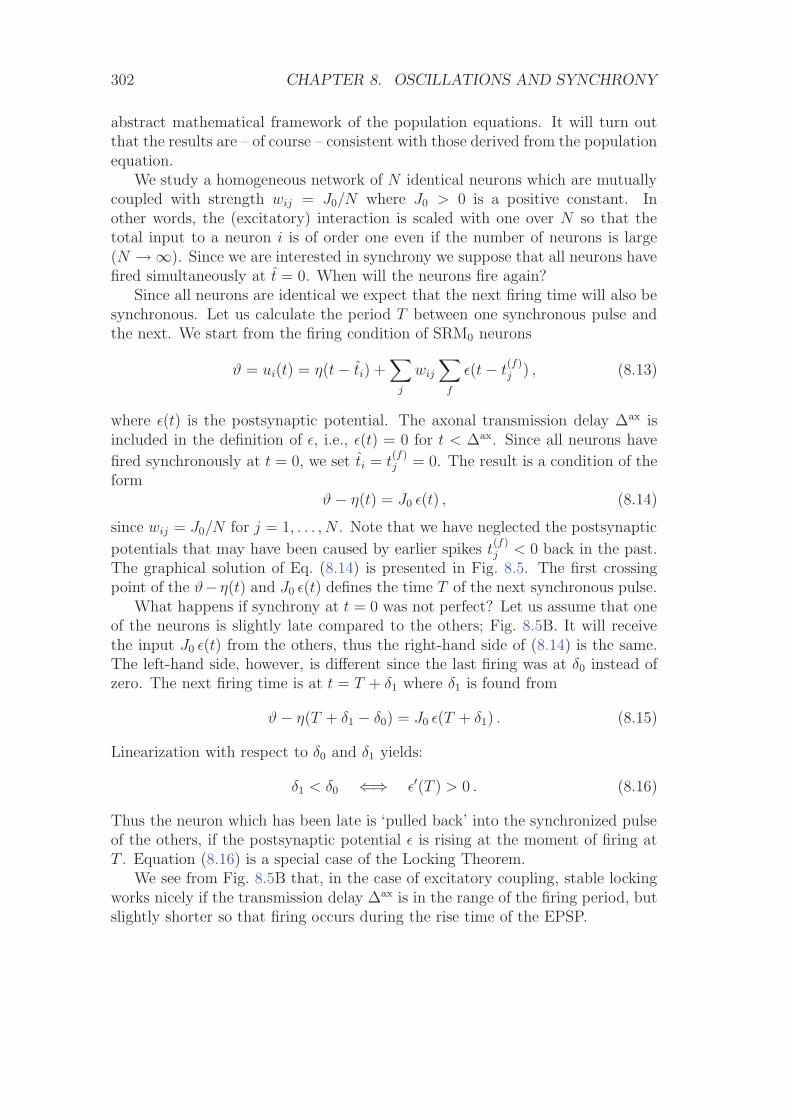
302 CHAPTER 8. OSCILLATIONS AND SYNCHRONY
abstract mathematical framework of the population equations. It will turn outthat the results are – of course – consistent with those derived from the populationequation.
We study a homogeneous network of N identical neurons which are mutuallycoupled with strength wij = J0/N where J0 > 0 is a positive constant. Inother words, the (excitatory) interaction is scaled with one over N so that thetotal input to a neuron i is of order one even if the number of neurons is large(N →∞). Since we are interested in synchrony we suppose that all neurons havefired simultaneously at t = 0. When will the neurons fire again?
Since all neurons are identical we expect that the next firing time will also besynchronous. Let us calculate the period T between one synchronous pulse andthe next. We start from the firing condition of SRM0 neurons
ϑ = ui(t) = η(t− ti) +∑
j
wij
∑f
ε(t− t(f)j ) , (8.13)
where ε(t) is the postsynaptic potential. The axonal transmission delay Δax isincluded in the definition of ε, i.e., ε(t) = 0 for t < Δax. Since all neurons have
fired synchronously at t = 0, we set ti = t(f)j = 0. The result is a condition of the
formϑ− η(t) = J0 ε(t) , (8.14)
since wij = J0/N for j = 1, . . . , N . Note that we have neglected the postsynaptic
potentials that may have been caused by earlier spikes t(f)j < 0 back in the past.
The graphical solution of Eq. (8.14) is presented in Fig. 8.5. The first crossingpoint of the ϑ−η(t) and J0 ε(t) defines the time T of the next synchronous pulse.
What happens if synchrony at t = 0 was not perfect? Let us assume that oneof the neurons is slightly late compared to the others; Fig. 8.5B. It will receivethe input J0 ε(t) from the others, thus the right-hand side of (8.14) is the same.The left-hand side, however, is different since the last firing was at δ0 instead ofzero. The next firing time is at t = T + δ1 where δ1 is found from
ϑ− η(T + δ1 − δ0) = J0 ε(T + δ1) . (8.15)
Linearization with respect to δ0 and δ1 yields:
δ1 < δ0 ⇐⇒ ε′(T ) > 0 . (8.16)
Thus the neuron which has been late is ‘pulled back’ into the synchronized pulseof the others, if the postsynaptic potential ε is rising at the moment of firing atT . Equation (8.16) is a special case of the Locking Theorem.
We see from Fig. 8.5B that, in the case of excitatory coupling, stable lockingworks nicely if the transmission delay Δax is in the range of the firing period, butslightly shorter so that firing occurs during the rise time of the EPSP.
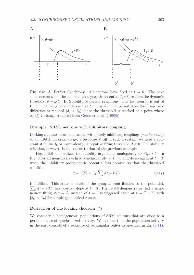
8.2. SYNCHRONIZED OSCILLATIONS AND LOCKING 303
A
tT0
u ϑ−η(t)
ε(t)J 0
B
0δ
t
ϑ−η δ
T
δ1
0
u
ε(t)
(t− ) 0
J 0
Fig. 8.5: A. Perfect Synchrony. All neurons have fired at t = 0. The nextspike occurs when the summed postsynaptic potential J0 ε(t) reaches the dynamicthreshold ϑ − η(t). B. Stability of perfect synchrony. The last neuron is out oftune. The firing time difference at t = 0 is δ0. One period later the firing timedifference is reduced (δ1 < δ0), since the threshold is reached at a point whereJ0ε(t) is rising. Adapted from Gerstner et al. (1996b).
Example: SRM0 neurons with inhibitory coupling
Locking can also occur in networks with purely inhibitory couplings (van Vreeswijket al., 1994). In order to get a response at all in such a system, we need a con-stant stimulus I0 or, equivalently, a negative firing threshold ϑ < 0. The stabilitycriterion, however, is equivalent to that of the previous example.
Figure 8.6 summarizes the stability arguments analogously to Fig. 8.5. InFig. 8.6A all neurons have fired synchronously at t = 0 and do so again at t = Twhen the inhibitory postsynaptic potential has decayed so that the thresholdcondition,
ϑ− η(T ) = J0
∑k
ε(t− k T ) , (8.17)
is fulfilled. This state is stable if the synaptic contribution to the potential,∑k ε(t− k T ), has positive slope at t = T . Figure 8.6 demonstrates that a single
neuron firing at t = δ0 instead of t = 0 is triggered again at t = T + δ1 with|δ1| < |δ0| for simple geometrical reasons.
Derivation of the locking theorem (*)
We consider a homogeneous populations of SRM neurons that are close to aperiodic state of synchronized activity. We assume that the population activityin the past consists of a sequence of rectangular pulses as specified in Eq. (8.11).
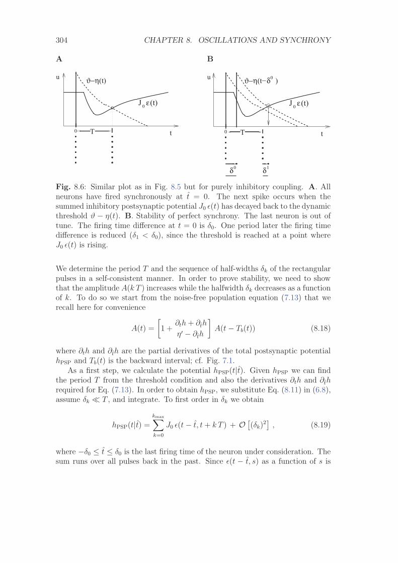
304 CHAPTER 8. OSCILLATIONS AND SYNCHRONY
A
tT0
u ϑ−η(t)
ε(t)J 0
B
0δ
t
ϑ−η δ
T
δ1
0
u
ε(t)
(t− ) 0
J 0
Fig. 8.6: Similar plot as in Fig. 8.5 but for purely inhibitory coupling. A. Allneurons have fired synchronously at t = 0. The next spike occurs when thesummed inhibitory postsynaptic potential J0 ε(t) has decayed back to the dynamicthreshold ϑ − η(t). B. Stability of perfect synchrony. The last neuron is out oftune. The firing time difference at t = 0 is δ0. One period later the firing timedifference is reduced (δ1 < δ0), since the threshold is reached at a point whereJ0 ε(t) is rising.
We determine the period T and the sequence of half-widths δk of the rectangularpulses in a self-consistent manner. In order to prove stability, we need to showthat the amplitude A(k T ) increases while the halfwidth δk decreases as a functionof k. To do so we start from the noise-free population equation (7.13) that werecall here for convenience
A(t) =
[1 +
∂th + ∂th
η′ − ∂th
]A(t− Tb(t)) (8.18)
where ∂th and ∂th are the partial derivatives of the total postsynaptic potentialhPSP and Tb(t) is the backward interval; cf. Fig. 7.1.
As a first step, we calculate the potential hPSP(t|t). Given hPSP we can findthe period T from the threshold condition and also the derivatives ∂th and ∂threquired for Eq. (7.13). In order to obtain hPSP, we substitute Eq. (8.11) in (6.8),assume δk T , and integrate. To first order in δk we obtain
hPSP(t|t) =kmax∑k=0
J0 ε(t− t, t + k T ) + O [(δk)
2]
, (8.19)
where −δ0 ≤ t ≤ δ0 is the last firing time of the neuron under consideration. Thesum runs over all pulses back in the past. Since ε(t − t, s) as a function of s is
Chapter 9
Spatially Structured Networks
So far the discussion of network behavior in Chapters 6 – 8 was restricted tohomogeneous populations of neurons. In this chapter we turn to networks thathave a spatial structure. In doing so we emphasize two characteristic featuresof the cerebral cortex, namely the high density of neurons and its virtually two-dimensional architecture.
Each cubic millimeter of cortical tissue contains about 105 neurons. Thisimpressive number suggests that a description of neuronal dynamics in terms ofan averaged population activity is more appropriate than a description on thesingle-neuron level. Furthermore, the cerebral cortex is huge. More precisely, theunfolded cerebral cortex of humans covers a surface of 2200–2400 cm2, but itsthickness amounts on average to only 2.5–3.0 mm2. If we do not look too closely,the cerebral cortex can hence be treated as a continuous two-dimensional sheet ofneurons. Neurons will no longer be labeled by discrete indices but by continuousvariables that give their spatial position on the sheet. The coupling of two neuronsi and j is replaced by the average coupling strength between neurons at position xand those at position y, or, even more radically simplified, by the average couplingstrength of two neurons being separated by the distance |x− y|. Similarly to thenotion of an average coupling strength we will also introduce the average activityof neurons located at position x and describe the dynamics of the network in termsof these averaged quantities only. The details of how these average quantities aredefined, are fairly involved and often disputable. In Sect. 9.1 we will – without aformal justification – introduce field equations for the spatial activity A(x, t) ina spatially extended, but otherwise homogeneous population of neurons. Thesefield equations are particularly interesting because they have solutions in the formof complex stationary patterns of activity, traveling waves, and rotating spirals –a phenomenology that is closely related to pattern formation in certain nonlinearsystems that are collectively termed excitable media. Some examples of thesesolutions are discussed in Sect. 9.1. In Sect. 9.2 we generalize the formalismso as to account for several distinct neuronal populations, such as those formed
323
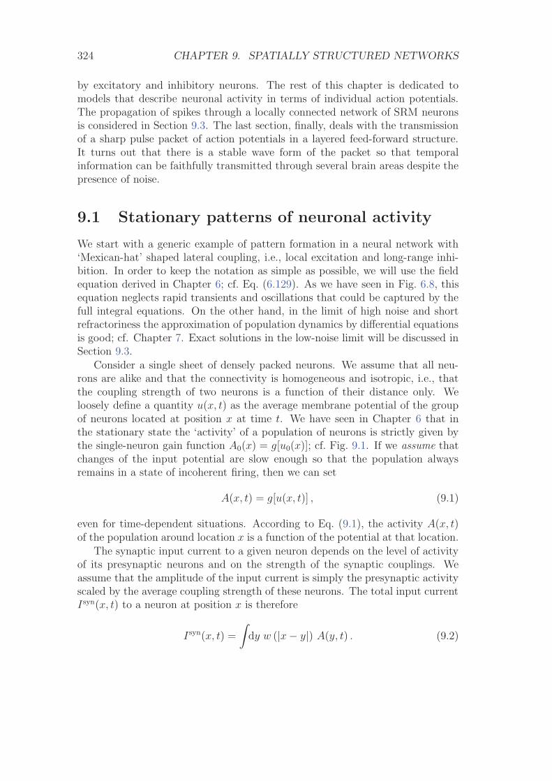
324 CHAPTER 9. SPATIALLY STRUCTURED NETWORKS
by excitatory and inhibitory neurons. The rest of this chapter is dedicated tomodels that describe neuronal activity in terms of individual action potentials.The propagation of spikes through a locally connected network of SRM neuronsis considered in Section 9.3. The last section, finally, deals with the transmissionof a sharp pulse packet of action potentials in a layered feed-forward structure.It turns out that there is a stable wave form of the packet so that temporalinformation can be faithfully transmitted through several brain areas despite thepresence of noise.
9.1 Stationary patterns of neuronal activity
We start with a generic example of pattern formation in a neural network with‘Mexican-hat’ shaped lateral coupling, i.e., local excitation and long-range inhi-bition. In order to keep the notation as simple as possible, we will use the fieldequation derived in Chapter 6; cf. Eq. (6.129). As we have seen in Fig. 6.8, thisequation neglects rapid transients and oscillations that could be captured by thefull integral equations. On the other hand, in the limit of high noise and shortrefractoriness the approximation of population dynamics by differential equationsis good; cf. Chapter 7. Exact solutions in the low-noise limit will be discussed inSection 9.3.
Consider a single sheet of densely packed neurons. We assume that all neu-rons are alike and that the connectivity is homogeneous and isotropic, i.e., thatthe coupling strength of two neurons is a function of their distance only. Weloosely define a quantity u(x, t) as the average membrane potential of the groupof neurons located at position x at time t. We have seen in Chapter 6 that inthe stationary state the ‘activity’ of a population of neurons is strictly given bythe single-neuron gain function A0(x) = g[u0(x)]; cf. Fig. 9.1. If we assume thatchanges of the input potential are slow enough so that the population alwaysremains in a state of incoherent firing, then we can set
A(x, t) = g[u(x, t)] , (9.1)
even for time-dependent situations. According to Eq. (9.1), the activity A(x, t)of the population around location x is a function of the potential at that location.
The synaptic input current to a given neuron depends on the level of activityof its presynaptic neurons and on the strength of the synaptic couplings. Weassume that the amplitude of the input current is simply the presynaptic activityscaled by the average coupling strength of these neurons. The total input currentIsyn(x, t) to a neuron at position x is therefore
Isyn(x, t) =
∫dy w (|x− y|) A(y, t) . (9.2)
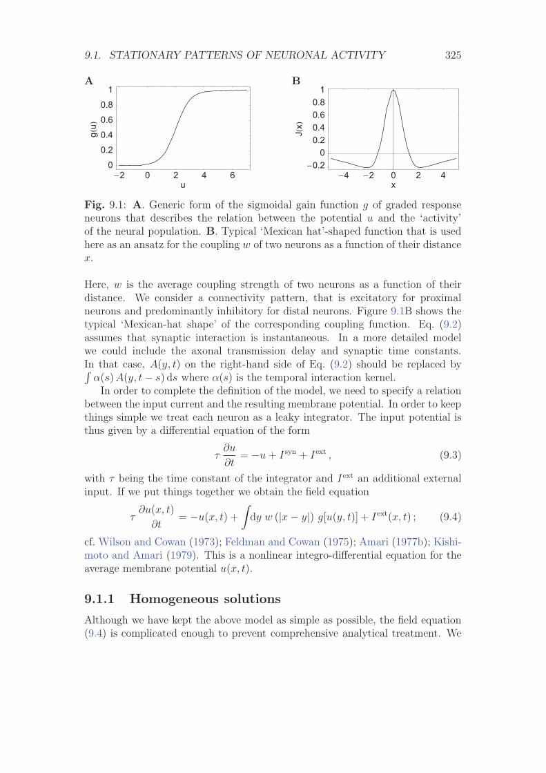
9.1. STATIONARY PATTERNS OF NEURONAL ACTIVITY 325
A
�2 0 2 4 6u
0
0.2
0.4
0.6
0.8
1g�
u�B
�4 �2 0 2 4x
�0.20
0.20.40.60.8
1
J�x�
Fig. 9.1: A. Generic form of the sigmoidal gain function g of graded responseneurons that describes the relation between the potential u and the ‘activity’of the neural population. B. Typical ‘Mexican hat’-shaped function that is usedhere as an ansatz for the coupling w of two neurons as a function of their distancex.
Here, w is the average coupling strength of two neurons as a function of theirdistance. We consider a connectivity pattern, that is excitatory for proximalneurons and predominantly inhibitory for distal neurons. Figure 9.1B shows thetypical ‘Mexican-hat shape’ of the corresponding coupling function. Eq. (9.2)assumes that synaptic interaction is instantaneous. In a more detailed modelwe could include the axonal transmission delay and synaptic time constants.In that case, A(y, t) on the right-hand side of Eq. (9.2) should be replaced by∫
α(s) A(y, t− s) ds where α(s) is the temporal interaction kernel.In order to complete the definition of the model, we need to specify a relation
between the input current and the resulting membrane potential. In order to keepthings simple we treat each neuron as a leaky integrator. The input potential isthus given by a differential equation of the form
τ∂u
∂t= −u + Isyn + Iext , (9.3)
with τ being the time constant of the integrator and I ext an additional externalinput. If we put things together we obtain the field equation
τ∂u(x, t)
∂t= −u(x, t) +
∫dy w (|x− y|) g[u(y, t)] + Iext(x, t) ; (9.4)
cf. Wilson and Cowan (1973); Feldman and Cowan (1975); Amari (1977b); Kishi-moto and Amari (1979). This is a nonlinear integro-differential equation for theaverage membrane potential u(x, t).
9.1.1 Homogeneous solutions
Although we have kept the above model as simple as possible, the field equation(9.4) is complicated enough to prevent comprehensive analytical treatment. We
326 CHAPTER 9. SPATIALLY STRUCTURED NETWORKS
therefore start our investigation by looking for a special type of solution, i.e., asolution that is uniform over space, but not necessarily constant over time. Wecall this the homogenous solution and write u(x, t) ≡ u(t). We expect that ahomogenous solution exists if the external input is homogeneous as well, i.e., ifIext(x, t) ≡ Iext(t).
Substitution of the ansatz u(x, t) ≡ u(t) into Eq. (9.4) yields
τdu(t)
dt= −u(t) + w g[u(t)] + Iext(t) . (9.5)
with w =∫
dy w (|y|). This is a nonlinear ordinary differential equation for theaverage membrane potential u(t). We note that the equation for the homogeneoussolution is identical to that of a single population without spatial structure; cf.Eq. (6.87) in Chapter 6.3.
The fixed points of the above equation with I ext = 0 are of particular interestbecause they correspond to a resting state of the network. More generally, wesearch for stationary solutions for a given constant external input I ext(x, t) ≡ Iext.The fixed points of Eq. (9.5) are solutions of
g(u) =u− Iext
w, (9.6)
which is represented graphically in Fig. 9.2. Depending on the strength of theexternal input three qualitatively different situations can be observed. For lowexternal stimulation there is a single fixed point at a very low level of neuronalactivity. This corresponds to a quiescent state where the activity of the wholenetwork has ceased. Large stimulation results in a fixed point at an almostsaturated level of activity which corresponds to a state where all neurons are firingat their maximum rate. Intermediate values of external stimulation, however, mayresult in a situation with more than one fixed point. Depending on the shapeof the output function and the mean synaptic coupling strength w three fixedpoints may appear. Two of them correspond to the quiescent and the highlyactivated state, respectively, which are separated by the third fixed point at anintermediate level of activity.
Any potential physical relevance of fixed points clearly depends on their sta-bility. Stability under the dynamics defined by the ordinary differential equationEq. (9.5) is readily checked using standard analysis. Stability requires that at theintersection
g′(u) < w−1 . (9.7)
Thus all fixed points corresponding to quiescent or highly activated states arestable whereas the middle fixed point in case of multiple solutions is unstable; cf.Fig. 9.2. This, however, is only half of the truth because Eq. (9.5) only describeshomogeneous solutions. Therefore, it may well be that the solutions are stable

Part III
Models of Synaptic Plasticity
359

Chapter 10
Hebbian Models
In the neuron models discussed so far each synapse is characterized by a sin-gle constant parameter wij that determines the amplitude of the postsynapticresponse to an incoming action potential. Electrophysiological experiments, how-ever, show that the response amplitude is not fixed but can change over time.Appropriate stimulation paradigms can systematically induce changes of the post-synaptic response that last for hours or days. If the stimulation paradigm leadsto a persistent increase of the synaptic transmission efficacy, the effect is calledlong-term potentiation of synapses, or LTP for short. If the result is a decreaseof the synaptic efficacy, it is called long-term depression (LTD). These persistentchanges are thought to be the neuronal correlate of ‘learning’ and ‘memory’.
In the formal theory of neural networks the weight wij of a connection fromneuron j to i is considered as a parameter that can be adjusted so as to optimizethe performance of a network for a given task. The process of parameter adap-tation is called learning and the procedure for adjusting the weights is referredto as a learning rule. Here learning is meant in its widest sense. It may referto synaptic changes during development just as well as to the specific changesnecessary to memorize a visual pattern or to learn a motor task. There are manydifferent learning rules that we cannot all cover in this book. In this chapter weconsider the simplest set of rules, viz., synaptic changes that are driven by corre-lated activity of pre- and postsynaptic neurons. This class of learning rule can bemotivated by Hebb’s principle and is therefore often called ‘Hebbian learning’.
10.1 Synaptic Plasticity
Over the last 30 years, a large body of experimental results on synaptic plasticityhas been accumulated. Many of these experiments are inspired by Hebb’s postu-late (Hebb, 1949) that describes how the connection from presynaptic neuron Ato a postsynaptic neuron B should be modified:
361
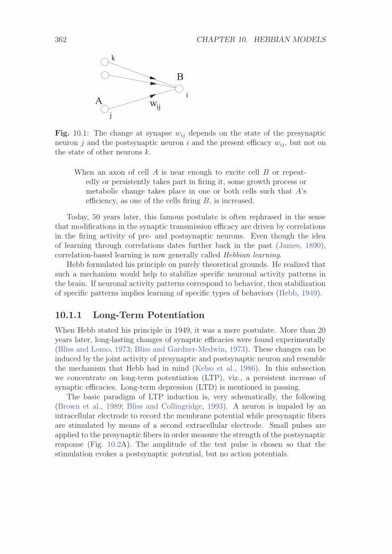
362 CHAPTER 10. HEBBIAN MODELS
A
B
ijwj
k
i
Fig. 10.1: The change at synapse wij depends on the state of the presynapticneuron j and the postsynaptic neuron i and the present efficacy wij, but not onthe state of other neurons k.
When an axon of cell A is near enough to excite cell B or repeat-edly or persistently takes part in firing it, some growth process ormetabolic change takes place in one or both cells such that A’sefficiency, as one of the cells firing B, is increased.
Today, 50 years later, this famous postulate is often rephrased in the sensethat modifications in the synaptic transmission efficacy are driven by correlationsin the firing activity of pre- and postsynaptic neurons. Even though the ideaof learning through correlations dates further back in the past (James, 1890),correlation-based learning is now generally called Hebbian learning.
Hebb formulated his principle on purely theoretical grounds. He realized thatsuch a mechanism would help to stabilize specific neuronal activity patterns inthe brain. If neuronal activity patterns correspond to behavior, then stabilizationof specific patterns implies learning of specific types of behaviors (Hebb, 1949).
10.1.1 Long-Term Potentiation
When Hebb stated his principle in 1949, it was a mere postulate. More than 20years later, long-lasting changes of synaptic efficacies were found experimentally(Bliss and Lomo, 1973; Bliss and Gardner-Medwin, 1973). These changes can beinduced by the joint activity of presynaptic and postsynaptic neuron and resemblethe mechanism that Hebb had in mind (Kelso et al., 1986). In this subsectionwe concentrate on long-term potentiation (LTP), viz., a persistent increase ofsynaptic efficacies. Long-term depression (LTD) is mentioned in passing.
The basic paradigm of LTP induction is, very schematically, the following(Brown et al., 1989; Bliss and Collingridge, 1993). A neuron is impaled by anintracellular electrode to record the membrane potential while presynaptic fibersare stimulated by means of a second extracellular electrode. Small pulses areapplied to the presynaptic fibers in order measure the strength of the postsynapticresponse (Fig. 10.2A). The amplitude of the test pulse is chosen so that thestimulation evokes a postsynaptic potential, but no action potentials.
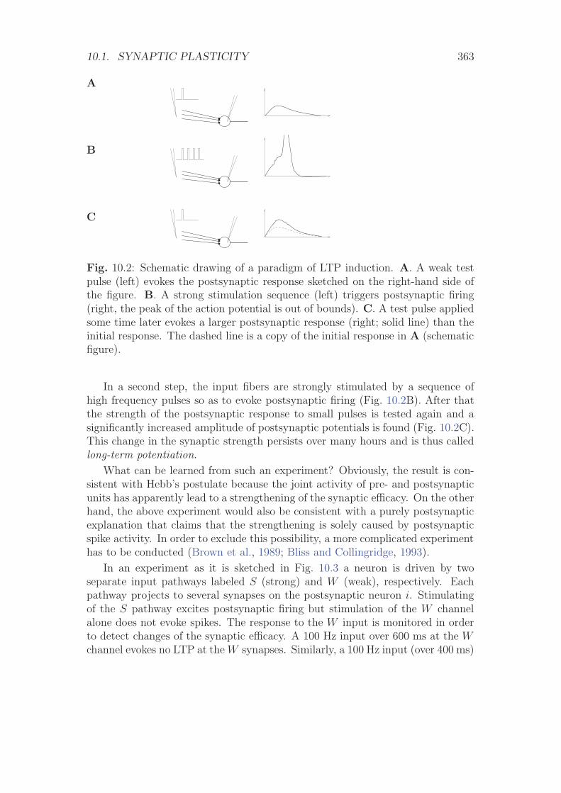
10.1. SYNAPTIC PLASTICITY 363
A
B
C
Fig. 10.2: Schematic drawing of a paradigm of LTP induction. A. A weak testpulse (left) evokes the postsynaptic response sketched on the right-hand side ofthe figure. B. A strong stimulation sequence (left) triggers postsynaptic firing(right, the peak of the action potential is out of bounds). C. A test pulse appliedsome time later evokes a larger postsynaptic response (right; solid line) than theinitial response. The dashed line is a copy of the initial response in A (schematicfigure).
In a second step, the input fibers are strongly stimulated by a sequence ofhigh frequency pulses so as to evoke postsynaptic firing (Fig. 10.2B). After thatthe strength of the postsynaptic response to small pulses is tested again and asignificantly increased amplitude of postsynaptic potentials is found (Fig. 10.2C).This change in the synaptic strength persists over many hours and is thus calledlong-term potentiation.
What can be learned from such an experiment? Obviously, the result is con-sistent with Hebb’s postulate because the joint activity of pre- and postsynapticunits has apparently lead to a strengthening of the synaptic efficacy. On the otherhand, the above experiment would also be consistent with a purely postsynapticexplanation that claims that the strengthening is solely caused by postsynapticspike activity. In order to exclude this possibility, a more complicated experimenthas to be conducted (Brown et al., 1989; Bliss and Collingridge, 1993).
In an experiment as it is sketched in Fig. 10.3 a neuron is driven by twoseparate input pathways labeled S (strong) and W (weak), respectively. Eachpathway projects to several synapses on the postsynaptic neuron i. Stimulatingof the S pathway excites postsynaptic firing but stimulation of the W channelalone does not evoke spikes. The response to the W input is monitored in orderto detect changes of the synaptic efficacy. A 100 Hz input over 600 ms at the Wchannel evokes no LTP at the W synapses. Similarly, a 100 Hz input (over 400 ms)
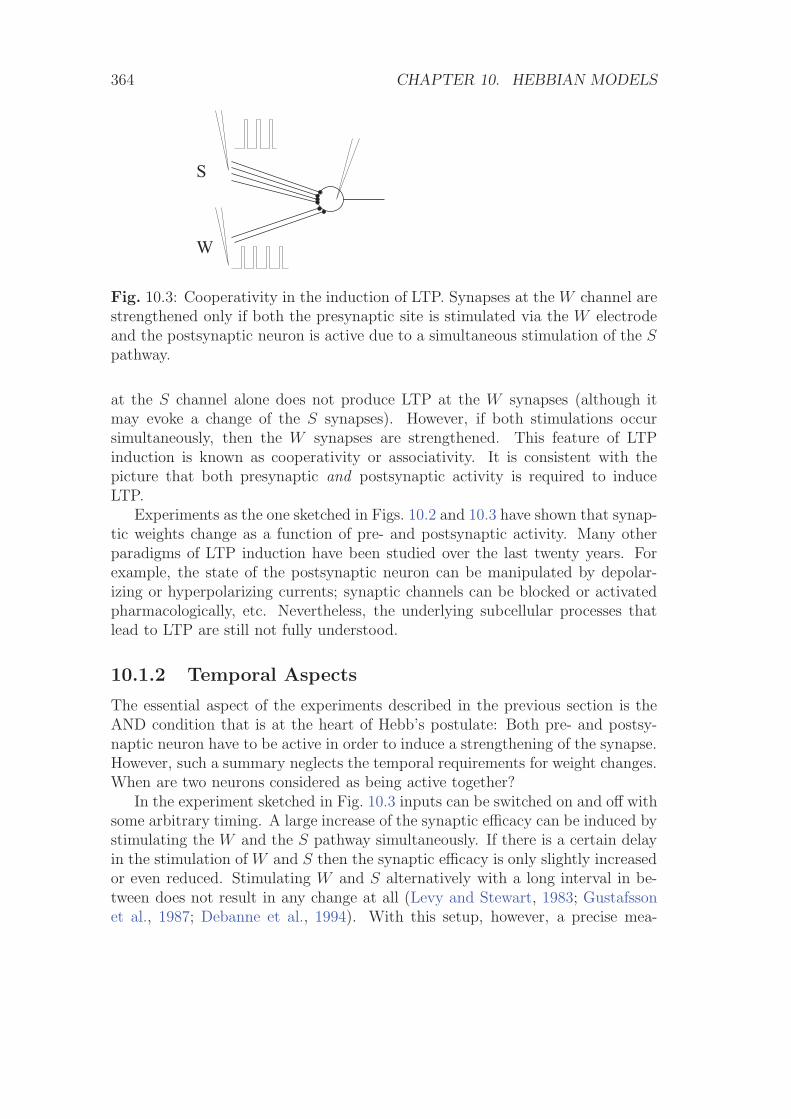
364 CHAPTER 10. HEBBIAN MODELS
S
W
Fig. 10.3: Cooperativity in the induction of LTP. Synapses at the W channel arestrengthened only if both the presynaptic site is stimulated via the W electrodeand the postsynaptic neuron is active due to a simultaneous stimulation of the Spathway.
at the S channel alone does not produce LTP at the W synapses (although itmay evoke a change of the S synapses). However, if both stimulations occursimultaneously, then the W synapses are strengthened. This feature of LTPinduction is known as cooperativity or associativity. It is consistent with thepicture that both presynaptic and postsynaptic activity is required to induceLTP.
Experiments as the one sketched in Figs. 10.2 and 10.3 have shown that synap-tic weights change as a function of pre- and postsynaptic activity. Many otherparadigms of LTP induction have been studied over the last twenty years. Forexample, the state of the postsynaptic neuron can be manipulated by depolar-izing or hyperpolarizing currents; synaptic channels can be blocked or activatedpharmacologically, etc. Nevertheless, the underlying subcellular processes thatlead to LTP are still not fully understood.
10.1.2 Temporal Aspects
The essential aspect of the experiments described in the previous section is theAND condition that is at the heart of Hebb’s postulate: Both pre- and postsy-naptic neuron have to be active in order to induce a strengthening of the synapse.However, such a summary neglects the temporal requirements for weight changes.When are two neurons considered as being active together?
In the experiment sketched in Fig. 10.3 inputs can be switched on and off withsome arbitrary timing. A large increase of the synaptic efficacy can be induced bystimulating the W and the S pathway simultaneously. If there is a certain delayin the stimulation of W and S then the synaptic efficacy is only slightly increasedor even reduced. Stimulating W and S alternatively with a long interval in be-tween does not result in any change at all (Levy and Stewart, 1983; Gustafssonet al., 1987; Debanne et al., 1994). With this setup, however, a precise mea-
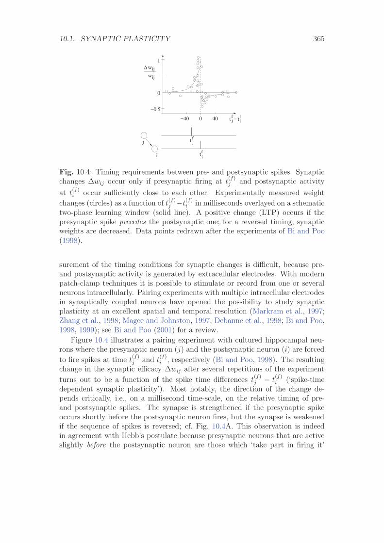
10.1. SYNAPTIC PLASTICITY 365
t jf
tfi
t jf
Δ wwij
ij
0
1
−0.5
0 40−40
j
i
− tfi
Fig. 10.4: Timing requirements between pre- and postsynaptic spikes. Synapticchanges Δwij occur only if presynaptic firing at t
(f)j and postsynaptic activity
at t(f)i occur sufficiently close to each other. Experimentally measured weight
changes (circles) as a function of t(f)j −t
(f)i in milliseconds overlayed on a schematic
two-phase learning window (solid line). A positive change (LTP) occurs if thepresynaptic spike precedes the postsynaptic one; for a reversed timing, synapticweights are decreased. Data points redrawn after the experiments of Bi and Poo(1998).
surement of the timing conditions for synaptic changes is difficult, because pre-and postsynaptic activity is generated by extracellular electrodes. With modernpatch-clamp techniques it is possible to stimulate or record from one or severalneurons intracellularly. Pairing experiments with multiple intracellular electrodesin synaptically coupled neurons have opened the possibility to study synapticplasticity at an excellent spatial and temporal resolution (Markram et al., 1997;Zhang et al., 1998; Magee and Johnston, 1997; Debanne et al., 1998; Bi and Poo,1998, 1999); see Bi and Poo (2001) for a review.
Figure 10.4 illustrates a pairing experiment with cultured hippocampal neu-rons where the presynaptic neuron (j) and the postsynaptic neuron (i) are forced
to fire spikes at time t(f)j and t
(f)i , respectively (Bi and Poo, 1998). The resulting
change in the synaptic efficacy Δwij after several repetitions of the experiment
turns out to be a function of the spike time differences t(f)j − t
(f)i (‘spike-time
dependent synaptic plasticity’). Most notably, the direction of the change de-pends critically, i.e., on a millisecond time-scale, on the relative timing of pre-and postsynaptic spikes. The synapse is strengthened if the presynaptic spikeoccurs shortly before the postsynaptic neuron fires, but the synapse is weakenedif the sequence of spikes is reversed; cf. Fig. 10.4A. This observation is indeedin agreement with Hebb’s postulate because presynaptic neurons that are activeslightly before the postsynaptic neuron are those which ‘take part in firing it’
366 CHAPTER 10. HEBBIAN MODELS
whereas those that fire later obviously did not contribute to the postsynapticaction potential. An asymmetric learning window such as the one in Fig. 10.4,is thus an implementation of the causality requirement that is implicit in Hebb’sprinciple.
Similar results on spike-time dependent synaptic plasticity have been foundin various neuronal systems (Markram et al., 1997; Zhang et al., 1998; Debanneet al., 1998; Bi and Poo, 1998, 1999; Egger et al., 1999), but there are alsocharacteristic differences. Synapses between parallel fibers and ‘Purkinje-cells’in the cerebellar-like structure of electric fish, for example, show the oppositedependence on the relative timing of presynaptic input and the (so-called ‘broad’)postsynaptic spike. In this case the synapse is weakened if the presynaptic inputarrives shortly before the postsynaptic spike (anti-Hebbian plasticity). If thetiming is the other way round then the synapse is strengthened. A change in thetiming of less than 10 ms can change the effect from depression to potentiation(Bell et al., 1997b).
10.2 Rate-Based Hebbian Learning
In order to prepare the ground for a thorough analysis of spike-based learningrules in Section 10.3 we will first review the basic concepts of correlation-basedlearning in a firing rate formalism.
10.2.1 A Mathematical Formulation of Hebb’s Rule
In order to find a mathematically formulated learning rule based on Hebb’s pos-tulate we focus on a single synapse with efficacy wij that transmits signals from apresynaptic neuron j to a postsynaptic neuron i. For the time being we contentourselves with a description in terms of mean firing rates. In the following, theactivity of the presynaptic neuron is denoted by νj and that of the postsynapticneuron by νi.
There are two aspects in Hebb’s postulate that are particularly important,viz. locality and cooperativity. Locality means that the change of the synapticefficacy can only depend on local variables, i.e., on information that is available atthe site of the synapse, such as pre- and postsynaptic firing rate, and the actualvalue of the synaptic efficacy, but not on the activity of other neurons. Basedon the locality of Hebbian plasticity we can make a rather general ansatz for thechange of the synaptic efficacy,
d
dtwij = F (wij; νi, νj) . (10.1)
Here, dwij/dt is the rate of change of the synaptic coupling strength and F is aso far undetermined function (Brown et al., 1991; Sejnowski and Tesauro, 1989;
10.2. RATE-BASED HEBBIAN LEARNING 367
Kohonen, 1984). We may wonder whether there are other local variables (e.g.,the membrane potential ui) that should be included as additional arguments ofthe function F . It turns out that in standard rate models this is not necessary,since the membrane potential ui is uniquely determined by the postsynaptic firingrate, νi = g(ui), with a monotone gain function g.
The second important aspect of Hebb’s postulate, cooperativity, implies thatpre- and postsynaptic neuron have to be active simultaneously for a synapticweight change to occur. We can use this property to learn something about thefunction F . If F is sufficiently well-behaved, we can expand F in a Taylor seriesabout νi = νj = 0,
d
dtwij = c0(wij) + cpost
1 (wij)νi + cpre1 (wij) νj
+ cpre2 (wij) ν2
j + cpost2 (wij) ν2
i + ccorr2 (wij) νi νj +O(ν3) . (10.2)
The term containing ccorr2 on the right-hand side of (10.2) is bilinear in pre- and
postsynaptic activity. This term implements the AND condition for cooperativitywhich makes Hebbian learning a useful concept.
The simplest choice for our function F is to fix ccorr2 at a positive constant and
to set all other terms in the Taylor expansion to zero. The result is the prototypeof Hebbian learning,
d
dtwij = ccorr
2 νi νj . (10.3)
We note in passing that a learning rule with ccorr2 < 0 is usually called anti-
Hebbian because it weakens the synapse if pre- and postsynaptic neuron areactive simultaneously; a behavior that is just contrary to that postulated byHebb. A learning rule with only first-order terms gives rise to so-called non-Hebbian plasticity, because pre- or postsynaptic activity alone induces a changeof the synaptic efficacy. More complicated learning rules can be constructed ifhigher-order terms in the expansion of Eq. (10.2), such as νi ν
2j , ν2
i νj , ν2i ν2
j , etc.,are included.
The dependence of F on the synaptic efficacy wij is a natural consequenceof the fact that wij is bounded. If F was independent of wij then the synapticefficacy would grow without limit if the same potentiating stimulus is applied overand over again. A saturation of synaptic weights can be achieved, for example,if the parameter ccorr
2 in Eq. (10.2) tends to zero as wij approaches its maximumvalue, say wmax = 1, e.g.,
ccorr2 (wij) = γ2 (1− wij) (10.4)
with a positive constant γ2.Hebb’s original proposal does not contain a rule for a decrease of synaptic
weights. In a system where synapses can only be strengthened, all efficacies
368 CHAPTER 10. HEBBIAN MODELS
will finally saturate at their upper maximum value. An option of decreasing theweights (synaptic depression) is therefore a necessary requirement for any usefullearning rule. This can, for example, be achieved by weight decay, which can beimplemented in Eq. (10.2) by setting
c0(wij) = −γ0 wij . (10.5)
Here, γ0 is (small) positive constant that describes the rate by which wij decaysback to zero in the absence of stimulation. Our formulation (10.2) is hence suffi-ciently general to allow for a combination of synaptic potentiation and depression.If we combine Eq. (10.4) and Eq. (10.5) we obtain the learning rule
d
dtwij = γ2 (1− wij) νi νj − γ0 wij . (10.6)
The factors (1− wij) and wij that lead to a saturation at wij = 1 for continuedstimulation and an exponential decay to wij = 0 in the absence of stimulation, re-spectively, are one possibility to implement ‘soft’ bounds for the synaptic weight.In simulations, ‘hard’ bounds are often used to restrict the synaptic weights toa finite interval, i.e., a learning rule with weight-independent parameters is onlyapplied as long as the weight stays within its limits.
Another interesting aspect of learning rules is competition. The idea is thatsynaptic weights can only grow at the expense of others so that if a certain sub-group of synapses is strengthened, other synapses to the same postsynaptic neuronhave to be weakened. Competition is essential for any form of self-organizationand pattern formation. Practically, competition can be implemented in simula-tions by normalizing the sum of all weights converging onto the same postsynapticneuron (Miller and MacKay, 1994); cf. Section 11.1.3. Though this can be moti-vated by a limitation of common synaptic resources such a learning rule violateslocality of synaptic plasticity. On the other hand, competition of synaptic weightchanges can also be achieved with purely local learning rules (Oja, 1982; Kistlerand van Hemmen, 2000a; Song et al., 2000; Kempter et al., 2001).
Example: Postsynaptic gating versus presynaptic gating
Equation (10.6) is just one possibility to specify rules for the growth and de-cay of synaptic weights. In the framework of Eq. (10.2), other formulations areconceivable; cf. Table 10.1. For example, we can define a learning rule of the form
d
dtwij = γ νi [νj − νθ(wij)] , (10.7)
where γ is a positive constant and νθ is some reference value that may depend onthe current value of wij . A weight change occurs only if the postsynaptic neuron isactive, νi > 0. We say that weight changes are ‘gated’ by the postsynaptic neuron.
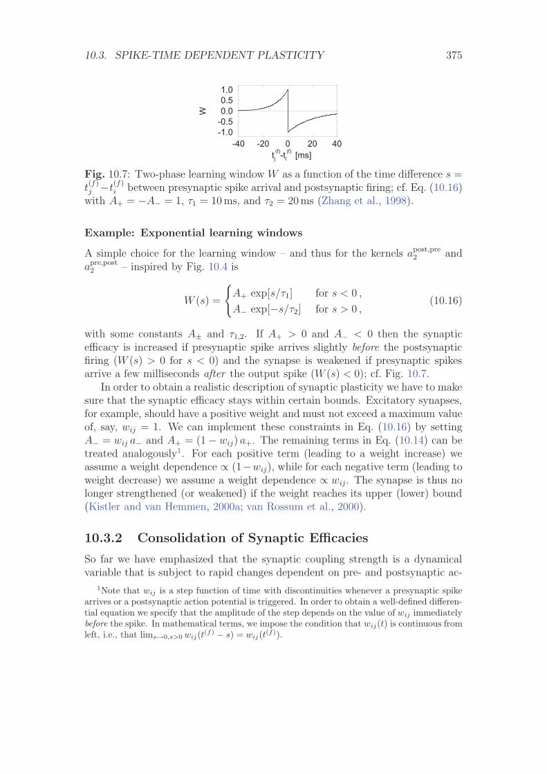
10.3. SPIKE-TIME DEPENDENT PLASTICITY 375
-40 -20 0 20 40 tj
(f)-ti(f) [ms]
-1.0-0.50.00.51.0
W
Fig. 10.7: Two-phase learning window W as a function of the time difference s =t(f)j −t
(f)i between presynaptic spike arrival and postsynaptic firing; cf. Eq. (10.16)
with A+ = −A− = 1, τ1 = 10 ms, and τ2 = 20ms (Zhang et al., 1998).
Example: Exponential learning windows
A simple choice for the learning window – and thus for the kernels apost,pre2 and
apre,post2 – inspired by Fig. 10.4 is
W (s) =
{A+ exp[s/τ1] for s < 0 ,
A− exp[−s/τ2] for s > 0 ,(10.16)
with some constants A± and τ1,2. If A+ > 0 and A− < 0 then the synapticefficacy is increased if presynaptic spike arrives slightly before the postsynapticfiring (W (s) > 0 for s < 0) and the synapse is weakened if presynaptic spikesarrive a few milliseconds after the output spike (W (s) < 0); cf. Fig. 10.7.
In order to obtain a realistic description of synaptic plasticity we have to makesure that the synaptic efficacy stays within certain bounds. Excitatory synapses,for example, should have a positive weight and must not exceed a maximum valueof, say, wij = 1. We can implement these constraints in Eq. (10.16) by settingA− = wij a− and A+ = (1− wij) a+. The remaining terms in Eq. (10.14) can betreated analogously1. For each positive term (leading to a weight increase) weassume a weight dependence ∝ (1−wij), while for each negative term (leading toweight decrease) we assume a weight dependence ∝ wij. The synapse is thus nolonger strengthened (or weakened) if the weight reaches its upper (lower) bound(Kistler and van Hemmen, 2000a; van Rossum et al., 2000).
10.3.2 Consolidation of Synaptic Efficacies
So far we have emphasized that the synaptic coupling strength is a dynamicalvariable that is subject to rapid changes dependent on pre- and postsynaptic ac-
1Note that wij is a step function of time with discontinuities whenever a presynaptic spikearrives or a postsynaptic action potential is triggered. In order to obtain a well-defined differen-tial equation we specify that the amplitude of the step depends on the value of wij immediatelybefore the spike. In mathematical terms, we impose the condition that wij(t) is continuous fromleft, i.e., that lims→0,s>0 wij(t(f) − s) = wij(t(f)).
376 CHAPTER 10. HEBBIAN MODELS
tivity. On the other hand, it is generally accepted that long-lasting modificationsof the synaptic efficacy form the basis of learning and memory. How can fastdynamical properties be reconciled with long-lasting modifications?
Most learning theories dealing with artificial neural networks concentrate onthe induction of weight changes. As soon as the ‘learning session’ is over, synapticplasticity is ‘switched off’ and weights are taken as fixed parameters. In biologicalsystems, a similar mechanism can be observed during development. There arecritical periods in the early life time of an animal where certain synapses showa form of plasticity that is ‘switched off’ after maturation (Crepel, 1982). Themajority of synapses, especially those involved in higher brain functions, however,keep their plasticity throughout their life. At first glance there is thus the risk thatpreviously stored information is simply overwritten by new input (‘palimpsestproperty’). Grossberg has coined the term ‘stability-plasticity dilemma’ for thisproblem (Grossberg, 1987; Carpenter and Grossberg, 1987).
To address these questions, Fusi et al. (2000) have studied the problem of theconsolidation of synaptic weights. They argue that bistability of synaptic weightscan solve the stability-plasticity dilemma. More specifically, the dynamics ofsynaptic efficacies is characterized by two stable fixed points at wij = 0 and wij =1. In the absence of stimulation the synaptic weight will thus settle down at eitherone of these values. Pre- or postsynaptic activity can lead to a transition fromone fixed point to the other, but only if the duration of the stimulus presentationor its amplitude exceeds a certain threshold. In other words, synapses can beswitched on or off but this will happen only for those synapses where the learningthreshold is exceeded. Learning thus affects only a few synapses so that previouslystored information is mostly preserved.
In the framework of Eq. (10.14), such a dynamics for synaptic weights can beimplemented by setting
a0(wij) = −γ wij (1− wij) (wθ − wij) , (10.17)
where 0 < wθ < 1 and γ > 0. In the absence of stimulation, small weights(wij < wθ) decay to zero whereas large weights (wij > wθ) increase towards one.Spike activity thus has to drive the synaptic weight across the threshold wθ beforelong-lasting changes take place. A combination of Eqs. (10.17) and (10.14) cantherefore be considered as a model of induction and consolidation of synapticplasticity.
10.3.3 General Framework (*)
In Eq. (10.14) weight changes occur instantaneously at the moment of presynapticspike arrival or postsynaptic firing. In this subsection we will develop a slightlymore general equation for the evolution of synaptic weights. The approach taken
10.3. SPIKE-TIME DEPENDENT PLASTICITY 377
in this section can be seen as a generalization of the Taylor expansion in the ratemodel of Section 10.2 to the case of spiking neurons.
We recall that we started our formulation of rate-based Hebbian learning froma general formula
d
dtwij = F (wij; νi, νj) (10.18)
where weight changes are given as a function of the weight wij as well as of thepre- and postsynaptic rates νj , νi; cf. Eq. (10.1). The essential assumption wasthat neuronal activity is characterized by firing rates that change slowly enough tobe considered as stationary. Hebbian rules followed then from a Taylor expansionof Eq. (10.18). In the following, we keep the idea of an expansion, but drop thesimplifications that are inherent to a description in terms of a mean firing rate.
The internal state of spiking neurons (e.g., integrate-and-fire or Spike Re-sponse Model neurons) is characterized by the membrane potential u which inturn depends on the input and the last output spike. The generalization ofEq. (10.18) to the case of spiking neurons is therefore
d
dtwij(t) = F
(wij(t); {upost
i (t′ < t)}, {uprej (t′′ < t)}) , (10.19)
where F is now a functional of the time course of pre- and postsynaptic membranepotential at the location of the synapse. Our notation with t′ and t′′ is intendedto indicate that the weight changes do not only depend on the momentary valueof the pre- and postsynaptic potential, but also on their history t′ < t and t′′ < t.The weight value wij and the local value of pre- and postsynaptic membranepotential are the essential variables that are available at the site of the synapseto control the up- and down-regulation of synaptic weights. In detailed neuronmodels, F would depend not only on the weight wij and membrane potentials,but also on all other variables that are locally available at the site of the synapse.In particular, there could be a dependence upon the local calcium concentration;cf. Section 10.4.
In analogy to the approach taken in Section 10.2, we now expand the right-hand side of Eq. (10.19) about the resting state upost
i = uprej = urest in a Volterra
series (Volterra, 1959; Palm and Poggio, 1977; van Hemmen et al., 2000). For thesake of simplicity we shift the voltage scale so that urest = 0. We find
dwij
dt= a0(wij) +
∫ ∞
0
αpre1 (wij ; s) upre
j (t− s) ds
+
∫ ∞
0
αpost1 (wij ; s
′) uposti (t− s′) ds′ (10.20)
+
∫ ∞
0
∫ ∞
0
αcorr2 (wij ; s, s
′) uprej (t− s) upost
i (t− s′) ds′ ds + . . . .
The next terms would be quadratic in uposti or upre
j and have been neglected.Equation (10.20) provides a framework for the formulation of spike-based learning
378 CHAPTER 10. HEBBIAN MODELS
rules and may be seen as the generalization of the general rate-based model thatwe have derived in Section 10.2.
In order to establish a connection with various other formulations of spike-based learning rules, we consider the time course of the pre- and postsynapticmembrane potential in more detail. At the presynaptic terminal, the membranepotential is most of the time at rest, except when an action potential arrives.Since the duration of each action potential is short, the presynaptic membranepotential can be approximated by a train of δ functions
uprej (t) =
∑f
δ(t− t(f)j ) (10.21)
where t(f)j denotes the spike arrival times at the presynaptic terminal.
The situation at the postsynaptic site is somewhat more complicated. For thesimple spike response model SRM0, the membrane potential can be written as
uposti (t) = η(t− ti) + hi(t) , (10.22)
where ti is the last postsynaptic firing time. In contrast to the usual interpretationof terms on the right-hand side of Eq. (10.22), the function η is now taken as thetime course of the back propagating action potential at the location of the synapse.Similarly, hi(t) is the local postsynaptic potential at the synapse.
For a further simplification of Eq. (10.20), we need to make some approxi-mations. Specifically we will explore two different approximation schemes. Inthe first scheme, we suppose that the dominating term on the right-hand side ofEq. (10.22) is the back propagating action potential, while in the second schemewe neglect η and consider h as the dominant term. Let us discuss both approxi-mations in turn.
(i) Sharply peaked back propagating action potential
We assume that the back propagating action potential is sharply peaked, i.e., ithas a large amplitude and short duration. In this case, the membrane potentialof the postsynaptic neuron is dominated by the back propagating action poten-tial and the term h(t) in Eq. (10.22) can be neglected. Furthermore η can beapproximated by a δ function. The membrane potential at the postsynaptic sitereduces then to a train of pulses,
uposti (t) =
∑f
δ(t− t(f)i ) , (10.23)
where t(f)i denotes the postsynaptic firing times. Equation (10.23) is a sensible
approximation for synapses that are located on or close to the soma so that thefull somatic action potential is ‘felt’ by the postsynaptic neuron. For neurons with
10.3. SPIKE-TIME DEPENDENT PLASTICITY 379
active processes in the dendrite that keep the back propagating action potentialwell focused, Eq. (10.23) is also a reasonable approximation for synapses that arefurther away from the soma. A transmission delay for back propagation of thespike from the soma to the site of the synapse can be incorporated at no extracost.
If we insert Eqs. (10.21) and (10.23) into Eq. (10.20) we find
dwij
dt= a0 +
∑f
αpre1 (t− t
(f)j ) +
∑f
αpost1 (t− t
(f)i )
+∑
f
∑f
αcorr2 (t− t
(f)i , t− t
(f)j ) + . . . , (10.24)
where we have omitted the wij dependence of the right-hand side terms. Incontrast to Eq. (10.14) weight changes are now continuous. A single presynaptic
spike at time t(f)j , for example, will cause a weight change that builds up during
some time after t(f)j . An example will be given below in Eq. (10.31).
In typical plasticity experiments, the synaptic weight is monitored every fewhundred milliseconds so that the exact time course of the functions, αpre
1 , αpost1
and αcorr2 is not measured. To establish the connection to Eq. (10.14), we now
assume that the weight changes are rapid compared to the time scale of weightmonitoring. In other words, we make the replacement
αpre1 (t− t
(f)j ) −→ apre
1 δ(t− t(f)j ) (10.25)
αpost1 (t− t
(f)i ) −→ apost
1 δ(t− t(f)i ) (10.26)
where apre1 =
∫∞0
αpre1 (s) ds and apost
1 =∫∞
0αpost
1 (s) ds . For the correlation termwe exploit the invariance with respect to time translation, i.e., the final resultonly depends on the time difference t
(f)j − t
(f)i . The weight update occurs at
the moment of the postsynaptic spike if t(f)j < t
(f)i and at the moment of the
presynaptic spike if t(f)j > t
(f)i . Hence, the assumption of instantaneous update
yields two terms
αcorr2 (t−t
(f)i , t−t
(f)j ) −→
{apre,post
2 (t(f)j − t
(f)i ) δ(t− t
(f)j ) if t
(f)i < t
(f)j
apost,pre2 (t
(f)i − t
(f)j ) δ(t− t
(f)i ) if t
(f)i > t
(f)j
(10.27)
Thus, for sharply peaked back propagating action potentials and rapid weightchanges, the general framework of Eq. (10.20) leads us back to the Eq. (10.14).
(ii) No back propagating action potential
In the second approximation scheme, we assume that the membrane potential atthe location of the synapse is dominated by the slowly varying potential hi(t).
380 CHAPTER 10. HEBBIAN MODELS
This is, for example, a valid assumption in voltage-clamp experiments where thepostsynaptic neuron is artificially kept at a constant membrane potential hpost.This is also a good approximation for synapses that are located far away fromthe soma on a passive dendrite, so that the back propagation of somatic actionpotentials is negligible.
Let us consider a voltage clamp experiment where hi(t) is kept at a constantlevel hpost. As before, we suppose that weight changes are rapid. If we insertupre
j (t) =∑
f δ(t− t(f)j ) and upost
i (t) = hpost into Eq. (10.20), we find
dwij
dt= a0 +
∑f
apre1 δ(t− t
(f)j )
+apost1 hpost + acorr
2 hpost∑
f
δ(t− t(f)j ) + . . . (10.28)
where apre1 =
∫∞0
αpre1 (s) ds, apost
1 =∫∞
0αpost
1 (s) ds and acorr2 =
∫∞0
∫∞0
acorr2 (s, s′) ds ds′.
Equation (10.28) is the starting point of the theory of spike-based learning of Fusiet al. (2000). Weight changes are triggered by presynaptic spikes. The directionand value of the weight update depends on the postsynaptic membrane poten-tial. In our framework, Eq. (10.28) is a special case of the slightly more generalEq. (10.20).
10.4 Detailed Models of Synaptic Plasticity
In the previous section we have introduced a purely phenomenological modelfor spike-time dependent synaptic plasticity which is at least qualitatively inagreement with experimental results. In this section we take a slightly differentapproach and discuss how the core idea of this model, the learning window,arises from elementary kinetic processes. We start in Section 10.4.1 with a simplemechanistic model and turn then, in Section 10.4.2 to a more detailed modelwith saturation. A calcium-based model is the topic of Section 10.4.3. All threemodels give a qualitative explanation for the learning dynamics on the level ofindividual spikes.
10.4.1 A Simple Mechanistic Model
The AND condition in Hebb’s postulate suggests that two biochemical compo-nents are involved in the induction of LTP. We do not wish to speculate on thenature of these components, but simply call them a and b. We assume that thefirst component is generated by a chemical reaction chain triggered by presynap-tic spike arrival. In the absence of further input, the concentration [a] decayswith a time constant τa back to its resting level [a] = 0. A simple way to describe
10.4. DETAILED MODELS OF SYNAPTIC PLASTICITY 381
this process isd
dt[a] = − [a]
τa+ da
∑f
δ(t− t(f)j ) , (10.29)
where the sum runs over all presynaptic firing times t(f)j . Equation (10.29) states
that [a] is increased at each arrival of a presynaptic spike by an amount da. Ahigh level of [a] sets the synapse in a state where it is susceptible to changes in itsweight. The variable [a] by itself, however, does not yet trigger a weight change.
To generate the synaptic change, another substance b is needed. The produc-tion of b is controlled by a second process triggered by postsynaptic spikes,
d
dt[b] = − [b]
τb
+ db
∑f
δ(t− t(f)i ) , (10.30)
where τb is another time constant. The sum runs over all postsynaptic spikes t(f)i .
Note that the second variable [b] does not need to be a biochemical quantity; itcould, for example, be the electrical potential caused by the postsynaptic spikeitself.
Hebbian learning needs both ‘substances’ to be present at the same time, thus
d
dtwcorr
ij = γ [a(t)] [b(t)] , (10.31)
with some rate constant γ. The upper index corr is intended to remind us thatwe are dealing only with the correlation term on the right-hand side of Eq. (10.14)or Eq. (10.24).
Let us now consider the synaptic change caused by a single presynaptic spikeat t
(f)j ≥ 0 and a postsynaptic spike a t
(f)i = t
(f)j − s. Integration of Eqs. (10.29)
and (10.30) yields
[a(t)] = da exp[−(t− t(f)j )/τa] Θ(t− t
(f)j )
[b(t)] = db exp[−(t− t(f)i )/τb] Θ(t− t
(f)i ) , (10.32)
where Θ(.) denotes the Heaviside step function as usual. The change caused by
the pair of pulses (t(f)i , t
(f)j ), measured after a time T , is
∫ T
0
(d
dtwcorr
ij
)dt = γ da db
∫ T
max{t(f)j ,t
(f)i }
exp
[−t− t
(f)j
τa− t− t
(f)i
τb
]dt . (10.33)
The integral over t can be calculated explicitely. The total weight change that isobtained for T � τa, τb can be identified with the learning window. Thus we find
W (s) =
{A exp[s/τa] for s < 0
A exp[−s/τb] for s > 0(10.34)
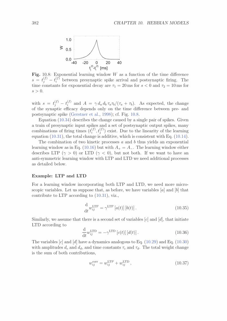
382 CHAPTER 10. HEBBIAN MODELS
-40 -20 0 20 40 tj
(f)-ti(f) [ms]
0.0
0.5
1.0
W
Fig. 10.8: Exponential learning window W as a function of the time differences = t
(f)j − t
(f)i between presynaptic spike arrival and postsynaptic firing. The
time constants for exponential decay are τ1 = 20ms for s < 0 and τ2 = 10ms fors > 0.
with s = t(f)j − t
(f)i and A = γ da db τaτb/(τa + τb). As expected, the change
of the synaptic efficacy depends only on the time difference between pre- andpostsynaptic spike (Gerstner et al., 1998); cf. Fig. 10.8.
Equation (10.34) describes the change caused by a single pair of spikes. Givena train of presynaptic input spikes and a set of postsynaptic output spikes, manycombinations of firing times (t
(f)i , t
(f)j ) exist. Due to the linearity of the learning
equation (10.31), the total change is additive, which is consistent with Eq. (10.14).The combination of two kinetic processes a and b thus yields an exponential
learning window as in Eq. (10.16) but with A+ = A−. The learning window eitherdescribes LTP (γ > 0) or LTD (γ < 0), but not both. If we want to have ananti-symmetric learning window with LTP and LTD we need additional processesas detailed below.
Example: LTP and LTD
For a learning window incorporating both LTP and LTD, we need more micro-scopic variables. Let us suppose that, as before, we have variables [a] and [b] thatcontribute to LTP according to (10.31), viz.,
d
dtwLTP
ij = γLTP [a(t)] [b(t)] . (10.35)
Similarly, we assume that there is a second set of variables [c] and [d], that initiateLTD according to
d
dtwLTD
ij = −γLTD [c(t)] [d(t)] . (10.36)
The variables [c] and [d] have a dynamics analogous to Eq. (10.29) and Eq. (10.30)with amplitudes dc and dd, and time constants τc and τd. The total weight changeis the sum of both contributions,
wcorrij = wLTP
ij + wLTDij , (10.37)
10.4. DETAILED MODELS OF SYNAPTIC PLASTICITY 383
and so is the learning window, i.e.,
W (s) =
{A+ exp[s/τa]−A− exp[s/τc] for s < 0
A+ exp[−s/τb]− A− exp[−s/τd] for s > 0(10.38)
with A+ = γLTP da db τaτb/(τa + τb) and A− = γLTD dc dd τcτd/(τc + τd) (Gerstneret al., 1996a, 1998).
We now set db = 1/τb and dc = 1/τc. In the limit of τb → 0 and τc → 0,we find the asymmetric two-phase learning window introduced in Eq. (10.16).Weight changes are now instantaneous. A postsynaptic spike that is triggeredafter a presynaptic spike arrival reads out the current value of [a] and inducesLTP by an amount
W (t(f)j − t
(f)i ) = γLTP da exp
(−t
(f)i − t
(f)j
τa
)for t
(f)j < t
(f)i . (10.39)
A presynaptic spike t(f)j that arrives after a postsynaptic spike reads out the
current value of [d] and induces LTD by an amount
W (t(f)j − t
(f)i ) = −γ LTDdd exp
(−t
(f)j − t
(f)i
τd
)for t
(f)j > t
(f)i . (10.40)
10.4.2 A Kinetic Model based on NMDA Receptors
A model for LTP and LTD that is slightly more elaborate than the simplisticmodel discussed in the previous section has been developed by Senn et al. (1997,2001b). This model is based on the assumption that NMDA receptors can be inone of three different states, a resting state, an ‘up’ and a ‘down’ state. Tran-sitions between these states are triggered by presynaptic spike arrival (‘rest’→‘up’) and postsynaptic firing (‘rest’→ ‘down’). The actual induction of LTP orLTD, however, requires another step, namely the activation of so-called second-messengers. The model assumes two types of second-messenger, one for LTP andone for LTD. If a presynaptic spike arrives before a postsynaptic spike, the up-regulation of the NMDA receptors in combination with the activitation S1 → Sup
of the first second-messenger triggers synaptic changes that lead to LTP. On theother hand, if the presynaptic spike arrives after postsynaptic firing, the NMDAreceptors are downregulated and the activation S2 → Sdn of the other second-messenger triggers LTD; cf. Fig. 10.9
The variables Nup, Ndn, and N rest describe the portion of NMDA receptorsthat are in one of the three possible states (Nup+Ndn+N rest = 1). In the absenceof pre- and postsynaptic spikes, all receptors return to the rest state,
d
dtN rest =
Nup
τNup
+Ndn
τNdn
. (10.41)
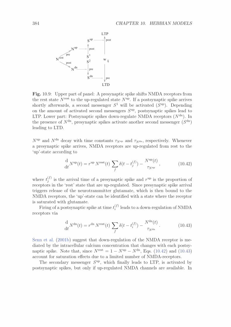
384 CHAPTER 10. HEBBIAN MODELS
N
N
N
S
LTP
LTD
S
S
up
up
dn
dn
2
1Sij
post
pre
post
pre
wrest
post
pre
Fig. 10.9: Upper part of panel: A presynaptic spike shifts NMDA receptors fromthe rest state N rest to the up-regulated state Nup. If a postsynaptic spike arrivesshortly afterwards, a second messenger S1 will be activated (Sup). Dependingon the amount of activated second messengers Sup, postsynaptic spikes lead toLTP. Lower part: Postsynaptic spikes down-regulate NMDA receptors (N dn). Inthe presence of Ndn, presynaptic spikes activate another second messenger (Sdn)leading to LTD.
Nup and Ndn decay with time constants τNup and τNdn , respectively. Whenevera presynaptic spike arrives, NMDA receptors are up-regulated from rest to the‘up’-state according to
d
dtNup(t) = rup N rest(t)
∑f
δ(t− t(f)j )− Nup(t)
τNup
, (10.42)
where t(f)j is the arrival time of a presynaptic spike and rup is the proportion of
receptors in the ‘rest’ state that are up-regulated. Since presynaptic spike arrivaltriggers release of the neurotransmitter glutamate, which is then bound to theNMDA receptors, the ‘up’-state can be identified with a state where the receptoris saturated with glutamate.
Firing of a postsynaptic spike at time t(f)i leads to a down-regulation of NMDA
receptors via
d
dtNdn(t) = rdn N rest(t)
∑f
δ(t− t(f)i )− Ndn(t)
τNdn
. (10.43)
Senn et al. (2001b) suggest that down-regulation of the NMDA receptor is me-diated by the intracellular calcium concentration that changes with each postsy-naptic spike. Note that, since N rest = 1 − Nup − Ndn, Eqs. (10.42) and (10.43)account for saturation effects due to a limited number of NMDA-receptors.
The secondary messenger Sup, which finally leads to LTP, is activated bypostsynaptic spikes, but only if up-regulated NMDA channels are available. In
10.4. DETAILED MODELS OF SYNAPTIC PLASTICITY 385
the absence of postsynaptic spikes the concentration of second messengers decayswith time constant τSup . Thus
d
dtSup(t) = −Sup(t)
τSup
+ rS Nup(t) [1− Sup(t)]∑
f
δ(t− t(f)i ) , (10.44)
where rS is a rate constant. Since Nup(t) > 0 requires that a presynaptic spikehas occurred before t, the activation of Sup effectively depends on the specifictiming of pre- and postsynaptic spikes (‘first pre, then post’).
Similarly, the other second messenger Sdn is activated by a presynaptic spikeprovided that there are receptors in their down regulated state, i.e.,
d
dtSdn(t) = −Sdn(t)
τSdn
+ rS Ndn(t) [1− Sdn(t)]∑
f
δ(t− t(f)j ) , (10.45)
where τSdn is another decay time constant. The second messenger Sdn is thereforetriggered by the sequence ‘first post, then pre’. The factors [1−Sup] in Eq. (10.44)and [1−Sdn] in Eq. (10.45) account for the limited amount of second messengersavailable at the synapse.
Long-term potentiation (weight increase) depends on the presence of Sup,long-term depression (weight decrease) on Sdn. This is described by
d
dtwij = γLTP (1− wij) [Sup − θup]+
∑f
δ(t− t(f)i −Δ)
−γLTD wij [Sdn − θd]+∑
f
δ(t− t(f)j −Δ) (10.46)
with certain parameters γLTP/D and θup/dn. Here, [x]+ = x Θ(x) denotes a piece-wise linear function with [x]+ = x for x > 0 and zero otherwise. The delay0 < Δ 1 ensures that the actual weight change occurs after the update ofSup, Sdn. Note that this is a third-order model. The variable Sup > 0, for exam-ple, is already second-order, because it depends on presynaptic spikes followedby postsynaptic action potentials. In Eq. (10.46) the postsynaptic spike is thenused again in order to trigger the weight change.
Example: Low Rates
For low pre- and postsynaptic firing rates, saturation effects can be neglected andEq. (10.46) is equivalent to the elementary model discussed in Section 10.4.1. Letus assume that a single spike induces a small change (rdn, rup 1) so that wecan use N rest ≈ 1 in Eqs. (10.42) and (10.43). The equations for Nup and Ndn
are then identical to those for the ‘substances’ [a] and [d] in Eqs. (10.29), (10.35),and (10.36).
386 CHAPTER 10. HEBBIAN MODELS
Let us furthermore assume that interspike intervals are long compared to thedecay time constants τSup , τSdn in Eqs. (10.44) and (10.45). Then Sup is negligibleexcept during and shortly after a postsynaptic action potential. At the momentof postsynaptic firing, Sup ‘reads out’ the current value of Nup; cf. Eq. (10.44). Ifthis value is large than Θup, it triggers a positive weight change; cf. Eq. (10.46).Similarly, at the moment of presynaptic spike arrival Sdn ‘reads out’ the value ofNdn and triggers a weight decrease. Thus, in this limit, the model of Senn et al.corresponds to an exponential time window
W (s) =
{A+(wij) exp[+s/τNup ] for s < 0A−(wij) exp[−s/τNdn ] for s > 0
(10.47)
with A+(wij) = rup rS (1− wij) and A−(wij) = −rdn rS wij .
Example: High Rates
If we assume that all decay time constants are much longer than typical interspikeintervals then the variables Nup/dn and Sup/dn will finally reach a steady state. Ifwe neglect correlations between pre- and postsynaptic neuron by replacing spiketrains by rates, we can solve for these stationary states,
Nup∞ =
τNup rup νj
1 + τNup rup νj + τNdnrdnνi
(10.48)
Sup∞ =
τSup rS Nup νi
1 + τSuprS Nup νi(10.49)
and similar equations for Ndn and Sdn. Note that Sup∞ is a function of νi and νj .
If we put the equations for Sup∞ and Sdn
∞ in Eq. (10.46) we get an expression ofthe form
d
dtwij = γLTP (1− wij) fLTP(νi, νj) νi − γLTD wij fLTD(νi, νj) νj (10.50)
with functions fLTP and fLTD. We linearize fLTP with respect to νj about areference value ν > 0 and evaluate fLTD at νj = ν in order to make the right-hand side of Eq. (10.50) linear in the input νj . The result is
d
dtwij = φ(wij; νi) νj (10.51)
with φ(wij; 0) = φ(wij; νθ) = 0 for some value νθ and dφ/dνi < 0 at νi = 0.Equation (10.51) is a generalized Bienenstock-Cooper-Monroe rule where φ doesnot only depend on the postsynaptic rate νi but also on the individual synapticweight; cf. Eq. (10.12). For details see Senn et al. (2001b); Bienenstock et al.(1982).
10.4. DETAILED MODELS OF SYNAPTIC PLASTICITY 387
10.4.3 A Calcium-Based Model
It has been recognized for a long time that calcium ions are an important sec-ond messenger for the induction of LTP and LTD in Hippocampus (Malenkaet al., 1988; Malinow et al., 1989; Lisman, 1989) and cerebellum (Konnerth andEilers, 1994; Lev-Ram et al., 1997). Particularly well investigated are ‘NMDAsynapses’ in the hippocampus (Collingridge et al., 1983; Dudek and Bear, 1992;Bliss and Collingridge, 1993; Bindman et al., 1991) where calcium ions can en-ter the cell through channels that are controlled by a glutamate receptor subtypecalled NMDA (N-methyl-D-aspartic acid) receptor; cf. Section 2.4.2. These chan-nels are involved in transmission of action potentials in glutamatergic (excitatory)synapses. If an action potential arrives at the presynaptic terminal, glutamate,the most common excitatory neurotransmitter, is released into the synaptic cleftand diffuses to the postsynaptic membrane where it binds to NMDA and AMPAreceptors. The binding to AMPA receptors results in the opening of the associ-ated ion channels and hence to a depolarization of the postsynaptic membrane.Channels controlled by NMDA receptors, however, are blocked by magnesiumions and do not open unless the membrane is sufficiently depolarized so as to re-move the block. Therefore, calcium ions can enter the cell only if glutamate hasbeen released by presynaptic activity and if the postsynaptic membrane is suffi-ciently depolarized. The calcium influx is the first step in a complex bio-chemicalpathway that leads ultimately to a modification of the glutamate-sensitivity ofthe postsynaptic membrane.
Biophysical models of Hebbian plasticity (Lisman, 1989; Zador et al., 1990;Holmes and Levy, 1990; Gold and Bear, 1994; Schiegg et al., 1995; Shouval et al.,2001) contain two essential components, viz. a description of intracellular cal-cium dynamics, in particular a model of calcium entry through NMDA synapses;and a hypothesis of how the concentration of intracellular calcium influences thechange of synaptic efficacy. In this section we give a simplified account of bothcomponents. We start with a model of NMDA synapses and turn then to theso-called calcium control hypothesis of Shouval et al. (2001).
NMDA receptor as a coincidence detector
We have emphasized in Sections 10.1–10.3 that all Hebbian learning rules containa term that depends on the correlation between the firings of pre- and postsy-naptic neurons. The signaling chain that leads to a weight change therefore hasto contain a nonlinear processing step that requires that pre- and postsynapticneurons are active within some short time window. Synaptic channels controlledby NMDA receptors are an excellent candidate for a biophysical implementationof this condition of ‘coincidence’ because the opening of the channel requiresboth the presence of glutamate which reflects presynaptic activity and, in orderto remove the magnesium block, a depolarization of the postsynaptic membrane
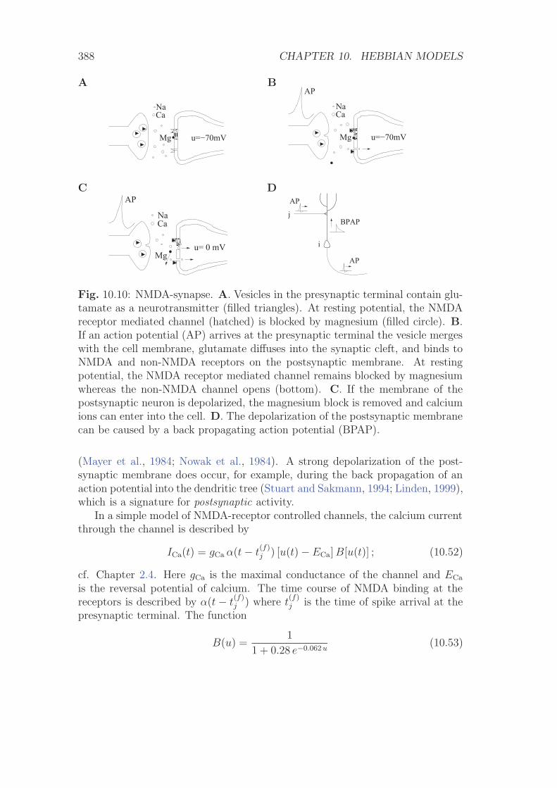
388 CHAPTER 10. HEBBIAN MODELS
A B
���������� �
���������� �
NaCa
u=−70mVMg � � �� ���� ���� ���� ���
� ���� ���� ���� ���� ���
NaCa
AP
u=−70mVMg
C D
� ���� ���� � �
� ���� ���� � �
NaCa
u= 0 mV
AP
Mg
j
i
BPAP
AP
AP
Fig. 10.10: NMDA-synapse. A. Vesicles in the presynaptic terminal contain glu-tamate as a neurotransmitter (filled triangles). At resting potential, the NMDAreceptor mediated channel (hatched) is blocked by magnesium (filled circle). B.If an action potential (AP) arrives at the presynaptic terminal the vesicle mergeswith the cell membrane, glutamate diffuses into the synaptic cleft, and binds toNMDA and non-NMDA receptors on the postsynaptic membrane. At restingpotential, the NMDA receptor mediated channel remains blocked by magnesiumwhereas the non-NMDA channel opens (bottom). C. If the membrane of thepostsynaptic neuron is depolarized, the magnesium block is removed and calciumions can enter into the cell. D. The depolarization of the postsynaptic membranecan be caused by a back propagating action potential (BPAP).
(Mayer et al., 1984; Nowak et al., 1984). A strong depolarization of the post-synaptic membrane does occur, for example, during the back propagation of anaction potential into the dendritic tree (Stuart and Sakmann, 1994; Linden, 1999),which is a signature for postsynaptic activity.
In a simple model of NMDA-receptor controlled channels, the calcium currentthrough the channel is described by
ICa(t) = gCa α(t− t(f)j ) [u(t)−ECa] B[u(t)] ; (10.52)
cf. Chapter 2.4. Here gCa is the maximal conductance of the channel and ECa
is the reversal potential of calcium. The time course of NMDA binding at thereceptors is described by α(t− t
(f)j ) where t
(f)j is the time of spike arrival at the
presynaptic terminal. The function
B(u) =1
1 + 0.28 e−0.062u(10.53)
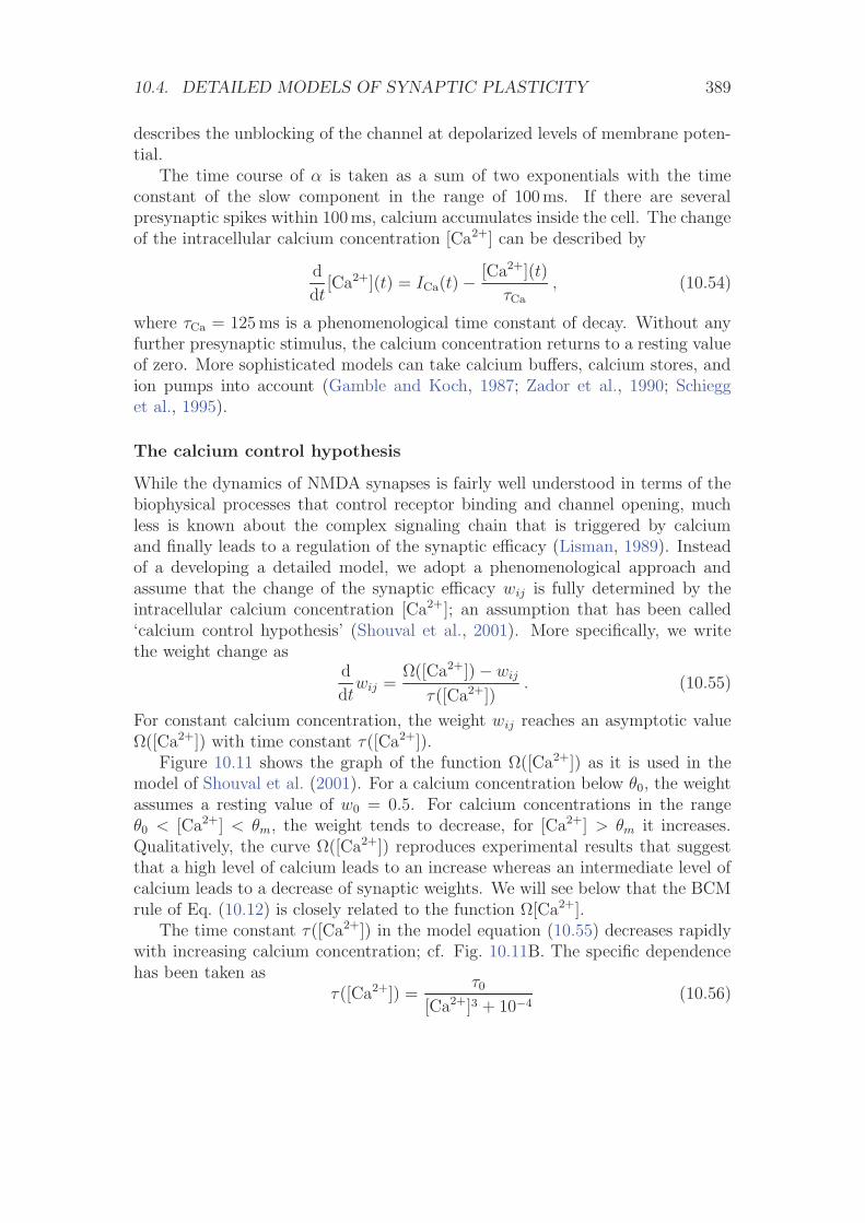
10.4. DETAILED MODELS OF SYNAPTIC PLASTICITY 389
describes the unblocking of the channel at depolarized levels of membrane poten-tial.
The time course of α is taken as a sum of two exponentials with the timeconstant of the slow component in the range of 100ms. If there are severalpresynaptic spikes within 100ms, calcium accumulates inside the cell. The changeof the intracellular calcium concentration [Ca2+] can be described by
d
dt[Ca2+](t) = ICa(t)− [Ca2+](t)
τCa
, (10.54)
where τCa = 125 ms is a phenomenological time constant of decay. Without anyfurther presynaptic stimulus, the calcium concentration returns to a resting valueof zero. More sophisticated models can take calcium buffers, calcium stores, andion pumps into account (Gamble and Koch, 1987; Zador et al., 1990; Schiegget al., 1995).
The calcium control hypothesis
While the dynamics of NMDA synapses is fairly well understood in terms of thebiophysical processes that control receptor binding and channel opening, muchless is known about the complex signaling chain that is triggered by calciumand finally leads to a regulation of the synaptic efficacy (Lisman, 1989). Insteadof a developing a detailed model, we adopt a phenomenological approach andassume that the change of the synaptic efficacy wij is fully determined by theintracellular calcium concentration [Ca2+]; an assumption that has been called‘calcium control hypothesis’ (Shouval et al., 2001). More specifically, we writethe weight change as
d
dtwij =
Ω([Ca2+])− wij
τ([Ca2+]). (10.55)
For constant calcium concentration, the weight wij reaches an asymptotic valueΩ([Ca2+]) with time constant τ([Ca2+]).
Figure 10.11 shows the graph of the function Ω([Ca2+]) as it is used in themodel of Shouval et al. (2001). For a calcium concentration below θ0, the weightassumes a resting value of w0 = 0.5. For calcium concentrations in the rangeθ0 < [Ca2+] < θm, the weight tends to decrease, for [Ca2+] > θm it increases.Qualitatively, the curve Ω([Ca2+]) reproduces experimental results that suggestthat a high level of calcium leads to an increase whereas an intermediate level ofcalcium leads to a decrease of synaptic weights. We will see below that the BCMrule of Eq. (10.12) is closely related to the function Ω[Ca2+].
The time constant τ([Ca2+]) in the model equation (10.55) decreases rapidlywith increasing calcium concentration; cf. Fig. 10.11B. The specific dependencehas been taken as
τ([Ca2+]) =τ0
[Ca2+]3 + 10−4(10.56)
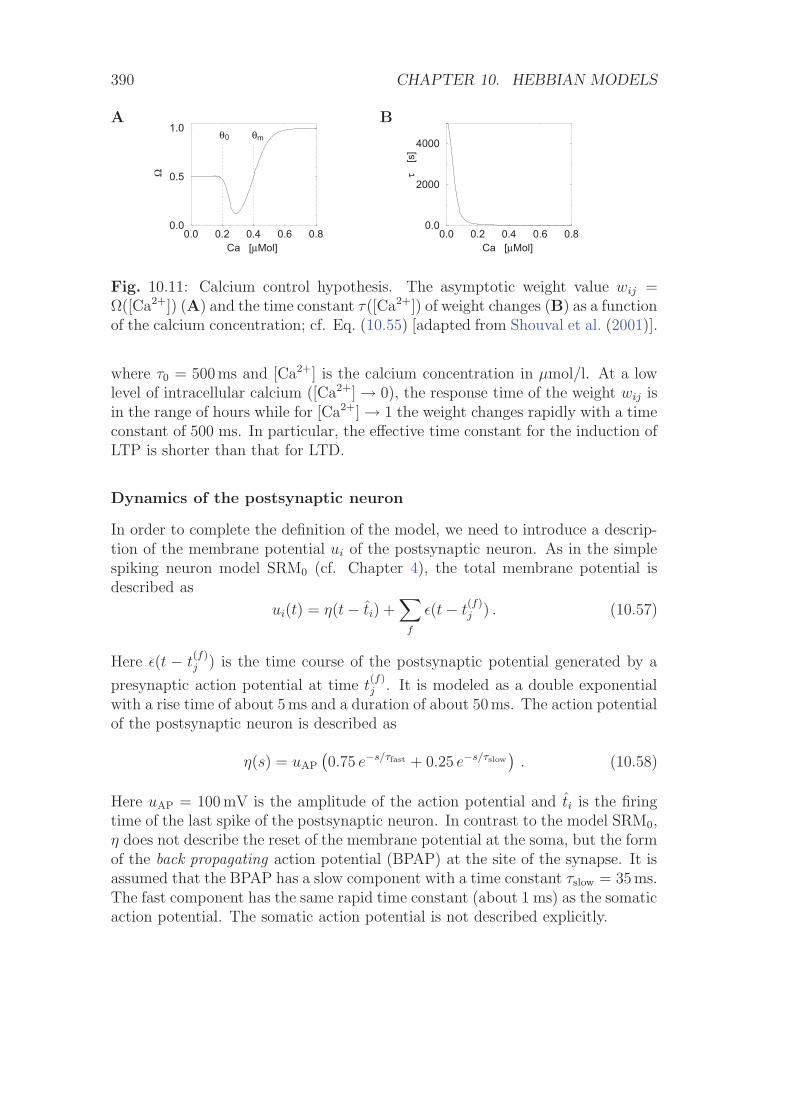
390 CHAPTER 10. HEBBIAN MODELS
A B
0.0 0.2 0.4 0.6 0.8Ca [μMol]
0.0
0.5
1.0
Ω
0 mθ θ
0.0 0.2 0.4 0.6 0.8Ca [μMol]
0.0
2000
4000
τ
[s
]
Fig. 10.11: Calcium control hypothesis. The asymptotic weight value wij =Ω([Ca2+]) (A) and the time constant τ([Ca2+]) of weight changes (B) as a functionof the calcium concentration; cf. Eq. (10.55) [adapted from Shouval et al. (2001)].
where τ0 = 500ms and [Ca2+] is the calcium concentration in μmol/l. At a lowlevel of intracellular calcium ([Ca2+]→ 0), the response time of the weight wij isin the range of hours while for [Ca2+]→ 1 the weight changes rapidly with a timeconstant of 500 ms. In particular, the effective time constant for the induction ofLTP is shorter than that for LTD.
Dynamics of the postsynaptic neuron
In order to complete the definition of the model, we need to introduce a descrip-tion of the membrane potential ui of the postsynaptic neuron. As in the simplespiking neuron model SRM0 (cf. Chapter 4), the total membrane potential isdescribed as
ui(t) = η(t− ti) +∑
f
ε(t− t(f)j ) . (10.57)
Here ε(t − t(f)j ) is the time course of the postsynaptic potential generated by a
presynaptic action potential at time t(f)j . It is modeled as a double exponential
with a rise time of about 5ms and a duration of about 50ms. The action potentialof the postsynaptic neuron is described as
η(s) = uAP
(0.75 e−s/τfast + 0.25 e−s/τslow
). (10.58)
Here uAP = 100 mV is the amplitude of the action potential and ti is the firingtime of the last spike of the postsynaptic neuron. In contrast to the model SRM0,η does not describe the reset of the membrane potential at the soma, but the formof the back propagating action potential (BPAP) at the site of the synapse. It isassumed that the BPAP has a slow component with a time constant τslow = 35ms.The fast component has the same rapid time constant (about 1 ms) as the somaticaction potential. The somatic action potential is not described explicitly.
10.4. DETAILED MODELS OF SYNAPTIC PLASTICITY 391
AC
a[
]M
olμ
0.0
0.4
0.2
t [ms]10000
m
0θ
θ
B
ft − t if
j
0−100 100
w
0.5
1.0
ij
[ms]
C1.0
0.5
wij
−80u0 [mV]
0
Fig. 10.12: Spike-time dependent plasticity in a calcium-based model. A. Cal-cium transient generated by a presynaptic spike in the absence of postsynapticfiring (bottom) and in the presence of a postsynaptic spike 10ms before (middle)or 10ms after (top) presynaptic spike arrival. Only for the sequence ‘pre-before-post’ the threshold θm for LTP can be reached. B. The final weights obtainedafter several thousands pre- and postsynaptic spikes that are generated at a rateof 1 Hz (solid line) or 3 Hz (dashed line). The weights are given as a function of
the time difference between presynaptic spikes t(f)j and postsynaptic spikes t
(f)i .
C. Pairing of presynaptic spikes with postsynaptic depolarization. The weightswij that are obtained after several hundreds of presynaptic spikes (at a rate ofνj = 0.5 Hz) as a function of the depolarization of the postsynaptic membrane.[Adapted from Shouval et al. (2001)].
Results
Given the above components of the model, we can understand intuitively howcalcium influx at NMDA synapses leads to spike-time dependent plasticity. Let usanalyze the behavior by comparing the calcium-based model with the elementarymodel of Section 10.4.1; cf. Eqs. (10.29)–(10.31). Binding of glutamate at NMDAreceptors plays the role of the component a that is triggered by presynaptic firing;the back propagating action potential plays the role of the component b that istriggered by postsynaptic firing. As a result of the depolarization caused bythe BPAP, the magnesium block is removed and calcium ions enter the cell. Thecalcium influx is proportional to the product of the NMDA-binding, i.e., the factorα in Eq. (10.52), and the unblocking, i.e., the factor B(u). Finally, the increasein the calcium concentration leads to a weight change according to Eq. (10.55).
A single presynaptic spike (without a simultaneous postsynaptic action po-tential) leads to a calcium transient that stays below the induction threshold θ0;cf. Fig. 10.12A. If a postsynaptic spike occurs 10ms before the presynaptic spikearrival, the calcium transient has a somewhat larger amplitude that attains alevel above θ0. As a consequence, the weight wij is reduced. If, however, thepostsynaptic spike occurs one or a few milliseconds after the presynaptic one, thecalcium transient is much larger. The reason is that the blocking of the NMDA
392 CHAPTER 10. HEBBIAN MODELS
synapse is removed during the time when the NMDA receptors are almost com-pletely saturated by glutamate. In this case, the calcium concentration is wellabove θm so that weights increase. Since the time constant τ([Ca2+]) is shorterin the regime of LTP induction than in the regime of LTD induction, the positiveweight change is dominant even though the calcium concentration must neces-sarily pass through the regime of LTD in order to reach the threshold θm. Theresulting time window of learning is shown in Fig. 10.12B. It exhibits LTP if thepresynaptic spike precedes the postsynaptic one by less than 40ms. If the orderof spiking is inverted LTD occurs. LTD can also be induced by a sequence of ‘pre-before-post’ if the spike time difference is larger than about 40ms. The reasonis that in this case the removal of the magnesium block (induced by the BPAP)occurs at a moment when the probability of glutamate binding is reduced; cf. thefactor α in Eq. (10.52). As a consequence less calcium enters the cell – enoughto surpass the threshold θ0, but not sufficient to reach the threshold θ1 of LTP.We emphasize that the form of the learning window is not fixed but depends onthe frequency of pre- and postsynaptic spike firing; cf. Fig. 10.12B.
LTP and LTD can also be induced in the absence of postsynaptic spikes ifthe membrane potential of the postsynaptic neuron is clamped to a constantvalue. A pure spike-time dependent learning rule defined by a learning windowW (t
(f)j − t
(f)i ) is obviously not a suitable description of such an experiment. The
calcium-based model of Shouval et al. (2001), however, can reproduce voltage-clamp experiments; cf. Fig. 10.12C. Presynaptic spike arrival at low frequency(νj = 0.5 Hz) is ‘paired’ with a depolarization of the membrane potential of thepostsynaptic neuron to a fixed value u0. If u0 is below -70mV, no significantweight change occurs. For −70 mV < u0 < −50 mV LTD is induced, while foru0 > −50mV LTP is triggered. These results are a direct consequence of theremoval of the magnesium block at the NMDA synapses with increasing voltage.The mean calcium concentration – and hence the asymptotic weight value – istherefore a monotonously increasing function of u0.
Finally, we would like to emphasized the close relation between Fig. 10.12Cand the function φ of the BCM learning rule as illustrated in Fig. 10.5. In asimple rate model, the postsynaptic firing rate νi is a sigmoidal function of thepotential, i.e., νi = g(ui). Thus, the mapping between the two figures is given bya non-linear transformation of the horizontal axis.
10.5 Summary
Correlation-based learning is, as a whole, often called Hebbian learning. TheHebb rule (10.2) is a special case of a local learning rule because it only dependson pre- and postsynaptic firing rates and the present state wij of the synapse,i.e., information that is easily ‘available’ at the location of the synapse.
10.5. SUMMARY 393
Recent experiments have shown that the relative timing of pre- and postsy-naptic spikes critically determines the amplitude and even the direction of changesof the synaptic efficacy. In order to account for these effects, learning rules onthe level of individual spikes are formulated with a learning window that con-sists of two parts: If the presynaptic spike arrives before a postsynaptic outputspike, the synaptic change is positive. If the timing is the other way round, thesynaptic change is negative (Markram et al., 1997; Zhang et al., 1998; Debanneet al., 1998; Bi and Poo, 1998, 1999). For some synapses, the learning window isreversed (Bell et al., 1997b), for others it contains only a single component (Eggeret al., 1999).
Hebbian learning is considered to be a major principle of neuronal organi-zation during development. The first modeling studies of cortical organizationdevelopment (Willshaw and von der Malsburg, 1976; Swindale, 1982) have in-cited a long line of research, e.g., Kohonen (1984); Linsker (1986c,b,a); MacKayand Miller (1990); Miller et al. (1989); Obermayer et al. (1992). Most of thesemodels use in some way or another an unsupervised correlation-based learningrule similar to the general Hebb rule of Eq. (10.2); see Erwin et al. (1995) for arecent review.
Literature
Correlation-based learning can be traced back to Aristoteles 2 and has been dis-cussed extensively by James (1890) who formulated a learning principle on thelevel of ‘brain processes’ rather than neurons:
When two elementary brain-processes have been active together orin immediate succession, one of them, on re-occurring, tends topropagate its excitement into the other.
A chapter of James’ book is reprinted in volume 1 of Anderson and Rosenfeld’s col-lection on Neurocomputing (Anderson and Rosenfeld, 1988). More than 50 yearslater, Hebb’s book (Hebb, 1949) of which two interesting sections are reprintedin the collection of Anderson and Rosenfeld (1988) was published. The historicalcontext of Hebb’s postulate is discussed in the review of Sejnowski (1999). In thereprint volume of Anderson and Rosenfeld (1988), articles of Grossberg (1976)and Bienenstock et al. (1982) illustrate the use of the rate-based learning rulesdiscussed in Section 10.2. Kohonen’s book gives an overview of some mathemat-ical results for several generic rate-based learning rules (Kohonen, 1984).
2Aristoteles, ”De memoria et reminiscentia”: There is no need to consider how we rememberwhat is distant, but only what is neighboring, for clearly the method is the same. For the changesfollow each other by habit, one after another. And thus, whenever someone wishes to recollecthe will do the following: He will seek to get a starting point for a change after which will bethe change in question.
394 CHAPTER 10. HEBBIAN MODELS
For reviews on (hippocampal) LTP, see the book of Byrne and Berry (1989),in particular the articles of Sejnowski and Tesauro (1989) and Brown et al. (1989).Cerebellar LTD has been reviewed by Daniel et al. (1996, 1998) and Linden andConnor (1995). Further references and a classification of different forms of LTPand LTD can be found in the nice review of Bliss and Collingridge (1993). For therelation of LTP and LTD, consult Artola and Singer (1993). A modern and highlyrecommendable review with a focus on recent results, in particular on spike-timedependent plasticity has been written by Bi and Poo (2001). The theoreticalcontext of spike-time dependent plasticity has been discussed by Abbott (2000).
Chapter 11
Learning Equations
Neurons in the central nervous system form a complex network with a high degreeof plasticity. In the previous chapter we have discussed synaptic plasticity from aphenomenological point of view. We now ask ‘What are the consequences for theconnectivity between neurons if synapses are plastic?’. To do so we consider ascenario known as unsupervised learning. We assume that some of the neurons inthe network are stimulated by input with certain statistical properties. Synapticplasticity generates changes in the connectivity pattern that reflect the statisticalstructure of the input. The relation between the input statistics and the synapticweights that evolve due to Hebbian plasticity is the topic of this chapter. We startin Section 11.1 with a review of unsupervised learning in a rate-coding paradigm.The extension of the analysis to spike-time dependent synaptic plasticity is madein Section 11.2. We will see that spike-based learning naturally accounts forspatial and temporal correlations in the input and can overcome some of theproblems of a simple rate-based learning rule.
11.1 Learning in Rate Models
We would like to understand how activity-dependent learning rules influence theformation of connections between neurons in the brain. We will see that plasticityis controlled by the statistical properties of the presynaptic input that is impingingon the postsynaptic neuron. Before we delve into the analysis of the elementaryHebb rule we therefore need to recapitulate a few results from statistics and linearalgebra.
11.1.1 Correlation Matrix and Principal Components
A principal component analysis (PCA) is a standard technique to describe statis-tical properties of a set of high-dimensional data points and is usually performedin order to find those components of the data that show the highest variability
395
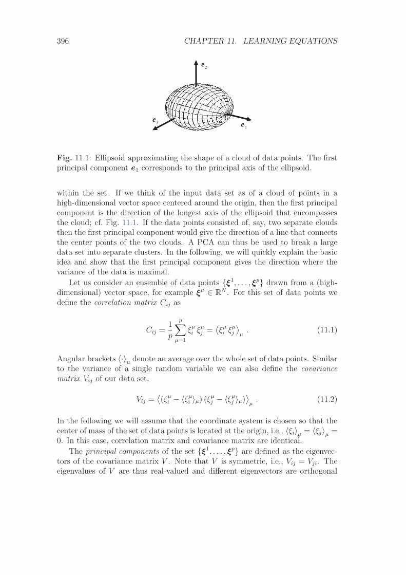
396 CHAPTER 11. LEARNING EQUATIONS
e1
e2
e3
Fig. 11.1: Ellipsoid approximating the shape of a cloud of data points. The firstprincipal component e1 corresponds to the principal axis of the ellipsoid.
within the set. If we think of the input data set as of a cloud of points in ahigh-dimensional vector space centered around the origin, then the first principalcomponent is the direction of the longest axis of the ellipsoid that encompassesthe cloud; cf. Fig. 11.1. If the data points consisted of, say, two separate cloudsthen the first principal component would give the direction of a line that connectsthe center points of the two clouds. A PCA can thus be used to break a largedata set into separate clusters. In the following, we will quickly explain the basicidea and show that the first principal component gives the direction where thevariance of the data is maximal.
Let us consider an ensemble of data points {ξ1, . . . , ξp} drawn from a (high-dimensional) vector space, for example ξμ ∈ R
N . For this set of data points wedefine the correlation matrix Cij as
Cij =1
p
p∑μ=1
ξμi ξμ
j =⟨ξμi ξμ
j
⟩μ
. (11.1)
Angular brackets 〈·〉μ denote an average over the whole set of data points. Similarto the variance of a single random variable we can also define the covariancematrix Vij of our data set,
Vij =⟨(ξμ
i − 〈ξμi 〉μ) (ξμ
j − 〈ξμj 〉μ)
⟩μ
. (11.2)
In the following we will assume that the coordinate system is chosen so that thecenter of mass of the set of data points is located at the origin, i.e., 〈ξi〉μ = 〈ξj〉μ =0. In this case, correlation matrix and covariance matrix are identical.
The principal components of the set {ξ1, . . . , ξp} are defined as the eigenvec-tors of the covariance matrix V . Note that V is symmetric, i.e., Vij = Vji. Theeigenvalues of V are thus real-valued and different eigenvectors are orthogonal
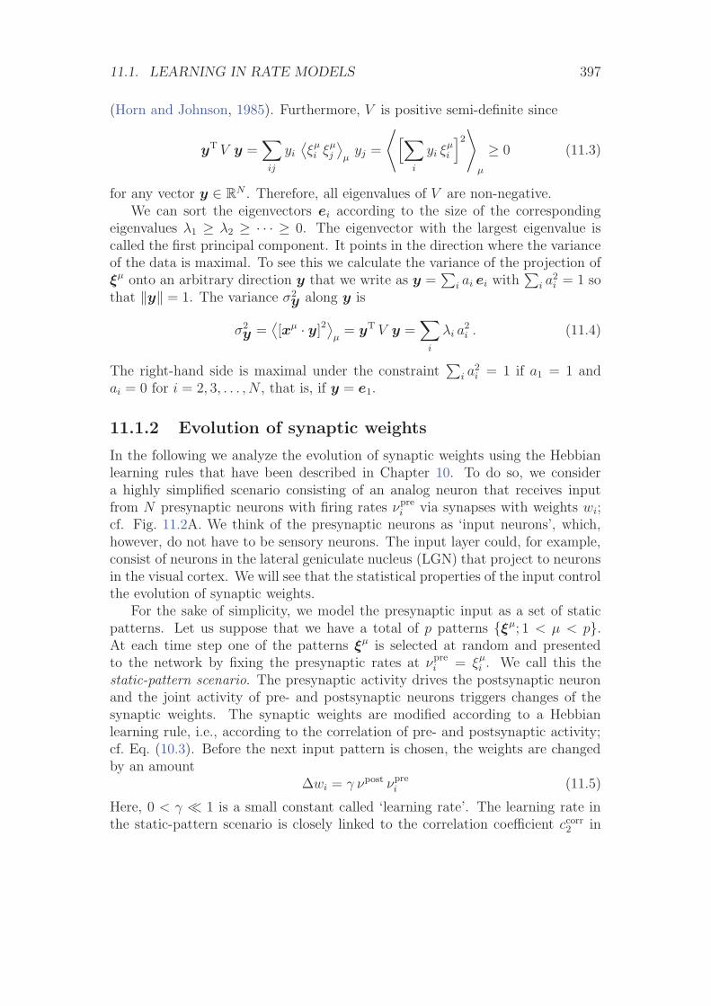
11.1. LEARNING IN RATE MODELS 397
(Horn and Johnson, 1985). Furthermore, V is positive semi-definite since
yT V y =∑ij
yi
⟨ξμi ξμ
j
⟩μ
yj =
⟨[∑i
yi ξμi
]2⟩
μ
≥ 0 (11.3)
for any vector y ∈ RN . Therefore, all eigenvalues of V are non-negative.
We can sort the eigenvectors ei according to the size of the correspondingeigenvalues λ1 ≥ λ2 ≥ · · · ≥ 0. The eigenvector with the largest eigenvalue iscalled the first principal component. It points in the direction where the varianceof the data is maximal. To see this we calculate the variance of the projection ofξμ onto an arbitrary direction y that we write as y =
∑i ai ei with
∑i a
2i = 1 so
that ‖y‖ = 1. The variance σ2y along y is
σ2y =
⟨[xμ · y]2
⟩μ
= yT V y =∑
i
λi a2i . (11.4)
The right-hand side is maximal under the constraint∑
i a2i = 1 if a1 = 1 and
ai = 0 for i = 2, 3, . . . , N , that is, if y = e1.
11.1.2 Evolution of synaptic weights
In the following we analyze the evolution of synaptic weights using the Hebbianlearning rules that have been described in Chapter 10. To do so, we considera highly simplified scenario consisting of an analog neuron that receives inputfrom N presynaptic neurons with firing rates νpre
i via synapses with weights wi;cf. Fig. 11.2A. We think of the presynaptic neurons as ‘input neurons’, which,however, do not have to be sensory neurons. The input layer could, for example,consist of neurons in the lateral geniculate nucleus (LGN) that project to neuronsin the visual cortex. We will see that the statistical properties of the input controlthe evolution of synaptic weights.
For the sake of simplicity, we model the presynaptic input as a set of staticpatterns. Let us suppose that we have a total of p patterns {ξμ; 1 < μ < p}.At each time step one of the patterns ξμ is selected at random and presentedto the network by fixing the presynaptic rates at νpre
i = ξμi . We call this the
static-pattern scenario. The presynaptic activity drives the postsynaptic neuronand the joint activity of pre- and postsynaptic neurons triggers changes of thesynaptic weights. The synaptic weights are modified according to a Hebbianlearning rule, i.e., according to the correlation of pre- and postsynaptic activity;cf. Eq. (10.3). Before the next input pattern is chosen, the weights are changedby an amount
Δwi = γ νpost νprei (11.5)
Here, 0 < γ 1 is a small constant called ‘learning rate’. The learning rate inthe static-pattern scenario is closely linked to the correlation coefficient ccorr
2 in
398 CHAPTER 11. LEARNING EQUATIONS
A Bν1
pre
νN
pre
.
.
.
.
.
μξ
wN
w1
νpost
ν post
h
h
0
g(h)
Fig. 11.2: Elementary model. A. Patterns ξμ are applied as a set of presynapticfiring rates νj, i.e., ξμ
j = νprej for 1 ≤ j ≤ N . B. The gain function of the postsy-
naptic neuron is taken as linear, i.e., νpost = h. It can be seen as a linearizationof the sigmoidal gain function g(h).
the continuous-time Hebb rule introduced in Eq. (10.3). In order to highlight therelation, let us assume that each pattern ξμ is applied during an interval Δt. ForΔt sufficiently small, we have γ = ccorr
2 Δt.In a general rate model, the firing rate νpost of the postsynaptic neuron is
given by a nonlinear function of the total input
νpost = g
(∑i
wi νprei
); (11.6)
cf. Fig. 11.2B. For the sake of simplicity, we restrict our discussion in the followingto a linear rate model with
νpost =∑
i
wi νprei . (11.7)
Obviously, this is a highly simplified neuron model, but it will serve our purposeof gaining some insights in the evolution of synaptic weights.
If we combine the learning rule (11.5) with the linear rate model of Eq. (11.7)we find after the presentation of pattern ξμ
Δwi = γ∑
j
wj νprej νpre
i = γ∑
j
wj ξμj ξμ
i . (11.8)
The evolution of the weight vector w = (w1, . . . , wN) is thus determined by theiteration
wi(n + 1) = wi(n) + γ∑
j
wj ξμn
j ξμn
i , (11.9)
where μn denotes the pattern that is presented during the nth time step.We are interested in the long-term behavior of the synaptic weights. To this
end we assume that the weight vector evolves along a more or less deterministic
11.1. LEARNING IN RATE MODELS 399
trajectory with only small stochastic deviations that result from the randomnessat which new input patterns are chosen. This is, for example, the case if thelearning rate is small so that a large number of patterns has to be presented inorder to induce a substantial weight change. In such a situation it is sensible toconsider the expectation value of the weight vector, i.e., the weight vector 〈w(n)〉averaged over the sequence (ξμ1 , ξμ2 , . . . , ξμn) of all patterns that so far have beenpresented to the network. From Eq. (11.9) we find
〈wi(n + 1)〉 = 〈wi(n)〉+ γ∑
j
⟨wj(n) ξ
μn+1
j ξμn+1
i
⟩= 〈wi(n)〉+ γ
∑j
〈wj(n)〉 ⟨ξμn+1
j ξμn+1
i
⟩= 〈wi(n)〉+ γ
∑j
Cij 〈wj(n)〉 . (11.10)
The angular brackets denote an ensemble average over the whole sequence of inputpatterns (ξμ1 , ξμ2 , . . . ). The second equality is due to the fact that input patternsare chosen independently in each time step, so that the average over wj(n) and(ξ
μn+1
j ξμn+1
i ) can be factorized. In the final expression we have introduced thecorrelation matrix Cij,
Cij =1
p
p∑μ=1
ξμi ξμ
j =⟨ξμi ξμ
j
⟩μ
. (11.11)
Expression (11.10) can be written in a more compact form using matrix notation,
〈w(n + 1)〉 = (1I + γ C) 〈w(n)〉 = (1I + γ C)n+1 〈w(0)〉 , (11.12)
where w(n) = (w1(n), . . . , wN(n)) is the weight vector and 1I is the identitymatrix.
If we express the weight vector in terms of the eigenvectors ek of C,
〈w(n)〉 =∑
k
ak(n) ek , (11.13)
we obtain an explicit expression for 〈w(n)〉 for any given initial condition ak(0),viz.,
〈w(n)〉 =∑
k
(1 + λk)n ak(0) ek . (11.14)
Since the correlation matrix is positive semi-definite all eigenvalues λk are real andpositive. Therefore, the weight vector is growing exponentially, but the growthwill soon be dominated by the eigenvector with the largest eigenvalue, i.e., thefirst principal component,
〈w(n)〉 n→∞−−−→ (1 + λ1)n a1(0) e1 ; (11.15)
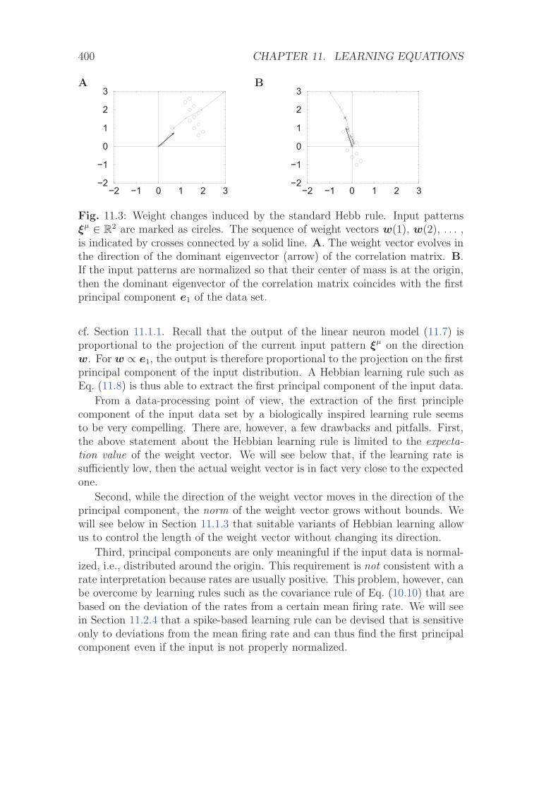
400 CHAPTER 11. LEARNING EQUATIONS
A B
−2 −1 0 1 2 3−2
−1
0
1
2
3
−2 −1 0 1 2 3−2
−1
0
1
2
3
Fig. 11.3: Weight changes induced by the standard Hebb rule. Input patternsξμ ∈ R
2 are marked as circles. The sequence of weight vectors w(1), w(2), . . . ,is indicated by crosses connected by a solid line. A. The weight vector evolves inthe direction of the dominant eigenvector (arrow) of the correlation matrix. B.If the input patterns are normalized so that their center of mass is at the origin,then the dominant eigenvector of the correlation matrix coincides with the firstprincipal component e1 of the data set.
cf. Section 11.1.1. Recall that the output of the linear neuron model (11.7) isproportional to the projection of the current input pattern ξμ on the directionw. For w ∝ e1, the output is therefore proportional to the projection on the firstprincipal component of the input distribution. A Hebbian learning rule such asEq. (11.8) is thus able to extract the first principal component of the input data.
From a data-processing point of view, the extraction of the first principlecomponent of the input data set by a biologically inspired learning rule seemsto be very compelling. There are, however, a few drawbacks and pitfalls. First,the above statement about the Hebbian learning rule is limited to the expecta-tion value of the weight vector. We will see below that, if the learning rate issufficiently low, then the actual weight vector is in fact very close to the expectedone.
Second, while the direction of the weight vector moves in the direction of theprincipal component, the norm of the weight vector grows without bounds. Wewill see below in Section 11.1.3 that suitable variants of Hebbian learning allowus to control the length of the weight vector without changing its direction.
Third, principal components are only meaningful if the input data is normal-ized, i.e., distributed around the origin. This requirement is not consistent with arate interpretation because rates are usually positive. This problem, however, canbe overcome by learning rules such as the covariance rule of Eq. (10.10) that arebased on the deviation of the rates from a certain mean firing rate. We will seein Section 11.2.4 that a spike-based learning rule can be devised that is sensitiveonly to deviations from the mean firing rate and can thus find the first principalcomponent even if the input is not properly normalized.
11.1. LEARNING IN RATE MODELS 401
Self-averaging (*)
So far, we have derived the behavior of the expected weight vector, 〈w〉. Herewe show that explicit averaging is not necessary provided that learning is slowenough. In this case, the weight vector is the sum of a large number of smallchanges. The weight dynamics is thus ‘self-averaging’ and the weight vector wcan be well approximated by its expectation value 〈w〉.
We start from the formulation of Hebbian plasticity in continuous time,
d
dtwi = ccorr
2 νpost νprei ; (11.16)
cf. Eq. (10.3). Each pattern ξμ is presented for a short period of duration Δt.We assume that the weights change during the presentation by a small amountonly, i.e.,
∫ t+Δt
t[dwj(t
′)/dt′] dt′ wj(t). This condition can be met either by ashort presentation time Δt or by a small learning coefficient ccorr
2 . Under thiscondition, we can take the postsynaptic firing rate νpost(t) =
∑j wj(t) νpre
i asconstant for the duration of one presentation. The total weight change inducedby the presentation of pattern ξμ to first order in Δt is thus
Δwi(t) = wi(t + Δt)− wi(t) = γ∑
j
wj(t) ξμj ξμ
i +O(Δt2) . (11.17)
with γ = ccorr2 Δt; cf. Eq. (11.8).
In the next time step a new pattern ξν is presented so that the weight ischanged to
wi(t + 2Δt) = wi(t + Δt) + ccorr2 Δt
∑j
wj(t + Δt) ξνj ξν
i +O(Δt2) . (11.18)
Since we keep only terms to first order in Δt, we may set wj(t + Δt) = wj(t) inthe sum on the right-hand side of Eq. (11.18). Let us suppose that in the interval[t, t + p Δt] each of the p patterns has been applied exactly once. Then, to firstorder in Δt,
wi(t + p Δt)− wi(t) = ccorr2 Δt
∑j
wj(t)
p∑μ=1
ξμi ξμ
j +O(Δt2) . (11.19)
For ccorr2 Δt 1, all higher-order terms can be neglected. Division by p Δt yields
wi(t + p Δt)− wi(t)
p Δt= ccorr
2
∑j
wj(t) Cij . (11.20)
The left-hand side can be approximated by a differential operator dw/dt,
d
dtwi(t) = ccorr
2
∑j
wj(t) Cij . (11.21)
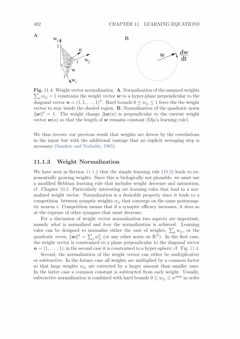
402 CHAPTER 11. LEARNING EQUATIONS
A
w1
������������������������������������������������������������������������������������������� � � � �� � � � �
���������������������������������������������������������������������������������������������������� � � � �
1
1
w
w2
31
n
w
B
dwdtw
Fig. 11.4: Weight vector normalization. A. Normalization of the summed weights∑j wij = 1 constrains the weight vector w to a hyper-plane perpendicular to the
diagonal vector n = (1, 1, . . . , 1)T . Hard bounds 0 ≤ wij ≤ 1 force the the weightvector to stay inside the shaded region. B. Normalization of the quadratic norm‖w‖2 = 1. The weight change Δw(n) is perpendicular to the current weightvector w(n) so that the length of w remains constant (Oja’s learning rule).
We thus recover our previous result that weights are driven by the correlationsin the input but with the additional vantage that no explicit averaging step isnecessary (Sanders and Verhulst, 1985).
11.1.3 Weight Normalization
We have seen in Section 11.1.2 that the simple learning rule (10.3) leads to ex-ponentially growing weights. Since this is biologically not plausible, we must usea modified Hebbian learning rule that includes weight decrease and saturation;cf. Chapter 10.2. Particularly interesting are learning rules that lead to a nor-malized weight vector. Normalization is a desirable property since it leads to acompetition between synaptic weights wij that converge on the same postsynap-tic neuron i. Competition means that if a synaptic efficacy increases, it does soat the expense of other synapses that must decrease.
For a discussion of weight vector normalization two aspects are important,namely what is normalized and how the normalization is achieved. Learningrules can be designed to normalize either the sum of weights,
∑j wij, or the
quadratic norm, ‖w‖2 =∑
j w2ij (or any other norm on R
N). In the first case,the weight vector is constrained to a plane perpendicular to the diagonal vectorn = (1, . . . , 1); in the second case it is constrained to a hyper-sphere; cf. Fig. 11.4.
Second, the normalization of the weight vector can either be multiplicativeor subtractive. In the former case all weights are multiplied by a common factorso that large weights wij are corrected by a larger amount than smaller ones.In the latter case a common constant is subtracted from each weight. Usually,subtractive normalization is combined with hard bounds 0 ≤ wij ≤ wmax in order
11.1. LEARNING IN RATE MODELS 403
to avoid runaway of individual weights. Finally, learning rules may or may notfall into the class of local learning rules that we have considered in Chapter 10.2.
A systematic classification of various learning rules according to the abovethree criteria has been proposed by Miller and MacKay (1994). Here we restrictourselves to two instances of learning with normalization properties which weillustrate in the examples below. We start with the subtractive normalizationof the summed weights
∑j wij and turn then to a discussion of Oja’s rule as an
instance of a multiplicative normalization of∑
j w2ij.
Example: Subtractive Normalization of∑
i wi
In a subtractive normalization scheme the sum over all weights,∑
i wi, can bekept constant by subtracting the average total weight change, N−1
∑i Δwi, from
each synapse after the weights have been updated according to a Hebbian learningrule with Δwi = γ
∑j wj ξμ
j ξμi . Altogether, the learning rule is of the form
Δwi = Δwi −N−1∑
j
Δwj
= γ(∑
j
wj ξμj ξμ
i −N−1∑
k
∑j
wj ξμj ξμ
k
), (11.22)
where Δwi denotes the weight change that is due to the pure Hebbian learningrule without the normalization. It can easily be verified that
∑i Δwi = 0 so that∑
i wi = const. The temporal evolution of the weight vector w is thus restrictedto a hyperplane perpendicular to (1, . . . , 1) ∈ R
N . Note that this learning rule isnon-local because the change of weight depends on the activity of all presynapticneurons.
In a similar way as in the previous section, we calculate the expectation of theweight vector 〈w(n)〉, averaged over the sequence of input patterns (ξμ1 , ξμ2 , . . . ),
〈wi(n + 1)〉 = 〈wi(n)〉+γ(∑
j
Cij 〈wj(n)〉−N−1∑
k
∑j
Ckj 〈wj(n)〉)
, (11.23)
or explicitly, using matrix notation
〈w(n)〉 = [1 + γ (C − C)]n 〈w(0)〉 , (11.24)
with Cij = N−1∑
k Ckj. The evolution of the weight vector is thus determined byeigenvectors of the matrix (C − C) that are in general different from those of thecorrelation matrix C. Hebbian learning with subtractive normalization is drivenby the correlations of the input in the subspace orthogonal to the diagonal vector(1, . . . , 1). Though the sum of the weights stays constant individual weights keepgrowing. It is thus necessary to adopt an additional criterion to stop the learning
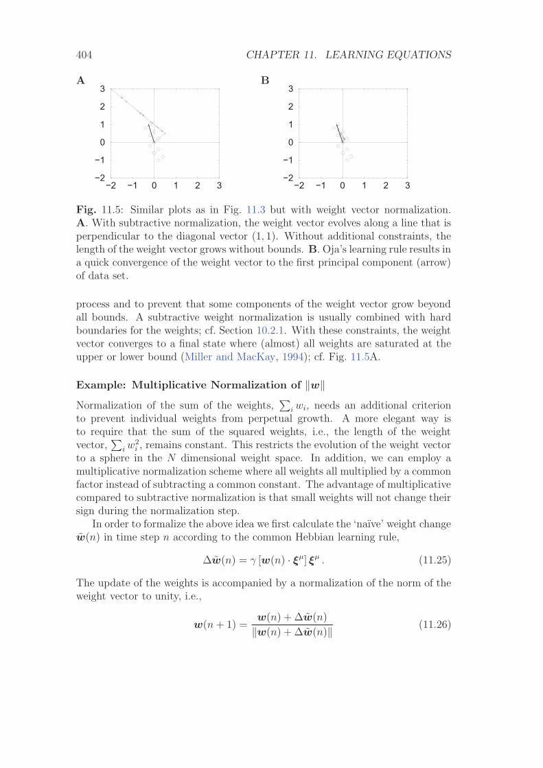
404 CHAPTER 11. LEARNING EQUATIONS
A B
−2 −1 0 1 2 3−2
−1
0
1
2
3
−2 −1 0 1 2 3−2
−1
0
1
2
3
Fig. 11.5: Similar plots as in Fig. 11.3 but with weight vector normalization.A. With subtractive normalization, the weight vector evolves along a line that isperpendicular to the diagonal vector (1, 1). Without additional constraints, thelength of the weight vector grows without bounds. B. Oja’s learning rule results ina quick convergence of the weight vector to the first principal component (arrow)of data set.
process and to prevent that some components of the weight vector grow beyondall bounds. A subtractive weight normalization is usually combined with hardboundaries for the weights; cf. Section 10.2.1. With these constraints, the weightvector converges to a final state where (almost) all weights are saturated at theupper or lower bound (Miller and MacKay, 1994); cf. Fig. 11.5A.
Example: Multiplicative Normalization of ‖w‖Normalization of the sum of the weights,
∑i wi, needs an additional criterion
to prevent individual weights from perpetual growth. A more elegant way isto require that the sum of the squared weights, i.e., the length of the weightvector,
∑i w
2i , remains constant. This restricts the evolution of the weight vector
to a sphere in the N dimensional weight space. In addition, we can employ amultiplicative normalization scheme where all weights all multiplied by a commonfactor instead of subtracting a common constant. The advantage of multiplicativecompared to subtractive normalization is that small weights will not change theirsign during the normalization step.
In order to formalize the above idea we first calculate the ‘naıve’ weight changew(n) in time step n according to the common Hebbian learning rule,
Δw(n) = γ [w(n) · ξμ] ξμ . (11.25)
The update of the weights is accompanied by a normalization of the norm of theweight vector to unity, i.e.,
w(n + 1) =w(n) + Δw(n)
‖w(n) + Δw(n)‖ (11.26)
11.1. LEARNING IN RATE MODELS 405
If we assume that the weights are changed only by a very small amount duringeach step (γ 1), we can calculate the new weights w(n + 1) to first order in γ,
w(n + 1) = w(n) + Δw(n)−w(n) [w(n) ·Δw(n)] +O(γ2) . (11.27)
The ‘effective’ weight change Δw(n) including normalization to leading order inγ is thus
Δw(n) = Δw(n)−w(n) [w(n) ·Δw(n)] , (11.28)
which corresponds to the vector component of Δw that is orthogonal to thecurrent weight vector w. This is exactly what we would have expected becausethe length of the weight vector must stay constant; cf. Fig. 11.4B.
We may wonder whether Eq. (11.28) is a local learning rule. In order toanswer this question, we recall that the ‘naıve’ weight change Δwj = γ νpost νpre
j
uses only pre- and postsynaptic information. Hence, we can rewrite Eq. (11.28)in terms of the firing rates,
Δwj = γ νpost νj − γ wj(n)(νpost
)2. (11.29)
In the second term on the right-hand side we have made use of the linear neuronmodel, i.e., νpost =
∑k wk νpre
k . Since the weight change depends only on pre-and postsynaptic rates, Eq. (11.29), which is known as Oja’s learning rule (Oja,1982), is indeed local; cf. Eq. (10.11).
In order to see that Oja’s learning rule selects the first principal component weshow that the eigenvectors {e1, . . . , eN} of C are fixed points of the dynamics butthat only the eigenvector e1 with the largest eigenvalue is stable. For any fixedweight vector w we can calculate the expectation of the weight change in the nexttime step by averaging over the whole ensemble of input patterns {ξ1, ξ2, . . . }.With 〈Δw(n)〉 = γ C w we find from Eq. (11.28)
〈Δw〉 = γ C w − γ w [w · C w] , (11.30)
We claim that any eigenvector ei of the correlation matrix C is a fixed point ofEq. (11.30). Indeed, if we substitute w = ei in the above equation we find that〈Δw〉 = 0. In order to investigate the stability of this fixed point we considera small perturbation w = ei + c ej in the direction of ej . Here, |c| 1 is theamplitude of the perturbation. If we substitute w = ei + c ej into Eq. (11.30) wefind
〈Δw〉 = c γ (λj − λi) ej +O(c2) . (11.31)
The weight vector will thus evolve in the direction of the perturbation ej ifλj > λi so that initial perturbation will increase. In this case, ei is unstable.On the other hand, if λj < λi the averaged weight change tends to decrease theperturbation and ei is stable. Consequently, the eigenvector of C with the largesteigenvalue, viz., the first principle component, is the sole stable fixed point of thedynamics generated by the learning rule of Eq. (11.26). Figure 11.5B shows asimple example.
406 CHAPTER 11. LEARNING EQUATIONS
11.1.4 Receptive Field Development
Most neurons of the visual system respond only to stimulation from a narrowregion within the visual field. This region is called the receptive field of thatneuron. Depending on the precise position of a narrow bright spot within thereceptive field the corresponding neuron can either show an increase or a decreaseof the firing rate relative to its spontaneous activity at rest. The receptive fieldis subdivided accordingly into ‘ON’ and ‘OFF’ regions in order to further char-acterize neuronal response properties. Bright spots in an ON region increase thefiring rate whereas bright spots in an OFF region inhibit the neuron.
Different neurons have different receptive fields, but as a general rule, neigh-boring neurons have receptive fields that ‘look’ at about the same region of thevisual field. This is what is usually called the retinotopic organization of theneuronal projections – neighboring points in the visual field are mapped to neigh-boring neurons of the visual system.
The visual system forms a complicated hierarchy of interconnected corticalareas where neurons show increasingly complex response properties from onelayer to the next. Neurons from the lateral geniculate nucleus (LGN), which isthe first neuronal relay of visual information after the retina, are characterized byso-called center-surround receptive fields. These are receptive fields that consistof two concentric parts, an ON region and an OFF region. LGN neurons come intwo flavors, as ON-center and OFF-center cells. ON-center cells have a ON-regionin the center of their receptive field that is surrounded by a circular OFF-region.In OFF-center cells the arrangement is the other way round; a central OFF-regionis surrounded by an ON-region; cf. Fig. 11.6.
Neurons from the LGN project to the primary visual cortex (V1), which isthe first cortical area involved in the processing of visual information. In thisarea neurons can be divided into ‘simple cells’ and ’complex cells’. In contrastto LGN neurons, simple cells have asymmetric receptive fields which results ina selectivity with respect to the orientation of a visual stimulus. The optimalstimulus for a neuron with a receptive field such as that shown in Fig. 11.6D, forexample, is a light bar tilted by about 45 degrees. Any other orientation wouldalso stimulate the OFF region of the receptive field leading to a reduction of theneuronal response. Complex cells have even more intriguing properties and showresponses that are, for example, selective for movements with a certain velocityand direction (Hubel, 1995).
It is still a matter of debate how the response properties of simple cells arise.The original proposal by Hubel and Wiesel (1962) was that orientation selec-tivity is a consequence of the specific wiring between LGN and V1. Severalcenter-surround cells with slightly shifted receptive fields should converge on asingle V1 neuron so as to produce the asymmetric receptive field of simple cells.Alternatively (or additionally), the intra-cortical dynamics can generate orienta-
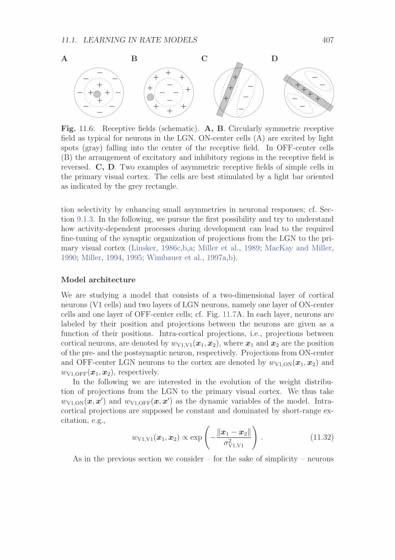
11.1. LEARNING IN RATE MODELS 407
A
−
−
−−
−
−
−+
++ −
+
B
+
+
+−
+
+
−−−
+
+
+
C
+++
−−−
D
++−
−
−−++
Fig. 11.6: Receptive fields (schematic). A, B. Circularly symmetric receptivefield as typical for neurons in the LGN. ON-center cells (A) are excited by lightspots (gray) falling into the center of the receptive field. In OFF-center cells(B) the arrangement of excitatory and inhibitory regions in the receptive field isreversed. C, D. Two examples of asymmetric receptive fields of simple cells inthe primary visual cortex. The cells are best stimulated by a light bar orientedas indicated by the grey rectangle.
tion selectivity by enhancing small asymmetries in neuronal responses; cf. Sec-tion 9.1.3. In the following, we pursue the first possibility and try to understandhow activity-dependent processes during development can lead to the requiredfine-tuning of the synaptic organization of projections from the LGN to the pri-mary visual cortex (Linsker, 1986c,b,a; Miller et al., 1989; MacKay and Miller,1990; Miller, 1994, 1995; Wimbauer et al., 1997a,b).
Model architecture
We are studying a model that consists of a two-dimensional layer of corticalneurons (V1 cells) and two layers of LGN neurons, namely one layer of ON-centercells and one layer of OFF-center cells; cf. Fig. 11.7A. In each layer, neurons arelabeled by their position and projections between the neurons are given as afunction of their positions. Intra-cortical projections, i.e., projections betweencortical neurons, are denoted by wV1,V1(x1, x2), where x1 and x2 are the positionof the pre- and the postsynaptic neuron, respectively. Projections from ON-centerand OFF-center LGN neurons to the cortex are denoted by wV1,ON(x1, x2) andwV1,OFF(x1, x2), respectively.
In the following we are interested in the evolution of the weight distribu-tion of projections from the LGN to the primary visual cortex. We thus takewV1,ON(x, x′) and wV1,OFF(x, x′) as the dynamic variables of the model. Intra-cortical projections are supposed be constant and dominated by short-range ex-citation, e.g.,
wV1,V1(x1, x2) ∝ exp
(−‖x1 − x2‖
σ2V1,V1
). (11.32)
As in the previous section we consider – for the sake of simplicity – neurons
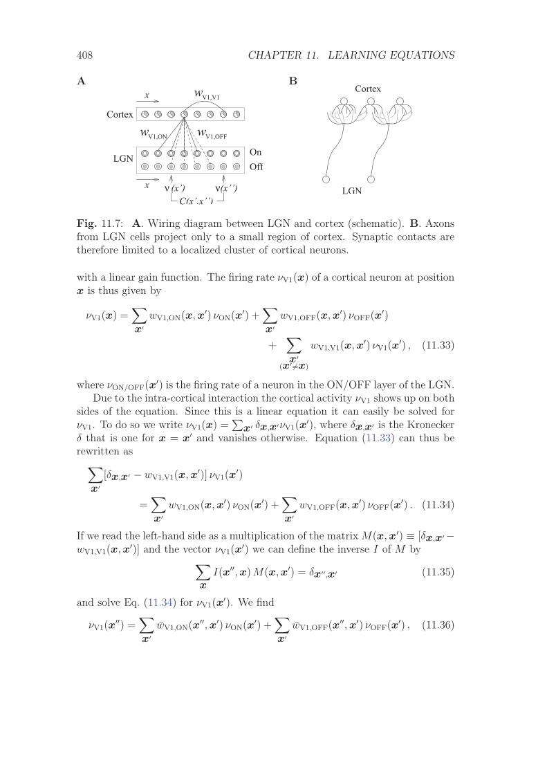
408 CHAPTER 11. LEARNING EQUATIONS
A B
V1,ONwOnOff
ν(x’’)(x’)
Cortex
LGN
V1,OFFw
V1,V1wx
x
C(x’,x’’)ν LGN
Cortex
Fig. 11.7: A. Wiring diagram between LGN and cortex (schematic). B. Axonsfrom LGN cells project only to a small region of cortex. Synaptic contacts aretherefore limited to a localized cluster of cortical neurons.
with a linear gain function. The firing rate νV1(x) of a cortical neuron at positionx is thus given by
νV1(x) =∑x′
wV1,ON(x, x′) νON(x′) +∑x′
wV1,OFF(x, x′) νOFF(x′)
+∑x′
(x′ �=x)
wV1,V1(x, x′) νV1(x′) , (11.33)
where νON/OFF(x′) is the firing rate of a neuron in the ON/OFF layer of the LGN.Due to the intra-cortical interaction the cortical activity νV1 shows up on both
sides of the equation. Since this is a linear equation it can easily be solved forνV1. To do so we write νV1(x) =
∑x′ δx,x′νV1(x
′), where δx,x′ is the Kroneckerδ that is one for x = x′ and vanishes otherwise. Equation (11.33) can thus berewritten as∑
x′[δx,x′ − wV1,V1(x, x′)] νV1(x
′)
=∑x′
wV1,ON(x, x′) νON(x′) +∑x′
wV1,OFF(x, x′) νOFF(x′) . (11.34)
If we read the left-hand side as a multiplication of the matrix M(x, x′) ≡ [δx,x′−wV1,V1(x, x′)] and the vector νV1(x
′) we can define the inverse I of M by∑x
I(x′′, x) M(x, x′) = δx′′,x′ (11.35)
and solve Eq. (11.34) for νV1(x′). We find
νV1(x′′) =
∑x′
wV1,ON(x′′, x′) νON(x′) +∑x′
wV1,OFF(x′′, x′) νOFF(x′) , (11.36)
11.1. LEARNING IN RATE MODELS 409
which relates the input νON/OFF to the output via the ‘effective’ weights
wV1,ON/OFF(x′′, x′) ≡∑x
I(x′′, x) wV1,ON/OFF(x, x′) . (11.37)
Plasticity
We expect that the formation of synapses between LGN and V1 is driven bycorrelations in the input. In the present case, these correlations are due to theretinotopic organization of projections from the retina to the LGN. NeighboringLGN neurons receiving stimulation from similar regions of the visual field are thuscorrelated to a higher degree than neurons that are more separated. If we assumethat the activity of individual photoreceptors on the retina is uncorrelated andthat each LGN neuron integrates the input from many of these receptors then thecorrelation of two LGN neurons can be calculated from the form of their receptivefields. For center-surround cells the correlation is a Mexican hat-shaped functionof their distance (Miller, 1994; Wimbauer et al., 1997a), e.g.,
CON,ON(x, x′) = CON,ON(‖x− x′‖)= exp
(−‖x − x′‖2
σ2
)− 1
c2exp
(−‖x− x′‖2
c2 σ2
), (11.38)
where c is a form factor that describes the depth of the modulation. CON,ON is thecorrelation between two ON-center type LGN neurons. For the sake of simplicitywe assume that OFF-center cells have the same correlation, COFF,OFF = CON,ON.Correlations between ON-center and OFF-center cells, however, have the oppositesign, CON,OFF = COFF,ON = −CON,ON.
In the present formulation of the model each LGN cell can contact everyneuron in the primary visual cortex. In reality, each LGN cell sends one axonto the cortex. Though this axon may split into several branches its synapticcontacts are restricted to small region of the cortex; cf. Fig. 11.7B. We take thislimitation into account by defining an arborization function A(x, x′) that givesthe a priori probability that a connection between a LGN cell at location x anda cortical cell at x′ is formed (Miller et al., 1989). The arborization is a rapidlydecaying function of the distance, e.g.,
A(x, x′) = exp
(−‖x − x′‖2
σ2V1,LGN
). (11.39)
To describe the dynamics of the weight distribution we adopt a modified formof Hebb’s learning rule that is completed by the arborization function,
d
dtwV1,ON/OFF(x, x′) = γ A(x, x′) νV1(x) νON/OFF(x′) . (11.40)
410 CHAPTER 11. LEARNING EQUATIONS
If we use Eq. (11.34) and assume that learning is slow enough so that we canrely on the correlation functions to describe the evolution of the weights, we find
d
dtwV1,ON(x1, x2) = γ A(x1, x2)
∑x′,x′′
I(x1, x′)
× [wV1,ON(x′, x′′) − wV1,OFF(x′, x′′)
]CON,ON(x′′, x2) (11.41)
and a similar equation for wV1,OFF.
Expression (11.41) is still a linear equation for the weights and nothing excit-ing can be expected. A prerequisite for pattern formation is competition betweenthe synaptic weights. Therefore, the above learning rule is extended by a termwV1,ON/OFF(x, x′) νV1(x)2 that leads to weight vector normalization and compe-tition; cf. Oja’s rule, Eq. (10.11).
Simulation results
Many of the standard techniques for nonlinear systems that we have alreadyencountered in the context of neuronal pattern formation in Chapter 9 can alsobe applied to the present model (MacKay and Miller, 1990; Wimbauer et al.,1998). Here, however, we will just summarize some results from a computersimulation consisting of an array of 8× 8 cortical neurons and two times 20× 20LGN neurons. Figure 11.8 shows a typical outcome of such a simulation. Eachof the small rectangles shows the receptive field of the corresponding corticalneuron. A bright color means that the neuron responds with an increased firingrate to a bright spot at that particular position within its receptive field; darkcolors indicate inhibition.
There are two interesting aspects. First, the evolution of the synaptic weightshas lead to asymmetric receptive fields, which give rise to orientation selectivity.Second, the structure of the receptive fields of neighboring cortical neurons aresimilar; neuronal response properties thus vary continuously across the cortex.The neurons are said to form a map for, e.g., orientation.
The first observation, the breaking of the symmetry of LGN receptive fields,is characteristic for all pattern formation phenomena. It results from the insta-bility of the homogeneous initial state and the competition between individualsynaptic weights. The second observation, the smooth variation of the receptivefields across the cortex, is a consequence of the excitatory intra-cortical couplings.During the development, neighboring cortical neurons tend to be either simulta-neously active or quiescent and due to the activity dependent learning rule similarreceptive fields are formed.
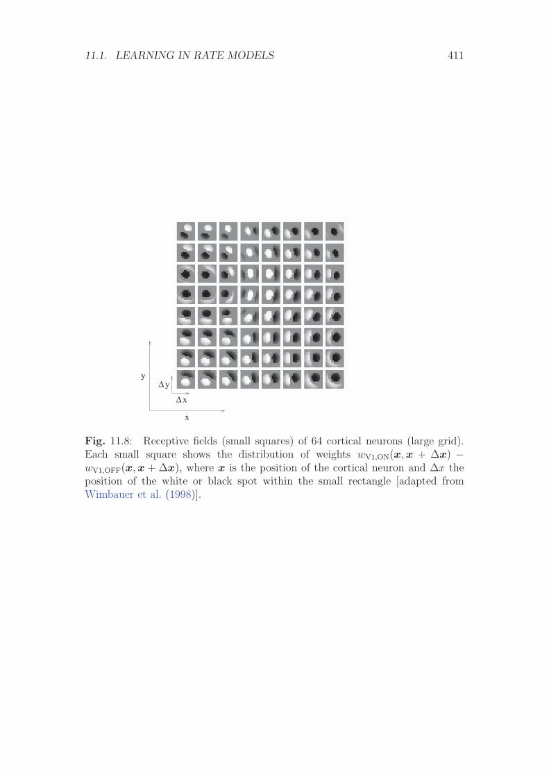
11.1. LEARNING IN RATE MODELS 411
Δ y
Δ
y
x
x
Fig. 11.8: Receptive fields (small squares) of 64 cortical neurons (large grid).Each small square shows the distribution of weights wV1,ON(x, x + Δx) −wV1,OFF(x, x + Δx), where x is the position of the cortical neuron and Δx theposition of the white or black spot within the small rectangle [adapted fromWimbauer et al. (1998)].
412 CHAPTER 11. LEARNING EQUATIONS
11.2 Learning in Spiking Models
In the previous section we have seen that the evolution of synaptic weights undera rate-based learning rule depends on correlations in the input. What happens,if the rate-based learning rule is replaced by a spike-time dependent one?
In Section 11.2.1 we will derive an equation that relates the expectation valueof the weight vector to statistical properties of pre- and postsynaptic spike trains.We will see that spike-time dependent plasticity is sensitive to spatial and tem-poral correlations in the input. In certain particularly simple cases spike-spikecorrelations can be calculated explicitly. This is demonstrated in Section 11.2.2in the context of a linear Poisson neuron. This neuron model is also used in Sec-tion 11.2.3 for a comparison of spike-based and rate-based learning rules as wellas in Section 11.2.4 where we revisit the static-pattern scenario of Section 11.1.2.Finally, in Section 11.2.5, we discuss the impact of stochastic spike arrival on thesynaptic weights and derive a Fokker-Planck equation that describes the temporalevolution of the weight distribution.
11.2.1 Learning Equation
We will generalize the analysis of Hebbian learning that has been developed inSection 11.1 to spike-based learning rules based on the phenomenological modelof Section 10.3.1. In this model the synaptic weight wij(t) is a piecewise contin-uous function of time with steps whenever a presynaptic spike arrives or when apostsynaptic action potential is triggered, i.e.,
d
dtwij(t) = a0 + apre
1 Sj(t) + apost1 Si(t)
+ Sj(t)
∫ ∞
0
W (s) Si(t− s) ds + Si(t)
∫ ∞
0
W (−s) Sj(t− s) ds , (11.42)
cf. Eqs. (10.14)–(10.15). As before we want to relate the synaptic weight changeto the statistical properties of the input. Given the increased level of complexity,a few remarks about the underlying statistical ensemble are in order.
In the previous section we have considered presynaptic firing rates νj as ran-dom variables drawn from an ensemble of input patterns ξμ
j . The output rate,however, was a deterministic function of the neuronal input. In the context ofspike-time dependent plasticity, we consider the set of presynaptic spike arrivaltimes (t1j , t
2j , . . . ) as a random variable. The underlying ‘randomness’ may have
several reasons. For example, different stimulation paradigms may be selectedone by one in very much the same way as we have selected a new input patternin the previous section. In contrast to the rate model, we do not want to restrictourselves to deterministic neuron models. Hence, the randomness can also beproduced by a stochastic neuron model that is used in order account for noise;
11.2. LEARNING IN SPIKING MODELS 413
cf. Chapter 5. In this case, the output spike train can be a random variable evenif the input spike trains are fixed. A simple example is the Poisson neuron modelthat generates output spikes via an inhomogeneous Poisson process with an inten-sity that is a function of the membrane potential. In any case, we consider the setof spike trains (S1, . . . , Si, Sj, . . . , SN), i.e., pre- and postsynaptic trains, to bedrawn from a stochastic ensemble. The specific properties of the chosen neuronmodel are thus implicitly described by the association of pre- and postsynaptictrains within the ensemble. Note that this formalism includes deterministic mod-els as a special case, if the ensemble contains only a single postsynaptic spiketrain for any given set of presynaptic spike trains. In the following, all averagesdenoted by 〈·〉E are to be taken relative to this ensemble.
For the time being we are interested only in the long-term behavior of thesynaptic weights and not in the fluctuations that are caused by individual spikes.As in Section 11.1.2 we therefore calculate the expectation value of the weightchange over a certain interval of time,
〈wij(t + T )− wij(t)〉E =
⟨∫ t+T
t
d
dtwij(t
′)dt′⟩
E
. (11.43)
With the abbreviation
〈f(t)〉T ≡ T−1
∫ t+T
t
f(t′) dt′ (11.44)
we obtain from Eq. (11.42)
〈wij(t + T )− wij(t)〉ET
= a0 + apre1
⟨⟨Sj(t)
⟩T
⟩E
+ apost1
⟨⟨Si(t)
⟩T
⟩E
+
∫ ∞
0
W (s)⟨⟨
Si(t− s) Sj(t)⟩
T
⟩E
ds
+
∫ 0
−∞W (s)
⟨⟨Si(t) Sj(t + s)
⟩T
⟩E
ds . (11.45)
If the time interval T is long as compared to typical interspike intervals then thetime average is taken over many pre- or postsynaptic spikes. We can thus assumethat the average
⟨⟨Si(t) Sj(t + s)
⟩T
⟩E
does not change if we replace t by t− s aslong as s T . Furthermore, if W (s) decays to zero sufficiently fast as |s| → ∞then the integration over s in the last term of Eq. (11.45) can be restricted to afinite interval determined by the width of the learning window W . In this case itis possible to replace
⟨⟨Si(t) Sj(t+ s)
⟩T
⟩E
by⟨⟨
Si(t− s) Sj(t)⟩
T
⟩E
and to collectthe last two terms of Eq. (11.45) into a single integral, provided that the width
414 CHAPTER 11. LEARNING EQUATIONS
of learning window is small as compared to T . With this approximation we find
〈wij(t + T )− wij(t)〉ET
= a0 + apre1
⟨⟨Sj(t)
⟩T
⟩E
+ apost1
⟨⟨Si(t)
⟩T
⟩E
+
∫ ∞
−∞W (s)
⟨⟨Si(t− s) Sj(t)
⟩T
⟩E
ds . (11.46)
The instantaneous firing rate νi(t) of neuron i is the ensemble average of itsspike train,
νi(t) ≡⟨Si(t)
⟩E
. (11.47)
Similarly, we define the joint firing rate νij of neuron i and j as
νij(t, t′) ≡ ⟨
Si(t) Sj(t′)⟩
E, (11.48)
which is the joint probability density to find both a spike at time t and at timet′ in neuron i and j, respectively. Note that νij(t, t
′) is a probability density bothin t and t′ and thus has units of one over time squared.
Since averaging is a linear operations we can exchange ensemble average andtime average. We obtain the following expression for the expected weight changein the interval from t to t + T as a function of the statistical properties of thespike trains,
〈wij(t + T )− wij(t)〉ET
= a0 + apre1
⟨νj(t)
⟩T
+ apost1
⟨νi(t)
⟩T
+
∫ ∞
−∞W (s)
⟨νij(t− s, t)
⟩T
ds . (11.49)
The time average 〈νij(t − s, t)〉T is the correlation function of pre- and post-synaptic spike train on the interval [t, t + T ]. This function clearly depends onthe actual value of the weight vector. In deriving Eq. (11.49) we already had toassume that the correlations are a slowly varying function of time. For the sake ofconsistency we thus have the requirement that the weight vector itself is a slowlyvarying function of time. If this is the case then we can exploit the self-averagingproperty of the weight vector and argue that fluctuations around the expectationvalue are negligible and that Eq. (11.49) is a good approximation for the actualvalue of the weight vector. We thus drop the ensemble average on the left-handside of Eq. (11.49) and find for the time-averaged change of the synaptic weightthe following learning equation,
d
dt
⟨wij(t)
⟩T
= a0 + apre1
⟨νj(t)
⟩T
+ apost1
⟨νi(t)
⟩T
+
∫ ∞
−∞W (s)
⟨νij(t− s, t)
⟩T
ds ; (11.50)
11.2. LEARNING IN SPIKING MODELS 415
cf. (Kempter et al., 1999; Kistler and van Hemmen, 2000a). As expected, thelong-term dynamics of the synaptic weights depends on the correlation of pre-and postsynaptic spike train on the time scale of the learning window. In thefollowing we will always use the smooth time-averaged weight vector 〈wij(t)〉T ,but for the sake of brevity we shall drop the angular brackets.
11.2.2 Spike-Spike Correlations
It is tempting to rewrite the correlation term 〈νij(t− s, t)〉T that appears on theright-hand side of Eq. (11.50) in terms of the instantaneous firing rates 〈νi(t −s) νj(t)〉T . This, however, is only allowed, if the spike trains of neuron i and j wereindependent, i.e., if 〈Si(t− s) Sj(t)〉E = 〈Si(t− s)〉E 〈Sj(t)〉E. Such an approachwould therefore neglect the specific spike-spike correlations that are induced bypresynaptic action potentials.
Correlations between pre- and postsynaptic spike trains do not only dependon the input statistics but also on the dynamics of the neuron model and theway new output spikes are generated. The influence of a single presynaptic spikeon the postsynaptic activity can be measured by a peri-stimulus time histogram(PSTH) triggered on the time of presynaptic spike arrival; cf. Section 7.4.1. Theform of the PSTH characterizes the spike-spike correlations between presynapticspike arrival and postsynaptic action potential. For high noise, the spike-spikecorrelations contain a term that is proportional to the time-course of the postsy-naptic potential ε, while for low noise this term is proportional to its derivativeε′; cf. Figs. 7.12.
In the following, we will calculate the spike-spike correlations in a particularlysimple case, the linear Poisson neuron model. As we will see, the spike-spikecorrelations contain in this case a term proportional to the postsynaptic potentialε. The linear Poisson neuron model can therefore be considered as a reasonableapproximation to spiking neuron models in the high-noise limit.
Example: Linear Poisson neuron model
As a generalization of the analog neuron with linear gain function discussed inSection 11.1.2 we consider here a linear Poisson neuron. The input to the neuronconsists of N Poisson spike trains with time-dependent intensities νj(t). Similarto the SRM0 neuron the membrane potential ui of neuron i is a superposition ofpostsynaptic potentials ε with
∫∞0
ε(s) ds = 1,
ui(t) =∑
j
wij
∫ ∞
0
ε(s) Sj(t− s) ds . (11.51)
In contrast to Section 4.2.3 we neglect refractoriness and external input.
416 CHAPTER 11. LEARNING EQUATIONS
Postsynaptic spikes are generated by an inhomogeneous Poisson process withan intensity νpost
i that is a (semi-)linear function of the membrane potential,
νposti (t|u) = [ui(t)]+ . (11.52)
Here, [·]+ denotes the positive part of the argument in order to avoid negativerates. In the following, however, we will always assume that ui(t) ≥ 0. Thenotation νpost
i (t|u) indicates that the output rate depends on the actual value ofthe membrane potential.
We thus have a doubly stochastic process (Cox, 1955; Bartlett, 1963) in thesense that in a first step, a set of input spike trains is drawn from an ensemblecharacterized by Poisson rates νpre
j . This realization of input spike trains thendetermines the membrane potential which produces in a second step a specificrealization of the output spike train according to νpost
i (t|u). It can be shown that,because of the finite duration of the postsynaptic potential ε, the output spiketrains generated by this composite process are no longer Poisson spike trains;their expectation value 〈Si(t)〉E ≡ νpost
i (t), however, is simply equivalent to theexpectation value of the output rate, νpost
i (t) = 〈νposti (t|u)〉E (Kistler and van
Hemmen, 2000a). Due to the linearity of the neuron model the output rate isgiven by a convolution of the input rates with the response kernel ε,
νposti (t) =
∑j
wij
∫ ∞
0
ε(s) νprej (t− s) ds . (11.53)
The joint firing rate νpost,preij (t, t′) = 〈Si(t) Sj(t
′)〉E of pre- and postsynapticneuron is the joint probability density to find an input spike at synapse j at timet′ and an output spike of neuron i at time t. According to Bayes’ Theorem thisprobability equals the probability of observing an input spike at time t′ timesthe conditional probability of observing an output spike at time t given the inputspike at time t′, i.e.,
νpost,preij (t, t′) = 〈Si(t)|input spike at t′〉E 〈Sj(t
′)〉E . (11.54)
In the framework of a linear Poisson neuron, the term 〈Si(t)|input spike at t′〉Eequals the sum of the expected output rate (11.53) and the specific contributionwij ε(t− t′) of a single (additional) input spike at time t′. Altogether we obtain
νpost,preij (t, t′) = νpost
i (t) νprej (t′) + wij ε(t− t′) νpre
j (t′) . (11.55)
The first term on the right-hand side is the ‘chance level’ to find two spikes att and t′, respectively, if the neurons were firing independently at rates νpost
i (t)and νpre
j (t′). The second term describes the correlation that is due to synapticcoupling. If the presynaptic neuron has fired a spike at t′ then the chance for thepostsynaptic neuron to fire an spike at time t > t′ is increased by wij ε(t−t′). Notethat this expression respects causality: The probability to find first a postsynapticspike and then a presynaptic spike is just chance level because ε(t − t′) = 0 fort < t′.
11.2. LEARNING IN SPIKING MODELS 417
Example: Learning equation for a linear Poisson neuron
If we use the result from Eq. (11.55) in the learning equation (11.50) we obtain
d
dtwij(t) = a0 + apre
1 〈νprej (t)〉T + apost
1 〈νposti (t)〉T
+
∫ ∞
−∞W (s) 〈νpost
i (t− s) νprej (t)〉T ds + wij(t) 〈νpre
j (t)〉T W− , (11.56)
with W− =∫∞
0W (−s) ε(s)ds.
In linear Poisson neurons, the correlation between pre- and postsynaptic ac-tivity that drives synaptic weight changes consists of two contributions. Theintegral over the learning window in Eq. (11.56) describes correlations in the in-stantaneous firing rate. The last term on the right-hand side of Eq. (11.56) finallyaccounts for spike-spike correlations of pre- and postsynaptic neuron.
If we express the instantaneous firing rates νi(t) in terms of their fluctuationsΔνi(t) around the mean 〈νi(t)〉T ,
νi(t) = Δνi(t) + 〈νi(t)〉T , (11.57)
then we can rewrite Eq. (11.56) together with Eq. (11.53) as
d
dtwij(t) = a0 + apre
1 〈νprej (t)〉T + apost
1 〈νposti (t)〉T
+ W 〈νprej (t)〉T 〈νpost
i (t)〉T +∑
k
wik Qkj(t) + wij(t) 〈νprej (t)〉T W− (11.58)
with
Qkj(t) =
∫ ∞
−∞W (s)
∫ ∞
0
ε(s′) 〈Δνprek (t− s− s′) Δνpre
j (t)〉T ds′ ds . (11.59)
Here we have implicitly assumed that the temporal averaging interval T is muchlonger than the length of the learning window, the duration of a postsynapticpotential, or a typical interspike interval, so that 〈νpost
i (t− s)〉T ≈ 〈νposti (t)〉T and
〈νprej (t− s′)〉T ≈ 〈νpre
j (t)〉T .The term containing Qkj(t) on the right-hand side of Eq. (11.58) shows how
spatio-temporal correlations 〈Δνpostk (t′) Δνpre
j (t)〉T in the input influence the evo-lution of synaptic weights. What matters are correlations on the time scale ofthe learning window and the postsynaptic potential.
11.2.3 Relation of spike-based to rate-based learning
In Section 11.1.2 we have investigated the weight dynamics in the context of ananalog neuron where the postsynaptic firing rate is an instantaneous function of
418 CHAPTER 11. LEARNING EQUATIONS
the input rates. We have seen that learning is driven by (spatial) correlationswithin the set of input patterns. The learning equation (11.56) goes one stepfurther in the sense that it explicitly includes time. Consequently, learning isdriven by spatio-temporal correlations in the input.
In order to compare the rate-based learning paradigm of Section 11.1.2 withthe spike-based formulation of Eq. (11.56) we thus have to disregard temporalcorrelations for the time being. We thus consider a linear Poisson neuron withstationary input rates, 〈νj(t)〉T = νj(t) = νj , and assume that the synapticweight is changing slowly as compared to the width of the learning window andthe postsynaptic potential. The weight dynamics is given by Eq. (11.56),
d
dtwij(t) = a0 + apre
1 νj + apost1 νi + W νi νj + W− wij(t) νj , (11.60)
with W =∫∞−∞W (s) ds and W− =
∫∞0
W (−s) ε(s)ds. If we identify
c0(wij) = a0 , cpre1 (wij) = apre
1 + wij(t) W− , cpost1 (wij) = apost
1 , (11.61)
andccorr2 (wij) = W , (11.62)
we recover the general expression for synaptic plasticity based on the rate descrip-tion given in Eq. (10.2). The total area under the learning window thus playsthe role of the correlation parameter ccorr
2 that is responsible for Hebbian or anti-Hebbian plasticity in a rate formulation. The spike-spike correlations simply giverise to an additional weight-dependent term wij(t) W− in the parameter cpre
1 (wij)that describes presynaptically triggered weight changes.
We may wonder what happens if we relax the requirement of strictly stationaryrates. In the linear Poisson model, the output rate depends via Eq. (11.53) onthe input rates and changes in the input rate translate into changes in the outputrate. If the rate of change is small, we can expand the output rate
νposti (t− s) ≈ νpost
i (t)− sd
dtνpost
i (t) +O(s2) (11.63)
on the right-hand side of Eq. (11.56),
d
dtwij(t) = a0 + apre
1 νprej (t) + apost
1 νposti (t) + W νpost
i (t) νprej (t)
+W−wij(t) νprej (t) − νpre
j (t)d
dtνpost
i (t)
∞∫−∞
s W (s) ds . (11.64)
Here, we have dropped the temporal averages because rates are assumed to changeslowly relative to T .
11.2. LEARNING IN SPIKING MODELS 419
As compared to Eq. (11.60) we encounter an additional term that is pro-portional to the first moment
∫s W (s) ds of the learning window. This term
has been termed differential -Hebbian (Roberts, 1999; Xie and Seung, 2000) andplays a certain role in the context of conditioning and reinforcement learning(Montague et al., 1995; Rao and Sejnowski, 2001).
Stabilization of Postsynaptic Rates
Another interesting property of a learning rule of the form (10.2) or (11.60) isthat it can lead to a normalization of the postsynaptic firing rate and hence toa normalization of the sum of the synaptic weights. This can be achieved evenwithout including higher order terms in the learning equation or postulating adependence of the parameters a0, a
pre/post1 , etc., on the actual value of the synaptic
efficacy.
Consider a linear Poisson neuron that receives input from N presynaptic neu-rons with spike activity described by independent Poisson processes with rateνpre. The postsynaptic neuron is thus firing at a rate νpost
i (t) = νpre∑N
j=1 wij(t).From Eq. (11.56) we obtain the corresponding dynamics for the synaptic weights,i.e.,
d
dtwij(t) = a0 + apre
1 νpre + apost1 νpre
N∑k=1
wik(t)
+ (νpre)2 W
N∑k=1
wik(t) + wij(t) νpre W− , (11.65)
with W =∫∞−∞W (s) ds and W− =
∫∞0
ε(s) W (−s) ds. In this particularly simplecase the weight dynamics is characterized by a fixed point for the sum of thesynaptic weights,
∑j wij, and, hence, for the postsynaptic firing rate, νpost
i = νFP,
νFP = − a0 + apre1 νpre
apost1 + νpre W + N−1 W−
. (11.66)
This fixed point is attractive if the denominator is negative. Since νposti is a
firing rate we have the additional requirement that νFP ≥ 0. Altogether we thushave two conditions for the parameters of the learning rule, i.e., apost
1 + νpre W +N−1 W− < 0 and a0 + apre
1 νpre ≥ 0. Note that we would obtain a – apart fromthe term (N−1 W−) – completely analogous result from the rate formulation inEq. (10.2) if we identify ccorr
2 = W ; cf. Eq. (11.62). Note further, that the linearityis not essential for the stabilization of the postsynaptic rate. Any model wherethe output rate is a monotonous function of the sum of the synaptic weights yieldsqualitatively the same result.
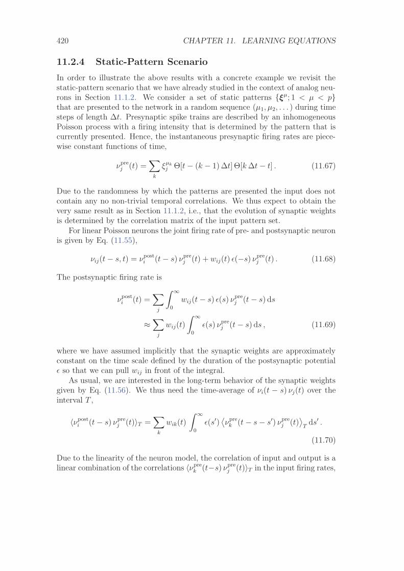
420 CHAPTER 11. LEARNING EQUATIONS
11.2.4 Static-Pattern Scenario
In order to illustrate the above results with a concrete example we revisit thestatic-pattern scenario that we have already studied in the context of analog neu-rons in Section 11.1.2. We consider a set of static patterns {ξμ; 1 < μ < p}that are presented to the network in a random sequence (μ1, μ2, . . . ) during timesteps of length Δt. Presynaptic spike trains are described by an inhomogeneousPoisson process with a firing intensity that is determined by the pattern that iscurrently presented. Hence, the instantaneous presynaptic firing rates are piece-wise constant functions of time,
νprej (t) =
∑k
ξμkj Θ[t− (k − 1) Δt] Θ[k Δt− t] . (11.67)
Due to the randomness by which the patterns are presented the input does notcontain any no non-trivial temporal correlations. We thus expect to obtain thevery same result as in Section 11.1.2, i.e., that the evolution of synaptic weightsis determined by the correlation matrix of the input pattern set.
For linear Poisson neurons the joint firing rate of pre- and postsynaptic neuronis given by Eq. (11.55),
νij(t− s, t) = νposti (t− s) νpre
j (t) + wij(t) ε(−s) νprej (t) . (11.68)
The postsynaptic firing rate is
νposti (t) =
∑j
∫ ∞
0
wij(t− s) ε(s) νprej (t− s) ds
≈∑
j
wij(t)
∫ ∞
0
ε(s) νprej (t− s) ds , (11.69)
where we have assumed implicitly that the synaptic weights are approximatelyconstant on the time scale defined by the duration of the postsynaptic potentialε so that we can pull wij in front of the integral.
As usual, we are interested in the long-term behavior of the synaptic weightsgiven by Eq. (11.56). We thus need the time-average of νi(t − s) νj(t) over theinterval T ,
〈νposti (t− s) νpre
j (t)〉T =∑
k
wik(t)
∫ ∞
0
ε(s′)⟨νpre
k (t− s− s′) νprej (t)
⟩T
ds′ .
(11.70)
Due to the linearity of the neuron model, the correlation of input and output is alinear combination of the correlations 〈νpre
k (t−s) νprej (t)〉T in the input firing rates,
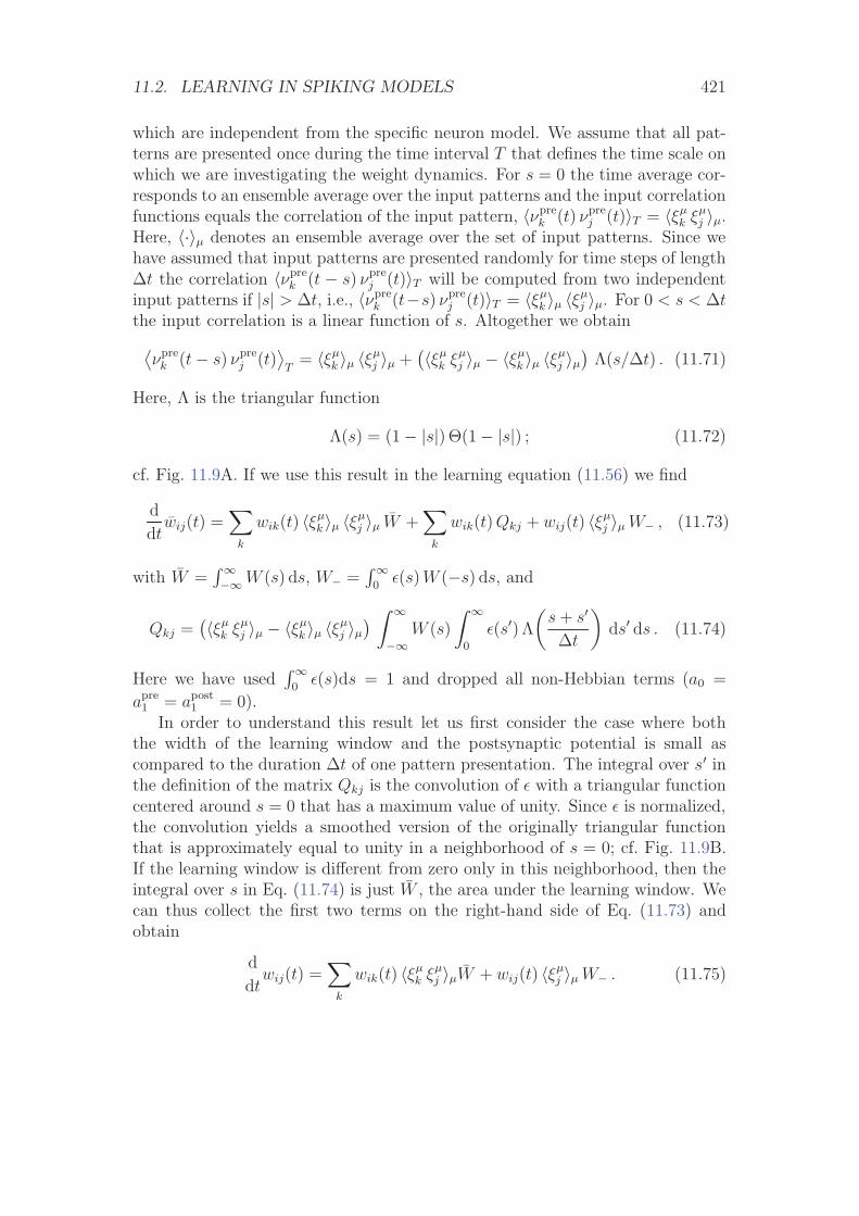
11.2. LEARNING IN SPIKING MODELS 421
which are independent from the specific neuron model. We assume that all pat-terns are presented once during the time interval T that defines the time scale onwhich we are investigating the weight dynamics. For s = 0 the time average cor-responds to an ensemble average over the input patterns and the input correlationfunctions equals the correlation of the input pattern, 〈νpre
k (t) νprej (t)〉T = 〈ξμ
k ξμj 〉μ.
Here, 〈·〉μ denotes an ensemble average over the set of input patterns. Since wehave assumed that input patterns are presented randomly for time steps of lengthΔt the correlation 〈νpre
k (t − s) νprej (t)〉T will be computed from two independent
input patterns if |s| > Δt, i.e., 〈νprek (t−s) νpre
j (t)〉T = 〈ξμk 〉μ 〈ξμ
j 〉μ. For 0 < s < Δtthe input correlation is a linear function of s. Altogether we obtain⟨
νprek (t− s) νpre
j (t)⟩
T= 〈ξμ
k 〉μ 〈ξμj 〉μ +
(〈ξμk ξμ
j 〉μ − 〈ξμk 〉μ 〈ξμ
j 〉μ)
Λ(s/Δt) . (11.71)
Here, Λ is the triangular function
Λ(s) = (1− |s|) Θ(1− |s|) ; (11.72)
cf. Fig. 11.9A. If we use this result in the learning equation (11.56) we find
d
dtwij(t) =
∑k
wik(t) 〈ξμk 〉μ 〈ξμ
j 〉μ W +∑
k
wik(t) Qkj + wij(t) 〈ξμj 〉μ W− , (11.73)
with W =∫∞−∞W (s) ds, W− =
∫∞0
ε(s) W (−s) ds, and
Qkj =(〈ξμ
k ξμj 〉μ − 〈ξμ
k 〉μ 〈ξμj 〉μ
) ∫ ∞
−∞W (s)
∫ ∞
0
ε(s′) Λ
(s + s′
Δt
)ds′ ds . (11.74)
Here we have used∫∞
0ε(s)ds = 1 and dropped all non-Hebbian terms (a0 =
apre1 = apost
1 = 0).In order to understand this result let us first consider the case where both
the width of the learning window and the postsynaptic potential is small ascompared to the duration Δt of one pattern presentation. The integral over s′ inthe definition of the matrix Qkj is the convolution of ε with a triangular functioncentered around s = 0 that has a maximum value of unity. Since ε is normalized,the convolution yields a smoothed version of the originally triangular functionthat is approximately equal to unity in a neighborhood of s = 0; cf. Fig. 11.9B.If the learning window is different from zero only in this neighborhood, then theintegral over s in Eq. (11.74) is just W , the area under the learning window. Wecan thus collect the first two terms on the right-hand side of Eq. (11.73) andobtain
d
dtwij(t) =
∑k
wik(t) 〈ξμk ξμ
j 〉μW + wij(t) 〈ξμj 〉μ W− . (11.75)
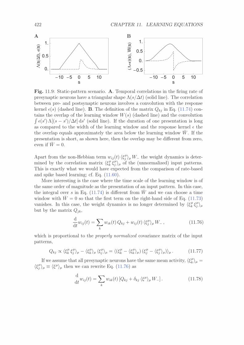
422 CHAPTER 11. LEARNING EQUATIONS
A
�10 �5 0 5 10s
0.
0.5
1.��s��
t�,Ε�
s�B
�10 �5 0 5 10s
�0.5
0.
0.5
1.
�����
s�,W�s�
Fig. 11.9: Static-pattern scenario. A. Temporal correlations in the firing rate ofpresynaptic neurons have a triangular shape Λ(s/Δt) (solid line). The correlationbetween pre- and postsynaptic neurons involves a convolution with the responsekernel ε(s) (dashed line). B. The definition of the matrix Qkj in Eq. (11.74) con-tains the overlap of the learning window W (s) (dashed line) and the convolution∫
ε(s′) Λ[(s − s′)/Δt] ds′ (solid line). If the duration of one presentation is longas compared to the width of the learning window and the response kernel ε thethe overlap equals approximately the area below the learning window W . If thepresentation is short, as shown here, then the overlap may be different from zero,even if W = 0.
Apart from the non-Hebbian term wij(t) 〈ξμj 〉μ W− the weight dynamics is deter-
mined by the correlation matrix 〈ξμk ξμ
j 〉μ of the (unnormalized) input patterns.This is exactly what we would have expected from the comparison of rate-basedand spike based learning; cf. Eq. (11.60).
More interesting is the case where the time scale of the learning window is ofthe same order of magnitude as the presentation of an input pattern. In this case,the integral over s in Eq. (11.74) is different from W and we can choose a timewindow with W = 0 so that the first term on the right-hand side of Eq. (11.73)vanishes. In this case, the weight dynamics is no longer determined by 〈ξμ
k ξμj 〉μ
but by the matrix Qjk,
d
dtwij(t) =
∑k
wik(t) Qkj + wij(t) 〈ξμj 〉μ W− , (11.76)
which is proportional to the properly normalized covariance matrix of the inputpatterns,
Qkj ∝ 〈ξμk ξμ
j 〉μ − 〈ξμk 〉μ 〈ξμ
j 〉μ = 〈(ξμk − 〈ξμ
k 〉μ) (ξμj − 〈ξμ
j 〉μ)〉μ . (11.77)
If we assume that all presynaptic neurons have the same mean activity, 〈ξμk 〉μ =
〈ξμj 〉μ ≡ 〈ξμ〉μ then we can rewrite Eq. (11.76) as
d
dtwij(t) =
∑k
wik(t) [Qkj + δkj 〈ξμ〉μ W−] . (11.78)
11.2. LEARNING IN SPIKING MODELS 423
P
A
0 w
A
w’ w w’’ wmax
+−
P(w,t)
Fig. 11.10: Transitions of weight values due to synaptic plasticity. The proba-bility density P (w, t) increases if small weights increase, w′ −→ w′ + A+(w), orif large weights decrease, w′′ −→ w′′ −A−(w).
The eigenvectors and the eigenvalues of the matrix in square brackets are (apartfrom a common additive constant 〈ξμ〉μ W− for the eigenvalues) the same as thoseof the matrix Q. We have already seen that this matrix is proportional to theproperly normalized covariance matrix of the input patterns. If the proportion-ality constant is positive, i.e., if the integral over s in Eq. (11.74) is positive, thenthe dynamics of the weight vector is determined by the principal component ofthe set of input patterns.
11.2.5 Distribution of Synaptic Weights
If spike arrival times are described as a stochastic process, the weight vectoritself is also a random variable that evolves along a fluctuating trajectory. InSection 11.2.1, we have analyzed the expectation value of the synaptic weightssmoothed over a certain interval of time. In the limit where the synaptic weightsevolve much slower than typical pre- or postsynaptic interspike intervals, an ap-proximation of the weight vector by its expectation values is justified. However, ifthe synaptic efficacy can be changed substantially by only a few pre- or postsynap-tic spikes then the fluctuations of the weights have to be taken into account. Here,we are investigate the resulting distribution of synaptic weights in the frameworkof a Fokker-Planck equation (van Rossum et al., 2000; Rubin et al., 2001).
We consider a single neuron i that receives input from several hundreds ofpresynaptic neurons. All presynaptic neurons fire independently at a commonconstant rate νpre. We are interested in the probability density P (w, t) for thesynaptic weight of a given synapse. We assume that all weights are restrictedto the interval [0, wmax] so that the normalization
∫ wmax
0P (w, t) dw = 1 holds.
Weight changes due to potentiation or depression of synapses induce changes inthe density function P (w, t). The Fokker-Planck equation that we will derivebelow describes the evolution of the distribution P (w, t) as a function of time; cf.Fig. 11.10.
For the sake of simplicity, we adopt a learning window with two rectangular
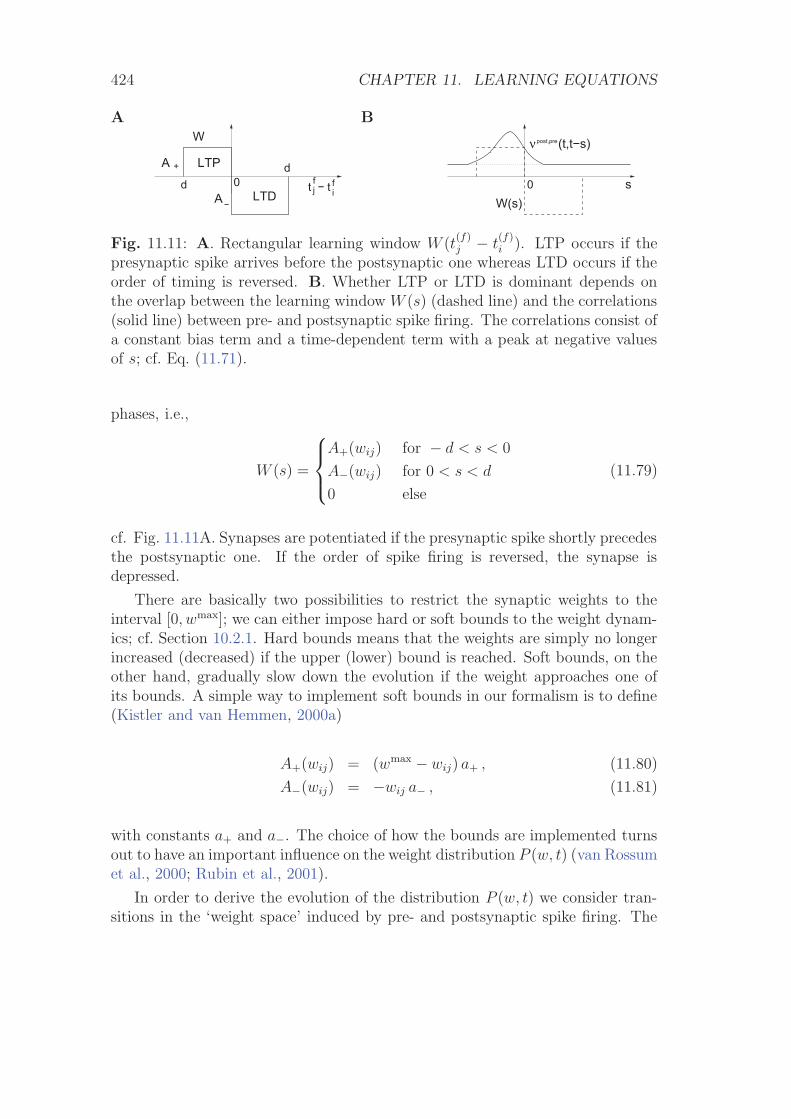
424 CHAPTER 11. LEARNING EQUATIONS
A B
fijftt −0d
+
−
A
A
d
LTD
LTP
W νpost,pre(t,t−s)
W(s)0 s
Fig. 11.11: A. Rectangular learning window W (t(f)j − t
(f)i ). LTP occurs if the
presynaptic spike arrives before the postsynaptic one whereas LTD occurs if theorder of timing is reversed. B. Whether LTP or LTD is dominant depends onthe overlap between the learning window W (s) (dashed line) and the correlations(solid line) between pre- and postsynaptic spike firing. The correlations consist ofa constant bias term and a time-dependent term with a peak at negative valuesof s; cf. Eq. (11.71).
phases, i.e.,
W (s) =
⎧⎪⎨⎪⎩
A+(wij) for − d < s < 0
A−(wij) for 0 < s < d
0 else
(11.79)
cf. Fig. 11.11A. Synapses are potentiated if the presynaptic spike shortly precedesthe postsynaptic one. If the order of spike firing is reversed, the synapse isdepressed.
There are basically two possibilities to restrict the synaptic weights to theinterval [0, wmax]; we can either impose hard or soft bounds to the weight dynam-ics; cf. Section 10.2.1. Hard bounds means that the weights are simply no longerincreased (decreased) if the upper (lower) bound is reached. Soft bounds, on theother hand, gradually slow down the evolution if the weight approaches one ofits bounds. A simple way to implement soft bounds in our formalism is to define(Kistler and van Hemmen, 2000a)
A+(wij) = (wmax − wij) a+ , (11.80)
A−(wij) = −wij a− , (11.81)
with constants a+ and a−. The choice of how the bounds are implemented turnsout to have an important influence on the weight distribution P (w, t) (van Rossumet al., 2000; Rubin et al., 2001).
In order to derive the evolution of the distribution P (w, t) we consider tran-sitions in the ‘weight space’ induced by pre- and postsynaptic spike firing. The
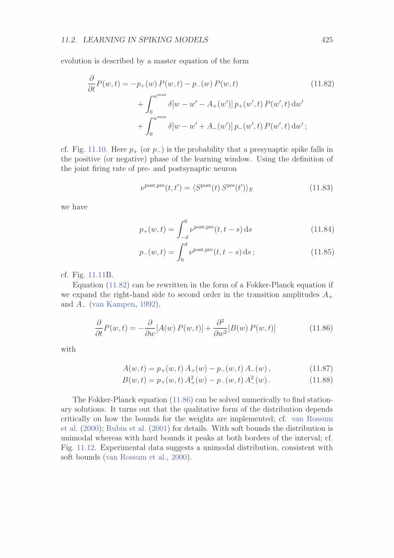
11.2. LEARNING IN SPIKING MODELS 425
evolution is described by a master equation of the form
∂
∂tP (w, t) = −p+(w) P (w, t)− p−(w) P (w, t) (11.82)
+
∫ wmax
0
δ[w − w′ − A+(w′)] p+(w′, t) P (w′, t) dw′
+
∫ wmax
0
δ[w − w′ + A−(w′)] p−(w′, t) P (w′, t) dw′ ;
cf. Fig. 11.10. Here p+ (or p−) is the probability that a presynaptic spike falls inthe positive (or negative) phase of the learning window. Using the definition ofthe joint firing rate of pre- and postsynaptic neuron
νpost,pre(t, t′) = 〈Spost(t) Spre(t′)〉E (11.83)
we have
p+(w, t) =
∫ 0
−d
νpost,pre(t, t− s) ds (11.84)
p−(w, t) =
∫ d
0
νpost,pre(t, t− s) ds ; (11.85)
cf. Fig. 11.11B.
Equation (11.82) can be rewritten in the form of a Fokker-Planck equation ifwe expand the right-hand side to second order in the transition amplitudes A+
and A− (van Kampen, 1992),
∂
∂tP (w, t) = − ∂
∂w[A(w) P (w, t)] +
∂2
∂w2[B(w) P (w, t)] (11.86)
with
A(w, t) = p+(w, t) A+(w)− p−(w, t) A−(w) , (11.87)
B(w, t) = p+(w, t) A2+(w)− p−(w, t) A2
−(w) . (11.88)
The Fokker-Planck equation (11.86) can be solved numerically to find station-ary solutions. It turns out that the qualitative form of the distribution dependscritically on how the bounds for the weights are implemented; cf. van Rossumet al. (2000); Rubin et al. (2001) for details. With soft bounds the distribution isunimodal whereas with hard bounds it peaks at both borders of the interval; cf.Fig. 11.12. Experimental data suggests a unimodal distribution, consistent withsoft bounds (van Rossum et al., 2000).
426 CHAPTER 11. LEARNING EQUATIONS
A BP
0
P (w)0
wmax w
P (w)0
P
0 wmax w
Fig. 11.12: Stationary distribution of synaptic weights. A. With soft bounds,the distribution of weights P0(w) has a single peak. B. With hard bounds, thedistribution peaks at the two boundaries w = 0 and w = wmax; (schematic figure)
11.3 Summary
The synaptic weight dynamics can be studied analytically if weights are changingslowly as compared to the time scale of the neuronal activity. We have seen thatweight changes are driven by correlations between pre- and postsynaptic activ-ity. More specifically, simple Hebbian learning rules can find the first principalcomponent of a normalized input data set. If non-Hebbian terms are includedthen both spike-based and rate-based learning rules can be constructed that arecharacterized by a stable fixed point for the sum of the synaptic weights. Thisfixed point leads to an intrinsic normalization of the output firing rate.
The interesting aspect of spike-time dependent plasticity is that it naturallyaccounts for temporal correlations in the input by means of a learning window.Explicit expressions for temporal spike-spike correlations can be obtained for cer-tain simple types of neuron model such as the linear Poisson model. In this case,correlations between pre- and postsynaptic neurons can be formulated in terms ofthe correlations in the input. It can be shown that, under certain circumstances,the weight vector evolves in the direction of the principal component of the inputpattern set, even if the input is not normalized.
Spike-based and rate-based rules of plasticity are equivalent as long as tempo-ral correlations are disregarded. The integral over the learning window
∫∞−∞W (s) ds
plays the role of the Hebbian correlation term ccorr2 . If rates vary rapidly, i.e. on
the time scale of the learning window, then spike-time dependent plasticity isdistinct from a rate-based formulation.
In addition to an analysis of the expectation value of the synaptic weightvector the distribution of weights can be described by means of a Fokker-Planckequation. The stationary distribution depends on the details of the learning rule.
References
More on the theory of unsupervised learning and principal component analysiscan be found in the classical book by Hertz et al. (1991). Models of the devel-opment of receptive fields and cortical maps have a long tradition in the field

11.3. SUMMARY 427
of computational neuroscience; see, e.g., von der Malsburg (1973); Sejnowski(1977); Kohonen (1984); Linsker (1986c); Sejnowski and Tesauro (1989); Milleret al. (1989); MacKay and Miller (1990); Shouval and Perrone (1995); Miller(1994); for a review see, e.g., Erwin et al. (1995); Wiskott and Sejnowski (1998).The linear rate model discussed in Section 11.1 is reviewed in Miller (1995). Theessential aspects of the weight dynamics in linear networks are discussed in Oja(1982); MacKay and Miller (1990); Miller and MacKay (1994).
The theory of spike-based Hebbian learning has been developed by Gerstneret al. (1996a); Hafliger et al. (1997); Ruf and Schmitt (1997); Eurich et al. (1999);Kempter et al. (1999); Roberts (1999, 2000); Roberts and Bell (2000); Kistler andvan Hemmen (2000b); van Rossum et al. (2000); Xie and Seung (2000); Song et al.(2000); Senn et al. (2001b); Rubin et al. (2001); and others. Spike-based learningrules are closely related to rules for sequence learning (Herz et al., 1988, 1989;van Hemmen et al., 1990; Gerstner et al., 1993b; Minai and Levy, 1993; Abbottand Blum, 1996; Gerstner and Abbott, 1997), where the idea of an asymmetriclearning windows is exploited.

428 CHAPTER 11. LEARNING EQUATIONS
Chapter 12
Plasticity and Coding
In Chapters 10 and 11 we have explored the principle of Hebbian synaptic plas-ticity. In this final chapter we would like to close the chain of arguments thatwe have followed across the book and establish a link between synaptic plasticityand the problems of neuronal coding and signal transmission. We will start thechapter with the question of rapid and reliable signal transmission, a questionthat we have encountered on several occasions in this book. In Section 12.1 wewill see that an asymmetric spike-time dependent learning rule is capable of de-tecting early events that may serve as predictors for others. Such a mechanismcan speed up signal processing and, hence, the reaction time. In Section 12.2we show that spike-time dependent plasticity can enhance signal transmissionby selectively stregthening synaptic connections that transmit precisely timedspikes at the expense of those synapses that transmit poorly timed spikes. InSection 12.3 we turn to sequence learning and explore whether spike-time depen-dent plasticity can support coding schemes that are based on spatio-temporalspike patterns with a millisecond resolution. The last two sections study codingproperties of specific neuronal systems. In Section 12.4 we will illustrate the roleof an inverted (or anti-)Hebb rule for the subtraction of expectations - which hasbeen hypothesized as an important component of signal processing in electric fish.Finally, in Section 12.5 we will see that a spike-time dependent Hebbian rule canplay an important role in the developmental tuning of signal transmission in theauditory system of barn owls.
12.1 Learning to be Fast
In many real-world situations we must react rapidly to the earliest signs thatcould warn us about harmful stimuli. If an obstacle blocks our way, we want toavoid it before a painful contact occurs. If we ride a bicycle, we should makecorrecting steering movements already at small inclination angles of the bicycle,well before we fall down. Spike-time dependent learning rules with a temporally
429
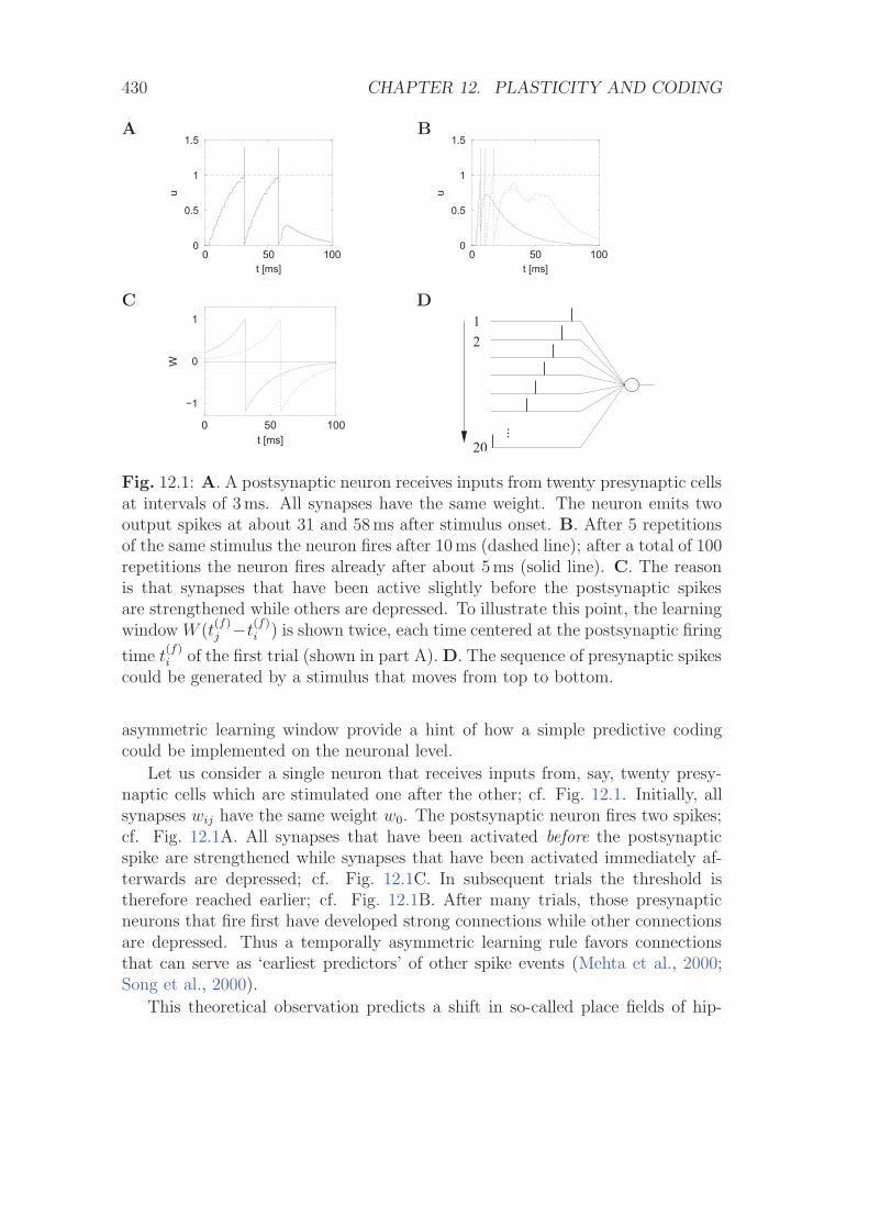
430 CHAPTER 12. PLASTICITY AND CODING
A B
0 50 100t [ms]
0
0.5
1
1.5
u
0 50 100t [ms]
0
0.5
1
1.5
u
C D
0 50 100t [ms]
−1
0
1
W
...
1
20
2
Fig. 12.1: A. A postsynaptic neuron receives inputs from twenty presynaptic cellsat intervals of 3ms. All synapses have the same weight. The neuron emits twooutput spikes at about 31 and 58ms after stimulus onset. B. After 5 repetitionsof the same stimulus the neuron fires after 10ms (dashed line); after a total of 100repetitions the neuron fires already after about 5ms (solid line). C. The reasonis that synapses that have been active slightly before the postsynaptic spikesare strengthened while others are depressed. To illustrate this point, the learningwindow W (t
(f)j −t
(f)i ) is shown twice, each time centered at the postsynaptic firing
time t(f)i of the first trial (shown in part A). D. The sequence of presynaptic spikes
could be generated by a stimulus that moves from top to bottom.
asymmetric learning window provide a hint of how a simple predictive codingcould be implemented on the neuronal level.
Let us consider a single neuron that receives inputs from, say, twenty presy-naptic cells which are stimulated one after the other; cf. Fig. 12.1. Initially, allsynapses wij have the same weight w0. The postsynaptic neuron fires two spikes;cf. Fig. 12.1A. All synapses that have been activated before the postsynapticspike are strengthened while synapses that have been activated immediately af-terwards are depressed; cf. Fig. 12.1C. In subsequent trials the threshold istherefore reached earlier; cf. Fig. 12.1B. After many trials, those presynapticneurons that fire first have developed strong connections while other connectionsare depressed. Thus a temporally asymmetric learning rule favors connectionsthat can serve as ‘earliest predictors’ of other spike events (Mehta et al., 2000;Song et al., 2000).
This theoretical observation predicts a shift in so-called place fields of hip-
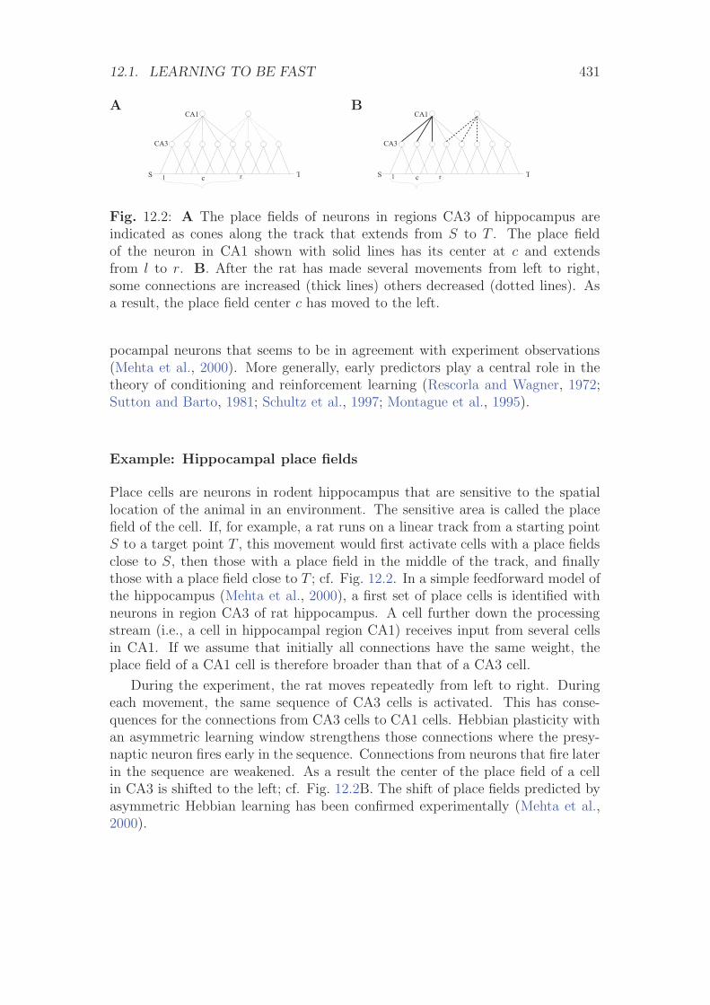
12.1. LEARNING TO BE FAST 431
A B
CA3
CA1
S Tcl r
CA3
CA1
S Tl c r
Fig. 12.2: A The place fields of neurons in regions CA3 of hippocampus areindicated as cones along the track that extends from S to T . The place fieldof the neuron in CA1 shown with solid lines has its center at c and extendsfrom l to r. B. After the rat has made several movements from left to right,some connections are increased (thick lines) others decreased (dotted lines). Asa result, the place field center c has moved to the left.
pocampal neurons that seems to be in agreement with experiment observations(Mehta et al., 2000). More generally, early predictors play a central role in thetheory of conditioning and reinforcement learning (Rescorla and Wagner, 1972;Sutton and Barto, 1981; Schultz et al., 1997; Montague et al., 1995).
Example: Hippocampal place fields
Place cells are neurons in rodent hippocampus that are sensitive to the spatiallocation of the animal in an environment. The sensitive area is called the placefield of the cell. If, for example, a rat runs on a linear track from a starting pointS to a target point T , this movement would first activate cells with a place fieldsclose to S, then those with a place field in the middle of the track, and finallythose with a place field close to T ; cf. Fig. 12.2. In a simple feedforward model ofthe hippocampus (Mehta et al., 2000), a first set of place cells is identified withneurons in region CA3 of rat hippocampus. A cell further down the processingstream (i.e., a cell in hippocampal region CA1) receives input from several cellsin CA1. If we assume that initially all connections have the same weight, theplace field of a CA1 cell is therefore broader than that of a CA3 cell.
During the experiment, the rat moves repeatedly from left to right. Duringeach movement, the same sequence of CA3 cells is activated. This has conse-quences for the connections from CA3 cells to CA1 cells. Hebbian plasticity withan asymmetric learning window strengthens those connections where the presy-naptic neuron fires early in the sequence. Connections from neurons that fire laterin the sequence are weakened. As a result the center of the place field of a cellin CA3 is shifted to the left; cf. Fig. 12.2B. The shift of place fields predicted byasymmetric Hebbian learning has been confirmed experimentally (Mehta et al.,2000).
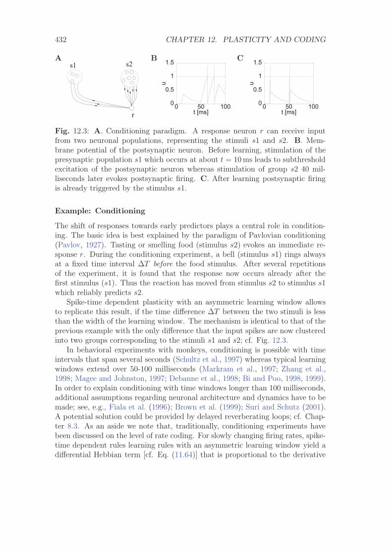
432 CHAPTER 12. PLASTICITY AND CODING
A B C
r
s1 s2
0 50 100t [ms]
0
0.5
1
1.5
u
0 50 100t [ms]
0
0.5
1
1.5
u
Fig. 12.3: A. Conditioning paradigm. A response neuron r can receive inputfrom two neuronal populations, representing the stimuli s1 and s2. B. Mem-brane potential of the postsynaptic neuron. Before learning, stimulation of thepresynaptic population s1 which occurs at about t = 10 ms leads to subthresholdexcitation of the postsynaptic neuron whereas stimulation of group s2 40 mil-liseconds later evokes postsynaptic firing. C. After learning postsynaptic firingis already triggered by the stimulus s1.
Example: Conditioning
The shift of responses towards early predictors plays a central role in condition-ing. The basic idea is best explained by the paradigm of Pavlovian conditioning(Pavlov, 1927). Tasting or smelling food (stimulus s2) evokes an immediate re-sponse r. During the conditioning experiment, a bell (stimulus s1) rings alwaysat a fixed time interval ΔT before the food stimulus. After several repetitionsof the experiment, it is found that the response now occurs already after thefirst stimulus (s1). Thus the reaction has moved from stimulus s2 to stimulus s1which reliably predicts s2.
Spike-time dependent plasticity with an asymmetric learning window allowsto replicate this result, if the time difference ΔT between the two stimuli is lessthan the width of the learning window. The mechanism is identical to that of theprevious example with the only difference that the input spikes are now clusteredinto two groups corresponding to the stimuli s1 and s2; cf. Fig. 12.3.
In behavioral experiments with monkeys, conditioning is possible with timeintervals that span several seconds (Schultz et al., 1997) whereas typical learningwindows extend over 50-100 milliseconds (Markram et al., 1997; Zhang et al.,1998; Magee and Johnston, 1997; Debanne et al., 1998; Bi and Poo, 1998, 1999).In order to explain conditioning with time windows longer than 100 milliseconds,additional assumptions regarding neuronal architecture and dynamics have to bemade; see, e.g., Fiala et al. (1996); Brown et al. (1999); Suri and Schutz (2001).A potential solution could be provided by delayed reverberating loops; cf. Chap-ter 8.3. As an aside we note that, traditionally, conditioning experiments havebeen discussed on the level of rate coding. For slowly changing firing rates, spike-time dependent rules learning rules with an asymmetric learning window yield adifferential Hebbian term [cf. Eq. (11.64)] that is proportional to the derivative
Bibliography
Abbott, L. F. (1991). Realistic synaptic inputs for model neural networks. Net-work, 2:245–258. 68
Abbott, L. F. (1994). Decoding neuronal firing and modeling neural networks.Quart. Rev. Biophys., 27:291–331. 34, 38
Abbott, L. F. (2000). Synaptic plastictiy - taming the beast. Nature Neurosci.,3:1178–1183. 394
Abbott, L. F. and Blum, K. I. (1996). Functional significance of long-term po-tentiation for sequence learning and prediction. Cereb. Cortex, 6:406–416. 427
Abbott, L. F., Fahri, E., and Gutmann, S. (1991). The path integral for dendritictrees. Biol. Cybern., 66:49–60. 71, 143
Abbott, L. F. and Kepler, T. B. (1990). Model neurons: from Hodgkin-Huxleyto Hopfield. In Garrido, L., editor, Statistical Mechanics of Neural Networks.Springer, Berlin. 80, 99
Abbott, L. F. and van Vreeswijk, C. (1993). Asynchronous states in a networkof pulse-coupled oscillators. Phys. Rev. E, 48:1483–1490. 105, 107, 213, 217,229, 231, 256, 295
Abeles, M. (1982). Local cortical circuits. Springer-Verlag, Berlin Heidelberg NewYork. 176, 177
Abeles, M. (1991). Corticonics. Cambridge Univ. Press, Cambridge. 32, 111,194, 195, 291, 351, 357, 441
Abeles, M. (1994). Firing rates and well-timed events. In Domany, E., Schulten,K., and van Hemmen, J. L., editors, Models of Neural Networks II, chapter 3.Springer, New York. 24, 32, 38
Abeles, M., Bergman, H., Margalit, E., and Vaadia, E. (1993). Spatiotemporalfiring patterns in the frontal cortex of behaving monkeys. J. Neurophysiol.,70:1629–1638. 32
463
464 BIBLIOGRAPHY
Adrian, E. D. (1926). The impulses produced by sensory nerve endings. J.Physiol. (Lond.), 61:49–72. 24, 25
Adrian, E. D. (1928). The basis of sensation. W. W. Norton, New York. 24
Aertsen, A. and Arndt, M. (1993). Response synchronization in the visual cortex.Curr. Opin. Neurobiol., 3:586–594. 32
Aizenman, C. D. and Linden, D. J. (1999). Regulation of the rebound depolar-ization and spontaneous firing patterns of deep nuclear neurons in slices of ratcerebellum. J. Neurophysiol., 82:1697–1709. 56
Amari, S. (1972). Characteristics of random nets of analog neuron-like elements.IEEE trans. syst. man cybern., 2:643–657. 246, 248, 256
Amari, S. (1974). A method of statistical neurodynamics. Kybernetik, 14:201–215.213, 246, 256
Amari, S. (1977a). Dynamics of pattern formation in lateral-inhibition type neuralfields. Biol. Cybern., 27:77–87. 254, 256
Amari, S. I. (1977b). Dynamics of pattern formation in lateral-inhibition typeneural fields. Biol. Cybern., 27:77–87. 246, 256, 325, 334, 341
Amit, D. J. and Brunel, N. (1997a). Model of global spontaneous activity andlocal structured activity during delay periods in the cerebral cortex. Cereb.Cortex, 7:237–252. 188, 213, 246, 248, 250, 256
Amit, D. J. and Brunel, N. (1997b). A model of spontaneous activity and localdelay activity during delay periods in the cerebral cortex. Cerebral Cortex,7:237–252. 213, 246, 248, 250
Anderson, J. A. and Rosenfeld, E., editors (1988). Neurocomputing: Foundationsof research. MIT-Press, Cambridge Mass. 209, 393
Artola, A., Brocher, S., and Singer, W. (1990). Different voltage dependentthresholds for inducing long-term depression and long-term potentiation inslices of rat visual cortex. Nature, 347:69–72. 371
Artola, A. and Singer, W. (1993). Long-term depression of excitatory synaptictransmission and its relationship to long-term potentiation. Trends Neurosci.,16(11):480–487. 371, 394
Ash, R. (1990). Information Theory. Dover, New York. 320
BIBLIOGRAPHY 465
Bair, W. and Koch, C. (1996). Temporal precision of spike trains in extrastriatecortex of the behaving macaque monkey. Neural Comput., 8:1185–1202. 157,158, 159, 209
Bair, W., Koch, C., Newsome, W., and Britten, K. (1994). Power spectrumanalysis of MT neurons in the behaving monkey. J. Neurosci., 14:2870–2892.170, 172, 173
Bartlett, M. S. (1963). The spectral analysis of point processes. J. R. Statist.Soc. B, 25:264–296. 416, 435
Bauer, H. U. and Pawelzik, K. (1993). Alternating oscillatory and stochasticdynamics in a model for a neuronal assembly. Physica D, 69:380–393. 217
Bell, C., Bodznick, D., Montgomery, J., and Bastian, J. (1997a). The generationand subtraction of sensory expectations within cerebellar-like structures. Brain.Beh. Evol., 50:17–31. suppl. I. 446, 448
Bell, C., Han, V., Sugawara, Y., and Grant, K. (1997b). Synaptic plasticity ina cerebellum-like structure depends on temporal order. Nature, 387:278–281.366, 393, 446, 447, 449
Bell, C. C. and Kawasaki, T. (1972). Relations among climbing fiber responsesof nearby Purkinje cells. J. Neurophysiol., 35:155–169. 311
Ben Arous, G. and Guionnet, A. (1995). Large deviations for langevin spin glassdynamics. Probability Theory and Related Fields, 102:455–509. 248
Ben-Yishai, R., Lev Bar-Or, R., and Sompolinsky, H. (1995). Theory of ori-entation tuning in visual cortex. Proc. Natl. Acad. Sci. USA, 92:3844–3848.334
Berry, M. J. and Meister, M. (1998). Refractoriness and neural precision. J.Neurosci., 18:2200–2211. 169, 179
Berry, M. J., Warland, D. K., and Meister, M. (1997). The structure and precisionof retinal spike trains. Proc. Natl. Acad. Sci. USA, 94:5411–5416. 157, 159
Bethge, M., Pawelzik, K., Rothenstein, R., and Tsodyks, M. (2001). Noise as asignal for neuronal populations. Phys. Rev. Lett., xx:xx. 259
Bi, G. and Poo, M. (1998). Synaptic modifications in cultured hippocampalneurons: dependence on spike timing, synaptic strength, and postsynaptic celltype. J. Neurosci., 18:10464–10472. 365, 366, 393, 432, 449
Bi, G. and Poo, M. (2001). Synaptic modification of correlated activity: Hebb’spostulate revisited. Ann. Rev. Neurosci., 24:139–166. 365, 369, 394
466 BIBLIOGRAPHY
Bi, G. Q. and Poo, M. M. (1999). Distributed synaptic modification in neuralnetworks induced by patterned stimulation. Nature, 401:792–796. 365, 366,393, 432
Bialek, W. and Rieke, F. (1992). Reliability and information transmission inspiking neurons. Trends Neurosci., 15(11):428–433. 34
Bialek, W., Rieke, F., de Ruyter van Stevenick, R. R., and Warland, D. (1991).Reading a neural code. Science, 252:1854–1857. 24, 33, 34, 36, 159
Bienenstock, E. L., Cooper, L. N., and Munroe, P. W. (1982). Theory of the devel-opment of neuron selectivity: orientation specificity and binocular interactionin visual cortex. J. Neurosci., 2:32–48. reprinted in Anderson and Rosenfeld,1990. 371, 386, 393
Billock, V. A. (1997). Very short-term visual memory via reverberation: a rolefor the cortico-thalamic excitatory circuit in temporal filling-in during blinksand saccades? Vision Res., 37:949–953. 312, 320
Bindman, L., Christofi, G., Murphy, K., and Nowicky, A. (1991). Long-termpotentiation (ltp) and depression (ltd) in the neocortex and hippocampus: anoverview. In TW, S., editor, Aspects of synaptic transmission., volume 1, pages3–25, London. Taylor Francis. 387
Bliss, T. V. P. and Collingridge, G. L. (1993). A synaptic model of memory:long-term potentiation in the hippocampus. Nature, 361:31–39. 362, 363, 387,394
Bliss, T. V. P. and Gardner-Medwin, A. R. (1973). Long-lasting potentation ofsynaptic transmission in the dendate area of unanaesthetized rabbit followingstimulation of the perforant path. J. Physiol., 232:357–374. 362
Bliss, T. V. P. and Lomo, T. (1973). Long-lasting potentation of synaptic trans-mission in the dendate area of anaesthetized rabbit following stimulation of theperforant path. J. Physiol., 232:551–356. 362
Bose, A., Kopell, N., and Terman, D. (2000). Almost-synchronous solutions formutually coupled excitatory neurons. Physica D, 140:69–94. 301
Bower, J. M. and Beeman, D. (1995). The Book of GENESIS: exploring realisticneural models with the GEneral NEural SImulation System. Springer, NewYork. 71, 72, 76
Bressloff, P. C. (1999). Synaptically generated wave propagation in excitableneural media. Phys. Rev. Lett., 82:2979–2982. 345, 347
BIBLIOGRAPHY 467
Bressloff, P. C. and Taylor, J. G. (1994). Dynamics of compartmental modelneurons. Neural Networks, 7:1153–1165. 143, 146
Brillinger, D. R. (1988). Maximum likelihood analysis of spike trains of interactingnerve cells. Biol. Cybern., 59:189–200. 119, 155
Brillinger, D. R. (1992). Nerve cell spike train data analysis: a progressiion ofthechniques. J. Am. Statist. Assoc., 87:260–271. 119, 155
Brillinger, D. R. and Segundo, J. P. (1979). Empirical examination of the thresh-old model of neuronal firing. Biol. Cybern., 35:213–220. 119
Brown, J., Bullock, D., and Grossberg, S. (1999). How the basal ganglia useparallel excitatory and inhibitory learning pathways to selectively respond tounexpected rewarding cues. J. Neurosci., 19:10502–11. 432
Brown, T. H., Ganong, A. H., Kairiss, E. W., Keenan, C. L., and Kelso, S. R.(1989). Long-term potentiation in two synaptic systems of the hippocampalbrain slice. In JH, B. and WO, B., editors, Neural models of plasticity., pages266–306. Academic Press, San Diego. 362, 363, 394
Brown, T. H., Zador, A. M., Mainen, Z. F., and Claiborne, B. J. (1991). Hebbianmodifications in hippocampal neurons. In Baudry, M. and Davis, J. L., editors,Long-term potentiation., pages 357–389. MIT Press, Cambridge, London. 366,369
Brunel, N. (2000). Dynamics of sparsely connected networks of excitatory andinhibitory spiking neurons. J. Comput. Neurosci., 8:183–208. 213, 246, 248,250, 256, 296, 299, 300
Brunel, N., Chance, F., Fourcaud, N., and Abbott, L. F. (2001). Effects ofsynaptic noise and filtering on the frequency response of spiking neurons. Phys.Rev. Lett., 86:2186–2189. 28, 259, 273, 276, 277, 279, 280, 290, 291
Brunel, N. and Hakim, V. (1999). Fast global oscillations in networks of integrate-and-fire neurons with low firing rates. Neural Comput., 11:1621–1671. 160,188, 213, 217, 222, 246, 250, 254, 255, 256, 259, 296, 299
Bryant, H. L. and Segundo, J. P. (1976). Spike initiation by transmembranecurrent: a white-noise analysis. J. Physiol. (Lond.), 260:279–314. 157, 159,287
Buck, J. and Buck, E. (1976). Synchronous fireflies. Sci. Am., 234:74–85. 322
Bugmann, G., Christodoulou, C., and Taylor, J. G. (1997). Role of temporalintegration and fluctuation detection in the highly irregular firing of leaky in-tegrator neuron model with partial reset. Neural Comput., 9:985–1000. 195
468 BIBLIOGRAPHY
Burkitt, A. N. and Clark, G. M. (1999). Analysis of integrate-and-fire neurons:synchronization of synaptic input and spike output. Neural Comput., 11:871–901. 194
Byrne, J. H. and Berry, W. O. (1989). Neural Models of Plasticity. AcademicPress, San Diego. 394
Calvin, W. and Stevens, C. F. (1968). Synaptic noise and other sources of ran-domness in motoneuron interspike intervals. J. Neurophysiol., 31:574–587. 222
Capocelli, R. M. and Ricciardi, L. M. (1971). Diffusion approximation and firstpassage time problem for a neuron model. Kybernetik, 8:214–223. 188
Carpenter, G. and Grossberg, S. (1987). Art 2: Self-organization of stable cate-gory recognition codes for analog input patterns. Appl. Optics, 26:4919–4930.376
Carr, C. E. (1993). Processing of temporal information in the brain. Annu. Rev.Neurosci., 16:223–243. 372, 450, 455, 456, 462
Carr, C. E. (1995). The development of nucleus laminaris in the barn owl. InManley, G. A., Klump, G. M., Koppl, C., Fastl, H., and Oeckinghaus, H., edi-tors, Advances in Hearing Research, pages 24–30, Singapure. World Scientific.450, 457, 461
Carr, C. E. and Konishi, M. (1988). Axonal delay lines for measurement in theowl’s brainstem. Proc. Natl. Acad. Sci. USA, 85:8311–8315. 450
Carr, C. E. and Konishi, M. (1990). A circuit for detection of interaural timedifferences in the brain stem of the barn owl. J. Neurosci., 10:3227–3246. 372,450, 452, 455, 456, 457
Cessac, B., Doyon, B., Quoy, M., and Samuelides, M. (1994). Mean-field equa-tions, bifurcation map and route to chaos in discrete time neural networks.Physica D, 74:24–44. 246, 248, 256
Chow, C. C. (1998). Phase-locking in weakly heterogeneous neuronal networks.Physica D, 118:343–370. 254, 301, 309
Chow, C. C. and Kopell, N. (2000). Dynamics of spiking neurons with electricalcoupling. Neural Comput., 12:1643–1678. 301
Chow, C. C. and White, J. (1996). Spontaneous action potential fluctuations dueto channel fluctuations. Bioph. J., 71:3013–3021. 160
BIBLIOGRAPHY 469
Collingridge, G. L., Kehl, S. J., and McLennan, H. (1983). Excitatory aminoacids in synaptic transmission in the schaffer collateral-commissural pathwayof the rat hippocampus. J. Physiol., 334:33–46. 387
Collins, J. J., Chow, C. C., Capela, A. C., and Imhoff, T. T. (1996). Aperiodicstochastic resonance. Phys. Rev. E, 54:5575–5584. 201
Connor, J. A., Walter, D., and McKown, R. (1977). Neural repetitive firing -modifications of the hodgkin-huxley axon suggested by experimental resultsfrom crustacean axons. Biophys. J., 18:81–102. 54
Connors, B. W. and Gutnick, M. J. (1990). Intrinsic firing patterns of diversecortical neurons. Trends Neurosci., 13:99–104. 19, 20, 255
Cordo, P., Inglis, J. T., Verschueren, S., andD. M. Merfeld, J. J. C., and Rosen-blum, S. (1996). Noise in human muscle spindels. Nature, 383:769–770. 201
Cover, T. M. and Thomas, J. A. (1991). Elements of Information Theory. Wiley,New York. 320
Cox, D. R. (1955). Some statistical methods connected with series of events. J.R. statist. Soc. B, 17:129–164. 416, 435
Cox, D. R. (1962). Renewal theory. Mathuen, London. 161, 164, 255
Cox, D. R. and Lewis, P. A. W. (1966). The statistical analysis of series of events.Methuen, London. 164, 172, 209
Crepel, F. (1982). Regression of functional synapses in the immature mammaliancerebellum. Trends Neurosci., 5:266–269. 376
Crisanti, A. and Sompolinsky, H. (1988). Dynamics of spin systems with randomlyasymmetric bonds: Ising spins and Glauber dynamics. Phys. Rev. A, 37:4865–4874. 246, 314
Cronin, J. (1987). Mathematical aspects of Hodgkin-Huxley theory. CambridgeUniversity Press, Cambridge.
Daniel, H., Blond, O., Jaillard, D., and Crepel, F. (1996). Synaptic plasticityin the cerebellum. In Fazeli, M. S. and Collingridge, G. L., editors, CorticalPlasticity, LTP and LTD, chapter 10. BIOS Scientific Publishers Ltd., Oxford.394
Daniel, H., Levenes, C., and Crepel, F. (1998). Cellular mechanisms of cerebellarLTD. Trends Neurosci., 21:401–407. 394
470 BIBLIOGRAPHY
de Boer, E. and Kuyper, P. (1968). Triggered correlation. IEEE Trans. Biomed.Eng., 15:169–179. 32
de Ruyter van Stevenick, R. R. and Bialek, W. (1988). Real-time performanceof a movement-sensitive neuron in the blowfly visual system: coding and in-formation transfer in short spike sequences. Proc. R. Soc. B, 234:379–414.33
de Ruyter van Steveninck, R. R., Lowen, G. D., Strong, S. P., Koberle, R.,and Bialek, W. (1997). Reproducibility and variability in neural spike trains.Science, 275:1805. 157, 159
De Zeeuw, C. I., Simpson, J. I., Hoogenraad, C. C., Galjart, N., Koekkoek, S.K. E., and Ruigrok, T. J. H. (1998). Microcircuitry and function of the inferiorolive. Trends Neurosci., 21:391–400. 311
DeAngelis, G. C., Ohzwaw, I., and Freeman, R. D. (1995). Receptive-field dy-namics in the central visual pathways. Trends Neurosci., 18:451–458. 33
Debanne, D., Gahwiler, B. H., and Thompson, S. M. (1994). Asynchronous pre-and postsynaptic activity induces associative long-term depression in area CA1of the rat Hippocampus in vitro. Proc. Natl. Acad. Sci. USA, 91:1148–1152.364
Debanne, D., Gahwiler, B. H., and Thompson, S. M. (1998). Long-term synapticplasticity between pairs of individual CA3 pyramidal cells in rat hippocampalslice cultures. J. Physiol., 507:237–247. 365, 366, 393, 432, 449
deCharms, R. C. and Merzenich, M. M. (1996). Primary cortical representationof sounds by the coordination of action-potential timing. Nature, 381:610–613.32
Derrida, B., Gardner, E., and Zippelius, A. (1987). An exactly solvable asym-metric neural network model. Europhys. Lett., 2:167–173. 247, 314
Desmaison, D., Vincent, J.-D., and Lledo, P.-M. (1999). Control of action po-tential timing by intrinsic subthreshold oscillations in olfactory bulb outputneurons. J. Neurosci., 19:10727–10737. 293
Destexhe, A. and Pare, D. (1999). Impact of network activity on the integrativeproperties of neocortical pyramidal neurons in vivo. J. Neurophysiol., 81:1531–1547. 222
Diesmann, M., Gewaltig, M.-O., and Aertsen, A. (1999). Stable propagation ofsynchronous spiking in cortical neural networks. Nature, 402:529–533. 351,353, 356
BIBLIOGRAPHY 471
Douglass, J. K., Wilkens, L., Pantazelou, E., and Moss, F. (1993). Noise en-hancement of information transfer in crayfish mechanoreceptors by stochasticresonance. Nature, 365:337–340. 201
Dudek, S. M. and Bear, M. F. (1992). Homosynaptic long-term depression inarea ca1 of hippocampus and effects of n-methyl-d-aspartate receptor blockade.Proc. Natl. Acad. Sci. USA, 89:4363–4367. 387
Eckhorn, R., Bauer, R., Jordan, W., Brosch, M., Kruse, W., Munk, M., andReitboeck, H. J. (1988). Coherent oscillations: A mechanism of feature linkingin the visual cortex? Biol. Cybern., 60:121–130. 24, 32, 293
Eckhorn, R. and Brosch, M. (1993). Synchronous oscillatory activities betweenareas 17 and 18 in the cat’s visual cortex. J. Neurophysiol. in press. 293
Eckhorn, R., Krause, F., and Nelson, J. L. (1993). The rf-cinematogram: a cross-correlation technique for mapping several visual fields at once. Biol. Cybern.,69:37–55. 33
Eckhorn, R., Reitboeck, H. J., Arndt, M., and Dicke, P. (1990). Feature linkingvia synchronization among distributed assemblies: Simulations of results fromcat visual cortex. Neural Comput., 2:293–307. 32, 111
Edwards, B. E. and Wakefield, G. H. (1993). The spectral shaping of neuraldischarges by refractory effects. J. Acoust. Soc. Am., 93:3553–3564. 170, 172,173
Egger, V., Feldmeyer, D., and Sakmann, B. (1999). Coincidence detection andchanges of synaptic efficacy in spiny stellate neurons in barrel cortex. NatureNeurosci., 2:1098–1105. 366, 393
Eggert, J. and van Hemmen, J. L. (2001). Modeling neuronal assemblies: theoryand implementation. Neural Computation, 13:1923–1974. 213
Ekeberg, O., Wallen, P., Lansner, A., Traven, H., Brodin, L., and Grillner, S.(1991). A computer based model for realistic simulations of neural networks.Biol. Cybern., 65:81–90. 71
Ellias, S. A. and Grossberg, S. (1975). Pattern formation, contrast control, andoscillations in the short term memory of shunting on-center off-surround net-works. Biol. Cybern., 20:69–98. 254, 256
Engel, A. K., Konig, P., Kreiter, A. K., and Singer, W. (1991a). Interhemisphericsynchronization of oscillatory neural responses in cat visual cortex. Science,252:1177–1179. 24, 32
472 BIBLIOGRAPHY
Engel, A. K., Konig, P., and Singer, W. (1991b). Direct physiological evidence forscene segmentation by temporal coding. Proc. Natl. Acad. Sci. USA, 88:9136–9140. 32
Erisir, A., Lau, D., Rudy, B., and Leonard, C. S. (1999). Specific k+ channels arerequired to sustain high frequency firing in fast-spiking neocortical interneu-rons. J. Neurophysiol., 82:2476–2489. 54, 132
Ermentrout, G. B. (1996). Type i membranes, phase resetting curves, and syn-chrony. Neural Comput., 8:979–1001. 91, 99, 106, 107, 132, 301
Ermentrout, G. B. and Cowan, J. D. (1979). A mathematical theory of visualhallucination patterns. Biol. Cybern., 34:137–150. 357
Ermentrout, G. B. and Kopell, N. (1984). Frequency plateaus in a chain of weaklycoupled oscillators. SIAM J. Math. Anal., 15:215–237. 301
Ermentrout, G. B. and Kopell, N. (1986). Parabolic bursting in an excitablesystem coupled with a slow oscillation. SIAM J. Appl. Math., 46:233–253. 107
Ermentrout, G. B., Pascal, M., and Gutkin, B. (2001). The effects of spikefrequency adaptation and negative feedback on the synchronization of neuronaloscillators. Neural Comput., 13:1285–1310. 301
Ernst, U., Pawelzik, K., and Geisel, T. (1995). Synchronization induced by tem-poral delays in pulse-coupled oscillators. Phys. Rev. Lett., 74:1570–1573. 296,301, 310
Erwin, E., Obermayer, K., and Schulten, K. (1995). Models of orientation andocular dominance columns in the visual cortex: a critcal comparison. NeuralComput., 7:425–468. 393, 427
Eurich, C. W., Pawelzik, K., Ernst, U., Cowan, J. D., and Milton, J. G. (1999).Dynamics of self-organized delay adaption. Phys. Rev. Lett., 82:1594–1597.427, 450, 457
Feldman, J. L. and Cowan, J. D. (1975). Large-scale activity in neural nets i:Theory with application to motoneuron pool responses. Biol. Cybern., 17:29–38. 254, 325
Feng, J. (2001). Is the integrate-and-fire model good enough - a review. NeuralComput., 13:xx. 106, 195
Fetz, E. E. and Gustafsson, B. (1983). Relation between shapes of post-synapticpotentials and changes in firing probability of cat motoneurones. J. Physiol.,341:387–410. 281, 282, 284, 285, 291
BIBLIOGRAPHY 473
Fiala, J., Grossberg, S., and Bullock, D. (1996). Metabotropic glutamate receptoractivation in cerebellar purkinje cells as a substrate for adaptive timing of theclassically conditioned eye-blink reflex. J. Neurosci., 16:3760–3774. 432
FitzHugh, R. (1961). Impulses and physiological states in models of nerve mem-brane. Biophys. J., 1:445–466. 79
French, A. S. and Stein, R. B. (1970). A flexible neural analog using integratedcircuits. IEEE trans. biomed. eng., 17(3):248–253. 155
Fuortes, M. G. F. and Mantegazzini, F. (1962). Interpretation of the repetitivefiring of nerve cells. J. Gen. Physiol., 45:1163–1179. 50, 111, 112, 113
Fusi, S., Del Giudice, P., and Amit, D. J. (2000). Neurophysiology of a vlsi spikingneural network: Lann21. In Proceedings of IJCNN2000. 160, 376, 380
Fusi, S. and Mattia, M. (1999). Collective behavior of networks with linear (vlsi)integrate and fire neurons. Neural Comput., 11:633–652. 213, 217
Gabbiani, F. and Koch, C. (1998). Principles of spike train analysis. In Koch, C.and Segev, I., editors, Methods in Neuronal Modeling, chapter 9, pages 312–360.MIT press, 2nd edition. 209
Gabbiani, F., Midtgaard, J., and Knoepfl, T. (1994). Synaptic integration in amodel of cerebellar granule cells. J. Neurophysiol., 72:999–1009. Corrigendahave been published in J. Neurophysiol. (1996) 75(6), without covering, how-ever, all typing errors. 62, 63, 72
Gamble, E. and Koch, C. (1987). The dynamics of free calcium in dendritic spinesin response to repetitive synaptic input. Science, 236:1311–1315. 389
Gammaitoni, L., Hanggi, P., Jung, P., and Marchesoni, F. (1998). Stochasticresonance. Rev. Mod. Phys., 70:223–287. 201, 209
Geisler, C. D. and Goldberg, J. M. (1966). A stochastic model of repetitiveactivity of neurons. Biophys. J., 6:53–69. 17, 38, 111, 155, 177, 209
Georgopoulos, A. P., Schwartz, A., and Kettner, R. E. (1986). Neuronal popula-tions coding of movement direction. Science, 233:1416–1419. 29
Gerstein, G. L. and Perkel, D. H. (1972). Mutual temporal relations amongneuronal spike trains. Biophys. J., 12:453–473. 164, 209
Gerstner, W. (1995). Time structure of the activity in neural network models.Phys. Rev. E, 51:738–758. 17, 111, 161, 213, 232, 238, 255, 296
474 BIBLIOGRAPHY
Gerstner, W. (1998). Spiking neurons. In Maass, W. and Bishop, C. M., editors,Pulsed Neural Networks, chapter 1, pages 3–53. MIT-Press. 150, 151
Gerstner, W. (2000a). Population dynamics of spiking neurons: fast transients,asynchronous states and locking. Neural Comput., 12:43–89. 28
Gerstner, W. (2000b). Population dynamics of spiking neurons: fast transients,asynchronous states, and locking. Neural Comput., 12:43–89. 124, 161, 182,213, 233, 240, 255, 259, 263, 270, 277, 278, 279, 290, 291, 296, 298
Gerstner, W. and Abbott, L. F. (1997). Learning navigational maps throughpotentiation and modulation of hippocampal place cells. J. Comput. Neurosci.,4:79–94. 427
Gerstner, W., Kempter, R., and van Hemmen, J. L. (1998). Hebbian learning ofpulse timing in the barn owl auditory system. In Maass, W. and Bishop, C. M.,editors, Pulsed Neural Networks, chapter 14, pages 353–377. MIT-Press. 382,383, 451, 454
Gerstner, W., Kempter, R., van Hemmen, J. L., and Wagner, H. (1996a). Aneuronal learning rule for sub-millisecond temporal coding. Nature, 386:76–78.383, 427, 442, 450, 456, 457, 458, 459
Gerstner, W., Kempter, R., van Hemmen, J. L., and Wagner, H. (1997). Adevelopmental learning rule for coincidence tuning in the barn owl auditorysystem. In Bower, J., editor, Computational Neuroscience: trends in research1997, pages 665–669. Plenum Press, New York. 450, 460
Gerstner, W., Ritz, R., and van Hemmen, J. L. (1993a). A biologically motivatedand analytically soluble model of collective oscillations in the cortex: I. theoryof weak locking. Biol. Cybern., 68:363–374. 32, 301
Gerstner, W., Ritz, R., and van Hemmen, J. L. (1993b). Why spikes? Heb-bian learning and retrieval of time-resolved excitation patterns. Biol. Cybern.,69:503–515. 427, 441, 442, 444
Gerstner, W. and van Hemmen, J. L. (1992). Associative memory in a networkof ‘spiking’ neurons. Network, 3:139–164. 213, 217, 226, 232
Gerstner, W. and van Hemmen, J. L. (1993). Coherence and incoherence in aglobally coupled ensemble of pulse emitting units. Phys. Rev. Lett., 71:312–315.296
Gerstner, W. and van Hemmen, J. L. (1994). Coding and information processingin neural networks. In Domany, E., van Hemmen, J. L., and Schulten, K.,editors, Models of Neural Networks II. Springer, New York. 217
BIBLIOGRAPHY 475
Gerstner, W., van Hemmen, J. L., and Cowan, J. D. (1996b). What matters inneuronal locking. Neural Comput., 8:1653–1676. 119, 123, 301, 303, 305
Gestri, G. (1978). Dynamics of a model for the variability of the interspikeintervals in a retinal neuron. Biol. Cybern., 31:97–98. 182
Gewaltig, M.-O. (2000). Evolution of synchronous spike volleys in cortical net-works – Network simulations and continuous probabilistic models. Shaker Ver-lag, Aachen, Germany. PhD thesis. 351, 353
Giorno, V., Nobile, A. G., and M.Ricciardi, L. (1992). Instantaneous returnprocesses and neuronal firings. In Trappl, R., editor, Cybernetics and SystemsResearch, Vol 1., pages 829–236. World Scientific Press. 222
Gluss, B. (1967). A model of neuron firing with exponential decay of potential re-sulting in diffusion equations for the probability density. Bull. Math. Biophys.,29:233–243. 188, 209
Gold, J. I. and Bear, M. F. (1994). A model of dendritic spike Ca2+ concentrationexploring possible basis for sliding synaptic modification threshold. Proc. Natl.Acad. Sci. USA, 91:3941–3945. 387
Goldberg, J. M., Adrian, H. O., and Smith, F. D. (1964). Response of neuronsof the superior olivary complex of the cat to acoustic stimuli of long duration.J. Neurophysiol., pages 706–749. 165, 167, 169
Golomb, D. and Ermentrout, G. B. (2001). Bistability in pulse propagation innetworks of excitatory and inhibitory populations. Physical Review Letters,86:4179–4182. 345
Golomb, D., Hansel, D., Shraiman, B., and Sompolinsky, H. (1992). Clusteringin globally coupled phase oscillators. Phys. Rev. A, 45:3516–3530. 296
Golomb, D. and Rinzel, J. (1994). Clustering in globally coupled inhibitoryneurons. Physica D, 72:259–282. 296
Gray, C. M., Konig, P., Engel, A. K., and Singer, W. (1989). Oscillatory responsesin cat visual cortex exhibit inter-columnar synchronization which reflects globalstimulus properties. Nature, 338:334–337. 24, 32, 293
Gray, C. M. and Singer, W. (1989). Stimulus-specific neuronal oscillations inorientation columns of cat visual cortex. Proc. Natl. Acad. Sci. USA, 86:1698–1702. 24, 32
Grossberg, S. (1976). Adaptive pattern classification and universal recoding i:Parallel development and coding of neuronal feature detectors. Biol. Cybern.,23:121–134. reprinted in Anderson and Rosenfeld, 1990. 369, 393
476 BIBLIOGRAPHY
Grossberg, S. (1987). The adaptive brain I. Elsevier. 376
Gustafsson, B., Wigstrom, H., Abraham, W. C., and Huang, Y.-Y. (1987). Long-term potentiation in the hippocampus using depolarizing current pulses as theconditioning stimulus. J. Neurosci., 7:774–780. 364
Hafliger, P., Mahowald, M., and Watts, L. (1997). A spike based learning neu-ron in analog vlsi. In Mozer, M. C., Jordan, M. I., and Petsche, T., editors,Advances in Neural Information Processing Systems, volume 9, pages 692–698.The MIT Press. 427
Hale, J. and Kocak, H. (1991). Dynamics and Bifurcations. Springer, New York.85, 93, 99
Hansel, D. and Mato, G. (2001). Existence and stability of persistent states inlarge neuronal networks. Phys. Rev. Lett., 86:4175–4178. 106
Hansel, D., Mato, G., and Meunier, C. (1995). Synchrony in excitatory neuralnetworks. Neural Comput., 7:307–337. 301
Hansel, D. and Sompolinsky, H. (1998). Modeling feature selectivity in localcortical circuits. In Koch, C. and Segev, I., editors, Methods in NeuronalModeling. MIT Press, Cambridge MA. 334
Haykin, S. (1994). Neural Networks. Prentice Hall, Upper Saddle River, NJ. 205,209
Hebb, D. O. (1949). The organization of behavior. Wiley, New York. 361, 362,393
Heiligenberg, W. (1991). Neural Nets in Electric Fish. MIT Press, Cambridge.372, 462
Herrmann, A. and Gerstner, W. (2001a). Noise and the psth response to currenttransients: I. General theory and application to the integrate-and-fire neuron.J. Comput. Neurosci., 11:to appear. 200, 283, 285
Herrmann, A. and Gerstner, W. (2001b). Noise and the psth response to currenttransients II. Iintegrate-and-fire model with slow recovery and application tomotoneuron data. J. Comput. Neurosci., 11:to appear. 116, 286
Hertz, J., Krogh, A., and Palmer, R. G. (1991). Introduction to the theory ofneural computation. Addison-Wesley, Redwood City CA. 205, 209, 426
Hertz, J. and Prugel-Bennet, A. (1996). Learning short synfire chains by self-organization. Network, 7:357–363. 441
BIBLIOGRAPHY 477
Herz, A. V. M., Sulzer, B., Kuhn, R., and van Hemmen, J. L. (1988). The Hebbrule: Representation of static and dynamic objects in neural nets. Europhys.Lett., 7:663–669. 427
Herz, A. V. M., Sulzer, B., Kuhn, R., and van Hemmen, J. L. (1989). Heb-bian learning reconsidered: Representation of static and dynamic objects inassociative neural nets. Biol. Cybern., 60:457–467. 427, 441, 442
Hessler, N. A., Shirke, A. M., and Malinow, R. (1993). The probability of trans-mitter release at a mammalian central synapse. Nature, 366:569–572. 160
Hill, A. V. (1936). Excitation and accomodation in nerve. Proc. R. Soc. B,119:305–355. 17, 38, 111, 155
Hille, B. (1992). Ionic channels of excitable membranes. Sinauer Associates,Sunderland, Mass., 2nd edition. 42, 51, 55, 62, 63, 73, 76
Ho, N. and Destexhe, A. (2000). Synaptic background activity enhances theresponsiveness of neocortical pyramidal neurons. J. Neurophysiol., 84:1488–1496. 222
Hodgkin, A. L. and Huxley, A. F. (1952). A quantitative description of ioncurrents and its applications to conduction and excitation in nerve membranes.J. Physiol. (Lond.), 117:500–544. 44, 45, 46, 51
Holden, A. V. (1976). Models of the stochastic activity of neurons, volume 12 ofLecture notes in Biomathematics. Springer, Berlin Heidelberg New York. 38
Holmes, W. R. and Levy, W. B. (1990). Insights into associative long-term poten-tiation from computational models of nmda receptor-mediated calcium influxand intracellular calcium concentration changes. J. Neurophysiol., 63:1148–1168. 387
Hopfield, J. J. (1995). Pattern recognition computation using action potentialtiming for stimulus representation. Nature, 376:33–36. 24, 31
Hopfield, J. J. and Herz, A. V. M. (1995). Rapid local synchronization of ac-tion potentials: towards computation with coupled integrate-and-fire networks.Proc. Natl. Acad. Sci. USA, 92:6655–6662. 31
Hoppensteadt, F. C. and Izhikevich, E. M. (1997). Weakly connected neuralnetworks. Springer. 99, 107, 301
Horn, D. and Usher, M. (1989). Neural networks with dynamical thresholds.Phys. Rev. A, 40:1036–1040. 111
478 BIBLIOGRAPHY
Horn, R. A. and Johnson, C. R. (1985). Matrix analysis. Cambridge UniversityPress, Cambridge, UK. 397
Hubel, D. H. (1988). Eye, brain, and vision. W. H. Freeman, New York. 28
Hubel, D. H. (1995). Eye, Brain, and Vision. Scientific American Library. W. H.Freeman, ??? 334, 406
Hubel, D. H. and Wiesel, T. N. (1959). Receptive fields of single neurons in thecat’s striate cortex. J. Physiol. (Lond.), 148:574–591. 24, 158
Hubel, D. H. and Wiesel, T. N. (1962). Receptive fields, binocular interactionand functional architecture in the cat’s visual cortex. J. Physiol. (Lond.),160:106–154. 28, 213, 406
Hubel, D. H. and Wiesel, T. N. (1977). Functional architecture of macaquemonkey visual cortex. Proc. R. Soc. B, 198:1–59. 28, 158
Huguenard, J. R. and McCormick, D. A. (1992). Simulation of the currentsinvolved in rhythmic oscillations in thalamic relay neurons. J. Neurophysiol.,68:1373–1383. 53
Huning, Glunder, and Palm, G. (1998). Synaptic delay learning in pulse-coupledneurons. Neural Comput., 10:555–565. 450, 457
Ito, M. (1984). The Cerebellum and Neural Control. Raven Press, New York. 72
Izhikevich, E. (1999). Class 1 neural excitability, conventional synapses, weaklyconnected networks, and mathematical foundations of pulse-coupled models.IEEE Trans. Neural Netw., 10:499–507. 301
Izhikevich, E. (2000). Neural excitability, spiking, and bursting. Int. J. Bifurcat.Chaos, 10:1171–1266. 20
Izhikevich, E. (2001). Resonate-and-fire neurons. Neural Networks, 14:883–894.127
Jackson, J. D. (1962). Classical Electrodynamics. Wiley. 68
Jahnsen, H. (1986). Electrophysiological characteristics of neurones in the guinea-pig deep cerebellar nuclei in vitro. J. Physiol. (Lond.), 372:129–147. 56
James, W. (1890). Psychology (Briefer Course), ch. 16. Holt, New York. 362,393
Jeffress, L. A. (1948). A place theory of sound localisation. J. Comp. Physiol.Psychol., 41:35–39. 450
BIBLIOGRAPHY 479
Jensen, O. and Lisman, J. E. (1996). Hippocampal ca3 region predicts memorysequences: accounting for the phase precession of place cells. Learn. Mem.,3:279–287. 31
Johannesma, P. I. M. (1968). Diffusion models of the stochastic acticity of neu-rons. In Neural Networks, pages 116–144, Berlin. Springer. 188, 193, 209
Kandel, E. C. and Schwartz, J. H. (1991). Principles of Neural Science. Elsevier,New York, 3rd edition. 25, 38, 213
Kass, R. E. and Ventura, V. (2001). A spike-train probability model. NeuralComput., 13:1713–1720. 161
Keener, J. and Sneyd, J. (1998). Mathematical Physiology, volume 8 of Interdis-ciplinary Applied Mathematics. Springer, New York. 357
Kelso, S. R., Ganong, A. H., and Brown, T. H. (1986). Hebbian synapses inhippocampus. Proc. Natl. Acad. Sci. USA, 83:5326–5330. 362
Kempter, R. (1997). Hebbsches Lernen zeitlicher Codierung: Theorie der Schal-lortung im Horsystem der Schleiereule, volume 17. NaturwissenschaftlicheReihe, Darmstadt. 459
Kempter, R., Gerstner, W., and van Hemmen, J. L. (1999). Hebbian learningand spiking neurons. Phys. Rev. E, 59:4498–4514. 415, 427, 450
Kempter, R., Gerstner, W., and van Hemmen, J. L. (2001). Intrinsic stabilizationof output rates by spike-based hebbian learning. Neural Comput., submitted.368
Kepler, T. B., Abbott, L. F., and Marder, E. (1992). Reduction of conductance-based neuron models. Biol. Cybern., 66:381–387. 77, 80, 99
Keysers, C., Xiao, D. K., Foldiak, P., and Perrett, D. I. (2001). The speed ofsight. J. Cognitive Neuroscience, 13:90–101. 26
Kirkpatrick, S. and Sherrington, D. (1978). Infinite-ranged models of spin-glasses.Phys. Rev. B, 17:4384–4403. 314, 319
Kirkwood, P. A. and Sears, P. A. (1978). The synaptic connexions to intercostalmotoneurones as revealed by the average common excitation potential. J.Physiology, 275:103–134. 282, 285
Kishimoto, K. and Amari, S. (1979). Existence and stability of local excitationsin homogeneous neural fields. J. Math. Biology, 7:303–318. 325
480 BIBLIOGRAPHY
Kistler, W. M. (2000). Stability properties of solitary waves and periodicwave trains in a two-dimensional network of spiking neurons. Phys. Rev. E,62(6):8834–8837. 119, 345, 348, 350
Kistler, W. M. and De Zeeuw, C. I. (2002). Dynamical working memory andtimed responses: The role of reverberating loops in the olivo-cerebellar system.Neural Comput. (submitted). 160, 312, 320, 445
Kistler, W. M. and Gerstner, W. (2001). Stable propagation of activity pulses inpopulations of spiking neurons. Neural Comput., in press. 351, 355
Kistler, W. M., Gerstner, W., and van Hemmen, J. L. (1997). Reduction ofHodgkin-Huxley equations to a single-variable threshold model. Neural Com-put., 9:1015–1045. 111, 125, 128, 129, 130, 131
Kistler, W. M., Seitz, R., and van Hemmen, J. L. (1998). Modeling collectiveexcitations in cortical tissue. Physica D, 114:273–295. 119, 344, 345
Kistler, W. M. and van Hemmen, J. L. (1999). Short-term synaptic plasticityand network behavior. Neural Comput., 11:1579–1594. 296, 309
Kistler, W. M. and van Hemmen, J. L. (2000a). Modeling synaptic plasticity inconjunction with the timing of pre- and postsynaptic action potentials. NeuralComput., 12:385–405. 206, 368, 373, 375, 415, 416, 424, 433, 436, 437, 438,440
Kistler, W. M. and van Hemmen, J. L. (2000b). Modeling synaptic plasticityin conjunction with the timing of pre- and postsynaptic potentials. NeuralComput., 12:385–405. 427
Kistler, W. M., van Hemmen, J. L., and De Zeeuw, C. I. (2000). Time windowcontrol: A model for cerebellar function based on synchronization, reverbera-tion, and time slicing. In Gerrits, N. M., Ruigrok, T. J. H., and De Zeeuw, C. I.,editors, Cerebellar Modules: Molecules, Morphology, and Function, Progress inBrain Research, pages 275–297. Elsevier, Amsterdam. 52, 293, 320
Kjaer, T. W., Hertz, J. A., and Richmond, B. J. (1994). Decoding corticalneuronal signals: network models, information estimation and spatial tuning.J. Comput. Neurosci., 1:109–139. 30
Knight, B. W. (1972a). Dynamics of encoding in a population of neurons. J.Gen. Physiol., 59:734–766. 182, 183, 213, 226, 232, 256, 259, 277, 278, 279,290, 291
BIBLIOGRAPHY 481
Knight, B. W. (1972b). The relationship between the firing rate of a single neuronand the level of activity in a population of neurons. J. Gen. Physiol., 59:767–778. 279, 291
Knight, B. W. (2000). Dynamics of encoding in neuron populations: some generalmathematical features. Neural Comput., 12:473–518. 217, 229, 255
Knox, C. K. (1974). Cross-corrlation functions for a neuronal model. Biophys.J., 14:567–582. 282, 285, 291
Knudsen, E. I., Blasdel, G. G., and Konishi, M. (1979). Sound localization bythe barn owl (tyto alba) measured with the search coil technique. J. Comp.Physiol., 133:1–11. 450
Koch, C. (1999). Biophysics of Computation. Oxford University Press, New York.51, 76
Koch, C., O. Bernander, and Douglas, R. J. (1995). Do neurons have a voltageor a current threshold for action potential initiation? J. Comput. Neurosci.,2:63–82. 48, 127
Koch, C. and Segev, I. (2000). The role of single neurons in information process-ing. Nat. Neurosci., 3(Supp):1160–1211. 75
Kohonen, T. (1984). Self-organization and associative memory. Springer, BerlinHeidelberg New York. 367, 369, 393, 427
Konishi, M. (1986). Centrally synthesized maps of sensory space. Trends Neu-rosci., 9:163–168. 372, 450, 452, 462
Konishi, M. (1993). Listening with two ears. Sci. Am., pages 34–41. 372, 452,462
Konnerth, A. and Eilers, J. (1994). Synaptic plasticity and calcium dynamics incerebellar Purkinje neurons. Biomed. Res., 15:73–77. Supplement 1. 387
Kopell, N. (1986). Symmetry and phase locking in chains of weakly coupledoscillators. Commun. Pure Appl. Math., 39:623–660. 301
Konig, P., Engel, A. K., and Singer, W. (1996). Integrator or coincidence detec-tor? The role of the cortical neuron revisited. Trends Neurosci., 19(4):130–137.194, 195, 209
Konig, P. and Schillen, T. B. (1991). Stimulus-dependent assembly formation ofoscillatory responses: I. synchronization. Neural Comput., 3:155–166. 32, 293
482 BIBLIOGRAPHY
Kree, R. and Zippelius, A. (1991). Asymmetrically diluted neural networks. InDomany, E., van Hemmen, J. L., and Schulten, K., editors, Models of NeuralNetworks. Springer, Berlin. 246, 247, 314, 315
Kreiter, A. K. and Singer, W. (1992). Oscillatory neuronal responses in the visualcortex of the awake macaque monkey. Eur. J. Neurosci., 4:369–375. 32
Kruger, J. and Aiple, F. (1988). Multimicroelectrode investigation of monkey stri-ate cortex: spike train correlations in the infragranular layers. J. Neurophysiol.,60:798–828. 23
Kuffler, S. W., Nicholls, J. G., and Martin, A. R. (1984). From neuron to brain.Sinauer, Sunderland Mass., 2nd edition. 37
Kuramoto, Y. (1975). Self-entrainment of a population of coupled nonlinearoscillators. In Araki, H., editor, International symposium on mathematicalproblems in theoretical physics, pages 420–422, Berlin Heidelberg New York.Springer. 301
Laing, C. R. and Chow, C. C. (2001). Stationary bumps in networks of spikingneurons. Neural Comput., 13:1473–1494. 337
Lansky, P. (1984). On approximations of Stein’s neuronal model. J. Theor. Biol.,107:631–647. 190
Lansky, P. (1997). Sources of periodical force in noisy integrate-and-fire modelsof neuronal dynamics. Phys. Rev. E, 55:2040–2043. 190
Lansky, P. and Smith, C. (1989). The effect of random initial value in neuralfirst-passage-time models. Mathematical Biosciences, 93:191–215. 182, 183
Lapicque, L. (1907). Recherches quantitatives sur l’excitation electrique des nerfstraitee comme une polarisation. J. Physiol. Pathol. Gen., 9:620–635. 38, 155
Latham, P. E., Richmond, B. J., Nelson, P. G., and Nirenberg, S. (2000). Intrinsicdynamics in neuronal networks. I. Theory. J. Neurophysiol., 83:808–827. 106,107
Laurent, G. (1996). Dynamical representation of odors by oscillating and evolvingneural assemblies. Trends Neurosci., 19:489–496. 293, 322
Lestienne, R. (1996). Determination of the precision of spike timing in the visualcortex of anaesthetised cats. Biol. Cybern., 74:55–61. 24
Lev-Ram, V., Jiang, T., Wood, J., Lawrence, D. S., and Tsien, R. Y. (1997).Synergies and coincidence requirements between NO, cGMP, and Ca++ in theinduction of cerebellar long-term depression. Neuron, 18:1025–1038. 387
BIBLIOGRAPHY 483
Levin, J. E. and Miller, J. P. (1996). Broadband neural encoding in the cricketcercal sensory system enhanced by stochastic resonance. Nature, 380:165–168.201
Levy, W. B. and Stewart, D. (1983). Temporal contiguity requirements for long-term associative potentiation/depression in hippocampus. Neurosci,, 8:791–797. 364
Lewis, T. J. and Gerstner, W. (2001). Comparison of integrate-and-fire neurons:a case study. Internal report, xx:xx. 132
Linden, D. J. (1999). The return of the spike: postsynaptic action potentials andthe induction of LTP and LTD. Neuron, 22:661–666. 388
Linden, D. J. and Connor, J. A. (1995). Long-term synaptic depression. Annu.Rev. Neurosci., 18:319–357. 369, 394
Lindner, B. and Schimansky-Geier, L. (2001). Transmission of noise coded versusadditive signals through a neuronal ensemble. Phys. Rev. Lett., 86:2934–2937.259
Linsker, R. (1986a). From basic network principles to neural architecture: emer-gence of orientation columns. Proc. Natl. Acad. Sci. USA, 83:8779–8783. 393,407
Linsker, R. (1986b). From basic network principles to neural architecture: emer-gence of orientation selective cells. Proc. Natl. Acad. Sci. USA, 83:8390–8394.393, 407
Linsker, R. (1986c). From basic network principles to neural architecture: emer-gence of spatial-opponent cells. Proc. Natl. Acad. Sci. USA, 83:7508–7512.393, 407, 427
Lisman, J. (1989). A mechanism for Hebb and anti-Hebb processes underlyinglearning and memory. Proc. Natl. Acad. Sci. USA, 86:9574–9578. 387, 389
Llinas, R. (1988). The intrinsic electrophysiological properties of mammalianneurons: Insights into central nervous system function. Science, 242:1654–1664. 51
Llinas, R. (1991). The noncontinuous nature of movement execution. InHumphrey, D. R. and Freund, H.-J., editors, Motor Control: Concepts andIssues, pages 223–242. Wiley, New York. 293
Llinas, R. and Muhlethaler, M. (1988). Electrophysiology of guinea-pig cerebel-lar nuclear cells in the in vitro brain stem-cerebellar preparation. J. Physiol.(Lond.), 404:241–258. 56
484 BIBLIOGRAPHY
Llinas, R. and Yarom, Y. (1986). Oscillatory properties of guinea-pig inferiorolivary neurones and their pharmacological modulation: An in vitro study. J.Physiol. (Lond.), 376:163–182. 311
Longtin, A. (1993). Stochastic resonance in neuron models. J. Stat. Phys., 70:309–327. 201
Maass, W. (1996). Lower bounds for the computational power of spiking neurons.Neural Comput., 8:1–40. 31, 119
Maass, W. (1998). Computing with spiking neurons. In Maass, W. and Bishop,C. M., editors, Pulsed Neural Networks, chapter 2, pages 55–85. MIT-Press.31, 119
Maass, W. and Bishop, C. (1998). Pulsed Neural Networks. MIT-Press. 38, 155
Maass, W., Natschlager, T., and Markram, H. (2002). Real-time computingwithout stable states: a new framework for neural computation based on per-turbations. preprint. 445
MacGregor, R. J. and Oliver, R. M. (1974). A model for repetitive firing inneurons. Kybernetik, 16:53–64. 111
MacKay, D. J. C. and Miller, K. D. (1990). Analysis of linsker’s application ofHebbian rules to linear networks. Network, 1:257–297. 393, 407, 410, 427
Magee, J. C. and Johnston, D. (1997). A synaptically controlled associative signalfor hebbian plastiticy in hippocampal neurons. Science, 275:209–213. 365, 432
Mainen, Z. F. and Sejnowski, T. J. (1995). Reliability of spike timing in neocor-tical neurons. Science, 268:1503–1506. 157, 159
Malenka, R. C., Kauer, J. A., Zucker, R. S., and Nicoll, R. A. (1988). Postsynapticcalcium is sufficient for potentiation of hippocampal synaptic transmission.Science, 242:81–84. 387
Malinow, R., Schulman, H., and Tsien, R. W. (1989). Inhibition of postsynapticPKC or CaMKII blocks induction but not expression of ltp. Science, 245:862–866. 387
Manis, P. B. and Marx, S. O. (1991). Outward currents in isolated ventral cochlearnucleus neurons. J. Neurosci., 11:2865–2800. 454
Manwani, A. and Koch, C. (1999). Detecting and estimating signals in noisy cablestructures, I: Neuronal noise sources. Neural Comput., 11:1797–1829. 159
BIBLIOGRAPHY 485
Markram, H., Lubke, J., Frotscher, M., and Sakmann, B. (1997). Regulationof synaptic efficacy by coincidence of postsynaptic APs and EPSPs. Science,275:213–215. 365, 366, 393, 432, 449
Markram, H. and Tsodyks, M. (1996). Redistribution of synaptic efficacy betweenneocortical pyramidal neurons. Nature, 382:807–810. 160
Marsalek, P., Koch, C., and Maunsell, J. (1997). On the relationship betweensynaptic input and spike output jitter in individual neurons. Proc. Natl. Acad.Sci. USA, 94:735–740. 159, 271, 351
Mascaro, M. and Amit, D. J. (1999). Effective neural response function forcollective population states. Network, 10:351–373. 248
Mattia, M. and Del Giudice, P. (2001). On the population dynamics of interactingspiking neurons. Preprint, xx:xx. 296
Mayer, M. L., Westbrook, G. L., and Guthrie, P. B. (1984). Voltage-dependentblock by Mg2+ of nmda responses in spinal cord neurones. Nature, 309:261–263.388
McCulloch, W. S. and Pitts, W. (1943). A logical calculus of ideas immanent innervous activity. Bull. Math. Biophys., 5:115–133. 38, 209, 313, 314
McNamara, B. and Wiesenfeld, K. (1989). Theory of stochastic resonance. Phys.Rev. A, 39:4854–4869. 201
Mehta, M. R., Quirk, M., and Wilson, M. (2000). Experience-dependent asym-metric shap of hippocampal receptive fields. Neuron, 25:707–715. 430, 431
Meinhardt, H. (1995). Algorithmic Beauty of Sea Shells. Springer, New York.357
Mel, B. W. (1994). Information processing in dendritic trees. Neural Comput.,6(1031–1085). 72
Meyer, C. and van Vreeswijk, C. (2001). Temporal correlations in stochasticnetworks of spiking neurons. Neural Comput., xx:xx. 235, 255
Miller, K. D. (1994). A model for the development of simple cell receptive fieldsand the ordered arrangement of orientation columns through activity depen-dent competition between ON- and OFF-center inputs. J. Neurosci., 14:409–441. 407, 409, 427
486 BIBLIOGRAPHY
Miller, K. D. (1995). Receptive fields and maps in the visual cortex: Modelsof ocular dominance and orientation columns. In Domany, E., van Hemmen,J. L., and Schulten, K., editors, Models of neural networks III, pages 55–78.Springer, New York. 407, 427
Miller, K. D., Keller, J. B., and Stryker, M. P. (1989). Ocular dominance columndevelopment: analysis and simulation. Science, 245:605–615. 393, 407, 409,427
Miller, K. D. and MacKay, D. J. C. (1994). The role of constraints in hebbianlearning. Neural Comput., 6:100–126. 368, 403, 404, 427
Miller, M. I. and Mark, K. E. (1992). A statistical study of cochlear nervedischarge patterns in reponse to complex speech stimuli. J. Acoust. Soc. Am.,92:202–209. 176
Milner, P. M. (1974). A model for visual shape recognition. Psychol. Rev.,81:521–535. 31
Minai, A. A. and Levy, W. B. (1993). Sequence learning in a single trial. InINNS World Congress on Neural Networks II, pages 505–508. Intern. NeuralNetwork Soc. 427, 441
Mirollo, R. E. and Strogatz, S. H. (1990). Synchronization of pulse coupledbiological oscillators. SIAM J. Appl. Math., 50:1645–1662. 301, 322
Moiseff, A. and Konishi, M. (1981). xxx. J. Comp. Physiol., 144:299–304. 450
Montague, P. R., Dayan, P., Person, C., and Sejnowski, T. J. (1995). Bee foragingin uncertain environments using predictive hebbian learning. Nature, 377:725–728. 419, 431, 433
Moore, G. P., Segundo, J. P., Perkel, D. H., and Levitan, H. (1970). Statisticalsigns of synaptic interaction in neurons. Biophys. J., 10:876–900. 282, 285
Morris, C. and Lecar, H. (1981). Voltage oscillations in the barnacle giant musclefiber. Biophys. J., pages 193–213. 78
Mountcastle, V. B. (1957). Modality and topographic properties of single neuronsof cat’s somatosensory cortex. J. Neurophysiol., 20:408–434. 24, 213
Murray, J. D. (1993). Mathematical Biology. Springer, Berlin. 99, 357
Nagumo, J. S., Arimoto, S., and Yoshizawa, S. (1962). An active pulse transmis-sion line simulating nerve axon. Proc. IRE, 50:2061–2070. 79
BIBLIOGRAPHY 487
Nelson, M. and Rinzel, J. (1995). The Hodgkin-Huxley model. In Bower, J. M.and Beeman, editors, The book of Genesis, chapter 4, pages 27–51. Springer,New York.
Neltner, L., Hansel, D., Mato, G., and Meunier, C. (2000). Synchrony in hetero-geneous networks of spiking neurons. Neural Comput., 12:1607–1641. 296
Ngezahayo, A., Schachner, M., and Artola, A. (2000). Synaptic activity modu-lates the induction of bidirectional synaptic changes in adult mouse hippocam-pus. J. Neurosci., 20:2451–2458. 371, 373
Nowak, L., Bregestovski, P., Asher, P., Herbet, A., and Prochiantz, A. (1984).Magnesium gates glutamate-activiated channels in mouse central neurons. Na-ture, 307:462–465. 388
Nutzel, K. (1991). The length of attractors in asymmetric random neural networkswith deterministic dynamics. J. Phys. A: Math. Gen., 24:L151–L157. 246, 314,319
Nutzel, K., Kien, J., Bauer, K., Altman, J. S., and Krey, U. (1994). Dynamics ofdiluted attractor neural networks with delays. Biol. Cybern., 70:553–561. 160,312
Nykamp, D. and Tranchina, D. (2000). A population density approach thatfacilitates large-scale modeling of neural networks: Analysis and application toorientation tuning. J. Comput. Neurosci., 8:19–50. 213, 217, 220, 229, 256
Obermayer, K., Blasder, G. G., and Schulten, K. (1992). Statistical-mechanicsanalysis of self-organization and pattern formation during the development ofvisual maps. Phys. Rev. E, 45:7568–7589. 393
Oertel, D. (1983). Synaptic responses and electrical properties of cells in brainslices of the mouse anteroventral cochlear nucleus. J. Neurosci., 3(10):2043–2053. 454
Oja, E. (1982). A simplified neuron model as a principal component analyzer. J.Math. Biol., 15:267–273. 368, 370, 405, 427
O’Keefe, J. (1993). Hippocampus, theta, and spatial memory. Curr. Opin. Neu-robiol., 3:917–924. 31, 293
O’Keefe, J. (1993). Hippocampus, theta, and spatial memory. Curr. Opin. Neu-robiol., 3:917–924. 322
Omurtag, A., Knight, B. W., and Sirovich, L. (2000). On the simulation of alarge population of neurons. J. Comput. Neurosci., 8:51–63. 213, 217, 220,229
488 BIBLIOGRAPHY
Optican, L. M. and Richmond, B. J. (1987). Temporal encoding of two-dimensional patterns by single units in primate inferior temporal cortex. 3. In-formation theoretic analysis. J. Neurophysiol., 57:162–178. 30
Oram, M. W., Wiener, M. C., Lestienne, R., and Richmond, B. J. (1999). Stochas-tic nature of precisely timed spike patterns in visual system neuronal responses.J. Neurophysiol., 81:3021–3033. 24, 351, 445
Palm, G. and Poggio, T. (1977). The Volterra representation and the Wienerexpansion: Validity and pitfalls. SIAM J. Appl. Math., 33:195–216. 377
Papoulis, A. (1991). Probability, random variables, and stochastic processes.McGraw-Hill, New York. 161
Pavlov, I. P. (1927). Conditioned reflexes. Oxford Univ. Press. 432
Perkel, D. H., Gerstein, G. L., and Moore, G. P. (1967a). Neuronal spike trainsand stochastic point processes I. the single spike train. Biophys. J., 7:391–418.164, 169, 209, 255
Perkel, D. H., Gerstein, G. L., and Moore, G. P. (1967b). Neuronal spike trainsand stochastic point processes II. simultaneous spike trains. Biophys. J., 7:419–440. 164, 169
Pham, J., Pakdaman, K., Champagnat, J., and Vibert, J.-F. (1998). Activity insparsely connected excitatory neural networks: effect of connectivity. NeuralNetworks, 11:415–434. 254
Pinto, D. J., Brumberg, J. C., Simons, D. J., and Ermentrout, G. B. (1996). Aquantitative population model of whiskers barrels: re-esamining the Wilson-Cowan equations. J. Comput. Neurosci., 3:247–264. 238
Plesser, H. E. (1999). Aspects of Signal Processing in Noisy Neurons. PhD thesis,Georg-August-Universitat, Gottingen. 190, 202
Plesser, H. E. (2000). The ModUhl software collection.Technical report, MPI fur Stromungsforschung, Gottingen.http://www.chaos.gwgd.de/ plesser/ModUhl.htm. 194
Plesser, H. E. and Gerstner, W. (2000). Noise in integrate-and-fire neurons: fromstochastic input to escape rates. Neural Comput., 12:367–384. 194, 198, 199,200, 201, 202, 276
Plesser, H. E. and Tanaka, S. (1997). Stochastic resonance in a model neuronwith reset. Phys. Lett. A, 225:228–234. 194
BIBLIOGRAPHY 489
Poliakov, A. V., Powers, R. K., and Binder, M. C. (1997). Functional identifica-tion of input-output transforms of motoneurons in cat. J. Physiol., 504:401–424.281, 282, 284, 291
Poliakov, A. V., Powers, R. K., Sawczuk, A., and Binder, M. C. (1996). Effectsof background noise on the response of rat and cat motoneurones to excitatorycurrent transients. J. Physiol., 495:143–157. 115, 284, 286
Powers, R. K. D. B. and Binder, M. D. (1996). Experimental evaluation of input-output models of motoneuron discharges. J. Neurophysiol., 75:367–379. 112,114, 115
Rall, W. (1989). Cable theory for dendritic neurons. In Koch, C. and Segev,I., editors, Methods in Neuronal Modeling, pages 9–62, Cambridge. MIT Press.66
Ramon y Cajal, S. (1909). Histologie du systeme nerveux de l’homme et desvertebre. A. Maloine, Paris. 12
Rao, R. P. N. and Sejnowski, T. J. (2001). Spike-timing dependent Hebbianplasticity as temporal difference learning. Neural Comput., 13:2221–2237. 419
Reich, D. S., Victor, J. D., and Knight, B. W. (1998). The power ratio andthe interval map: spiking models and extracellular recordings. J. Neurosci.,18(23):10090–10104. 161
Rescorla, R. A. and Wagner, A. R. (1972). A theory of pavlovian conditioning:variations in the effectiveness of reinforecement and nonreinforcement. In Black,A. H. and Prokasy, W. F., editors, Classical Conditioning II: current researchand theory, pages 64–99. Appleton Century Crofts, New York. 431
Reyes, A. D., Rubel, E. W., and Spain, W. J. (1994). Membrane propertiesunderlying the firing of neurons in the avian cochlear nucleus. J. Neurosci.,14(9):5352–5364. 453, 454
Reyes, A. D., Rubel, E. W., and Spain, W. J. (1996). submitted. preprint, xx:xx.453
Rieke, F., Warland, D., de Ruyter van Steveninck, R., and Bialek, W. (1996).Spikes - Exploring the neural code. MIT Press, Cambridge, MA. 24, 25, 26,33, 34, 36, 38, 209, 372
Rinzel, J. (1985). Excitation dynamics: insights from simplified membrane mod-els. Federation Proc., 44:2944–2946. 80
490 BIBLIOGRAPHY
Rinzel, J. and Ermentrout, G. B. (1989). Analysis of neuronal excitability andoscillations. In Koch, C. and Segev, I., editors, Methods in neuronal modeling.MIT Press, Cambridge, MA. 48, 99, 127
Rinzel, J., Terman, D., Wang, X., and Ermentrout, B. (1998). Propagatingactivity patterns in large-scale inhibitory neuronal networks. Science, 279:1351–1355. 345
Risken, H. (1984). The Fokker Planck equation: methods of solution and appli-cations. Springer-Verlag, Berlin. 256
Ritz, R., Gerstner, W., and van Hemmen, J. L. (1994). A biologically motivatedand analytically soluble model of collective oscillations in the cortex: II. Ap-plication to binding and pattern segmentation. Biol. Cybern., 71:349–358. 32
Ritz, R. and Sejnowski, T. J. (1997). Synchronous oscillatory activity in sensorysystems: new vistas on mechanisms. Curr. Opin. Neurobiol., 7:536–546. 32,322
Roberts, P. D. (1999). Computational consequences of temporally asymmetriclearning rules: I. Differential Hebbian learning. J. Comput. Neurosci., 7:235–246. 419, 427
Roberts, P. D. (2000). Dynamics of temporal learning rules. Phys. Rev. E,62:4077. 427
Roberts, P. D. and Bell, C. C. (2000). Computational consequences of tempo-rally asymmetric learning rules: II. Sensory image cancellation. J. Comput.Neurosci., 9:67–83. 427, 447, 448, 449
Rospars, J. P. and Lansky, P. (1993). Stochastic model neuron without resetting ofdendritic potential: application to the olfactory system. Biol. Cybern., 69:283–294. 145
Rubin, J., Lee, D. D., and Sompolinsky, H. (2001). Equilibrium properties oftemporally asymmetric Hebbian plasticity. Phys. Rev. Lett., 86:364–367. 423,424, 425, 427
Ruf, B. and Schmitt, M. (1997). Unsupervised learning in networks of spikingneurons using temporal coding. In Gerstner, W., Germond, A., Hasler, M., andNicoud, J.-D., editors, Artificial neural networks - ICANN’97. Springer-Verlag,Heidelberg. 427
Sanders, J. A. and Verhulst, F. (1985). Averaging methods in nonlinear dynamicssystems. Springer-Verlag, New York. 402
BIBLIOGRAPHY 491
Schiegg, A., Gerstner, W., and van Hemmen, J. L. (1995). Intracellular Ca2+
stores can account for the time course of LTP induction: A model of Ca2+
dynamics in dendritic spines. J. Neurophysiol., 74:1046–1055. 387, 389
Schillen, T. B. and Konig, P. (1991). Stimulus-dependent assembly formation ofoscillatory responses: Ii. desynchronization. Neural Comput., 3:167–178. 32
Schneidman, E., Freedman, B., and Segev, I. (1998). Ion channel stochasticitymay be critical in determining the reliability and precision of spike timing.Neural Comput., 10:1679–1703. 159, 160
Schrodinger, E. (1915). Zur Theorie der Fall- und Steigversuche and Teilchenmit Brownscher Bewegung. Physikal. Zeitschrift, 16:289–295. 194
Schultz, W., Dayan, P., and Montague, R. R. (1997). A neural substrate forprediction and reward. Science, 275:1593–1599. 431, 432, 433
Segundo, J. P., Moore, G. P., Stensaas, L. J., and Bullock, T. H. (1963). Sensi-tivity of neurons in Aplysia to temporal patterns of arriving impulses. J. Exp.Biol., 40:643–667. 153
Sejnowski, T. (1977). Storing covariance with nonlinearly interacting neurons. J.Math. Biol., 4:303–321. 427
Sejnowski, T. J. (1999). The book of hebb. Neuron, 24:773–776. 393
Sejnowski, T. J. and Tesauro, G. (1989). The hebb rule for synaptic plasticity:algorithms and implementations. In Byrne, J. H. and Berry, W. O., editors,Neural Models of Plasticity, chapter 6, pages 94–103. Academic Press. 366,369, 394, 427
Senn, W., Schneider, M., and Ruf, B. (2001a). Activity-dependent development ofaxonal and dendritic delays or, why synaptic transmission should be unreliable.Neural Comput., xx:xx. 442, 450, 457
Senn, W., Tsodyks, M., and Markram, H. (1997). An algorithm for synapticmodification based on exact timing of pre- and post-synaptic action potentials.In Gerstner, W., Germond, A., Hasler, M., and Nicoud, J.-D., editors, ArtificialNeural Networks – ICANN ’97, pages 121–126. Springer. 383
Senn, W., Tsodyks, M., and Markram, H. (2001b). An algorithm for modify-ing neurotransmitter release probability based on pre- and postsynaptic spiketiming. Neural Comput., 13:35–67. 383, 384, 386, 427
492 BIBLIOGRAPHY
Senn, W., Wyler, K., Streit, J., Larkum, M., Luscher, H.-R., Merz, F., Mey, H.,Muller, L., Steinhauser, D., Vogt, K., and Wannier, T. (1996). Dynamics of arandom neural network with synaptic depression. Neural Networks, 9:575–588.254
Shadlen, M. N. and Newsome, W. T. (1994). Noise, neural codes and corticalorganization. Curr. Opin. Neurobiol., 4:569–579. 24, 26, 38, 157, 158, 188,194, 195, 209
Shadlen, M. N. and Newsome, W. T. (1998). The variable discharge of corticalneurons: implications for connectivity, computation, and information coding.J. Neurosci., 18:3870–3896. 188
Shannon, C. E. (1948). A mathematical theory of communication. Bell Sys. Tech.J., 27:379–423. reprinted in Shannon and Weaver 1949. 320
Shouval, H. Z., Bear, M. F., and Cooper, L. N. (2001). A unified model of calciumdependent synaptic plasticity. submitted, xx:xx. 387, 389, 390, 391, 392
Shouval, H. Z. and Perrone, M. P. (1995). Post-Hebbian learning rules. In Arbib,M. A., editor, The handbook of brain theory and neural networks, pages 645–748. MIT-Press. 427
Siebert, W. M. and Gray, P. R. (1963). Random process model for the firingpattern of single auditory nerve fibers. Q. Prog. Rep. Lab. Elec. MIT, 71:241.176
Singer, W. (1994). The role of synchrony in neocortical processing and synapticplasticity. In Domany, E., van Hemmen, J. L., and Schulten, K., editors, Modelsof Neural Networks II, chapter 4. Springer. 24, 32, 293, 322
Singer, W. and Gray, C. M. (1995). Visual feature integration and the temporalcorrelation hypothesis. Annu. Rev. Neurosci., 18:555–586. 322
Softky, W. and Koch, C. (1993). The highly irregular firing pattern of corticalcells is inconsistent with temporal integration of random epsps. J . Neurosci.,13:334–350. 157, 158
Softky, W. R. (1995). Simple codes versus efficient codes. Curr. Opin. Neurobiol.,5:239–247. 24, 26, 38, 209
Sompolinsky, H., Crisanti, A., and Sommers, H. J. (1988). Chaos in randomneural networks. Phys. Rev. Lett., 61:259–262. 248, 256
Sompolinsky, H. and Kanter, I. (1986). Temporal association in asymmetricneural networks. Phys. Rev. Lett., 57:2861–2864. 441
BIBLIOGRAPHY 493
Song, S., Miller, K. D., and Abbott, L. F. (2000). Competitive hebbian learningthrough spike-time-dependent synaptic plasticity. Nature Neurosci., 3:919–926.368, 427, 430
Sotelo, C., Llinas, R., and Baker, R. (1974). Structural study of inferior olivarynucleus of the cat: Morphological correlations of electrotonic coupling. J.Neurophysiol., 37:541–559. 311
Spiridon, M., Chow, C., and Gerstner, W. (1998). Frequency spectrum of coupledstochstic neurons with refractoriness. In Niklasson, L., Boden, M., and Ziemke,T., editors, ICANN’98, pages 337–342. Springer. 255
Spiridon, M. and Gerstner, W. (1999). Noise spectrum and signal transmissiontrough a population of spiking neurons. Network: Comput. Neural Syst., pages257–272. 235
Spiridon, M. and Gerstner, W. (2001). Effect of lateral connections on the accu-racy of the population code for a network of spiking neurons. preprint. 337
Stein, R. B. (1965). A theoretical analysis of neuronal variability. Biophys. J.,5:173–194. 17, 38, 155, 185, 209
Stein, R. B. (1967a). The information capacity of nerve cells using a frequencycode. Biophys. J., 7:797–826. 155
Stein, R. B. (1967b). Some models of neuronal variability. Biophys. J., 7:37–68.38, 103, 111, 155, 185, 209, 255
Steinmetz, P. N. ., Roy, A., Fitzgerald, P. J., Hsiao, S. S., Johnson, K., andNiebur, E. (2000). Attention modultaes synchronized neuronal firing in primatesomatosensory cortex. Nature, 404:187–190. 32
Stemmler, M. (1996). A single spike suffices: the simplest form of stochasticresonance in model neurons. Network, 7:687–716. 201
Stevens, C. F. and Zador, A. M. (1998). Novel integrate-and-fire like modelof repetitive firing in cortical neurons. In Proc. of the 5th Joint Sym-posium on Neural Computation, page Report. can be downloaded fromhttp://www.sloan.salk.edu/ zador/publications.html. 112, 118
Strogatz, S. H. (1994). Nonlinear dynamical systems and chaos. Addison-Wesley,Reading MA. 99, 107
Stuart, G. J. and Sakmann, B. (1994). Active propagation of somatic actionpotentials into neocortical pyramidal cell dendrites. Nature, 367:69–72. 388
494 BIBLIOGRAPHY
Sullivan, W. E. and Konishi, M. (1984). Segregation of stimulus phase and in-tensity coding in the cochlear nucleus of the barn owl. J. Neurosci., 4(7):1787–1799. 452
Suri, R. E. and Schutz, W. (2001). Temporal difference model reproduces antic-ipatory neural activity. Neural Comput., 13:841–862. 432
Sutton, R. S. and Barto, A. G. (1981). Towards a modern theory of adaptivenetworks: expectation and prediction. Psychol. Review, 88:135–171. 431
Swindale, N. V. (1982). A model for the formation of orientation columns. Proc.Royal Soc. London B, 215:211–230. 393
Tanabe, M., Gawiler, B. H., and Gerber, U. (1998). L-type Ca2+ channels mediatethe slow Ca2+-dependent afterhyperpolarization current in rat ca3 pyramidalcells in vitro. J. Neurophysiol., 80:2268–2273. 59, 222
Terman, D. and Wang, D. (1995). Global competition and local cooperation in anetwork of neural oscillators. Physica D, 81:148–176. 32
Theunissen, F. and Miller, J. P. (1995). Temporal encoding in nervous systems:a rigorous definition. J. Comput. Neurosci,, 2:149–162. 34, 35, 36, 38
Thompson, R. F. (1993). The brain. W. H. Freeman and Company, New York,2nd edition. 37
Thorpe, S., Fize, D., and Marlot, C. (1996). Speed of processing in the humanvisual system. Nature, 381:520–522. 24, 26, 30, 269
Tovee, M. J. and Rolls, E. T. (1995). Information encoding in short firing rateepochs by single neurons in the primate temporal visual cortex. Vis. Cognit.,2(1):35–58. 30
Tovee, M. J., Rolls, E. T., Treves, A., and Belles, R. P. (1993). Informationencoding and the responses of single neurons in the primate visual cortex. J.Neurophysiol., 70:640–654. 30
Traub, R. D., Wong, R. K. S., Miles, R., and Michelson, H. (1991). A modelof a CA3 hippocampal pyramidal neuron incorporating voltage-clamp data onintrinsic conductances. J. Neurophysiol., 66:635–650. 59
Treves, A. (1993). Mean-field analysis of neuronal spike dynamics. Network,4:259–284. 213, 277, 290, 296
Treves, A., Rolls, E. T., and Simmen, M. (1997). Time for retrieval in recurrentassociative memories. Physica D, 107:392–400. 31
BIBLIOGRAPHY 495
Troyer, T. W. and Miller, K. D. (1997). Physiological gain leads to high ISIvariability in a simple model of a cortical regular spiking cell. Neural Comput.,9:971–983. 194, 195
Tsodyks, M., Mitkov, I., and Sompolinsky, H. (1993). Patterns of synchrony ininhomogeneous networks of oscillators with pulse interaction. Phys. Rev. Lett.,71:1281–1283. 254, 296
Tsodyks, M. V. and Sejnowski, T. (1995). Rapid state switching in balancedcortical networks. Network, 6:111–124. 31, 188
Tuckwell, H. C. (1988). Introduction to theoretic neurobiology. Cambridge Univ.Press, Cambridge. 38, 146, 193, 196, 209
Uhlenbeck, G. E. and Ornstein, L. S. (1930). On the theory of the Brownianmotion. Phys. Rev, 36:823–841. 190
van Hemmen, J. L., Gerstner, W., Herz, A. V. M., Kuhn, R., Sulzer, B., and Vaas,M. (1990). Encoding and decoding of patterns which are correlated in space andtime. In Dorffner, G., editor, Konnektionismus in Artificial Intelligence undKognitionsforschung, pages 153–162, Berlin Heidelberg New York. Springer.427
van Hemmen, J. L., Kistler, W. M., and Thomas, E. G. F. (2000). Calculationof Volterra kernels for solutions of nonlinear differential equations. SIAM J.Appl. Math., 61:1–21. 377
van Kampen, N. G. (1992). Stochastic processes in physics and chemistry. North-Holland, Amsterdam, 2nd edition. 174, 184, 189, 193, 199, 209, 425
van Rossum, M. C. W., Bi, G. Q., and Turrigiano, G. G. (2000). Stable Hebbianlearning from spike timing-dependent plasticity. J. Neurosci., 20:8812–8821.375, 423, 424, 425, 427
van Vreeswijk, C. (1996). Partially synchronized states in networks of pulse-coupled neurons. Phys. Rev. E, 54:5522–5537. 301, 310
van Vreeswijk, C., Abbott, L. F., and Ermentrout, G. B. (1994). When inhibitionnot excitation synchronizes neural firing. J. Comput. Neurosci., 1:313–321.301, 303
van Vreeswijk, C. and Sompolinsky, H. (1996). Chaos in neuronal networks withbalanced excitatory and inhibitory activity. Science, 274:1724–1726. 160, 188,246, 248, 256, 314
496 BIBLIOGRAPHY
van Vreeswijk, C. and Sompolinsky, H. (1997). Irregular firing in cortical circuitswith inhibition/excitation balance. In Bower, J., editor, Computational Neu-roscience: Trends in Reserach, 1997, pages 209–213. Plenum Press, New York.31
van Vreeswijk, C. and Sompolinsky, H. (1998). Chaotic balanced state in a modelof cortical circuits. Neural Comput., 10:1321–1371. 246, 256
Verhulst, F. (1996). Nonlinear Differential Equations and Dynamical Systems.Springer, Berlin. 85, 93, 99
Volterra, V. (1959). Theory of functionals and of integral and integro-differentialequations. Dover, New York. 377
von der Malsburg, C. (1973). Self-organization of orientation selective cells in thestriate cortex. Kybernetik, 14:85–100. 427
von der Malsburg, C. (1981). The correlation theory of brain function. Inter-nal Report 81–2, MPI fur Biophysikalische Chemie, Gottingen. Reprinted inModels of Neural Networks II, Domany et al. (Eds.), Springer, 1994. 31, 32
von der Malsburg, C. and Buhmann, J. (1992). Sensory segmentation with cou-pled neural oscillators. Biol. Cybern., 67:233–242. 32
Vreeswijk, C. A. (2000). Stability of the asynchronous state in networks of non-linear oscillators. Phys. Rev. Lett., 84:5110–5113. 296
Wang, D. (1995). Emergent synchrony in locally coupled neural oscillators. IEEETrans. Neural Netw., 6:941–948. 32
Wang, D., Buhmann, J., and von der Malsburg, C. (1990). Pattern segmentationin associative memory. Neural Comput., 2:94–106. 32, 293
Wehmeier, U., Dong, D., Koch, C., and van Essen, D. (1989). Modeling themammalian visual system. In Methods in Neuronal Modeling, pages 335–359.MIT Press, Cambridge. 118
Weiss, T. F. (1966). A model of the peripheral auditory system. Kybernetik,3:153–175. 17, 38, 111, 155, 177, 209
Welsh, J. P., Lang, E. J., Sugihara, I., and Llinas, R. (1995). Dynamic organiza-tion of motor control within the olivocerebellar system. Nature, 374:453–457.293
White, J. A., Rubinstein, J. T., and Kay, A. R. (2000). Channel noise in neurons.Trends Neurosci., 23:131–137. 159
BIBLIOGRAPHY 497
Wiesenfeld, K. and Jaramillo, F. (1998). Minireview of stochastic resonance.Chaos, 8:539–548. 201, 209
Willshaw, D. J. and von der Malsburg, C. (1976). How patterned neuronal con-nections can be set up by self-organization. Proc. R. Soc. (London) Ser. B,194:431–445. 393
Wilson, H. R. and Cowan, J. D. (1972). Excitatory and inhibitory interactions inlocalized populations of model neurons. Biophys. J., 12:1–24. 176, 177, 183,207, 213, 217, 226, 232, 236, 238, 240, 256
Wilson, H. R. and Cowan, J. D. (1973). A mathematical theory of the functionaldynamics of cortical and thalamic nervous tissue. Kybernetik, 13:55–80. 213,254, 256, 325
Wilson, M. A. and McNaughton, B. L. (1993). Dynamics of the hippocampalensemble code for space. Science, 261:1055–1058. 29
Wimbauer, S., Gerstner, W., and van Hemmen, J. L. (1998). Analysis of acorrelation-based model for the development of orientation-selective receptivefields in the visual cortex. Network, 9:449–466. 410, 411
Wimbauer, S., Wenisch, O. G., Miller, K. D., and van Hemmen, J. L. (1997a).Development of spatiotemporal receptive fields of simple cells: I. model formu-lation. Biol. Cybern., 77:453–461. 407, 409
Wimbauer, S., Wenisch, O. G., van Hemmen, J. L., and Miller, K. D. (1997b).Development of spatiotemporal receptive fields of simple cells: Ii. simulationand analysis. Biol. Cybern., 77:463–477. 407
Wiskott, L. and Sejnowski, T. (1998). Constraint optimization for neural mapformation: a nuifying framework for weight growth and normalization. NeuralComput., 10:671–716. 427
Xie, X. and Seung, S. (2000). Spike-based learning rules and stabilization ofpersistent neural activity. In Solla, S. A., Leen, T. K., and Muller, K.-R.,editors, Advances in Neural Information Processing Systems 12, page xx. MIT-Press, Cambridge. 419, 427
Yamada, W. M., Koch, C., and Adams, P. R. (1989). Multiple channels andcalcium dynamics. In Koch, C. and Segev, I., editors, Methods in neuronalmodeling: From synapses to networks, chapter 4. MIT Press, Cambridge, MA.71
Zador, A., Koch, C., and Brown, T. H. (1990). Biophysical model of a hebbiansynapse. Proc. Natl. Acad. Sci. USA, 87:6718–6722. 387, 389

498 BIBLIOGRAPHY
Zador, A. M. (1998). Impact of synaptic unreliability on the information trans-mitted by spiking neuron. J. Neurophysiol., 79:1219–1229. 159
Zhang, L. I., Tao, H. W., Holt, C. E., Harris, W. A., and Poo, M.-M. (1998). Acritical window for cooperation and competition among developing retinotectalsynapses. Nature, 395:37–44. 365, 366, 375, 393, 432, 449