Write-Avoiding Algorithms - EECS at UC Berkeley · PDF fileWrite-Avoiding Algorithms Erin ... can aim for is WA algorithms that only write the nal output ... We note that a naive matrix

Write-Avoiding Algorithms

Erin CarsonJames DemmelLaura GrigoriNick KnightPenporn KoanantakoolOded SchwartzHarsha Vardhan Simhadri

Electrical Engineering and Computer SciencesUniversity of California at Berkeley

Technical Report No. UCB/EECS-2015-163http://www.eecs.berkeley.edu/Pubs/TechRpts/2015/EECS-2015-163.html

June 7, 2015

Copyright © 2015, by the author(s).All rights reserved.

Permission to make digital or hard copies of all or part of this work forpersonal or classroom use is granted without fee provided that copies arenot made or distributed for profit or commercial advantage and thatcopies bear this notice and the full citation on the first page. To copyotherwise, to republish, to post on servers or to redistribute to lists,requires prior specific permission.

Write-Avoiding Algorithms

Erin Carson∗, James Demmel†, Laura Grigori‡; Nicholas Knight§,Penporn Koanantakool¶, Oded Schwartz‖, Harsha Vardhan Simhadri∗∗

June 7, 2015

Abstract

Communication, i.e., moving data, either between levels of a memory hierarchy or betweenprocessors over a network, is much more expensive (in time or energy) than arithmetic. So therehas been much recent work designing algorithms that minimize communication, when possibleattaining lower bounds on the total number of reads and writes.

However, most of this previous work does not distinguish between the costs of reads andwrites. Writes can be much more expensive than reads in some current and emerging tech-nologies. The first example is nonvolatile memory, such as Flash and Phase Change Memory.Second, in cloud computing frameworks like MapReduce, Hadoop, and Spark, intermediate re-sults may be written to disk for reliability purposes, whereas read-only data may be kept inDRAM. Third, in a shared memory environment, writes may result in more coherency trafficover a shared bus than reads.

This motivates us to first ask whether there are lower bounds on the number of writesthat certain algorithms must perform, and when these bounds are asymptotically smaller thanbounds on the sum of reads and writes together. When these smaller lower bounds exist, wethen ask when they are attainable; we call such algorithms “write-avoiding (WA)”, to distinguishthem from “communication-avoiding (CA)” algorithms, which only minimize the sum of readsand writes. We identify a number of cases in linear algebra and direct N-body methods whereknown CA algorithms are also WA (some are and some aren’t). We also identify classes ofalgorithms, including Strassen’s matrix multiplication, Cooley-Tukey FFT, and cache obliviousalgorithms for classical linear algebra, where a WA algorithm cannot exist: the number ofwrites is unavoidably high, within a constant factor of the total number of reads and writes.We explore the interaction of WA algorithms with cache replacement policies and argue thatthe Least Recently Used (LRU) policy works well with the WA algorithms in this paper. Weprovide empirical hardware counter measurements from Intel’s Nehalem-EX microarchitectureto validate our theory. In the parallel case, for classical linear algebra, we show that it isimpossible to attain lower bounds both on interprocessor communication and on writes to localmemory, but either one is attainable by itself. Finally, we discuss WA algorithms for sparseiterative linear algebra. We show that, for sequential communication-avoiding Krylov subspacemethods, which can perform s iterations of the conventional algorithm for the communicationcost of 1 classical iteration, it is possible to reduce the number of writes by a factor of Θ(s)by interleaving a matrix powers computation with orthogonalization operations in a blockwisefashion.

∗Computer Science Div., Univ. of California, Berkeley, CA 94720 ([email protected]).†Computer Science Div. and Mathematics Dept., Univ. of California, Berkeley, CA 94720

([email protected]).‡INRIA Paris-Rocquencourt, Alpines, and UPMC - Univ Paris 6, CNRS UMR 7598, Laboratoire Jacques-Louis

Lions, France ([email protected]).§Computer Science Div., Univ. of California, Berkeley, CA 94720 ([email protected]).¶Computer Science Div., Univ. of California, Berkeley, CA 94720 ([email protected]).‖School of Engineering and Computer Science, Hebrew Univ. of Jerusalem, Israel ([email protected]).∗∗Computational Research Div., Lawrence Berkeley National Lab., Berkeley, CA 94704 ([email protected]).

1

1 Introduction

The most expensive operation performed by current computers (measured in time or energy) is notarithmetic but communication, i.e., moving data, either between levels of a memory hierarchy orbetween processors over a network. Furthermore, technological trends are making the gap in costsbetween arithmetic and communication grow over time [43, 16]. With this motivation, there hasbeen much recent work designing algorithms that communicate much less than their predecessors,ideally achieving lower bounds on the total number of loads and stores performed. We call thesealgorithms communication-avoiding (CA).

Most of this prior work does not distinguish between loads and stores, i.e., between reads andwrites to a particular memory unit. But in fact there are some current and emerging memorytechnologies and computing frameworks where writes can be much more expensive (in time andenergy) than reads. One example is nonvolatile memory (NVM), such as Flash or Phase Changememory (PCM), where, for example, a read takes 12 ns but write throughput is just 1 MB/s [18].Writes to NVM are also less reliable than reads, with a higher probability of failure. For example,work in [29, 12] (and references therein) attempts to reduce the number of writes to NVM. Anotherexample is a cloud computing framework, where read-only data is kept in DRAM, but intermediateresults are also written to disk for reliability purposes [41]. A third example is cache coherencytraffic over a shared bus, which may be caused by writes but not reads [26].

This motivates us to first refine prior work on communication lower bounds, which did notdistinguish between loads and stores, to derive new lower bounds on writes to different levels ofa memory hierarchy. For example, in a 2-level memory model with a small, fast memory and alarge, slow memory, we want to distinguish a load (which reads from slow memory and writes tofast memory) from a store (which reads from fast memory and writes to slow memory). Whenthese new lower bounds on writes are asymptotically smaller than the previous bounds on the totalnumber of loads and stores, we ask whether there are algorithms that attain them. We call suchalgorithms, that both minimize the total number of loads and stores (i.e., are CA), and also doasymptotically fewer writes than reads, write-avoiding (WA)1. This is in contrast with [12] whereinan algorithm that reduces writes by a constant factor without asymptotically increasing the numberof reads is considered “write-efficient”.

In this paper, we identify several classes of problems where either WA algorithms exist, orprovably cannot, i.e., the numbers of reads and writes cannot differ by more than a constant factor.We summarize our results as follows. First we consider sequential algorithms with communicationin a memory hierarchy, and then parallel algorithms with communication over a network.

Section 2 presents our two-level memory hierarchy model in more detail, and proves Theorem 1,which says that the number of writes to fast memory must be at least half as large as the totalnumber of loads and stores. In other words, we can only hope to avoid writes to slow memory.Assuming the output needs to reside in slow memory at the end of computation, a simple lowerbound on the number of writes to slow memory is just the size of the output. Thus, the best wecan aim for is WA algorithms that only write the final output to slow memory.

Section 3 presents a negative result. We can describe an algorithm by its CDAG (computa-tion directed acyclic graph), with a vertex for each input or computed result, and directed edgesindicating dependencies. Theorem 2 proves that if the out-degree of this CDAG is bounded bysome constant d, and the inputs are not reused too many times, then the number of writes to slow

1For certain computations it is conceivable that by allowing recomputation or by increasing the total communi-cation count, one may reduce the number of writes, hence have a WA algorithm which is not CA. However, in allcomputations discussed in this manuscript, either avoiding writes is not possible, or it is doable without asymptoticallymuch recomputation or increase of the total communication.

2

memory must be at least a constant fraction of the total number of loads and stores, i.e., a WAalgorithm is impossible. The intuition is that d limits the reuse of any operand in the program.Two well-known examples of algorithms with bounded d are the Cooley-Tukey FFT and Strassen’smatrix multiplication.

In contrast, Section 4 gives a number of WA algorithms for well-known problems, includingclassical (O(n3)) matrix multiplication, triangular solve (TRSM), Cholesky factorization, and thedirect N-body problem. All are special cases of known CA algorithms, which may or may not beWA depending on the order of loop nesting. All these algorithms use explicit blocking based onthe fast memory size M , and extend naturally to multiple levels of memory hierarchy.

We note that a naive matrix multiplication algorithm for C = A · B, three nested loops wherethe innermost loop computes the dot product of a row of A and column of B, can also minimizewrites to slow memory. But since it maximizes reads of A and B (i.e., is not CA), we will notconsider such algorithms further.

Dealing with multiple levels of memory hierarchy without needing to know the number of levelsor their sizes would obviously be convenient, and many such cache-oblivious (CO) CA algorithmshave been invented [23, 10]. So it is natural to ask if write-avoiding, cache-oblivious (WACO)algorithms exist. Theorem 3 and Corollary 4 in Section 5 prove a negative result: for a large classof problems, including most direct linear algebra for dense or sparse matrices, and some graph-theoretic algorithms, no WACO algorithm can exist, i.e., the number of writes to slow memory isproportional to the number of reads.

The WA algorithms in Section 4 explicitly control the movement of data between caches andmemory. While this may be an appropriate model for the way many current architectures movedata between DRAM and NVM, it is also of interest to consider hardware-controlled data movementbetween levels of the memory hierarchy. In this case, most architectures only allow the programmerto address data by virtual memory address and provide limited explicit control over caching. Thecache replacement policy determines the mapping of virtual memory addresses to cache lines basedon the ordering of instructions (and the data they access). We study this interaction in Section 6.We report hardware counter measurements on an Intel Xeon 7560 machine (“Nehalem-EX” mi-croarchitecture) to demonstrate how the algorithms in previous sections perform in practice. Weargue that the explicit movement of cache lines in the algorithms in Section 4 can be replaced withthe Least Recently Used (LRU) replacement policy while preserving their write-avoiding properties(Propositions 6.1 and 6.2).

Next we consider the parallel case in Section 7, in particular a homogeneous distributed memoryarchitecture with identical processors connected over a network. Here interprocessor communicationinvolves a read from the sending processor’s local memory and a write to the receiving processor’slocal memory, so the number of reads and writes caused by interprocessor communication are neces-sarily equal (up to a modest factor, depending on how collective communications are implemented).Thus, if we are only interested in counting “local memory accesses,” then CA and WA are equiv-alent (to within a modest factor). Interesting questions arise when we consider the local memoryhierarchies on each processor. We consider three scenarios.

In the first and simplest scenario (called Model 1 in Section 7) we suppose that the networkreads from and writes to the lowest level of the memory hierarchy on each processor, say L2. Soa natural idea is to try to use a CA algorithm to minimize writes from the network, and a WAalgorithm locally on each processor to minimize writes to L2 from L1, the highest level. Suchalgorithms exist for various problems like classical matrix multiplication, TRSM, Cholesky, andN-body. While this does minimize writes from the network, it does not attain the lower bound forwrites to L2 from L1. For example, for n-by-n matrix multiplication the number of writes to L2

from L1 exceeds the lower bound Ω(n2/P ) by a factor Θ(√P ), where P is the number of processors.

3

But since the number of writes O(n2/√P ) equals the number of writes from the network, which

are very likely to be more expensive, this cost is unlikely to dominate. One can in fact attain theΩ(n2/P ) lower bound, by using an L2 that is Θ(

√P ) times larger than the minimum required, but

the presence of this much extra memory is likely not realistic.

NVM

Network

NVM NVM

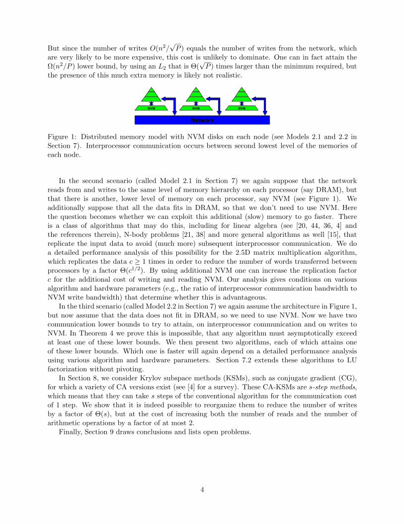
Figure 1: Distributed memory model with NVM disks on each node (see Models 2.1 and 2.2 inSection 7). Interprocessor communication occurs between second lowest level of the memories ofeach node.

In the second scenario (called Model 2.1 in Section 7) we again suppose that the networkreads from and writes to the same level of memory hierarchy on each processor (say DRAM), butthat there is another, lower level of memory on each processor, say NVM (see Figure 1). Weadditionally suppose that all the data fits in DRAM, so that we don’t need to use NVM. Herethe question becomes whether we can exploit this additional (slow) memory to go faster. Thereis a class of algorithms that may do this, including for linear algebra (see [20, 44, 36, 4] andthe references therein), N-body problems [21, 38] and more general algorithms as well [15], thatreplicate the input data to avoid (much more) subsequent interprocessor communication. We doa detailed performance analysis of this possibility for the 2.5D matrix multiplication algorithm,which replicates the data c ≥ 1 times in order to reduce the number of words transferred betweenprocessors by a factor Θ(c1/2). By using additional NVM one can increase the replication factorc for the additional cost of writing and reading NVM. Our analysis gives conditions on variousalgorithm and hardware parameters (e.g., the ratio of interprocessor communication bandwidth toNVM write bandwidth) that determine whether this is advantageous.

In the third scenario (called Model 2.2 in Section 7) we again assume the architecture in Figure 1,but now assume that the data does not fit in DRAM, so we need to use NVM. Now we have twocommunication lower bounds to try to attain, on interprocessor communication and on writes toNVM. In Theorem 4 we prove this is impossible, that any algorithm must asymptotically exceedat least one of these lower bounds. We then present two algorithms, each of which attains oneof these lower bounds. Which one is faster will again depend on a detailed performance analysisusing various algorithm and hardware parameters. Section 7.2 extends these algorithms to LUfactorization without pivoting.

In Section 8, we consider Krylov subspace methods (KSMs), such as conjugate gradient (CG),for which a variety of CA versions exist (see [4] for a survey). These CA-KSMs are s-step methods,which means that they can take s steps of the conventional algorithm for the communication costof 1 step. We show that it is indeed possible to reorganize them to reduce the number of writesby a factor of Θ(s), but at the cost of increasing both the number of reads and the number ofarithmetic operations by a factor of at most 2.

Finally, Section 9 draws conclusions and lists open problems.

4

2 Memory Model and Lower Bounds

Here we both recall an earlier complexity model, which counted the total number of words movedbetween memory units by load and store operations, and present our new model which insteadcounts reads and writes separately. This will in turn require a more detailed execution model,which maps the presence of a particular word of data in memory to a sequence of load/store andthen read/write operations.

The previous complexity model [7] assumed there were two levels of memory, fast and slow.Each memory operation either moved a block of (consecutive) words of data from slow to fastmemory (a “load” operation), or from fast to slow memory (a “store” operation). It counted thetotal number W of words moved in either direction by all memory operations, as well as the totalnumber S of memory operations. The cost model for all these operations was βW + αS, whereβ was the reciprocal bandwidth (seconds per word moved), and α was the latency (seconds permemory operation).

Consider a model memory hierarchy with levels L1, L2, L3, and DRAM, where we assume datadoes not bypass any level: e.g., for data to move from L1 to DRAM it must first move to L2 andthen to L3 before on to DRAM.

Fact 1 For lower bound purposes, we can treat some upper levels, say L1 and L2, as fast memory,and the remaining lower levels, L3 and DRAM, as slow memory. Thus we can model the datamovement between any two consecutive levels of the memory hierarchy.

This technique is well known (cf. [7]), and extends to translating write lower bounds from the two-level model to the memory hierarchy model. Note that converting a WA algorithm for the two-levelmodel into one for the memory hierarchy model is not as straightforward. A similar, more subtleargument can be used to derive lower bounds for the distributed model, by observing the operationof one processor.

Much previous work on communication lower bounds and optimal algorithms explicitly or im-plicitly used these models. Since our goal is to bound the number of writes to a particular memorylevel, we refine this model as follows:

• A load operation, which moves data from slow to fast memory, consists of a read from slowmemory and a write to fast memory.

• A store operation, which moves data from fast to slow memory, consists of a read from fastmemory and a write to slow memory.

• An arithmetic operation can only cause reads and writes in fast memory.

We do not assume a minimum number of reads or writes per arithmetic operation. For example,in the scenario above with fast = L1, L2 and slow = L3,DRAM memories, arbitrarily manyarithmetic operations can be performed on data moved from L2 to L1 without any additional L2

traffic.If we only have a lower bound on the total number of loads and stores, then we don’t know

enough to separately bound the number of writes to either fast or slow memory. And knowinghow many arithmetic operations we perform also does not give us a lower bound on writes to fastmemory. We need the following more detailed model of the entire duration with which a word inmemory is associated with a particular “variable” of the computation. Of course a compiler mayintroduce various temporary variables that are not visible at the algorithmic or source code level.Ignoring these, and considering only, for example, the entries of matrices in matrix multiplication

5

C = A·B, will still let us translate known lower bounds on loads and stores for matrix multiplicationto a lower bound on writes. But when analyzing a particular algorithm, we can take temporaryvariables into account, typically by assuming that variables like loop indices can reside in a higherlevel of the memory hierarchy, and not cause data movement between the levels we are interestedin.

We consider a variable resident in fast memory from the time it first appears to the time it islast used (read or written). It may be updated (written) multiple times during this time period,but it must be associated with a unique data item in the program, for instance a member of a datastructure, like the matrix entry A(i, j) in matrix multiplication. If it is a temporary accumulator,say first for C(1, 1), then for C(1, 2), then between each read/write we can still identify it with aunique entry of C. During the period of time in which a variable is resident, it is stored in a fixedfast memory location and identified with a unique data item in the program. We distinguish twoways a variable’s residency can begin and can end. Borrowing notation from [7], a residency canbegin when

R1: the location is loaded (read from slow memory and written to fast memory), or

R2: the location is computed and written to fast memory, without accessing slow memory; forexample, an accumulator may be initialized to zero just by writing to fast memory.

At the end of residency, we determine another label as follows:

D1: the location is stored (read from fast memory and written to slow memory), or

D2: the location is discarded, i.e., not read or written again while associated with the same variable.

This lets us classify all residencies into one of 4 categories:

R1/D1: The location is initially loaded (read from slow and written to fast memory), and even-tually stored (read from fast and written to slow).

R1/D2: The location is initially loaded (read from slow and written to fast memory), and even-tually discarded.

R2/D1: The location is written to fast memory, and eventually stored (read from fast and writtento slow memory).

R2/D2: The location is written to fast memory, and eventually discarded, without accessing slowmemory.

In each category there is a write to fast memory, and possibly more, if the value in fast memoryis updated. In particular, given all the loads and stores executed by a program, we can uniquelylabel them by the residencies they correspond to. Since each residency results in at least one writeto fast memory, the number of writes to fast memory is at least half the total number of loads andstores (this lower bound corresponds to all residencies being R1/D1). This proves the followingresult:

Theorem 1 Given the preceding memory model, the number of writes to fast memory is at leasthalf the total number of loads and stores between fast and slow memory.

Thus, the various existing communication lower bounds, which are lower bounds on the totalnumber of loads and stores, immediately yield lower bounds on writes to fast memory. In contrast,if most of the residencies are R1/D2 or R2/D2, then we see that no corresponding lower bound on

6

writes to slow memory exists. In this case, if we additionally assume the final output must residein slow memory at the end of execution, we can lower bound the number of writes to slow memoryby the size of the output. For the rest of this paper, we will make this assumption, i.e., that theoutput must be written to slow memory at the end of the algorithm.

2.1 Bounds for 3 or more levels of memory

To be more specific, we consider communication lower bounds on the number W of loads and storesbetween fast and slow memory of the form W = Ω(#flops/f(M)), where #flops is the number ofarithmetic operations performed, M is the size of the fast memory, and f is an increasing function.For example, f(M) = M1/2 for classical linear algebra [7], f(M) = M log2 7−1 for Strassen’s fastmatrix multiplication [8], f(M) = M for the direct N-body problem [15, 21], f(M) = logM forthe FFT [2, 28], and more generally f(M) = M e for some e > 0 for a large class of algorithmsthat access arrays with subscripts that are linear functions of the loop indices [15]. Thus, the lowerbound is a decreasing function of fast memory size M .2.

Corollary 1 Consider a three level memory hierarchy with levels L3, L2, and L1 of sizes M3 >M2 > M1. Let Wij be the number of words moved between Li and Lj. Suppose that W23 =Ω(#flops/f(M2)) and W12 = Ω(#flops/f(M1)). Then the number of writes to L2 is at leastW23/2 = Ω(#flops/f(M2)).

Proof: By Theorem 1 and Fact 1. Note that in Corollary 1 the write lower bound is the smaller of the two communication lower

bounds. This will give us opportunities to do asymptotically fewer writes than reads to all inter-mediate levels of the memory hierarchy.

To formalize the definition of WA for multiple levels of memory hierarchy, we let Lr, Lr−1, . . . , L1

be the levels of memory, with sizes Mr > Mr−1 > · · · > M1. We assume all data fit in the largestlevel Lr. The lower bound on the total number of loads and stores between levels Ls+1 and Ls isΩ(#flops/f(Ms)), which by Theorem 1 is also a lower bound on the number of writes to Ls, whichis “fast memory” with respect to Ls+1. The lower bound on the total number of loads and storesbetween levels Ls and Ls−1 is Ω(#flops/f(Ms−1)), but we know that this does not provide a lowerbound on writes to Ls, which is “slow memory” with respect to Ls−1.

Thus a WA algorithm must perform Θ(#flops/f(Ms)) writes to Ls for s < r, but onlyΘ(output size) writes to Lr.

This is enough for a bandwidth lower bound, but not a latency lower bound, because the latterdepends on the size of the largest message, i.e., the number of messages is bounded below by thenumber of words moved divided by the largest message size. If Ls is being written by data fromLs+1, which is larger, then messages are limited in size by at most Ms, i.e., a message from Ls+1

to Ls cannot be larger than all of Ls. But if Ls is being written from Ls−1, which is smaller, themessages are limited in size by the size Ms−1 of Ls−1. In the examples below, we will see thatthe number of writes to Ls from Ls−1 and Ls+1 (for r > s > 1) are within constant factors of oneanother, so the lower bound on messages written to Ls from Ls+1 will be Θ(#flops/(f(Ms)Ms)),but the lower bound on messages written to Ls from Ls−1 will be Θ(#flops/(f(Ms)Ms−1)), i.e.,larger. We will use this latency analysis for the parallel WA algorithms in Section 7.

We note that the above analysis assumes that the data is so large that it only fits in thelowest, largest level of the memory hierarchy, Lr. When the data is smaller, asymptotic savings

2For some algorithms f may vary across memory levels, e.g., when switching between classical and Strassen-likealgorithms according to matrix size.

7

are naturally possible. For example if all the input and output data fits in some level Ls for s < r,then one can read all the input data from Lr to Ls and then write the output to Ls with no writesto Lt for all t > s. We will refer to this possibility again when we discuss parallel WA algorithmsin Section 7, where Lr’s role is played by the memories of remote processors connected over anetwork.

2.2 Write-buffers

We should mention how to account for write-buffers (a.k.a. burst buffers) [26] in our model. A write-buffer is an extra layer of memory hierarchy in which items that have been written are temporarilystored after a write operation and eviction from cache, and from which they are eventually writtento their final destination (typically DRAM). The purpose is to allow (faster) reads to continueand use the evicted location, and in distributed machines, to accommodate incoming and outgoingdata that arrive faster than the network bandwidth or memory injection rate allow. In the bestcase, this could allow perfect overlap between all reads and writes, and so could decrease the totalcommunication time by a factor of 2 for the sequential model. For the purpose of deriving lowerbounds, we could also model it by treating a cache and its write-buffer as a single larger cache.Either way, this does not change any of our asymptotic analysis, or the need to do many fewerwrites than reads if they are significantly slower than reads (also note that a write-buffer does notavoid the per-word energy cost of writing data).

3 Bounded Data Reuse Precludes Write-Avoiding

In this section we show that if each argument (input data or computed value) of a given computationis used only a constant number of times, then it cannot have a WA algorithm. Let us state thisin terms of the algorithm’s computation directed acyclic graph (CDAG). Recall that for a givenalgorithm and input to that algorithm, its CDAG has a vertex for each input, intermediate andoutput argument, and edges according to direct dependencies. For example, the operation x = y+zinvolves three vertices for x, y, and z, and directed edges (y, x) and (z, x). If two or more binaryoperations both update x, say x = y+z, x = x+w, then this is represented by 5 vertices w, x1, x2, y, zand four edges (y, x1), (z, x1), (x1, x2), (w, x2). Note that an input vertex has no ingoing edges, butan output vertex may have outgoing edges.

Theorem 2 (Bounded reuse precludes WA) Let G be the CDAG of an algorithm A executedon input I on a sequential machine with a two-level memory hierarchy. Let G′ be a subgraph of G.If all vertices of G′, excluding the input vertices, have out-degree at most d, then

1. If the part of the execution corresponding to G′ performs t loads, out of which N are loads ofinput arguments, then the algorithm must do at least d(t−N)/de writes to slow memory.

2. If the part of the execution corresponding to G′ performs a total of W loads and stores, ofwhich at most half are loads of input arguments, then the algorithm must do Ω(W/d) writesto slow memory.

Proof: Of the t loads from slow memory, t−N must be loads of intermediate results rather thaninputs. These had to be previously written to slow memory. Since the maximum out-degree ofany intermediate data vertex is d, at least d(t−N)/de distinct intermediate arguments have beenwritten to slow memory. This proves (1).

8

If the execution corresponding to G′ does at least W/10d writes to the slow memory, then we aredone. Otherwise, there are at least t = 10d−1

10d W loads. Applying (1) with N ≤ W/2, we conclude

that the number of writes to slow memory is at least d(10d−110d −12)W/de = Ω(W/d), proving (2).

We next demonstrate the use of Theorem 2, applying it to Cooley-Tukey FFT and Strassen’s(and “Strassen-like”) matrix multiplication, thus showing they do not admit WA algorithms.

Corollary 2 (WA FFT is impossible) Consider executing the Cooley-Tukey FFT on a vectorof size n on a sequential machine with a two-level memory hierarchy whose fast memory has sizeM n. Then the number of stores is asymptotically the same as the total number of loads andstores, namely Ω(n log n/ logM).

Proof: The Cooley-Tukey FFT has out-degree bounded by d = 2, input vertices included. By[28], the total number of loads and stores to slow memory performed by any implementation ofthe Cooley-Tukey FFT algorithm on an input of size n is W = Ω(n log n/ logM). Since W isasymptotically larger than n, and so also larger than N = 2n = the number of input loads, theresult follows by applying Theorem 2 with G′ = G.

Corollary 3 (WA Strassen is impossible) Consider executing Strassen’s matrix multiplicationon n-by-n matrices on a sequential machine with a two-level memory hierarchy whose fast memoryhas size M n. Then the number of stores is asymptotically the same as the total number of loadsand stores, namely Ω(nω0/Mω0/2−1), where ω0 = log2 7.

Proof: We consider G′ to be the induced subgraph of the CDAG that includes the vertices ofthe scalar multiplications and all their descendants, including the output vertices. As described in[8] (G′ is denoted there by DecC), G′ is connected, includes no input vertices (N = 0), and themaximum out-degree of any vertex in G′ is d = 4. The lower bound from [8] on loads and stores forG′, and so also for the entire algorithm, is W = Ω(nω0/Mω0/2−1). Plugging these into Theorem 2the corollary follows.

Corollary 3 extends to any Strassen-like algorithm (defined in [8]), with ω0 replaced with thecorresponding algorithm’s exponent. Note that trying to apply the above to classical matrix multi-plication does not work: G′ is a disconnected graph, hence not satisfying the requirement in [8] forbeing Strassen-like. Indeed, WA algorithms for classical matrix multiplication do exist, as we latershow. However, Corollary 3 does extend to Strassen-like rectangular matrix multiplication: theydo not admit WA algorithms (see [5] for corresponding communication cost lower bounds that takeinto account the three possibly distinct matrix dimensions). And while G′ may be disconnectedfor some Strassen-like rectangular matrix multiplications, this is taken into account in the lowerbounds of [5].

4 Examples of WA Algorithms

In this section we give sequential WA algorithms for classical matrix multiplication C = AB,solving systems of linear equations TX = B where T is triangular and B has multiple columns bysuccessive substitution (TRSM), Cholesky factorization A = LLT , and the direct N-body problemwith multiple particle interactions. In all cases we give an explicit solution for a two-level memoryhierarchy, and explain how to extend to multiple levels.

In all cases the WA algorithms are blocked explicitly using the fast memory size M . In fact theyare known examples of CA algorithms, but we will see that not all explicitly blocked CA algorithmsare WA: the nesting order of the loops must be chosen appropriately.

9

We also assume that the programmer has explicit control over all data motion, and so statethis explicitly in the algorithms. Later in Section 6 we present measurements about how close tothe minimum number of writes machines with hardware cache policies can get.

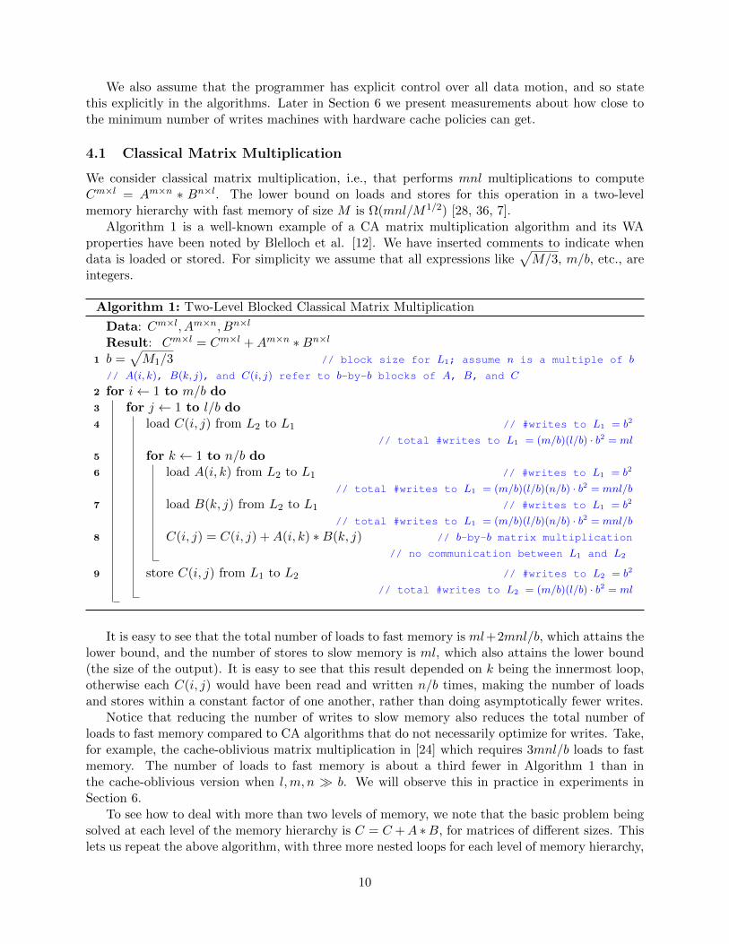
4.1 Classical Matrix Multiplication

We consider classical matrix multiplication, i.e., that performs mnl multiplications to computeCm×l = Am×n ∗ Bn×l. The lower bound on loads and stores for this operation in a two-levelmemory hierarchy with fast memory of size M is Ω(mnl/M1/2) [28, 36, 7].

Algorithm 1 is a well-known example of a CA matrix multiplication algorithm and its WAproperties have been noted by Blelloch et al. [12]. We have inserted comments to indicate whendata is loaded or stored. For simplicity we assume that all expressions like

√M/3, m/b, etc., are

integers.

Algorithm 1: Two-Level Blocked Classical Matrix Multiplication

Data: Cm×l, Am×n, Bn×l

Result: Cm×l = Cm×l +Am×n ∗Bn×l

1 b =√M1/3 // block size for L1; assume n is a multiple of b

// A(i, k), B(k, j), and C(i, j) refer to b-by-b blocks of A, B, and C

2 for i← 1 to m/b do3 for j ← 1 to l/b do4 load C(i, j) from L2 to L1 // #writes to L1 = b2

// total #writes to L1 = (m/b)(l/b) · b2 = ml

5 for k ← 1 to n/b do6 load A(i, k) from L2 to L1 // #writes to L1 = b2

// total #writes to L1 = (m/b)(l/b)(n/b) · b2 = mnl/b

7 load B(k, j) from L2 to L1 // #writes to L1 = b2

// total #writes to L1 = (m/b)(l/b)(n/b) · b2 = mnl/b

8 C(i, j) = C(i, j) +A(i, k) ∗B(k, j) // b-by-b matrix multiplication

// no communication between L1 and L2

9 store C(i, j) from L1 to L2 // #writes to L2 = b2

// total #writes to L2 = (m/b)(l/b) · b2 = ml

It is easy to see that the total number of loads to fast memory is ml+2mnl/b, which attains thelower bound, and the number of stores to slow memory is ml, which also attains the lower bound(the size of the output). It is easy to see that this result depended on k being the innermost loop,otherwise each C(i, j) would have been read and written n/b times, making the number of loadsand stores within a constant factor of one another, rather than doing asymptotically fewer writes.

Notice that reducing the number of writes to slow memory also reduces the total number ofloads to fast memory compared to CA algorithms that do not necessarily optimize for writes. Take,for example, the cache-oblivious matrix multiplication in [24] which requires 3mnl/b loads to fastmemory. The number of loads to fast memory is about a third fewer in Algorithm 1 than inthe cache-oblivious version when l,m, n b. We will observe this in practice in experiments inSection 6.

To see how to deal with more than two levels of memory, we note that the basic problem beingsolved at each level of the memory hierarchy is C = C +A ∗B, for matrices of different sizes. Thislets us repeat the above algorithm, with three more nested loops for each level of memory hierarchy,

10

in the same order as above. More formally, we use induction: Suppose we have a WA algorithm forr memory levels Lr, . . . , L1, and we add one more smaller one L0 with memory size M0. We needto show that adding three more innermost nested loops will

(1) not change the number of writes to Lr, . . . , L2,

(2) increase the number of writes to L1, O(mnl/√M1), by at most a constant factor, and

(3) do O(mnl/M1/20 ) writes to L0.

(1) and (3) follow immediately by the structure of the algorithm. To prove (2), we note that L1

gets mnl/(M1/3)3/2 blocks of A, B, and C, each square of dimension b1 = (M1/3)1/2, to multiplyand add. For each such b1-by-b1 matrix multiplication, it will partition the matrices into blocks ofdimension b0 = (M0/3)1/2 and multiply them using Algorithm 1, resulting in a total of b21 writes toL1 from L0. Since this happens mnl/(M1/3)3/2 times, the total number of writes to L1 from L0 ismnl/(M1/3)3/2 · b21 = mnl/(M1/3)1/2 as desired.

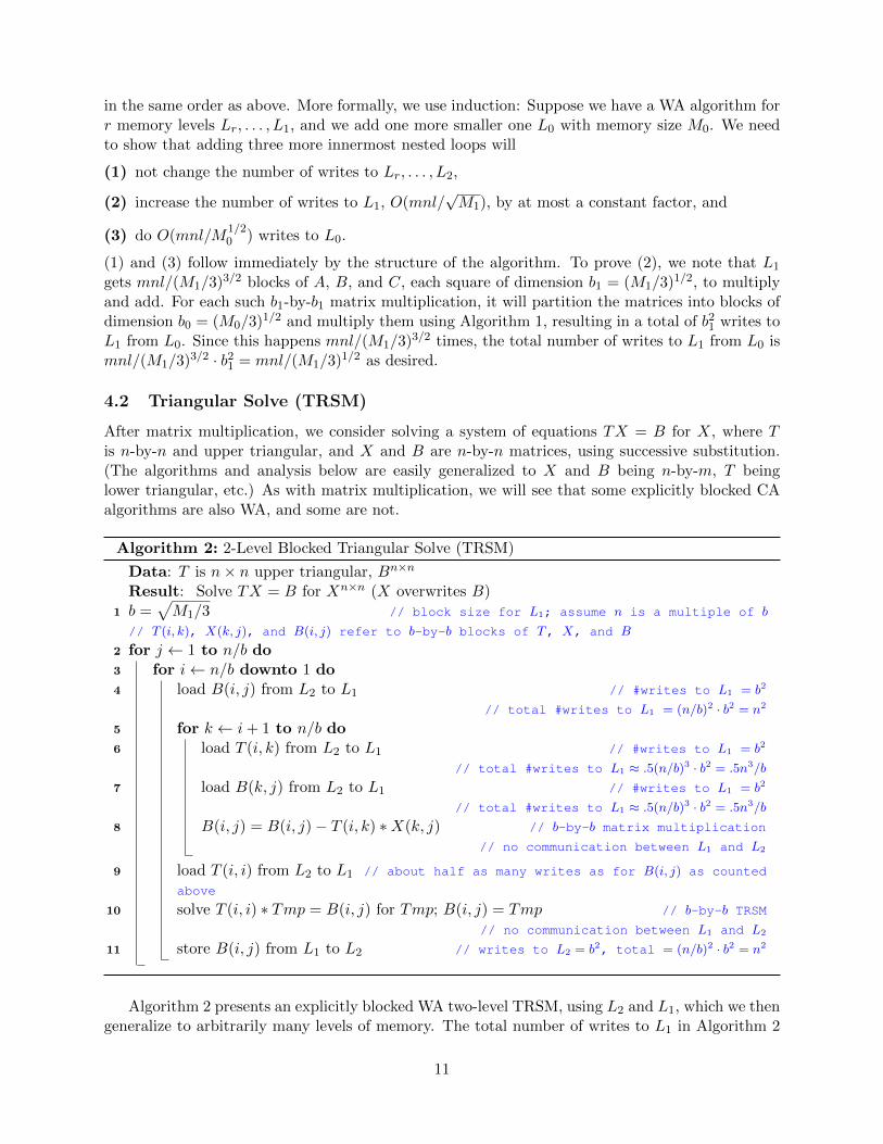
4.2 Triangular Solve (TRSM)

After matrix multiplication, we consider solving a system of equations TX = B for X, where Tis n-by-n and upper triangular, and X and B are n-by-n matrices, using successive substitution.(The algorithms and analysis below are easily generalized to X and B being n-by-m, T beinglower triangular, etc.) As with matrix multiplication, we will see that some explicitly blocked CAalgorithms are also WA, and some are not.

Algorithm 2: 2-Level Blocked Triangular Solve (TRSM)

Data: T is n× n upper triangular, Bn×n

Result: Solve TX = B for Xn×n (X overwrites B)1 b =

√M1/3 // block size for L1; assume n is a multiple of b

// T (i, k), X(k, j), and B(i, j) refer to b-by-b blocks of T, X, and B

2 for j ← 1 to n/b do3 for i← n/b downto 1 do4 load B(i, j) from L2 to L1 // #writes to L1 = b2

// total #writes to L1 = (n/b)2 · b2 = n2

5 for k ← i+ 1 to n/b do6 load T (i, k) from L2 to L1 // #writes to L1 = b2

// total #writes to L1 ≈ .5(n/b)3 · b2 = .5n3/b

7 load B(k, j) from L2 to L1 // #writes to L1 = b2

// total #writes to L1 ≈ .5(n/b)3 · b2 = .5n3/b

8 B(i, j) = B(i, j)− T (i, k) ∗X(k, j) // b-by-b matrix multiplication


9 load T (i, i) from L2 to L1 // about half as many writes as for B(i, j) as counted

above

10 solve T (i, i) ∗ Tmp = B(i, j) for Tmp; B(i, j) = Tmp // b-by-b TRSM


11 store B(i, j) from L1 to L2 // writes to L2 = b2, total = (n/b)2 · b2 = n2

Algorithm 2 presents an explicitly blocked WA two-level TRSM, using L2 and L1, which we thengeneralize to arbitrarily many levels of memory. The total number of writes to L1 in Algorithm 2

11

is seen to be n3/b + 3n2/2, and the number of writes to L2 is just n2, the size of the output.So Algorithm 2 is WA for L2. Again there is a (correct) CA version of this algorithm for anypermutation of the three loops on i, j, and k, but the algorithm is only WA if k is the innermostloop, so that B(i, j) may be updated many times without writing intermediate values to L2. Thisis analogous to the analysis of Algorithm 1.

Now we generalize Algorithm 2 to multiple levels of memory. Analogously to Algorithm 1,Algorithm 2 calls itself on smaller problems at each level of the memory hierarchy, but also callsAlgorithm 1. We again use induction, assuming the algorithm is WA with memory levels Lr, . . . , L1,and add one more smaller level L0 of size M0. We then replace line 8, B(i, j) = B(i, j)− T (i, k) ∗X(k, j), by a call to Algorithm 1 but use a block size of b0 = (M0/3)1/2, and replace line 10, thatsolves T (i, i) ∗ Tmp = B(i, j), with a call to Algorithm 2, again with block size b0.

As with matrix multiplication, there are three things to prove in the induction step to showthat this is WA. As before (1) follows since adding a level of memory does not change the numberof writes to Lr, . . . , L2. Let b1 = (M1/3)1/2. To prove (2), we note that by induction, O(n3/

√M1)

words are written to L1 from L2 in the form of b1-by-b1 matrices which are inputs to either matrixmultiplication or TRSM. Thus the size of the outputs of each of these matrix multiplications orTRSMs is also b1-by-b1, and so also consists of a total of O(n3/

√M1) words. Since both matrix

multiplication and TRSM only write the output once to L1 from L0 for each matrix multiplicationor TRSM, the total number of additional writes to L1 from L0 is O(n3/

√M1), the same as the

number of writes to L1 from L2, as desired. (3) follows by a similar argument.

4.3 Cholesky Factorization

Cholesky factorizes a real symmetric positive-definite matrix A into the product A = LLT of alower triangular matrix L and its transpose LT , and uses both matrix multiplication and TRSMas building blocks. We will once again see that some explicitly blocked CA algorithms are also WA(left-looking Cholesky), and some are not (right-looking). Based on the similar structure of otherone-sided factorizations in linear algebra, we conjecture that similar conclusions hold for LU, QR,and related factorizations.

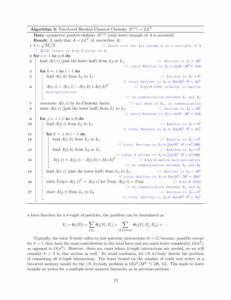
Algorithm 3 presents an explicitly blocked WA left-looking two-level Cholesky, using L2 and L1,which we will again use to describe how to write a version for arbitrarily many levels of memory.

As can be seen in Algorithm 3, the total number of writes to L2 is about n2/2, because theoutput (lower half of A) is stored just once, and the number of writes to L1 is Θ(n3/

√M1).

By using WA versions of the b-by-b matrix multiplications, TRSMs, and Cholesky factorizations,this WA property can again be extended to multiple levels of memory, using an analogous inductionargument.

This version of Cholesky is called left-looking because the innermost (k) loop starts from theoriginal entries of A(j, i) in block column i, and completely computes the corresponding entries ofL by reading entries A(i, k) and A(j, k) to its left. In contrast, a right-looking algorithm woulduse block column i to immediately update all entries of A to its right, i.e., the Schur complement,leading to asymptotically more writes.

4.4 Direct N-Body

Consider a system of particles (bodies) where each particle exerts physical forces on every otherparticle and moves according to the total force on it. The direct N-body problem simulates thisby calculating all forces from all k-tuples of particles directly (k = 1, 2, . . .). Letting P be an inputarray of N particles, F be an output array of accumulated forces on each particle in P , and Φk be

12

Algorithm 3: Two-Level Blocked Classical Cholesky An×n = LLT

Data: symmetric positive-definite An×n (only lower triangle of A is accessed)Result: L such that A = LLT (L overwrites A)

1 b =√M1/3 // block size for L1; assume n is a multiple of b

// A(i, k) refers to b-by-b block of A

2 for i← 1 to n/b do3 load A(i, i) (just the lower half) from L2 to L1 // #writes to L1 = .5b2

// total #writes to L1 = (n/b) · .5b2 = .5nb

4 for k ← 1 to i− 1 do5 load A(i, k) from L2 to L1 // #writes to L1 = b2

// total #writes to L1 ≈ .5(n/b)2 · b2 = .5n2

6 A(i, i) = A(i, i)−A(i, k) ∗A(i, k)T // b-by-b SYRK (similar to matrix

multiplication)


7 overwrite A(i, i) by its Cholesky factor // all done in L1, no communication

8 store A(i, i) (just the lower half) from L1 to L2 // #writes to L2 = .5b2

// total #writes to L2 = (n/b) · .5b2 = .5nb

9 for j ← i+ 1 to n/b do10 load A(j, i) from L2 to L1 // #writes to L1 = b2


11 for k = 1 to i− 1 do12 load A(i, k) from L2 to L1 // #writes to L1 = b2

// total #writes to L1 ≈ 16(n/b)3 · b2 = n3/(6b)

13 load A(j, k) from L2 to L1 // #writes to L1 = b2

// total # writes to L1 ≈ 16(n/b)3 · b2 = n3/(6b)

14 A(j, i) = A(j, i)−A(j, k) ∗A(i, k)T // b-by-b matrix multiplication


15 load A(i, i) (just the lower half) from L2 to L1 // #writes to L1 = .5b2

// total #writes to L1 ≈ .5(n/b)2 · .5b2 = .25n2

16 solve Tmp ∗A(i, i)T = A(j, i) for Tmp; A(j, i) = Tmp // b-by-b TRSM


17 store A(j, i) from L1 to L2 // #writes to L2 = b2


a force function for a k-tuple of particles, the problem can be formulated as

Fi = Φ1(Pi) +∑i 6=j

Φ2(Pi, Pj) +∑

i 6=j 6=m6=iΦ3(Pi, Pj , Pm) + · · ·

Typically, the term N-body refers to just pairwise interactions (k = 2) because, possibly exceptfor k = 1, they have the most contribution to the total force and are much lower complexity, O(n2),as opposed to O(nk). However, there are cases where k-tuple interactions are needed, so we willconsider k > 2 in this section as well. To avoid confusion, let (N, k)-body denote the problemof computing all k-tuple interactions. The lower bound on the number of reads and writes in atwo-level memory model for the (N, k)-body problem is O(nk/Mk−1) [38, 15]. This leads to lowerbounds on writes for a multiple-level memory hierarchy as in previous sections.

13

Throughout this section, we will use the particle size as a unit for memory, i.e., L1 and L2 canstore M1 and M2 particles, respectively. We assume that a force is of the same size as a particle.

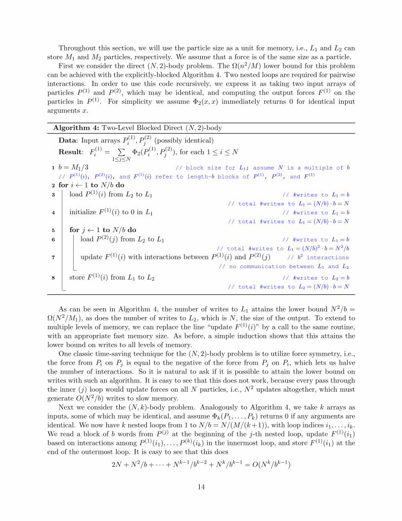
First we consider the direct (N, 2)-body problem. The Ω(n2/M) lower bound for this problemcan be achieved with the explicitly-blocked Algorithm 4. Two nested loops are required for pairwiseinteractions. In order to use this code recursively, we express it as taking two input arrays ofparticles P (1) and P (2), which may be identical, and computing the output forces F (1) on theparticles in P (1). For simplicity we assume Φ2(x, x) immediately returns 0 for identical inputarguments x.

Algorithm 4: Two-Level Blocked Direct (N, 2)-body

Data: Input arrays P(1)i , P

(2)j (possibly identical)

Result: F(1)i =

∑1≤j≤N

Φ2(P(1)i , P

(2)j ), for each 1 ≤ i ≤ N

1 b = M1/3 // block size for L1; assume N is a multiple of b

// P (1)(i), P (2)(i), and F (1)(i) refer to length-b blocks of P (1), P (2), and F (1)

2 for i← 1 to N/b do

3 load P (1)(i) from L2 to L1 // #writes to L1 = b

// total #writes to L1 = (N/b) · b = N

4 initialize F (1)(i) to 0 in L1 // #writes to L1 = b


5 for j ← 1 to N/b do

6 load P (2)(j) from L2 to L1 // #writes to L1 = b

// total #writes to L1 = (N/b)2 · b = N2/b

7 update F (1)(i) with interactions between P (1)(i) and P (2)(j) // b2 interactions


8 store F (1)(i) from L1 to L2 // #writes to L2 = b


As can be seen in Algorithm 4, the number of writes to L1 attains the lower bound N2/b =Ω(N2/M1), as does the number of writes to L2, which is N , the size of the output. To extend tomultiple levels of memory, we can replace the line “update F (1)(i)” by a call to the same routine,with an appropriate fast memory size. As before, a simple induction shows that this attains thelower bound on writes to all levels of memory.

One classic time-saving technique for the (N, 2)-body problem is to utilize force symmetry, i.e.,the force from Pi on Pj is equal to the negative of the force from Pj on Pi, which lets us halvethe number of interactions. So it is natural to ask if it is possible to attain the lower bound onwrites with such an algorithm. It is easy to see that this does not work, because every pass throughthe inner (j) loop would update forces on all N particles, i.e., N2 updates altogether, which mustgenerate O(N2/b) writes to slow memory.

Next we consider the (N, k)-body problem. Analogously to Algorithm 4, we take k arrays asinputs, some of which may be identical, and assume Φk(P1, . . . , Pk) returns 0 if any arguments areidentical. We now have k nested loops from 1 to N/b = N/(M/(k+1)), with loop indices i1, . . . , ik.We read a block of b words from P (j) at the beginning of the j-th nested loop, update F (1)(i1)based on interactions among P (1)(i1), . . . , P

(k)(ik) in the innermost loop, and store F (1)(i1) at theend of the outermost loop. It is easy to see that this does

2N +N2/b+ · · ·+Nk−1/bk−2 +Nk/bk−1 = O(Nk/bk−1)

14

writes to L1, and N writes to L2, attaining the lower bounds on writes. Again, calling itselfrecursively extends its WA property to multiple levels of memory. Now there is a penalty of afactor of k!, in both arithmetic and number of reads, which can be quite large, for not takingadvantage of symmetry in the arguments of Φk in order to minimize writes.

5 Cache-Oblivious Algorithms Cannot be Write-Avoiding

Following [23] and [11, Section 4], we define a cache-oblivious (CO) algorithm as one in whichthe sequence of instructions executed does not depend on the memory hierarchy of the machine;otherwise it is called cache-aware. Here we prove that sequential CO algorithms cannot be WA.This is in contrast to the existence of many CO algorithms that are CA.

As stated, our proof applies to any algorithm to which the lower bounds analysis of [7] applies,so most direct linear algebra algorithms like classical matrix multiplication, other BLAS routines,Cholesky, LU decomposition, etc., for sparse as well as dense matrices, and related algorithms liketensor contractions and Floyd-Warshall all-pairs shortest-paths in a graph. (At the end of thesection we suggest extensions to other algorithms.)

For this class of algorithms, given a set S of triples of nonnegative integers (i, j, k), for alltriples in S the algorithm reads two array locations A(i, k) and B(k, j) and updates array locationC(i, j); for simplicity we call this update operation an “inner loop iteration”. This obviouslyincludes dense matrix multiplication, for which S = (i, j, k) : 1 ≤ i, j, k ≤ n and C(i, j) =C(i, j) +A(i, k) ∗B(k, j), but also other algorithms like LU because the matrices A, B, and C mayoverlap or be identical.

A main tool we need to use is the Loomis-Whitney inequality [40]. Given a fixed number ofdifferent entries of A, B, and C that are available (say because they are in fast memory), theLoomis-Whitney inequality bounds the number of inner loop iterations that may be performed:#iterations ≤

√|A| · |B| · |C|, where |A| is the number of available entries of A, etc.

Following the argument in [7], and introduced in [36], we consider a program to be a sequenceof load (read from slow, write to fast memory), store (read from fast, write to slow memory), andarithmetic/logical instructions. Then assuming fast memory is of size M , we analyze the algorithmas follows:

1. Break the stream of instructions into segments, where each segment contains exactly M loadand store instructions, as well as the intervening arithmetic/logical instructions. Assumingthere are no R2/D2 residencies (see Section 2) then this means that the number of distinctentries available during the segment to perform arithmetic/logical instructions is at most 4M(see [7] for further explanation of where the bound 4M arises; this includes all the linearalgebra and related algorithms mentioned above). We will also assume that no entries of Care discarded, i.e., none are D2.

2. Using Loomis-Whitney and the bound 4M on the number of entries of A, B, and C, webound the maximum number of inner loop iterations that can be performed during a segmentby√

(4M)3 = 8M3/2.

3. Denoting the total number of inner loop iterations by |S|, we can bound below the numberof complete segments by s = b|S|/(8M3/2)c.

4. Since each complete segment performs M load and store instructions, the total number ofload and store instructions is at least M · s = M · b|S|/(8M3/2)c ≥ |S|/(8M1/2)−M . When|S| M3/2, this is close to |S|/(8M1/2) = Ω(|S|/M1/2). We note that the floor function

15

accommodates the situation where the inputs are all small enough to fit in fast memory atthe beginning of the algorithm, and for the output to be left in fast memory at the end ofthe algorithm, and so no loads or stores are required.

Theorem 3 Consider an algorithm that satisfies the assumptions presented above. First, supposethat for a particular input I, the algorithm executes the same sequence of instructions, independentof the memory hierarchy. Second, suppose that for the same input I and fast memory size M ,the algorithm is CA in the following sense: the total number of loads and stores it performs isbounded above by c · |S|/M1/2 for some constant c ≥ 1/8. (Note that c cannot be less than 1/8 byparagraph 4 above.) Then the algorithm cannot be WA in the following sense: When executed usinga sufficiently smaller fast memory size M ′ < M/(64c2), the number of writes Ws to slow memoryis at least

Ws ≥b|S|/(8M3/2)c

16c− 1·(M

64c2−M ′

)= Ω

(|S|M1/2

). (1)

For example, consider n-by-n dense matrix multiplication, where |S| = n3. A WA algorithm wouldperform O(n2) writes to slow memory, but a CO algorithm would perform at least Ω(n3/M1/2)writes with a smaller cache size M ′.Proof: For a particular input, let s be the number of complete segments in the algorithm. Thenby assumption s ·M ≤ c|S|/M1/2. This means the average number of inner loop iterations persegment, Aavg = |S|/s, is at least Aavg ≥ M3/2/c. By Loomis-Whitney, the maximum number ofinner loop iterations per segment is Amax ≤ 8M3/2. Now write s = s1 + s2 where s1 is the numberof segments containing at least Aavg/2 inner loop iterations, and s2 is the number of segmentscontaining less than Aavg/2 inner loop iterations. Letting ai be the number of inner loop iterationsin segment i, we get

Aavg =s∑i=1

ais

=

∑i:ai<Aavg/2

ai +∑

i:ai≥Aavg/2ai

s≤ s2 ·Aavg/2 + s1 ·Amax

s1 + s2,

or rearranging,

s2 ≤ 2

(AmaxAavg

− 1

)s1 ≤ 2(8c− 1)s1,

so s = s1 + s2 ≤ (16c− 1)s1, and we see that s1 ≥ s/(16c− 1) segments perform at least Aavg/2 ≥M3/2/(2c) inner loop iterations.

Next, since there are at most 4M entries of A and B available during any one of these s1segments, Loomis-Whitney tells us that the number |C| of entries of C written to slow memory

during any one of these segments must satisfy M3/2

2c ≤ (4M · 4M · |C|)1/2 or M64c2≤ |C|.

Now consider running the algorithm with a smaller cache size M ′ < M/(64c2), and considerwhat happens during any one of these s1 segments. Since at least M

64c2different entries of C are

written and none are discarded (D2), at least M64c2−M ′ entries must be written to slow memory

during a segment. Thus the total number Ws of writes to slow memory satisfies

Ws ≥ s1 ·(M

64c2−M ′

)≥ s

16c− 1·(M

64c2−M ′

)≥ b|S|/(8M

3/2)c16c− 1

·(M

64c2−M ′

)= Ω

(|S|M1/2

),

as claimed.

Corollary 4 Suppose a CO algorithm (assuming the same hypotheses as Theorem 3) is CA for allinputs and fast memory sizes M , in the sense that it performs at most c · |S|/M1/2 loads and stores

16

for some constant c ≥ 1/8. Then it cannot be WA in the following sense: for all fast memory sizesM , the algorithm performs

Ws ≥b|S|/(8(128c2M)3/2)c

16c− 1·M = Ω

(|S|M1/2

)writes to slow memory.

Proof: For ease of notation, denote the M in the statement of the Corollary by M . Then applyTheorem 3 with M ′ = M , and M = 128c2M , so that the lower bound in (1) becomes

Ws ≥b|S|/(8(128c2M)3/2)c

16c− 1· M = Ω

(|S|M1/2

).

We note that our proof technique applies more generally to the class of algorithms considered

in [15], i.e., algorithms that can be expressed with a set S of tuples of integers, and where therecan be arbitrarily many arrays with arbitrarily many subscripts in an inner loop iteration, as longas each subscript is an affine function of the integers in the tuple (pointers are also allowed). Theformulation of Theorem 3 will change because the exponents 3/2 and 1/2 will vary depending onthe algorithm, and which arrays are read and written.

6 Write-Avoidance in Practice: Hardware Counter Measurementsand Cache Replacement Policies

The WA properties of the algorithms described in Section 4 depend on explicitly controlling datamovement between caches. However, most instruction sets like x86-64 do not provide the user withan elaborate interface for explicitly managing data movement between caches. Typically, the useris allowed to specify the order of execution of the instructions in the algorithm addressing databy virtual memory address, while the mapping from virtual address to physical location in thecaches is determined by hardware cache management (cache replacement and coherence policy).Therefore, an analysis of the behavior of an algorithm on real caches must account for the interactionbetween the execution order of the instructions and the hardware cache management. Further, thehardware management must be conducive to the properties desired by the user (e.g., minimizingdata movement between caches, or in our case, write-backs to the memory).

In this section, we provide hardware counter measurements of caching events for several in-struction orders in the classical matrix multiplication algorithm to measure this interaction witha view towards understanding the gap between practice and the theory in previous sections. Theinstruction orders we report include the cache-oblivious order from [24] and the WA orders for var-ious cache levels from Section 4 and Intel’s MKL dgemm. Drawing upon this data, we hypothesizeand prove that the Least Recently Used (LRU) replacement policy is good at minimizing writes inthe two-level write-avoiding algorithms in Section 4.

6.1 Hardware Counter Measurements

Machine and experimental setup. We choose for our measurements the Nehalem-EX microar-chitecture based Intel Xeon 7560 processor since its performance counters are well documented (corecounters in [34, Table 19-13] and Xeon 7500-series uncore counters in [31]). We program the hard-ware counters using a customized version of the Intel PCM 2.4 tool [32]. The machine we use has

17

an L1 cache of size 32KB, an L2 cache of size 256KB per physical core, and an L3 cache of size24MB (sum of 8 L3 banks on a die) shared among eight cores. All caches are organized into 64-bytecache lines. We use the hugectl tool [39] for allocating “huge” virtual memory pages to avoidTLB misses. The Linux kernel version is 3.6.1. We use Intel MKL shipped with Composer XE2013 (package 2013.3.163). All the experiments are started from a “cold cache” state, i.e., none ofthe matrix entries are cached. This makes the experiments with smaller instances more predictableand repeatable.

Coherence policy. This architecture uses the MESIF coherence policy [30]. Data read directlyfrom DRAM is cached in the “Exclusive”(E) state. Data that has been modified (written by aprocessor) is cached locally by a processor in a “Modified” (M) state. All our experiments aresingle threaded and thus the “Shared” (S) and “Forward” (F) state are less relevant. When amodified cache line is evicted by the replacement policy, its contents are written back to a lowercache level [33, Section 2.1.4], or in the case of L3 cache on this machine, to DRAM.

Counters. To measure the number of writes to slow memory, we measure the evictions of modifiedcache lines from L3 cache as these are obligatory write-backs to DRAM. We use the C-box eventLLC VICTIMS.M [31] for this. We also measure the number of exclusive lines evicted from L3(which are presumably forgotten) using the event LLC VICTIMS.E. We measure the number ofreads from DRAM into L3 cache necessitated by L3 cache misses with the performance eventLLC S FILLS.E.

Replacement Policy. To the best of our knowledge, Intel does not officially state the cachereplacement policies used in its microarchitectures. However, it has been speculated and informallyacknowledged by Intel [22, 35, 27] that the L3 replacement policy on the Nehalem microarchitectureis the 3-bit LRU-like “clock algorithm” [17]. This algorithm attempts to mimic the LRU policyby maintaining a 3-bit marker to indicate recent usage within an associative set of cache lines. Toevict a cache line, the hardware searches for, within the associative set in clockwise order, a linewhich has not been recently used (marked 000). If such a line is not found, the markers on allcache lines are decremented and the search for a recently unused line is performed again. Cacheline hits increase the marker. It has also been speculated [27] that Intel has adopted a new cachereplacement policy similar to RRIP [37] from the Ivy Bridge microarchitecture onwards.

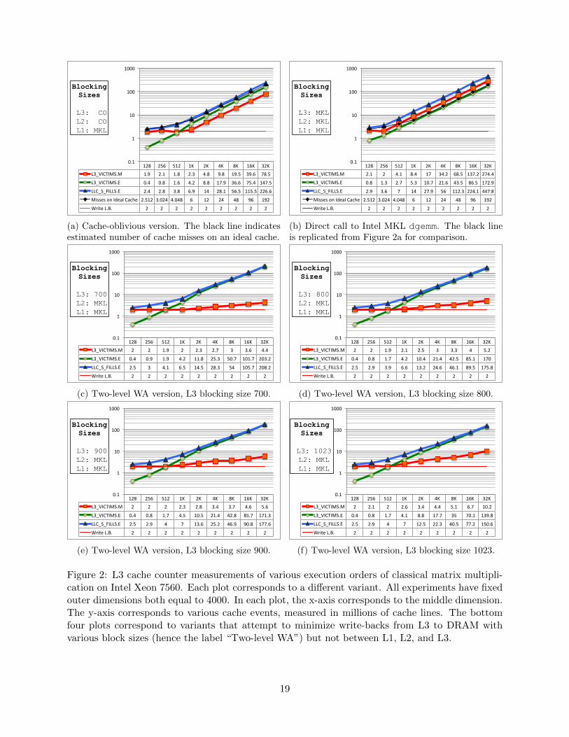
Experimental Data. The experiments in Figure 2 demonstrate the L3 behavior of differentversions of the classical double precision matrix multiplication algorithm that computes C = A∗B.Let the dimensions of A,B and C be l-by-m, m-by-n and l-by-n respectively. Each of the six plotsin Figure 2 correspond to instances of dimensions 4000-by-m-by-4000 where m takes the valuesfrom the set 128, 256, . . . , 32 · 210. In each of these instances, the size of the output array C is aconstant 40002 · 8 B = 122.07 MB which translates to 2.0 million cache lines. This is marked with ahorizontal red line in each plot. The arrays A and B vary in size between the instances. All plotsshow trends in the hardware events LLC VICTIMS.M, LLC VICTIMS.E, and LLC S FILLS.E, andreport measurements in millions of cache lines. In instances where m ≤ 512, arrays A and B fit inthe L3 cache, while in other instances (m ≥ 1024) they overflow L3 cache.

The first version in Figure 2a is a recursive cache-oblivious version [24] that splits the probleminto two along the largest of the three dimensions l, m, and n and recursively computes the twomultiplications in sequence. The base case of the recursion fits in the L1 cache and makes a call to

18

128 256 512 1K 2K 4K 8K 16K 32K L3_VICTIMS.M 1.9 2.1 1.8 2.3 4.8 9.8 19.5 39.6 78.5

L3_VICTIMS.E 0.4 0.8 1.6 4.2 8.8 17.9 36.6 75.4 147.5

LLC_S_FILLS.E 2.4 2.8 3.8 6.9 14 28.1 56.5 115.5 226.6

Misses on Ideal Cache 2.512 3.024 4.048 6 12 24 48 96 192

Write L.B. 2 2 2 2 2 2 2 2 2

0.1

1

10

100

1000

Blocking Sizes

L3: CO L2: CO L1: MKL

(a) Cache-oblivious version. The black line indicatesestimated number of cache misses on an ideal cache.

128 256 512 1K 2K 4K 8K 16K 32K L3_VICTIMS.M 2.1 2 4.1 8.4 17 34.2 68.5 137.2 274.4

L3_VICTIMS.E 0.8 1.3 2.7 5.3 10.7 21.6 43.5 86.5 172.9

LLC_S_FILLS.E 2.9 3.6 7 14 27.9 56 112.3 224.1 447.8

Misses on Ideal Cache 2.512 3.024 4.048 6 12 24 48 96 192

Write L.B. 2 2 2 2 2 2 2 2 2

0.1

1

10

100

1000

Blocking Sizes

L3: MKL L2: MKL L1: MKL

(b) Direct call to Intel MKL dgemm. The black lineis replicated from Figure 2a for comparison.

128 256 512 1K 2K 4K 8K 16K 32K L3_VICTIMS.M 2 2 1.9 2 2.3 2.7 3 3.6 4.4

L3_VICTIMS.E 0.4 0.9 1.9 4.2 11.8 25.3 50.7 101.7 203.2

LLC_S_FILLS.E 2.5 3 4.1 6.5 14.5 28.3 54 105.7 208.2

Write L.B. 2 2 2 2 2 2 2 2 2

0.1

1

10

100

1000

Blocking Sizes

L3: 700 L2: MKL L1: MKL

(c) Two-level WA version, L3 blocking size 700.

128 256 512 1K 2K 4K 8K 16K 32K L3_VICTIMS.M 2 2 1.9 2.1 2.5 3 3.3 4 5.2

L3_VICTIMS.E 0.4 0.8 1.7 4.2 10.4 21.4 42.5 85.1 170

LLC_S_FILLS.E 2.5 2.9 3.9 6.6 13.2 24.6 46.1 89.5 175.8

Write L.B. 2 2 2 2 2 2 2 2 2

0.1

1

10

100

1000

Blocking Sizes

L3: 800 L2: MKL L1: MKL

(d) Two-level WA version, L3 blocking size 800.

128 256 512 1K 2K 4K 8K 16K 32K L3_VICTIMS.M 2 2 2 2.3 2.8 3.4 3.7 4.6 5.6

L3_VICTIMS.E 0.4 0.8 1.7 4.5 10.5 21.4 42.8 85.7 171.3

LLC_S_FILLS.E 2.5 2.9 4 7 13.6 25.2 46.9 90.8 177.6

Write L.B. 2 2 2 2 2 2 2 2 2

0.1

1

10

100

1000

Blocking Sizes

L3: 900 L2: MKL L1: MKL

(e) Two-level WA version, L3 blocking size 900.

128 256 512 1K 2K 4K 8K 16K 32K L3_VICTIMS.M 2 2.1 2 2.6 3.4 4.4 5.1 6.7 10.2

L3_VICTIMS.E 0.4 0.8 1.7 4.1 8.8 17.7 35 70.1 139.8

LLC_S_FILLS.E 2.5 2.9 4 7 12.5 22.3 40.5 77.2 150.6

Write L.B. 2 2 2 2 2 2 2 2 2

0.1

1

10

100

1000

Blocking Sizes

L3: 1023 L2: MKL L1: MKL

(f) Two-level WA version, L3 blocking size 1023.

Figure 2: L3 cache counter measurements of various execution orders of classical matrix multipli-cation on Intel Xeon 7560. Each plot corresponds to a different variant. All experiments have fixedouter dimensions both equal to 4000. In each plot, the x-axis corresponds to the middle dimension.The y-axis corresponds to various cache events, measured in millions of cache lines. The bottomfour plots correspond to variants that attempt to minimize write-backs from L3 to DRAM withvarious block sizes (hence the label “Two-level WA”) but not between L1, L2, and L3.

19

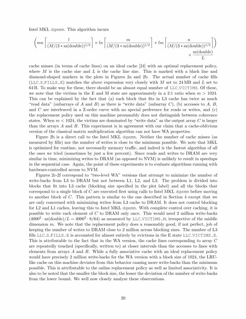
Intel MKL dgemm. This algorithm incurs(mn

⌈l

(M/(3 ∗ sz(double))1/2

⌉+ ln

⌈m


⌉+ lm

⌈n


⌉)× sz(double)

L

cache misses (in terms of cache lines) on an ideal cache [24] with an optimal replacement policy,where M is the cache size and L is the cache line size. This is marked with a black line anddiamond-shaped markers in the plots in Figures 2a and 2b. The actual number of cache fills(LLC S FILLS.E) matches the above expression very closely with M set to 24 MB and L set to64 B. To make way for these, there should be an almost equal number of LLC VICTIMS. Of these,we note that the victims in the E and M state are approximately in a 2:1 ratio when m > 1024.This can be explained by the fact that (a) each block that fits in L3 cache has twice as much“read data” (subarrays of A and B) as there is “write data” (subarray C), (b) accesses to A, B,and C are interleaved in a Z-order curve with no special preference for reads or writes, and (c)the replacement policy used on this machine presumably does not distinguish between coherencestates. When m < 1024, the victims are dominated by “write data” as the output array C is largerthan the arrays A and B. This experiment is in agreement with our claim that a cache-obliviousversion of the classical matrix multiplication algorithm can not have WA properties.

Figure 2b is a direct call to the Intel MKL dgemm. Neither the number of cache misses (asmeasured by fills) nor the number of writes is close to the minimum possible. We note that MKLis optimized for runtime, not necessarily memory traffic, and indeed is the fastest algorithm of allthe ones we tried (sometimes by just a few percent). Since reads and writes to DRAM are verysimilar in time, minimizing writes to DRAM (as opposed to NVM) is unlikely to result in speedupsin the sequential case. Again, the point of these experiments is to evaluate algorithms running withhardware-controlled access to NVM.

Figures 2c-2f correspond to “two-level WA” versions that attempt to minimize the number ofwrite-backs from L3 to DRAM but not between L1, L2, and L3. The problem is divided intoblocks that fit into L3 cache (blocking size specified in the plot label) and all the blocks thatcorrespond to a single block of C are executed first using calls to Intel MKL dgemm before movingto another block of C. This pattern is similar to the one described in Section 4 except that weare only concerned with minimizing writes from L3 cache to DRAM. It does not control blockingfor L2 and L1 caches, leaving this to Intel MKL dgemm. With complete control over caching, it ispossible to write each element of C to DRAM only once. This would need 2 million write-backs(40002 · sz(double)/L = 40002 · 8/64) as measured by LLC VICTIMS.M, irrespective of the middledimension m. We note that the replacement policy does a reasonably good, if not perfect, job ofkeeping the number of writes to DRAM close to 2 million across blocking sizes. The number of L3fills LLC S FILLS.E is accounted for almost entirely by evictions in the E state LLC VICTIMS.E.This is attributable to the fact that in the WA version, the cache lines corresponding to array Care repeatedly touched (specifically, written to) at closer intervals than the accesses to lines withelements from arrays A and B. While a fully associative cache with an ideal replacement policywould have precisely 2 million write-backs for the WA version with a block size of 1024, the LRU-like cache on this machine deviates from this behavior causing more write-backs than the minimumpossible. This is attributable to the online replacement policy as well as limited associativity. It isalso to be noted that the smaller the block size, the lesser the deviation of the number of write-backsfrom the lower bound. We well now closely analyze these observations.

20

6.2 Cache Replacement Policy and Cache Miss Analysis

Background. Most commonly, the cache replacement policy that determines the mapping ofvirtual memory addresses to cache lines seeks to minimize the number of cache misses incurredby the instructions in their execution order. While the optimal mapping [9] is not always possibleto decide in an online setting, the online “least-recently used” (LRU) policy is competitive withthe optimal offline policy [42] in terms of the number of cache misses. Sleator and Tarjan [42]show that for any sequence of instructions (memory accesses), the number of cache misses for theLRU policy on a fully associative cache with M cache lines each of size L is within a factor of(M/(M −M ′ + 1)) of that for the optimal offline policy on a fully associative cache with M ′ lineseach of size L, when starting from an empty cache state. This means that a 2M -size LRU-basedcache incurs at most twice as many misses as a cache of size M with optimal replacement. Thisbound motivates the simplification of the analysis of algorithms on real caches (which is difficult) toan analysis on an “ideal cache model” which uses the optimal offline replacement policy and is fullyassociative [24]. Analysis of a stream of instructions on a single-level ideal cache model yields atheoretical upper bound on the number of cache misses that will be incurred on a multi-level cachewith LRU replacement policy and limited associativity used in many architectures [24]. Therefore,it can be argued that the LRU policy and its theoretical guarantees greatly simplify algorithmicanalysis.

LRU and write-avoidance. The LRU policy does not specifically prioritize the minimization ofwrites to memory. So it is natural to ask if LRU or LRU-like replacement policies can preserve thewrite-avoiding properties we are looking for. In recent work, Blelloch et al. [12] define “AsymmetricIdeal-Cache” and “Asymmetric External Memory” models which have different costs for cacheevictions in the exclusive or modified states. They show [12, Lemma 2.1] that a simple modificationof LRU, wherein one half of the cache lines are reserved for reads and the other half for writes,can be competitive with the asymmetric ideal-cache model. While this clean theoretical guaranteegreatly simplifies algorithmic analysis, the reservation policy is conservative in terms of cache usage.

We argue that the unmodified LRU policy does in fact preserve WA properties for the algorithmsin Section 4, if not for all algorithms, when an appropriate block size is chosen.

Proposition 6.1 If the two-level WA classical matrix multiplication (Cm×n = Am×l ∗ Bl×n) inAlgorithm 1 is executed on a sequential machine with a two-level memory hierarchy, and the blocksize b is chosen so that five blocks of size b-by-b fit in the fast memory with at least one cache lineremaining (5b2 ∗ sz(element) + 1 ≤ M), the number of write-backs to the slow memory caused bythe Least Recently Used (LRU) replacement policy running on a fully associative fast memory ismn irrespective of the order of instructions within the call to the multiplication of individual blocks(the call nested inside the loops).

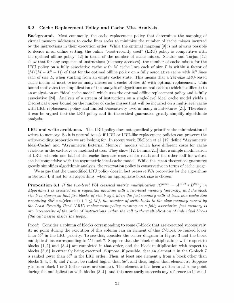
Proof: Consider a column of blocks corresponding to some C-block that are executed successively.At no point during the execution of this column can an element of this C-block be ranked lowerthan 5b2 in the LRU priority. To see this, consider the center diagram in Figure 3 and the blockmultiplications corresponding to C-block 7. Suppose that the block multiplications with respect toblocks 1, 2 and 3, 4 are completed in that order, and the block multiplication with respect toblocks 5, 6 is currently being executed. Suppose, if possible, that an element x in the C-block 7is ranked lower than 5b2 in the LRU order. Then, at least one element y from a block other thanblocks 3, 4, 5, 6, and 7 must be ranked higher than 5b2, and thus, higher than element x. Supposey is from block 1 or 2 (other cases are similar). The element x has been written to at some pointduring the multiplication with blocks 3, 4, and this necessarily succeeds any reference to blocks 1

21

5

3

A

BC

2

4

1

6

7

7

7

5

3

A

BC

2

4

1

6

7

7

7

5

3

A

BC

2

4

1

6

7

7

7

Figure 3: Execution of a column perpendicular to the C-block 7 in classical matrix multiplication.The left and the right diagram correspond to the code in Figures 4a and 4b, respectively. Theircorresponding hardware measurements are in the left and right columns of Figure 5.

and 2 since block multiplication with respect to 1, 2 is completed before the block multiplicationwith 3, 4, which is a contradiction.

So, once a C-block is loaded into fast memory, it is never evicted until the column perpendicularto it is complete, at which point accesses corresponding to the next column induce an evictioncausing a write-back to slow memory. Hence each element of C is written back to slow memoryonly once.

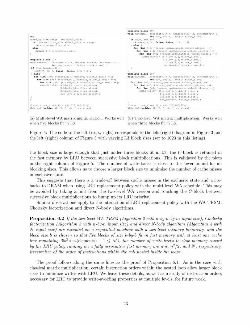
This proposition suggests that the LRU policy does very well at avoiding writes for classicalmatrix multiplication. This claim is validated by plots in Figures 2 and 5 with L3 block size 700(five blocks of size 793 fit in L3). The number of L3 evictions in the modified state is close to thelower bound for all orderings of instructions within the block multiplication that fits in L3 cache.We speculate that the small gap arises because the cache is not perfect LRU (it is a limited-stateapproximation described earlier) and not fully associative.

When fewer than five blocks fit in L3, the multi-level WA algorithm in Figure 4a does poorlyin conjunction with LRU (see left column of Figure 5). This is because large parts of the C-blockcurrently being used have very low LRU priority and get evicted repeatedly. To see this, considerthe left diagram in Figure 3. The block multiplication corresponding to blocks 3, 4 and 7 is orderedby subcolumns. As a result, at the end of this block multiplication, several subblocks of C-blockshave lower LRU priority than the A- and B-surfaces of recently executed subcolumns. When fewerthan five blocks fit in L3, the block multiplication corresponding to input blocks 5, 6 and outputblock 7 forces the eviction of low LRU-priority subblocks of C-block 7 to make space for blocks5 and 6. The larger the block size, the greater the number of write-backs to DRAM. In fact,when the block size is such that just three blocks fit in L3 (1024 for this machine), a constantfraction of C-block is evicted for each block multiplication. This can been seen in the linear trendin L3 VICTIMS.M in the top-left plot in Figure 5. To make LRU work reasonably well at avoidingwrites, we are forced to choose a smaller block size than the maximum possible, incurring morecache misses and fills in the exclusive state (notice that, all other parameters fixed, the number ofLLC S FILLS.E and L3 VICTIMS.E events is higher for smaller block sizes in the left column ofFigure 5).

On the other hand, if we use a WA approach only between L3 and DRAM, these issues can beavoided by executing block multiplications in slabs parallel to the C-block as in the code Figure 4band illustrated in the right diagram in Figure 3. At the end of each block multiplication, thisordering leaves all elements of the C-blocks at a relatively high LRU priority. Therefore, even when

22

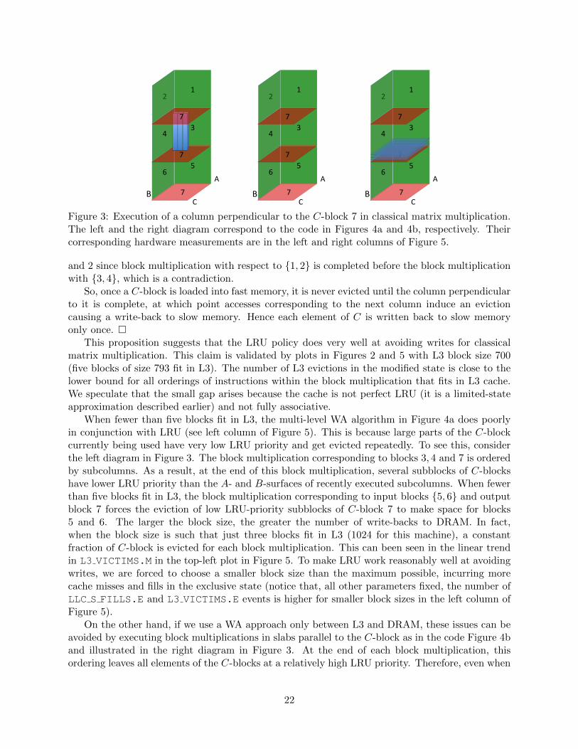
intround_up (int range, int block_size) if ((range/block_size)*block_size == range)

return range/block_size;else

return 1 + range/block_size;

template<class DT>void WAMatMul (denseMat<DT> A, denseMat<DT> B, denseMat<DT> C,

int num_levels, lluint* block_sizes) if (num_levels==1)

mklMM(A, B, C, false, false, 1.0, 1.0); else

for (int i=0; i<round_up(C.numrows,*block_sizes); ++i)for (int k=0; k<round_up(C.numcols,*block_sizes); ++k)

for (int j=0; j<round_up(A.numcols,*block_sizes); ++j)WAMatMul<DT> (A.block(i,j,*block_sizes),

B.block(j,k,*block_sizes),C.block(i,k,*block_sizes),num_levels-1,block_sizes+1);

lluint block_sizes[4] = 0,1023,100,32;WAMatMul<double> (A, B, C, 4, block_sizes);

(a) Multi-level WA matrix multiplication. Works wellwhen five blocks fit in L3.

template<class DT>void ABMatMul (denseMat<DT> A, denseMat<DT> B, denseMat<DT> C,

int num_levels, lluint* block_sizes) if (num_levels==1) mklMM(A, B, C, false, false, 1.0, 1.0);

else for (int j=0; j<round_up(A.numcols,*block_sizes); ++j)

for (int i=0; i<round_up(C.numrows,*block_sizes); ++i)for (int k=0; k<round_up(C.numcols,*block_sizes); ++k)

ABMatMul<DT> (A.block(i,j,*block_sizes),B.block(j,k,*block_sizes),C.block(i,k,*block_sizes),num_levels-1,block_sizes+1);

template<class DT>void WAMatMul (denseMat<DT> A, denseMat<DT> B, denseMat<DT> C,

int num_levels, lluint* block_sizes) for (int i=0; i<round_up(C.numrows,*block_sizes); ++i)for (int k=0; k<round_up(C.numcols,*block_sizes); ++k)

for (int j=0; j<round_up(A.numcols,*block_sizes); ++j)ABMatMul<DT> (A.block(i,j,*block_sizes),

B.block(j,k,*block_sizes),C.block(i,k,*block_sizes),num_levels-1,block_sizes+1);

lluint block_sizes[4] = 0,1023,100,32;WAMatMul<double> (A, B, C, 4, block_sizes);

(b) Two-level WA matrix multiplication. Works wellwhen three blocks fit in L3.

Figure 4: The code to the left (resp., right) corresponds to the left (right) diagram in Figure 3 andthe left (right) column of Figure 5 with varying L3 block sizes (set to 1023 in this listing).

the block size is large enough that just under three blocks fit in L3, the C-block is retained inthe fast memory by LRU between successive block multiplications. This is validated by the plotsin the right column of Figure 5. The number of write-backs is close to the lower bound for allblocking sizes. This allows us to choose a larger block size to minimize the number of cache missesin exclusive state.

This suggests that there is a trade-off between cache misses in the exclusive state and write-backs to DRAM when using LRU replacement policy with the multi-level WA schedule. This maybe avoided by taking a hint from the two-level WA version and touching the C-block betweensuccessive block multiplications to bump up its LRU priority.

Similar observations apply to the interaction of LRU replacement policy with the WA TRSM,Cholesky factorization and direct N-body algorithms.

Proposition 6.2 If the two-level WA TRSM (Algorithm 2 with n-by-n-by-m input size), Choleskyfactorization (Algorithm 3 with n-by-n input size) and direct N-body algorithm (Algorithm 4 withN input size) are executed on a sequential machine with a two-level memory hierarchy, and theblock size b is chosen so that five blocks of size b-by-b fit in fast memory with at least one cacheline remaining (5b2 ∗ sz(elements) + 1 ≤ M), the number of write-backs to slow memory causedby the LRU policy running on a fully associative fast memory are nm, n2/2, and N , respectively,irrespective of the order of instructions within the call nested inside the loops.

The proof follows along the same lines as the proof of Proposition 6.1. As is the case withclassical matrix multiplication, certain instruction orders within the nested loop allow larger blocksizes to minimize writes with LRU. We leave these details, as well as a study of instruction ordersnecessary for LRU to provide write-avoiding properties at multiple levels, for future work.

23


L3_VICTIMS.E 0.6 0.7 1.5 4.2 9.2 18.8 37.5 75.7 153.1

LLC_S_FILLS.E 2.4 2.7 3.6 7 13.8 26.8 52.3 103.9 207.6

Write L.B. 2 2 2 2 2 2 2 2 2

0.1

1

10

100

1000

Blocking Sizes

L3: 1023 L2: 100 L1: 32

128 256 512 1K 2K 4K 8K 16K 32K L3_VICTIMS.M 2 1.8 1.9 2.2 2.5 2.8 3 3.6 4.4

L3_VICTIMS.E 0.4 0.7 1.5 3.8 8.4 16.9 33.9 68 136.4

LLC_S_FILLS.E 2.4 2.8 3.8 6.3 11.2 20.1 37.3 72.1 141.4

Write L.B. 2 2 2 2 2 2 2 2 2

0.1

1

10

100

1000

Blocking Sizes

L3: 1023 L2: 100 L1: 32

128 256 512 1K 2K 4K 8K 16K 32K L3_VICTIMS.M 2 2 1.9 2.2 3.3 5.5 9.1 16.7 33

L3_VICTIMS.E 0.3 0.7 1.6 4.2 10.6 22.1 44.8 90.1 182

LLC_S_FILLS.E 2.4 2.8 3.8 6.8 14.2 28 54.3 107.3 215.7

Write L.B. 2 2 2 2 2 2 2 2 2

0.1

1

10

100

1000

Blocking Sizes

L3: 900 L2: 100 L1: 32

128 256 512 1K 2K 4K 8K 16K 32K L3_VICTIMS.M 2 2 1.9 2 2.3 2.5 2.7 3.1 3.8

L3_VICTIMS.E 0.3 0.7 1.6 4.1 10.1 21.1 42.3 84.8 170.5

LLC_S_FILLS.E 2.4 2.9 3.9 6.5 12.8 24 45.4 88.4 174.9

Write L.B. 2 2 2 2 2 2 2 2 2

0.1

1

10

100

1000

Blocking Sizes

L3: 900 L2: 100 L1: 32


L3_VICTIMS.E 0.4 0.7 1.5 3.9 10.4 21.7 43.4 87.2 176

LLC_S_FILLS.E 2.4 2.8 3.7 6.3 13.6 26.2 49.5 96.5 194.4

Write L.B. 2 2 2 2 2 2 2 2 2

0.1

1

10

100

1000

Blocking Sizes

L3: 800 L2: 100 L1: 32

128 256 512 1K 2K 4K 8K 16K 32K L3_VICTIMS.M 2 2 1.9 2 2.2 2.4 2.5 2.9 3.5

L3_VICTIMS.E 0.3 0.8 1.6 3.9 10.2 21.1 42.3 84.7 170.2

LLC_S_FILLS.E 2.4 2.9 3.8 6.2 12.7 23.8 45.2 88.1 174.3

Write L.B. 2 2 2 2 2 2 2 2 2

0.1

1

10

100

1000

Blocking Sizes

L3: 800 L2: 100 L1: 32

128 256 512 1K 2K 4K 8K 16K 32K L3_VICTIMS.M 2 2.1 1.9 2 2.5 3 3.7 4.8 8

L3_VICTIMS.E 0.3 0.8 1.7 4 11.4 25.6 51.4 102.7 207.4

LLC_S_FILLS.E 2.4 2.8 3.9 6.3 14.2 29 55.5 107.9 216.1

Write L.B. 2 2 2 2 2 2 2 2 2

0.1

1

10

100

1000

Blocking Sizes

L3: 700 L2: 100 L1: 32

128 256 512 1K 2K 4K 8K 16K 32K L3_VICTIMS.M 1.9 2 1.9 1.9 2.1 2.3 2.4 2.8 3.3

L3_VICTIMS.E 0.4 0.8 1.8 4 11.3 25.3 50.9 101.9 204.5

LLC_S_FILLS.E 2.4 2.9 4 6.3 13.8 28 53.7 105.2 208.4

Write L.B. 2 2 2 2 2 2 2 2 2

0.1

1

10

100

1000

Blocking Sizes

L3: 700 L2: 100 L1: 32

Figure 5: L3 cache counter measurements of various execution orders of classical matrix multiplication onIntel Xeon 7560. Plots on the left correspond to multi-level WA instruction orders with different L3 blocksizes (the dimension perpendicular to C array is the outermost loop at each level of recursion). Plots onthe right correspond to versions that are blocked to optimize L3 to DRAM write-backs but not L1 to L2and L2 to L3 write-backs (the dimension perpendicular to C is the outermost loop only at the top levelof recursion but not the lower two levels). All experiments have fixed outer dimensions of 4000 each. Thex-axis corresponds to the middle dimension. The y-axis corresponds to cache events described in Section 6.1,measured in millions of cache lines. Each plot is labeled with the blocking sizes at the three levels of recursion.L1 and L2 block sizes are such that three blocks fit within the caches with about 5-10% space left as margin.

24

7 Parallel WA Algorithms

We consider distributed memory parallel algorithms. There is a large literature on CA distributedmemory algorithms (see [4, 21, 15, 44] and the references therein). In the model used there,communication is measured by the number of words and messages moved into and out of individualprocessors’ local memories along the critical path of the algorithm (under various assumptions likebalanced load and/or balanced memory usage and/or starting with just one copy of the inputdata). So in this model, a read from one processor’s local memory is necessarily a write in anotherprocessor’s local memory. (The number of reads and writes may differ by a modest factor in thecase of broadcasts and reductions, depending on how they are implemented.) In other words, if weare only interested in counting “local memory accesses” without further architectural details, CAand WA are equivalent to within a modest factor.

We may refine this simple architectural model in several ways. First, we assume that theprocessors are homogeneous, that each one has it own (identical) memory hierarchy. We definethree models to analyze:

Model 1: Each processor has a two-level memory hierarchy, labeled L2 (say DRAM) and L1 (saycache). Interprocessor communication is between L2s of different processors. Initially onecopy of all input data is stored in a balanced way across the L2s of all processors.

Model 2: Each processor has a three-level memory hierarchy, labeled L3 (say NVM), L2, and L1.Interprocessor communication is again between L2s of different processors.

Model 2.1: Initially one copy of all input data is stored in a balanced way across the L2s ofall processors.

Model 2.2: Initially one copy of all input data is stored in a balanced way across the L3s ofall processors. In particular, we assume the input data is too large to fit in all the L2s.

We let M1, M2, and M3 be the sizes of L1, L2, and L3 on each processor, resp.For all these models, our goal is to determine lower bounds on communication and identify

or invent algorithms that attain them. In particular, we are most concerned with interprocessorcommunication and writes (and possibly reads) to the lowest level of memory on each processor,since these are the most expensive operations.

First consider Model 1, which is the simplest of the three. Referring back to Section 2, we alsohave a lower bound on writes to L2/reads from L1 equal to the size of the output; assuming memorybalance, this is 1/P -th of the total output for each L2. The literature cited above includes a varietyof lower bounds on interprocessor communication, which (to within a modest factor) means bothreads and writes of L2. Finally, Theorem 1 gives us a lower bound on the number of reads fromL2/writes to L1.

In particular, consider classical dense linear algebra, including matrix multiplication, TRSM,Cholesky, and similar operations. The output size is W1 = n2/P , a lower bound on the numberof writes to L2 (on at least one processor in general, or all processors if memory-balanced). Theresults in [7] provide a lower bound on interprocessor communication of Ω(W2) words moved, whereW2 = n2/

√Pc, and 1 ≤ c ≤ P 1/3 is the number of copies of the input data that the algorithm

can make (so also limited by cn2/P ≤M2). This applies to all processors, assuming load balance.(Reference [15] extends this beyond linear algebra.) And [7] together with Theorem 1 tells us thatthere are Ω(W3) reads from L2/writes to L1, where W3 = (n3/P )/

√M1. In general W1 ≤W2 ≤W3,

with asymptotically large gaps in their values (i.e., when n√P 1).

25

It is natural to ask whether it is possible to attain all three lower bounds, defined by W1, W2

and W3, by (1) using a CA algorithm to minimize interprocessor communication, and so attainingW2, and (2) using a WA algorithm for the computations on a single processor, to try to attain W1

and W3.For example, the many CA algorithms for parallel matrix multiplication that have been devel-

oped over time, including Cannon’s algorithm [13], SUMMA [1, 45], and 2.5D matrix multiplication[20], all perform local matrix multiplications on submatrices, so Algorithm 1 could be used on eachprocessor.

In fact, this does not work. To see why, consider SUMMA: at each of√P steps, n√

P-by- n√

Psubmatrices of A and B are sent to each processor, which multiplies them and adds the productto a locally stored submatrix of C of the same size. Using Algorithm 1, this incurs only n2

P writes

to L2. But this is repeated√P times, for a total of n2

√P

writes to L2, which equals W2 (c = 1 for

SUMMA), and so asymptotically exceeds the lower bound W1.Still, this is likely to be good enough in practice, because the cost (measured in bandwidth or

latency) of the words written to L2 over the network in general greatly exceeds the cost of the wordswritten to L2 from L1. So if the number of words written to L2 from L1 and from the network areboth (roughly) W2, runtime will still be minimized.

It is actually possible to attain all three lower bounds, at the cost of needing much morememory (see the last paragraph of Section 2.1): One again runs SUMMA, but now one stores allsubmatrices of A and B sent to each processor in L2 before doing any computation. In this case,the interprocessor communication W2 is the same. This requires enough memory in L2 to store ann√P

-by-n submatrix of A and an n-by- n√P

submatrix of B, so 2n2/√P words. Then one multiplies

these submatrices by calling Algorithm 1 just once, attaining the lower bound W1 on writes to L2

from L1. As stated in the previous paragraph, this increase in memory size (by a factor of√P ) is

unlikely to result in a significant speedup.Now consider Model 2.1. We could potentially use the same algorithm that optimized com-

munication in Model 1 and simply ignore L3. But using L3 could help, by letting us make morecopies of the data (increase c), and so decrease interprocessor communication. But this will comeat the cost of writing these copies to L3. So whether this is worthwhile will depend on the relativecosts of interprocessor communication and writing to L3. In Section 7.1, we will also develop adetailed performance model of this second algorithm for matrix multiplication, called 2.5DMML3,and compare it to the algorithm that just uses L2, called 2.5DMML2. For simplicity, we comparehere just three of the dominant cost terms of these algorithms.

We let βNW be the time per word to send data over the network (i.e., the reciprocal bandwidth),and similarly let β23 be the time per word to read data from L2 and write it to L3, and let β32be the time per word to read from L3 and write to L2; thus we expect β23 β32. We also let1 ≤ c2 < P 1/3 be the number of copies of the data that we have space for in L2, and c2 < c3 ≤ P 1/3

be the (larger) number of copies that we can fit in L3. With this notation we can say that thedominant bandwidth cost of 2.5DMML2 is

domβcost(2.5DMML2) =2n2√Pc2

βNW

and the dominant bandwidth cost of 2.5DMML3 is

domβcost(2.5DMML3) =2n2√Pc3

(βNW + 1.5β23 + β32)

26

The ratio of these costs is

domβcost(2.5DMML2)

domβcost(2.5DMML3)=

√c3c2

βNWβNW + 1.5β23 + β32

which makes it simple to predict which is faster, given the algorithm and hardware parameters.Finally, consider Model 2.2, where the matrices being multiplied are so large that they only fit

in L3 (again, with 1 ≤ c3 ≤ P 1/3 copies). We now determine a slightly different set of lower boundsagainst which to compare our algorithms. Now W1 = n2/p is a lower bound on writes to L3 (thesize of the output, assuming it is balanced across processors). W2 and W3 are the same as before.Treating L2 (and L1) on one processor as “fast memory” and the local L3 and all remote memoriesas “slow memory”, [7] and Theorem 1 again give us a lower bound on writes to each L2 of Ω(W ′3),where W ′3 = (n3/P )/

√M2, which could come from L3 or the network.

We claim that the lower bounds given by W1 and W2 cannot be simultaneously attained.presentation below of two algorithms below each of which attains just one of these lower bounds.Both algorithms will also attain both lower bounds W3 (on reads from L2/writes to L1) and W ′3(on writes to L2 from either L3 or the network).

Theorem 4 Assume n √P 1 and n2/P M2. If the number of words written to L2 from

the network is a small fraction of W ′3 = (n3/P )/√M2, in particular if the lower bound Ω(W2),

where W2 = n2/√Pc, is attained for some 1 ≤ c ≤ P 1/3, then Ω(n2/P 2/3) words must be written to

L3 from L2. In particular the lower bound W1 = n2/P on writes to L3 from L2 cannot be attained.

Proof: The assumptions n √P 1 and n2/P M2 imply W1 W2 W ′3. If the

number of words written to L2 from the network is a small fraction of W ′3, in particular if theW2 bound is attained, then Ω(W ′3) writes to L2 must come from reading L3. By the Loomis-Whitney inequality [40], the number of multiplications performed by a processor satisfies n3/P ≤√

#As ·#Bs ·#Cs, where #As is the number of distinct entries of A available in L2 sometimeduring execution (and similarly for #Bs and #Cs). Thus n3/P ≤ max(#As,#Bs,#Cs)3/2 orn2/P 2/3 ≤ max(#As,#Bs,#Cs). n2/P 2/3 is asymptotically larger the amount of data O(n2/P )originally stored in L3, so Ω(n2/P 2/3) words must be written to L3.

Now we briefly describe the two algorithms that attain all but one of the lower bounds:2.5DMML3ooL2 (“out of L2”) will attain lower bounds given by W2, W3, and W ′3, andSUMMAL3ooL2 will attain lower bounds given by W1, W3, and W ′3. 2.5DMML3ooL2 will ba-sically implement 2.5DMM, moving all the transmitted submatrices to L3 as they arrive (in sub-submatrices of size M2). SUMMAL3ooL2 will perform the SUMMA algorithm, computing each√M2-by-

√M2 submatrix of C completely in L2 before writing it to L3. Using the same notation

as above, we can compute the dominant bandwidth costs of these two algorithms as

domβcost(2.5DMML3ooL2) =βNWn

2

√Pc3

+β23n

2

√Pc3

+β32n

3

P√M2

(2)

domβcost(SUMMAL3ooL2) =βNWn

3

P√M2

+β23n

2

P+

β32n3

P√M2

(3)

which may again be easily compared given the algorithm and hardware parameters.Section 7.1 describes and analyzes in more detail all the algorithms presented above.Section 7.2 presents algorithms for LU factorization (without pivoting) whose complexity anal-

yses in Model 2.2 are very similar to 2.5DMML3ooL2 and SUMMAL3ooL2. Since Theorem 4 maybe extended to “three-nested loop” algorithms like LU [7], we again do not expect to attain allcommunication lower bounds simultaneously.

Extending the above analyses to parallel shared memory algorithms is future work.

27

7.1 Detailed Analysis of Parallel WA Matrix Multiplication Algorithms

Now we consider the costs of WA matrix multiplication to compute C = A∗B with n-by-n matricesusing P processors in more detail. We will compare the costs of three algorithms which apply toModel 2.1 presented above, i.e., all the data can fit in L2:

2DMML2: 2D matrix multiplication, so using one copy of all the data, using only L2;

2.5DMML2: 2.5D matrix multiplication, replicating the data c2 > 1 times, using only L2;

2.5DMML3: 2.5D matrix multiplication, replicating the data c3 > c2 times, using L3.

In all cases, we assume an initial 2D data layout, with one copy of the data stored in L2, i.e., eachprocessor’s L2 contains an n√

P-by- n√

Psubmatrix of A and B, so 2n2/P words altogether. (For

simplicity we assume all quantities like√P ,√c,√P/c, n/

√P , n/

√P/c, etc., are integers.) This

means that 2.5DMML2 and 2.5DMML3 will need an initial step to transform the input data layoutto the one assumed by 2.5D matrix multiplication [20].

The 2.5D algorithms then proceed in 4 steps. When we use the notation c in a formula, we willlater specialize it to c = c2 for 2.5DMML2 and to c = c3 for 2.5DMML3. The limit on c is c ≤ P 1/3

[6].

1. The processors on the top layer of the√P/c-by-

√P/c-by-c 2.5D processor grid gather all c

n√P

-by- n√P

submatrices of A and B (stored in L2s) to build their own n√P/c

-by- n√P/c

subma-

trices of A and B, stored in their L2s (for 2.5DMML2) or L3s (for 2.5DMML3). Each gatherconsists of c messages of size 2n2/P , so a total of 2n2c/P words and c messages; we assumethat the network topology permits all these gathers to occur simultaneously. Each messagehas a cost as described above, and so this step costs

c2αNW +2n2c2P

βNW (4)

for 2.5DMML2, and

c3(αNW + α23) +2n2c3P

(βNW + β23) (5)

for 2.5DMML3.

At the end of this step, the data is in the format assumed by the 2.5D matrix multiplicationalgorithm in [20], and stored in L2 for 2.5DMML2 and in L3 for 2.5DMML3.

2. We perform step 1 of the 2.5D matrix multiplication algorithm, broadcasting the 2n2c/Pwords owned by each processor on the top layer of the 2.5D processor grid to the other c− 1layers, thus replicating the input data c times. This cannot be done by 2.5DMML3 in asingle broadcast because the message size is limited, so we instead do c3/c2 broadcasts of size2n2c2/P , for the same number of words moved, 2n2c3/P , but about c3/c2 times the numberof messages, 2c3 log2(c3). This raises the cost from

2 log2(c2)

(αNW +

2n2c2P

βNW

)(6)

for 2.5DMML2 to

2c3c2

log2(c3)

(α32 + αNW + α23 +

2n2c2P

(β32 + βNW + β23)

)(7)

28

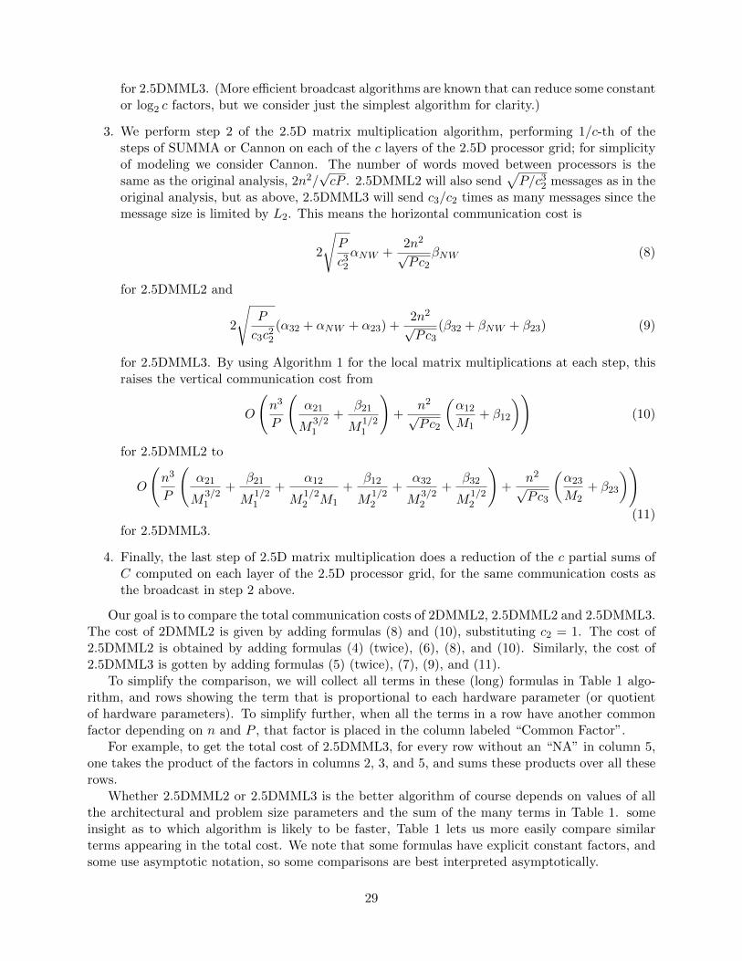
for 2.5DMML3. (More efficient broadcast algorithms are known that can reduce some constantor log2 c factors, but we consider just the simplest algorithm for clarity.)

3. We perform step 2 of the 2.5D matrix multiplication algorithm, performing 1/c-th of thesteps of SUMMA or Cannon on each of the c layers of the 2.5D processor grid; for simplicityof modeling we consider Cannon. The number of words moved between processors is thesame as the original analysis, 2n2/

√cP . 2.5DMML2 will also send

√P/c32 messages as in the

original analysis, but as above, 2.5DMML3 will send c3/c2 times as many messages since themessage size is limited by L2. This means the horizontal communication cost is

2

√P

c32αNW +

2n2√Pc2

βNW (8)

for 2.5DMML2 and

2

√P

c3c22(α32 + αNW + α23) +

2n2√Pc3

(β32 + βNW + β23) (9)

for 2.5DMML3. By using Algorithm 1 for the local matrix multiplications at each step, thisraises the vertical communication cost from

O

(n3

P

(α21

M3/21

+β21

M1/21

)+

n2√Pc2

(α12

M1+ β12

))(10)

for 2.5DMML2 to

O

(n3

P

(α21

M3/21

+β21

M1/21

+α12

M1/22 M1

+β12

M1/22

+α32

M3/22

+β32

M1/22

)+

n2√Pc3

(α23

M2+ β23

))(11)

for 2.5DMML3.

4. Finally, the last step of 2.5D matrix multiplication does a reduction of the c partial sums ofC computed on each layer of the 2.5D processor grid, for the same communication costs asthe broadcast in step 2 above.

Our goal is to compare the total communication costs of 2DMML2, 2.5DMML2 and 2.5DMML3.The cost of 2DMML2 is given by adding formulas (8) and (10), substituting c2 = 1. The cost of2.5DMML2 is obtained by adding formulas (4) (twice), (6), (8), and (10). Similarly, the cost of2.5DMML3 is gotten by adding formulas (5) (twice), (7), (9), and (11).

To simplify the comparison, we will collect all terms in these (long) formulas in Table 1 algo-rithm, and rows showing the term that is proportional to each hardware parameter (or quotientof hardware parameters). To simplify further, when all the terms in a row have another commonfactor depending on n and P , that factor is placed in the column labeled “Common Factor”.

For example, to get the total cost of 2.5DMML3, for every row without an “NA” in column 5,one takes the product of the factors in columns 2, 3, and 5, and sums these products over all theserows.

Whether 2.5DMML2 or 2.5DMML3 is the better algorithm of course depends on values of allthe architectural and problem size parameters and the sum of the many terms in Table 1. someinsight as to which algorithm is likely to be faster, Table 1 lets us more easily compare similarterms appearing in the total cost. We note that some formulas have explicit constant factors, andsome use asymptotic notation, so some comparisons are best interpreted asymptotically.

29

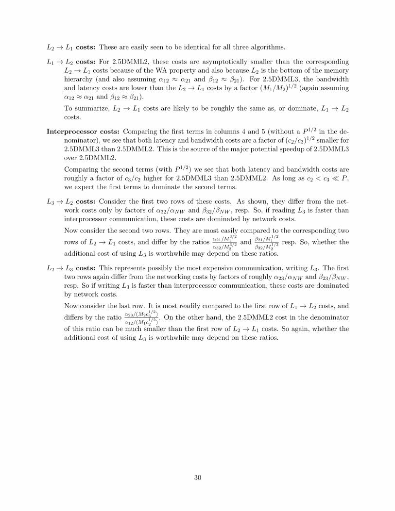
L2 → L1 costs: These are easily seen to be identical for all three algorithms.

L1 → L2 costs: For 2.5DMML2, these costs are asymptotically smaller than the correspondingL2 → L1 costs because of the WA property and also because L2 is the bottom of the memoryhierarchy (and also assuming α12 ≈ α21 and β12 ≈ β21). For 2.5DMML3, the bandwidthand latency costs are lower than the L2 → L1 costs by a factor (M1/M2)

1/2 (again assumingα12 ≈ α21 and β12 ≈ β21).To summarize, L2 → L1 costs are likely to be roughly the same as, or dominate, L1 → L2

costs.

Interprocessor costs: Comparing the first terms in columns 4 and 5 (without a P 1/2 in the de-nominator), we see that both latency and bandwidth costs are a factor of (c2/c3)

1/2 smaller for2.5DMML3 than 2.5DMML2. This is the source of the major potential speedup of 2.5DMML3over 2.5DMML2.

Comparing the second terms (with P 1/2) we see that both latency and bandwidth costs areroughly a factor of c3/c2 higher for 2.5DMML3 than 2.5DMML2. As long as c2 < c3 P ,we expect the first terms to dominate the second terms.

L3 → L2 costs: Consider the first two rows of these costs. As shown, they differ from the net-work costs only by factors of α32/αNW and β32/βNW , resp. So, if reading L3 is faster thaninterprocessor communication, these costs are dominated by network costs.

Now consider the second two rows. They are most easily compared to the corresponding two

rows of L2 → L1 costs, and differ by the ratiosα21/M

3/21

α32/M3/22

andβ21/M

1/21

β32/M1/22

resp. So, whether the

additional cost of using L3 is worthwhile may depend on these ratios.

L2 → L3 costs: This represents possibly the most expensive communication, writing L3. The firsttwo rows again differ from the networking costs by factors of roughly α23/αNW and β23/βNW ,resp. So if writing L3 is faster than interprocessor communication, these costs are dominatedby network costs.

Now consider the last row. It is most readily compared to the first row of L1 → L2 costs, and

differs by the ratioα23/(M2c

1/23 )

α12/(M1c1/22 )

. On the other hand, the 2.5DMML2 cost in the denominator

of this ratio can be much smaller than the first row of L2 → L1 costs. So again, whether theadditional cost of using L3 is worthwhile may depend on these ratios.

30

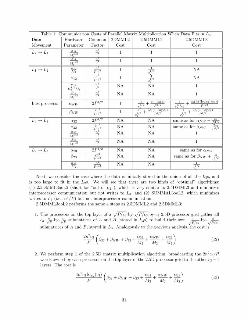
Table 1: Communication Costs of Parallel Matrix Multiplication When Data Fits in L2

Data Hardware Common 2DMML2 2.5DMML2 2.5DMML3Movement Parameter Factor Cost Cost Cost

L2 → L1α21

M3/21

n3

P 1 1 1

β21

M1/21

n3

P 1 1 1

L1 → L2α12M1

n2

P 1/2 1 1

c1/22

NA

β12n2

P 1/2 1 1

c1/22

NA

α12

M1/22 M1

n3

P NA NA 1

β12

M1/22

n3

P NA NA 1

Interprocessor αNW 2P 1/2 1 1

c3/22

+ c2+log c2P 1/2

1

c1/23 c2

+ c3(1+(log c3)/c2))

P 1/2

βNW2n2

P 1/2 1 1

c1/22

+ 2c2(1+log c2)

P 1/21

c1/23

+ 2c3(1+log c3)

P 1/2

L3 → L2 α32 2P 1/2 NA NA same as for αNW − c3P 1/2

β322n2

P 1/2 NA NA same as for βNW − 2c3P 1/2

α32

M3/22

n3

P NA NA 1

β32

M1/22

n3

P NA NA 1

L2 → L3 α23 2P 1/2 NA NA same as for αNWβ23

2n2

P 1/2 NA NA same as for βNW + .5

c1/23

α23M2

n2

P 1/2 NA NA 1

c1/23

Next, we consider the case where the data is initially stored in the union of all the L3s, andis too large to fit in the L2s. We will see that there are two kinds of “optimal” algorithms:(1) 2.5DMML3ooL2 (short for “out of L2”), which is very similar to 2.5DMML3 and minimizesinterprocessor communication but not writes to L3, and (2) SUMMAL3ooL2, which minimizeswrites to L3 (i.e., n2/P ) but not interprocessor communication.

2.5DMML3ooL2 performs the same 4 steps as 2.5DMML2 and 2.5DMML3:

1. The processors on the top layer of a√P/c3-by-

√P/c3-by-c3 2.5D processor grid gather all

c3n√P

-by- n√P

submatrices of A and B (stored in L3s) to build their own n√P/c3

-by- n√P/c3

submatrices of A and B, stored in L3. Analogously to the previous analysis, the cost is

2n2c3P

(β32 + βNW + β23 +

α32

M2+αNWM2

+α23

M2

)(12)

2. We perform step 1 of the 2.5D matrix multiplication algorithm, broadcasting the 2n2c3/Pwords owned by each processor on the top layer of the 2.5D processor grid to the other c3− 1layers. The cost is

4n2c3 log2(c3)

P

(β32 + βNW + β23 +

α32

M2+αNWM2

+α23

M2

)(13)

31

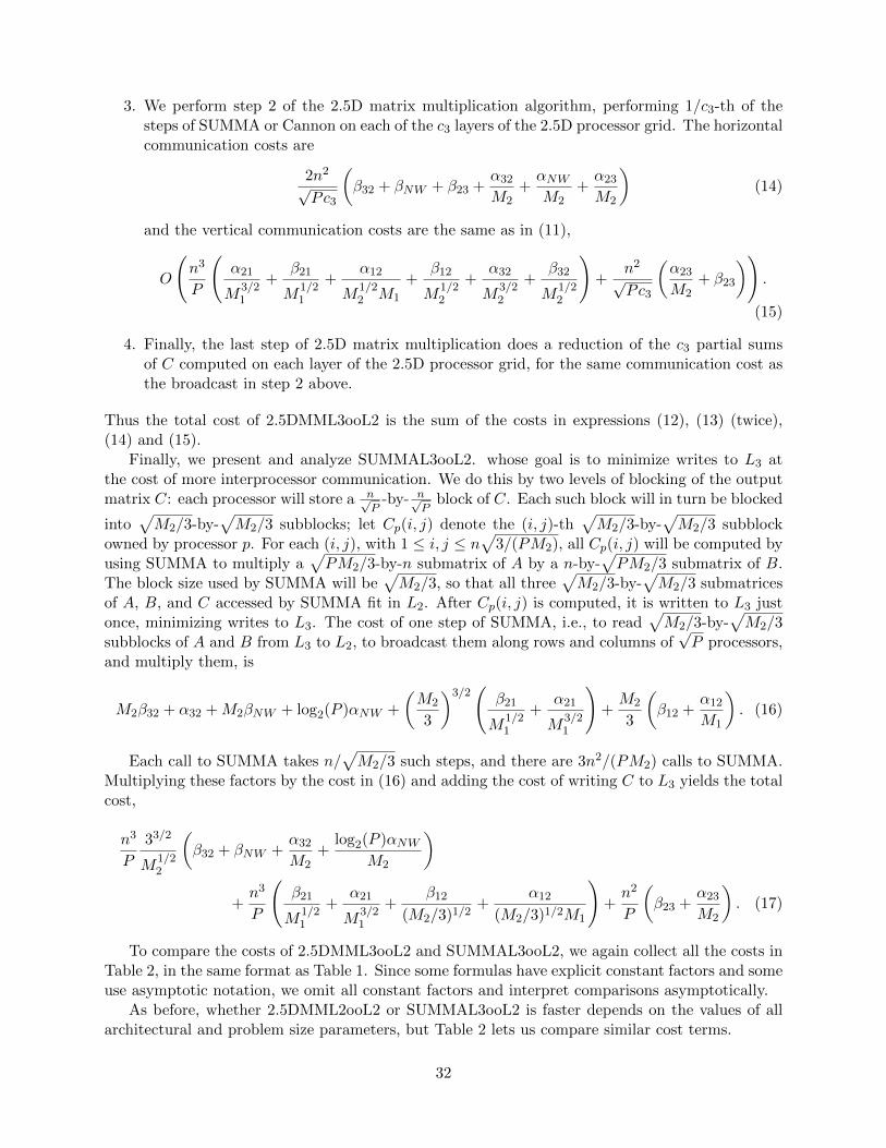
3. We perform step 2 of the 2.5D matrix multiplication algorithm, performing 1/c3-th of thesteps of SUMMA or Cannon on each of the c3 layers of the 2.5D processor grid. The horizontalcommunication costs are

2n2√Pc3

(β32 + βNW + β23 +

α32

M2+αNWM2

+α23

M2

)(14)

and the vertical communication costs are the same as in (11),

O

(n3

P

(α21

M3/21

+β21

M1/21

+α12

M1/22 M1

+β12

M1/22

+α32

M3/22

+β32

M1/22

)+

n2√Pc3

(α23

M2+ β23

)).

(15)

4. Finally, the last step of 2.5D matrix multiplication does a reduction of the c3 partial sumsof C computed on each layer of the 2.5D processor grid, for the same communication cost asthe broadcast in step 2 above.

Thus the total cost of 2.5DMML3ooL2 is the sum of the costs in expressions (12), (13) (twice),(14) and (15).

Finally, we present and analyze SUMMAL3ooL2. whose goal is to minimize writes to L3 atthe cost of more interprocessor communication. We do this by two levels of blocking of the outputmatrix C: each processor will store a n√

P-by- n√

Pblock of C. Each such block will in turn be blocked

into√M2/3-by-

√M2/3 subblocks; let Cp(i, j) denote the (i, j)-th

√M2/3-by-

√M2/3 subblock

owned by processor p. For each (i, j), with 1 ≤ i, j ≤ n√

3/(PM2), all Cp(i, j) will be computed byusing SUMMA to multiply a

√PM2/3-by-n submatrix of A by a n-by-

√PM2/3 submatrix of B.

The block size used by SUMMA will be√M2/3, so that all three

√M2/3-by-

√M2/3 submatrices

of A, B, and C accessed by SUMMA fit in L2. After Cp(i, j) is computed, it is written to L3 justonce, minimizing writes to L3. The cost of one step of SUMMA, i.e., to read

√M2/3-by-

√M2/3

subblocks of A and B from L3 to L2, to broadcast them along rows and columns of√P processors,

and multiply them, is

M2β32 + α32 +M2βNW + log2(P )αNW +

(M2

3

)3/2(

β21

M1/21

+α21

M3/21

)+M2

3

(β12 +

α12

M1

). (16)

Each call to SUMMA takes n/√M2/3 such steps, and there are 3n2/(PM2) calls to SUMMA.

Multiplying these factors by the cost in (16) and adding the cost of writing C to L3 yields the totalcost,

n3

P

33/2

M1/22

(β32 + βNW +

α32

M2+

log2(P )αNWM2

)

+n3

P

(β21

M1/21

+α21

M3/21

+β12

(M2/3)1/2+

α12

(M2/3)1/2M1

)+n2

P

(β23 +

α23

M2

). (17)

To compare the costs of 2.5DMML3ooL2 and SUMMAL3ooL2, we again collect all the costs inTable 2, in the same format as Table 1. Since some formulas have explicit constant factors and someuse asymptotic notation, we omit all constant factors and interpret comparisons asymptotically.

As before, whether 2.5DMML2ooL2 or SUMMAL3ooL2 is faster depends on the values of allarchitectural and problem size parameters, but Table 2 lets us compare similar cost terms.

32

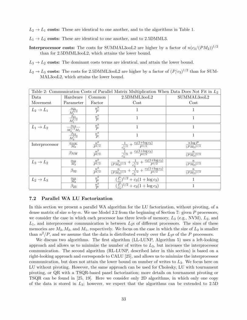
L2 → L1 costs: These are identical to one another, and to the algorithms in Table 1.

L1 → L2 costs: These are identical to one another, and to 2.5DMML3.

Interprocessor costs: The costs for SUMMAL3ooL2 are higher by a factor of n(c3/(PM2))1/2

than for 2.5DMML3ooL2, which attains the lower bound.

L3 → L2 costs: The dominant costs terms are identical, and attain the lower bound.

L2 → L3 costs: The costs for 2.5DMML3ooL2 are higher by a factor of (P/c3)1/2 than for SUM-

MAL3ooL2, which attains the lower bound.

Table 2: Communication Costs of Parallel Matrix Multiplication When Data Does Not Fit in L2

Data Hardware Common 2.5DMML3ooL2 SUMMAL3ooL2Movement Parameter Factor Cost Cost

L2 → L1α21

M3/21

n3

P 1 1

β21

M1/21

n3

P 1 1

L1 → L2α12

M1/22 M1

n3

P 1 1

β12

M1/22

n3

P 1 1

Interprocessor αNWM2

n2

P 1/21

c1/23

+ c3(1+log c3)

P 1/2n logP

(PM2)1/2

βNWn2

P 1/21

c1/23

+ c3(1+log c3)

P 1/2n

(PM2)1/2

L3 → L2α32M2

n2

P 1/2n

(PM2)1/2+ 1

c1/23

+ c3(1+log c3)

P 1/2n

(PM2)1/2

β32n2

P 1/2n

(PM2)1/2+ 1

c1/23

+ c3(1+log c3)

P 1/2n

(PM2)1/2

L2 → L3α23M2

n2

P ( Pc3 )1/2 + c3(1 + log c3) 1

β23n2

P ( Pc3 )1/2 + c3(1 + log c3) 1

7.2 Parallel WA LU Factorization

In this section we present a parallel WA algorithm for the LU factorization, without pivoting, of adense matrix of size n-by-n. We use Model 2.2 from the beginning of Section 7: given P processors,we consider the case in which each processor has three levels of memory, L3 (e.g., NVM), L2, andL1, and interprocessor communication is between L2s of different processors. The sizes of thesememories are M3,M2, and M1, respectively. We focus on the case in which the size of L2 is smallerthan n2/P , and we assume that the data is distributed evenly over the L3s of the P processors.

We discuss two algorithms. The first algorithm (LL-LUNP, Algorithm 5) uses a left-lookingapproach and allows us to minimize the number of writes to L3, but increases the interprocessorcommunication. The second algorithm (RL-LUNP, described later in this section) is based on aright-looking approach and corresponds to CALU [25], and allows us to minimize the interprocessorcommunication, but does not attain the lower bound on number of writes to L3. We focus here onLU without pivoting. However, the same approach can be used for Cholesky, LU with tournamentpivoting, or QR with a TSQR-based panel factorization; more details on tournament pivoting orTSQR can be found in [25, 19]. Here we consider only 2D algorithms, in which only one copyof the data is stored in L3; however, we expect that the algorithms can be extended to 2.5D

33

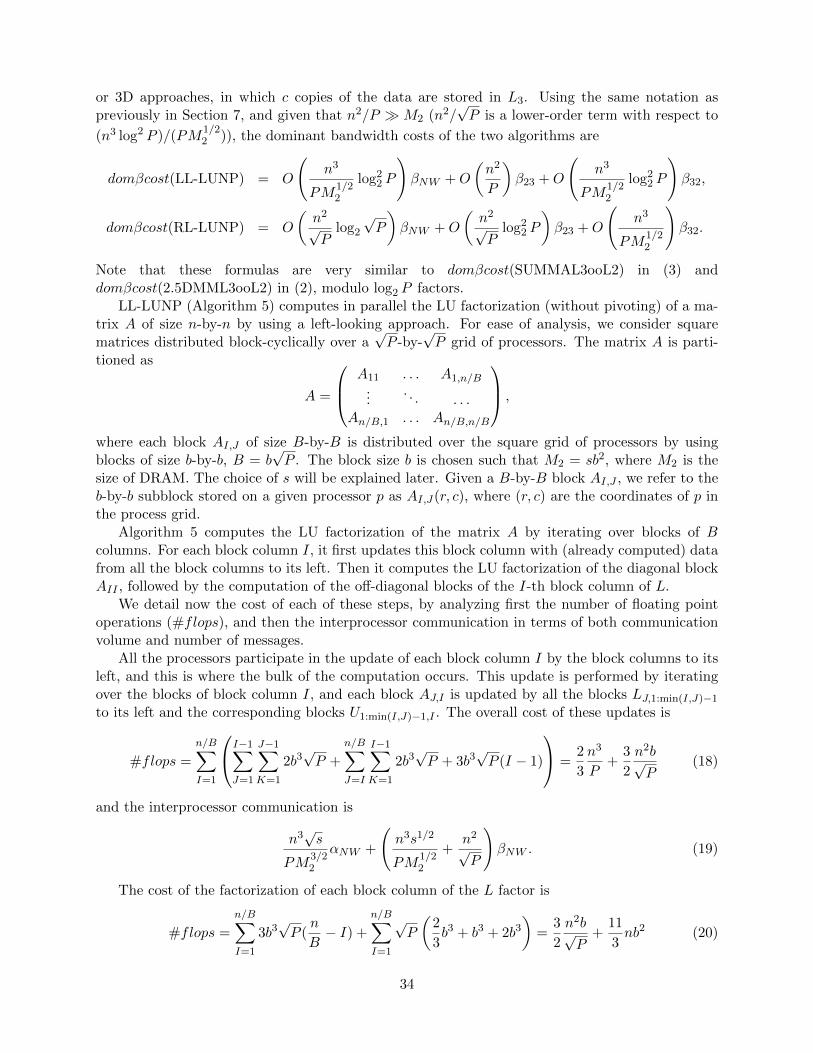
or 3D approaches, in which c copies of the data are stored in L3. Using the same notation aspreviously in Section 7, and given that n2/P M2 (n2/

√P is a lower-order term with respect to

(n3 log2 P )/(PM1/22 )), the dominant bandwidth costs of the two algorithms are

domβcost(LL-LUNP) = O

(n3

PM1/22

log22 P

)βNW +O

(n2

P

)β23 +O

(n3

PM1/22

log22 P

)β32,

domβcost(RL-LUNP) = O

(n2√P

log2√P

)βNW +O

(n2√P

log22 P

)β23 +O

(n3

PM1/22

)β32.

Note that these formulas are very similar to domβcost(SUMMAL3ooL2) in (3) anddomβcost(2.5DMML3ooL2) in (2), modulo log2 P factors.

LL-LUNP (Algorithm 5) computes in parallel the LU factorization (without pivoting) of a ma-trix A of size n-by-n by using a left-looking approach. For ease of analysis, we consider squarematrices distributed block-cyclically over a

√P -by-

√P grid of processors. The matrix A is parti-

tioned as

A =

A11 . . . A1,n/B...

. . . . . .An/B,1 . . . An/B,n/B

,

where each block AI,J of size B-by-B is distributed over the square grid of processors by usingblocks of size b-by-b, B = b

√P . The block size b is chosen such that M2 = sb2, where M2 is the

size of DRAM. The choice of s will be explained later. Given a B-by-B block AI,J , we refer to theb-by-b subblock stored on a given processor p as AI,J(r, c), where (r, c) are the coordinates of p inthe process grid.

Algorithm 5 computes the LU factorization of the matrix A by iterating over blocks of Bcolumns. For each block column I, it first updates this block column with (already computed) datafrom all the block columns to its left. Then it computes the LU factorization of the diagonal blockAII , followed by the computation of the off-diagonal blocks of the I-th block column of L.

We detail now the cost of each of these steps, by analyzing first the number of floating pointoperations (#flops), and then the interprocessor communication in terms of both communicationvolume and number of messages.

All the processors participate in the update of each block column I by the block columns to itsleft, and this is where the bulk of the computation occurs. This update is performed by iteratingover the blocks of block column I, and each block AJ,I is updated by all the blocks LJ,1:min(I,J)−1to its left and the corresponding blocks U1:min(I,J)−1,I . The overall cost of these updates is

#flops =

n/B∑I=1

I−1∑J=1

J−1∑K=1

2b3√P +

n/B∑J=I

I−1∑K=1

2b3√P + 3b3

√P (I − 1)

=2

3

n3

P+

3

2

n2b√P

(18)

and the interprocessor communication is

n3√s

PM3/22

αNW +

(n3s1/2

PM1/22

+n2√P

)βNW . (19)

The cost of the factorization of each block column of the L factor is

#flops =

n/B∑I=1

3b3√P (

n

B− I) +

n/B∑I=1

√P

(2

3b3 + b3 + 2b3

)=

3

2

n2b√P

+11

3nb2 (20)

34

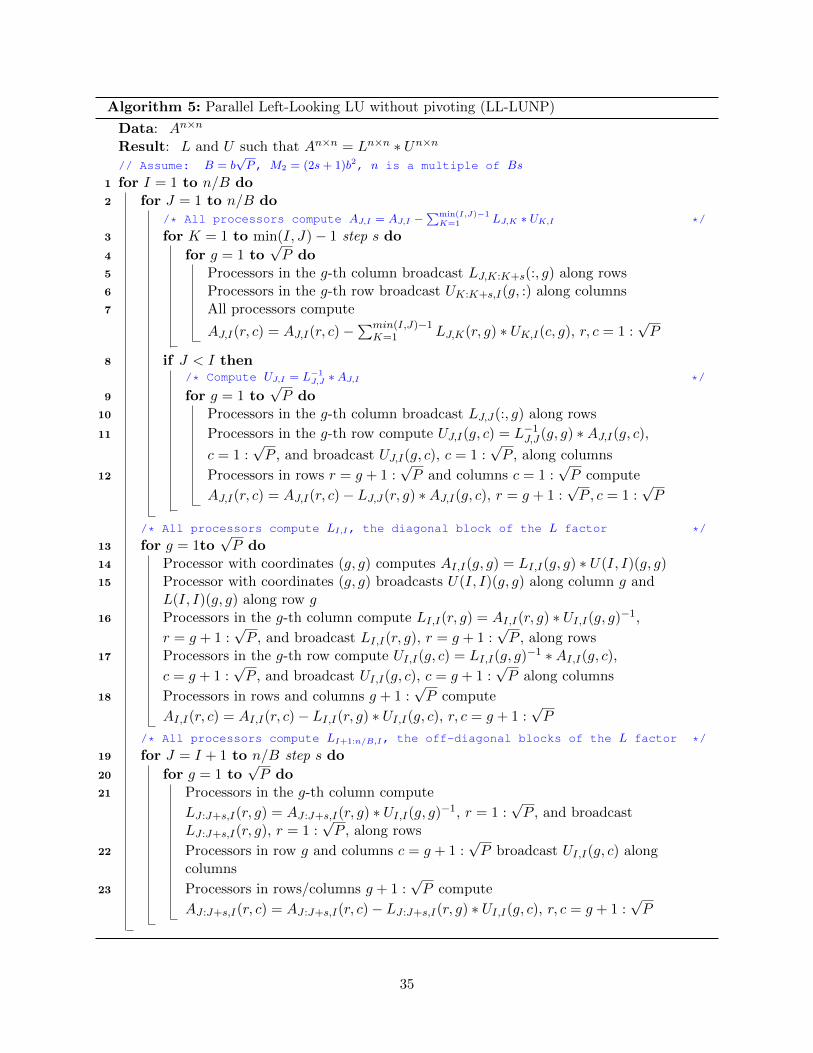
Algorithm 5: Parallel Left-Looking LU without pivoting (LL-LUNP)

Data: An×n

Result: L and U such that An×n = Ln×n ∗ Un×n// Assume: B = b

√P, M2 = (2s+ 1)b2, n is a multiple of Bs

1 for I = 1 to n/B do2 for J = 1 to n/B do

/* All processors compute AJ,I = AJ,I −∑min(I,J)−1

K=1 LJ,K ∗ UK,I */

3 for K = 1 to min(I, J)− 1 step s do

4 for g = 1 to√P do

5 Processors in the g-th column broadcast LJ,K:K+s(:, g) along rows6 Processors in the g-th row broadcast UK:K+s,I(g, :) along columns7 All processors compute

AJ,I(r, c) = AJ,I(r, c)−∑min(I,J)−1

K=1 LJ,K(r, g) ∗ UK,I(c, g), r, c = 1 :√P

8 if J < I then/* Compute UJ,I = L−1

J,J ∗AJ,I */


10 Processors in the g-th column broadcast LJ,J(:, g) along rows

11 Processors in the g-th row compute UJ,I(g, c) = L−1J,J(g, g) ∗AJ,I(g, c),c = 1 :

√P , and broadcast UJ,I(g, c), c = 1 :

√P , along columns

12 Processors in rows r = g + 1 :√P and columns c = 1 :

√P compute

AJ,I(r, c) = AJ,I(r, c)− LJ,J(r, g) ∗AJ,I(g, c), r = g + 1 :√P , c = 1 :

√P

/* All processors compute LI,I, the diagonal block of the L factor */

13 for g = 1to√P do

14 Processor with coordinates (g, g) computes AI,I(g, g) = LI,I(g, g) ∗ U(I, I)(g, g)15 Processor with coordinates (g, g) broadcasts U(I, I)(g, g) along column g and

L(I, I)(g, g) along row g16 Processors in the g-th column compute LI,I(r, g) = AI,I(r, g) ∗ UI,I(g, g)−1,

r = g + 1 :√P , and broadcast LI,I(r, g), r = g + 1 :

√P , along rows

17 Processors in the g-th row compute UI,I(g, c) = LI,I(g, g)−1 ∗AI,I(g, c),c = g + 1 :

√P , and broadcast UI,I(g, c), c = g + 1 :

√P along columns

18 Processors in rows and columns g + 1 :√P compute

AI,I(r, c) = AI,I(r, c)− LI,I(r, g) ∗ UI,I(g, c), r, c = g + 1 :√P

/* All processors compute LI+1:n/B,I, the off-diagonal blocks of the L factor */

19 for J = I + 1 to n/B step s do


21 Processors in the g-th column compute

LJ :J+s,I(r, g) = AJ :J+s,I(r, g) ∗ UI,I(g, g)−1, r = 1 :√P , and broadcast

LJ :J+s,I(r, g), r = 1 :√P , along rows

22 Processors in row g and columns c = g + 1 :√P broadcast UI,I(g, c) along

columns

23 Processors in rows/columns g + 1 :√P compute

AJ :J+s,I(r, c) = AJ :J+s,I(r, c)− LJ :J+s,I(r, g) ∗ UI,I(g, c), r, c = g + 1 :√P

35

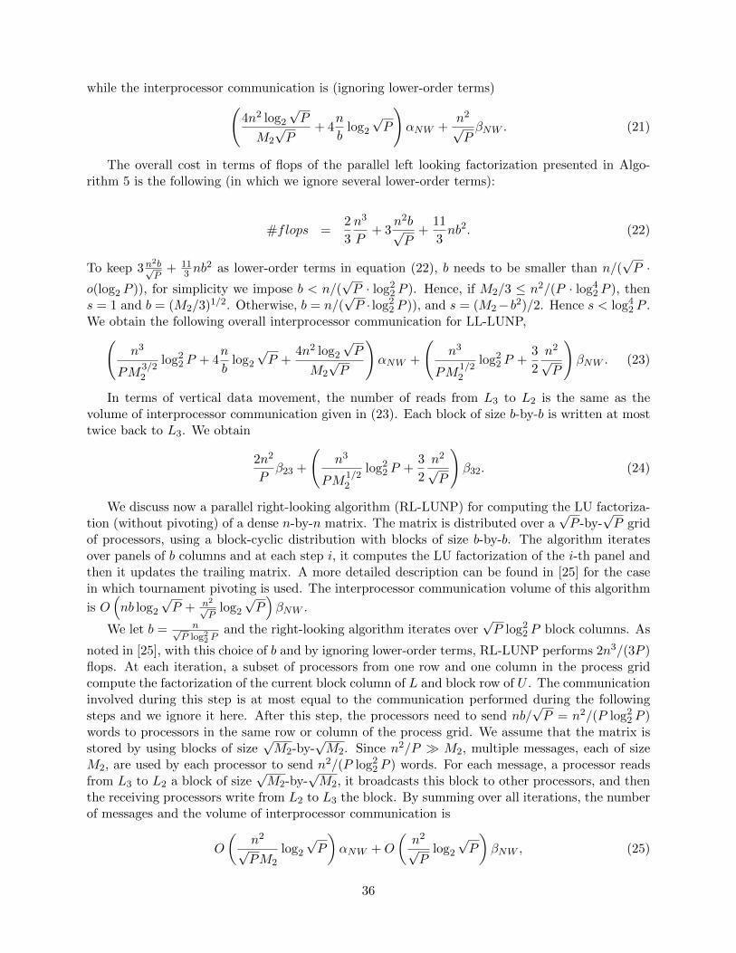
while the interprocessor communication is (ignoring lower-order terms)(4n2 log2

√P

M2

√P

+ 4n

blog2√P

)αNW +

n2√PβNW . (21)

The overall cost in terms of flops of the parallel left looking factorization presented in Algo-rithm 5 is the following (in which we ignore several lower-order terms):

#flops =2

3

n3

P+ 3

n2b√P

+11

3nb2. (22)

To keep 3 n2b√P

+ 113 nb

2 as lower-order terms in equation (22), b needs to be smaller than n/(√P ·

o(log2 P )), for simplicity we impose b < n/(√P · log22 P ). Hence, if M2/3 ≤ n2/(P · log42 P ), then

s = 1 and b = (M2/3)1/2. Otherwise, b = n/(√P · log22 P )), and s = (M2−b2)/2. Hence s < log42 P .

We obtain the following overall interprocessor communication for LL-LUNP,(n3

PM3/22

log22 P + 4n

blog2√P +

4n2 log2√P

M2

√P

)αNW +

(n3

PM1/22

log22 P +3

2

n2√P

)βNW . (23)

In terms of vertical data movement, the number of reads from L3 to L2 is the same as thevolume of interprocessor communication given in (23). Each block of size b-by-b is written at mosttwice back to L3. We obtain

2n2

Pβ23 +

(n3

PM1/22

log22 P +3

2

n2√P

)β32. (24)

We discuss now a parallel right-looking algorithm (RL-LUNP) for computing the LU factoriza-tion (without pivoting) of a dense n-by-n matrix. The matrix is distributed over a

√P -by-

√P grid

of processors, using a block-cyclic distribution with blocks of size b-by-b. The algorithm iteratesover panels of b columns and at each step i, it computes the LU factorization of the i-th panel andthen it updates the trailing matrix. A more detailed description can be found in [25] for the casein which tournament pivoting is used. The interprocessor communication volume of this algorithm

is O(nb log2

√P + n2

√P

log2√P)βNW .

We let b = n√P log22 P

and the right-looking algorithm iterates over√P log22 P block columns. As

noted in [25], with this choice of b and by ignoring lower-order terms, RL-LUNP performs 2n3/(3P )flops. At each iteration, a subset of processors from one row and one column in the process gridcompute the factorization of the current block column of L and block row of U . The communicationinvolved during this step is at most equal to the communication performed during the followingsteps and we ignore it here. After this step, the processors need to send nb/

√P = n2/(P log22 P )

words to processors in the same row or column of the process grid. We assume that the matrix isstored by using blocks of size

√M2-by-

√M2. Since n2/P M2, multiple messages, each of size

M2, are used by each processor to send n2/(P log22 P ) words. For each message, a processor readsfrom L3 to L2 a block of size

√M2-by-

√M2, it broadcasts this block to other processors, and then

the receiving processors write from L2 to L3 the block. By summing over all iterations, the numberof messages and the volume of interprocessor communication is

O

(n2√PM2

log2√P

)αNW +O

(n2√P

log2√P

)βNW , (25)

36

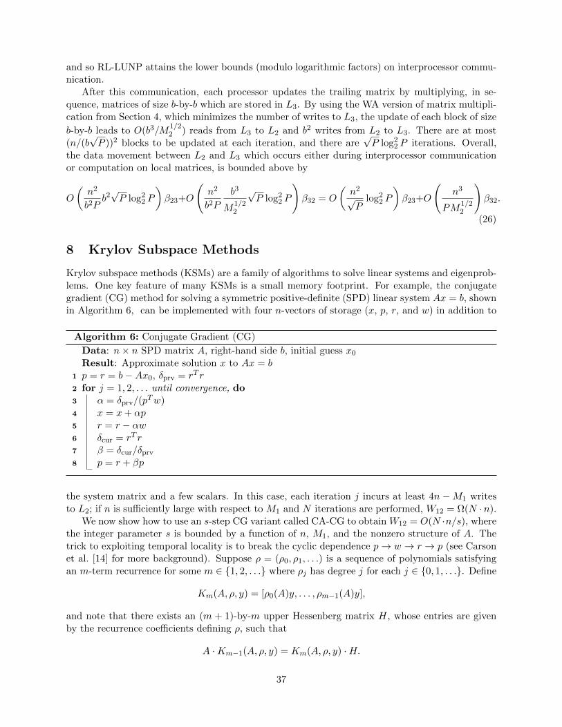
and so RL-LUNP attains the lower bounds (modulo logarithmic factors) on interprocessor commu-nication.

After this communication, each processor updates the trailing matrix by multiplying, in se-quence, matrices of size b-by-b which are stored in L3. By using the WA version of matrix multipli-cation from Section 4, which minimizes the number of writes to L3, the update of each block of size

b-by-b leads to O(b3/M1/22 ) reads from L3 to L2 and b2 writes from L2 to L3. There are at most

(n/(b√P ))2 blocks to be updated at each iteration, and there are

√P log22 P iterations. Overall,

the data movement between L2 and L3 which occurs either during interprocessor communicationor computation on local matrices, is bounded above by

O

(n2

b2Pb2√P log22 P

)β23+O

(n2

b2P

b3

M1/22

√P log22 P

)β32 = O

(n2√P

log22 P

)β23+O

(n3

PM1/22

)β32.

(26)

8 Krylov Subspace Methods

Krylov subspace methods (KSMs) are a family of algorithms to solve linear systems and eigenprob-lems. One key feature of many KSMs is a small memory footprint. For example, the conjugategradient (CG) method for solving a symmetric positive-definite (SPD) linear system Ax = b, shownin Algorithm 6, can be implemented with four n-vectors of storage (x, p, r, and w) in addition to

Algorithm 6: Conjugate Gradient (CG)

Data: n× n SPD matrix A, right-hand side b, initial guess x0Result: Approximate solution x to Ax = b

1 p = r = b−Ax0, δprv = rT r2 for j = 1, 2, . . . until convergence, do3 α = δprv/(p

Tw)4 x = x+ αp5 r = r − αw6 δcur = rT r7 β = δcur/δprv8 p = r + βp

the system matrix and a few scalars. In this case, each iteration j incurs at least 4n −M1 writesto L2; if n is sufficiently large with respect to M1 and N iterations are performed, W12 = Ω(N ·n).

We now show how to use an s-step CG variant called CA-CG to obtain W12 = O(N ·n/s), wherethe integer parameter s is bounded by a function of n, M1, and the nonzero structure of A. Thetrick to exploiting temporal locality is to break the cyclic dependence p→ w → r → p (see Carsonet al. [14] for more background). Suppose ρ = (ρ0, ρ1, . . .) is a sequence of polynomials satisfyingan m-term recurrence for some m ∈ 1, 2, . . . where ρj has degree j for each j ∈ 0, 1, . . .. Define

Km(A, ρ, y) = [ρ0(A)y, . . . , ρm−1(A)y],

and note that there exists an (m + 1)-by-m upper Hessenberg matrix H, whose entries are givenby the recurrence coefficients defining ρ, such that

A ·Km−1(A, ρ, y) = Km(A, ρ, y) ·H.

37

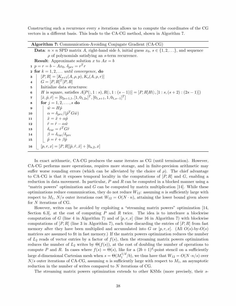
Constructing such a recurrence every s iterations allows us to compute the coordinates of the CGvectors in a different basis. This leads to the CA-CG method, shown in Algorithm 7.

Algorithm 7: Communication-Avoiding Conjugate Gradient (CA-CG)

Data: n× n SPD matrix A, right-hand side b, initial guess x0, s ∈ 1, 2, . . ., and sequenceρ of polynomials satisfying an s-term recurrence.

Result: Approximate solution x to Ax = b1 p = r = b−Ax0, δprv = rT r2 for k = 1, 2, . . . until convergence, do3 [P,R] = [Ks+1(A, ρ, p),Ks(A, ρ, r)]4 G = [P,R]T [P,R]5 Initialize data structures:6 H is square, satisfies A[P (:, 1 : s), R(:, 1 : (s− 1))] = [P,R]H(:, [1 : s, (s+ 2) : (2s− 1)])7 [x, p, r] = [02s+1,1, [1, 01,2s]

T , [01,s+1, 1, 01,s−1]T ]

8 for j = 1, 2, . . . , s do9 w = Hp

10 α = δprv/(pTGw)

11 x = x+ αp12 r = r − αw13 δcur = rTGr14 β = δcur/δprv15 p = r + βp

16 [p, r, x] = [P,R][p, r, x] + [0n,2, x]

In exact arithmetic, CA-CG produces the same iterates as CG (until termination). However,CA-CG performs more operations, requires more storage, and in finite-precision arithmetic maysuffer worse rounding errors (which can be alleviated by the choice of ρ). The chief advantageto CA-CG is that it exposes temporal locality in the computations of [P,R] and G, enabling areduction in data movement. In particular, P and R can be computed in a blocked manner using a“matrix powers” optimization and G can be computed by matrix multiplication [14]. While theseoptimizations reduce communication, they do not reduce W12: assuming n is sufficiently large withrespect to M1, N/s outer iterations cost W12 = O(N · n), attaining the lower bound given abovefor N iterations of CG.

However, writes can be avoided by exploiting a “streaming matrix powers” optimization [14,Section 6.3], at the cost of computing P and R twice. The idea is to interleave a blockwisecomputation of G (line 4 in Algorithm 7) and of [p, r, x] (line 16 in Algorithm 7) with blockwisecomputations of [P,R] (line 3 in Algorithm 7), each time discarding the entries of [P,R] from fastmemory after they have been multiplied and accumulated into G or [p, r, x]. (All O(s)-by-O(s)matrices are assumed to fit in fast memory.) If the matrix powers optimization reduces the numberof L2 reads of vector entries by a factor of f(s), then the streaming matrix powers optimizationreduces the number of L2 writes by Θ(f(s)), at the cost of doubling the number of operations tocompute P and R. In cases where f(s) = Θ(s), like for a (2b + 1)d-point stencil on a sufficiently

large d-dimensional Cartesian mesh when s = Θ(M1/d1 /b), we thus have that W12 = O(N ·n/s) over

N/s outer iterations of CA-CG, assuming n is sufficiently large with respect to M1, an asymptoticreduction in the number of writes compared to N iterations of CG.

The streaming matrix powers optimization extends to other KSMs (more precisely, their s-

38

step variants). For Arnoldi-based KSMs, the computation of G is replaced by a tall-skinny QRfactorization, which can be interleaved with the matrix powers computation in a similar manner.

9 Conclusions and Future Work

Conclusions. Motivated by the fact that writes to some levels of memory can be much moreexpensive than reads (measured in time or energy), for example in the case of nonvolatile memory,we have investigated algorithms that minimize the number of writes. First, we established newlower bounds on the number of writes needed to execute a variety of algorithms. In some cases(e.g., classical linear algebra), these lower bounds are asymptotically smaller than the lower boundon the number of reads, suggesting large savings are possible. We call algorithms that minimize thenumber of reads and writes (i.e., are communication-avoiding (CA)), and also attain asymptoticallysmaller lower bounds on writes, Write-Avoiding (WA) (see Section 2).

In some cases, e.g., the Cooley-Tukey FFT, Strassen’s matrix multiplication algorithm, and,more generally, algorithms whose CDAGs satisfy certain simple conditions on their vertex degrees,the lower bounds on reads and writes differ by at most a modest constant. This implies that WAreorderings of these algorithms cannot exist (see Section 3).

When WA algorithms can exist, we investigated both sequential and distributed memory parallelalgorithms. In the sequential case, we provide WA algorithms for matrix multiplication, triangularsolve, Cholesky factorization, and the direct N-body algorithm. All these algorithms use explicitblocking based on the fast memory size M , and extend to multiple levels of memory hierarchy (seeSection 4).

It is natural to ask whether cache-oblivious algorithms can attain these lower bounds, butwe show this is impossible for direct linear algebra. In other words, a WA algorithm cannot becache-oblivious (see Section 5).

We observed that the explicit movement of cache lines in WA algorithms can be relaxed andreplaced with an online LRU replacement policy. We measured variants of classical matrix mul-tiplication with hardware counters and related the empirical data to theory. These experimentssupport the case for the LRU replacement policy (see Section 6).

In the parallel case, we assumed homogeneous machines, with each processor having an identicallocal memory hierarchy. We analyzed three scenarios (see Section 7).

In the first scenario (called Model 1), the network connects the lowest level of memory on eachprocessor. In this case, the natural approach is to use a CA algorithm to minimize interprocessorcommunication and a WA algorithm locally on each processor to try to minimize writes to thelowest level of memory. While this does reduce the number of local writes to the number of writesfrom the network (which is probably good enough in practice), it does not attain the lower boundwithout using a great deal of extra memory.

In the second scenario (Model 2.1), the network connects the second-lowest level of memory(say DRAM) on each processor, there is another lower, larger level (say NVM), and all the datafits in DRAM, so that it is not necessary to use NVM. Here it may still be advantageous to useNVM to replicate more copies of the data than possible using DRAM alone, in order to reduceinterprocessor communication. We provide a detailed performance model for matrix multiplication,which depends on numerous algorithmic and architectural parameters, that predicts whether usingNVM is helpful.

The third scenario (Model 2.2) differs from the second scenario in that the data is too large to fitin DRAM, and so needs to use NVM. Now we have a lower bound on interprocessor communicationand a lower bound on writes to NVM: we prove that it is impossible to attain both for matrix

39

multiplication, i.e., any algorithm must do asymptotically more of one or the other. We alsopresent two algorithms, each of which attains one of the lower bounds, but not the other. Detailedperformance models are provided that can predict which one is faster. We present analogousalgorithms for LU factorization without pivoting.

Finally, we analyzed iterative linear algebra algorithms (see Section 8) for solving linear systemsAx = b. Prior work on CA Krylov subspace methods (CA-KSMs) showed that under certainconditions on the nonzero structure of A, one could take s steps of the method (requiring s matrix-vector multiplications) for the communication cost of one step, i.e., reading A from DRAM to cacheonce. We show that it is also possible to reduce the number of writes by a factor of s, but at thecost of increasing both the number of reads and the number of arithmetic operations by a factorof at most 2.

Future Work. These results suggest a variety of open problems and future work. In particular,it is natural to try to extend many of the results from Sections 4 through 7 to other linear algebraalgorithms, the direct N-body problem, and more generally algorithms accessing arrays as ana-lyzed in [15]. We conjecture that any WA algorithm for the direct N-body problem (with 2-bodyinteractions) needs to perform twice as many flops as a non-WA algorithm.

In section 7 we showed that no algorithm in Model 2.2 can simultaneously attain both lowerbounds on the number of words communicated over the network, and the number of words writtento L3 from L2, but that there are matmul and LU algorithms that can attain one but not the otherbound. It is natural to ask whether there is a more general lower bound that shows how these twobandwidth quantities tradeoff against one another, and whether there is a family of algorithms thatexhibits this tradeoff.

It is also of interest to investigate WA schedules for shared memory parallel machines. Blellochet al. [12] suggest that previously known thread schedulers that are provably good for various cacheconfigurations are good at minimizing writes in low-depth algorithms [10]. While this covers algo-rithms with polylogarithmic depth such as sorting, the FFT, and classical matrix multiplication, wenote that many linear algebra algorithms (e.g., TRSM and Cholesky) have linear depth. Designinga WA SMP thread scheduler for these algorithms remains an open problem.

We proved that several algorithms can not be reordered to be write-avoiding. It seems thatno WA algorithms exist for certain problems. Specifically, we conjecture that, on a machine witha two-level memory hierarchy with fast memory size M , no algorithm for the Discrete FourierTransform problem or the sorting problem can simultaneously perform o(n logM n) writes to slowmemory and O(n logM n) reads from slow memory (recall that Ω(n logM n) is a lower bound onthe sum of reads and writes for these two problems [3, 28]). Asymptotically fewer writes for theseproblems seem to require an asymptotically greater number of reads.

Finally, if access to NVM is controlled by hardware instead of the programmer, extending theanalysis of Section 6 to the predict the impact of real cache policies on WA algorithms will beimportant to their success in practice.

10 Acknowledgments

We thank Yuan Tang for pointing out the role of write-buffers. We thank U.S. DOE Office ofScience, Office of Advanced Scientific Computing Research, Applied Mathematics Program, grantsDE-SC0010200, DE-SC-0008700, and AC02-05CH11231, for financial support, along with DARPAgrant HR0011-12-2-0016, ASPIRE Lab industrial sponsors and affiliates Intel, Google, Huawei,LG, NVIDIA, Oracle, and Samsung, and MathWorks. Research is supported by grants 1878/14,

40

and 1901/14 from the Israel Science Foundation (founded by the Israel Academy of Sciences andHumanities) and grant 3-10891 from the Ministry of Science and Technology, Israel. Research isalso supported by the Einstein Foundation and the Minerva Foundation. We thank Guy Blellochand Phillip Gibbons for access to the machine on which we ran our experiments.

41

References

[1] R. Agarwal, F. Gustavson, and M. Zubair. A high-performance matrix-multiplication algo-rithm on a distributed-memory parallel computer, using overlapped communication. IBM J.of Research and Development, 38(6):673–681, 1994.

[2] A. Aggarwal, A. K. Chandra, and M. Snir. Communication complexity of PRAMs. TheoreticalComputer Science, 71(1), 1990.

[3] Alok Aggarwal and S. Vitter, Jeffrey. The input/output complexity of sorting and relatedproblems. Commun. ACM, 31(9):1116–1127, September 1988.

[4] G. Ballard, E. Carson, J. Demmel, M. Hoemmen, N. Knight, and O. Schwartz. Acta Numerica,volume 23, chapter Communication lower bounds and optimal algorithms for numerical linearalgebra. Cambridge University Press, 2014.

[5] G. Ballard, J. Demmel, O. Holtz, B. Lipshitz, and O. Schwartz. Graph expansion analysis forcommunication costs of fast rectangular matrix multiplication. In Proc. First MediterraneanConference on Algorithms (MedAlg), pages 13–36, 2012.

[6] G. Ballard, J. Demmel, O. Holtz, B. Lipshitz, and O. Schwartz. Strong scaling of matrix multi-plication algorithms and memory-independent communication lower bounds (brief announce-ment). In 24th ACM Symposium on Parallelism in Algorithms and Architectures (SPAA’12),pages 77–79, 2012.

[7] G. Ballard, J. Demmel, O. Holtz, and O. Schwartz. Minimizing communication in numericallinear algebra. SIAM J. Mat. Anal. Appl., 32(3):866–901, 2011.

[8] G. Ballard, J. Demmel, O. Holtz, and O. Schwartz. Graph expansion and communication costsof fast matrix multiplication. JACM, 59(6), Dec 2012.

[9] L. A. Belady. A study of replacement algorithms for a virtual-storage computer. IBM Syst.J., 5(2):78–101, June 1966.

[10] G. Blelloch, P. Gibbons, and H. Simhadri. Low depth cache-oblivious algorithms. In 22rdACM Symposium on Parallelism in Algorithms and Architectures (SPAA 2010), 2010.

[11] G. Blelloch and R. Harper. Cache and I/O efficient functional algorithms. In 40th ACMSIGPLAN-SIGACT Symposium on Principles of Programming Languages, (POPL 2013),2013.

[12] Guy Blelloch, Jeremy Fineman, Phillip Gibbons, Yan Gu, and Julian Shun. Sorting with asym-metric read and write costs. In ACM Symposium on Parallel Algorithms and Architectures(SPAA 2015), June 2015.

[13] L. Cannon. A cellular computer to implement the Kalman filter algorithm. PhD thesis, Mon-tana State University, Bozeman, MN, 1969.

[14] E. Carson, N. Knight, and J. Demmel. Avoiding communication in nonsymmetric Lanczos-based Krylov subspace methods. SIAM Journal on Scientific Computing, 35(5):S42–S61, 2013.

[15] M. Christ, J. Demmel, N. Knight, T. Scanlon, and K. Yelick. Communication lower boundsand optimal algorithms for programs that reference arrays - part 1. Tech Report UCB/EECS-2013-61, UC Berkeley Computer Science Division, May 2013.

42

[16] National Research Council Committee on Sustaining Growth in Computing Performance. TheFuture of Computing Performance: Game Over or Next Level? National Academies Press,2011. 200 pages, http://www.nap.edu.

[17] F.J. Corbato. A Paging Experiment with the Multics System. Project MAC. Defense TechnicalInformation Center, 1968.

[18] G. De Sandre, L. Bettini, A. Pirola, L. Marmonier, M. Pasotti, M. Borghi, P. Mattavelli,P. Zuliani, L. Scotti, G. Mastracchio, F. Bedeschi, R. Gastaldi, and R. Bez. A 4 Mb LV MOS-Selected Embedded Phase Change Memory in 90 nm Standard CMOS Technology. IEEE J.Solid-State Circuits, 46(1), Jan 2011.

[19] J. Demmel, L. Grigori, M. Hoemmen, and J. Langou. Communication-optimal parallel andsequential QR and LU factorizations. SIAM J. Sci. Comp., 34(1), Feb 2012.

[20] J. Demmel and E. Solomonik. Communication-optimal parallel 2.5D matrix multiplicationand LU factorization algorithms. In EuroPar’11, 2011. report UCB/EECS-2011-72, Jun 2011.

[21] M. Driscoll, E. Georganas, P. Koanantakool, E. Solomonik, and K. Yelick. A communication-optimal n-body algorithm for direct interactions, 2013.

[22] David Eklov, Nikos Nikoleris, David Black-Schaffer, and Erik Hagersten. Cache pirating:Measuring the curse of the shared cache. In Proceedings of the 2011 International Conferenceon Parallel Processing, ICPP ’11, pages 165–175, Washington, DC, USA, 2011. IEEE ComputerSociety.

[23] M. Frigo, C. Leiserson, H. Prokop, and S. Ramachandran. Cache-oblivious algorithms. InProceedings of the 40th IEEE Symposium on Foundations of Computer Science (FOCS 99),pages 285–297, 1999.

[24] Matteo Frigo, Charles E. Leiserson, Harald Prokop, and Sridhar Ramachandran. Cache-oblivious algorithms. In FOCS, 1999.

[25] L. Grigori, J. Demmel, and H. Xiang. CALU: a communication optimal LU factorizationalgorithm. SIAM Journal on Matrix Analysis and Applications, 32:1317–1350, 2011.

[26] J. Hennessy and D. Patterson. Computer Architecture: A Quantitative Approach. MorganKaufmann Publishers, 4th edition, 2007.

[27] Henry. Cache replacement policy for nehalem/snb/ib? http://blog.stuffedcow.net/2013/01/ivb-cache-replacement/, January 2013.

[28] X. Hong and H. T. Kung. I/O complexity: the red blue pebble game. In Proceedings of the13th Symposium on the Theory of Computing, pages 326–334. ACM, 1981.

[29] J. Hu, Q. Zhuge, C. J. Xue, W.-C. Tseng, S. Gu, and E. Sha. Scheduling to optimize cacheutilization for non-volatile main memories. IEEE Trans. Computers, 63(8), Aug 2014.

[30] Intel. Intel(R) Xeon(R) processor 7500 series datasheet, volume 2. http://www.intel.com/content/dam/www/public/us/en/documents/datasheets/xeon-processor-7500-series-vol-2-datasheet.pdf, March 2010.

[31] Intel. Intel(R) Xeon(R) processor 7500 series uncore programming guide. http://www.intel.com/Assets/en_US/PDF/designguide/323535.pdf, March 2010.

43

[32] Intel. Performance Counter Monitor (PCM). http://www.intel.com/software/pcm,2013. Version 2.4.

[33] Intel. Intel(R) 64 and IA-32 architectures optimization reference manual. http://www.intel.com/content/www/us/en/architecture-and-technology/64-ia-32-architectures-optimization-manual.html, September 2014.

[34] Intel. Intel(R) 64 and IA-32 architectures software developer’s man-ual. http://www.intel.com/content/www/us/en/processors/architectures-software-developer-manuals.html, April 2015.

[35] Intel Karla. Cache replacement policy for nehalem/snb/ib? https://communities.intel.com/thread/32695, November 2012.

[36] D. Irony, S. Toledo, and A. Tiskin. Communication lower bounds for distributed-memorymatrix multiplication. J. Parallel Distrib. Comput., 64(9):1017–1026, 2004.

[37] Aamer Jaleel, Kevin B. Theobald, Simon C. Steely, Jr., and Joel Emer. High performance cachereplacement using re-reference interval prediction (rrip). In Proceedings of the 37th AnnualInternational Symposium on Computer Architecture, ISCA ’10, pages 60–71, New York, NY,USA, 2010. ACM.

[38] P. Koanantakool and K. Yelick. A computation- and communication-optimal parallel direct3-body algorithm. In Proceedings of the International Conference for High Performance Com-puting, Networking, Storage and Analysis, SC ’14, pages 363–374, Piscataway, NJ, USA, 2014.IEEE Press.

[39] Adam Litke, Eric Mundon, and Nishanth Aravamudan. libhugetlbfs. http://libhugetlbfs.sourceforge.net, 2006.

[40] L. H. Loomis and H. Whitney. An inequality related to the isoperimetric inequality. Bulletinof the AMS, 55:961–962, 1949.

[41] A. Rasmussen, M. Conley, R. Kapoor, V. T. Lam, G. Porter, and A. Vahdat. Themis: AnI/O Efficient MapReduce. In Proc. ACM Symp. on Cloud Computing (SoCC 2012), San Jose,CA, Oct 2012.

[42] Daniel D. Sleator and Robert E. Tarjan. Amortized efficiency of list update and paging rules.CACM, 28(2), 1985.

[43] M. Snir and S. Graham, editors. Getting up to speed: The Future of Supercomputing. NationalResearch Council, 2004. 227 pages.

[44] A. Tiskin. Communication-efficient parallel generic pairwise elimination. Future GenerationComputer Systems, 23(2):179–188, 2007.

[45] R. van de Geijn and J. Watts. SUMMA: Scalable Universal Matrix Multiplication Algorithm.Concurrency - Practice and Experience, 9(4):255–274, 1997.

44

Documents

Write-Avoiding Algorithms - EECS at UC Berkeley · PDF fileWrite-Avoiding Algorithms Erin ... can aim for is WA algorithms that only write the nal output ... We note that a naive matrix