Embed Size (px)
Citation preview
Parallel Write-Efficient Algorithms and Data Structures forComputational Geometry
Guy E. Blelloch
Carnegie Mellon University
Yan Gu
Carnegie Mellon University
Julian Shun
MIT CSAIL
Yihan Sun
Carnegie Mellon University
ABSTRACTIn this paper, we design parallel write-efficient geometric algo-
rithms that perform asymptotically fewer writes than standard
algorithms for the same problem. This is motivated by emerging
non-volatile memory technologies with read performance being
close to that of random access memory but writes being signifi-
cantly more expensive in terms of energy and latency. We design
algorithms for planar Delaunay triangulation, k-d trees, and static
and dynamic augmented trees. Our algorithms are designed in
the recently introduced Asymmetric Nested-Parallel Model, which
captures the parallel setting in which there is a small symmetric
memory where reads and writes are unit cost as well as a large
asymmetric memory where writes are ω times more expensive
than reads. In designing these algorithms, we introduce several
techniques for obtaining write-efficiency, including DAG tracing,
prefix doubling, and α-labeling, which we believe will be useful for
designing other parallel write-efficient algorithms.
ACM Reference Format:Guy E. Blelloch, Yan Gu, Julian Shun, and Yihan Sun. 2018. Parallel Write-
Efficient Algorithms and Data Structures for Computational Geometry. In
SPAA ’18: 30th ACM Symposium on Parallelism in Algorithms and Architec-tures, July 16–18, 2018, Vienna, Austria. ACM, New York, NY, USA, 12 pages.
https://doi.org/10.1145/3210377.3210380
1 INTRODUCTIONIn this paper, we design a set of techniques and parallel algorithms to
reduce the number of writes to memory as compared to traditional
algorithms. This is motivated by the recent trends in computer
memory technologies that promise byte-addressability, good read
latencies, significantly lower energy and higher density (bits per
area) compared to DRAM. However, one characteristic of these
memories is that reading frommemory is significantly cheaper than
writing to it. Based on projections in the literature, the asymmetry
is between 5–40 in terms of latency, bandwidth, or energy. Roughly
speaking, the reason for this asymmetry is that writing to memory
requires a change to the state of the material, while reading only
requires detecting the current state. This trend poses the interesting
question of how to design algorithms that are more efficient than
traditional algorithms in the presence of read-write asymmetry.
Permission to make digital or hard copies of all or part of this work for personal or
classroom use is granted without fee provided that copies are not made or distributed
for profit or commercial advantage and that copies bear this notice and the full citation
on the first page. Copyrights for components of this work owned by others than ACM
must be honored. Abstracting with credit is permitted. To copy otherwise, or republish,
to post on servers or to redistribute to lists, requires prior specific permission and/or a
fee. Request permissions from [email protected].
SPAA ’18, July 16–18, 2018, Vienna, Austria© 2018 Association for Computing Machinery.
ACM ISBN 978-1-4503-5799-9/18/07. . . $15.00
https://doi.org/10.1145/3210377.3210380
There has been recent research studying models and algorithms
that account for asymmetry in read and write costs [7, 8, 13, 14, 19,
20, 26, 27, 34, 42, 52, 53]. Blelloch et al. [8, 13, 14] propose models in
which writes to the asymmetric memory costω ≥ 1 and all other op-
erations are unit cost. The Asymmetric RAM model [8] has a small
symmetric memory (a cache) that can be used to hold temporary
values and reduce the number of writes to the large asymmetric
memory. The Asymmetric NP (Nested Parallel) model [14] is the
corresponding parallel extension that allows an algorithm to be
scheduled efficiently in parallel, and is the model that we use in
this paper to analyze our algorithms.
Write-efficient parallel algorithms have been studied for many
classes of problems including graphs, linear algebra, and dynamic
programming. However, parallel write-efficient geometric algo-
rithms have only been developed for the 2D convex hull prob-
lem [8]. Achieving parallelism (polylogarithmic depth) and optimal
write-efficiency simultaneously seems generally hard for many
algorithms and data structures in computational geometry. Here,
optimal write-efficiency means that the number of writes that the
algorithm or data structure construction performs is asymptotically
equal to the output size. In this paper, we propose two general
frameworks and show how they can be used to design algorithms
and data structures from geometry with high parallelism as well as
optimal write-efficiency.
The first framework is designed for randomized incremental
algorithms [21, 39, 45]. Randomized incremental algorithms are rel-
atively easy to implement in practice, and the challenge is in simulta-
neously achieving high parallelism and write-efficiency. Our frame-
work consists of two components: a DAG-tracing algorithm and a
prefix doubling technique. We can obtain parallel write-efficient
randomized incremental algorithms by applying both techniques
together. The write-efficiency is from the DAG-tracing algorithm,
that given a current configuration of a set of objects and a new
object, finds the part of the configuration that “conflicts” with the
new object. Finding n objects in a configuration of size n requires
O(n logn) reads but only O(n) writes. Once the conflicts have beenfound, previous parallel incremental algorithms (e.g. [15]) can be
used to resolve the conflicts among objects taking linear reads and
writes. This allows for a prefix doubling approach in which the
number of objects inserted in each round is doubled until all objects
are inserted.
Using this framework, we obtain parallel write-efficient algo-
rithms for comparison sort, planar Delaunay triangulation, and k-dtrees, all requiring optimal work, linear writes, and polylogarithmic
depth. The most interesting result is for Delaunay triangulation
(DT). Although DT can be solved in optimal time and linear writes
sequentially using the plane sweep method [14], previous parallel
DT algorithms seem hard to make write-efficient. Most are based
on divide-and-conquer, and seem to inherently require Θ(n logn)writes. Here we use recent results on parallel randomized incremen-
tal DT [15] and apply the above mentioned approach. For compari-
son sort, our new algorithm is stand-alone (i.e., not based on other
complicated algorithms like Cole’s mergesort [13, 22]). Due to space
constraints, this algorithm is presented in the full version of this
paper [16]. For k-d trees, we introduce the p-batched incremental
construction technique that maintains the balance of the tree while
asymptotically reducing the number of writes.
The second framework is designed for augmented trees, includ-
ing interval trees, range trees, and priority search trees. Our goal
is to achieve write-efficiency for both the initial construction as
well as future dynamic updates. The framework consists of two
techniques. The first technique is to decouple the tree construction
from sorting, and introduce parallel algorithms to construct the
trees in linear reads and writes after the objects are sorted (the sort-
ing can be done with linear writes [13]). Such algorithms provide
write-efficient constructions of these data structures, but can also
be applied in the rebalancing scheme for dynamic updates—once
a subtree is unbalanced, we reconstruct it. The second technique
is α-labeling. We subselect some tree nodes as critical nodes, and
maintain part of the augmentation only on these nodes. By doing
so, we can limit the number of tree nodes that need to be written
on each update, at the cost of having to read more nodes.1
Using this framework, we obtain efficient augmented trees in
the asymmetric setting. In particular, we can construct the trees in
optimal work and writes, and polylogarithmic depth. For dynamic
updates, we provide a trade-off between performing extra reads in
queries and updates, while doing fewer writes on updates. Standard
algorithms useO(logn) reads andwrites per update (O(log2 n) readson a 2D range tree). We can reduce the number of writes by a factor
of Θ(logα) for α ≥ 2, at a cost of increasing reads by at most a
factor of O(α) in the worst case. For example, when the number of
queries and updates are about equal, we can improve the work by
a factor of Θ(logω), which is significant given that the update and
query costs are only logarithmic.
The contributions of this paper are new parallel write-efficient
algorithms for comparison sorting, planar Delaunay triangulation,
k-d trees, and static and dynamic augmented trees (including inter-
val trees, range trees and priority search trees). We introduce two
general frameworks to design such algorithms, which we believe
will be useful for designing other parallel write-efficient algorithms.
2 PRELIMINARIES2.1 Computation ModelsNested-parallel model. The algorithms in this paper is based on
the nested-parallel model where a computation starts and ends with
a single root task. Each task has a constant number of registers,
and runs a standard instruction set from a random access machine,
except it has one additional instruction called FORK. The FORK
instruction takes an integern′ and createsn′ child tasks, which can
run in parallel. Child tasks get a copy of the parent’s register values,
with one special register getting an integer from 1 to n′ indicating
1At a very high level, the α -labeling is similar to the weight-balanced B-tree (WBB
tree) proposed by Arge et al. [4, 5], but there are many differences and we discuss
them in Section 6.
which child it is. The parent task suspends until all its children finish
at which point it continues with the registers in the same state as
when it suspended, except the program counter advanced by one.
We say that a computation has binary branching if n′ = 2. In the
model, a computation can be viewed as a (series-parallel) DAG in
the standard way. We assume every instruction has a weight (cost).
The work (W ) is the sum of the weights of the instructions, and
the depth (D) is the weight of the heaviest path.
Asymmetric NP (Nested Parallel) model.We use the Asymmet-
ric NP (Nested Parallel) model [8], which is the asymmetric version
of the nested-parallel model, to measure the cost of an algorithm
in this paper. The memory in the Asymmetric NP model consists
of (i) an infinitely large asymmetric memory (referred to as large-
memory) accessible to all processors and (ii) a small private sym-metric memory (small-memory) accessible only to one processor.
The cost of writing to large memory is ω, and all other operations
have unit cost. The size of the small-memory is measured in words.
In this paper, we assume the small memory can store a logarithmic
number of words, unless specified otherwise. A more precise and
detailed definition of the Asymmetric NP model is given in [8].
The work W of a computation is the sum of the costs of the
operations in the DAG, which is similar to the symmetric version
but just has extra charges for writes. The depth D is the sum of
the weights on the heaviest path in the DAG. Since the depth can
vary by a logarithmic factor based on specifics of the model (e.g.
allowing binary or multiway branching), in this paper we show
O(ω · polylog(n)) bounds for the depth of the algorithms, disregard-
ing the particular power in the logarithm. Under mild assumptions,
a work-stealing scheduler can execute an algorithm with workWand depth ω · polylog(n) inW /P +O(ω · polylog(n)) expected time
on P processors [8]. We assume concurrent-read, and concurrent-
writes use priority-writes to resolve conflicts. In our algorithm
descriptions, the number of writes refers only to the writes to the
large-memory, and does not include writes to the small-memory.
All reads and writes are to words of size Θ(logn)-bits for an input
size of n.
2.2 Write-Efficient Geometric AlgorithmsSorting and searching are widely used in geometry applications.
Sorting requiresO(ωn+n logn)work andO(ω·polylog(n)) depth [13].Red-black trees with appropriate rebalancing rules require O(ω +logn) amortized work per update (insertion or deletion) [51].
These building blocks facilitate many classic geometric algo-
rithms. The planar convex-hull problem can be solved by first sort-
ing the points by x coordinates and then using Graham’s scan that
requires O(ωn) work [24]. This scan step can be parallelized with
O(ω · polylog(n)) depth [28]. The output-sensitive version uses
O(n logh + ωn log logh) work and O(ω polylog(n)) depth where his the number of points on the hull [8].
3 GENERAL TECHNIQUES FORINCREMENTAL ALGORITHMS
In this section, we first introduce our framework for randomized
incremental algorithms. Our goal is to have a systematic approach
for designing geometric algorithms that are highly parallel and
write-efficient.
Our observation is that it should be possible to make random-
ized incremental algorithms write-efficient since each newly added
object on expectation only conflicts with a small region of the cur-
rent configuration. For instance, in planar Delaunay triangulation,
when a randomly chosen point is inserted, the expected number
of encroached triangles is 6. Therefore, resolving such conflicts
only makes minor modifications to the configuration during the
randomized incremental constructions, leading to algorithms using
fewer writes. The challenges are in finding the conflicted region of
each newly added object write-efficiently and work-efficiently, and
in adding multiple objects into the configuration in parallel without
affecting write-efficiency. We will discuss the general techniques
to tackle these challenges based on the history graph [18, 31], and
then discuss how to apply them to develop parallel write-efficient
algorithms for planar Delaunay triangulation in Section 4 and k-dtree construction in Section 5. The application of these techniques
to designing a write-efficient parallel comparison sorting algorithm
is presented in the full version of this paper [16].
3.1 DAG TracingWe now discuss how to find the conflict set of each newly added
object (i.e., only output the conflict primitives) based on a history
(directed acyclic) graph [18, 31] in a parallel and write-efficient fash-
ion. Since the history graphs for different randomized incremental
algorithms can vary, we abstract the process as a DAG tracing prob-
lem that finds the conflict primitives in each step by following the
history graph.
Definition 3.1 (DAG tracing problem). The DAG tracing problem
takes an element x , a DAGG = (V ,E), a root vertex r ∈ V with zero
in-degree, and a boolean predicate function f (x ,v). It computes
the vertex set S(G,x) = v ∈ V | f (x ,v) and out-degree(v) = 0.
We call a vertex v visible if f (x ,v) is true.
Definition 3.2 (tracable property). We say that the DAG tracing
problem has the tracable property when v ∈ V is visible only if
there exists at least one direct predecessor vertex u of v that is
visible.
Variable Description
D(G) the length of the longest path in GR(G,x) the set of all visible vertices in GS(G,x) the output set of vertices
Theorem 3.3. The DAG tracing problem can be solved inO(|R(G,x)|)work, O(D(G)) depth and O(|S(G,x)|) writes when the problem hasthe tracable property, each vertexv ∈ V has a constant degree, f (x ,v)can be evaluated in constant time, and the small-memory has sizeO(D(G)). Here R(G,x), D(G), and S(G,x) are defined in the previoustable.
Proof. Wefirst discuss a sequential algorithm usingO(|R(G,x)|)work and O(|S(G,x)|) writes. Because of the tracable property, wecan use an arbitrary search algorithm to visit the visible nodes,
which requires O(R(G,x)) writes since we need to mark whether a
vertex is visited or not. However, this approach is not write-efficient
when |S | = o(|R(G,x)|), and we now propose a better solution.
Assume that we give a global ordering ≺v of the vertices in G(e.g., using the vertex labels) and use the following rule to traverse
the visible nodes based on this ordering: a visible node v ∈ V is
visited during the search of its direct visible predecessor u that has
the highest priority among all visible direct predecessors ofv . Basedon this rule, we do not need to store all visited vertices. Instead,
when we visit a vertex v via a directed edge (u,v) from u, we cancheck if u has the highest priority among all visible predecessors
of v . This checking has constant cost since v has a constant degree
and we assume the visibility of a vertex can be verified in constant
time. As long as we have a small-memory of size O(D(G)) thatkeeps the recursion stack and each vertex in V has a constant in-
degree, we can find the output set S(G,x) using O(|R(G,x)|) workand O(|S(G,x)|) writes.
We note that the search tree generated under this rule is unique
and deterministic. Therefore, this observation allows us to traverse
the tree in parallel and in a fork-joinmanner: we can simultaneously
fork off an independent task for each outgoing edges of the current
vertex, and all these tasks can be run independently and in parallel.
The parallel depth, in this case, is upper bounded by O(D(G)), thedepth of the longest path in the graph.
Here we assume the graph is explicitly stored and accessible, so
we slightly modify the algorithms to generate the history graph,
which is straightforward in all cases in this paper.
3.2 The Prefix-Doubling ApproachThe sequential version of randomized incremental algorithms pro-
cess one object (e.g., a point or vertex) in one iteration. The prefix-
doubling approach splits an algorithm into multiple rounds, with
the first round processing one iteration and each subsequent round
doubling the number of iterations processed. This high-level idea
is widely used in parallel algorithm design. We show that the
prefix-doubling approach combined with the DAG tracing algo-
rithm can reduce the number of writes by a factor of Θ(logn) in a
number of algorithms. In particular, our variant of prefix doubling
first processes n/logn iterations using a standard write-inefficient
approach (called as the initial round). Then the algorithm runs
O(log logn) incremental rounds, where the i’th round processes
the next 2i−1n/logn iterations.
4 PLANAR DELAUNAY TRIANGULATIONA Delaunay triangulation (DT) in the plane is a triangulation of a
set of points P such that no point in P is inside the circumcircle of
any triangle (the circle defined by the triangle’s three corner points).
We say a point encroaches on a triangle if it is in the triangle’s
circumcircle, so the triangle will be replaced once this point is added
to the triangulation. We assume for simplicity that the points are
in general position (no three points on a line or four points on a
circle).
Delaunay triangulation is widely studied due to its importance in
many geometry applications. Without considering the asymmetry
between reads and writes, it can be solved sequentially in opti-
mal Θ(n logn) work. It is relatively easy to generate a sequential
write-efficient version that does Θ(n logn) reads and only requires
Θ(n) writes based on the plane sweep method [14]. There are sev-
eral work-efficient parallel algorithms that run in polylogarithmic
depth [6, 15, 17, 44]. More practical ones (e.g., [18, 31]) have linear
depth. Unfortunately, none of them perform any less thanΘ(n logn)
Algorithm 1: ParIncrementalDTInput: A sequence V = v1, . . . ,vn of points in the plane.
Output: The Delaunay triangulation of V .
Maintains: E(t), the points that encroach on each triangle t .
1 tb ← a sufficiently large bounding triangle
2 E(tb ) ← V3 M ← tb 4 while E(t) , ∅ for any t ∈ M do5 parallel foreach triangle t ∈ M do6 Let t1, t2, t3 be the three neighboring triangles7 if min(E(t)) ≤ min(E(t1) ∪ E(t2) ∪ E(t3)) then8 ReplaceTriangle(M, t ,min(E(t)))9 returnM
10 function ReplaceTriangle(M ,t ,v)11 foreach edge (u,w) ∈ t (three of them) do12 if (u,w) is a boundary of v’s encroached region then13 to ← the other triangle sharing (u,w)14 t ′ ← (u,w,v)15 E(t ′) ← v ′ ∈ E(t) ∪ E(to ) | inCircle(v
′, t ′)16 M ← M ∪ t ′17 M ← M \ t
writes. In particular the divide-and-conquer algorithms [6, 17] seem
to inherently require Θ(n logn) writes since the divide or merge
step requires generating an output of size Θ(n), and is applied for
Θ(logn) levels. The randomized incremental approach of Blelloch
et al. (BGSS) [15], which improves the Boissonnat and Teillaud
algorithm [18] to polylogarithmic depth, also requires O(n logn)writes for reasons described below.
In this section, we show how to modify the BGSS algorithm to
use only a linear number of writes, while maintaining the expected
Θ(n logn) bound on work, and polylogarithmic depth. Algorithm 1
shows the pseudocode for the BGSS algorithm. In the algorithm,
the vertices are labeled from 1 to n and when taking a min over
vertices (Lines 7–8) it is with respect to these labels. The algorithm
proceeds in rounds the algorithm adds some triangles (Line 16) and
removes others (Line 17) in each round.
In the algorithm, there are dependences between triangles so that
some of them need to be processed before the other triangles can
proceed. For a sequence of points V , BGSS define the dependencegraphGT (V ) = (T ,E) for the algorithm in the following way. The
vertices T correspond to triangles created by the algorithm, and
for each call to ReplaceTriangle(M, t ,vi ), we place an arc from
triangle t and its three neighbors (t1, t2, and t3) to each of the one,
two, or three triangles created by ReplaceTriangle. Every triangle
T with depth d(T ) in GT (V ) is created by the algorithm in round
d(T ). BGSS show that for a randomly ordered set of input points
of size n, the depth of the dependence graph is O(logn) whp2, andhence the algorithm runs in O(logn) rounds whp. Each round can
be done in O(logn) depth giving an overall depth of O(log2 n) whpon the nested-parallel model.
The algorithm, however, is not write-efficient. In particular, every
point moves down the DAG through the rounds (on line 15), and
therefore can be moved O(logn) times, each requiring a write.
2We sayO (f (n)) with high probability (whp) to indicateO (c · f (n)) with probability
to be at least 1 − 1/nc for any constant c > 0.
𝑣
𝐴
𝐷
𝐵
𝐶
𝑣
𝐴
𝐷
𝐵
𝐶
𝑣
𝐴
𝐷
𝐵
𝐶
𝐸
𝐹
𝐴 𝐵𝐶𝐷 𝐸𝐹
𝐴
𝐵𝐶
𝐷
(a) (b) (c) (d)
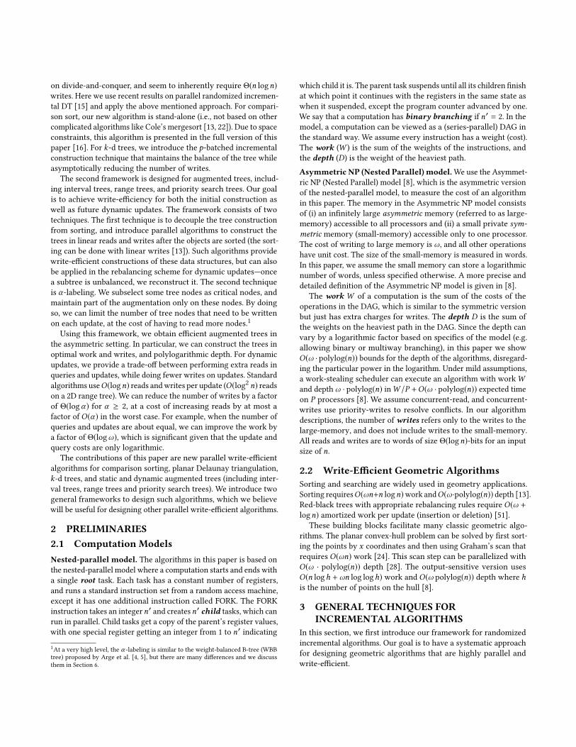
Figure 1: An example of the tracing structure. Here a pointvis added and the encroaching region contains triangles E andF (subfigure (a)). Four new triangles will be generated andreplace the two previous triangles. They may or may not becreated in the same round, and in this example this is donein two substeps (subfigures (b) and (c)). Part of the tracingstructure is shown in subfigure (d). Four neighbor trianglesA, B,C, and D are copied, and four new triangles are created.An arrow indicates that a point is encroached by the headtriangle only if it is encroached by the tail triangle.
A Linear-Write Version.We now discuss a write-efficient version
of the BGSS algorithm.We use the DAG tracing and prefix-doubling
techniques introduced in Section 3. The algorithm first computes
the DT of then/log2n earliest points in the randomized order, using
the non-write-efficient version. This step requires linear writes. It
then runs O(log logn) incremental rounds and in each round adds
a number of points equal to the number of points already inserted.
To insert points, we need to construct a search structure in the
DAG tracing problem. We can modify the BGSS algorithm to build
such a structure. In fact, the structure is effectively a subset of
the edges of the dependence graph GT (V ). In particular, in the
algorithm the only inCircle test is on Line 15. In this test, to
determine if a point encroaches t ′, we need only check its two
ancestors t and to (we need not also check the two other triangles
neighboring t , as needed inGT (V )). This leads to a DAG with depth
at most as large asGT (V ), and for which every vertex has in-degree
2. The out-degree is not necessarily constant. However, by noting
that there can be at most a constant number of outgoing edges to
each level of the DAG, we can easily transform it to a DAG with
constant out-degree by creating a copy of a triangle at each level
after it has out-neighbors. This does not increase the depth, and the
number of copies is at most proportional to the number of initial
triangles (O(n) in expectation) since the in-degrees are constant.
We refer to this as the tracing structure. An example of this structure
is shown in Figure 1.
The tracing structure can be used in the DAG tracing problem
(Definition 3.1) using the predicate f (v, t) = inCircle(v, t). Thispredicate has the traceable property since a point can only be added
to a triangle t ′ (i.e., encroaches on the triangle) if it encroached
one of the two input edges from t and to . We can therefore use the
DAG tracing algorithm to find all of the triangles encroached on
by a given point v starting at the initial root triangle tb .We first construct the DT of the first n/log
2n points in the initial
round using Algorithm 1 while building the tracing structure. Then
at the beginning of each incremental round, each point traces down
the structure to find its encroached triangles, and leaves itself in
the encroached set of that triangle. Note that the encroached set
for a given point might be large, but the average size across points
is constant in expectation.
We now analyze the cost of finding all the encroached triangles
when adding a set of new points. As discussed, the depth of Gis upper bounded by O(logn) whp. The number of encroached
triangles of a point x can be analyzed by considering the degree
of the point (number of incident triangles) if added to the DT. By
Euler’s formula, the average degree of a node in a planar graph is
at most 6. Since we add the points in a random order, the expected
value of |S(G,x)| in Theorem 3.3 is constant. Finally, the number
of all encroached (including non-leaf) triangles of this point is
upper bounded by the number of inCircle tests. Then |R(G,x)|, theexpected number of visible vertices of x , is O(logn) (Theorem 4.2
in [15]).
After finding the encroached triangles for each point being added,
we need to collect them together to add them to the triangle. This
step can be done in parallel with a semisort, which takes linear
expected work (writes) andO(ω ·polylog(m)) depthwhp [30], wherem is the number of inserted points in this round. Combining these
results leads to the following lemma.
Lemma 4.1. Given 2m points in the plane and a tracing structureTgenerated by Algorithm 1 on a randomly selected subset ofm points,computing for each triangle in T the points that encroach it amongthe remainingm points takes O(m logm + ωm) work (O(m) writes)and O(ω · polylog(m)) depth whp in the Asymmetric NP model.
The idea of the algorithm is to keep doubling the size of the set
that we add (i.e., prefix doubling). Each round applies Algorithm 1
to insert the points and build a tracing structure, and then the DAG
tracing algorithm to locate the points for the next round. The depth
of each round is upper bounded by the overall depth of the DAG on
all points, which is O(logn) whp, where n is the original size. We
obtain the following theorem.
Theorem 4.2. Planar Delaunay triangulation can be computedusing O(n logn + ωn) work (i.e., O(n) writes) in expectation andO(ω · polylog(n)) depth whp on the Asymmetric NP model withpriority-writes.
Proof. The original Algorithm 1 in [15] has O(ω · polylog(n))depthwhp. In the prefix-doubling approach, the depth of each roundis nomore thanO(ω ·polylog(n)), and the algorithm hasO(log logn)rounds. The overall depth is hence O(ω · polylog(n)) depth whp.
The work bound consists of the costs from the initial round,
and the incremental rounds. The initial round computes the trian-
gulation of the first n/log2n points, using at most O(n) inCircle
tests, O(n) writes and O(ωn) work. For the incremental rounds, we
have two components, one for locating encroached triangles in the
tracing structure, and one for applying Algorithm 1 on those points
to build the next tracing structure. The first part is handled by
Lemma 4.1. For the second part we we can apply a similar analysis
to Theorem 4.2 of [15]. In particular, the probability that there is a
dependence from a triangle in the i’th point (in the random order)
to a triangle added by a later point at location j in the ordering is
upper bounded by 24/i . Summing across all points in the second
half (we have already resolved the first half) gives:
E[C] ≤2m∑
i=m+1
2m∑j=i+1
24/i = O(m) .
This is a bound on both the number of reads and the number of
writes. Since the points added in each round doubles, the cost is
dominated by the last round, which is O(n logn) reads and O(n)writes, both in expectation. Combined with the cost of the initial
round gives the stated bounds.
5 SPACE-PARTITIONING DATASTRUCTURES
Space partitioning divides a space into non-overlapping regions.3
This process is usually applied repeatedly until the number of ob-
jects in a region is small enough, so that we can afford to answer a
query in linear work within the region. We refer to the tree struc-
ture used to represent the partitioning as the space-partitioning
tree. Commonly-used space-partitioning trees include binary space
partitioning trees, quad/oct-trees, k-d trees, and their variants, and
are widely used in computational geometry [24, 33], computer
graphics [3], integrated circuit design, learning theory, etc.
In this section, we propose write-efficient construction and up-
date algorithms for k-d trees [9]. We discuss how to support dy-
namic updates write-efficiently in Section 5.2, and we discuss how
to apply our technique to other space-partitioning trees in the full
version of this paper [16].
5.1 k-d Tree Construction and Queriesk-d trees have many variants that facilitate different queries. We
start with the most standard applications on range queries and
nearest neighbor queries, and discussions for other queries are in
the full version of this paper. A range query can be answered in
O(n(k−1)/k ) worst-case work, and an approximate (1 + ϵ)-nearest
neighbor (ANN) query requires logn · O(1/ϵ)k work assuming
bounded aspect ratio,4both in k-dimensional space. The tree to
achieve these bounds can be constructed by always partitioning
by the median of all of the objects in the current region either
on the longest dimension of the region or cycling among the kdimensions. The tree has linear size and log
2n depth [24], and can
be constructed using O(n logn) reads and writes. We now discuss
how to reduce the number of writes to O(n).One solution is to apply the incremental construction by insert-
ing the objects into a k-d tree one by one. This approach requires
linear writes,O(n logn) reads and polylogarithmic depth. However,
the splitting hyperplane is no longer based on the median, but
the object with the highest priority pre-determined by a random
permutation. The expected tree depth can be c log2n for c > 1,
but to preserve the range query cost we need the tree depth to be
log2n+O(1) (see details in Lemma 5.1). Motivated by the incremen-
tal construction, we propose the following variant, called p-batchedincremental construction, which guarantees both write-efficiency
and low tree depth.
The p-batched incremental construction. The p-batched incre-
mental construction is a variant of the classic incremental con-
struction where the dependence graph is a tree. Unlike the classic
version, where the splitting hyperplane (splitter) of a tree node is
3The other type of partitioning is object partitioning that subdivides the set of objects
directly (e.g., R-tree [32, 36], bounding volume hierarchies [29, 54]).
4The largest aspect ratio of a tree node on any two dimensions is bounded by a constant,
which is satisfied by the input instances in most real-world applications.
(a) (b) (c)
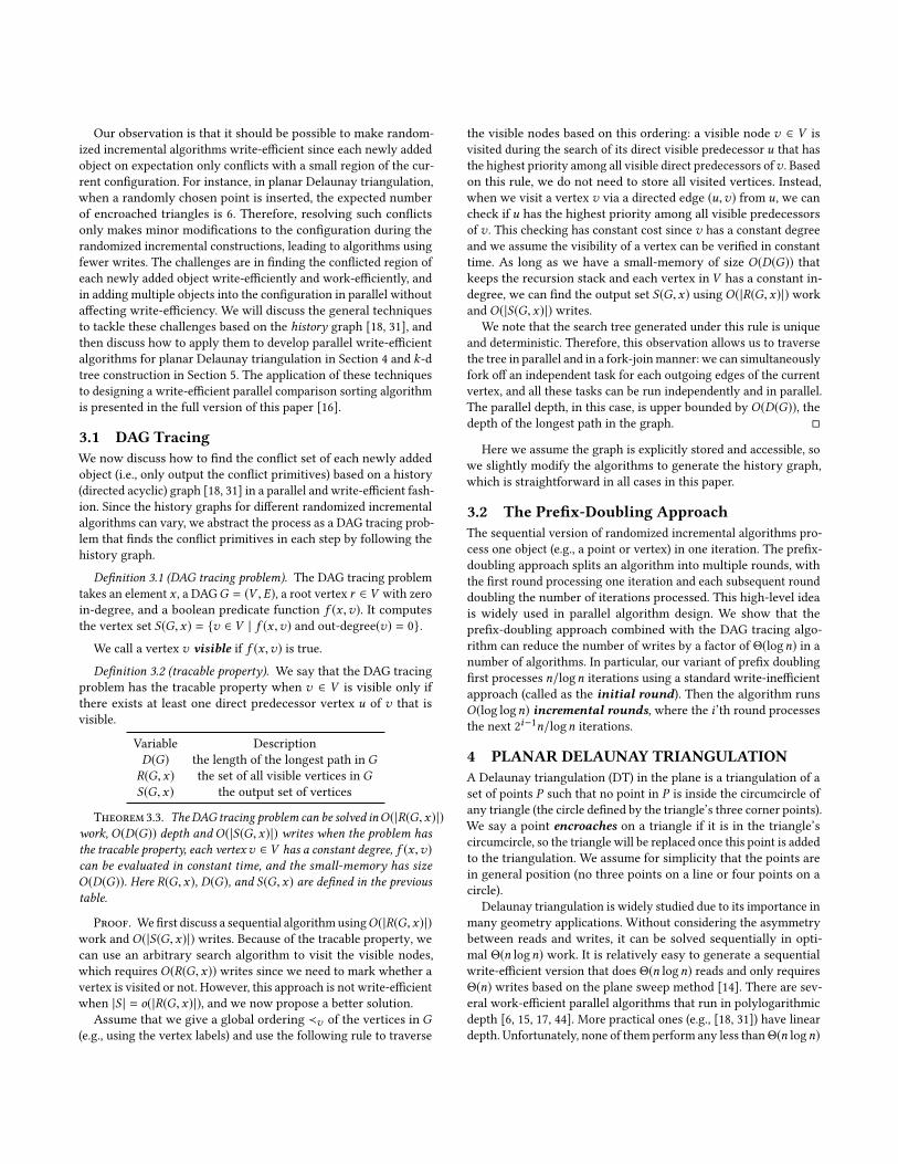
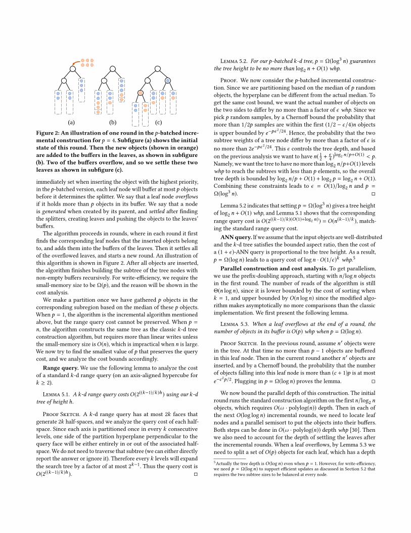
Figure 2: An illustration of one round in the p-batched incre-mental construction for p = 4. Subfigure (a) shows the initialstate of this round. Then the new objects (shown in orange)are added to the buffers in the leaves, as shown in subfigure(b). Two of the buffers overflow, and so we settle these twoleaves as shown in subfigure (c).
immediately set when inserting the object with the highest priority,
in the p-batched version, each leaf node will buffer at most p objects
before it determines the splitter. We say that a leaf node overflowsif it holds more than p objects in its buffer. We say that a node
is generated when created by its parent, and settled after finding
the splitters, creating leaves and pushing the objects to the leaves’
buffers.
The algorithm proceeds in rounds, where in each round it first
finds the corresponding leaf nodes that the inserted objects belong
to, and adds them into the buffers of the leaves. Then it settles all
of the overflowed leaves, and starts a new round. An illustration of
this algorithm is shown in Figure 2. After all objects are inserted,
the algorithm finishes building the subtree of the tree nodes with
non-empty buffers recursively. For write-efficiency, we require the
small-memory size to be Ω(p), and the reason will be shown in the
cost analysis.
We make a partition once we have gathered p objects in the
corresponding subregion based on the median of these p objects.
When p = 1, the algorithm is the incremental algorithm mentioned
above, but the range query cost cannot be preserved. When p =n, the algorithm constructs the same tree as the classic k-d tree
construction algorithm, but requires more than linear writes unless
the small-memory size isO(n), which is impractical when n is large.
We now try to find the smallest value of p that preserves the query
cost, and we analyze the cost bounds accordingly.
Range query. We use the following lemma to analyze the cost
of a standard k-d range query (on an axis-aligned hypercube for
k ≥ 2).
Lemma 5.1. A k-d range query costs O(2((k−1)/k )h ) using our k-dtree of height h.
Proof Sketch. A k-d range query has at most 2k faces that
generate 2k half-spaces, and we analyze the query cost of each half-
space. Since each axis is partitioned once in every k consecutive
levels, one side of the partition hyperplane perpendicular to the
query face will be either entirely in or out of the associated half-
space.We do not need to traverse that subtree (we can either directly
report the answer or ignore it). Therefore every k levels will expand
the search tree by a factor of at most 2k−1
. Thus the query cost is
O(2((k−1)/k )h ).
Lemma 5.2. For our p-batched k-d tree, p = Ω(log3 n) guaranteesthe tree height to be no more than log
2n +O(1) whp.
Proof. We now consider the p-batched incremental construc-
tion. Since we are partitioning based on the median of p random
objects, the hyperplane can be different from the actual median. To
get the same cost bound, we want the actual number of objects on
the two sides to differ by no more than a factor of ϵ whp. Since wepick p random samples, by a Chernoff bound the probability that
more than 1/2p samples are within the first (1/2 − ϵ/4)n objects
is upper bounded by e−pϵ2/24
. Hence, the probability that the two
subtree weights of a tree node differ by more than a factor of ϵ is
no more than 2e−pϵ2/24
. This ϵ controls the tree depth, and based
on the previous analysis we want to have n( 12+ ϵ
4)log2 n/p+O (1) < p.
Namely, wewant the tree to have nomore than log2n/p+O(1) levels
whp to reach the subtrees with less than p elements, so the overall
tree depth is bounded by log2n/p +O(1) + log
2p = log
2n +O(1).
Combining these constraints leads to ϵ = O(1)/log2n and p =
Ω(log3 n).
Lemma 5.2 indicates that settingp = Ω(log3 n) gives a tree heightof log
2n +O(1) whp, and Lemma 5.1 shows that the corresponding
range query cost is O(2((k−1)/k )(O (1)+log2 n)) = O(n(k−1)/k ), match-
ing the standard range query cost.
ANNquery. If we assume that the input objects arewell-distributed
and the k-d tree satisfies the bounded aspect ratio, then the cost of
a (1 + ϵ)-ANN query is proportional to the tree height. As a result,
p = Ω(logn) leads to a query cost of logn ·O(1/ϵ)k whp.5
Parallel construction and cost analysis. To get parallelism,
we use the prefix-doubling approach, starting with n/logn objects
in the first round. The number of reads of the algorithm is still
Θ(n logn), since it is lower bounded by the cost of sorting when
k = 1, and upper bounded by O(n logn) since the modified algo-
rithm makes asymptotically no more comparisons than the classic
implementation. We first present the following lemma.
Lemma 5.3. When a leaf overflows at the end of a round, thenumber of objects in its buffer is O(p) whp when p = Ω(logn).
Proof Sketch. In the previous round, assume n′ objects werein the tree. At that time no more than p − 1 objects are bufferedin this leaf node. Then in the current round another n′ objects areinserted, and by a Chernoff bound, the probability that the number
of objects falling into this leaf node is more than (c + 1)p is at most
e−c2p/2
. Plugging in p = Ω(logn) proves the lemma.
We now bound the parallel depth of this construction. The initial
round runs the standard construction algorithm on the firstn/log2n
objects, which requires O(ω · polylog(n)) depth. Then in each of
the next O(log logn) incremental rounds, we need to locate leaf
nodes and a parallel semisort to put the objects into their buffers.
Both steps can be done in O(ω · polylog(n)) depth whp [30]. Then
we also need to account for the depth of settling the leaves after
the incremental rounds. When a leaf overflows, by Lemma 5.3 we
need to split a set of O(p) objects for each leaf, which has a depth
5Actually the tree depth is O (logn) even when p = 1. However, for write-efficiency,
we need p = Ω(logn) to support efficient updates as discussed in Section 5.2 that
requires the two subtree sizes to be balanced at every node.

of O(ω · polylog(n)) using the classic approach, and is applied for
no more than a constant number of times whp by Lemma 5.3.
We now analyze the number of writes this algorithm requires.
The initial round requires O(n) writes as it uses a standard con-
struction algorithm on n/log2n objects. In the incremental rounds,
O(1) writes whp are required for each object to find the leaf node it
belongs to and add itself to the buffer using semisorting [30]. From
Lemma 5.3, when finding the splitting hyperplane and splitting the
object for a tree node, the number of writes required is O(p) whp.Note that after a new leaf node is generated from a split, it contains
at least p/2 objects. Therefore, after all incremental rounds, the
tree contains at most O(n/p) tree nodes, and the overall writes to
generate them is O((n/p) · p) = O(n). After the incremental rounds
finish, we need O(n) writes to settle the leaves with non-empty
buffers, assuming O(p) cache size. In total, the algorithm uses O(n)writes whp.
Theorem 5.4. A k-d tree that supports range and ANN queriesefficiently can be computed using O(n logn +ωn) expected work (i.e.,O(n) writes) andO(ω · polylog(n)) depth whp in the Asymmetric NPmodel. For range query the small-memory size required is Ω(log3 n).
5.2 k-d Tree Dynamic UpdatesUnlike many other tree structures, we cannot rotate the tree nodes
ink-d trees since each tree node represents a subspace instead of justa set of objects. Deletion is simple for k-d trees, since we can afford
to reconstruct the whole structure from scratch when a constant
fraction of the objects in the k-d tree have been removed, and
before the reconstruction we just mark the deleted node (constant
reads and writes per deletion via an unordered map). In total, the
amortized cost of each deletion is O(ω + logn). For insertions, wediscuss two techniques that optimize either the update cost or the
query cost.
Logarithmic reconstruction [41]. We maintain at most log2n
k-d trees of sizes that are increasing powers of 2. When an object is
inserted, we create a k-d tree of size 1 containing the object. While
there are trees of equal size, we flatten them and replace the two
trees with a tree of twice the size. This process keeps repeating until
there are no trees with the same size. When querying, we search in
all (at most log2n) trees. Using this approach, the number of reads
and writes on an insertion isO(log2 n), and on a deletion isO(logn).
The costs for range queries and ANN queries are O(n(k−1)/k ) and
log2 n ·O(1/ϵ)k respectively, plus the cost for writing the output.
If we apply our write-efficient p-batched version when recon-
structing the k-d trees, we can reduce the writes (but not reads) by
a factor of O(logn) (i.e., O(logn) and O(1) writes per update).When using logarithmic reconstruction, querying up toO(logn)
trees can be inefficient in some cases, so here we show an alternative
solution that only maintains a single tree.
Single-tree version. As discussed in Section 5.1, only the tree
height affects the costs for range queries and ANN queries. For
range queries, Lemma 5.2 indicates that the tree height should be
log2n +O(1) to guarantee the optimal query cost. To maintain this,
we can tolerate an imbalance between the weights of two subtrees
by a factor of O(1/logn), and reconstruct the subtree when the
imbalance is beyond the constraint. In the worst case, a subtree of
size n′ is rebuilt once after O(n′/logn) insertions into the subtree.
Since the reconstructing a subtree of size n′ requires O(n′ logn′ +ωn′)work, each inserted object contributesO(logn logn′+ω logn)work to every node on its tree path, and there are O(logn) suchnodes. Hence, the amortized work for an insertion is O(log3 n +ω log
2 n). For efficient ANN queries, we only need the tree height
to be O(logn), which can be guaranteed if the imbalance between
two subtree sizes is at most a constant multiplicative factor. Using
a similar analysis, in this case the amortized work for an insertion
is O(log2 n + ω logn).
6 AUGMENTED TREESAn augmented tree is a tree that keeps extra data on each tree
node other than what is used to maintain the balance of this tree.
We refer to the extra data on each tree node as the augmentation.In this section, we introduce a framework that gives new algo-
rithms for constructing both static and dynamic augmented trees
including interval trees, 2D range trees, and priority search trees
that are parallel and write-efficient. Using these data structures
we can answer 1D stabbing queries, 2D range queries, and 3-sided
queries (defined in Section 6.1). For all three problems, we assume
that the query results need to be written to the large-memory. Our
results are summarized in Table 1. We improve upon the traditional
algorithms in two ways. First, we show how to construct inter-
val trees and priority search trees using O(n) instead of O(n logn)writes (since the 2D range tree requiresO(n logn) storagewe cannotasymptotically reduce the number of writes). Second, we provide
a tradeoff between update costs and query costs in the dynamic
versions of the data structures. The cost bounds are parameterized
by α . By setting α = O(1) we achieve the same cost bounds as the
traditional algorithms for queries and updates. α can be chosen
optimally if we know the update-to-query ratio r . For interval andpriority trees, the optimal value of α ismin(2+ω/r ,ω). The overallwork without considering writing the output can be improved by
a factor of Θ(logα). For 2D range trees, the optimal value of α is
2 +min(ω/r ,ω)/log2n.
We discuss two techniques in this section that we use to achieve
write-efficiency. The first technique is to decouple the tree construc-
tion from sorting, and we introduce efficient algorithms to construct
interval and priority search trees in linear reads and writes after the
input is sorted. Sorting can be done in parallel and write-efficiently
(linear writes).Using this approach, the tree structure that we obtain
is perfectly balanced.
The second technique that we introduce is the α-labeling tech-nique.Wemark a subset of tree nodes as critical nodes by a predicatefunction parameterized by α , and only maintain augmentations
on these critical nodes. We can then guarantee that every update
only modifies O(logα n) nodes, instead of O(logn) nodes as in the
classic algorithms. At a high level, the α-labeling is similar to the
weight-balanced B-tree (WBB tree) proposed by Arge et al. [4, 5]
for the external-memory (EM) model [1]. However, as we discuss
in Section 6.3, directly applying the EM algorithms [2, 4, 5, 47, 48]
does not give us the desired bounds in our model. Secondly, our
underlying tree is still binary. Hence, we mostly need no changes to
the algorithmic part that dynamically maintains the augmentation
in this trees, but just relax the balancing criteria so the underlying
search trees can be less balanced. An extra benefit of our framework
Construction Query Update
Classic interval tree O(ωn logn) O(ωk + logn) O(ω logn)
Our interval tree O(ωn + n logn) O(ωk + α logα n) O((ω + α) logα n)
Classic priority search tree O(ωn logn) O(ωk + logn) O(ω logn)
Our priority search tree O(ωn + n logn) O(ωk + α logα n) O((ω + α) logα n)
Classic range Tree O(ωn logn) O(ωk + log2 n) O((logn + ω) logn)
Our range tree O((α + ω)n logα n) O(ωk + α logα n logn) O((α logn + ω) logα n)
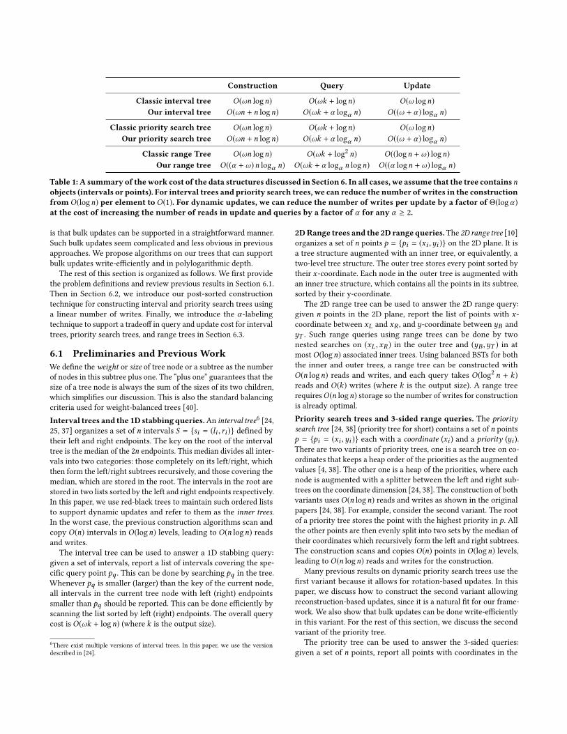
Table 1: A summary of thework cost of the data structures discussed in Section 6. In all cases, we assume that the tree containsnobjects (intervals or points). For interval trees and priority search trees, we can reduce the number ofwrites in the constructionfrom O(logn) per element to O(1). For dynamic updates, we can reduce the number of writes per update by a factor of Θ(logα)at the cost of increasing the number of reads in update and queries by a factor of α for any α ≥ 2.
is that bulk updates can be supported in a straightforward manner.
Such bulk updates seem complicated and less obvious in previous
approaches. We propose algorithms on our trees that can support
bulk updates write-efficiently and in polylogarithmic depth.
The rest of this section is organized as follows. We first provide
the problem definitions and review previous results in Section 6.1.
Then in Section 6.2, we introduce our post-sorted construction
technique for constructing interval and priority search trees using
a linear number of writes. Finally, we introduce the α-labelingtechnique to support a tradeoff in query and update cost for interval
trees, priority search trees, and range trees in Section 6.3.
6.1 Preliminaries and Previous WorkWe define the weight or size of tree node or a subtree as the number
of nodes in this subtree plus one. The “plus one” guarantees that the
size of a tree node is always the sum of the sizes of its two children,
which simplifies our discussion. This is also the standard balancing
criteria used for weight-balanced trees [40].
Interval trees and the 1D stabbing queries.An interval tree6 [24,25, 37] organizes a set of n intervals S = si = (li , ri ) defined by
their left and right endpoints. The key on the root of the interval
tree is the median of the 2n endpoints. This median divides all inter-
vals into two categories: those completely on its left/right, which
then form the left/right subtrees recursively, and those covering the
median, which are stored in the root. The intervals in the root are
stored in two lists sorted by the left and right endpoints respectively.
In this paper, we use red-black trees to maintain such ordered lists
to support dynamic updates and refer to them as the inner trees.In the worst case, the previous construction algorithms scan and
copy O(n) intervals in O(logn) levels, leading to O(n logn) readsand writes.
The interval tree can be used to answer a 1D stabbing query:
given a set of intervals, report a list of intervals covering the spe-
cific query point pq . This can be done by searching pq in the tree.
Whenever pq is smaller (larger) than the key of the current node,
all intervals in the current tree node with left (right) endpoints
smaller than pq should be reported. This can be done efficiently by
scanning the list sorted by left (right) endpoints. The overall query
cost is O(ωk + logn) (where k is the output size).
6There exist multiple versions of interval trees. In this paper, we use the version
described in [24].
2DRange trees and the 2D range queries.The 2D range tree [10]organizes a set of n points p = pi = (xi ,yi ) on the 2D plane. It is
a tree structure augmented with an inner tree, or equivalently, a
two-level tree structure. The outer tree stores every point sorted by
their x-coordinate. Each node in the outer tree is augmented with
an inner tree structure, which contains all the points in its subtree,
sorted by their y-coordinate.
The 2D range tree can be used to answer the 2D range query:
given n points in the 2D plane, report the list of points with x-coordinate between xL and xR , and y-coordinate between yB and
yT . Such range queries using range trees can be done by two
nested searches on (xL ,xR ) in the outer tree and (yB ,yT ) in at
most O(logn) associated inner trees. Using balanced BSTs for both
the inner and outer trees, a range tree can be constructed with
O(n logn) reads and writes, and each query takes O(log2 n + k)reads and O(k) writes (where k is the output size). A range tree
requiresO(n logn) storage so the number of writes for construction
is already optimal.
Priority search trees and 3-sided range queries. The prioritysearch tree [24, 38] (priority tree for short) contains a set of n points
p = pi = (xi ,yi ) each with a coordinate (xi ) and a priority (yi ).There are two variants of priority trees, one is a search tree on co-
ordinates that keeps a heap order of the priorities as the augmented
values [4, 38]. The other one is a heap of the priorities, where each
node is augmented with a splitter between the left and right sub-
trees on the coordinate dimension [24, 38]. The construction of both
variants uses O(n logn) reads and writes as shown in the original
papers [24, 38]. For example, consider the second variant. The root
of a priority tree stores the point with the highest priority in p. Allthe other points are then evenly split into two sets by the median of
their coordinates which recursively form the left and right subtrees.
The construction scans and copies O(n) points in O(logn) levels,leading to O(n logn) reads and writes for the construction.
Many previous results on dynamic priority search trees use the
first variant because it allows for rotation-based updates. In this
paper, we discuss how to construct the second variant allowing
reconstruction-based updates, since it is a natural fit for our frame-
work. We also show that bulk updates can be done write-efficiently
in this variant. For the rest of this section, we discuss the second
variant of the priority tree.
The priority tree can be used to answer the 3-sided queries:
given a set of n points, report all points with coordinates in the
range [xL ,xR ], and priority higher than yB . This can be done by
traversing the tree, skipping the subtrees whose coordinate range
do not overlap [xL ,xR ], or where the priority in the root is lower
than yB . The cost of each query is O(ωk + logn) for an output of
size k [24].
6.2 The Post-Sorted ConstructionFor interval trees and priority search trees, the standard construc-
tion algorithms [23–25, 37, 38] require O(n logn) reads and writes,
even though the output is only of linear size. This section describes
algorithms for constructing them in an optimal linear number of
writes. Both algorithms first sort the input elements by their x-coordinate in O(ωn + n logn) work and O(ω · polylog(n)) depthusing the write-efficient comparison sort described in the full ver-
sion of this paper [16]. We now describe how to build the trees
in O(n) reads and writes given the sorted input. For a range tree,
since the standard tree has O(n logn) size, the classic constructionalgorithm is already optimal.
Interval Tree. After we sort all 2n coordinates of the endpoints,
we can first build a perfectly-balanced binary search tree on the
endpoints usingO(n) reads and writes andO(ω · polylog(n)) depth.We now consider how to construct the inner tree of each tree node.
We create a lowest common ancestor (LCA) data structure on
the keys of the tree nodes that allows for constant time queries.
This can be constructed in O(n) reads/writes and O(ω · polylog(n))depth [11, 35]. Each interval can then find the tree node that it
belongs to using an LCA query on its two endpoints. We then use
a radix sort on the n intervals. The key of an interval is a pair with
the first value being the index of the tree node that the interval
belongs to, and the second value being the index of the left endpoint
in the pre-sorted order. The sorted result gives the interval list for
each tree node sorted by left endpoints. We do the same for the
right endpoints. This step takes O(n) reads/writes overall. Finally,we can construct the inner trees from the sorted intervals in O(n)reads/writes across all tree nodes.
Parallelism is straightforward for all steps except for the radix
sort. The number of possible keys can beO(n2), and it is not knownhow to radix sort keys from such a range work-efficiently and in
polylogarithmic depth. However, we can sort a range of O(n logn)in O(ωn) expected work and O(ω · polylog(n)) depth whp [43].
Hence our goal is to limit the first value into a O(logn) range. We
note that given the left endpoint of an interval, there are only
log2(2n) possible locations for the tree node (on the tree path) of
this interval. Therefore instead of using the tree node as the first
value of the key, we use the level of the tree node, which is in the
range [1, . . . ,O(logn)]. By radix sorting these pairs, so we have thesorted intervals (based on left or right endpoint) for each level. We
observe that the intervals of each tree node are consecutive in the
sorted interval list per level. This is because for tree nodes u1 andu2 on the same level where u1 is to the left of u2, the endpoints ofu1’s intervals must all be to the left of u2’s intervals. Therefore, inparallel we can find the first and the last intervals of each node
in the sorted list, and construct the inner tree of each node. Since
the intervals are already sorted based on the endpoints, we can
build inner trees in O(n) reads and writes and O(ω · polylog(n))depth [12].
Priority Tree. In the original priority tree construction algorithm,
points are recursively split into sub-problems based on the median
at each node of the tree. This requires O(n) writes at each level
of the tree if we explicitly copy the nodes and pack out the root
node that is removed. To avoid explicit copying, since the points
are already pre-sorted, our write-efficient construction algorithm
passes indices determining the range of points belonging to a sub-
problem instead of actually passing the points themselves. To avoid
packing, we simply mark the position of the removed point in the
list as invalid, leaving a hole, and keep track of the number of valid
points in each sub-problem.
Our recursive construction algorithm works as follows. For a
tree node, we know the range of the points it represents, as well
as the number of valid points nv . We then pick the valid point
with the highest priority as the root, mark the point as invalid,
find the median among the valid points, and pass the ranges based
on the median and number of valid points (either ⌊(nv − 1)/2⌋ or⌈(nv − 1)/2⌉) to the left and right sub-trees, which are recursively
constructed. The base case is when there is only one valid point
remaining, or when the number of holes is more than the valid
points. Since each node in the tree can only cause one hole, for every
range corresponding to a node, there are at most O(logn) holes.Since the size of the small-memory is Ω(logn), when the number
of valid points is fewer than the number of holes, we can simply
load all of the valid points into the small-memory and construct
the sub-tree.
To efficiently implement this algorithm, we need to support three
queries on the input list: finding the root, finding the k-th element
in a range (e.g., the median), and deleting an element. All queries
and updates can be supported using a standard tournament tree
where each interior node maintains the minimum element and the
number of valid nodes within the subtree. With a careful analysis,
all queries and updates throughout the construction require linear
reads/writes overall. The details are provided in the full version of
this paper [16].
The parallel depth is O(ω · polylog(n))—the bottleneck lies in
removing the points. There are O(logn) levels in the priority tree
and it costsO(ω logn) for removing elements from the tournament
tree on each level. For the base cases, it takes linear writes overall to
load the points into the small-memory and linear writes to generate
all tree nodes. The depth is O(ω logn).We summarize our result in this section in Theorem 6.1.
Theorem 6.1. An interval tree or a priority search tree can beconstructed with pre-sorted input in O(ωn) expected work and O(ω ·polylog(n)) depth whp on the Asymmetric NP model.
6.3 Dynamic Updates usingReconstruction-Based Rebalancing
Dynamic updates (insertions and deletions) are often supported
on augmented trees [23–25, 37, 38] and the goal of this section
is to support updates write-efficiently, at the cost of performing
extra reads to reduce the overall work. Traditionally, an insertion or
deletion costs O(logn) for interval trees and priority search trees,
and O(log2 n) for range trees. In the asymmetric setting, the work
is multiplied by ω. To reduce the overall work, we introduce an
approach to select a subset of tree nodes as critical nodes, and only
update the balance information of those nodes (the augmentations
are mostly unaffected). The selection of these critical nodes are done
by the α-labeling introduced in Section 6.3.1. Roughly speaking, for
each tree path from the root to a leaf node, we haveO(logα n) criti-cal nodes marked such that the subtree weights of two consecutive
marked nodes differ by about a factor of α ≥ 2. By doing so, we
only need to update the balancing information in the critical nodes,
leading to fewer tree nodes modified in an update.
Arge et al. [4, 5] use a similar strategy to support dynamic up-
dates on augmented trees in the external-memory (EM) model, in
which a block of data can be transferred in unit cost [1]. They use
a B-tree instead of a binary tree, which leads to a shallower tree
structure and fewer memory accesses in the EMmodel. However, in
the Asymmetric NP model, modifying a block of data requires work
proportional to the block size, and directly using their approach
cannot reduce the overall work. Inspired by their approach, we
propose a simple approach to reduce the work of updates for the
Asymmetric NP model.
The main component of our approach is reconstruction-basedrebalancing using the α-labeling technique. We can always obtain
the sorted order via the tree structure, so when imbalance occurs,
we can afford to reconstruct the whole subtree in reads and writes
proportional to the subtree size and polylogarithmic depth. This
gives a unified approach for different augmented trees: interval
trees, priority search trees, and range trees.
We introduce the α-labeling idea in Section 6.3.1, the rebalancingalgorithm in Section 6.3.2, and its work analysis in Section 6.3.3.
We then discuss the maintenance of augmented values for different
applications in Section 6.3.4. We mention how to parallelize bulk
updates in Section 6.3.5 and in the full version of the paper [16].
6.3.1 α-Labeling. The goal of the α-labeling is to maintain the
balancing information at only a subset of tree nodes, the critical
nodes, such that the number of writes per update is reduced. Once
the augmented tree is constructed, we label the node as a critical
node if for some integer i ≥ 0, (1) its subtree weight is between 2α i
and 4α i − 2 (inclusive); or (2) its subtree weight is 2α i − 1 and its
sibling’s subtree weight is 2α i . All other nodes are secondary nodes.
As a special case, we always treat the root as a virtual critical
node, but it does not necessary satisfy the invariants of critical
nodes. Note that all leaf nodes are critical nodes in α-labeling sincethey always have subtrees of weight 2. When we label a critical
node, we refer to its current subtree weight (which may change
after insertions/deletions) as its initial weight. Note that after theaugmented tree is constructed, we can find and mark the critical
nodes in O(n) reads/writes and O(ω logn) depth. After that, weonly maintain the subtree weights for these critical nodes, and use
their weights to balance the tree.
Fact 6.2. For a critical node A, 2α i − 1 ≤ |A| ≤ 4α i − 2 holds forsome integer i .
This fact directly follows the definition of the critical node.
For two critical nodes A and B, if A is B’s ancestor and there is
no other critical node on the tree path between them, we refer to Bas A’s critical child, and A as B’s critical parent. We define a criticalsibling accordingly.
We show the following lemma on the initial weights.
Lemma 6.3. For any two critical nodes A and B where A is B’scritical parent, their initial weights satisfymax(α/2)|B |, 2|B | − 1 ≤|A| ≤ (2α + 1)|B |.
Proof. Based on Fact 6.2, we assume 2α i −1 ≤ |A| ≤ 4α i −2 and2α j −1 ≤ |B | ≤ 4α j −2 for some integers i and j . We first show that
i = j + 1. It is easy to check that j cannot be larger than or equal to
i . Assume by contradiction that j < i − 1. With this assumption, we
will show that there exists an ancestor of B, which we refer to it asy,which is a critical node. The existence of y contradicts the fact that
A is B’s critical parent. We will use the property that for any tree
node x the weight of its parent p(x) is 2|x | − 1 ≤ |p(x)| ≤ 2|x | + 1.Assume that B does not have such an ancestor y. Let z be the
ancestor of B with weight closest to but no more than 2α i−1. We
consider two cases: (a) |z | ≤ 2α i−1 − 2 and (b) |z | = 2α i−1 − 1. Incase (a) z’s parent p(z) has weight at most 2|z |+1 = 4α i−1−3. |p(z)|cannot be less than 2α i−1 by definition of z, and soy = p(z), leadingto a contradiction. In case (b), z’s sibling does not have weight 2α i−1,otherwisey = z. However, then |p(z)| ≤ 2|z | = 4α i−1−2, and eitherz is not the ancestor with weight closest to 2α i−1 or y = p(z).
Given i = j + 1, we have (α/2)|B | ≤ |A| ≤ (2α + 1)|B | (byplugging in 2α i − 1 ≤ |A| ≤ 4α i − 2 and 2α i−1 − 1 ≤ |B | ≤ 4α i−1 −2). Furthermore, since A is B’s ancestor, we have 2|B | − 1 ≤ |A|.Combining the results proves the lemma.
6.3.2 Rebalancing Algorithm based on α -Labeling. We now con-
sider insertions and deletions on an augmented tree. Maintaining
the augmented values on the tree are independent of our α-labelingtechnique, and differs slightly for each of the three tree structures.
We will further discuss how to maintain augmented values in Sec-
tion 6.3.4.
We note that deletions can be handled by marking the deleted
objects without actually applying the deletion, and reconstructing
the whole subtree once a constant fraction of the objects is deleted.
Therefore in this section, we first focus on the insertions only. We
analyze single insertions here, and discuss bulk insertions in the
full version of the paper [16]. Once the subtree weight of a critical
node A reaches twice the initial weight s , we reconstruct the wholesubtree, label the critical nodes within the subtree, and recalculate
the initial weights of the new critical nodes. An exception here is
that, if s ≤ 4α i − 2 and 2α i+1 − 1 ≤ 2s for a certain i , we do not
mark the new root since otherwise it violates the bound stated in
Lemma 6.4 (see more details in Section 6.3.3) withA’s critical parent.After this reconstruction, A’s original critical parent gets one extracritical child, and the two affected children now have initial weights
the same asA’s initial weight. If imbalance occurs at multiple levels,
we reconstruct the topmost tree node. An illustration of this process
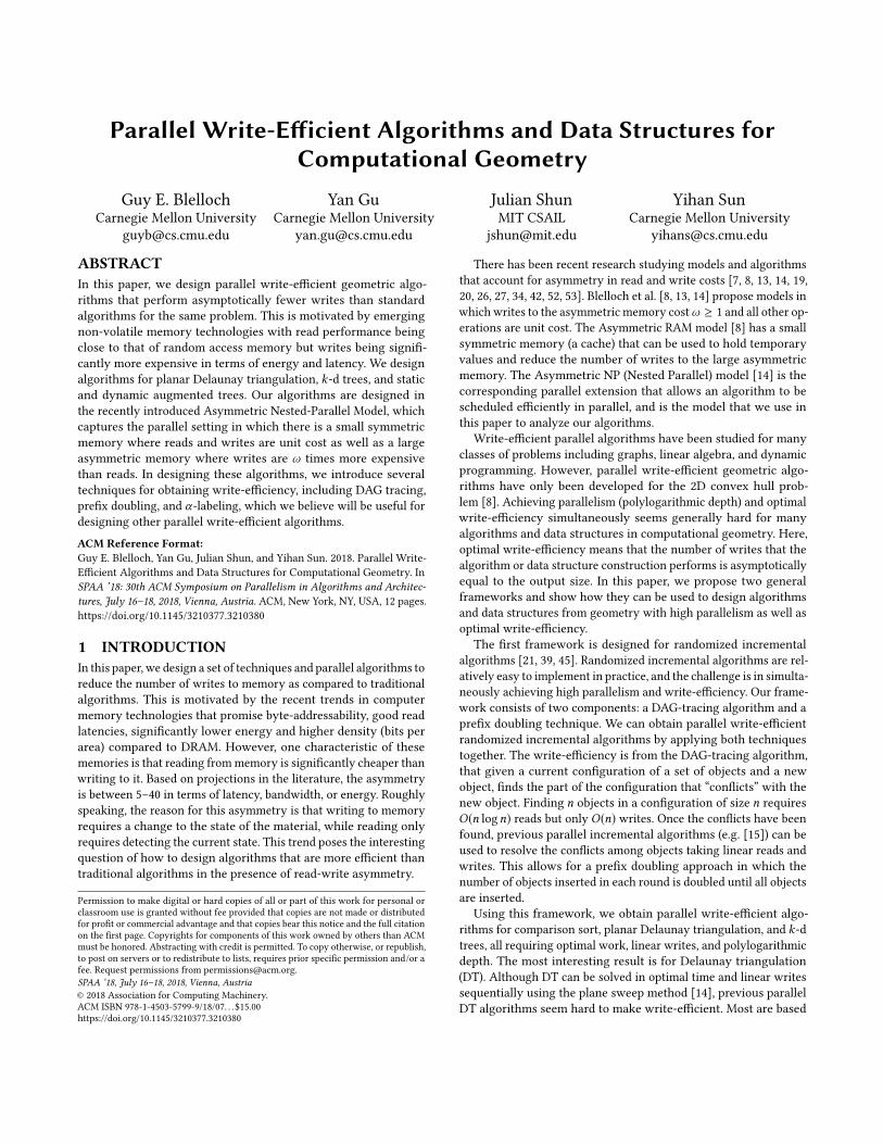
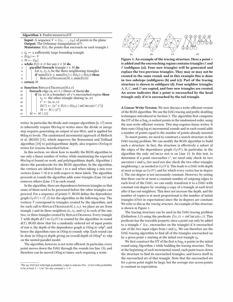
is shown in Figure 3.
We can directly apply the algorithms in Section 6.2 to reconstruct
a subtree as long as we have the sorted order of the (end)points
in this subtree. For interval and range trees, we can acquire the
sorted order by traversing the subtree. using linear work andO(ω ·polylog(n)) depth [8, 46]. For priority trees, since the tree nodes are
not stored in-order, we need to insert all interior nodes into the tree
in a bottom-up order based on their coordinates (without applying
rebalancing) to get the total order on coordinates of all points (the
details and cost analysis can be found in the full version of this
(a) (b) (c)
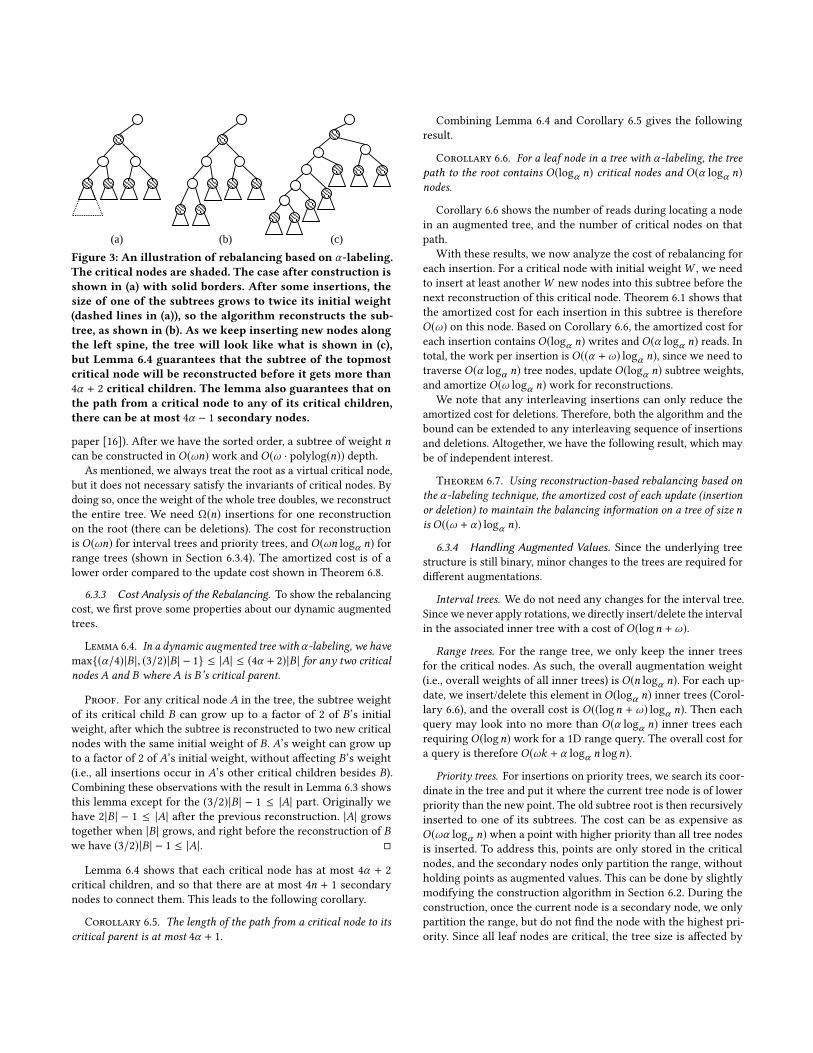
Figure 3: An illustration of rebalancing based on α-labeling.The critical nodes are shaded. The case after construction isshown in (a) with solid borders. After some insertions, thesize of one of the subtrees grows to twice its initial weight(dashed lines in (a)), so the algorithm reconstructs the sub-tree, as shown in (b). As we keep inserting new nodes alongthe left spine, the tree will look like what is shown in (c),but Lemma 6.4 guarantees that the subtree of the topmostcritical node will be reconstructed before it gets more than4α + 2 critical children. The lemma also guarantees that onthe path from a critical node to any of its critical children,there can be at most 4α − 1 secondary nodes.
paper [16]). After we have the sorted order, a subtree of weight ncan be constructed in O(ωn) work and O(ω · polylog(n)) depth.
As mentioned, we always treat the root as a virtual critical node,
but it does not necessary satisfy the invariants of critical nodes. By
doing so, once the weight of the whole tree doubles, we reconstruct
the entire tree. We need Ω(n) insertions for one reconstruction
on the root (there can be deletions). The cost for reconstruction
is O(ωn) for interval trees and priority trees, and O(ωn logα n) forrange trees (shown in Section 6.3.4). The amortized cost is of a
lower order compared to the update cost shown in Theorem 6.8.
6.3.3 Cost Analysis of the Rebalancing. To show the rebalancing
cost, we first prove some properties about our dynamic augmented
trees.
Lemma 6.4. In a dynamic augmented tree with α -labeling, we havemax(α/4)|B |, (3/2)|B | − 1 ≤ |A| ≤ (4α + 2)|B | for any two criticalnodes A and B where A is B’s critical parent.
Proof. For any critical node A in the tree, the subtree weight
of its critical child B can grow up to a factor of 2 of B’s initialweight, after which the subtree is reconstructed to two new critical
nodes with the same initial weight of B. A’s weight can grow up
to a factor of 2 of A’s initial weight, without affecting B’s weight(i.e., all insertions occur in A’s other critical children besides B).Combining these observations with the result in Lemma 6.3 shows
this lemma except for the (3/2)|B | − 1 ≤ |A| part. Originally we
have 2|B | − 1 ≤ |A| after the previous reconstruction. |A| growstogether when |B | grows, and right before the reconstruction of Bwe have (3/2)|B | − 1 ≤ |A|.
Lemma 6.4 shows that each critical node has at most 4α + 2
critical children, and so that there are at most 4n + 1 secondary
nodes to connect them. This leads to the following corollary.
Corollary 6.5. The length of the path from a critical node to itscritical parent is at most 4α + 1.
Combining Lemma 6.4 and Corollary 6.5 gives the following
result.
Corollary 6.6. For a leaf node in a tree with α -labeling, the treepath to the root contains O(logα n) critical nodes and O(α logα n)nodes.
Corollary 6.6 shows the number of reads during locating a node
in an augmented tree, and the number of critical nodes on that
path.
With these results, we now analyze the cost of rebalancing for
each insertion. For a critical node with initial weightW , we need
to insert at least anotherW new nodes into this subtree before the
next reconstruction of this critical node. Theorem 6.1 shows that
the amortized cost for each insertion in this subtree is therefore
O(ω) on this node. Based on Corollary 6.6, the amortized cost for
each insertion contains O(logα n) writes and O(α logα n) reads. Intotal, the work per insertion is O((α + ω) logα n), since we need to
traverse O(α logα n) tree nodes, update O(logα n) subtree weights,and amortize O(ω logα n) work for reconstructions.
We note that any interleaving insertions can only reduce the
amortized cost for deletions. Therefore, both the algorithm and the
bound can be extended to any interleaving sequence of insertions
and deletions. Altogether, we have the following result, which may
be of independent interest.
Theorem 6.7. Using reconstruction-based rebalancing based onthe α -labeling technique, the amortized cost of each update (insertionor deletion) to maintain the balancing information on a tree of size nis O((ω + α) logα n).
6.3.4 Handling Augmented Values. Since the underlying tree
structure is still binary, minor changes to the trees are required for
different augmentations.
Interval trees. We do not need any changes for the interval tree.
Since we never apply rotations, we directly insert/delete the interval
in the associated inner tree with a cost of O(logn + ω).
Range trees. For the range tree, we only keep the inner trees
for the critical nodes. As such, the overall augmentation weight
(i.e., overall weights of all inner trees) is O(n logα n). For each up-
date, we insert/delete this element in O(logα n) inner trees (Corol-lary 6.6), and the overall cost is O((logn + ω) logα n). Then each
query may look into no more than O(α logα n) inner trees eachrequiring O(logn) work for a 1D range query. The overall cost for
a query is therefore O(ωk + α logα n logn).
Priority trees. For insertions on priority trees, we search its coor-
dinate in the tree and put it where the current tree node is of lower
priority than the new point. The old subtree root is then recursively
inserted to one of its subtrees. The cost can be as expensive as
O(ωα logα n) when a point with higher priority than all tree nodes
is inserted. To address this, points are only stored in the critical
nodes, and the secondary nodes only partition the range, without
holding points as augmented values. This can be done by slightly
modifying the construction algorithm in Section 6.2. During the
construction, once the current node is a secondary node, we only
partition the range, but do not find the node with the highest pri-
ority. Since all leaf nodes are critical, the tree size is affected by
at most a factor of 2. With this approach, each insertion modifies
at most O(logα n) nodes, and so the extra work per insertion for
maintaining augmented data is O((α + ω) logα n). A deletion on
priority trees can be implemented symmetrically, and can lead to
cascading promotions of the points. Once the promotions occur,
we leave a dummy node in the original place of the last promoted
point, so that all of the subtree sizes remain unchanged (and the
tree is reconstructed once half one the nodes are dummy). The cost
of a deletion is also O((α + ω) logα n).Combining the results above gives the following theorem.
Theorem 6.8. Given any integer α ≥ 2, an update on an intervalor priority search tree requires O((ω + α) logα n) amortized workand a query costs O(ωk + α logα n); for a 2D range tree, the queryand amortized update cost is O((α logn + ω) logα n) and O(ωk +α logα n logn).
6.3.5 Bulk Updates. One of the benefits of the reconstruction-based approach is that bulk updates on our augmented trees can
be directly supported. In this case we need to change the inner
trees to be treaps to support efficient bulk insertions/deletions [12,
49, 50]. We discuss the details bulk updates in the full version of
this paper [16]. The overall conclusion is that, given a bulk update
of sizem, we can process it in parallel using the same amount of
work as applying the updates sequentially, and inO(ω · polylog(n))depth.
ACKNOWLEDGMENTSThis work was supported in part by NSF grants CCF-1408940, CCF-
1533858, and CCF-1629444.
REFERENCES[1] A. Aggarwal and J. S. Vitter. The Input/Output complexity of sorting and related
problems. Communications of the ACM, 31(9), 1988.
[2] D. Ajwani, N. Sitchinava, and N. Zeh. Geometric algorithms for private-cache
chip multiprocessors. In ESA, 2010.[3] T. Akenine-Möller, E. Haines, and N. Hoffman. Real-time rendering. CRC Press,
2008.
[4] L. Arge, V. Samoladas, and J. S. Vitter. On two-dimensional indexability and
optimal range search indexing. In PODS, 1999.[5] L. Arge and J. S. Vitter. Optimal external memory interval management. SIAM
Journal on Computing, 32(6), 2003.[6] M. Atallah and M. Goodrich. Deterministic parallel computational geometry. In
Synthesis of Parallel Algorithms, pages 497–536. Morgan Kaufmann, 1993.
[7] A. Ben-Aroya and S. Toledo. Competitive analysis of flash-memory algorithms.
In ESA, 2006.[8] N. Ben-David, G. E. Blelloch, J. T. Fineman, P. B. Gibbons, Y. Gu, C. McGuffey,
and J. Shun. Parallel algorithms for asymmetric read-write costs. In SPAA, 2016.[9] J. L. Bentley. Multidimensional binary search trees used for associative searching.
Communications of the ACM, 18(9), 1975.
[10] J. L. Bentley. Decomposable searching problems. Information Processing Letters,8(5), 1979.
[11] O. Berkman and U. Vishkin. Recursive *-tree parallel data-structure. In FOCS,1989.
[12] G. E. Blelloch, D. Ferizovic, and Y. Sun. Just join for parallel ordered sets. In
SPAA, 2016.[13] G. E. Blelloch, J. T. Fineman, P. B. Gibbons, Y. Gu, and J. Shun. Sorting with
asymmetric read and write costs. In SPAA, 2015.[14] G. E. Blelloch, J. T. Fineman, P. B. Gibbons, Y. Gu, and J. Shun. Efficient algorithms
with asymmetric read and write costs. In ESA, 2016.[15] G. E. Blelloch, Y. Gu, J. Shun, and Y. Sun. Parallelism in randomized incremental
algorithms. In SPAA, 2016.[16] G. E. Blelloch, Y. Gu, J. Shun, and Y. Sun. Parallel write-efficient algorithms and
data structures for computational geometry. arXiv preprint:1805.05592, 2018.
[17] G. E. Blelloch, J. C. Hardwick, G. L. Miller, and D. Talmor. Design and imple-
mentation of a practical parallel Delaunay algorithm. Algorithmica, 24(3-4),1999.
[18] J.-D. Boissonnat andM. Teillaud. On the randomized construction of the delaunay
tree. Theoretical Computer Science, 112(2), 1993.[19] E. Carson, J. Demmel, L. Grigori, N. Knight, P. Koanantakool, O. Schwartz, and
H. V. Simhadri. Write-avoiding algorithms. In IPDPS, 2016.[20] S. Chen, P. B. Gibbons, and S. Nath. Rethinking database algorithms for phase
change memory. In CIDR, 2011.[21] K. L. Clarkson and P. W. Shor. Applications of random sampling in computational
geometry, II. Discrete & Computational Geometry, 4(5), 1989.[22] R. Cole. Parallel merge sort. SIAM J. Comput., 17(4), 1988.[23] T. H. Cormen, C. E. Leiserson, R. L. Rivest, and C. Stein. Introduction to Algorithms
(3rd edition). MIT Press, 2009.
[24] M. de Berg, O. Cheong, M. van Kreveld, and M. Overmars. Computational Geom-etry: Algorithms and Applications. Springer-Verlag, 2008.
[25] H. Edelsbrunner. Dynamic data structures for orthogonal intersection queries. Tech-nische Universität Graz/Forschungszentrum Graz. Institut für Informationsver-
arbeitung, 1980.
[26] D. Eppstein, M. T. Goodrich, M. Mitzenmacher, and P. Pszona. Wear minimization
for cuckoo hashing: How not to throw a lot of eggs into one basket. In SEA, 2014.[27] E. Gal and S. Toledo. Algorithms and data structures for flash memories. ACM
Computing Surveys, 37(2), 2005.[28] M. T. Goodrich. Finding the convex hull of a sorted point set in parallel. Infor-
mation Processing Letters, 26(4), 1987.[29] Y. Gu, Y. He, K. Fatahalian, and G. Blelloch. Efficient BVH construction via
approximate agglomerative clustering. In High-Performance Graphics Conference,2013.
[30] Y. Gu, J. Shun, Y. Sun, and G. E. Blelloch. A top-down parallel semisort. In SPAA,2015.
[31] L. J. Guibas, D. E. Knuth, and M. Sharir. Randomized incremental construction of
Delaunay and Voronoi diagrams. Algorithmica, 7(4):381–413, 1992.[32] A. Guttman. R-trees: A dynamic index structure for spatial searching. In SIGMOD,
1984.
[33] S. Har-Peled. Geometric approximation algorithms, volume 173. American Math-
ematical Society, 2011.
[34] R. Jacob and N. Sitchinava. Lower bounds in the asymmetric external memory
model. In SPAA, 2017.[35] J. JaJa. Introduction to Parallel Algorithms. Addison-Wesley Professional, 1992.
[36] Y. Manolopoulos, A. Nanopoulos, A. N. Papadopoulos, and Y. Theodoridis. R-trees:Theory and Applications. Springer Science & Business Media, 2010.
[37] E. M. McCreight. Efficient algorithms for enumerating intersecting intervals and
rectangles. Technical report, 1980.
[38] E. M. McCreight. Priority search trees. SIAM Journal on Computing, 14(2), 1985.[39] K. Mulmuley. Computational geometry–an introduction through randomized
algorithms. Prentice Hall, 1994.[40] J. Nievergelt and E. M. Reingold. Binary search trees of bounded balance. SIAM
journal on Computing, 2(1), 1973.[41] M. H. Overmars. The design of dynamic data structures, volume 156. Springer
Science & Business Media, 1983.
[42] H. Park and K. Shim. FAST: Flash-aware external sorting for mobile database
systems. Journal of Systems and Software, 82(8), 2009.[43] S. Rajasekaran and J. H. Reif. Optimal and sublogarithmic time randomized
parallel sorting algorithms. SIAM J. Comput., 18(3), 1989.[44] J. H. Reif and S. Sen. Optimal randomized parallel algorithms for computational
geometry. Algorithmica, 7(1-6):91–117, 1992.[45] R. Seidel. Backwards analysis of randomized geometric algorithms. In New
Trends in Discrete and Computational Geometry. 1993.[46] J. Shun, Y. Gu, G. Blelloch, J. Fineman, and P. Gibbons. Sequential random
permutation, list contraction and tree contraction are highly parallel. In SODA,2015.
[47] N. Sitchinava. Computational geometry in the parallel external memory model.
SIGSPATIAL Special, 4(2), 2012.[48] N. Sitchinava and N. Zeh. A parallel buffer tree. In SPAA, 2012.[49] Y. Sun and G. E. Blelloch. Parallel range and segment queries with augmented
maps. arXiv preprint:1803.08621, 2018.[50] Y. Sun, D. Ferizovic, and G. E. Blelloch. PAM: Parallel augmented maps. In PPoPP,
2018.
[51] R. E. Tarjan. Updating a balanced search tree in O (1) rotations. InformationProcessing Letters, 16(5), 1983.
[52] S. D. Viglas. Adapting the B+-tree for asymmetric I/O. In ADBIS, 2012.
[53] S. D. Viglas. Write-limited sorts and joins for persistent memory. PVLDB, 7(5),2014.
[54] I. Wald, S. Boulos, and P. Shirley. Ray tracing deformable scenes using dynamic
bounding volume hierarchies. ACM Transactions on Graphics (TOG), 26(1), 2007.