Embed Size (px)
Citation preview

Computational Fluid Dynamics IPPPPIIIIWWWW
Numerical Methods forWave Equations:
Part I: Smooth Solutions
Instructor: Hong G. ImUniversity of Michigan
Fall 2001

Computational Fluid Dynamics IPPPPIIIIWWWW
Part I• Method of Characteristics• Finite Volume Approach and Conservative Forms• Methods for Continuous Solutions
- Central and Upwind Difference- Stability, CFL Condition- Various Stable Methods
Part II• Methods for Discontinuous Solutions
- Burgers Equation and Shock Formation- Entropy Condition- Various Numerical Schemes
Outline
Solution Methods for Wave Equation

Computational Fluid Dynamics IPPPPIIIIWWWW
Method of Characteristics

Computational Fluid Dynamics IPPPPIIIIWWWW
0=∂∂+
∂∂
xfc
tf
The characteristics for this equation are:
;0; ==dtdfc
dtdx
1st Order Wave Equation
t
f
f
x

Computational Fluid Dynamics IPPPPIIIIWWWW1-D Wave Equation (2nd Order Hyperbolic PDE)
which leads to
02
22
2
2
=∂∂−
∂∂
xfc
tf
Define;;
xfw
tfv
∂∂=
∂∂=
0
02
=∂∂−
∂∂
=∂∂−
∂∂
xv
tw
xwc
tv

Computational Fluid Dynamics IPPPPIIIIWWWWIn matrix form
Find the eigenvalue, eigenvector
0or001
0 2
=+=
−
−+
xt
x
x
t
t
wvc
wv
Auu
Can it be transformed into the form
0or00
0=+=
+
xt
x
x
t
t
wv
wv
uu λλ
λ?
01
2
12
=
−−−−
ll
c λλ
( ) 0T =− qIA λ

Computational Fluid Dynamics IPPPPIIIIWWWWEigenvalue
cdtdxc ±===−=− λλλ ;0;0 22T IA
Eigenvector
−
==−−c
lcl1
;0 121 qFor ,c+=λ
==−
clcl
1;0 221 qFor ,c−=λ
The solution (v,w) is governed by ODE’salong the characteristic lines cdtdx ±=/

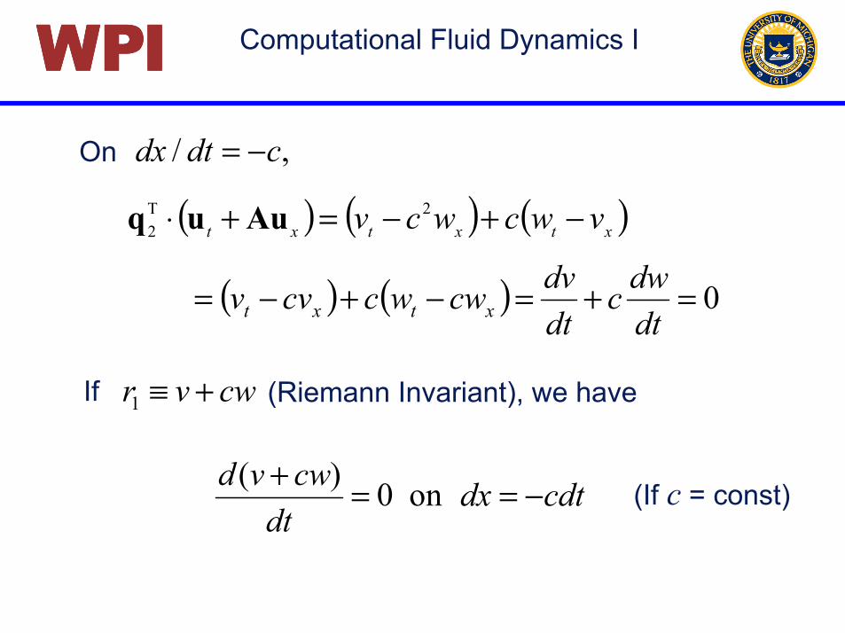
Computational Fluid Dynamics IPPPPIIIIWWWWOn ,/ cdtdx +=
( ) ( ) ( )xtxtxt vwcwcv −−−=+⋅ 2T1 Auuq
( ) ( ) 0=−=+−+=dtdwc
dtdvcwwccvv xtxt
If cwvr −≡1 (Riemann Invariant), we have
cdtdxdt
cwvd +==− on0)((If c = const)
Computational Fluid Dynamics IPPPPIIIIWWWWOn ,/ cdtdx −=
( ) ( ) ( )xtxtxt vwcwcv −+−=+⋅ 2T2 Auuq
( ) ( ) 0=+=−+−=dtdwc
dtdvcwwccvv xtxt
If cwvr +≡1 (Riemann Invariant), we have
cdtdxdt
cwvd −==+ on0)((If c = const)

Computational Fluid Dynamics IPPPPIIIIWWWW
Pcdtdx +=/
cdtdx −=/
cdtdxdtdwc
dtdv +==− on0
cdtdxdtdwc
dtdv −==+ on0
1
2
3
known,,xf
tff
∂∂
∂∂
dxfdtfdf xt +=
Computational Fluid Dynamics IPPPPIIIIWWWW
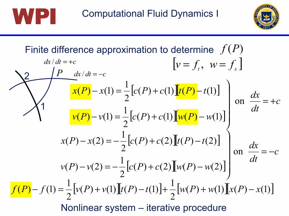
[ ][ ] [ ][ ])1()()1()(21)1()()1()(
21)1()( xPxwPwtPtvPvfPf −++−+=−
[ ][ ]
[ ][ ]
−+=−
−+=−
)1()()1()(21)1()(
)1()()1()(21)1()(
wPwcPcvPv
tPtcPcxPx
Finite difference approximation to determine )(Pf[ ]xt fwfv == ,
P cdtdx −=/
1
2cdtdx +=/
cdtdx +=on
[ ][ ]
[ ][ ]
−+−=−
−+−=−
)2()()2()(21)2()(
)2()()2()(21)2()(
wPwcPcvPv
tPtcPcxPxc
dtdx −=on
Nonlinear system – iterative procedure

Computational Fluid Dynamics IPPPPIIIIWWWW
Numerical Methods:Finite Volume Approach

Computational Fluid Dynamics IPPPPIIIIWWWW
When using finite volume approximations, we work directly with the integral form of the conservation principles. The average values of f over a small volume are stored
xj−1/2 xj+1/2
1−jfjf
x
f
1+jf

Computational Fluid Dynamics IPPPPIIIIWWWWIn finite volume method, equations in conservative forms are needed in order to satisfy conservation properties.
As an example, consider a 1-D equation
0)],([),( =∂
∂+∂
∂x
txfFt
txf
where F denotes a general advection/diffusion term, e.g.
xfxFfF∂∂== )(;
21 2 µ

Computational Fluid Dynamics IPPPPIIIIWWWW
0=∂∂+
∂∂
∫∫LL
dxxFdx
tf
0)0()( =− FLF
0=⇒ ∫L
fdxdtd
If F = 0 at the end points of the domain, f is conserved.
Integrating over the domain L,
Computational Fluid Dynamics IPPPPIIIIWWWW
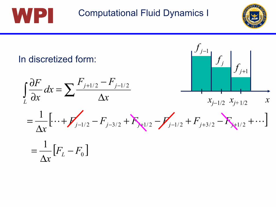
∑∫ ∆−
=∂∂ −+
xFF
dxxF jj
L
2/12/1
xj−1/2 xj+1/2
1+jf
1−jfjf
x
In discretized form:
[ ]!! +−+−+−+∆
= ++−+−− 2/12/32/12/12/32/11
jjjjjj FFFFFFx
[ ]01 FFx L −∆
=

Computational Fluid Dynamics IPPPPIIIIWWWW
0)(,021 2 =
∂∂
∂∂+
∂∂=
∂∂+
∂∂
xfx
xtff
xtf µ
Examples of Conservative Form
Discretize
( )( ) ( )( )[ ]11112
2/12/1
21
1
−−++
−+
−+−−+
=
∂∂−
∂∂
jjjjjjjj
jj
ffffh
xf
xf
h
µµµµ
µµ
∂∂
∂∂
xfx
x)(µ
Conservative

Computational Fluid Dynamics IPPPPIIIIWWWWExamples of Non-conservative Form
Discretize
0,0 2
2
=∂∂
∂∂+
∂∂+
∂∂=
∂∂+
∂∂
xf
xxf
tf
xff
tf µµ
xf
xxf
∂∂
∂∂+
∂∂ µµ 2
2
( ) ( )( )
( ) ( )
+−−+−+
=
−−+−+
−−+−−+++−+
−+−+−+
11111111112
1111112
4121
4121
jjjjjjjjjjjjjj
jjjjjjjj
fffffffh
fffffh
µµµµµµµ
µµµ
Non-conservative

Computational Fluid Dynamics IPPPPIIIIWWWW
0=∂∂+
∂∂
xF
tf
F = Uf Advection
Diffusion
Advection/Diffusion
xfDF∂∂=
xfDUfF∂∂−=
Finite Volume Method for Conservative Equations

Computational Fluid Dynamics IPPPPIIIIWWWW
0=∂∂+
∂∂
xF
tf
0=∂∂+
∂∂
∫∫∆∆
dxxFdx
tf
xx
02/12/1 =−+ −+∆∫ jjx
FFdxfdtd
0)( 2/12/1 =−+ −+ jjj FFhfdtd
Fj−1/2 Fj+1/2
1−jf
x
Finite Volume Formulation
j j+1j−1
jf1+jf

Computational Fluid Dynamics IPPPPIIIIWWWW
∂∂−
∂∂+−−=
−+−+
2/12/12/12/1 )(
jjjjj x
fxfDffUf
dtdh
)(21
12/1nj
njj fff +≈ ++
hff
xf n
jnj
j
−≈
∂∂ +
+
1
2/1
)(1 1 nj
njj ff
tf
dtd −
∆≈ +
Approximating
1-D Advection-Diffusion Equation
0=
∂∂−
∂∂+
∂∂
xfDUf
xtf
FVM Equation:
Computational Fluid Dynamics IPPPPIIIIWWWW
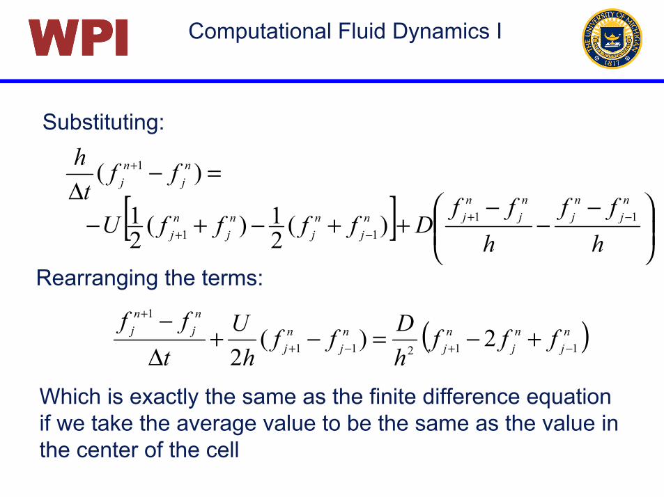
=−∆
+ )( 1 nj
nj ff
th
( )nj
nj
nj
nj
nj
nj
nj fff
hDff
hU
tff
11211
1
2)(2 −+−+
+
+−=−+∆−
Rearranging the terms:
Substituting:
Which is exactly the same as the finite difference equation if we take the average value to be the same as the value in the center of the cell
[ ]
−−
−++−+− −+
−+ hff
hff
DffffUnj
nj
nj
njn
jnj
nj
nj
1111 )(2
1)(21

Computational Fluid Dynamics IPPPPIIIIWWWW
Numerical Methods for 1-D Advection Equation:Stability Consideration
(Finite Difference Approach)

Computational Fluid Dynamics IPPPPIIIIWWWW
We will start by examining the linear advection equation:
0=∂∂+
∂∂
xfU
tf
The characteristic for this equation are:
;0; ==dtdfU
dtdx
Showing that the initial conditions are simply advected by a constant velocity U
t
f
f
x

Computational Fluid Dynamics IPPPPIIIIWWWW
A forward in time, centered in space (FTCS) discretization yields
0=∂∂+
∂∂
xfU
tf
)(2 11
1 nj
nj
nj
nj ffU
htff −+
+ −∆−=
j−1 j j+1n
n+1
Finite difference equation
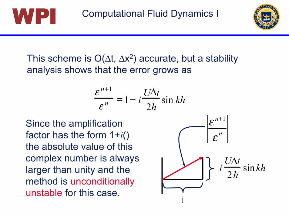
Computational Fluid Dynamics IPPPPIIIIWWWWThis scheme is O(∆t, ∆x2) accurate, but a stability analysis shows that the error grows as
ε n+1
ε n =1− iU∆t2h
sin kh
Since the amplification factor has the form 1+i() the absolute value of this complex number is always larger than unity and the method is unconditionally unstable for this case.
iU∆t2h
sin kh
1
ε n+1
ε n

Computational Fluid Dynamics IPPPPIIIIWWWW
A forward in time but “upwind” (windward) in space discretization yields
)( 11 n
jnj
nj
nj ffU
htff −
+ −∆−=
j−1 jn
n+1 This scheme is O(∆t, ∆x) accurate.
0=∂∂+
∂∂
xfU
tf
Alternative Scheme: Upwind Difference1−jf jf 1+jf
U

Computational Fluid Dynamics IPPPPIIIIWWWWTo examine the stability we use the von Neuman’s method:
nj
nj
nj ff ε+=
0)( 1
1
=−+∆−
−
+nj
nj
nj
nj
hU
tεε
εε
jikxnnj eεε =
0)1(1
=−+∆− −
+ikh
nnn
eh
Ut
εεε
Substituting into the modified equation,
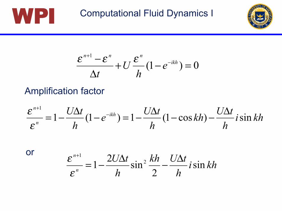
Computational Fluid Dynamics IPPPPIIIIWWWW
0)1(1
=−+∆− −
+ikh
nnn
eh
Ut
εεε
khih
tUkhh
tUeh
tU ikhn
n
sin)cos1(1)1(11 ∆−−∆−=−∆−= −+
εε
Amplification factor
khih
tUkhh
tUn
n
sin2
sin21 21 ∆−∆−=+
εεor
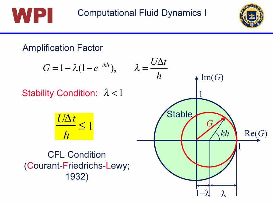
Computational Fluid Dynamics IPPPPIIIIWWWW
htUeG ikh ∆=−−= − λλ ),1(1
Amplification Factor
Stable
Re(G)
Im(G)
1
1
kh
λ1−λ
Stability Condition:
U∆th
≤ 1
CFL Condition(Courant-Friedrichs-Lewy;
1932)
G
1<λ
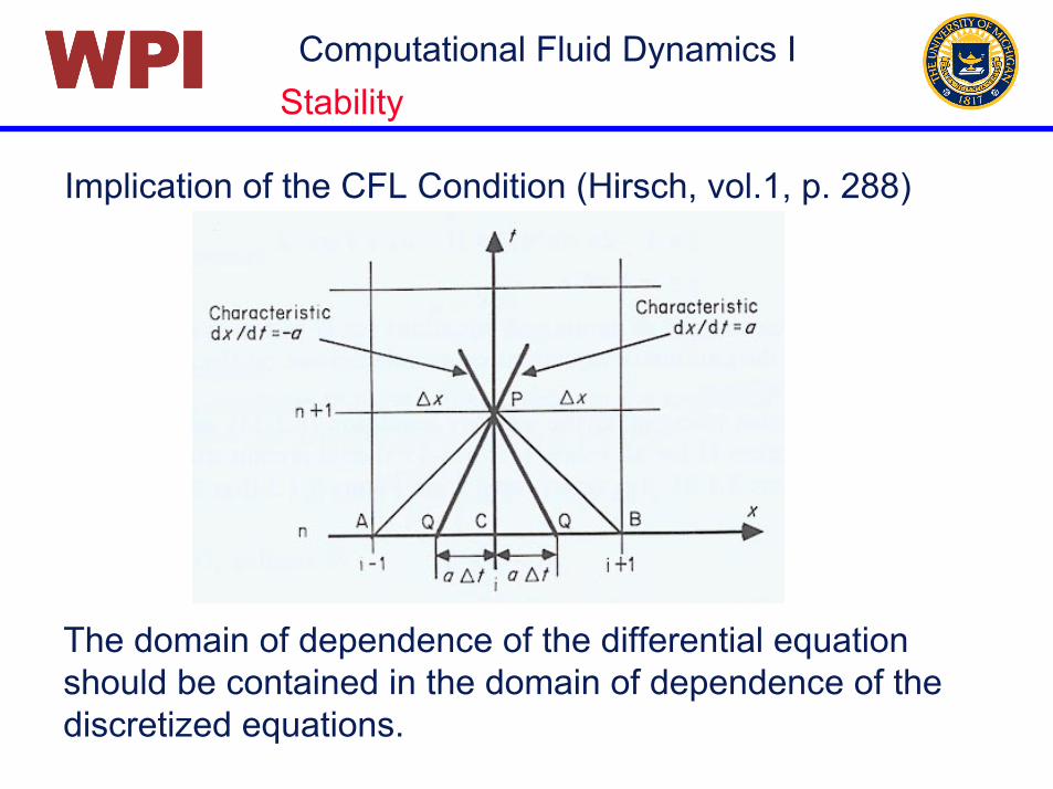
Computational Fluid Dynamics IPPPPIIIIWWWWImplication of the CFL Condition (Hirsch, vol.1, p. 288)
Stability
The domain of dependence of the differential equation should be contained in the domain of dependence of the discretized equations.

Computational Fluid Dynamics IPPPPIIIIWWWW
Stability Consideration(Finite Volume Approach)

Computational Fluid Dynamics IPPPPIIIIWWWW
0=∂∂+
∂∂
xF
tf
0=∂∂+
∂∂
∫∫∆∆
dxxFdx
tf
xx
02/12/1 =−+ −+∆∫ jjx
FFdxfdtd
( ) ( ) 02/12/11 =−∆+− −++ n
jnj
nj
nj FFtffh
Finite Volume Formulation
Fj-1/2 Fj+1/2
1+jf
f j−1
jf
xj j+1j-1
( )nj
nj
nj
nj FF
htff 2/12/1
1−+
+ −∆−=

Computational Fluid Dynamics IPPPPIIIIWWWW
UffF jjj )(21
12/1 +≈ ++
UfF jj ≈+ 2/1
Approximating the advective fluxes:
Taking the average (Central):
Upwind:
1+jf
f j−1
jf
xj j+1j-1
U
( ) ( )
+−+∆−= −+
+ nj
nj
nj
nj
nj
nj ffUffU
htff 11
1
22
( )nj
nj
nj
nj UfUf
htff 1
1−
+ −∆−=
[ ]nj
nj
nj UfUf
htf 112 −+ −∆−=

Computational Fluid Dynamics IPPPPIIIIWWWW
1+jf
Consider the following initial conditions:
1
1−jf jf
0.1)(2 12/1 =+= −−
nj
nj
nj ffUF 5.0)(
2 12/1 =+= ++nj
nj
nj ffUF
25.1)15.0(5.00.1)( 2/12/11 =−−=−∆−= −++ n
jnj
nj
nj FF
htff
Central Differencing and Stability
25.0)5.00(5.00)( 2/12/311
1 =−−=−∆−= +++++
nj
nj
nj
nj FF
htff
5.0
0.1
=∆=
ht
U

Computational Fluid Dynamics IPPPPIIIIWWWW
1+jf
Next time step (n+2):
1
1−jf jf
125.1)(2
111
12/1 =+= ++
−+−
nj
nj
nj ffUF 75.0)(
21
111
2/1 =+= ++
+++
nj
nj
nj ffUF
3125.1)125.175.0(5.0125.1)( 12/1
12/1
12 =−−=−∆−= +−
++
++ nj
nj
nj
nj FF
htff
Central Differencing and Stability
5.0
0.1
=∆=
ht
U
Cell j will overflow immediately !!!

Computational Fluid Dynamics IPPPPIIIIWWWWBy considering the fluxes, it is easy to see why the centered difference approximation is always unstable.
nj
nj
nj
ni
ni
nj
nj
ffhtUf
UfUfhtff
>∆+=
−∆−=+
2
211
1+jf
1
1−jf jf
nj
nj ff >+1 Always !

Computational Fluid Dynamics IPPPPIIIIWWWW
Consider the following initial conditions:
U
Upwind Differencing and Stability
1+jf1
1−jf jf
Computational Fluid Dynamics IPPPPIIIIWWWW
U1+jf
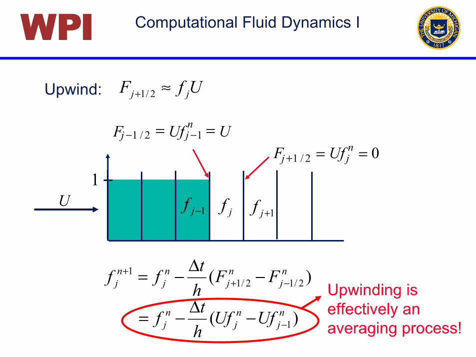
1
1−jf jf
UfF jj ≈+ 2/1Upwind:
Fj−1 / 2 = Ufj−1n = U
Fj+1 / 2 = Ufjn = 0
)( 2/12/11 n
jnj
nj
nj FF
htff −+
+ −∆−=
)( 1nj
nj
nj UfUf
htf −−∆−=
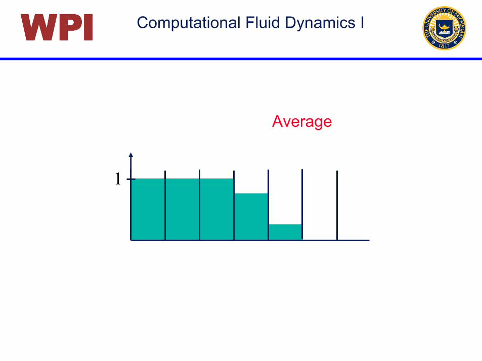
Upwinding iseffectively anaveraging process!

Computational Fluid Dynamics IPPPPIIIIWWWW
1
Average

Computational Fluid Dynamics IPPPPIIIIWWWW
Advect
1
Computational Fluid Dynamics IPPPPIIIIWWWW
1
Average

Computational Fluid Dynamics IPPPPIIIIWWWW
1
Advect

Computational Fluid Dynamics IPPPPIIIIWWWW
1
Average

Computational Fluid Dynamics IPPPPIIIIWWWW
1
Advect

Computational Fluid Dynamics IPPPPIIIIWWWW
1−jf jf 1+jf
112/1 == −−njj UfF
02/1 ==+njj UfF
Consider the following initial conditions:
1
During one time step, U∆t of f flows into cell j, increasing the average value of f by U∆t/h.
Upwind Differencing: Unstable Case

Computational Fluid Dynamics IPPPPIIIIWWWW
1+jf
Integration using upwind scheme:
1
1−jf jf
Fj−1 / 2 = Ufj−1n = U
Fj+1 / 2 = Ufjn = 0
5.1)10(5.10)( 2/12/11 =−−=−∆−= −++ n
jnj
nj
nj FF
htff
1=U 5.1=∆ht
>∆ 1
htU

Computational Fluid Dynamics IPPPPIIIIWWWW
1+jf1
1−jf jf
Fj−1 / 2 = Ufj−1n =U Fj+1 / 2 = Ufj
n = 1.5U
75.0)15.1(5.10)( 2/12/11 =−−=−∆−= −++ n
jnj
nj
nj FF
htff
25.2)5.10(5.10)( 2/12/311
1 =−−=−∆−= +++++
nj
nj
nj
nj FF
htff

Computational Fluid Dynamics IPPPPIIIIWWWW
1+jf1
1−jf jf
Fj−1 / 2 = Ufj−1n =U
Fj+1 / 2 = Ufjn = 0.75U
Taking a third step will result in an even larger positive value, and so on until the compute encounters a NaN (Not a Number).
Fj+1 / 2 = Ufjn = 2.25U

Computational Fluid Dynamics IPPPPIIIIWWWW
If U∆t/h > 1, the average value of f in cell j will be larger than in cell j−1. In the next step, f will flow out of cell j in both directions, creating a larger negative value of f. Taking a third step will result in an even larger positive value, and so on until the compute encounters a NaN (Not a Number).

Computational Fluid Dynamics IPPPPIIIIWWWW
Consideration of Modified Equations:
Why is upwind scheme stable?(Ref: Tannehill et al., Ch. 4)

Computational Fluid Dynamics IPPPPIIIIWWWWDerive modified equation for upwind difference method:
0)( 1
1
=−+∆−
−
+nj
nj
nj
nj ff
hU
tff
Using Taylor expansion:
!+∆∂∂+∆
∂∂+∆
∂∂+=+
62
3
3
32
2
21 t
tft
tft
tfff n
jnj
!+∂∂−
∂∂+
∂∂−=− 62
3
3
32
2
2
1
hxfh
xfh
xfff n
jnj

Computational Fluid Dynamics IPPPPIIIIWWWWSubstituting
−
+∆
∂∂+∆
∂∂+∆
∂∂+
∆nj
nj ft
tft
tft
tff
t!
621 3
3
32
2
2
062
3
3
32
2
2
=
+
∂∂−
∂∂+
∂∂−−+ !
hxfh
xfh
xfff
hU n
jnj
Therefore,
!+−∆−+∆−=∂∂+
∂∂
xxxtttxxtt fUhftfUhftxfU
tf
6622
22
It helps the interpretation if all terms are written in xxxxx ff ,

Computational Fluid Dynamics IPPPPIIIIWWWWTaking further derivatives:
!+−∆−+∆−=+ xxxtttttxxttttxttt fUhftfUhftUff6622
22
!++∆+−∆=−− xxxxtttxxxxttxxxtx fhUftUfhUftUfUUf6622
22222+
+−∆+
∆++−∆+=
)(22
)(22
2
2
hOuUuUx
tOfUftfUf
xxxxxt
ttxttt
xxtt

Computational Fluid Dynamics IPPPPIIIIWWWWSimilarly, we get
),(3 htOfUf xxxttt ∆+−=
),(2 htOfUf xxxttx ∆+=
),( htOUff xxxxxt ∆+−=
Final form of the modified equation:
( ) ( ) xxxxx fUhfUhxfU
tf 132
61
22
2
+−−−=∂∂+
∂∂ λλλ
[ ]3223 ,,, tththhO ∆∆∆+
htU∆=λ
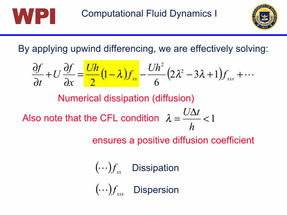
Computational Fluid Dynamics IPPPPIIIIWWWW
Numerical dissipation (diffusion)
( ) ( ) !++−−−=∂∂+
∂∂
xxxxx fUhfUhxfU
tf 132
61
22
2
λλλ
By applying upwind differencing, we are effectively solving:
Also note that the CFL condition 1<∆=h
tUλ
ensures a positive diffusion coefficient
Dissipation( ) xxf!
Dispersion( ) xxxf!

Computational Fluid Dynamics IPPPPIIIIWWWWDissipation vs. Dispersion
Exact Dissipative Dispersive
The nature of the numerical scheme depends on thenature of the lowest order truncation error term.

Computational Fluid Dynamics IPPPPIIIIWWWWGeneralized Upwind Scheme (for both U > 0 and U < 0 )
0),( 11 >−∆−= −+ Uff
htUff n
jnj
nj
nj
0),( 11 <−∆−= ++ Uff
htUff n
jnj
nj
nj
Define( ) ( )UUUUUU −=+= −+
21,
21
The two cases can be combined into a single expression:
[ ])()( 111 n
jnj
nj
nj
nj
nj ffUffU
htff −+−∆−= +
−−
++

Computational Fluid Dynamics IPPPPIIIIWWWW
Or, substituting
; General representation of various flux formula
)2(2
)(2 1111
1 nj
nj
nj
nj
nj
nj
nj fff
htU
ffhtUff −+−+
+ +−∆
+−∆−=
−+ UU ,
central difference + artificial viscosity
=
2hU
α

Computational Fluid Dynamics IPPPPIIIIWWWW
While the first-order upwind scheme was found to bestable, it is in general too dissipative (smoothes out all the steep gradients).
Stable and accurate methods:- Lax-Wendroff (I and II)- Leapfrog- Lax-Friedrichs- MacCormack- 2nd order upwind- etc., etc., …

Computational Fluid Dynamics IPPPPIIIIWWWW1. Implicit (Backward Euler) Method
- Unconditionally stable- 1st order in time, 2nd order in space- Forms a tri-diagonal matrix (Thomas algorithm)
( ) 02
11
11
1
=−+∆− +
−++
+nj
nj
nj
nj ff
hU
tff
nj
nj
nj
nj f
tf
hUf
tf
hU
∆=−
∆+ +
−++
+
12
12
11
111
jnjj
njj
njj Cfbfdfa =++ +
−++
+1
111
1
Implicit Method

Computational Fluid Dynamics IPPPPIIIIWWWWThomas Algorithm
⋅⋅⋅
=
⋅⋅⋅
⋅⋅
⋅⋅⋅⋅⋅⋅
⋅⋅⋅
−
+
+−
+
+
−−−
M
M
nM
nM
n
n
MM
MMM
CC
CC
ff
ff
dbadb
adbadb
ad
1
2
1
1
11
12
11
111
333
222
11
000
0
00
jnjj
njj
njj Cfbfdfa =++ +
−++
+1
111
1
Implicit Method

Computational Fluid Dynamics IPPPPIIIIWWWWThomas Algorithm – The Algorithm
Mjadb
dd jj
jjj ,,3,21
1
!=−= −−
MjCdb
CC jj
jjj ,,3,21
1
!=−= −−
1,,2,11
11 !−−=−=+++ MMk
dfaCf
k
nkkkn
j
Forward Sweep:
Backward Sweep:
Implicit Method

Computational Fluid Dynamics IPPPPIIIIWWWW
( ) 2/11nj
nj
nj fff −+ +→
2. Lax (Lax-Friedrichs) Method
The forward Euler method can be made stable by
Modified equation
( ) ( )nj
nj
nj
nj
nj ff
htUfff 1111
1
221
−+−++ −∆−+=
( ) !+−+
−=
∂∂+
∂∂
xxxxx fUhfUhxfU
tf 2
2
13
12
λλλ
- Stable for 1<λ- Not uniformly consistent - Still 1st order (dissipative)
( )htU /∆=λ
Lax Method

Computational Fluid Dynamics IPPPPIIIIWWWW
)(2
211
tOtff
tf n
jnj ∆+
∆−
=∂∂ −+
3. Leap Frog Method
The simplest stable second-order accurate (in time) method:
Modified equation
( )nj
nj
nj
nj ff
htUff 11
11−+
−+ −∆−=
( ) !+−=∂∂+
∂∂
xxxfUhxfU
tf 1
62
2
λ
- Stable for 1<λ- Dispersive (no dissipation) – error will not damp out- Initial conditions at two time levels - Oscillatory solution in time (alternating)
Leap Frog Method

Computational Fluid Dynamics IPPPPIIIIWWWW
!+∆∂∂+∆
∂∂+∆
∂∂+=∆+
62)()(
3
3
32
2
2 ttft
tft
tftfttf
4. Lax-Wendroff’s Method (LW-I)
First expand the solution in time
Then use the original equation to rewrite the time derivatives
xfU
tf
∂∂−=
∂∂
2
22
2
2
xfU
tf
xU
xfU
ttf
ttf
∂∂=
∂∂
∂∂−=
∂∂
∂∂−=
∂∂
∂∂=
∂∂
LW-I Method

Computational Fluid Dynamics IPPPPIIIIWWWW
)(2
)()( 32
2
22 tOt
xfUt
xfUtfttf ∆+∆
∂∂+∆
∂∂−=∆+
Substituting
Using central differences for the spatial derivatives
( ) ( )nj
nj
nj
nj
nj
nj
nj fff
htUff
htUff 112
22
111 2
22 −+−++ +−∆+−∆−=
2nd order accurate in space and time
Stable for 1<∆h
tU
LW-I Method

Computational Fluid Dynamics IPPPPIIIIWWWW5. Two-Step Lax-Wendroff’s Method (LW-II)
LW-I into two steps:
For the linear equations, LW-II is identical to LW-I (prove it!)
02/
2/)( 112/1
2/1 =−
+∆
+− ++++
hff
Ut
fff nj
nj
nj
nj
nj
02/1
2/12/1
2/11
=−
+∆− +
−++
+
hff
Ut
ff nj
nj
nj
nj
Step 1 (Lax)
Step 2 (Leapfrog)
- Stable for 1/ <∆ htU- Second order accurate in time and space
LW-II Method

Computational Fluid Dynamics IPPPPIIIIWWWW6. MacCormack Method
Similar to LW-II, without
( )nj
nj
nj
tj ff
htUff −∆−= +1
( )
−∆−+= −
+ tj
tj
tj
nj
nj ff
htUfff 1
1
21
Predictor
Corrector
- A fractional step method- Predictor: forward differencing- Corrector: backward differencing
- For linear problems, accuracy and stability properties areidentical to LW-I.
2/1,2/1 −+ jj
MacCormack Method

Computational Fluid Dynamics IPPPPIIIIWWWW7. Second-Order Upwind Method
Warming and Beam (1975) – Upwind for both steps
( )nj
nj
nj
tj ff
htUff 1−−∆−=
( ) ( )
+−∆−−∆−+= −−−
+ nj
nj
nj
tj
tj
tj
nj
nj fff
htUff
htUfff 211
1 221
Predictor Corrector
Combining the two:
( ) ( )nj
nj
nj
nj
nj
nj
nj fffffff 211
1 2)1(21
−−−+ +−−+−−= λλλ
2nd Order Upwind Method
- Stable if- Second-order accurate in time and space
20 ≤≤ λ

Computational Fluid Dynamics IPPPPIIIIWWWW
And the list goes on…

Computational Fluid Dynamics IPPPPIIIIWWWW
Conditionally consistent
Stable for
Lax-Friedrichs
UnconditionallyStable
Implicit
Stable forUpwind
Unconditionally Unstable
FTCS
0=+ xt Uff
02
111
=−
+∆− −+
+
hff
Ut
ff nj
nj
nj
nj ( ) xxxxx fUhfUt 2
22
2162
λ+−∆−
011
=−
+∆− −
+
hff
Ut
ff nj
nj
nj
nj
( )
( ) xxx
xx
fUh
fUh
1326
12
22
+−−
−
λλ
λ
1≤λ
( ) xxxxx fUhfUh 22
13
12
λλλ
−+
−
( )0
2
11
11
1
=−
+∆− +
−++
+
hff
Ut
ff nj
nj
nj
nj
xxxxx ftUUhftU
∆+−∆ 232
2
31
61
2
( )
( )0
2
2/
11
111
=−
+
∆+−
−+
−++
hff
U
tfff
nj
nj
nj
nj
nj
1≤λ

Computational Fluid Dynamics IPPPPIIIIWWWW
Stable forSame as LW-I
MacCormack
Stable forSame as LW-I
Lax-Wendroff II
Stable forLax-Wendroff I
Stable forLeap Frog
0=+ xt Uff
022
1111
=−
+∆− −+
−+
hff
Utff n
jnj
nj
nj ( ) xxxfUh 1
62
2
−λ
( )
( ) xxxx
xxx
fUh
fUh
23
22
18
16
λλ
λ
−−
−−
1≤λ
1≤λ
1≤λ
( )
( )0
22
2
2
1122
111
=+−
∆−
−+
∆−
−+
−++
hfff
tU
hff
Ut
ff
nj
nj
nj
nj
nj
nj
nj
02/
2/)( 112/1
2/1 =−
+∆
+− ++++
hff
Ut
fff nj
nj
nj
nj
nj
02/1
2/12/1
2/11
=−
+∆− +
−++
+
hff
Ut
ff nj
nj
nj
nj 1≤λ
( )01 =
−+
∆− +
hff
Utff n
jnj
nj
tj
( ) ( )0
2/ 11
=−
+∆+− −
+
hff
Ut
fff tj
tj
tj
nj
nj
Computational Fluid Dynamics IPPPPIIIIWWWW
Closing Remarks

Computational Fluid Dynamics IPPPPIIIIWWWW
Summary by CFD School A
“In solving inviscid flow equations as found in manygas dynamic applications, central differencing scheme is inherently unstable and thus cannot be used. One should use more robust methods such as upwind or other higher order methods in order to ensure stability and accuracy. In general, central differencing scheme is a deficient method in capturing true physical behaviorand should be avoided if at all possible.”

Computational Fluid Dynamics IPPPPIIIIWWWW
Summary by CFD School B
“Upwind-type schemes applied to the Navier-Stokes equations inherently introduce numerical dissipation which depends on numerical parameters, not on actual physical processes. Sometimes these uncontrolled numerical dissipation may interfere withphysical solution, thereby degrading the fidelity ofsimulation. Central differencing does not suffer fromartificial dissipation and thus preferred as an accuratenumerical method.”