Embed Size (px)
Citation preview

Computational Fluid Dynamics IPPPPIIIIWWWW
Numerical Methods forWave Equation:
Part II: Discontinuous Solutions
Instructor: Hong G. ImUniversity of Michigan
Fall 2001

Computational Fluid Dynamics IPPPPIIIIWWWW
Part I• Method of Characteristics• Finite Volume Approach and Conservative Forms• Methods for Continuous Solutions
- Central and Upwind Difference- Stability, CFL Condition- Various Stable Methods
Part II• Methods for Discontinuous Solutions
- Burgers Equation and Shock Formation- Entropy Condition- Various Numerical Schemes
Outline
Solution Methods for Wave Equation

Computational Fluid Dynamics IPPPPIIIIWWWW
Exact Solutions

Computational Fluid Dynamics IPPPPIIIIWWWW
0=∂∂+
∂∂
xfc
tf
The analytic solution is obtained by characteristics
;0; ==dtdfc
dtdx
Consider 1st Order Wave Equation
t
f
f
xDiscontinuity of solution is allowed
(Weak Solution)
( )RLR
L ffxxfxxf
xf >
><
=0
0)0,(
cdtdx =

Computational Fluid Dynamics IPPPPIIIIWWWW
( )RLR
L ffxxfxxf
xf >
><
=0
0)0,(0=∂∂+
∂∂
xff
tf
;0; ==dtdff
dtdx
Inviscid Burgers’ Equation
t
x
Characteristics
0x
Lf
Rf
??=dtdx
0x
Shock Wave
Computational Fluid Dynamics IPPPPIIIIWWWW
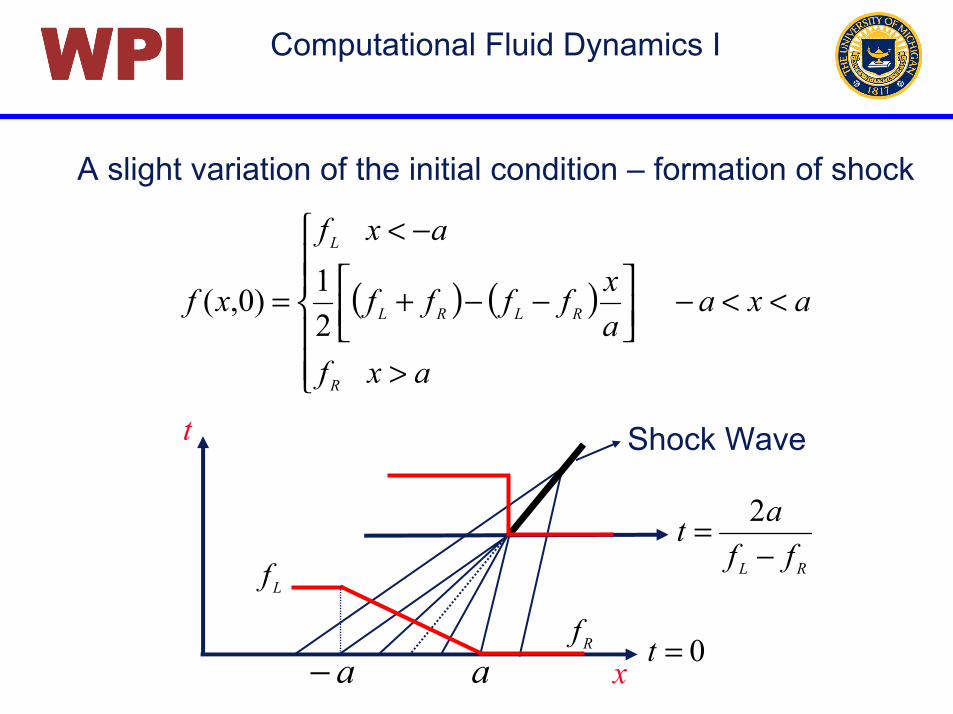
( ) ( ) axa
axfaxffff
axf
xf
R
RLRL
L
<<−
>
−−+
−<
=21)0,(
A slight variation of the initial condition – formation of shock
t
x
Shock Wave
a− a
Lf
Rf 0=t
RL ffat−
= 2

Computational Fluid Dynamics IPPPPIIIIWWWW
( )RLR
L ffxxfxxf
xf <
><
=0
0)0,(0=∂∂+
∂∂
xff
tf
;0; ==dtdff
dtdx
Reverse Shock (?)
Characteristics
0x
Lf
Rf t
x0x
Unstable, entropy-violatingsolution
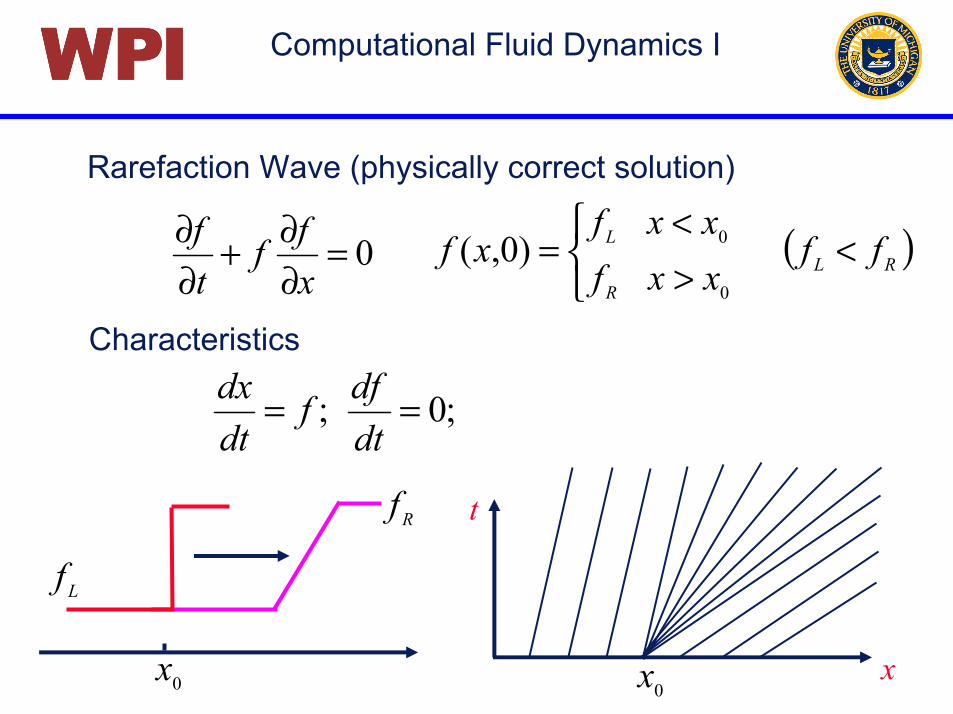
Computational Fluid Dynamics IPPPPIIIIWWWW
( )RLR
L ffxxfxxf
xf <
><
=0
0)0,(0=∂∂+
∂∂
xff
tf
;0; ==dtdff
dtdx
Rarefaction Wave (physically correct solution)
Characteristics
0x
Lf
Rf t
x0x
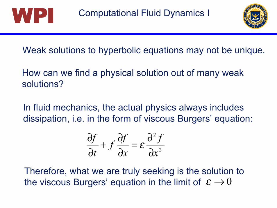
Computational Fluid Dynamics IPPPPIIIIWWWWWeak solutions to hyperbolic equations may not be unique.
How can we find a physical solution out of many weaksolutions?
In fluid mechanics, the actual physics always includes dissipation, i.e. in the form of viscous Burgers’ equation:
2
2
xf
xff
tf
∂∂=
∂∂+
∂∂ ε
Therefore, what we are truly seeking is the solution to the viscous Burgers’ equation in the limit of 0→ε

Computational Fluid Dynamics IPPPPIIIIWWWWIn CFD, however, we do not want to solve the viscousBurgers’ equation with extremely small because it becomes computationally expensive.
Nevertheless, in many gas dynamics application, thereis need to capture discontinuous solution behavior.
And we want to reproduce the weak solution behaviornumerically by solving inviscid Burgers’ equation.
ε
- Shock speed- Entropy condition- Wave shape (without smearing or wiggles)
Computational Fluid Dynamics IPPPPIIIIWWWW
Finite Difference Methodsfor
Discontinuous Solutions
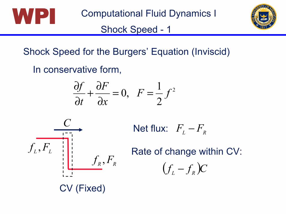
Computational Fluid Dynamics IPPPPIIIIWWWWShock Speed for the Burgers’ Equation (Inviscid)
In conservative form,
2
21,0 fF
xF
tf ==
∂∂+
∂∂
LL Ff ,RR Ff ,
C
CV (Fixed)
Net flux: RL FF −
Rate of change within CV:
( )Cff RL −
Shock Speed - 1
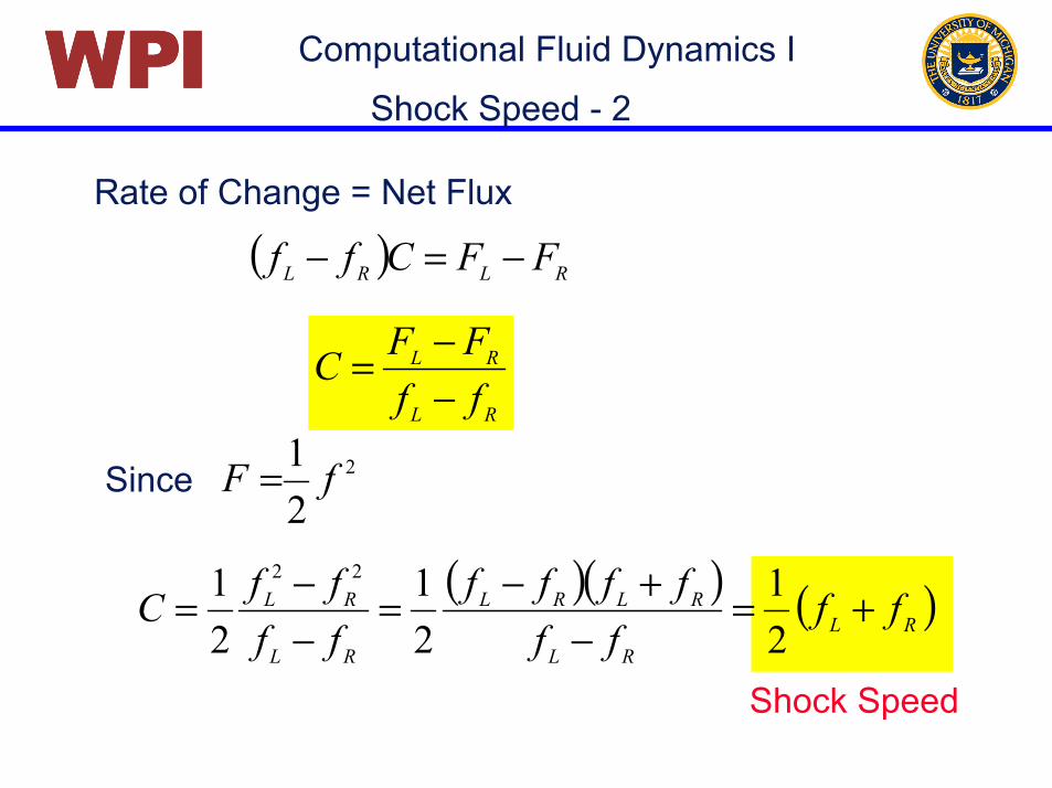
Computational Fluid Dynamics IPPPPIIIIWWWWRate of Change = Net Flux
( ) RLRL FFCff −=−
RL
RL
ffFFC
−−=
Since 2
21 fF =
( )( ) ( )RLRL
RLRL
RL
RL ffff
ffffffffC +=
−+−=
−−=
21
21
21 22
Shock Speed
Shock Speed - 2

Computational Fluid Dynamics IPPPPIIIIWWWW
In capturing the correct solution behavior for discontinuousInitial data, conservative methods are essential.
Conservative Methods for Nonlinear Problems
Example: inviscid Burgers equation:
021or0 2 =
∂∂+
∂∂=
∂∂+
∂∂ f
xtf
xff
tf
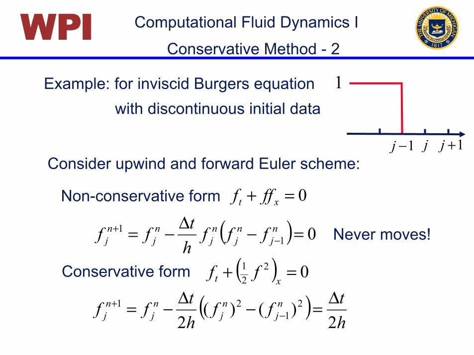
Conservative Method - 1
Computational Fluid Dynamics IPPPPIIIIWWWW
Consider upwind and forward Euler scheme:
Example: for inviscid Burgers equationwith discontinuous initial data
0=+ xt fff
1−j
1
j 1+j
( ) 011 =−∆−= −+ n
jnj
nj
nj
nj fff
htff
Non-conservative form
Never moves!
( ) 0221 =+
xt ff
( )htff
htff n
jnj
nj
nj 2
)()(2
21
21 ∆=−∆−= −+
Conservative form
Conservative Method - 2

Computational Fluid Dynamics IPPPPIIIIWWWW
Entropy Condition:A discontinuity propagating with speed C satisfies the entropy condition if
For a conservation equation
)()( RL fFCfF ′>>′
( ) ( ) ( ) ( )R
R
L
L
fffFfFC
fffFfF
−−≥≥
−−
Entropy Condition - 1
0)( =∂
∂+∂∂
xfF
tf
Version I
Version II
And some others…

Computational Fluid Dynamics IPPPPIIIIWWWW
Examples: Godunov methodApproximate Riemann solverArtificial dissipation
In practice, rather than applying a separate entropy condition to the numerical solution procedure, numericalmethods are developed first and then it can be provedthat the methods satisfy the entropy condition.
Entropy Condition - 2
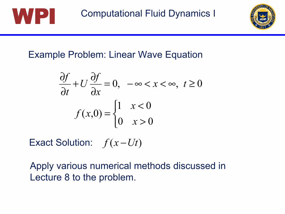
Computational Fluid Dynamics IPPPPIIIIWWWWExample Problem: Linear Wave Equation
0,,0 ≥∞<<∞−=∂∂+
∂∂ tx
xfU
tf
><
=0001
)0,(xx
xf
Exact Solution: )( Utxf −
Apply various numerical methods discussed in Lecture 8 to the problem.

Computational Fluid Dynamics IPPPPIIIIWWWW
Stable forBeam-Warming
Stable forLax-Wendroff I
Conditionally consistent
Stable for
Lax-Friedrichs
Stable forUpwind
0=+ xt Uff
1≤λ
( )
( ) 022
243
212
2
211
=+−∆−
+−+
∆−
−−
−−+
nj
nj
nj
nj
nj
nj
nj
nj
fffh
tUh
fffU
tff
20 ≤≤ λ
011
=−
+∆− −
+
hff
Ut
ff nj
nj
nj
nj
( )
( ) xxx
xx
fUh
fUh
1326
12
22
+−−
−
λλ
λ
1≤λ
( ) xxx
xx
fUh
fUh
22
13
12
λ
λλ
−+
−
( )
( )0
2
2/
11
111
=−
+
∆+−
−+
−++
hff
U
tfff
nj
nj
nj
nj
nj
( )
( ) xxxx
xxx
fUh
fUh
23
22
18
16
λλ
λ
−−
−−( )
( )0
22
2
2
1122
111
=+−
∆−
−+
∆−
−+
−++
hfff
tU
hff
Ut
ff
nj
nj
nj
nj
nj
nj
nj
1≤λ
( )( )
( ) ( ) xxxx
xxx
fUh
fUh
λλ
λλ
−−−
−−
218
216
23
2

Computational Fluid Dynamics IPPPPIIIIWWWWComparison: 5.0at;01.0 == th
LeVeque, R. J., Numerical Methods for Conservation Laws, Birkhäuser, 1992
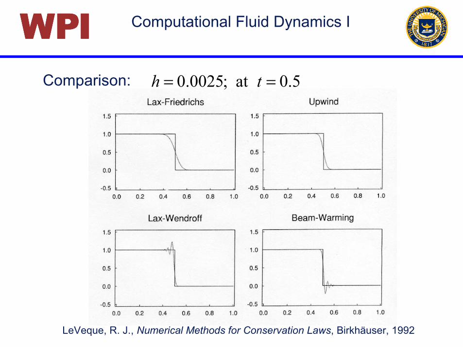
Computational Fluid Dynamics IPPPPIIIIWWWWComparison: 5.0at;0025.0 == th
LeVeque, R. J., Numerical Methods for Conservation Laws, Birkhäuser, 1992
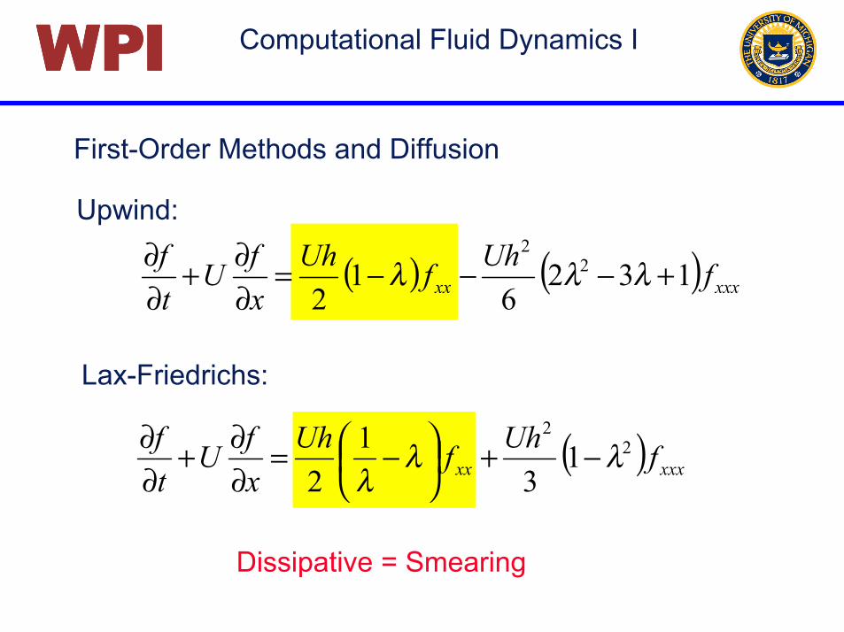
Computational Fluid Dynamics IPPPPIIIIWWWWFirst-Order Methods and Diffusion
Upwind:
( ) ( ) xxxxx fUhfUhxfU
tf 132
61
22
2
+−−−=∂∂+
∂∂ λλλ
Lax-Friedrichs:
( ) xxxxx fUhfUhxfU
tf 2
2
13
12
λλλ
−+
−=
∂∂+
∂∂
Dissipative = Smearing

Computational Fluid Dynamics IPPPPIIIIWWWWSecond-Order Methods and Dispersion
Lax-Wendroff:
( ) ( ) xxxxxxx fUhfUhxfU
tf 2
32
2
18
12
λλλ −−−−=∂∂+
∂∂
Beam-Warming:
( )( ) ( ) ( ) xxxxxxx fUhfUhxfU
tf λλλλ −−−−−=
∂∂+
∂∂ 21
821
62
32
Dispersive = Wiggles

Computational Fluid Dynamics IPPPPIIIIWWWW
Observation 1:Second-order methods tends to capture shaper solution (better accuracy), but they produce wiggly solutions.
Observation 2:First-order methods are dissipative and less accurate, but the solution does not oscillate. (preserves monotonicity).
Computational Fluid Dynamics IPPPPIIIIWWWW
Question: How can we avoid oscillatory behavior ?
(How can we achieve monotone behavior ?)
Godunov Theorem (1959):
“Monotone behavior of a numerical solution cannot be assured for finite-difference methods with more thanfirst-order accuracy.”

Computational Fluid Dynamics IPPPPIIIIWWWW Godunov Theorem - 1
0=∂∂+
∂∂
xfU
tf
For linear equation
which yields:2
22
2
2
;x
fUtf
xfU
tf
∂∂=
∂∂
∂∂−=
∂∂
A general linear scheme can be written as:
∑ ++ =
k
nkjk
nj fcf 1
Expanding in Taylor series aroundnkjf +
njf
)(2
32
222
hOx
fhkxfkhff n
jn
kj +∂∂+
∂∂+=+
Computational Fluid Dynamics IPPPPIIIIWWWW Godunov Theorem - 2
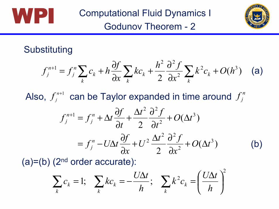
Substituting
Also, can be Taylor expanded in time around
∑ ∑∑ +∂∂+
∂∂+=+
k kk
kkk
nj
nj hOck
xfhkc
xfhcff )(
232
2
221
(a)=(b) (2nd order accurate):2
2;;1
∆=∆−== ∑∑∑ h
tUckh
tUkcck
kk
kk
k
1+njf n
jf
)(2
32
221 tO
tft
tftff n
jnj ∆+
∂∂∆+
∂∂∆+=+
)(2
32
222 tO
xftU
xftUf n
j ∆+∂∂∆+
∂∂∆−=
(a)
(b)
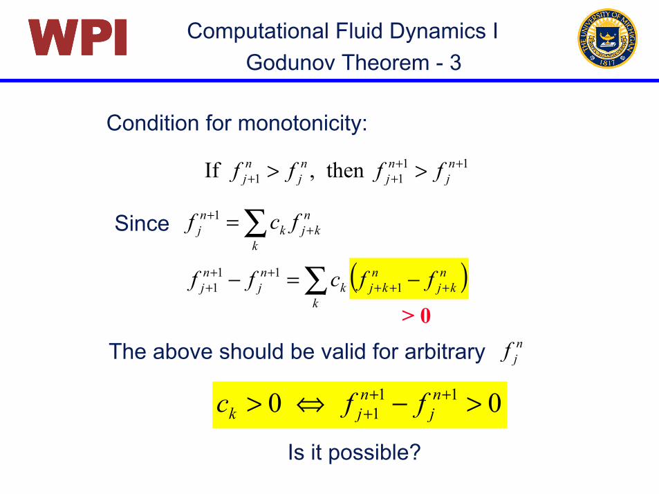
Computational Fluid Dynamics IPPPPIIIIWWWW Godunov Theorem - 3
Condition for monotonicity:11
11 then,If ++++ >> n
jnj
nj
nj ffff
Since ∑ ++ =
k
nkjk
nj fcf 1
( )∑ +++++
+ −=−k
nkj
nkjk
nj
nj ffcff 1
111
> 0The above should be valid for arbitrary
00 111 >−⇔> +++
nj
njk ffc
njf
Is it possible?

Computational Fluid Dynamics IPPPPIIIIWWWW Godunov Theorem - 4
Hence we get:
22;;1
∆=∆−== ∑∑∑ h
tUckh
tUkcck
kk
kk
k
22
=
∑∑∑
kk
kk
kk kcckc
22222
=
∑∑∑
kk
kk
kk keeke
Define: )0(2 >= kkk cec
This violates Cauchy inequality ( )( ) ( )2babbaa ⋅≥⋅⋅
Monotone 2nd Order scheme is impossible!

Computational Fluid Dynamics IPPPPIIIIWWWW Godunov Theorem - 5
The Godunov theorem suggests that monotone schemes are limited to the first order schemes.
However, Godunov theorem is valid only for linear schemes.
The Godunov theorem can be circumvented by nonlinear schemes, even for linear equations.
⇒ Basis for higher-order monotone schemes(TVD, higher-order upwind)
Computational Fluid Dynamics IPPPPIIIIWWWW
In the following, we will discuss various approaches to achieve monotone solution for Euler equations:
- Flux-splitting- Artificial viscosity- Godunov method- Higher-order upwind and TVD
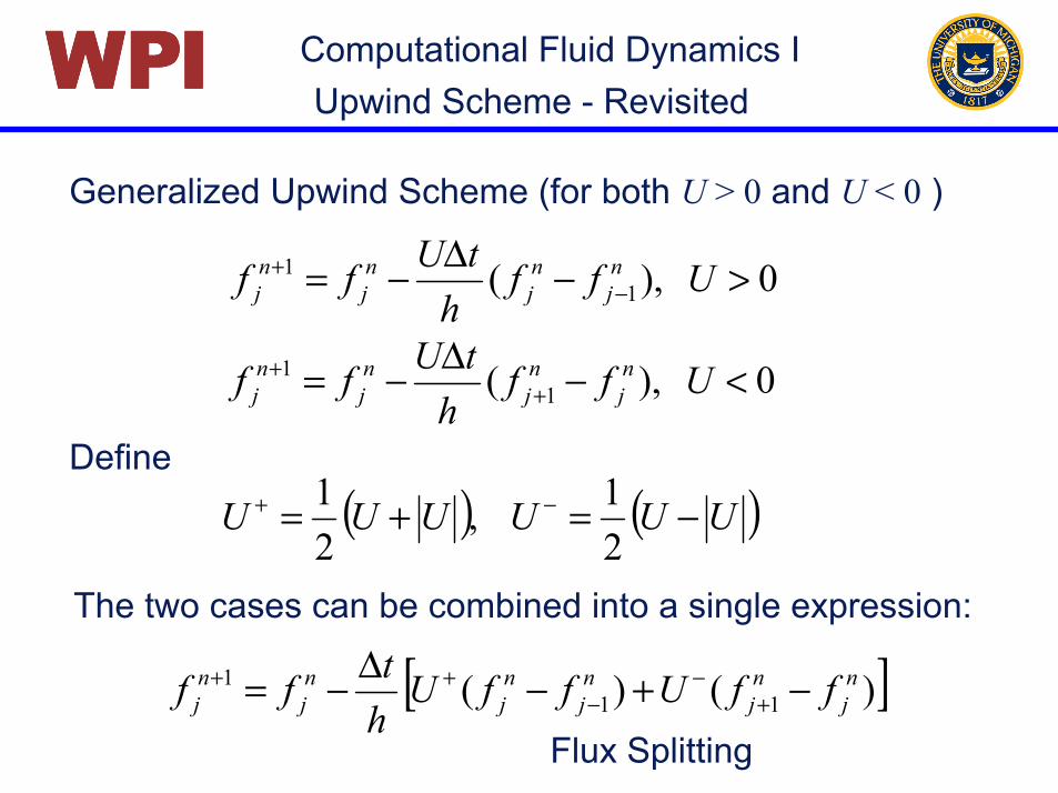
Computational Fluid Dynamics IPPPPIIIIWWWWGeneralized Upwind Scheme (for both U > 0 and U < 0 )
0),( 11 >−∆−= −+ Uff
htUff n
jnj
nj
nj
0),( 11 <−∆−= ++ Uff
htUff n
jnj
nj
nj
Define( ) ( )UUUUUU −=+= −+
21,
21
The two cases can be combined into a single expression:
[ ])()( 111 n
jnj
nj
nj
nj
nj ffUffU
htff −+−∆−= +
−−
++
Upwind Scheme - Revisited
Flux Splitting

Computational Fluid Dynamics IPPPPIIIIWWWW
Or, substituting
Recall Lax-Wendroff
)2(2
)(2 1111
1 nj
nj
nj
nj
nj
nj
nj fff
htU
ffhtUff −+−+
+ +−∆
+−∆−=
−+ UU ,
central difference + artificial viscosity
( ) ( )nj
nj
nj
nj
nj
nj
nj fff
htUff
htUff 112
22
111 2
22 −+−++ +−∆+−∆−=
Upwind Scheme - Revisited

Computational Fluid Dynamics IPPPPIIIIWWWW
Two options for hyperbolic equations:
1. Use directionally-biased upwind scheme(Flux splitting)
2. Use central differencing and introduce numericalviscosity (Artificial viscosity)
Upwind Scheme - Revisited
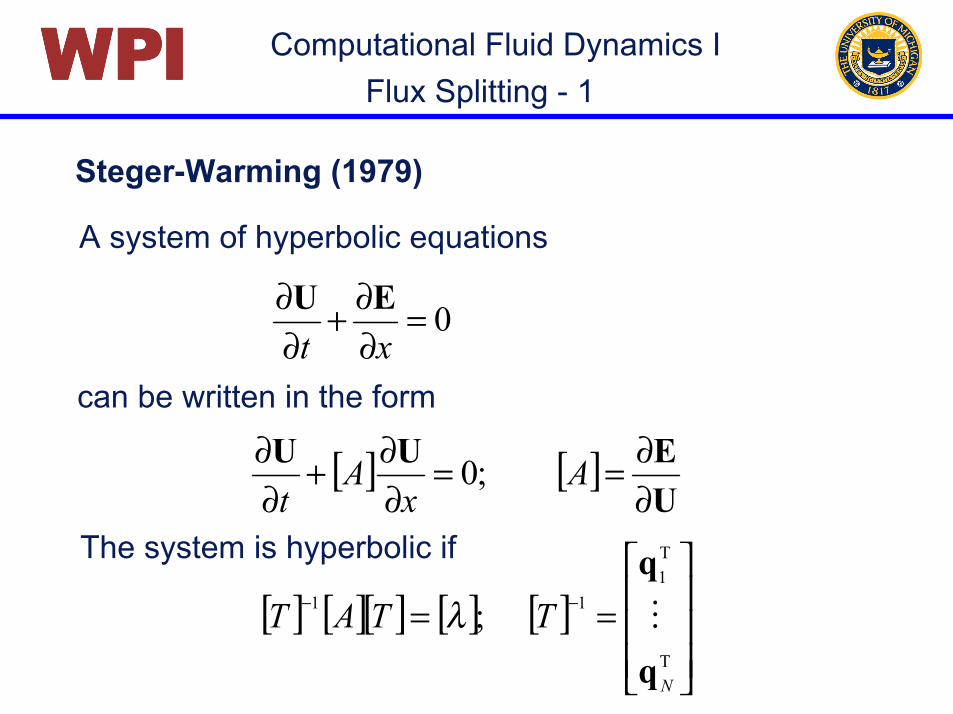
Computational Fluid Dynamics IPPPPIIIIWWWWSteger-Warming (1979)
A system of hyperbolic equations
Flux Splitting - 1
0=∂∂+
∂∂
xtEU
can be written in the form
[ ] [ ]UEUU∂∂==
∂∂+
∂∂ A
xA
t;0
The system is hyperbolic if
[ ] [ ][ ] [ ] [ ]
== −−
T
T1
11 ;
N
TTATq
q!λ

Computational Fluid Dynamics IPPPPIIIIWWWWFlux Splitting - 2
[ ] [ ][ ][ ] UUE 1−== TTA λ
The matrix of eigenvalues is divided into two matrices
[ ] [ ] [ ] [ ][ ][ ] [ ][ ][ ] 11 −−−+−+ +=+= TTTTAAA λλHence
[ ]λ[ ] [ ] [ ]−+ += λλλ
Define −+ += EEE [ ] [ ]( )UEUE −−++ == AA ,
Conservation law becomes
0=∂∂+
∂∂+
∂∂ −+
xxtEEU
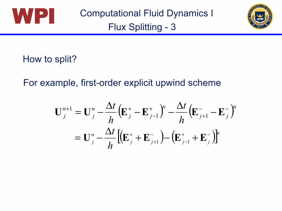
Computational Fluid Dynamics IPPPPIIIIWWWWFlux Splitting - 3
For example, first-order explicit upwind scheme
( ) ( )njjn
jjnj
nj h
tht −−
++−
++ −∆−−∆−= EEEEUU 111
How to split?
( ) ( )[ ]njjjjnj h
t −+−
−+
+ +−+∆−= EEEEU 11

Computational Fluid Dynamics IPPPPIIIIWWWWFlux Splitting - 4
Example: 1-D Hyperbolic Equation
02
22
2
2
=∂∂−
∂∂
xfc
tf
xfw
tfv
∂∂=
∂∂= ;0
010 2
=
−
−+
x
x
t
t
wvc
wv
Leading to
[ ]
−
−=
∂∂=
−−
=
=
010
;;22 c
Av
wcwv
UEEU
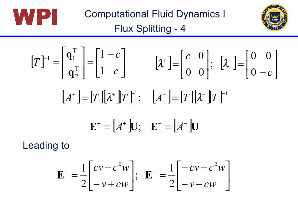
Computational Fluid Dynamics IPPPPIIIIWWWWFlux Splitting - 4
Leading to
[ ]
−=
=−
cc
T11
T2
T11
qq [ ] [ ]
−
=
= −+
cc
000
;000
λλ
−−−−
=
+−−
= −+
cwvwccv
cwvwccv 22
21;
21 EE
[ ] [ ][ ][ ] [ ] [ ][ ][ ] 11; −−−−++ == TTATTA λλ
[ ] [ ]UEUE −−++ == AA ;
Computational Fluid Dynamics IPPPPIIIIWWWWArtificial Viscosity [Ref: Hirsch, vol. 2, Ch. 17]
The centered difference method (e.g. Lax-Wendroff) - Second order accuracy- Oscillation near discontinuity
In order to “damp out” oscillation, we can either- Use implicit numerical viscosity (upwind) or- Add an explicit numerical viscosity
Artificial Viscosity - 1

Computational Fluid Dynamics IPPPPIIIIWWWWVon Neumann and Richtmyer (1950)
0=∂∂+
∂∂
xF
tf
xfDh
xfFF
∂∂=
∂∂−=′ 2; αα
- Simulates the effect of the physical viscosity on thegrid scale, concentrated around discontinuity and negligible elsewhere.
- h2 is necessary to keep the viscous term of higher order.
Artificial Viscosity - 2
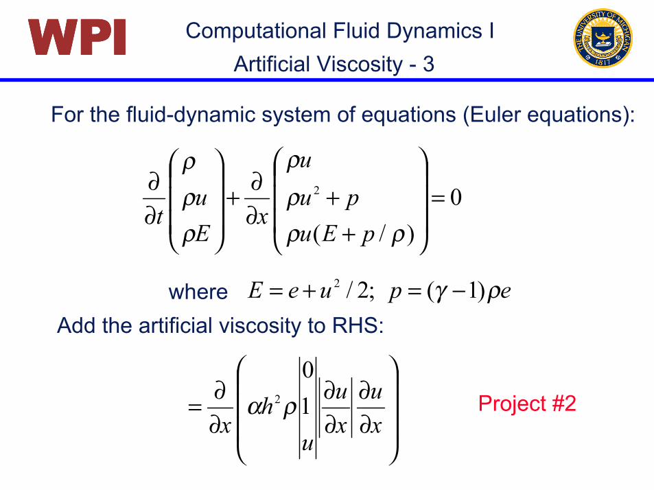
Computational Fluid Dynamics IPPPPIIIIWWWWFor the fluid-dynamic system of equations (Euler equations):
0)/(
2 =
++
∂∂+
∂∂
ρρρρ
ρρρ
pEupu
u
xEu
t
epueE ργ )1(;2/2 −=+=Add the artificial viscosity to RHS:
where
∂∂
∂∂
∂∂=
xu
xu
uh
x10
2ρα Project #2
Artificial Viscosity - 3
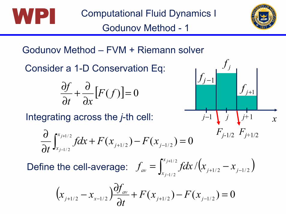
Computational Fluid Dynamics IPPPPIIIIWWWWGodunov Method – FVM + Riemann solver
[ ] 0)( =∂∂+
∂∂ fF
xtf
Consider a 1-D Conservation Eq:
Integrating across the j-th cell:
Godunov Method - 1
Fj-1/2 Fj+1/2
1+jff j−1
jf
xj j+1j−1
0)()( 2/12/1
2/1
2/1=−+
∂∂
−+∫+
−jj
x
xxFxFfdx
tj
j
Define the cell-average: ( )2/12/1/2/1
2/1−+ −= ∫
+
−jj
x
xav xxfdxf j
j
( ) 0)()( 2/12/12/12/1 =−+∂∂− −+−+ jj
avxj xFxF
tfxx

Computational Fluid Dynamics IPPPPIIIIWWWWFor simplicity, assuming uniform grid,
Integrating in time by
where the time integration is done by solving Riemann Problem for each cell boundary:
Godunov Method - 2
∆−
∆∆−= ∫ ∫
∆+ ∆+
−++
tt
t
tt
t jjn
avn
av dtFt
dtFth
tff 2/12/11 11
hxx xj =− −+ 2/12/1
t∆
[ ] 0)( =∂∂+
∂∂ fF
xtf
>≤
=++
+
2/11
2/1)0,(jj
jj
xxfxxf
xf 1+jfjf
xj j+1
t
2/1+= jcdtdx
t+∆t

Computational Fluid Dynamics IPPPPIIIIWWWWWave Diagram:
Godunov Method - 3
1+jff j−1jf
j j+1j−1
ShockShockRarefaction
Wave
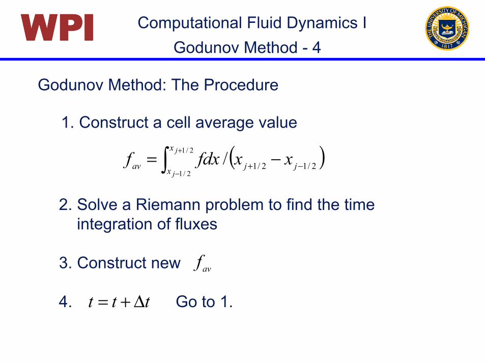
Computational Fluid Dynamics IPPPPIIIIWWWWGodunov Method: The Procedure
Godunov Method - 4
1. Construct a cell average value
( )2/12/1/2/1
2/1−+ −= ∫
+
−jj
x
xav xxfdxf j
j
2. Solve a Riemann problem to find the time integration of fluxes
3. Construct new
4. Go to 1.
avf
ttt ∆+=

Computational Fluid Dynamics IPPPPIIIIWWWWExample: Inviscid Burgers Equation
Godunov Method - 5
021 2 =
∂∂+
∂∂ f
xtf
>≤
=++
+
2/11
2/1)0,(jj
jj
xxfxxf
xf
Initial Condition:
Characteristic Velocity:
21
2/12/1
+
++
+=
= jj
jj
ffdtdxc

Computational Fluid Dynamics IPPPPIIIIWWWWThe Formula:
Godunov Method - 6
1+> jj ff
><
=++
+
2/11
2/1
//
jj
jj
ctxfctxf
f
Shock waves
Expansion Waves
( ) 2/12/1 ++ += jjj ffc
<
>=
++
+
+ 0
0
2/12
121
2/12
21
2/1
jj
jj
j cf
cfF
1+< jj ff
><<
<=
++
+
+
2/11
1
2/1
///
/
jj
jj
jj
ftxfftxftx
ftxff
<<<
>>>
<<
=
+++
++
+
+
00
00
00
12/12
121
12/12
21
1
2/1
jjjj
jjjj
jj
j
ffcf
ffcf
ff
F
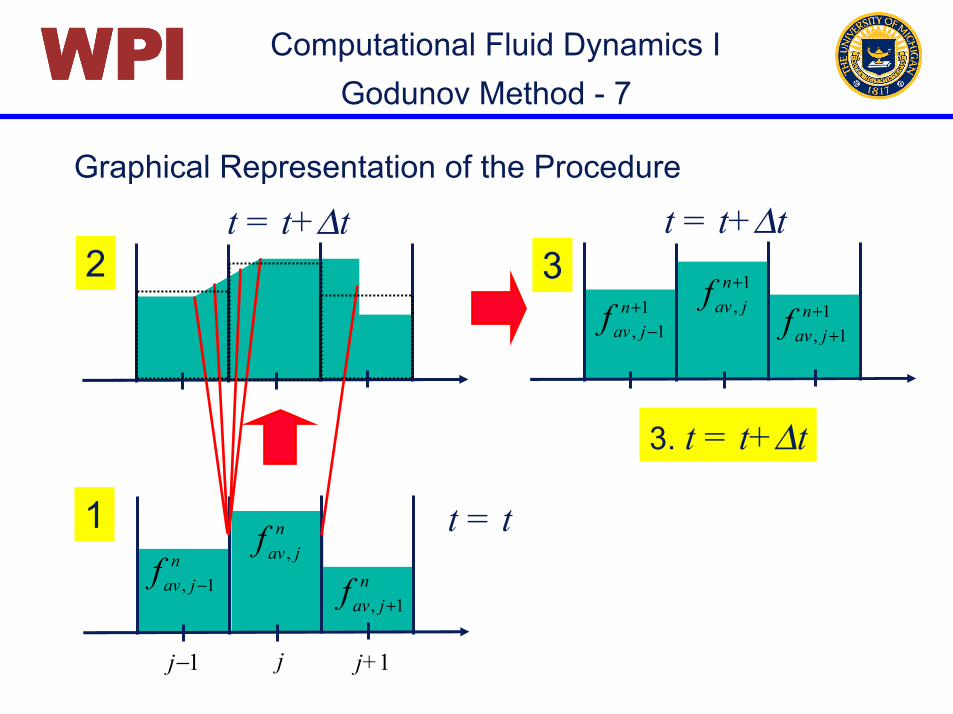
Computational Fluid Dynamics IPPPPIIIIWWWWGraphical Representation of the Procedure
Godunov Method - 7
njavf 1, +
njavf 1, −
njavf ,
j j+1j−1
2
3. t = t+∆t
1,+n
javf1
1,++
njavf1
1,+−
njavf
t = t+∆t
1
t = t+∆t3
t = t

Computational Fluid Dynamics IPPPPIIIIWWWW
Godunov method implicitly assumes that the waves fromadjacent cells do not interact.
⇒ The wave can travel at most half cell in distance during one time step
Godunov Method - 8
21
max ≤∆htf
Stability Condition
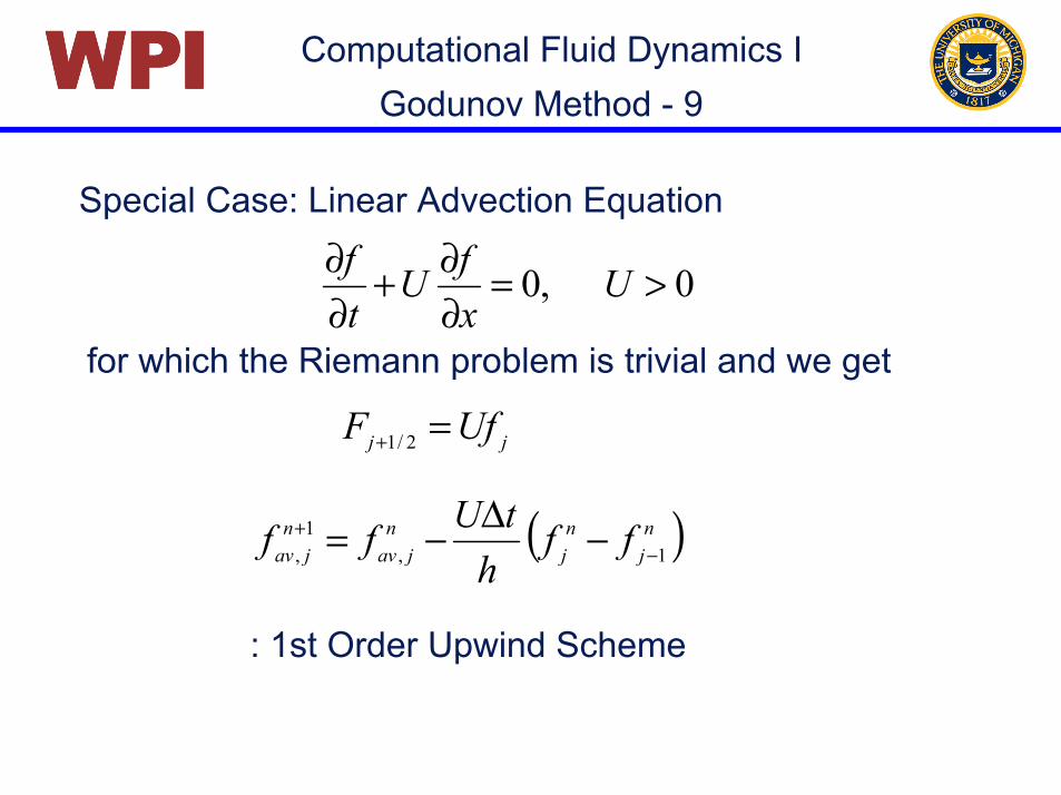
Computational Fluid Dynamics IPPPPIIIIWWWWSpecial Case: Linear Advection Equation
Godunov Method - 9
0,0 >=∂∂+
∂∂ U
xfU
tf
for which the Riemann problem is trivial and we get
( )nj
nj
njav
njav ff
htUff 1,
1, −+ −∆−=
jj UfF =+ 2/1
: 1st Order Upwind Scheme

Computational Fluid Dynamics IPPPPIIIIWWWWFor general nonlinear problems, the Riemann problemrequires nonlinear iterations and becomes expensive.
Godunov Method - 10
Approximate Riemann Solver : Flux determined from local conditions.
- Roe Scheme: allows expansion shock (nonphysical)
- Enquist-Osher scheme: removing expansion shock(entropy condition)
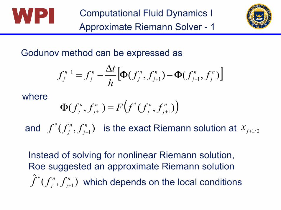
Computational Fluid Dynamics IPPPPIIIIWWWWGodunov method can be expressed as
Approximate Riemann Solver - 1
where
[ ]),(),( 111 n
jnj
nj
nj
nj
nj ffff
htff −+
+ Φ−Φ∆−=
( )),(),( 1*
1nj
nj
nj
nj fffFff ++ =Φ
and is the exact Riemann solution at ),( 1* n
jnj fff + 2/1+jx
Instead of solving for nonlinear Riemann solution,Roe suggested an approximate Riemann solution
),(ˆ1
* nj
nj fff + which depends on the local conditions
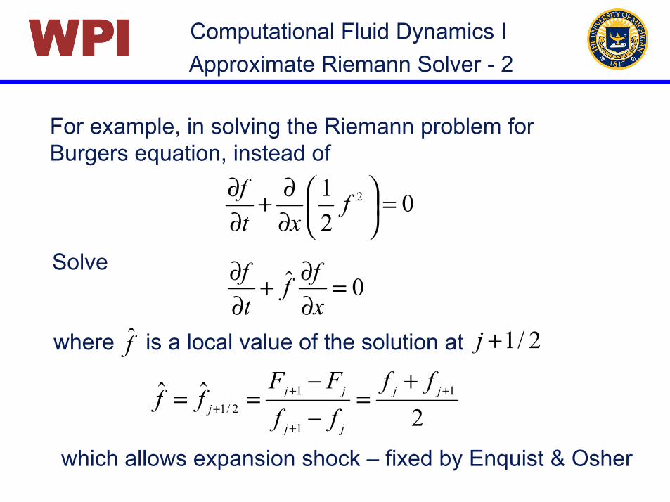
Computational Fluid Dynamics IPPPPIIIIWWWWFor example, in solving the Riemann problem for Burgers equation, instead of
Approximate Riemann Solver - 2
Solve
021 2 =
∂∂+
∂∂ f
xtf
where is a local value of the solution at
2ˆˆ 1
1
12/1
+
+
++
+=
−−
== jj
jj
jjj
ffffFF
ff
0ˆ =∂∂+
∂∂
xff
tf
f̂ 2/1+j
which allows expansion shock – fixed by Enquist & Osher
Computational Fluid Dynamics IPPPPIIIIWWWWHigher Order Upwind Method:
MUSCL (Monotone Upstream-centered Schemesfor Conservation Laws) - Van Leer (1979)
Higher Order Upwind
Godunov method starts from the cell average values,and solve Riemann problem.
To increase the order of accuracy, construct a piecewiselinear approximation within in each cell in determining theflux terms.
Coupled with approximate Riemann solver.
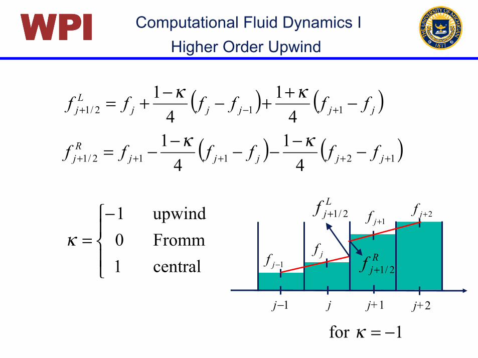
Computational Fluid Dynamics IPPPPIIIIWWWWHigher Order Upwind
j j+1j−1 j+2
1+jf 2+jf
jf1−jf
Ljf 2/1+
Rjf 2/1+
( ) ( )jjjjjLj ffffff −++−−+= +−+ 112/1 4
14
1 κκ
( ) ( )12112/1 41
41
+++++ −−−−−−= jjjjjRj ffffff κκ
−
=central1Fromm0upwind1
κ
1for −=κ
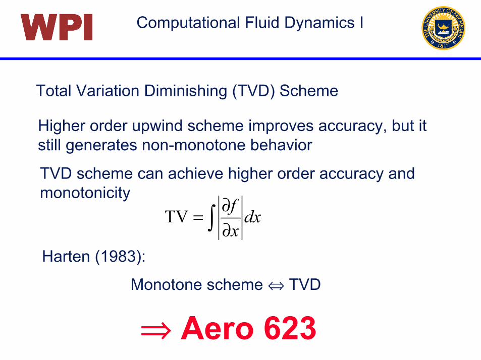
Computational Fluid Dynamics IPPPPIIIIWWWWTotal Variation Diminishing (TVD) Scheme
Higher order upwind scheme improves accuracy, but itstill generates non-monotone behavior
TVD scheme can achieve higher order accuracy and monotonicity
∫ ∂∂= dx
xfTV
Harten (1983):
Monotone scheme ⇔ TVD
⇒⇒⇒⇒ Aero 623


![[PPT]Computational Fluid Dynamics: An Introductionuser.engineering.uiowa.edu/~fluids/posting/home/CFD/CFD... · Web viewIntroduction to Computational Fluid Dynamics (CFD) Maysam Mousaviraad,](https://img.pdfslide.us/doc/110x75/5aedbf837f8b9a90319017cb/pptcomputational-fluid-dynamics-an-fluidspostinghomecfdcfdweb-viewintroduction.jpg)