wp_chap5

7/29/2019 wp_chap5

http://slidepdf.com/reader/full/wpchap5 1/15

1.138J/2.062J/18.376J, WAVE PROPAGATION

Fall, 2004 MIT Notes by C. C. Mei CHAPTER FIVE

MULTIPLE SCATTERING BY AN EXTENDED REGION OF

INHOMOGENEITIES

1 Bragg scattering in a periodic medium

Longshore sand bars are often found along gentle beaches. The number of bars can range from a few to dozens and the spacing from tens to hundreds of meters. The bar amplitudes can be as high as a meter. Figure 1 shows a sample profile in Chesapeake Bay, Maryland, USA, recorded by accoustic sounding (Dolan, 1982).

Scientifically it is natural to ask how these sand bars are generated and how the bars affect the propagation of waves. In fact these two questions are coupled through the complex dynamics of sediment transport. It is easier to just consider the second question.

If the bar amplitudes are small, D h, one might expect their effects on a train of

progresseive

waves

to

be

small

and

apply

a straightforward

second-order

analysis

so

that the effect on waves will appear at the order kA(KD). The situation is different if however the incident waves are twice as long as the bar spacing, i.e., K = 2k then the phenomenon of Bragg resonance occurs and the reflection by many small and pe-

riodic bars can be very strong. The source of this resonance is due to constructive interference of incident and reflected waves and is well known in x-ray diffraction by crystaline materials. Referring to Fig. 2 where a number of bars of wavelength λb are fixed on a horizontal bed, we consider the propagation of a train of waves incident from the left. Every wave crest passing over a bar will be mostly transmitted toward the next bar ahead and sends a weak reflected wave towards the bar behind. At any given bar crest, say B, the total amplitude of the left-going wave is the sum of all left-going wave crests each of which is the consequence of reflection by the nth bar on the right. Therefore each of these crests has traveled the distance of 2nλb. When

1

7/29/2019 wp_chap5


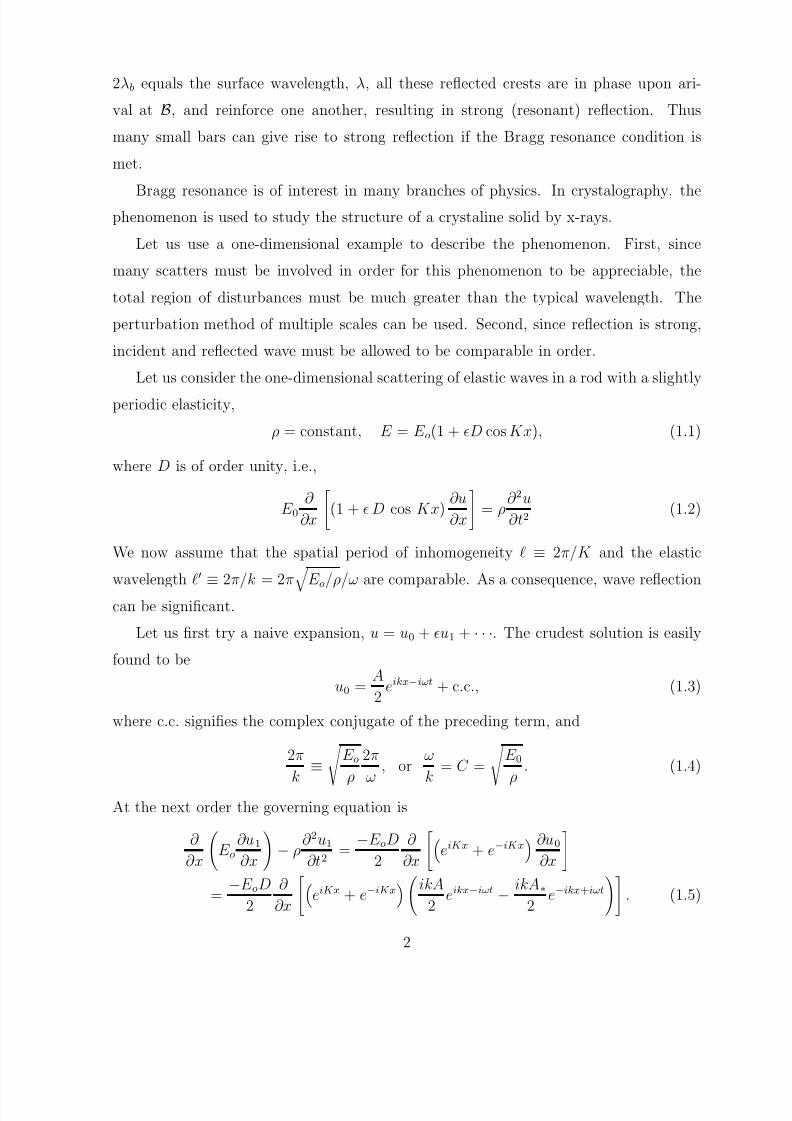
2λb equals the surface wavelength, λ, all these reflected crests are in phase upon ari-

val at B, and reinforce one another, resulting in strong (resonant) reflection. Thus many small bars can give rise to strong reflection if the Bragg resonance condition is met.

Bragg resonance

is

of

interest

in

many

branches

of

physics.

In

crystalography,

the

phenomenon is used to study the structure of a crystaline solid by x-rays.

Let us use a one-dimensional example to describe the phenomenon. First, since many scatters must be involved in order for this phenomenon to be appreciable, the total region of disturbances must be much greater than the typical wavelength. The perturbation method of multiple scales can be used. Second, since reflection is strong, incident and reflected wave must be allowed to be comparable in order.

Let us consider the one-dimensional scattering of elastic waves in a rod with a slightly periodic elasticity,

ρ = constant, E = E o(1 + D cos Kx), (1.1) where D is of order unity, i.e.,

∂ ∂u ∂ 2 u E 0 (1 + D cos Kx) = ρ (1.2)

∂x ∂x ∂t2

We now assume that the spatial period of inhomogeneity ≡ 2π/K and the elastic wavelength ≡ 2π/k = 2π E

o/ρ/ω are comparable. As a consequence, wave reflection

can be significant. Let us first try a naive expansion, u = u0 + u1 + · · ·. The crudest solution is easily

found to be A ikx−iωt u0 = e + c.c., (1.3)2

where c.c. signifies the complex conjugate of the preceding term, and 2π E o 2π ω E 0

≡ , or = C = . (1.4)k ρ ω k ρ

At the next order the governing equation is ∂u0∂ ∂u1 ∂ 2u1 −E oD ∂ iK x −iK x E o − ρ = e + e

∂x ∂x ∂t2 2 ∂x ∂x ikA −E oD ∂ e iK x + e −iK x e ikx−iωt − ikA∗ −ikx+iωt . (1.5)= e

2 ∂x 2 2 2

7/29/2019 wp_chap5


Clearly, whenK = 2k + δ, δ k, (1.6)

some of the forcing terms on the right will be close to a natural mode exp(±i(kx + ωt)). Resonance of the reflected waves must be expected. It sufices to illustrate the response to one of these terms,

E ∂ 2u1

o − ρ∂ 2u1

= Aeiφoe ıδx , with φo = kx + ωt. ∂x2 ∂t2

Combining homogeneous and inhomogeneous solutions and requiring that u1(0, t) = 0, we find

uAeiφo 1 − eiδx

1 = . E o((k + δ)2 − k2)

Clearly if δ = O(), u1 ∼ O(/δ) and is not small compared to u0 except for δx 1. Furthermore as x increases, u1 grows as x. This implies that the reflected waves are resonated and is no longer much smaller that the incident waves in the distance x = O(1). The relation 2K = k (cf. (1.6) is the well-known condition for Bragg resonance.

Let us now focus attention on the case of Bragg resonance. To render the solution uniformly valid for all x, we introduce fast and slow variables in space

x, x = x (1.7) To allow slight detuning from exact resonance, we assume that the incident wave fre-

quency is ω + ω, where ω represents the small detuning and gives rise to a very slow variation in time. Therefore two time variables are needed,

t, t = t (1.8) The following multiple scale expansion is then proposed,

x; t, t) + u1(x, ¯u = u0(x, ¯ x; t, t) + · · · . (1.9) After making the changes

∂ ∂ ∂ ∂ ∂ ∂ → + , → +

x∂x ∂x ∂ ∂t ∂t ∂t(1.10)

3

7/29/2019 wp_chap5


and substituting (1.9), (1.10) into (1.2), we get∂ ∂u0 ∂ 2 u0

E o − ρ = 0 (1.11)∂x ∂x ∂t2

at O(1). Anticipating strong but finite reflection, we take the solution to be A B u0 = e ikx−iωt + ∗ + e −ikx−iωt + c.c.. (1.12)2 2

where A(x1, t1) and B(x1, t1) vary slowly in space and time. At the order O() we have ∂ ∂u1 ∂ 2u1 ∂ 2u0 ∂ 2u0

E o − ρ = −2E o + 2ρ x∂x ∂x ∂t2 ∂x∂ ∂t∂t ∂u0−2ikx − E oD ∂

e 2ikx + e 2 ∂x ∂x

∂A (ik)e ikx−iωt ∂B

(−ik)e −ikx−iωt = −E o + c.c. + + c.c. ∂ ∂ x x

∂B (−iω)e −ikx−iωt +ρ ∂A

(−iω)e ikx−iωt + c.c. + + c.c. ∂t ∂t ∂

2ikx − E oD ∂ e + c.c. Aeikx−iωt + c.c. + Be−ikx−iωt + c.c. (1.13)

4 ∂x ∂x The last line can be reduced to

− E oDk2Beikx−iωt + c.c. + k2Ae−ikx−iωt + c.c.

4 −3k

2

Ae

3ikx−iωt + c.c.

−

3k

2

Be

−3ikx−iωt + c.c.

To avoid unbounded resonance of u1, i.e., to ensure the solvability of u1, we equate to zero the coefficients of terms e±i(kx−ωt) and e±i(kx+ωt) on the right of (1.13). The following equations are then obtained:

∂A ∂A ikCD ∂t

+ c∂

= 4 B (1.14)

x ∂B ∂B ikCD ∂t

− c∂

= 4 A, (1.15)

x where E o/ρo = C = ω/k denotes the phase speed. These equations govern the macroscale variation of the envelopes of the incident and reflected waves, and can be combined to give the Klein-Gordon equation

∂ 2A ∂ 2 A kC D 2 − C 2 + A = 0. (1.16)

∂ 2∂t2 x 4 4

7/29/2019 wp_chap5


Note that kC D ωD

4 = 4 ≡ Ω0 (1.17)

has the dimension of frequency. With suitable initial and boundary conditions on the macro scale, one finds the slow

variation of these wave envelopes, hence the global behaviour of wave motion. Let the inhomogeneity of wavenumber 2k be confined in 0 < x < L and the incident

wave train be slightly detuned from resonance, so that the wave frequency is ω + Ω and the wavenumber is k + K , where Ω = O(ω) and K = O(k). Since ω + Ω and k + K must be related by the dispersion relation (1.4),

Ω = KC . (1.18) The detuned incident wave

ζ = Ao exp[i(k + K )x − (ω + Ω)t] + ∗ , x < 0 , (1.19)¯

can be alternatively written as x, t)e ikx−iωt ¯ζ = A(¯ ¯ , x < 0 , (1.20)

where x−Ct)x, t) = Aoe iK (¯ , x < 0 . (1.21)A(¯ ¯ ¯

When such a wavetrain passes a patch of periodic bars, A and B must vary with x and t according to (1.14) and (1.15).

To the left and to the right of the bars, the governing equations are simply ¯ ¯At + CAx = 0 , Bt − CBx = 0 , x < 0 , and x > L . (1.22)¯ ¯

We shall assume further that B = 0 for x > L. Over the bars (1.14) and (1.15), or (1.16) hold. In order that displacement and stress and horizontal velocity be continuous at x = 0, L, A and B must be continuous at x = 0, L. Since the solutions must be of the form,

x), R(¯ x < L . (A, B) = A0(T (¯ x))e −iΩt , 0 < ¯

T and R are governed by (Ω2 − Ω2

0)T x¯ + T = 0 , 0 < x < L . ¯x

C 5

7/29/2019 wp_chap5


Several cases can be distinguished according to the sign of Ω2 − Ω2 0:

Subcritical detuning : 0 < Ω < Ω0 . Let

− Ω2)1/2Qc = (Ω2 (1.23)0

then

iQC cosh Q(L − ¯ x)x) + Ω sinh Q(L − ¯T (x) = (1.24)

iQC cosh QL + Ω sinh QL and

Q sinh Q(L − x)R(x) = . (1.25)

iQC cosh QL + Ω sinh QL On the incidence side the reflection coefficient is just R(0) and on the transmission side the transmission coefficient is T (L). Clearly the dependence on L and x is monotonic. ¯

In the limit of L → ∞, it is easy to find that x xT (x) = e −Q¯ , R(x) = Q

e −Q¯ . (1.26)iQC + Ω

Thus all waves are localized in the range x < O(1/Q). Supercritical detuning : Ω > Ω0 .

Let P c = (Ω2 − Ω2

0)1/2 (1.27) then the transmission and reflection coifficients are:

P C cos P (L − ¯ x)x) − iΩsin P (L − ¯T (x) = (1.28)

P C cos P L − iΩsin P L and

−iQ0 sin P (L − x)R(x) = . (1.29)

P C cos P L − iΩsin P L The dependence on L and x is clearly oscillatory. Thus Ω0 is the cut-off frequency mark-

ing the transition of the spatial variation. For subcritical detuning complete reflection can occur for sufficinetly large L. For super-critical detuning there can be windows of strong transission.

In the special case of perfect resonance, we get from (1.24) and (1.25) that x)A cosh Ωo(L−¯ B i sinh Ωo(L−x)

x) = Ao =

cosh ΩoL R(¯ C T (¯ C x) = Ao = −

cosh ΩoL . (1.30) C C

6

7/29/2019 wp_chap5


In a laboratory experiment for water waves, Heathershaw(1982) installed 10 sinu-

soidal bars of amplitude D = 5 cm and wavelength 100 cm on the bottom of a long wave flume. Incident waves of length 2π/k = 200 cm were sent from one side of the bar patch. On the transmission side, waves are essentially absorbved by breaking on a gentle

beach.

Sizable

reflection

coefficients

were

measured

along

many

stations

over

the bar patch. This experiment gives the first observed evidence of strong reflection by periodic bars. Let us apply the present theory to a more general case where the normally incident wave is slightly detuned from perfect resonance.

Clearly they both decrease monotonically from ¯ x = L. These results agree x = 0 to quite well with the experiments of Heathershaw, as shown in Fig. 3, therefore confirm that enough small bars can generate strong reflection, especially in very shallow water. Exercise

5.1:

Bragg

resonance

by

a

corrugated

river

bank .

An infinitely long river has contant depth h and contant averaged width 2a. In the

stretch 0 < x < L, the banks are slightly sinusoidal about the mean so that y = ±a ± B sin Kx , KB ≡ 1 . (1.31)

See Fig. 4. Let a train of monochromatic waves be incident from x ∼ −∞, ζ = A

e i(kx−ωt) (1.32)2

where kh, ka = O(1). Develop a uniformly valid linearized theory to predict Bragg resonance. Can the corrugated boundary be used to reflect waves as a breakwater? Discuss your results for various parameters that can affect the function as a breakwater.

2 Wave localization in a random medium

[Ref]: Mei & Pihl Localization of nonlinear dispersive waves in weakly random media, Proc. Roy. Soc. Lond. 2002, 458, 119-134.

There are numerous situations where one needs to know how waves propagate through a medium with random impurities: light through sky with dust particles, sound through water with bubbles, elastic waves through a solid with cracks, fibers, cavities, hard or soft grains. Sea waves over a irregular topography, etc. It is known that, for one-dimensional

7

7/29/2019 wp_chap5


propagation, multiple scattering yields a change in the wavenumber (or phase velocity) as well as an amplitude attenuation, if the inhomogeneities extend over a large distance. These changes amount to a shift of the complex propagation constant with the real part corresponding to the wavenumber and the imaginary part to attenuation. In particular, the

spatial

attenuation

is

a distinctive

feature

of

randomness

and

is

effective

for

a broad

range of incident wave frequencies.This is in sharp contrast to periodic inhomogeneities which cause strong scattering only for certain frequency bands (Bragg scattering, see e.g., Chapter 1). Phillip W. Anderson (1958) was the first to show, in the context of solid-state physics, that a metal conductor can behave like an insulator, if the ,ir-

crostructure has is disordered. This phenomoena, now called Anderson localization , is now known to be important in classical systems also. A survey of localization in many types of classical waves based on linearized theories can be found in Sheng (1998).

For weak inhomogeneties, the shift of propagation constant amounts to slow spatial modulations with a length scale much longer than the wavelnegth by a factor inversely proportional to the correlation of the fluctuations. In this section we apply the method of multiple scales to introduce the theory for the simplest exampole of one-dimensional sound.

We begin with the Helmhotz equation for sinusoidal waves, d2U

+ k2(1 + V (x))2U = 0, ∞x < ∞. (2.1)dx2

Let V (x) be a random function of x with zero mean and V (x) → 0, for x ∼ −∞. An incident wave train

U inc = A0e ikx (2.2) arrives from the left-infinity where there is no disorder. What will happen, on the average, to waves after they enter the region of disorder?

Consider an ensemble of random media. For each realization, the wave number now fluctuates about the mean k by the amount order O(). Since V = 0, we expect that, on the average, the wave phase is affected only by the root-mean-square, wich is of the order O(2). With this guess, it is natural that slow variations described by x2 = 2x will be relevant. We assume that the disorder has two characteristc scales so that

V = V (x, x2) (2.3) 8

7/29/2019 wp_chap5


For simplicity we shall further assume that V is stationary with respect to the short scale

V (x, x2)V (x , x2) = C vv (|x − x |, x2) (2.4) where f denotes the ensemble average of f .

Let us try the following expansion, U = U 0(x, x2) + U 1(x, x2) + 2U 2(x, x2) + · · · (2.5)

Subsituting (2.5) into (2.1), the following perturbation equations are found, ∂ 2 U 0

+ k2U 0 = 0, (2.6)∂x2

∂ 2U 1 + k2U 1 = −2k2V U 0, (2.7)

∂x2 ∂ 2 U 2

+ k2U 2 = −2 ∂U 0 − k2 2V U 1 + V 2U 0 , (2.8)

∂x2 ∂x∂x2 The solution at the leading order is

U 0 = A(x2)e ikx where A(0) = Ao. (2.9) At the next order the inomogeneous equation is solved by Green’s function G(x, x)

defined by ∂ 2 G

+ k2

G = δ(x − x ), (2.10)∂x2 where G is outgoing at infinities. The solution is easily found to be

G = − ie ik|x−x| (2.11)

2k (2.12)

The solution for U 1 is

∞ U 1

=

−

dx

G(x, x

) 2k

2

V (x , x2)U (x , x2)

−∞ ∞

ik|x−x|= ik dxV (x , x2)e ikx e (2.13)

−∞ which is random with zero mean. For the O(2) problem, we note that

2 ∂ 2 U 0 = 2ike ikx ∂A

,∂x∂x ∂x2

9

7/29/2019 wp_chap5


ikx ik|x−x| −ik(x−x2k2V U 1 = 2ikA(x2)e V (x, x2)V (x , x2)e e )dx , k2V 2U 0 = k2 e ikxV (x, x2)V (x, x2)A(x2).

We now take the ensemble average of (2.14), and get ∂

2 U 2

∂A

+ k2U 2 = −2ike ikx

∂x2 ∂x2 ∞ ikx ik|x−x| −ik(x−x)dx− 2ikk2A(x2)e V (x, x2)V (x , x2)e e

−∞ − k2 e ikxA(x2)V 2(x, x2)

For U 2 to be solvable, we set the right-hand-side to zero, ∞∂ A + A k2 dxC vv (|x − x |, x2)e ik|x−x|e −ik(x−x)dx − ik

C vv (0, x2) = 0 ∂x2 −∞ 2

Clearly the integral above is just a known function of x2 once the correlation function is prescribed. Denoting

∞β (x2) = β r + iβ i = k2 dxC vv (|x − x |, x2)e ik|x−x|e −ik(x−x)dx − ik

C vv (0, x2). (2.14) −∞ 2

If β = 0, x2 < 0 and β = constant, x2 > 0, then the solution is simply A = A(0)e −iβ rx2e −β ix2 (2.15)

Thus, not only the phase is changed but the amplitude decays exponentially over the distance O(L) where

L = 1/β i2 (2.16)

In summary, due to scattering by disorder, an apparent damping is created. The distance L is called the localization distance.

For simple correlation functions, the integral for β can be explicilty evaluated. For example let

α

C vv (|x − x , x2|) = σ2(x2)e −α|x−x| (2.17) so that σ2 is the RMS amplitude of the disorder. We leave it as an exercise to show that

2 + 2k2 ikσ2 α2 β = β r + iβ i = 2k2σ2 − (2.18)

α(α2 + 4k2) 2 α2 + 4k2

10

7/29/2019 wp_chap5


The leading order wave is 2σ2 α2 22k2σ2 α2 + 2k2

U 0 = A0 exp ik 1 + 2 α2 + 4k2 x exp −

α α2 + 4k2 x , x > 0 (2.19)

As the RMS of the disorder increases, the wwavnumber increases, hence the wave length decreases. A dimensionless localization distance can be defined as

1 1 + 4k2/α2 kLloc = (2.20)

22σ2 (k/α)(1 + 2k2/α2) Note that the correlation length is O(α−1). If the waves are much longer than the correlation length, k/α 1; kLloc increases without bound and localization is weak. If the waves are much shorter than the correlation length k/α 1; kLloc decreases; waves cannot penetrate deeply into the disordered region.

IAP (challenge) Project : Scattering of elastic waves by random distribution of hard grains or cavities.

References

[1] Belzons, M., Guazzelli, E., & Parodi, O., 1988, J. Fluid Mech. 186: 539-. [2] Chernov, L. A. 1960, Wave Propagation in a Random Medium Dover. 168 pp. [3] Devillard, P., Dunlop, F. & Souillard, J. 1988. J. Fluid Mech. Localization of gravity

waves on a channel with a random bottom, J. Fluid Mech. 186: 521-538. [4] Elter, J. F. & Molyneux, J. E., 1972. The long-distance propagation of shallow

water waves over an ocean of random depth. J. Fluid Mech. 53: 1-15. [5] Frisch, U. Wave propagation in random media, in Probabilistic Methods in Applied

Mathematics, v. 1. Academic. [6] Karal, F.C., & Keller, J. B., 1964, Elastic, electromagnatic and other waves in a

random medium. J. Math. Phys. 5(4): 537-547. [7] Keller, J. B., 1964, Stochastic eqaiton and wave propogation in readom media,

Proc. 16th Symp. Appl. Math., 145-170. Amer. Math. Soc. Rhode Island. 11

7/29/2019 wp_chap5


[8] Nachbin, A., & Papanicolaou, G.C., 1992, Water waves in shallow channels of rapidly varying depth. J. Fluiid Mech. 241: 311-332.

[9] Nachbin, A., 1997. The localization length of randomly scattered water waves.J. Fluid Mech. 296: 353-372.

[10] Mei, C. C., 1985, Resonant reflection of surface waves by periodic bars, J. Fluid Mech.

[11] Mei. C. C., 1989, Applied Dynamics of Ocean Surface Waves, World Scieitific, Singapore. 700 pp.

[12] Rosales, Rodolfo R., & Papanicolaou, G. C. 1983, Gravity waves in a channel with a rough bottom. Stud. Appl. Math. 68: 89-102.

[13] Sheng, Ping, 1995. Introduction of Wave Scattering, Localization, and Mesoscopic Phenomena , Academic, 339 pp.

[14] Sheng, Ping,(ed), 1990. Scattering and Localization of Classical Waves in Random Media, World Scientific.

[15] Soong, T. T., 1973, Random Differential Equations in Science and Engineering , 327pp.Academic.

12

7/29/2019 wp_chap5


R. Buckminster Fuller, Intuition: Metaphysical Mosaic.

13

7/29/2019 wp_chap5


0

Di (N)

l ( N ) 0.0

0.5

1.0

1.5

2.0

2.5

3.025

50

75

100

125

150

175

200

225

250

275

300

325

350

stance Offshore

Bar Profile at Scientists Cliff, Chesapeake Bay, by Dolan.

D e p t h a t K e a n S e a L e v e

Image by MIT OCW.

λ λ 1

λ 2

λ 3

λ /2

λ

Bragg Resonance as the Result of Constructive

Interference.

Image by MIT OCW.

14

7/29/2019 wp_chap5


Bragg Scattering of Surface Water Waves by Periodic Bars. Comparison

of Theory with Measurements by Heathershaw.

0.7

R ( x )

0.6

0.5

0.4

0.3

0.2

0.1

-12 -8 -4 0 4 8 12 16 20 x(m) x m

b/b/

h = 0.14, 012,0.10, 0.008

h = 0.14

0.12

0.10

0.08

Bars

Image by MIT OCW.

y

x

Can wavy banks serve as a breakwater?

Image by MIT OCW.

15

Documents

wp_chap5