Faculty of Business Administration and Economics

www.wiwi.uni−bielefeld.de

33501 Bielefeld − GermanyP.O. Box 10 01 31Bielefeld University

ISSN 2196−2723

Working Papers in Economics and Management

No. 02-2018January 2018

Agent-Based Macroeconomics

H. Dawid D. Delli Gatti

Agent-Based Macroeconomics

Herbert Dawid∗ Domenico Delli Gatti †‡

January 2018

This paper has been prepared as a chapter in the Handbook of Computational Economics,Volume IV, edited by Cars Hommes and Blake LeBaron.

Abstract

This chapter surveys work dedicated to macroeconomic analysis using an agent-based modeling approach. After a short review of the origins and general characteristicsof this approach a systemic comparison of the structure and modeling assumptions ofa set of important (families of) agent-based macroeconomic models is provided. Thecomparison highlights substantial similarities between the different models, therebyidentifying what could be considered an emerging common core of macroeconomicagent-based modeling. In the second part of the chapter agent-based macroeconomicresearch in different domains of economic policy is reviewed.

Keywords: Agent-based Macroeconomics, Aggregation, Heterogeneity, Behavioral Rules,Business Fluctuations, Economic PolicyJEL Classification: C63, E17, E32, E70,

1 Introduction

Starting from the early years of the availability of digital computers, the analysis of macroe-conomic phenomena through the simulation of appropriate micro-founded models of theeconomy has been seen as a promising approach for Economic research. In an article in theAmerican Economic Review in 1959 Herbert Simon argued that

”The very complexity that has made a theory of the decision-making process essential hasmade its construction exceedingly difficult. Most approaches have been piecemeal-now focusedon the criteria of choice, now on conflict of interest, now on the formation of expectations.It seemed almost utopian to suppose that we could put together a model of adaptive manthat would compare in completeness with the simple model of classical economic man. Thesketchiness and incompleteness of the newer proposals has been urged as a compelling reason

∗Department of Business Administration and Economics and Center for Mathematical Economics, Biele-feld University, P.O. Box 100131, 33501 Bielefeld, Germany. Email: hdawid@wiwi.uni-bielefeld.de.†Complexity Lab in Economics (CLE), Department of Economics and Finance, Universita Cattolica del

Sacro Cuore. Email: domenico.delligatti@unicatt.it‡CESifo Group Munich, Germany

1

for clinging to the older theories, however inadequate they are admitted to be. The moderndigital computer has changed the situation radically. It provides us with a tool of research–for formulating and testing theories–whose power is commensurate with the complexity of thephenomena we seek to understand. [...] As economics finds it more and more necessary tounderstand and explain disequilibrium as well as equilibrium, it will find an increasing usefor this new tool and for communication with its sister sciences of psychology and sociology.”[Simon (1959), p.280].

This quote, which calls for an encompassing macroeconomic modelling approach build-ing on the interaction of (heterogeneous) agents whose expectation formation and decisionmaking processes are based on empirical and psychological insights, might be seen as thefirst formulation of a research agenda, which is now referred to as ’Agent-based Macroeco-nomics’. Following this agenda in the 1970s micro founded simulation models of the Swedisheconomy (the MOSES model, see Eliason (1977, 1984)) and the U.S. economy (the ’Trans-actions Model’, see Bergman (1974), Bennett and Bergmann (1986)) have been developed asa tool for the analysis of certain economic policy measures. Although calibrated for specificcountries, the structure of these models was rather general and as such they can be seen asvery early agent-based macroeconomic models.

At the same time, starting in the 1970s the attention of the mainstream of macroe-conomic research has shifted towards (dynamic) equilibrium models as a framework formacroeconomic studies and policy analyses. At least in their original form these models arebuilt on assumptions of representative agents, rational expectations and equilibrium basedon inter-temporally optimal behavior of all agents. The clear conceptual basis as well asthe relatively parsimonious structure of these models and the fact that they address theLucas critique has strongly contributed to their appeal and has resulted in a large body ofwork dedicated to this approach. In particular, these models have become the workhorse formacroeconomic policy analysis.

Nevertheless, already early in this development different authors have pointed out numer-ous problematic aspects associated with using such models, in particular Dynamic Stochas-tic General Equilibrium (DSGE) models, for economic analysis and policy studies. Kirman(1992) nicely summarizes results showing that in general aggregate behavior of a heteroge-neous set of (optimizing) agents cannot be interpreted as the optimal decision of a repre-sentative agent and that, even in cases where it can, the sign of effects of policy changeson the utility of that representative agent might be different from the sign of the inducedutility changes of all agents in the underlying population, which makes the interpretationof welfare analysis in representative agent models problematic. Furthermore, an extensivestream of literature has shown that under reasonable informational assumptions no adjust-ment processes ensuring general convergence to equilibrium can be constructed (see Kirman(2016)). Hence, the assumption of coordination of all agents in an equilibrium is very strong,even if a unique equilibrium exists, which in many classes of models is not guaranteed. Asargued e.g. in Howitt (2012) this assumption also avoids addressing coordination issues inthe economy, which are essential for understanding the phenomena like the emergence ofcrises and also the impact of policies. Similarly, the assumption that all agents have rationalexpectations about the future dynamics of the economy has been criticized as being ratherunrealistic and indeed there is little experimental or empirical evidence suggesting that theevolution of expectations of agents is consistent with the rational expectations assumption(see e.g. Carroll (2003) or Hommes et al. (2005)).

From a more technical perspective, studies in the the DSGE literature typically rely on

2

local approximations of the model dynamics around a steady state (e.g. log-linearisation)and thereby do not capture the full global dynamics of the underlying model. This makes itproblematic to properly capture global phenomena like regime changes or large fluctuationsin such a framework. Business cycles and fluctuations are driven by shocks to fundamentalsor expectations, whose structure is calibrated in a way to match empirical targets. Hence,the mechanisms actually generating these fluctuations are outside the scope of the modeland therefore the model can only be used to study propagation of shocks, but is silent aboutwhich mechanisms generate such phenomena and which measures might reduce the risk ofthe emergence of cycles and downturns in the first place.

In the aftermath of the the crises developing after 2007 policy makers as well as Economistshave acknowledged that several of the properties mentioned above substantially reduce theability of standard DSGE models to inform policy makers about suitable responses to theunfolding economic downturn. New generations of DSGE-type models have been developedaddressing several of these issues, in particular introducing more heterogeneity [see chapterby Ragot in this handbook], heterogeneous non-rational expectations [see chapter by Branchand McGough in this handbook] or the feedback between real and financial dynamics (e.g.Benes et al. (2014)), however also in each of these extensions several of the points discussedabove, which seem intrinsic associated with this approach, still apply.1

Related to these new developments also a stream of literature has emerged, which, al-though relying on the backbone of a standard DSGE-type model, in certain parts of themodel incorporates explicit micro-level representations of the (local) interaction of agentsand relies on (agent-based) simulation of the emerging dynamics. Although these contribu-tions (e.g. Anufriev et al. (2013), Arifovic et al. (2013), Assenza and Gatti (2013, 2017),Lengnick and Wohltmann (2016)) can be considered to be part of the agent-based macroe-conomic literature, they are more hybrid in nature and are treated in the Chapter [Branchand McGough] of this handbook, rather than in this chapter.2

The agent-based approach to macroeconomic modeling, which has started to attractincreasing attention from the early 2000s onwards, is similar in spirit to Simon’s quoteabove and hence differs in several ways from mainstream dynamic equilibrium models. Inagent-based macroeconomic models different types of heterogeneous agents endowed withbehavioral and expectational rules interact through explicitly represented market protocolsand meso- as well as macroeconomic variables are determined by actual aggregation of theoutput in this population of agents. They are mainly driven by the desire to provide em-pirically appealing representations of individual behavior and interaction patterns on themicro level and at the same time to validate the models by comparing the characteristicsof their aggregate level output with empirical data. The global dynamics of the models arestudied relying on (batches of) simulation runs and typically no ex-ante assumptions aboutthe coordination of individual behaviour is made.

Already early contributions to this stream of literature have shown that these types ofmodels can endogenously generate fluctuations resembling actual business cycles without re-lying on external shocks (e.g. Dosi et al. (2006)) and have highlighted, before the outbreak ofthe crises of 2007, mechanisms by which contagion (e.g. through credit networks) and feed-

1More extensive critical discussions of different aspects of the DSGE approach to macroeconomic modelingcan be found in Colander et al. (2008), Fagiolo and Roventini (2011, 2017) or Romer (2016), where inparticular Fagiolo and Roventini (2017) also consider different recent extensions to the DSGE literature

2Early predecessors in a similar spirit are e.g. Arifovic (1995, 1996), in which agent-based computationallearning models have been incorporated into standard macroeconomic settings.

3

back between the real and financial side of the economy can induce instability and suddendownturns (see Battiston et al. (2007)). These properties together with the ability to incor-porate a wide range of behavioral assumptions and to represent institutional characteristics,which might be relevant for the analysis of actual policy proposals, have fostered interest ofpolicy makers for agent-based macroeconomic modeling3 and resulted in a vast increase inresearch in this area in general and in agent-based policy analysis in particular. As has to beexpected from a new emerging paradigm, the evolution of the field has progressed in severalweakly coordinated streams and in light of the large body of work that has been producedso far, a systematic review of the progress that has been made seems to be in order. Thischapter is an attempt to provide such a review.

1.1 Complexity and Macroeconomics

The notion of complexity is general enough to encompass a broad class of phenomena andmodels in nature and society. We interpret complexity as an attribute of a system. Inparticular, following the approach pioneered at the Santa Fe Institute by an interdisciplinarygroup of prominent scientists, Complex adaptive systems (CAS) are systems consisting of alarge number of “coupled elements the properties of which are modifiable as a result ofenvironmental interactions.[...] In general complex adaptive systems are highly non-linearand are organized on many spatial and temporal scales” (cited from Cowan and Feldmannin Fontana (2010)[p.173]).

Macroeconomic dynamics are characterized by the interaction of a large number of het-erogeneous individuals who take a plethora of decisions of different kinds to produce andexchange a large variety of goods as well as information. These transactions are governedby institutional rules which might vary significantly between different regions, industries,time periods and other contexts. Based on this, economic systems must certainly be seen asvery complex adaptive systems. This makes it extremely challenging to develop appropriatemodels for studying economic systems and to derive any insights of general validity aboutthe (future) dynamics of key economic variables or the effect of certain economic policymeasures.

In order to study CAS a natural tool is an Agent Based Model (ABM), i.e., a model inwhich a multitude of of (heterogeneous) elements or objects interact with each other and theenvironment. The single most important feature of an ABM is the autonomy of the elements,i.e. the absence of a centralized (“top down”) coordinating or controlling mechanism. ABMare, by construction, computationally intensive. The output of the model typically cannotbe determined analytically but must be computed and consists of simulated time series. Akey feature of CAS is that it often gives rise to emerging properties, i.e. stable, orderlyaggregate structures resulting from the interaction of the agents’ behaviour. A phenomenonis emergent whenever the whole achieves properties which its element, if taken in isolation,do not have.

1.2 The Agent Based Approach to Macroeconomic Modelling

Agent based Computational Economics (ACE) is the application of AB modeling to eco-nomics or: “The computational study of economic processes modelled as dynamic systems

3Clear indications of the potential that central banks see in agent-based macroeconomics can be foundin Trichet (2010) or Haldane (2016).

4

of interacting agents.” (Tesfatsion (2006)). Surveys of the ample literature on ACE work indifferent areas of Economics are provided in the second volume of the Handbook of Com-putational Economics (Tesfatsion and Judd (2006)). It is worthwhile noting that in thisHandbook no separate chapter on agent-based macroeconomics was included, which is asignal of the limited work in this area that has been completed before 2006.

A defining feature of macroeconomic ABMs (MABMs) is that although concerned withthe dynamics of aggregate economic variables, such as GDP, consumption etc., they explicitlycapture the micro-level interaction of different types of heterogeneous economic agents andallow to compute the aggregate variables “from the bottom up”, i.e. summing individualquantities across agents. The bottom-up approach to macroeconomics consists therefore indeducing the macroscopic patterns and phenomena in terms of a multitude of elementarymicroscopic objects (micro-economic variables) interacting according to certain rules andprotocols.

Developing and using a MABM typically requires a number of steps:

• Model Design and Theory:

– determine the type of agents included to be in the model (households, firms,banks,...).

– for each agent of each type define the set of decisions to be taken, the set of internalstates (e.g. wealth, skills, savings,..), structure of each decision rule (inputs, howis decision made), the potential information exchange with other agents and thepotential dynamic adjustment of internal states and decision rules; decide onthe theoretical, empirical or experimental foundations on which these choices arebased.

– define interaction protocols for all potential interactions.

• Codification: translate the rules into computer code, do proper testing of the code (e.g.unit testing) to ensure proper implementation of the model.

• Parameter Choice and Validation: estimate respectively calibrate the parameters; runsimulations; analyze the emerging properties of the simulated data, both at the cross-sectional level (e.g. firms’ size distribution) and at the macroeconomic level (GDPgrowth and fluctuations, inflation/unemployment trade off); compare these propertieswith real world ”stylized facts”.

• Model Analysis : study the effects of changes in key model parameters (e.g. policyparameters) based on proper statistical analysis of the output of batch runs across dif-ferent parameter settings; use micro-level simulation data to highlight the mechanismsresponsible for the observed findings and to foster economic intuition for the findings.

Several properties are common to MABMs and have been encountered in many agent-based models in Economics, among them several of the models reviewed in this chapter.First and foremost, in MABMs GDP tends to self-organize towards a growth path with en-dogenously generated fluctuations, such that business cycles are driven by the mechanics ofthe model rather than by properties of exogenous shocks. Furthermore, these model typicallygenerate persistent heterogeneity of agents, giving rise to stable population distributions offirm size, productivity, profitability, growth rate or household income and thereby can repro-duce also empirical patterns with respect to distributions of such variables. In particular,

5

distributions with fat tails, which are observed for many real world variables, have been re-produced in many instances by MABMs. Being able to jointly reproduce empirical stylizedfacts with respect to time series properties and distributional properties at different levelsof aggregation is certainly a very appealing feature of MABMs, which is hard to obtain inthe framework of alternative macroeconomic modeling approaches.

Many MABMs are characterized by externalities and non-linearities (due to interaction),which generate dynamic processes with positive feedbacks. Due to the presence of suchfeedbacks path dependencies might arise such that initial conditions or random events inthe transient phase can have decisive impact on the long run dynamics. These propertiesof MABMs are also the basis for endogenously generating extreme events, like crashes andeconomic crises as well as fast transitions between different quasi-stable regimes. MABMscapture the actual dynamic mechanisms generating such potential fast economic transitionsand therefore are natural tools to study how to prevent or mollify economic crises, e.g.through appropriate institutional designs or policy measures. Generally speaking, the fact inthe agent-based models allow for global analysis of macroeconomic dynamics in frameworkswhich endogenously generate dynamic and cross-sectoral patterns, which closely resembleempirical data, arguably is a main reason for the appeal of this approach.

1.3 Behaviour, Expectations and Interaction Protocols

Other than dynamic equilibrium models, in which individual behaviour is typically deter-mined by the optimal solution of some (dynamic) optimization problem an agent with ratio-nal expectations faces, in agent-based macroeconomic models it is not assumed that the econ-omy is in equilibrium and that individuals have rational expectations. Hence, the agents inthe model, similarly to real-world decision makers, are ”necessarily limited to locally construc-tive actions, that is,to actions constrained by their interaction networks,information,beliefs,andphysical states.” (Sinitskaya and Tesfatsion (2015),[p.152]). The design of behavioural rulesdetermining such locally constructive actions is a crucial aspect of developing an agent-basedmacroeconomic model. The lack of an accepted precise common conceptional or axiomaticbasis for the modeling of bounded rational behaviour has raised concerns about the ”wilder-ness of bounded rationality” (Sims (1980)), however agent-based modelers have become in-creasingly aware of this issue providing different foundations for their approaches to modelindividual behavior.

Generally speaking, in many MABMs the design of the behavioral rules builds on theextensive psychological and empirical literature showing the prevalence of relatively simpleheuristics respectively rules of thumb for making decisions, including economic decisions incomplex environments (see e.g. Gigerenzer and Gaissmaier (2011), Artinger and Gigerenzer(2016)). Such rules might be derived from optimization within the framework of a simplifiedinternal model of the surrounding environment, or might evolve over time based on adjust-ment dynamics that take into account which types of rules generate desirable results for thedecision maker. In a number of agent-based models the chosen behavioral rules are stronglymotivated by experimental4 or empirical observations of how actual decision makers behavein certain types of decision problems5. As will become in clear in our survey below, the

4See Hommes (2013) or Assenza et al. (2015b) for a discussion of the use of laboratory experiments asthe foundation for the formulation of heuristic behavioural rules.

5With respect to firm decisions the ’Management Science Approach’, see Dawid and Harting (2012), hasbeen put forward as a way to incorporate decision rules into agent-based models, that resemble heuristics

6

literature shows substantial heterogeneity with respect to the approach that underlies thedesign of the behavioural rules. Similar statements apply to the expectation formation ofagents. The absence of the assumption of rational expectations gives typically rise to modelswith evolving heterogeneous expectations and also in this domain different approaches havebeen followed.

Given the heterogeneity in the way decision making and expectation formation are mod-eled it would be desirable to have a clear understanding of how robust results obtained in theframework of a certain model are with respect to the use of alternative plausible behavioralrules. A step in this direction is taken by Sinitskaya and Tesfatsion (2015), who compare ina simple macroeconomic framework how key outcomes of the model compare across settingswith different types of decision rules, however in particular in large macroeconomic modelssuch types of robustness tests are not feasible and the chosen design of the behavioural rulesmight therefore be an important determinant of the model output.

In most macroeconomic agent-based models the interaction of the different agents inmarkets or other interaction structures are governed by explicit protocols that representthe institutional design of the considered economic system. This allows capturing details ofthe institutional setting and also allows representing in a natural way potential rationing ofboth market sides as well as the occurrence of frictions in a market. The degree of detailwith which the interactions structures in different markets are described of course variessubstantially across the agent-based macroeconomic models that have been developed andis strongly influenced by the main focus of the model.

1.4 Outline of the Chapter

In this chapter we discuss the main developments in Agent-based Macroeconomics during thelast decade. The treatment is essentially split into two parts. In the first part, consisting ofSections 2 and 3, we focus on the design of macroeconomic agent-based models. In particular,in Section 2 we address in some detail several main challenges of macroeconomic agent-basedmodeling, in particular the design of the behavioral rules of different types of agents forseveral of the most crucial decisions to be taken. We illustrate how these challenges weretreated in eight macroeconomic agent-based models, that have been well perceived in theliterature. In Section 3, we provide more of a bird’s-eye view on these model by summarizingthe detailed discussion of Section 2 and providing a systematic comparison of these eightMABMs along a larger number of modeling dimensions. Section 3 also contains a discussionof the way these models have been linked to empirical data. The discussion in Section 3 isbased on Tables A1 and A2, provided in Appendix A, in which a short summary of the mainfeatures of all eight models is given. Overall, we hope that the Sections 2 and 3 of the chapterdo not only provide a survey of the literature, but are also helpful in identifying what couldbe considered a common core of macroeconomic agent-based modeling The second part ofthe chapter, essentially Section 4, provides an overview over macroeconomic policy analysesthat have been carried out using agent-based models. Although the eight models discussedin Sections 2 and 3 are the basis for a considerable fraction of this policy oriented work,numerous studies reviewed in Section 4 do not fall into this category. This highlights thebreadth of work in agent-based macroeconomics during the last years and the fact that

developed in the literature on managerial decision making. The underlying rationale of this approach isthat actual decision making of managers is likely to be guided by these heuristics which are put forward intextbooks and taught in Business Schools.

7

a chapter like this, due to space constraints, cannot properly capture the full status ofthe literature. The chapter concludes with some remarks about challenges for the futuredevelopment of this line of research and about areas in which in our opinion the potentialfor agent-based analysis is particularly high.

2 Design of Agent-based Macroeconomic Models

2.1 Families of MABMs

Macroeconomic Agent-Based Models (MABMs) can be classified according to different cri-teria. First of all, we can distinguish between large, medium sized and small MABMs.

Medium sized and large MABMs feature at least three agents’ types –households, firmsand banks – interacting at least on five markets: consumption goods (C-goods hereafter),capital or investment goods (K-goods), labor, credit, deposits. Small MABMs generallyfeature just two types of agents – households and firms – interacting on two markets: C-goods and labor.

Some MABMs are able to replicate growth – i.e. a long run exponential trend aroundwhich actual GDP irregularly fluctuates – some other focus only on the short run, i.e., theycan replicate only business fluctuations.

In this section and the next, we will focus on medium-sized MABMs, grouping them intoseven families:

1. the framework developed by Ashraf, Gershman and Howitt (AGH hereafter)6;

2. the family of models proposed by Delli Gatti, Gallegati and co-authors in Ancona andMilan exploiting the notion of Complex Adaptive Trivial Systems (CATS)7;

6In the following we will refer mainly to Ashraf et al. (2016) and Ashraf et al. (2017). For an extensionand application to monetary and macro-prudential policy, see Popoyan et al. (2017)

7Delli Gatti et al. (2005) is the most significant early example of a CATS model, populated by myopicoptimizing firms, which use only capital to produce goods. Russo et al. (2007) develop an early model alongsimilar lines, with an application to fiscal policy. Some reflections on building macro ABMs stimulated bythese early experiences can be found in Gaffeo et al. (2007). Gaffeo et al. (2015) put forward a model withlearning and institutions. The single most important CATS framework, which is at the core of a wave ofsubsequent models, is described in chapter 3 of the book “Macroeconomics from the Bottom Up” (Delli Gattiet al. (2011)). We will refer to this framework as CATS/MBU. CATS/MBU features households, firms andbanks. Firms use only labor to produce consumption goods. The properties of this model in a stripped-down version (without banks) have been analyzed in depth in Gualdi et al. (2015). A CATS/MBU setup has been used by Delli Gatti and Desiderio (2015) to explore the effects of monetary policy (hereafterCATS/DD). Klimek et al. (2015) use a variant of CATS/MBU to analyze bank resolution policies. Assenzaet al. (2015a) have extended the model introducing capital goods (hereafter CATS/ADG). There are quitea few networked MABMS of the CATS family. A first wave of network based financial accelerator modelsconsists of Delli Gatti et al. (2006), Delli Gatti et al. (2009), further developed in Delli Gatti et al. (2010).A new wave of networked MABMS exploits the dynamic trade off theory: Riccetti et al. (2013), Bargigliet al. (2014) and Riccetti et al. (2016b). Using a similar set up, Catullo et al. (2015) develop early warningindicators of an incoming financial crisis. A medium-to large model (so called “modellone”) is an extensionof the previous framework: Riccetti et al. (2015). For applications of this model to different topics, seeRiccetti et al. (2013), Riccetti et al. (2016a), Russo et al. (2016), Riccetti et al. (2018). Caiani et al. (2016a)develop a medium-to large model with emphasis on stock-flow consistency (so called “modellaccio”). For anapplication of this model to inequality and growth, see Caiani et al. (2016b).

8

3. the framework developed by Dawid and co-authors in Bielefeld as an offspring of theEURACE project8, known as Eurace@Unibi (EUBI)9;

4. the EURACE framework maintained by Cincotti and co-authors in Genoa (EUGE)10,

5. the Java Agent based MacroEconomic Laboratory developed by Salle and Seppecher(JAMEL)11;

6. the family of models developed by Dosi, Fagiolo, Roventini and co-authors in Pisa,known as the “Keynes meeting Schumpeter” framework (KS)12;

7. the LAGOM model developed by Jager and co-authors.13.

We will also present the relatively simple small model developed by Lengnick (LEN) for

8The EURACE project was funded by the European Commission 2006-2009 under the 6th Frameworkprogramme, and was carried out by a consortium of 7 universities (located in France, Germany, Italy, UKand Turkey), coordinated by Silvano Cincotti (University of Genoa). The agenda of the project was todevelop an agent-based simulation platform that is suitable for (macro)economic analysis and the evaluationof the effect of different types of economic policy measures. See Holcombe et al. (2013), Deissenberg et al.(2008) and Cincotti et al. (2012a) for descriptions of the agenda of the project and the version of the modelas developed during the EURACE project.

9For an extensive presentation of the model see Dawid et al. (2018c). A concise discussion can be foundin Dawid et al. (2018a). For an application to firm dynamics, see Dawid and Harting (2012). Fiscal policiesare analysed in Harting (2015) and Dawid et al. (2018b). Two papers on financial and macro-prudentialissues: van der Hoog and Dawid (2017), van der Hoog (2018). The nexus of skill dynamics, innovation andgrowth in multi-regional settings is explored in Dawid et al. (2008, 2013, 2014). Labor market integrationpolicies are analyzed in Dawid et al. (2012). In Dawid and Gemkow (2014) social networks are integratedinto the model and their role for the emergence of income inequality is studied.

10After the end of the EURACE project, the EURACE model has been maintained at the university ofGenoa and been adapted both in size and scope to different research questions. The group we will refer toas EUGE is currently running different specifications of the framework. For applications to the interactionbetween the banking system and the macroeconomy and the analysis of the effects of financial regulation, seeCincotti et al. (2010), Teglio et al. (2010), Teglio et al. (2012), Cincotti et al. (2012b), Raberto et al. (2012),Raberto et al. (2017). For the analysis of monetary policy, see Raberto et al. (2008). For the analysis of theeffects of fiscal policy and sovereign debt, see Raberto et al. (2014), Teglio et al. (2018). For applicationsto the housing and mortgage markets, see Erlingsson et al. (2013), Erlingsson et al. (2014), Teglio et al.(2014),Ozel et al. (2016). For an application to the issues pertaining to energy, see Ponta et al. (2018).Finally, a multi-country version is analyzed in Petrovic et al. (2017). In this section we will refer to the mostgeneral features of the model, which we retrieve mainly from Cincotti et al. (2012a).

11The building blocks of the JAMEL model are described in Seppecher (2012). Seppecher and Salle (2015)explore the emergent properties of the model, namely the alternating macroeconomic regimes of boom andbust. A model with emphasis on stock-flow consistency is presented in Seppecher et al. (2018). The role ofexpectations in macro ABMs is thoroughly analyzed in Salle et al. (2013) and Salle (2015).

12Early examples of ABMs which will eventually develop into the KS framework are Dosi et al. (2006)and Dosi et al. (2008). In the following we will discuss mainly the model in Dosi et al. (2010), which hasbeen extended to introduce banks and macro-financial interactions (and to be used for fiscal, monetary andprudential policy exercises) in Dosi et al. (2013),Dosi et al. (2015),Dosi et al. (2017a). The model has beenused to analyze labor market issues and the effects of structural reforms in Napoletano et al. (2012), Dosiet al. (2017d), Dosi et al. (2018), Dosi et al. (2017b). For an application to the analysis of the effects ofclimate change, see Lamperti et al. (2017). For a general overview of this KS literature see Dosi et al. (2017a)

13LAGOM is not an acronym (as in the case of the other families of MABMs) but a Swedish word whichmeans equilibrium and harmony “perhaps akin to the chinese Tao.” (Haas and Jaeger (2005), p. 2). In thefollowing we will discuss mainly the model in Wolf et al. (2013), Mandel et al. (2010)

9

comparison.14 Key references for these models are given in Tables A1 and A2.By selecting these eight families of models, on the one hand, we tried to pick those

that seem to have the strongest impact on the literature and have been used as the basisfor interesting economic analyses and policy experiments, and, on the other hand, alsopresent some variety to show the range of approaches that have been developed to deal withthe challenges of agent-based macroeconomic modeling Clearly, any such selection is highlysubjective and, as will also become clear in the discussion of agent-based policy analyses inSection 4, the selection made here misses a substantial number of important contributionsto this area. Nevertheless, we believe that presenting such a survey is not only useful fornewcomers to the field, but also helps to provide transparency about the status of the fieldof agent-based macroeconomics. Due to the rather complex structure of many models in thisfield, which often makes a full model descriptions rather lengthy, such transparency is noteasy to obtain.

The interested reader who ventures for the first time into this literature may feel theexcitement of exploring a new world and, at the same time, the disorientation and discour-agement of getting lost in the wilderness. At first sight, in fact, these models look verydifferent from one another so that it’s extremely difficult for the beginner to “see the for-est” above and beyond a wide variety of trees. In our opinion, however, there are commondenominators, both in the basic architecture of the models and in the underlying theory ofthe way in which agents form behavioral rules and interact on markets.

2.2 A map of this section

Let us set the stage by considering the architecture of a MABM. The economy is populated,at a minimum, by households and firms (as in LEN). Medium sized MABMs, are populatedalso by banks.

Households supply labor and demand C-goods. In most MABMs households are “surplusunits”, i.e., net savers. Savings are used to accumulate financial wealth.

The corporate sector consists, at a minimum, of producers of C-goods (C-firms). MostMABMs, however, are now incorporating also producers of K-goods (K-firms). C-firmsdemand labor and K-goods in order to produce and sell C-goods to households. K-firmssupply K-goods to C-firms.

In most MABMs firms are “deficit units”, i.e., firms’ internal funds may not be sufficientto finance costs. Therefore they resort to external finance to fill the financing gap. In mostMABMs external finance coincides with bank loans. Banks receive deposits from householdsand extend loans to firms.

In small MABMs, such as LEN, there are markets for C-goods and labor. In mediumsized MABMs, there are typically markets for C-goods, K-goods, labor, credit and deposits.15

Given this architecture, we can allocate agents in markets according to the following grid.Each column of the table represents a group of agents, each row a market. For instance

H/C/d represents Households acting on the market for C-goods on the side of demand.Instead of reviewing the models one after the other, in each of the following subsections we

will discuss the characterizations that the proponents of different MABMs adopt to describe

14In the following we will discuss mainly the model in Lengnick (2013). See also Lengnick and Wohltmann(2016) and Lengnick and Wohltmann (2011).

15It should be mentioned that for several of the MABMs there exist also variants including additionalmarkets, e.g. for housing and electricity, see Lamperti et al. (2017), Ozel et al. (2016).

10

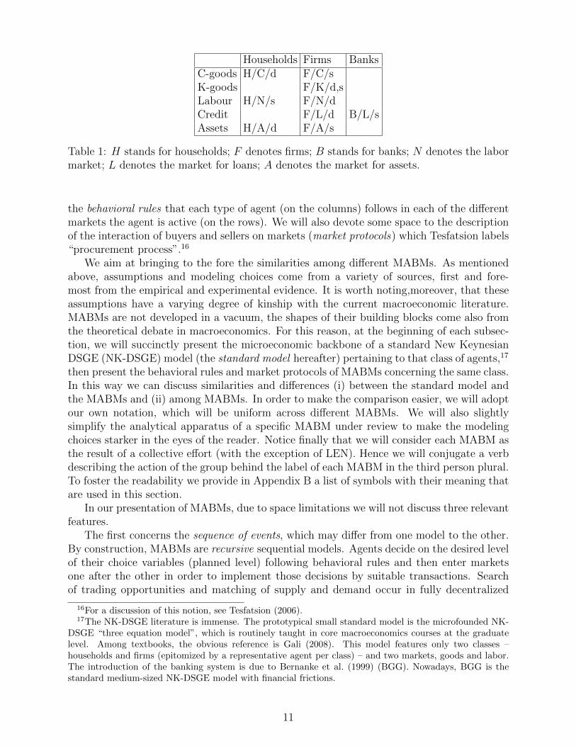
Households Firms BanksC-goods H/C/d F/C/sK-goods F/K/d,sLabour H/N/s F/N/dCredit F/L/d B/L/sAssets H/A/d F/A/s

Table 1: H stands for households; F denotes firms; B stands for banks; N denotes the labormarket; L denotes the market for loans; A denotes the market for assets.

the behavioral rules that each type of agent (on the columns) follows in each of the differentmarkets the agent is active (on the rows). We will also devote some space to the descriptionof the interaction of buyers and sellers on markets (market protocols) which Tesfatsion labels“procurement process”.16

We aim at bringing to the fore the similarities among different MABMs. As mentionedabove, assumptions and modeling choices come from a variety of sources, first and fore-most from the empirical and experimental evidence. It is worth noting,moreover, that theseassumptions have a varying degree of kinship with the current macroeconomic literature.MABMs are not developed in a vacuum, the shapes of their building blocks come also fromthe theoretical debate in macroeconomics. For this reason, at the beginning of each subsec-tion, we will succinctly present the microeconomic backbone of a standard New KeynesianDSGE (NK-DSGE) model (the standard model hereafter) pertaining to that class of agents,17

then present the behavioral rules and market protocols of MABMs concerning the same class.In this way we can discuss similarities and differences (i) between the standard model andthe MABMs and (ii) among MABMs. In order to make the comparison easier, we will adoptour own notation, which will be uniform across different MABMs. We will also slightlysimplify the analytical apparatus of a specific MABM under review to make the modelingchoices starker in the eyes of the reader. Notice finally that we will consider each MABM asthe result of a collective effort (with the exception of LEN). Hence we will conjugate a verbdescribing the action of the group behind the label of each MABM in the third person plural.To foster the readability we provide in Appendix B a list of symbols with their meaning thatare used in this section.

In our presentation of MABMs, due to space limitations we will not discuss three relevantfeatures.

The first concerns the sequence of events, which may differ from one model to the other.By construction, MABMs are recursive sequential models. Agents decide on the desired levelof their choice variables (planned level) following behavioral rules and then enter marketsone after the other in order to implement those decisions by suitable transactions. Searchof trading opportunities and matching of supply and demand occur in fully decentralized

16For a discussion of this notion, see Tesfatsion (2006).17The NK-DSGE literature is immense. The prototypical small standard model is the microfounded NK-

DSGE “three equation model”, which is routinely taught in core macroeconomics courses at the graduatelevel. Among textbooks, the obvious reference is Gali (2008). This model features only two classes –households and firms (epitomized by a representative agent per class) – and two markets, goods and labor.The introduction of the banking system is due to Bernanke et al. (1999) (BGG). Nowadays, BGG is thestandard medium-sized NK-DSGE model with financial frictions.

11

markets, i.e., in the absence of a top-down mechanism to enforce equilibrium. Therefore,transactions typically occur at prices which do not clear the market. This may cause adisruption of plans, which must be revised accordingly.

Consider, for instance, a C-firm. Once the quantity to be produced has been established,the firm determines desired employment. If desired employment is greater than the currentworkforce, the firm tries to hire new workers by posting vacancies. She may not be ableto fill the vacancies, however, because not enough workers will visit the firm or accept theposition.18 In this case, the firm has to downsize her production plans. Generally, dueto unexploited trading opportunities, three constraints may limit the implementation ofdecisions, e.g. firms may be unable to (i) find enough external funds to fill the financing gapand/or (ii) hire enough workers and/or (iii) acquire enough capital to implement the desiredlevel of production.

The second feature concerns time discretization. By construction, in MABMs time isdiscrete. MABMs can differ, however, as far as the minimal time unit is considered (a day,a week, a month, a quarter). Moreover, transactions can occur at different time scales. Forinstance, in LEN C-goods are traded every day but labor services are traded on a monthlybase. In the following, for simplicity we will not be specific on the time unit which will bereferred to with the generic term “a period”.

The third feature concerns the characterization of interaction. A few MABMs are net-worked, i.e. they have an explicit network structure: agents are linked by means of tradingrelationships which take the form of persistent partnerships. In LEN, for instance, eachhousehold trades with a finite set of firms.19 Most of the MABMs we will consider below,however, do not assume a fixed network of trading relationships. Partners in a trade todaymay not trade again tomorrow. In a sense, trading relationships de facto connect people ina network which is systematically reshuffled every period.20

2.3 Households

In the following, we will consider a population of H households. Variables pertaining to theh-th household will be denoted with the suffix h. Households may be active or inactive onthe labor market. If active, they supply labor (in most MABMs, labor supply is exogenous).In some MABMs, households searching the labour market have a reservation wage, whichmay be constant or decreasing with the length of the unemployment spell. If employed,the household earns a wage. In some MABMs, if unemployed the household receives anunemployment subsidy, which amounts to a fraction of the wage of employed households.

Households are also firm owners. Firm ownership may be limited to a fraction of inactivehouseholds or spread somehow also to active households. As a firm owner, the householdreceives dividends. Current income is the sum of the wage bill and dividends. Householdspurchase C-goods. Generally, households are surplus units, i.e., they do not get into debt.Unspent income is saved and generates financial wealth. In most MABMs, financial wealth

18In most MABMs the labour market is riddled with frictions: each unemployed worker visits only alimited number of firms and/or the posted vacancies are advertised only to a certain number of unemployedworkers. Hence, after a round of transactions on the market, there will still be unfilled vacancies as well asunemployed workers.

19This is also the case, for instance, of variants of the CATS framework, e.g. Delli Gatti et al. (2010).20To be precise, also in the case of networked MABMs, the network can be rewired. Typically, with a

certain probability and a certain periodicity, an agent switches from one partner to another.

12

consists of bank deposits only.In LEN, households are linked in a network of trading relationships to a finite set of

firms from which they buy C-goods and firms for which they work. Since there are no banks,households hold wealth in liquid form (money holding).

In AGH, each household (“person”) is denoted by the type (i, j) where i is the house-hold’s labor/product type and j are the types of goods the household wants to consume.By assumption the household consumes only two goods, different from the good she canproduce. The product type is isomorphic to the labour type.21 A household of type i canbe a worker if employed by a firm (“shop”) of the same type. If a worker, she earns a wage.Otherwise, the household can be a firm owner.

In the CATS framework, households can be either workers or “capitalists”. Workerssupply labor, earn a wage (if employed), consume and save. Capitalists are the ownersof firms. For simplicity there is one capitalist per firm. Capitalists earn dividends (if thefirm is profitable), consume and save (therefore they behave as rentiers). Both workersand capitalists accumulate their savings in the form of deposits at banks. If the firm goesbankrupt, the owner of the bankrupt firm employs his personal wealth to provide equity tothe entrant firm. In other words, the capitalist is de facto re-capitalizing the defaulting firmto make it survive.

In KS, EUBI, EUGE and LAGOM each household supplies labor and owns firms atthe same time. This alternative approach poses the problem of attributing ownership rights,dividends and recapitalization commitments to heterogeneous households. For instance, inEUBI, the household holds financial wealth in the form of deposits at banks and an indexof stocks which define property rights and the distribution of dividends.

In JAMEL, some of the households (chosen at random) are firm owners and remain firmowners for a certain time period (typically a run of a simulation).

2.3.1 The demand for consumption goods

In this section we will first recall the basic tenets of the standard model of household’sconsumption/saving decisions, which we will refer to as the Life Cycle/Permanent Income(LCPI) benchmark. We will then present the most general specification of the consumptionbehavioral rule which we can extract from the MABM literature. The specific behavioral rulesadopted by different MABMs can be conceived as special cases of this general specification.

The Life Cycle/Permanent Income benchmark The standard approach to house-holds’ behavior (incorporated in NK-DSGE models) is based on “two-stage budgeting”.In the first stage, the representative infinitely lived household maximizes expected lifetimeutility subject to the intertemporal budget constraint, determining the optimal size of con-sumption expenditure Ch,t, which we will sometimes refer to hereafter as the consumptionbudget.

In the second stage the household determines the composition of Ch,t, i.e., the fractionCi,h,t/Ch,t for each variety i = 1, 2, .., Fc where Fc is the cardinality of the set of C-goods(and of C-firms).22

21In other words, technology is one-to-one. Each household is endowed with a unit of specific labor – say,labor of the i-th type – so that she can produce one unit of the i-th product.

22By construction, in a Dixit-Stiglitz setting Ch,t is a CES aggregator of individual quantities.

13

As far as the first stage is concerned, optimal consumption turns out to be a functionof expected future consumption EtCh,t+1 and the real interest rate r (consumption Eulerequation).

Notice now that consumption expenditure is equal by definition to permanent income:Ch,t = Y p

h,t. Hence, after some algebra, we get

Ch,t = r(W hh,t +W f

h,t) (1)

where r = R − 1 is the (net, real) interest rate, W hh,t is human capital and W f

h,t is financialwealth. Equation (1) can be interpreted as a benchmark Life Cycle/Permanent Income(LCPI) consumption function. In this framework, by construction, the consumption budgetis equal to the annuity value of total (financial and human) wealth.

Human capital, in turn, is defined as the discounted sum of current income and expectedfuture incomes accruing to the household:

W hh,t =

1

R

∞∑s=0

(1

R

)sEtYh,t+s =

1

RYh,t +

1

R

∞∑s=1

(1

R

)sEtYh,t+s (2)

Substituting (2) into (1), the LCPI consumption function becomes:

Ch,t =r

RYh,t +

r

R

∞∑s=1

(1

R

)sEtYh,t+s + rW f

h,t (3)

In words: consumption is a linear function of current and expected future incomes and offinancial wealth.

By definition, in the LCPI benchmark, W fh,t+1 = RW f

h,t + Yh,t − Ch,t. Therefore saving

– i.e. the change in financial wealth Sh,t = W fh,t+1 −W

fh,t – turns out to be equal to Sh,t =

rW fh,t +Yh,t−Ch,t. Since consumption is equal to permanent income, saving can be specified

as follows:Sh,t = rW f

h,t + (Yh,t − Y ph,t) (4)

where the expression in parentheses is transitory income. All the income in excess of per-manent income will be saved and added to financial wealth. If, on the other hand, currentincome falls short of permanent income, the household will stabilize consumption by decu-mulating financial wealth.

As far as the second stage is concerned, it is easy to show that in a Dixit-Stiglitz frame-work the (optimal) fraction of each good in the bundle is

Ci,h,tCh,t

=

(Pi,tPt

)−ε(5)

where Pi,t is the price of the i-th variety, Pt is the general price level 23 and ε is the absolutevalue of the price elasticity of demand. In words: the fraction of the consumption budgetallocated to each variety is a decreasing function of the relative price

Pi,tPt

.Generally, households are assumed to be identical. If household members are heteroge-

neous (for instance because of the employment status, or the level and the source of income),

23By construction, the general price level is a CES aggregator of individual prices.

14

in standard models complete markets are assumed so that idiosyncratic risk can always beinsured. Within the household, “full consumption insurance” follows from the assumptionthat household members pool together their incomes (wages, unemployment subsidies, divi-dends) and consume the same amount in the same proportions. Thanks to this assumption,heterogeneity, albeit present, is irrelevant because the household may still be dealt with as aunique (representative) agent. If idiosyncratic income risk is uninsurable, then heterogeneitycannot be assumed away.24

The Agent Based approach to consumption/saving decisions A two stage proce-dure is also generally adopted in MABMs. In the first stage household h determines theconsumption budget Ch,t, i.e., the amount of resources (income, wealth) to be allocated toconsumption expenditure. In the second stage the household determines the compositionof the bundle of consumption goods, i.e., the quantities Ci,h,t, i = 1, 2, ...Fc of the goodswhich enter the consumption bundle. Notice however that, in general, agents do not followexplicit optimization procedures. Markets are generally incomplete and within-householdconsumption insurance is ruled out.

The choice of the consumption budgetAs far as the first stage is concerned, the most general behavioral rule adopted to set theconsumption budget in the MABM literature can be specified as follows:

Ch,t = chWhh,t + cfW

fh,t (6)

where W fh,t is the household’s financial wealth (deposited at the bank and/or invested in

financial assets), W hh,t is human capital, ch and cf are propensities to consume, both positive

and smaller than one. In words, consumption is a linear function of human and financialwealth.

By definition W fh,t = RW f

h,t−1 + Yh,t − Ch,t and Sh,t = W fh,t −W f

h,t−1. Consumption isdefined as in (6). Hence, in a generic MABM savings turn out to be:

Sh,t = Yh,t + (r − cf )W fh,t−1 − chW

hh,t (7)

If positive, savings increase financial wealth. In some MABMs saving can be involuntary:it may happen that the household cannot find enough consumption goods at the limitednumber of firms she visits. Saving will turn negative – i.e. the household will decumulatefinancial wealth – if the consumer does not receive income – for instance because a workerbecomes unemployed and/or financial income (interest payments on financial wealth) is toolow. In most MABMs household do not get into debt so that consumption smoothing islimited or absent (in the jargon of NK-DSGE models, asset market participation is limited).

Specifications of the general rule (6) differ from one MABM to the other.AGH set ch = cf = c. Moreover, they define human capital as the capitalized value of

permanent income W hh,t = khY p

h,t where kh is a capitalization factor25. Permanent income

24Incomplete markets is the basic assumption of the literature on Standard Incomplete Market (SIM)models with heterogeneous agents, both of the new Classical and New Keynesian type. The New Keynesianvariants are known as Heterogeneous Agents New Keynesian (HANK) models. For an exhaustive survey, seethe chapter by Ragot in this Handbook.

25in AGH kh is endogenous as it is a function of projections of inflation and the interest rate elaboratedby the central bank and made available to the general public.

15

Y ph,t is computed by means of an adaptive algorithm: Y p

h,t − Yph,t−1 = (1− ξ)

(Yh,t−1 − Y p

h,t−1

)where ξ ∈ (0, 1) is a memory parameter. By iterating, it is easy to see that permanentincome (and therefore human capital) turns out to be a weighted sum of past incomes only:Y ph,t = (1− ξ)

∑−∞s=0 ξ

sYh,t−s−1. Hence the AGH behavioral rule for consumption expenditureis

Ch,t = ckh(1− ξ)−∞∑s=0

ξsYh,t−s−1 + cW fh,t (8)

In words, consumption is a linear function of past incomes and financial wealth.In the CATS/ADG framework, human capital is defined by the following adaptive

algorithm: W hh,t = ξW h

h,t−1 + (1 − ξ)Yh,t. By iterating, one gets W hh,t = (1 − ξ)Yh,t + (1 −

ξ)∑−∞

s=1 ξsYh,t−s i.e., human capital is a weighted average of current and past incomes.26

Substituting this definition into (6) the behavioral rule specializes to

Ch,t = ch(1− ξ)Yh,t + ch(1− ξ)−∞∑s=1

ξsYh,t−s + cfWfh,t (9)

While human capital in the neoclassical approach is a linear combination of current andexpected future incomes, and therefore is formed in a forward looking way, the proxy forhuman capital in AGH and CATS/ADG is a linear combination of current and past incomes,i.e. it is determined by a backward looking algorithm.27

Setting ξ = 0 – i.e., assuming that there is no memory – human capital boils down tocurrent income, so that (9) specializes to:

Ch,t = cyYh,t + cfWfh,t (10)

where cy is the propensity to consume out of income.28

Setting cf = 0, from (10) we get a specification of the consumption function sometimesadopted in MABMs of a strictly Keynesian flavor

Ch,t = cyYh,t (11)

In many models of the KS family, the behavioural rule is (11) with ch = 1:

Ch,t = Yh,t (12)

This specification describes the behaviour of “Hand to mouth” consumers.29

26In ADG income accruing to the household is Yh,t = w if the consumer is a worker with an active laborcontract, Yf,t = τπf,t−1 if the consumer is a capitalist receiving dividends; τ is the dividend-payout ratioand πf,t−1 are profits of the firm realized in the previous period and accruing as income to the capitalist inthe current period.

27This difference reflects the fact that forward looking expectation formation is marred with insurmount-able difficulties in a complex heterogeneous agents context.In this context, the obvious candidate for expec-tation formation is an adaptive algorithm. Notice, however, that the empirical work on consumption hasextensively used adaptive algorithms.

28cy in (10) coincides with ch in (9) because, in the absence of memory, human capital coincides withcurrent income.

29This is the specification used in NK models with “Rule of thumb” consumers, i.e. consumers who cannotsmooth consumption over the life cycle due to “limited asset market participation” or “liquidity constraints”.

16

LAGOM adopts a rule such as (10) with cy = 0. Moreover, since financial wealth

coincides with money holding (W fh,t =

Mh,t

Pt), the consumption budget turns out to be an

increasing linear function of real money balances:30

Ch,t = cfMh,t

Pt(13)

In CATS/DD, consumption is a special case of (10) obtained by setting cy = cf = c.Therefore:

Ch,t = c(Yh,t +W fh,t) (14)

The expression in parentheses is one of the possible specifications of “cash on hand”. Cash-on-hand can be defined in the most general way as liquid assets which can be used to carryon transactions. In small MABMs which do not feature banks such as LEN, cash-on-handcoincides with currency. In a setting with banks such as CATS/DD, cash on hand coincideswith new deposits, which in turn amount to the sum of income and old deposits. This isin line with Deaton (1991)), who defines cash on hand as the sum of income and financialassets.

In EUBI and EUGE saving behavior aims at achieving a target for wealth: Sh,t =

ν(ωfYh,t − W fh,t) where ωf is the target wealth-to-income ratio and ν is the velocity of

adjustment of wealth to targeted wealth. Since, by definition Sh,t = Yh,t − Ch,t, simplealgebra shows that under this assumption the consumption budget can be written as:

Ch,t = (1− νωf )Yh,t + νW fh,t (15)

which is a special case of (10) with cy = 1− νωf and cf = ν.Carroll has shown that in an uncertain world consumption is a concave function of cash-

on-hand which he defines as the sum of human capital and beginning of period wealth.31

In Carroll’s framework, for low values of wealth, the propensity to consume (out of wealth)is high due to the precautionary motive: a reduction of wealth would in fact lead to asizable reduction of consumption to rebuild wealth (buffer stock rule). In some MABMs theconsumption function is adjusted to mimic Carroll’s precautionary motive, i.e., to reproducethe non linearity of the relationship between consumption and wealth. This theoreticalsetting has been corroborated by a number of empirical studies (see Carroll and Summers(1991), Carroll (1997)), such that using this approach in MABMs is consistent with theagenda to rely on behavioral rules which have strong empirical foundations.

For instance in EUBI, the specification of the consumption function discussed abovegives rise to a piecewise linear heuristic based on the buffer-stock rule. Also EUGE adopt aspecification of the consumption budget which adopts Carroll’s rule.

In the CATS/MBU framework consumption is specified as in (11) but cy is a non-linearfunction of wealth. This allows to capture the interaction between income and wealth in thedetermination of consumption.

30In LAGOM firms enter the market for C-goods to purchase raw materials and wholesale goods (cir-culating capital). The demand for C-goods of the i-th firm is Kc

i,t = (1/kc)Y T − Kci,t−1 where Y T is the

production target of the firm, kc is the marginal productivity of circulating capital and Kci,t−1 is the stock

of circulating capital inherited from the past.31See Carroll (1992, 1997, 2009).

17

LEN explicitly models the consumption budget as an increasing concave function ofmoney holdings:

Ch,t =

(Mh,t

Pt

)c(16)

where c ∈ (0, 1).32

JAMEL presents a variant of Carroll’s framework. The household computes “averageincome” (which can be considered a proxy of permanent income) as the mean of incomesreceived over a certain time span occurred in the past: Y a

h,t = 1n

∑tτ=t−n Yh,τ .

33 Moreover,JAMEL define desired or targeted cash on hand as a fraction of average income: mT

h,t = sY ah,t,

where mTh,t = MT

h,t/Pt are real money balances and s ∈ (0, 1) is the desired propensity tosave (out of average income). The consumption budget is defined as follows:

Ch,t =

cY a

h,t if mh,t < mTh,t

Y ah,t + cm

(mh,t −mT

h,t

)if mh,t > mT

h,t

(17)

where c = 1 − s and cm ∈ (0, 1) is the propensity to consume. In words: if liquid assetsare (relatively) “low”, the household spends a fraction c of average income. If liquidity is“high”, the household consumes the entire average income and a fraction cm of excess moneybalances, defined as the difference between the current and targeted money holding.

With the help of some algebra, the behavioral rule above can be written as follows:

Ch,t =

cY a

h,t if Y ah,t > Y a

h,t

c′Y ah,t + cmMh,t if Y a

h,t < Y ah,t

(18)

where Y ah,t = 1

smh,t is the cut-off value of average income and c′ = 1−cm(1−c) = (1−cm)(1−

c)+ c. Notice that c′ > c. The cut-off value of average income is a multiple of current moneyholdings. The specification above highlights the basic tenets of Carroll’s buffer stock theoryin a very simple piece-wise linear setting. When average income is below the threshold – i.e.when the threshold is relatively high because the household is wealthy/liquid – the marginalpropensity to consume is c′ i.e., it is relatively high. When average income surpasses thethreshold the marginal propensity drops to c.

JAMEL also incorporates consumer sentiment and opinion dynamics in the consumptionfunction. The propensity to save s can take on two values. When “optimistic”, the householdis characterized by sL while if “pessimistic” she sets s to sH , with sH > sL. Pessimism leadsto a reduction of the propensity to consume: households save more for rainy days.

Each household switches from a low to a high propensity to save (and vice versa) de-pending on her employment status. The household turns pessimistic if unemployed. In eachperiod, the household observes the consumer sentiment (proxied by the employment status)of a finite subset of other households (a neighborhood for short). With probability πm sheadopts the majority opinion – i.e. the prevailing consumer sentiment – of the neighborhood;with probability 1 − πm the household relies on her own situation: if she is unemployed

32Of course, consumption cannot be greater than money holding. Hence (Mh,t/Pt) > 133In JAMEL the minimal time unit is a month. Yh,t therefore is current income in month t. Average

income in month t is the mean of monthly incomes in the last 12 months up to t, i.e. Y ah,t = 112

∑tτ=t−12 Yh,τ .

Since permanent income is the weighted average of all the past incomes over an infinite time span withexponentially decaying weights (see above), average income is defined on a shorter time span and with equalinstead of decaying weights.

18

(employed), she will be pessimistic (optimistic) and will choose sH (sL). The probability ofadopting the sentiment of the majority can be interpreted as the strength of the households’“animal spirits”.

The choice of the goods to buy As to the second stage, the choice of the goods to buyis generally influenced by the relative price. EUBI and EUGE introduce a multinomial logitmodel, CATS posit a search mechanism.

In LEN each household is linked to a fixed number of firms from which she can buy.The network can change over time. Each period, with a certain probability, the householdchooses at random a firm in the neighborhood of current trading partners and a firm outsideit, compares the prices and switches to the new firm if the price of the price set by thecurrent partner exceeds the price of the new firm by at least a certain margin. In the end,therefore, the household searches for better trading opportunities based on relative price.34

AGH posit that the household can buy only from two firms (“stores”, i.e., shops wherethe household purchases her consumption goods). Hence she has to choose the quantity tobe demanded from each firm. AGH derives behavioral rules by solving a simple optimizationproblem. The household maximizes Uh,t = U(C1,h,t, C2,h,t) subject to p1,tC1,h,t + p2,tC2,h,t =

Ch,t where pi,t =Pi,tPt

, i = 1, 2. Hence the quantity demanded for each variety turns out tobe:

Ci,h,t = fi(p1,t, p2,t, Ch,t) i = 1, 2 (19)

which can be easily compared with (22). The household explores the goods market lookingfor stores supplying the goods she wants to consume. The household buys from store j onlyif the posted price Pj,t is smaller than a reservation price equal to the price paid by thehousehold in the past Ph,j,t−1 (appropriately indexed): Ph,i,t−1(1 + πT ) > Pj,t where πT isexpected inflation, anchored to the inflation target of the central bank.35

In the CATS framework, households collect information and pick goods by visitingfirms chosen at random. The h-th household visits Zc randomly selected firms, ranks themaccording to the price they charge and purchases C-goods starting from the firm chargingthe lowest price. If she does not spend the entire consumption budget at the first firm,she will move up to the second firm in the ranking and so on. If she has not spent all theconsumption budget after visiting Zc firms, she will save involuntarily. This implies that thedemand for the good produced by the i-th C-firm is implicitly decreasing with the relativeprice pi,t. Notice however that the implicit demand curve that the i-th firm is facing isshifting over time. A given firm may be visited by different sets of consumers on subsequentdays. The search and matching mechanism leads to the coexistence of queues of unsatisfiedconsumers (involuntary savers) at some firms and involuntary inventories of unsold goods atsome other firms.

LAGOM adopts a similar market protocol as CATS for the market for C-goods. Inthe LAGOM model also firms enter the market for C-goods as they use circulating capitaltogether with fixed capital for production.

EUBI and EUGE assume that the consumer receives information about the range ofproducts, their prices and their availability at (local) malls. The choice of the good to buy

34The household leaves the current partner and switches to a different one also when the household isdemand constrained, i.e., when current trading partners are unable to satisfy demand.

35Of course, this assumption is implicitly based on the credibility of the central bank’s announced inflationtarget.

19

is random and the probability of buying a certain product is determined by a multinomiallogit model:

P [consumer h selects good i] =exp(−γlogPi,t)∑j exp(−γlogPj,t)

(20)

where the sum in the denominator includes all products for which the consumer has receivedinformation.36 As has been discussed in Dawid et al. (2018c) this formulation can also beinterpreted as a representation of a situation in which the product offered by the differentC-firms are horizontally differentiated along dimensions not explicitly captured in the model.The parameter γ governs the intensity of (price) competition between the C-firms and typi-cally has strong influence on the emerging economic dynamics on the aggregate level. Dawidet al. (2018c) also point out that the use of logit-choice models for the representation ofconsumer choice has strong empirical foundations, e.g. in the Marketing literature.37

2.3.2 Labour supply

On the labour market, households are suppliers of labor. The h-th worker supplies inelasti-cally one unit of labor.

LEN assumes that each household has a reservation wage, denoted with wh. She suppliesher labor only to a finite subset of the population of firms, a neighborhood of potentialemployers. However, the network can be re-wired. If the household is employed, say, at firmi, and her current wage is higher than the reservation wage (wi > wh), she will search fora better position infrequently, i.e. with probability less than one. When searching, she willvisit only one new firm chosen at random. If at this new firm, say j, she finds wj > wi, shewill quit the current job and move to the j-th firm. If, for any reasons, her current wage fallsbelow the reservation wage (wi < wh),

38, she will intensify the quest for a better position byexploring a new firm every period (i.e., with certainty). If the household is unemployed, shewill search for a job every period by visiting a fixed number Ze of firms chosen at random.If the household switches to a new employer, the former employer drops out of the set ofemployers of the households and is replaced by the new one.

Also in LAGOM each household has a reservation wage. If the household is employed,say, at firm i, and her current wage is lower than the reservation wage (wi < wh), she willquit her job and search for a better position at a finite set of firms chosen at random.

In AGH, as we saw above, a household type is defined by the production good it canproduce with its labor type. If employed, the household is working in the same firm whichproduces her production good. If unemployed, the household engages in job search with agiven probability πs. She explore the labor market looking for a firm (with the same producttype) posting a vacancy. The household accepts the job offer if her previous wage wh,i,t−1

(appropriately indexed) is smaller than the posted wage wi,t, i.e., if wh,i,t−1(1 + πT ) < wi,t.In CATS/MBU and CATS/ADG, the h-th household, if unemployed, looks for a

job by visiting Ze firms chosen at random and applying to those with open vacancies. InCATS/MBU the posted wage is firm-specific and cannot drop below a lower bound repre-sented by a minimum wage, which is changing over time due to indexation. The unemployed

36In Dawid et al. (2018b) this setting is extended by assuming that consumers have a ’home-bias’ inconsumption, such that the attractiveness of a product depends in addition to the price also on the factwhether it has been produced by a firm located in the same region as the consumer.

37An axiomatic behavioral foundation for multinomial logit models can be found in Breitmoser (2016).38This case may be due to the decision of the firm to cut the posted wage

20

worker will accept a job from the firm with open vacancies which pays the higher wage.For simplicity in CATS/ADG the posted wage is given and uniform across firms so thatthe unemployed worker accept the job at the first chance of finding an open vacancy. If shedoesn’t find an open vacancy, the household remains unemployed and funds her consumptionby dis-saving, i.e. consuming out of accumulated wealth. For simplicity CATS assume thatthere are neither hiring nor firing costs. If a firm wants to scale down activity in a certainperiod, it can fire workers at no costs. Fired workers become unemployed and start searchingfor a job in the same period.

In EUBI the household is characterized by a specific skill and has a reservation wage. Ifunemployed, she explores the labor market with a given probability. Firms post vacanciesand wages. The unemployed household ranks the wage offers and applies only to firms thatmake a wage offer (for the worker’s skill group) which is higher than her reservation wage. Ifthe unemployed job searcher receives several acceptable job offers she accepts the offer withthe highest wage. The reservation wage of the worker is adjusted downwards during periodsof unemployment.

In JAMEL, the household’s reservation wage is stochastically reduced if the unemploy-ment spell is greater than an exogenous upper bound. In symbols:

wh,t =

wh,t−1(1− ηh) if duh,t > du

wh,t−1 if duh,t < du(21)

where ηh ≥ 0 is a random draw from a uniform distribution, duh,t is the duration of the

unemployment spell and du is the threshold value of this spell.

2.3.3 The demand for financial assets

In a small MABM such as LEN, households can hold wealth only in the most liquid form(cash). Most medium-sized MABMs assume that there is at least one other financial assetsuch as deposits at banks. For CATS, KS, JAMEL, LAGOM households’ wealth consistsonly of deposits. In AGH, households can hold cash, deposits and Government bonds. InEUBI and EUGE the household can hold wealth as liquidity (deposits at banks), as aportfolio of shares issued by firms and banks and in EUGE also as government bonds.Households therefore, receive dividends according to the composition of their portfolio ofshares. For simplicity, in EUBI the allocation of households’ savings to bank deposits andshares is random. Modeling the portfolio choice for each household, however, may be quitecomplex. For instance, the preference structure of “investors” in EUGE – i.e., householdswho trade in financial markets – takes into account insights from behavioral finance, namelymyopic loss aversion. Transactions on financial markets occur at higher frequency than onreal markets (daily as against monthly). Prices are determined in equilibrium through aclearinghouse mechanism. In CATS households can be of two types, workers and capitalists.Assuming that there is one capitalist per firm, each firm distributes part of its profits to thefirm owner as dividends. KS adopt the extreme assumption that all the profits are retainedwithin the firm and used to accumulate net worth. In this case, by assumption there will beno dividends. In JAMEL some households (chosen at random) are firm owners and thereforereceive dividends which will be distributed only if the firm’s net worth is higher than athreshold (defined by a target level for leverage). Opinion dynamics play a role in dividenddistribution. Firms switch from “optimistic”, (characterized by high target leverage and

21

high dividends) to “pessimistic” (low target leverage and low dividends). Also in LAGOMhouseholds are firm owners and receive both wages and dividends.

2.4 Firms

In this section we will consider a population of F firms, which produce either consumptiongoods (C-firms) or capital goods (K-firms). Variables pertaining to the i-th C-firm will bedenoted with the index i = 1, 2, ...Fc. Variables pertaining to the k-th K-firm will be denotedwith the index k = 1, 2, ...Fk. In most MABMs C-firms demand labor and K-goods in orderto produce and sell C-goods to households; K-firms demand labor in order to produce andsell K-goods to C-firms.39.

Firms have market power, hence they set the quantity and the price of the goods theyproduce and sell. Generally, market power is rooted in transaction costs. Due to uncertaintyand the costs of exploring market conditions, in fact, buyers do not have enough informationon the prices and quantities set by all the sellers so that they purchase goods from a limitedset of suppliers. Each supplier, therefore, operates in condition of monopolistic competitionor oligopoly on the market for her own good.

The planned (or desired) scale of activity is the main determinant of the demand forinputs, namely the demand for capital and the demand for labor.

On the market for K-goods, demand comes from C-firms and supply comes from K-firms.The i-th C-firm’s demand for K-goods – i.e. investment – is driven mainly by productionrequirements. If production planned in t for t+1 can be carried out with the capital stockinherited from the past (after depreciation), the firm simply adjusts capacity utilization.If capital inherited from the past is insufficient to undertake planned production, the i-thfirm should expand capacity by purchasing new K-goods (sometimes referred to as “machinetools”). In some MABMS, this is feasible. In other MABMs, investment in t is driven bylong run production requirements and cannot be used to face short run peaks of demand.Hence the firm will be constrained to produce at full capacity but less than desired.

On the market for labour, demand comes from all the firms and supply comes fromhouseholds. Firms whose workforce is insufficient to undertake planned production will postvacancies and a wage offer (which may be firm-specific or uniform across firms, constant ortime-varying because of indexation and/or because of labour market conditions.)

Firms may have a financing gap, i.e., a positive difference between operating costs andinternally generated funds. They generally ask for a loan to fill this gap. The quantity andprice of credit are set by banks.

Firms may be unable to achieve the desired scale of activity for lack of funds (if theyare rationed on the credit market), of capital (if investment is disconnected from short runproduction need and/or if they don’t find enough machine tools to buy) or of labor (if theydon’t find enough workers to hire).

2.4.1 The supply of consumption goods

The Dixit-Stiglitz benchmark As far as the corporate sector is concerned, NK DSGEmodels are based on monopolistic competition: each firm behaves as a monopolist on her ownmarket. The firm’s market power is due to product heterogeneity. Products may be different

39In some MABMs, firms use also raw materials, energy and wholesale/intermediate goods as inputs. Wewill be more specific below.

22

in the eyes of consumers for a number of reasons: spatial dispersion, product differentiationor transaction costs which may generate captive markets.

In the Dixit-Stiglitz benchmark, the demand of the h-th household for the i-th good isrepresented by equation (5). Summing across H households and rearranging one gets thedemand function for the i-th good:

Ci,t =

(Pi,tPt

)−εCtFc

(22)

where Ct =∑H

h=1Ch,t is total consumption (economywide).40

With a linear technology and only the labour input, the marginal cost will be wt/α wherewt is the wage and α is the marginal productivity of labor. Optimal pricing yields

P ∗i,t = (1 + µ)wtα

(23)

where µ = (ε− 1)−1 is the mark-up.Substituting (23) into (22) one gets the optimal scale of production:

Y ∗i,t = C∗i,t =

(1 + µ

α

wtPt

)−εCtFc

(24)

Since the manager of the firm knows the production function and input costs, and there-fore can compute the marginal cost, if she knows also the demand curve she will choose anoptimal mark up (i.e., ratio of the individual price to marginal cost) and an optimal scaleof activity. In other words, in the absence of uncertainty on market demand, the firm willchoose a point on the demand curve in such a way as to maximize profits. In this case supplywill always be equal to demand: the firm will neither accumulate involuntary inventories ofunsold goods nor face queues of unsatisfied consumers: output will always be sold and nopotential customer will leave the firm’s premises empty handed.

Moreover, in the absence of frictions on the labour market, the firm will always be ableto carry out planned production. In the end therefore planned output will be equal to actualoutput and actual output will be equal to sales.

From (23) and (24) we can predict the following: the firm will react to (i) an increaseof elasticity of demand by reducing the mark up and therefore the individual price andincreasing production; (ii) an increase of the real wage by increasing the price and reducingproduction; (iii) an increase in productivity by reducing the price and increasing production,(iv) an increase in total consumption by increasing production.

Since firms have the same technology, incur the same labour cost and face the samedemand function, a symmetric equilibrium in which all firms charge the same price, is con-sidered: Pi,t = Pt, so that the real wage will be equal to (wt/Pt)

∗ = α/(1 + µ). At thatwage, employment is determined by labor supply, the labour market clears and there is fullemployment.41Total output is equal to the full employment level of GDP.42 In the absence

40For the sake of comparison with MABMs, equation (22) concerns the case of a “large” but finite numberof firms. Equation (5) is derived assuming a continuum of firms of unit mass.

41In the standard model labor supply derives from expected lifetime utility maximization when leisure is anargument of the period utility function. It turns out that labor supply is increasing with the real wage. Thereal wage in the symmetric equilibrium with monopolistic competition is smaller than in perfect competition,because in the latter case the mark up is zero. Hence full employment with monopolistic competition willbe smaller than in the case of perfect competition.

42This is the characterization of total output in the equilibrium with flexible prices of the standard NKDSGE model.

23

of investment, output is equal to consumption. Each firm therefore will produce the samequantity, i.e., a fraction 1/Fc of total consumption, which is equal to total full employmentoutput. In the presence of nominal rigidities (e.g. Calvo pricing), this level of output isunattainable, at least in the short run.

Price/quantity decisions when demand is unknown In order to understand theprice/quantity strategies of firms in MABMs and compare them with firms’ decisions in thestandard model, in this “intermezzo” we will keep the basic structure of the Dixit-Stiglitzframework but will relax the assumption of perfect information as far as market demand isconcerned. We will assume instead that, at the moment decisions on price and quantity mustbe made, the firm does not know the position of the demand curve on the price/quantityspace.

Uncertainty on market demand may be due to the fact that transactions do not occurat the same time on all markets. There is a sequence of events which take place at differenttimes on different markets. For instance we can envisage the following 4 steps. (1) At thebeginning of period t (before the market for C-goods opens), the firm decides the priceand the quantity. On the basis of the production plan, it decides whether to hire or fireworkers. Suppose the workforce must be expanded to fulfill the production plan. (2) Thefirm enters the labor market by posting vacancies at a certain wage. These vacancies mayor may not be filled depending on the number of matches between demand (job offers) andsupply (unemployed workers) of labor. Suppose all the vacancies are filled. (3) The firm cantherefore implement the desired production plan. (4) The quantity produced is then sold onthe market of C-goods. Production must be decided in step (1) but actual demand will berevealed to the firm only in step (4).

The information set of the firm at the moment the scale of activity must be decided maycontain precise information on the pricing behavior of competitors and the total number offirms but information may be incomplete and imperfect on the price elasticity of demandand/or total households’ consumption. In order to maximize expected profits, the firm mustestimate the elasticity of demand and total consumption planned by households. The marketdemand that the i-th firm expects is:

Cei,t =

(Pi,tPt

)−εit Cit

Fc(25)

where εit and Cit are price elasticity and total consumption expected or estimated by firm i.

In order to maximize profits in this informational scenario, the firm could set the price as amark up over marginal cost, the mark up being a function of the estimated price elasticity:

Pi,t =1 + µitα

wt (26)

where µit = (εit − 1)−1. Plugging (26) into (25) one gets:

Cei,t =

(1 + µitα

wtPt

)−εit Cit

Fc(27)

The firm uses expected demand to plan production: Y ∗i,t = Cei,t. For the sake of discussion,

24

let’s assume that actual production is equal to desired production: Yi,t = Y ∗i,t. Hence:43

Yi,t = Y ∗i,t = Cei,t =

(1 + µitα

wtPt

)−εit Cit

Fc(28)

At the beginning of time (step (1) in the sequence above) t the status quo for the i-thfirm is the point (Pi,t, Yi,t) on the price/quantity space. The coordinates are determined by(26) and (28). Once production has been carried out, transactions can take place. Oncetransactions are completed, the i-th firm can observe the amount of goods actually soldQi,t = min(Yi,t, Ci,t) where Ci,t is actual demand.

Since sales occur only after the firm has carried out production, actual demand can differfrom current production. If Qi,t = Ci,t < Yi,t, there will be involuntary inventories whosesize is: ∆i,t = Yi,t − Ci,t > 0. This is a signal of excess supply, i.e. of a positive forecastingerror (demand has been overestimated).

If Qi,t = Yi,t < Ci,t, all the output will be sold and therefore there will not be involuntaryinventories: ∆i,t = 0. The difference Yi,t − Ci,t > 0 measures the demand of unsatisfied con-sumers, who may turn to other producers (goods are substitutable, albeit only imperfectly)or save involuntarily. This is a signal of excess demand. The firm has made a negativeforecasting error (demand has been underestimated).

It can also happen, of course, that demand equals production: Yi,t = Ci,t. There will beno forecasting error (no inventories and no queues) in this case.

Inventories are defined as:

∆i,t = min(Yi,t − Ci,t, 0) (29)

In the case of excess demand or excess supply the firm is under-performing,44 and has anincentive to choose a different price/quantity in the future, say (Pi,t+1, Yi,t+1).

One possible strategy consists in setting the direction of the change in price and quantityin line with the sign of the forecasting error. For instance, if ∆i,t > 0 the firm has an incentiveto scale down production and cut the price. The size of the change may be linked to themagnitude of the error.

Notice that by making mistakes the firm collects new information on market conditions.As an alternative strategy, the firm can therefore make new estimates of demand and set theprice and the quantity accordingly (see equations (26) and (28)).

In the end, uncertainty and imperfect knowledge induce the firm to adapt period byperiod to evolving market conditions. This adaptation takes the form of price and quantityupdating rules. There is no guarantee that this adaptation will lead to the type of equilibriumdiscussed above.

The Agent Based approach to price/quantity decisions The MABMs we are survey-ing generally conceive firms as production/trading units immersed in a market environmentwhich is utterly uncertain. Uncertainty is due to the sequential nature of the market economy(which is easily replicated in an agent based framework) and to the ever changing conditionsof demand and supply.

43Notice that, in principle, desired production may not always be carried out because there may beconstraints on the attainment of planned production. For instance, in step (2) of the sequence above, not allthe vacancies may be filled. Therefore, in step (3) the firm cannot implement the desired scale of activity.

44In other words, the level of profits is smaller than in the optimal position.

25

Different MABMs deal with price/quantity strategies in different ways. For most of themodels we can detect a general pattern, however, in the description of the behavioral rulesthe firm adopts.45 The firm starts with an initial pair of price and quantity, (Pi,t, Yi,t), whichwe define the status quo. At the end of period t, once transactions have been carried out, thefirm observes actual sales Qi,t = min(Yi,t, Ci,t) and learns also the average price Pt, which isa proxy of the price charged on average by the firms’ competitors.

If Qi,t = Ci,t < Yi,t, there will be an inventory equal to ∆i,t = Yi,t −Ci,t > 0. Notice thatthe firm may want to hold a buffer stock of finished goods (desired or voluntary or targetinventories). Desired inventories may be an interval: ∆i,t ∈ ∆m

i,t,∆Mi,t – where the extremes

are the minimum and maximum levels of desired inventories – or collapse to a single point:∆∗i,t. In the first case there will be a shortage of inventories if ∆i,t < ∆m

i,t and excess (orinvoluntary) inventories ∆u

i,t = ∆i,t −∆Mi,t if ∆i,t > ∆M

i,t . In the second case there will be ashortage of inventories (resp. involuntary inventories) if ∆i,t < ∆∗i,t (resp. ∆i,t > ∆∗i,t). It isreasonable to assume that planned production for period t will take into account expecteddemand in the same period and desired inventories.

Of course desired inventories may be zero: ∆∗i,t = 0. In this case, planned production isequal to expected demand, Yi,t = Ce

i,t, the difference ei,t = Ci,t − Yi,t = Ci,t − Cei,t therefore

is the forecasting error. A positive inventory will always be involuntary and coincide withthe absolute value of the (negative) forecasting error: ei,t < 0 and ∆i,t = |ei,t| > 0. IfQi,t = Yi,t < Ci,t, the forecasting error is positive (ei,t > 0), there are no inventories (∆i,t = 0)but a fringe of unsatisfied consumers.

Desired inventories are generally determined by applying a desired or target inventory-to-sales ratio δ∗ to current production ∆∗i,t = δ∗Yi,t. This ratio represents the number of periodsof production at the current rate necessary to build desired inventories. Hence the minimumand maximum levels of voluntary inventories are determined as follows: ∆m

i,t = δmYi,t and∆Mi,t = δMYi,t, 0 < δm < δM . The parameters δm and δM are the minimum and the maximum

inventory-to-sales ratios. If there are no desired inventories, then δ∗ = 0.The firm receives two types of signals of market conditions: (i) an excess or shortage of

inventories (with respect to the target, which may be an interval, a positive value or zero);(ii) the relative price, i.e. the ratio or difference between the individual price and averageprice. From signals of type (i) the firm infers that it has underestimated or overestimatedthe strength of demand: a shortage of inventories reveals stronger than expected demand;an involuntary inventory signals weaker than expected demand. From signals of type (ii) thefirm infers its position relative to competitors: if the firm’s price is lower than the averageprice, the firm is undercutting competitors (and its market share is bigger than the averagemarket share); if the opposite holds true, the good produced by the firm is overpriced withrespect to competitors (and its market share is smaller than the average market share).46.The sign and size of signals determine the direction of the price and quantity change to beimplemented. The magnitude of the price and quantity change is stochastic and/or governedby the signals. The change in price and quantity therefore will be governed by behavioralrules which take the form of updating algorithms.

The most general form of a quantity updating algorithm we can detect in the MABMs

45As will become clear below EUBI, EUGE and KS follow approaches somehow different from this generalpattern.

46The average market share is the share of total consumption that each firm would obtain in a situationof symmetry, i.e. 1/Fc

26

under scrutiny is:

Y ∗i,t+1 =

Yi,t(1 + ηy) if ∆i,t < ∆m

i,t and Pi,t > Pt

Yi,t(1− ηy) if ∆i,t > ∆Mi,t and Pi,t < Pt

(30)

In words: the firm revises production plans up (resp: down) by ηy if there is a shortage(excess) of inventories and the current price is greater (smaller) than the competitors’ price.The assumption of an upper and a lower bound on the level of desired inventories introducesinertia in quantity updating: if actual inventories fall in the desired interval, the firm doesnot change the scale of activity.

The most general form of a price updating algorithm is:

P ∗i,t+1 =

Pi,t(1 + ηp) if ∆i,t < ∆m

i,t and Pi,t < Pt

Pi,t(1− ηp) if ∆i,t > ∆Mi,t and Pi,t > Pt

(31)

In words: the firm revises the price up (resp: down) by ηp if there is a shortage (excess) ofinventories and the current price is smaller (greater) than the competitors’ price.

We will now survey the specifications of this general rules adopted in some of the MABMsunder scrutiny. Let’s start with a small MABM. LEN posits the following quantity updatingrule:

Y ∗i,t+1 =

Y ∗i,t + 1 if ∆i,t < ∆m

i,t

Y ∗i,t − 1 if ∆i,t > ∆Mi,t

(32)

In words: the firm scales up production by one unit if inventories are “too low”, i.e., smallerthan the minimum. On the other hand, the firm scales down production if inventoriesare “too high”, i.e., greater than the maximum. LEN assumes the firm has a one-to-onetechnology which uses only labor as an input: Yi,t = Ni,t. Therefore, in order to scale upproduction by one unit, the firm has to post a vacancy. The firm scales down production byone unit by firing a worker chosen at random in the employed workforce. 47

The rule (32) is a special case of (30) in which the signal coming from the relative priceis ignored. Moreover the change in quantity is a discrete step of size one.

As to pricing, LEN assumes that the firm wants the actual mark up µi,t =Pi,tMCi,t

− 1 to

fall into a pre-specified interval: µm < µi,t < µM where 0 < µm < µM . The introduction ofan upper and a lower bound on markups mitigates price volatility. In fact, the current priceis deemed adequate if Pm

i,t < Pi,t < PMi,t where Pm

i,t = (1+µm)MCi,t and PMi,t = (1+µM)MCi,t

are the minimum and maximum price. LEN posits the following price updating rule:

Pi,t+1 =

Pi,t(1 + ηp) if ∆i,t < ∆m

i,t and Pi,t < PMi,t

Pi,t(1− ηp) if ∆i,t > ∆Mi,t and Pi,t > Pm

i,t

(33)

where ηp is a random draw from a uniform distribution. In words: the firm raises the postedprice if inventories are “too low” provided the current price is smaller than the maximum.On the other hand, the firm cuts the price if inventories are “too high” provided the currentprice is higher than the minimum. The size of the rate of change is stochastic.

47LEN introduces an asymmetry in quantity updating by assuming that there are firing costs: the decisionto fire is implemented one month after it has been taken. The output response of the firm to an excess ofinventories is therefore slower than the response to a shortage of inventories.

27

LEN introduces inertia in price changes which may result in stickiness. In fact there isan interval of values for inventories such that the firm does not change the price.48

Expression (33) is a special case of (31) in which the signal coming from the relative pricehas been replaced by a an upper and lower bound on the range of the mark-up (with noreference to the prices charged by the competitors).

In AGH, before deciding to enter the market and produce, the firm conducts marketresearch by sending out a message to people who are prospective buyers. This messagescontain the “normal” posted price Pi,t = (1 + µ)wi,t where wi,t is the posted wage.49 Themark up µ is drawn from a uniform distribution.

As in LEN, AGH assume that the firm wants to keep a buffer stock of finished goods.Contrary to LEN, however, the desired size of inventories is unique: ∆∗i,t = δ∗Yi,t. AGHassume a fairly simple price updating rule:

Pi,t+1 =

Pi,t(1 + ηp) if ∆i,t < ∆∗i,tPi,t(1− ηp) if ∆i,t > ∆∗i,t

(34)

where ηp is a random draw from a uniform distribution. (34) is a special case of (31) inwhich δm = δM = δ∗ and the relative price has no role to play.

The prospective customer (household h) accepts to buy if the price posted by firm iis smaller than the price the household previously paid – by purchasing goods at firm j –updated by means of expected inflation, equal to the inflation target of the central bank. Insymbols Pj,t−1(1 + πT ) > Pi,t.

Transactions occur in the following way. The household visits two stores, 1 and 2. Con-sider one of the two, say store 1, which has inventories ∆1,t. The household can place anorder for C1,h,t

50 if a cash in advance constraint is satisfied: P1,tC1,h,t < Mh,t where Mh,t arethe household’s money holdings. The store offers an amount Y1,t = min(C1,h,t,∆1,t). Supposethe household previously purchased goods at firm 2. The households accepts to buy fromfirm 1 if P1,t < P2,t−1(1 + πT )

Upon entering the market, according to AGH the firm sets a target for the labour inputN∗i,t which must satisfy the requirement to produce desired output Y ∗i,t, given the fixed laborinput (overhead costs) F and the need to move closer to desired inventories:

N∗i,t = Y ∗i,t + F + λ∆(δ∗Y ∗i,t −∆i,t) (35)

where λ∆ is the inventory adjustment speed.In CATS, firms explore the price-quantity space around their status quo (Pi,t, Yi,t) in

order to maximize profits by adapting to the market environment. For simplicity, in thisoverview of firms’ behavior in CATS, we will assume that planned production can be alwayscarried out: Y ∗i,t = Yi,t.

51 Notice that desired inventories are zero in this setting, i.e. δ∗ = 0.Once transactions have been carried out, the information set of the firm Ωi,t = (Pt, ei,t)

consists of two signals: the average price Pt and the forecasting error ei,t = Ci,t − Yi,t.

48Moreover, LEN assumes Calvo pricing, i.e., in each period a fraction of firms cannot change their priceeven if the rule (33) would suggest to do so.

49Since technology is linear and productivity is normalized to one, wt is also the average cost.50The amounts C1,h,t and C2,h,t are determined as shown above, in the section on “The choice of the goods

to buy”.51Both in CATS/MBU and in CATS/ADG there may be constraints which prevent the attainment of

desired production.

28

These signals capture – albeit imprecisely – the distance between the firm’s actual position(the status quo) and the “benchmark” i.e., a situation in which all firms charge the sameprice and demand equals supply: Pi,t = Pt and Yi,t = Ci,t.

52 There are four cases: (a)Pi,t > Pt, ei,t > 0; (b) Pi,t < Pt, ei,t > 0; (c) Pi,t > Pt, ei,t < 0; (d) Pi,t < Pt, ei,t < 0. On thebasis of this information the firm decides (i) whether to change the price or the quantity int+1 (with respect to the status quo in t), (ii) in which direction and (iii) the size of such achange.

As to quantity, the firm sets in t desired production Y ∗i,t+1 for t+1 at the level of expectedfuture demand, i.e., Y ∗i,t+1 = Ce

i,t+1. Expectations of future demand are based on the fore-casting error ei,t. CATS/ADG assume that the firm decides to update the desired scale ofactivity as follows:

Y ∗i,t+1 = Cei,t+1 = Yi,t(1 + ρei,t) if

ei,t > 0 and Pi,t > Pt

ei,t < 0 and Pi,t < Pt(36)

where ρ ∈ (0, 1). The firm revises expected demand (and desired production) up if there isa queue of unsatisfied consumers (ei,t > 0) and the price is higher than the average price(case (a)). The change in the scale of activity is proportional to the size of the error. If thefirm’s price is smaller than the average price, the firm does not adjust production even inthe presence of a queue (case (b)). As we will see below, in case (b) the firm will revise theprice up.

The firm revises expected demand and desired production down if ei,t = −∆i,t < 0 andthe price is lower than the average price (case (d)). The decrease in activity in this case isproportional to the level of involuntary inventories: Yi,t+1− Yi,t = −ρ∆i,t. If ei,t < 0 but theprice is higher than the average price, on the contrary, the firm will cut the price, keepingthe quantity constant (case (c)).

Expression (36) is a special case of (30) with ηy = ρ(Ci − Yi) in case of excess demandand ηy = −ρ∆i,t in case of excess supply.

This updating rule is based implicitly on an adaptive scheme to compute expected futuredemand: Ce

i,t+1 = Cei,t + ρ(Ci,t − Ce

i,t). Recalling that Cei,t = Yi,t, by iterating, it is easy

to see that expected future demand is a weighted average of current and past demand withexponentially decaying weights:

Yi,t+1 = Cei,t+1 = ρ

∞∑s=0

(1− ρ)sCi,t−s (37)

As to the price, CATS/ADG assume the following updating rule

Pi,t+1 =

Pi,t(1 + ηp) if ei,t > 0 and Pi,t < Pt

Pi,t(1− ηp) if ei,t < 0 and Pi,t > Pt(38)

where ηp ≥ 0 is drawn from a uniform distribution. The firm revises the price up if thereis a queue of unsatisfied consumers and the price is lower than the average price (case (b)):the increase of the price will mitigate excess demand for the good in question. If the firm’s

52The benchmark coincides with the symmetric equilibrium in a Dixit-Stiglitz setting, in which all firmscharge the same price, and each firm produces a fraction 1/Fc of total output as shown in the section “TheDixit-Stiglitz benchmark”.

29

price is higher than the average price, in the presence of a queue the firm does not adjustthe price but the quantity (case (a)).

It is easy to see that (38) is a special case of (31) with δ∗ = 0.The firm revises the price down if there is an involuntary inventory and the price is higher

than the average price (case (c)): the reduction of the price will boost demand (and allow toincrease the market share). If the firm’s price is lower than the average price, in the presenceof inventories the firm does not adjust the price but the quantity (case (d)).

The mark up therefore is determined residually by the joint dynamics of the price –governed by the stochastic adjustment mechanism described in (38) – and the average cost,which is determined endogenously.

It is worth noting that once the direction of the price change has been decided on the basisof the signals, the size of the price change is determined by a random draw. Contrary to theupdating rule for the quantity, in the updating rule for the price the size of the adjustmentdoes not depend on the size of the error. In CATS/MBU, there is symmetry in the updatingrules, because the size of both the price and quantity adjustments are stochastic.

In this MABM an (unexpected) upward shift of the demand function (due for instanceto an increase of total output, which will boost the consumption budget of each and everyhousehold) will create a queue and bring about an increase of production if the price is abovethe average price (case (a)); an increase of the price if the latter is below the average price(case (b)).

Financial factors seem to play no role in the price and quantity decisions of firms. Thisis not true. First, CATS assume there is a lower bound of the firm’s price: the firm willnever set the price below the average cost, which consists of operating costs (incurred to hireworkers and purchase capital goods) and debt commitments. If interest payments increase,the average cost goes up and this may affect price and quantity decisions.

Second, once the scale of production has been decided, the firm goes to the bank askingfor a loan to fill the financing gap (see below, section 2.4.5). But the bank may refuse toextend a loan of the requested size. In this case the firm is rationed and has to scale downproduction. In other words, the firm is subject to an ex post borrowing constraint.

In a couple of CATS model characterized by a network based financial accelerator,planned production is financially constrained ex ante. For instance Riccetti et al. (2013,2016b) assume that the firm takes explicitly into account its balance sheet in deciding pro-duction. The production function is Yi,t = Kβ

i,t where Ki,t is the firm’s capital stock andβ ∈ (0, 1). The firm sets a leverage target λTi,tt where leverage is defined as the ratio of debt(bank loans) to net worth.53 Hence the target level of debt is LTi,t = λTi,tEi,t where Ei,t is networth. Since Ki,t = LTi,t + Ei,t by definition, it turns out that

Yi,t =[(1 + λTi,t)Ei,t

]β(39)

In a previous model, Delli Gatti et al. (2010) posit a financially constrained output functionYi,t = Eβ

i,t which is a special case of Riccetti et al. (2013, 2016b).In EUBI, following the ’Management Science’ approach, the procedure determining a

firm’s price and quantity is based on heuristics put forward in the literature on OperationsManagement and strategic pricing. A given firm (say firm i) in a given period t0 knows themarket size (total consumption expenditure) in the past n periods, i.e. Ct0−τ =

∑Hh=1Ch,t0−τ

for τ = 1, 2, ...n. This means that the firm has a time series of aggregate consumption

53The target leverage is time varying as it is assumed to increase with expected profits.

30

consisting of n data points. The firm estimates total consumption by simple linear regression,the regressor being time: Ce

t = C + gt where C and g are the estimated intercept and slopeof the regression line. Hence the estimated current market size will be Ce

t0= C+ gt0 and the

future market size at time t0+T can be estimated as follows: Cet0+T = C+g(t0+T ) = Ce

t0+gT .

From this simple statistical exercise, the firm derives a way of updating expectations ofaggregate demand for C-goods.

Then the firm adopts a market research procedure to estimate the distribution of demandCi for different own price levels given the price of competitors. The firm conducts a surveyon a sample of consumers54 asking whether they would buy product i at Z different pricesP iz , z = 1, 2, ...Z, given the prices of the F i competitors: Pj, j = 1, 2, ...Fi. This survey will

determine a discrete distribution: each of the Z prices will be associated with the fraction ofsampled households who would buy the product at that price, say πiz. In this way, the firmdetermines a cross-section of Z data points: (P i

z , πiz), z = 1, 2, ...Z.55

Using the Z data points the firm performs a regression of the fraction of buying householdson the price according to the following specification: πi = b exp(−aP i) where a and bare estimated parameters.56 Current expected demand is: Ce

i,t0= b exp(−aP i)Ce

t0where

Cet0

= C + gt0.EUBI assume that the firm adopts an auto-regressive model to estimate the future value

of the fraction. Therefore the demand curve in period t0 + T estimated by the firm usingdata available up to t0 will be: Ce

i,t0+T = πit0+TCet0+T where Ce

t0+T = C + g(t0 + T ).The firm then uses this estimates to determine its expected profit over a given planning

horizon for each price and chooses the price which maximizes this profit.57 The pricingprocedure adopted in EUBI essentially leads to mark-ups determined by the estimated priceelasticity of the firm’s demand and therefore is well in accordance with standard results onoptimal pricing discussed in the beginning of this subsection.

Since demand is uncertain and the firm may incur “stock-out costs” because consumerswill switch to competitors if the firm’s inventory at a mall is empty, the firm estimates thevolatility of demand (standard deviation of the demand distribution denoted by σC) anduses this estimate to determine a desired buffer stock.58. Production therefore must satisfyexpected demand for the chosen price and generate a desired inventory:

Y ∗i,t0+T = Cei,t0+T + qχσC (40)

where qχ is the χ quantile of the standard normal distribution and ∆∗ = qχσC are desiredinventories.

In EUGE the firm estimates future demand using a linear regression on its own pastsales. Given inventories, the firm sets the quantity to be produced as follows

Yi,t+1 =

0 if Ce

i,t+1 < ∆i,t

Cei,t+1 −∆i,t if Ce

i,t+1 < ∆i,t

(41)

54In the managerial literature this procedure has been labeled as simulated purchase interviews.55The fraction can be determined also by means of the multinomial logit model.56Hence the estimated market share of firm i when it charges the price P iz0 is πi|P iz0 = b exp(−aP iz0).57The level of detail reached in the model is much deeper as there are malls in different regions. Estimates

should therefore be carried out at the local level.58Problems of this kind (often referred to as “newsvendor problems”) have been treated extensively in the

Operations Management literature, which also provides simple decision heuristics to deal with such problems.

31

As to pricing, EUGE assume a standard mark up pricing rule:

Pi,t = (1 + µ)ACi,t (42)

where µ is an exogenous mark up (uniform across firms) and ACi,t is a weighted averageof the unit cost of current production and past production stocked in inventories. Costsconsists of the wage bill, interest payments and the cost of capital depreciation.

In KS, the firm plans production in t in such a way as to satisfy expected demand Cei,t+1

in t+ 1 and to generate the desired inventory:

Y ∗i,t+1 = Cei,t+1 + ∆∗i,t+1 (43)

The expectation of future demand Cei,t+1 is generated by past demand on the basis of an

adaptive rule such as (37).As to pricing, KS assume the following mark up pricing rule:

Pi,t = (1 + µi,t)ACi,t (44)

where ACi,t = wtAτj

represents unit labor cost. Aτj is labour productivity due to use in pro-

duction of the machine tool purchased at the j-th K-firm (see section 2.4.2).Whereas in the MABMs reviewed so far the mark-up is either fixed or determined im-

plicitly by the choice of the price, given the average cost, KS posit an updating rule for themark-up:

µi,t = µi,t−1

(1 + v

fi,t−1 − fi,t−2

fi,t−2

)(45)

where v is a parameter and fi is the firm’s market share. In words, the rate of change ofthe mark up between t-1 and t is assumed to be proportional to the rate of change of themarket share between t-2 and t-1.

The change in market share, in turn, is governed by the change in competitiveness Eiaccording to a “quasi-replicator dynamics”:

fi,t = fi,t−1

(1 + χ

Ei,t − EtEt

)(46)

where Et =∑Fc

n=1 En,tfn,t−1 is average competitiveness of C-firms. In words: the rate of

change of the market share of firm i is proportional to relative competitivenessEi,t−EtEt

. Ifrelative competitiveness is positive, i.e., if the i-th firm is more competitive than the average,its share increases (and viceversa). In the evolutionary environment of KS models relativecompetitiveness is a selection criterion as it governs industry dynamics,i.e., expansion, con-traction and extinction of firms.

Finally Ei,t is defined as a decreasing function of the firm’s price and of unfilled de-mand: Ei,t = −ζ1Pi,t − ζ2UDi,t−1. In fact, customers dissatisfied with a firm which isunable to provide the goods they want to purchase will switch to competitors. Since Et isa weighted average of the individual measures of competitiveness, it will be a linear func-tion of the average price level Pt and average unfilled demand. In the end therefore, therelative competitiveness of the i-th firm is determined by the relative price Pi,t/Pt and therelative performance in fulfilling demand. It is worth noting, for comparison, that in the theDixit-Stiglitz benchmark, when prices are fully flexible the mark-up is determined only by

32

price elasticity. In the presence of nominal rigidities, the mark up is anti-cyclical: in a Calvosetting, when the firm is unable to change the price, a demand boost will make the mark upshrink.

In JAMEL given the capital stock (see section 2.4.2), Yi,t is proportional to the stockof workers Ni,t. Changes in production, therefore, require proportional changes in employ-ment obtained by hiring/firing workers. JAMEL assume that there is a maximum level ofinventories the firm can hold, which is proportional to the desired level of inventories. Thedesired level of inventories is δYi,t. The maximum level of inventories is δYi,t(1 + ηd) whereηd ≥ 0 is a random draw from a uniform distribution. Employment and output decisions aredetermined by the distance between actual inventories and the maximum level of inventories:

Y ∗i,t+1 =

Y ∗i,t(1 + ηy) if ∆i,t < δYi,t(1 + ηd)

Y ∗i,t(1− ηy) if ∆i,t > δYi,t(1 + ηd)(47)

where ηy ≥ 0 is a random draw from a uniform distribution. Pricing follows a similarupdating rule:

Pi,t+1 =

Pi,t(1 + ηp) if ∆i,t < δYi,t(1 + ηd)

Pi,t(1− ηp) if ∆i,t > δYi,t(1 + ηd)(48)

where ηp ≥ 0 is a random draw from a uniform distribution.In words: the firm scales up production (by posting vacancies) and increases the price if

inventories are “too low”; it scales down production by firing workers and cuts the price ifinventories are “too high”.5960

If desired production is equal to expected demand: Y ∗i,t+1 = Cei,t+1 and involuntary in-

ventories are a symptom of a forecasting error, the quantity updating rule above can bereinterpreted as follows. The firm revises expected demand up (stochastically) if (i) it hasunderestimated demand (there are no inventories) or (ii) it has overestimated demand but“not too much”; the firm revises expected demand down if it has overestimated demand bya “large” margin.

In LAGOM the firm is assumed to have a moving target for production:

Y ∗i,t+1 = Y ∗i,t + f (πi,t,∆i,t, Ki,t, Ci,t) (49)

where f(.) is increasing with all the arguments except inventories. The price is updatedusing a similar algorithm.

2.4.2 Technology

In LEN production is carried out by means of a one-to-one technology which uses onlylabour. In AGH capital plays a role only as collateral. each household supplies one unitof labor of a specific type which is transformed through production in one unit of goodsof the same type. The technology in some of the CATS models do not use capital (e.g.CATS/MBU) or do not use labor (Delli Gatti et al. (2005)).

59In JAMEL the stochastic parameters ηd and η are correlated.60In JAMEL, as in LEN, there is inertia in pricing of the Calvo type. Each firm, in fact, is assumed to

be able to set the price every dp periods. The fraction of firms which are able to set the price per period,therefore is 1/dp

33

In this section we will refer to CATS/ADG as a benchmark CATS model with capital.In CATS/ADG the i-th firm produces output Yi,t by means of capital Ki,t and labor Ni,t.For simplicity ADG assume a Leontief technology. In a condition of full capacity utilizationoutput will be

Yi,t = min(αNi,t, κKi,t) (50)

where α and κ are the productivities of labor and capital respectively, both exogenous, con-stant and uniform across firms. Assuming that labor is always abundant, Yi,t = κKi,t. Hencelabor requirements at full capacity utilization is Ni,t = κ

αKi,t, where κ/α is the reciprocal

of the (given and constant) capital/labor ratio. When capacity is not fully utilized, onlya fraction ωi,t ∈ (0, 1) of the capital stock will be used in production. ωi,t represents therate of capacity utilization. In this context, the marginal cost of production is constant andindependent of the scale of production: MCit = wt

α+ rt

κ.

JAMEL posits the same Leontief production function but assume α = κ so that the cap-ital/labor ratio is equal to one. Contrary to CATS/ADG, each firm has a given endowmentof capital K (measured in numbers of identical machine tools) which does not depreciate andis not accumulated by means of investment. “Capital” therefore is a non reproducible anddurable input which is available in fixed supply, evenly spread across firms. Hence Yi,t = κKand labor requirement is Ni,t = K: each machine is operated by a worker. Production takestime. Each machine needs n periods to produce κ units of output. Output is added to in-ventories of finished goods. As we saw above, there is a desired level of inventories (identicalfor all firms) δκK where δ, is the desired inventories-to-output ratio.

LAGOM posit a variant of (50), namely Yi,t = min(αNi,t, κKi,t, κcKc

i,t) where Kci,t is

the firm’s stock of circulating capital (e.g. raw materials) and κc is the productivity ofcirculating capital. In the production process which takes place in one period, circulatingcapital is depleted completely while fixed capital and inventories of finished goods depreciateat a constant rate.

In EUBI, as well as in KS, capital goods (“machine tools”) are heterogeneous sincedifferent vintages of machine tools are characterized by different productivities. We willdenote with Av the productivity of a machine tool of vintage v, v = 1, 2, ..., V .

In KS K-firms develop new vintages over time by means of innovation and imitation.The probability for a K-firm to innovate or imitate πzk,t with z = innovate, imitate is assumedto be increasing with its R& D expenditure RDk,t:

πzk,t = 1− e−ζzRDk,t (51)

πzk,t is the parameter characterizing the Bernoulli distribution. Notice that R&D expenditure,in turn, is proportional to past sales. Hence the probability to innovate/imitate is driven byhigh demand coming from C-firms, which in turn is high when households’ demand for C-goods is high. The innovating K-firm draws a new machine embodying a technology inducingproductivity Av+1

k given by:Av+1k = Avk(1 + xAk,t), (52)

where xAk,t is drawn from a Beta distribution characterized by parameters α1. Changesin these parameters, and therefore in the shape of the distribution, capture technologicalopportunities for the economy under scrutiny.

In EUBI there is complementarity between the productivity of each vintage and the skillcomposition of the labor force. For each vintage v, the actual productivity of the machine ofthat vintage employed in production at firm i, denoted with Avi , is constrained by the average

34

skill of the workforce, denoted with Bi.61 In symbols: Avi,t = min(Av, Bi,t).

62 If Bi,t < Av,then Avi = Bi,t < Av. In words: a machine tool with a built-in “high” productivity willunder-perform if operated by a relatively unskilled workforce.

Technology to produce output with a machine tool of the v-th vintage Y vi,t is repre-

sented by a Leontief production function, whose arguments are capital of the same vin-tage Kv

i,t and labor employed with capital of that vintage, which we will denote with N vi,t:

Y vi,t = Avi,t min(Kv

i,t, Nvi,t).

63 For simplicity the capital-labour ratio is 1. The complementaritybetween skill of the workforce and vintage of the machine tool allows to anchor the incentiveof the firm to invest in new vintages to the skill of its workforce (see Piva and Vivarelli(2009)). Summing across vintages, one gets the production function

Yi,t =V∑v=1

Avi,t min(Kvi,t, N

vi,t) (53)

We denote with Ivi,t the purchase of a machine tool of vintage v. The firm will choosethe vintage on the basis of the ratio of the expected future productivity of each vintage fora firm relative to the price of the machine tool of that vintage P v

t . When calculating theestimated future productivity of a vintage, Avi,t, the firm takes into account that the skills ofits workforce will evolve over time and that this evolution is influenced by the vintage theworkers are matched with. The probability of selecting a given vintage is then determinedby means of the multinomial logit model:

P [firms i selects vintage v] =

exp

(−γv log

Avi,tP vt

)∑V

v=1 exp

(−γv log

Avi,tP vt

) (54)

where γv > 0. In EUBI the K-firm sets the price P vt using a weighted average between a

cost- and a value-based pricing component. To determine the value-based component thefirm estimates the expected future productivity of each vintage for a firm with a labor forcewhose skill profile matches the average profile in the economy.

MABMs considered so far rule out substitutability among inputs (they assume indeedperfect complementarity). An exception to this rule is EUGE. The setting is similar toEUBI: there is complementarity between the quality of the capital stock and the skill com-position of the labour force. The actual productivity of firm i is determined by the averagequality of its capital stock, Ai,t and the average skill of the workforce Bi,t. EUGE, however,assume that technology to produce output is represented by a Cobb-Douglas productionfunction:

Yi,t = min[Ai,t, Bi,t]Nαi,tK

1−αi,t (55)

Hence inputs are substitutable. While technology in EUBI is characterized by complemen-tarity (i) of skill and vintage and (ii) of labor and capital, in EUGE there is complementarityof skill and quality of capital, but substitutability of labour and capital.

61Bi is the average skill level at the firm, obtained by averaging across workers at i:Bi = 1Ni

∑Ni

h=1Bh,i.62Notice that Av is constant but Bi is time varying, hence also Avi is time varying.63Nv

i,t = Ni,t −∑Vv′=v+1K

v′

i,t

35

2.4.3 Demand and supply of capital goods

In the market for K-goods (K-market for short), C-firms are buyers and K-firms are sellers.Decisions of C-firms concerning capital accumulation have long term effects on the pro-

duction possibilities of the firm. A few approaches have been proposed to describe andinterpret investment decisions in a complex environment in which firms cannot perfectlyanticipate future developments on goods and factor markets.

In LAGOM firms enter the market for K-goods with demand K∗i,t = (1/κ)Y ∗i,t −Ki,t−1

where Y ∗i,t is the production target of the firm.In CATS/ADG, in each period the firm decides on capacity utilization and on invest-

ment. The two decisions are carried out independently. By assumption, the firm copes withshort run oscillations of demand by adjusting capacity utilization (if feasible). Investment,on the contrary, is driven by long run production requirements, as we shall see momentarily.

Let’s assume that, on the basis of expected demand, the firm plans in t to produce Y ∗i,t+1

in t+1. In t+1, the capital stock will be Ki,t+1 = Ki,t(1 − δrωi,t) + Ii,t where δr is thedepreciation rate, ωi,t is the utilization rate and Ii,t is investment decided in t. There aretwo scenarios.

If the capital stock is “large” – i.e., Y ∗i,t+1 < κKi,t+1 – the firm will reach the desired scaleof activity by setting capacity utilization at the required level ω∗i,t+1 = Y ∗i,t+1/κKi,t+1 withω∗i,t+1 < 1.

If, on the contrary, the capital stock is “insufficient” – i.e., Y ∗i,t+1 > κKi,t+1 – the firm willuse machinery and equipment at full capacity but will produce less than desired because itsscale of activity is constrained by the available capital stock Ki,t+1.

Investment decisions in t are based on the stock of capital the firm has used on average un-til t-1, computed by means of the following adaptive rule: Ki,t−1 = ξKi,t−2+(1−ξ)ωi,t−1Ki,t−1

where ξ ∈ (0, 1). By iterating, it is easy to see that Ki,t−1 is a weighted average of past uti-lized capital with exponentially decaying weights:

Ki,t = (1− ξ)∞∑s=0

ξsωi,t−s−1Ki,t−s−1 (56)

The history of capacity utilization in the past, therefore, will influence the decision topurchase new capital goods in t and this decision, in turn, will impact on capacity in thefuture.

The firm is assumed to have a target long run capacity utilization rate ωT . Therefore thecapital desired at the investing stage t for t+1 is K∗i,t+1 = Ki,t−1/ω

T . Investment to replace

worn out capital is δrKi,t−1. Hence total investment will be Ii,t =

(1

ωT+ δr

)Ki,t−1 −Ki,t

where Ki,t = (1− δrωi,t−1)Ki,t−1 + Ii,t−1.CATS/ADG assume moreover that there are adjustment costs of the capital stock such

that only a fraction of C-firms is capable to purchase new capital goods in each period.Hence the firm has to take into account the fact that investment can be carried out onlyinfrequently. Durability and stickiness imply that the capital stock available for productionat the beginning of period t+1 keeps memory of the entire history of the capital stock in thepast.

The demand side of the market for K-goods if populated by C-firms. The i-th C-firmplans to purchase K-goods in the amount Ii,t.

36

Consider now the supply side, which is populated by Fk K-firms. Each K-firm has marketpower due to transaction costs (e.g. incompleteness of the information set) which force C-firms to visit only a subset of the population of K-firms. The i-th C-firm, in fact, does notinteract globally with all the producers of machine tools but randomly selects Zk K-firms,sorts them by selling price and demand capital goods starting from the firm charging thelowest price. K-firms with lower prices, therefore, will get, in principle, higher demand.

At the beginning of time t the k-th producer of capital goods (k = 1, 2, ..., Fk) sets thestatus quo (Pk,t, Yk,t).

Once production has been carried out64 and search and matching has taken place thek-th firm observes the amount of K-goods actually sold Qk,t = min(Yk,t, Jk,t) where Jk,t isactual demand, coming from C-firms which placed orders at firm k.

If production is greater than demand, the firm will pile up an involuntary inventory ofunsold goods. Since K-goods are storable, inventories accumulated in t can be used to satisfydemand in the future. If, on the contrary, demand is greater than production, the firm cansatisfy excess demand by depleting inventories carried oven from the past.

K-firms receive two signals, like C-firms: the price charged by competitors and the changeof inventories or the presence of queues. On the basis of these signals the firm changes theprice or the quantity. Price and quantity updating rules for K-firms are similar to the onesadopted by C-firms, the major difference being the assumption that machine tools can bestored in warehouses in t and sold to C-firms in the future.

In EUBI the i-th C-firm purchases new machine tools if the current capital stock is notsufficient to produce planned output. EUBI define potential output as production the firmcan carry out in t using at full capacity the capital stock inherited from the past in theabsence of investment, i.e., Yi,t =

∑v∈V (1 − δr)Avi,tK

vi,t−1. The investment decision is the

outcome of a comparison between potential output and desired output Y ∗i,t.

If the capital stock inherited from the past is “large”: Yi,t > Y ∗i,t, the firm can producedesired output by adjusting capacity utilization and there is no investment. If desired pro-duction is greater than potential output, so that the capital stock inherited from the past is“insufficient”, the firm expands the capital stock and investment is positive. The size of theinvestment depends on the vintage v chosen by the firm for the investment in that period(see (54)):

Iv∗i,t =

0 if Y ∗i,t ≤ Yi,t

(Y ∗i,t − Yi,t)/Avi,t if Y ∗i,t > Yi,t.(57)

Due to the flexibility in production due to input substitutability, in EUGE the capital-labor ratio is a function of the relative costs of the inputs:

Ki,t

Ni,t

=(1− α)wi,t

αcki,t(58)

where wi,t is the real wage and cki,t is the user cost of capital, a function of the real interestrate, the depreciation rate and the price of K-goods.

Plugging (58) in (55) and rearranging we get the demand for capital:

K∗i,t =

((1− α)wi,t

αcki,t

)αY ∗i,tAi,t

(59)

64For simplicity, K-firms produce machine tools using only labor.

37

If the current capital stock in the absence of investment is smaller than desired capital,the firm adjusts capacity utilization. If the opposite holds true the firm purchases new capitalgoods to bring capital up to the desired size.

K-firms produce and sell tailor-made machine tools to each purchasing C-firm, using onlyenergy and raw materials, imported from abroad. The price of machine tools is a mark upon energy prices. Since they follow a job production process, K-firms don’t have inventories.By construction, moreover, they don’t have financing needs.

In KS, as in CATS/ADG, for simplicity, K-firms produce machine tools of differentvintages using only labor. K-firms send “brochures” to selected C-firms advertising the priceand the quality of the machine tools they produce. C-firms compare brochures and thenchoose the machines with the lowest price and unit cost of production and send their ordersto the corresponding machine manufacturer. Gross investment of each C-firm is the sum ofexpansion and replacement investment, where, as above, expansion happens if the desiredlevel of production is higher than what can be produced with the current capital stock.

2.4.4 The demand for labor

In LEN, AGH and JAMEL quantity decisions translate immediately into hiring/firing deci-sions. In LEN, thanks to the one-to-one technology, vacancies are derived straightforwardlyfrom the quantity adjusting rule. If inventories are “too low” the firm will post a new vacancyto increase production. In symbols: V ∗i,t+1 = +1 if ∆i,t < δmYi,t. If, on the contrary, invento-ries are “too high”, the firm will fire a worker in order to reduce production: Ni,t+1 = Ni,t−1if ∆i,t > δMYi,t.

The firm adjusts the posted wage according to the following rule:

wi,t+1 =

wi,t(1 + ηw) if ∆i,t ≤ δ0Yi,t

wi,t(1− ηw) if ∆i,t > δ1Yi,t(60)

where ηw ≥ 0 is drawn from uniform distribution.In JAMEL maximum employment per firm coincides with the capital stock. Hence we

can define capacity utilization ωi,t = Ni,t/K. JAMEL assume also that there is a target ordesired utilization rate ωT . The firm adjusts the posted wage according to the following rule:

wi,t+1 =

wi,t(1 + ηw) if ωi,t − ωT > ω

wi,t(1− ηw) if ωi,t − ωT < ω(61)

where ηw ≥ 0 is drawn from a uniform distribution and ω is a stochastic cut-off value.In AGH the firm conducts market research before deciding to enter the market and

produce by sending out messages to people who are prospective employees. This messagecontains the posted wage. AGH assume that the wage is set by the firm as

wi,t = νi,twi,t−1(1 + πT ) (62)

where νi,t is a function of the ratio of desired employment to the workforce νi,t = f(N∗i,t/Ni,t−1)and πT is expected inflation, which is equal to the (time invariant) inflation target of thecentral bank. AGH assume that the central bank’s target for inflation is the anchor agentsused in expectation formation.

38

In most MABMs with capital, the demand for labor is determined by planned productionand the size of the capital stock, with limited substitutability between labor and capital.Consider, for instance, CATS/ADG. Let’s assume that, on the basis of expected demand,the C-firm plans to produce Y ∗i,t+1 in t + 1. Suppose that technology is represented by aLeontief production function (see above). If the capital stock is “large”, then ω∗i,t+1 < 1.Hence the firm could reach the desired scale of activity by setting capacity utilization at therequired level and adjust desired employment accordingly. In symbols N∗i,t+1 = (1/α)Y ∗i,t+1 =ωi,t+1(κ/α)Ki,t+1.

If, on the contrary, the capital stock is “insufficient” the firm will use the stock of capitalat full capacity (ωi,t+1 = 1) and Yi,t+1 = κKi,t+1 so that desired employment in this case willbe N∗i,t+1 = (κ/α)Ki,t+1. Hence planned employment will be

N∗i,t+1 = ωi,t+1κ

αKi,t+1 (63)

where 0 < ωi,t+1 ≤ 1 and Ki,t+1 = (1− δrωi,t)Ki,t + Ii,tIn EUBI and EUGE, if the capital stock is “too low” in a given period, say t+1,

investment can be carried out in the same period to overcome bottlenecks in production,also in the short run (see previous section) so that Ki,t+1 = (1− δr)Ki,t + Ii,t+1.

In EUBI, with a Leontief technology, the demand for labor is

N∗i,t+1 =κ

αKi,t+1 (64)

The same equation defines the demand for labor in LAGOM.In EUGE, with a Cobb-Douglas technology, the demand for labor is

N∗i,t+1 =αcki,t

(1− α)wi,tKi,t+1 (65)

Given planned employment Ni,t+1 and actual employment, Ni,t, at the beginning of periodt+ 1 the firm posts vacancies as follows:

V ∗i,t+1 = max(N∗i,t+1 −Ni,t, 0) (66)

Suppose N∗i,t+1 > Ni,t. In CATS/ADG a vacancy is filled only if the firm is visited by anunemployed worker. The probability of filling the vacancy depends on the posted wage andon the number of unemployed workers visiting the firm. Thus actual employment Ni,t+1 maybe smaller than desired employment N∗i,t+1, the difference between the two being unfilledvacancies. In this case the planned scale of activity will not be reached.

Suppose now N∗i,t+1 < Ni,t, i.e the number of actual workers exceeds the level of desiredemployment. In this scenario the firm fires ni,t+1 = Ni,t−N∗i,t+1 workers selected at random.Similarly, in EUBI the actual workforce can differ from planned employment due to searchfrictions and differences in wages offered by different firms If employment is too high, thereis random firing.

Summing up, the firm enjoys full flexibility in adjusting production when production mustbe scaled down (first scenario) and when output should be increased but “not too much”(i.e., when capacity utilization can be adjusted adequately). When the desired increase inoutput is sizable the firm hits a capacity constraint.

39

Actual production may be smaller than desired if the firm does not succeed in achievingthe “appropriate” level of capital but also if the firm does not succeed in achieving the“appropriate” level of employment (for instance because of unfilled vacancies) and/or shedoes not get enough credit.

Consider now K-firms. In CATS/ADG the k-th firm produces output Yk,t by means ofa linear technology which uses only labor:Yk,t = αNk,t where α is the productivity of labor,exogenous, constant and uniform across firms. Desired employment will be N∗i,t+1 = Y ∗i,t+1/α.The firm posts vacancies: Vk,t+1 = max(N∗k,t+1−Nk,t, 0). These vacancies add to those postedby C-firms.

On the labor market C-firms and K-firms are competing for labor services: labor isa homogeneous input. Unemployed workers search for a job visiting Ze firms (out of apopulation of F firms) irrespective of the type of goods they produce. In other words, theunemployed worker is indifferent between finding a job at a C-firm or a K-firm.

2.4.5 The demand for credit

In most MABMs, the demand for credit comes from the corporate sector only and is deter-mined by the firms’ financing needs. Consider a generic firm, say f (where f = i, k), withoperating costs Xf,t and internal funds Mf,t−1. If the latter is greater than the former, thefirm can finance costs by means of internal funds only. If, on the contrary, costs are greaterthan internal funds, the firm has a financing gap

Ff,t = max(Xf,t −Mf,t−1, 0) (67)

which must be filled by means of a bank loan. The demand for credit, therefore, coincideswith the financing gap.65

Consider a C-firm. If technology requires only labour, operating costs coincide with thewage bill. Hence the financing gap is: Fi,t = max(wi,tNi,t−Mi,t−1, 0). This is essentially thedemand for credit in AGH, LEN and JAMEL.66

If the firm employs labour and capital, the firm has to finance also the purchase of newK-goods. For example, in CATS/ADG the expenditure on capital goods is PK

t−1Ii,t wherePK represents the price index of K-goods.67

Consider now a K-firm. If technology requires only labor, the financing gap is Fk,t =max(wk,tNk,t −Mk,t−1, 0).

We can posit, therefore, the following general specification of the demand for credit:

Ff,t = max(wf,tNf,t + 1kPKt−1If,t −Mf,t−1, 0) (68)

where 1k is an indicator function which assumes value 1 if the firm employs capital andlabour and 0 if it employs only labour.

65In EUGE firms can obtain external finance also in other ways.66In AGH the firm has a financing need already at entry because there are set up costs that should be

financed.67In CATS/ADG, at the moment of deciding investment in t the C-firm does not have sufficient information

about the prices charged by K-firms (a decision also taken in t). Therefore, in order to evaluate the financinggap, the firm uses the mean of the prices determined in t-1.

40

2.5 The Bank

In most MABMs C-firms demand labor and K-goods in order to produce and sell C-goodsto households.

2.5.1 Credit risk and the interest rate

The benchmark: financial frictions In the most recent literature, a special and crucialrole for financial factors in macroeconomic performance stems from the assumption of “fi-nancial frictions”, i.e. imperfections in the transmission of funds from surplus units (lenders)to deficit units (borrowers).68 There are essentially three types of financial friction.

Costly state verificationBuilding on Bernanke and Gertler (1989) and Bernanke and Gertler (1990), Bernanke

et al. (1999) (BGG herafter), develop a NK-DSGE model in which a financial friction arisesfrom ex post asymmetric information between borrowers (“entrepreneurs”69) and lenders(banks) in the presence of costly state verification a la Townsend. Information on the returnof investment becomes asymmetric ex post, i.e., after the investment has been carried out.While the entrepreneur can observe the return on investment at zero cost, the bank canascertain the “true return” only incurring a monitoring cost.

To be more specific, consider the balance sheet of the representative entrepreneur

qtKt = Lt + Et (69)

where K is physical capital (a durable asset), q is the market value of the firm’s assets Lis debt towards banks and E is net worth. Hence λt := qtKt/Et is leverage.70 The optimalfinancial contract between the entrepreneur and the bank in such a setting yields a riskpremium – i.e. a wedge between the interest rate on loans and the risk free interest rate –which BGG label the “External Finance Premium” (EFP): EFPt = RL/R.71. They showthat the EFP is increasing with the borrower’s leverage: EFPt = φ(λt) with φ′ > 0. In theend, therefore

RLt = Rtφ(λt) (70)

In BGG the bank sets (optimally) the interest rate on loans (i.e. the price of credit) as amark up over the risk free interest rate, the mark up being increasing with leverage. At thatprice all the credit demanded is extended. The quantity of credit is demand-driven.

Costly enforcement

68Lenders are generally banks, borrowers are generally firms. These frictions generate a “financial acceler-ator”. Hence financial instability is interpreted as the amplification of the macroeconomic effects of a shockin a linear impulse-propagation framework.

69In Bernanke et al. (1999) entrepreneurs are firms which purchase K-goods to produce wholesale, homo-geneous goods. These goods are sold to “retailers” who differentiate them and sell final goods to householdsand K-firms.

70A more encompassing balance sheet: Mt + qtKt = Lt + Et where M is the firm”s liquidity. If the firmproduces using only labor, durable assets do not show up in the balance sheet. Liquidity, therefore, of bothinternal and external origin, is used to finance the wage bill only: M=wN and L=M-E=wN-E.

71To be precise, the EFP is EFP = RK/R and The interest rate on loans RL is somehow proportional tothe rate of return on capital.

41

Kiyotaki and Moore (1997) (KM hereafter) assume that the human capital of the pro-ducer/borrower is critical to production and “inalienable” a la Hart and Moore. In thissetting there is a financial friction due to costly enforcement of the debt contract: if theborrower “takes the money and runs” the lender cannot replace him with a new producer:producers are not substitutable. In a default scenario the lender is bound to experience aloss. Therefore she will design the debt contract in such a way as to minimize this loss.

The debt contract specifies the interest rate RL, the size of the loan (L), maturity (oneperiod) and the provision of collateral (K) on the part of the borrower. Due to costlyenforcement, the borrower is subject to a financing constraint :

Lt =qt+1Kt

RL(71)

where Lt is the loan the lender is willing to extend, Kt is a durable asset pledged by theborrower as collateral, which we will identify with “capital”,72 qt+1 is the price of capitalat maturity, RL is the interest rate on loans, uniform across agents, given and constant.The financing constraint states that the lender extends a loan in t of a size such that debtcommitments (interest and principal) RLLt at maturity, i.e., in t+1, is equal to the marketvalue of collateral qt+1Kt. Thanks to the financing constraint, if the borrower defaults, atmaturity the lender can repossess capital and sell it, earning sales proceeds qt+1Kt exactlyequal to the borrower’s debt commitments. The lender’s loss in case of default therefore isreduced to zero.

Plugging (71) into (69) and rearranging we get Kt = λtEt where λt =(qt − qt+1

RL

)−1is

leverage.73 Hence, leverage is increasing with qt+1 but decreasing with qt and RL.In KM the quantity of credit is set by the lender as a proportion of the market value of

collateral. The price of credit is exogenous.If the production function is Yt = Y (Kt), then the scale of activity of the producer will

be constrained by his wealth (net worth):

Yt = Y (λtEt) (72)

Costly bankruptcy Greenwald and Stiglitz (1993) (GS hereafter) shift the burden ofbankruptcy costs from the lender to the borrower. For GS it is the borrower who incurs the(pecuniary and reputational) costs due to default. These costs are the source of a financialfriction which shows up as a wedge between the interest rate on loans as perceived by theborrower and the cost of credit set by the lender.

Consider a generic firm which gets a loan Lt from a bank at the rateR. Debt commitmentstherefore are RLt. The firm incurs bankruptcy costs CBt with probability πdt . GS assumethat the costs of bankruptcy are increasing with size: CBt = cdYt where cd is the (given)cost of default per unit produced. Moreover, they show that when revenues are uncertain,the probability of default is increasing with leverage: πdt = π(λt), π

′ > 0. Hence total costs

72Kiyotaki and Moore (1997) interpret K as land, which is non reproducible and available in fixed supply.Capital is durable (as land) but also reproducible and in variable supply. However, both capital and landcan be used as collateralizable wealth.

73Leverage is the reciprocal of the “downpayment” in Kiyotaki and Moore (1997). The down-payment isthe ratio of equity (internal funds) to the market value of the durable asset the agent wants to hold. Foreach unit of a durable asset the agent wants to hold (land, capital), the down-payment defines the amountof internal funds the agent has to provide. The size of the loan per unit of asset is provided by the lender asa loan. Hence, the complement to unity of the down-payment is the loan-to-value ratio.

42

(the sum of debt commitments and expected bankruptcy costs) are [R+ cdydπdt ]Lt where yd

is output per unit of credit. The actual cost of credit (i.e., the interest rate on loans for theborrower) therefore is

RLt = R + cdydπ(λt) (73)

The actual cost of credit is the interest rate set by the bank augmented by a risk premiumcdydπ(λt) borne by the borrower. It is the borrower who perceives the risk of default. InBernanke et al. (1999), the risk of default is borne by the lender.74

The Agent Based approach to interest rate setting In AGH, there is a bank in eachsector of the economy, loosely defined as a subset of the number of goods. The bank acceptsdeposits from people in its sector and extend loans to firm owners. Loans are collateralizedby inventories and fixed capital (which plays only the role of collateral, it is not an input).If a firm is unable to reimburse debt the bank can repossess all the collateral and the wealthof the firm owner (money and deposits) (“full recourse”). The interest rate on deposits isequal to the interest rate set by the central bank. In many ABMs the interest rate set bythe central bank is either fixed or follows a Taylor rule. For instance, in AGH, LAGOM,KS and EUGE, the interest rate is assumed to follow a standard Taylor rule in the flexibleinfation targeting regime

r = max[rT + γπ(π − πT ) + γy(y − yT ), 0] (74)

where rT is the target for the “long run” interest rate75 and πT , yT are the targets for inflationand output respectively. While πT is fixed, in AGH the target for potential output and thetarget for the long run interest rate are updated. The interest rate on loans is a fixed markupon this rate, uniform across firms.

In CATS/ADG firms demand credit according to their production plans and the re-sulting financing gaps (as shown above). For simplicity, there is only one bank, which hasto decide both the price (interest rate) and the quantity of loans to extend to each firm onthe basis of the assessment of the firm’s financial fragility proxied by leverage.

For each borrowing firm f in each period the bank can compute the leverage ratio λf,t76

The bank will estimate the relationship between the individual bankruptcy probabilityπdf,t and the individual leverage λf,t: π

df,t = π(λf,t). The estimated default probability is an

increasing function of leverage.For simplicity, the bank is assumed to be risk neutral: she will lend to a risky firm

inasmuch as the return on lending to that firm is not smaller than the return on investingin an alternative risk free asset which measures the opportunity cost of lending.77

Once all the arbitrage opportunities have been exploited, the following equality will holdtrue: Rf,t(1− πdf,t) = R. Hence

Rf,t =R

1− π(λf,t)(75)

74If operating costs are Xt and credit fills the financing gap, then total costs are [R+ cdydπ(λt)](Xt−Et).Suppose that, with DRS, Xt = x

2Y2t Profits are: Πt = Yt − [R + cdydπ(λt)](

x2Y

2t − Et) The optimum is

Yt = ([R + cdydπ(λt)]x)−1 Here output is decreasing with leverage, because, otbe, an increase of leverageincreases marginal cost. In KM an increase of leverage boosts output because makes more credit availableper unit of equity and therefore more capital.

75Natural rate76To be precise, CATS/ADG use a definition of leverage λ′ = L

E which is a linear transformation of the

one used in this paper and elsewhere in this literature:λ = L+EE . In fact λ = 1 + λ′.

77This is the definition of the participation constraint for the lender.

43

From (75) follows that the interest rate charged by the bank to the f-th firm is increasingwith the risk free rate and with the firm’s leverage. This is a reduced for a BGG type offriction. If the firm goes bankrupt, the equity of the bank will decrease.

Also in JAMEL there is only one bank, which accommodates the demand for credit ata fixed interest rate r and maturity dL,(uniform across borrowing firms). If a firm – say firmi – enters a period of financial distress and becomes unable to validate debt commitments asscheduled, the loan becomes “doubtful” so that the bank raises the interest rate to ri > rand extends maturity to di > dL.

In EUBI and EUGE the bank assesses the probability of default as follows:

πdf,t = 1− e−λf,t (76)

The interest rate charged by the bank to the firm therefore is given by:

Rf,t = R + kπdf,t, (77)

where k is a parameter.

2.5.2 Supply of loans

In most MABMs, the bank is subject to a regulatory prudential constraint consisting of aminimum “capital requirement” of the Basel type: the bank must have “capital” (net worth)Eb,t at least equal to a given fraction of risky assets RAb,t. Defining the bank’s leverage asλb,t = RAb,t/Eb,t, the regulatory constraint can be recast in terms of maximum leverage: thebank can hold illiquid (risky) assets up to a maximum equal to a multiple λMb of net worth.In symbols: RAb,t ≤ λMb Eb,t where λMb is the bank’s upper bound on bank’s leverage set bythe regulator.

In AGH risky assets are RAb,t = Lb,t + Kb,t where Kb,t is the level of seized collateral.The probability for the bank to approve new loan applications is

πLb,t = min

[kb

(λMb Eb,t

Lb,t +Kb,t

− 1

), 1

](78)

The bank will extend loans for sure if Lb,t + Kb,t ≤ kb1+kb

λMb Eb,t i.e., if λb,t < λMbkb

1+kb. When

this threshold is achieved, the probability of approving a new loan becomes less than one. Itbecomes zero when the maximum regulatory requirement is reached, i.e., λb,t = λMb .

In CATS/ADG and KS risky assets coincide with loans. Hence the regulatory con-straint boils down to Lb,t ≤ λMb Eb,t. Suppose the constraint is binding. Hence the maximumamount of credit the bank can extend to all firms/borrowers is constrained by the availabilityof internal finance:

Lb,t = λMb Eb,t (79)

At this point the bank has to allocate credit to each firm. CATS/ADG assume that bankb opens a credit line Λf,t to firm f up to a maximum represented by a fraction ψf,t of totalcredit Lb,t. This fraction is decreasing with the firm’s leverage: ψf,t = ψ(λf,t) with ψ′ < 0.In symbols: Λf,t = ψ(λf,t)Lb,t. KS posit a similar procedure: borrowing firms are ordered interms of financial fragility, captured by the ratio of net worth to past sales.

If the loan demanded by the firm (i.e. the financing gap Ff,t) is smaller than the maximumloan the bank is willing to extend (i.e. Λf,t), then the bank will accommodate the demand

44

for credit: Lf,t = Ff,t; if, on the contrary, the financing gap is greater than the credit linethe bank is willing to extend, the bank will limit credit to the borrower: Lf,t = Λf,t. In theend therefore:

Lf,t = min(Ff,t,Λf,t) (80)

From the inequality above, given the definition of financing gap follows that an increaseof the net worth of the bank and/or of the borrowing firm - so that the firm’s leverage andthe estimated probability of bankruptcy go down - relaxes the constraint represented by themaximum admissible loan supply and makes credit rationing less likely.

In EUBI and EUGE, the bank computes the budget available to fund firms as follows:

Lb,t = λMb Eb,t − Ab,t (81)

where Ab,t is the sum of risk weighted assets in the bank’s portfolio. The bank has todecide now how much credit to extend to each firm. In EUBI the firm’s financing gap isfunded completely if the credit risk exposure remains below the budget, while the firm isfully rationed if the loan exceeds this limit.

3 Comparison of Existing Agent-based Macroeconomic

Models

Whereas in the previous section we have discussed in some detail several key issues in design-ing MABMs, the purpose of this section is to provide a more general survey and comparisonover several agent-based macroeconomic models, which have been developed during theseyears. We discuss the variance of the model structure and the behavioral assumptions acrossthe different approaches and examine in how far an established ’core’ of modeling assump-tions has emerged for agent-based macroeconomics. The basis for this discussion are TablesA1 and A2 in Appendix A, which provide a systematic overview of main properties of theeight agent-based macroeconomic models that have already been the basis for the discussionin Section 2.

The different models covered here have been designed and implemented for various re-search purposes in macroeconomics and with different agendas in mind.

• MABMs in which ”financial factors” play a major role in business fluctuations: AGH,CATS, EUGE;

• MABMs in which capital accumulation, embodied technical progress and skill dynamicsgenerate growth, fluctuations and inequality dynamics: KS, EUBI

• MABMs with focus on policy analyses, in particular on certain measures in fiscal,monetary or climate policy: KS, EUBI, EUGE, LAGOM

• MABMs which capture the effects of learning of agents, social influence and opiniondynamics: JAMEL

• MABMs with minimal complexity that are able to reproduce key stylized facts likeendogenous business cycles, Phillips and Beveridge curves: LEN

45

The presentation of the models in Tables A1 and A2, as well as our discussion of thesimilarities and differences between the different models, is structured along eight broadcategories covering different aspects of the setup of the models and their main output. Asobserved in Section 2, in terms of the general model structures, we observe that almost allshare the same set of types of agents (households, C-firms, K-firms, banks, policy makers)and considered markets (consumption goods, capital, labor, credit, stocks) except for LEN,which does not include physical capital, credit and banks in the model, and AGH, whichalso abstracts from physical capital accumulation. Recent literature on agent-based macroe-conomics has stressed the importance of the concept of stock-flow consistency for models ofthis type (e.g. Caiani et al. (2016a)). Stock-flow consistency entails that the model is closedin a sense that for any transaction the (real and financial) flows of all involved agents sumup to zero, such that there are no (hidden) inflows or outflows. This can be most easilyensured if the model encompasses explicit balance sheets for all agents, but only a fractionof the MABMs have these properties, and therefore it is not straight forward to verify thisproperty if it is not directly reported by the authors.

In terms of other general properties, it becomes clear that in most MABMs expectationsare mainly considered with respect to the future development of firm demand, whereas ex-pectation formation of households about future income or economic developments is oftennot considered. The employed expectation rules are in most MABMs naive or linear fore-casts. An exception in this respect is JAMEL, which models the dynamics of householdexpectations driven by evolving sentiments in the population. In term of agent demograph-ics, the considered MABMs do not incorporate an evolving age structure of individuals andkeep the number of agents of different types constant over time. Firm entry occurs in mostmodels only after a firm has exited the market and thereby is essentially a replacement ofthe exiting firm (with different firm characteristics and equity). Only the AGH model cap-tures, in a rather sophisticated way, the market entry of firms and the associated decisions ofpotential entrants as well as financial transactions. A simple endogenous firm entry process,in which the (stochastic) number of entrants in a sector depends positively on the number ofincumbents in the industry as well as on the sectoral ratio between firms’ liquid assets anddebt, has also been incorporated in a recent version of the KS model (see Dosi et al. (2017b)).Although the possibility to consider spatial structures and (emerging) heterogeneities of dis-tributions of agents characteristics across regions arguably is a merit of the agent-basedmodeling approach most of the models so far have not considered multi-regional settings.Exceptions in this respect are EUBI and LAGOM, which have been used for analyses foeconomies with multiple regions or countries. Recently, also multi-country versions of theKS (Dosi et al. 2017c) and the EUGE model (Petrovic et al. 2017) have been put forward.

Considering the consumption goods market, the focus of the different models, in partic-ular whether they aim to explain endogenously economic growth and technological change,shows clearly in the way the production process is covered. Whereas, KS and EUBI incor-porate vintage structured capital goods and endogenous vintage choices of firms, the otherMABMs consider capital with homogeneous productivity78, which is typically combined infixed proportion with labor to produce the consumption good. As discussed in the previoussection, assuming mark-up pricing is most common, where the mark-up is typically adjustedover time based on the firms’ market share or its inventory level (relative to expected de-

78In the version of EUGE in Raberto et al. (2018) capital is differentiated with respect to its energyefficiency.

46

mand). Only EUBI features a different approach in which firms explicitly estimate the formof the demand function they are facing. Quantity choices in most models are determined bythe expected demand (typically adjusted by a security buffer and the current stock of inven-tory), in JAMEL and LEN the output quantity is determined by the size of the labor force,which however is adjusted over time based on the relationship between expected demandand inventory.

The size of the physical investment of consumption good firms is in most models simplyderived from the potential need of expansion due to the current production plan. In theseinvestment rules long run planning has no effect on the investment patterns, which is arguablerather myopic, since the acquired physical capital will be available for the firm for an extendedperiod of time. An exception in this respect is CATS, where investment is based on a targetlevel of capital which is calculated from past capital requirement over an extended timeinterval. Whereas this rule seems less myopic it still does not involve any explicitly forwardlooking planning of the firm. Harting (2015) has developed an extension of the EUBI model,in which investment is determined in a forward looking way using a real-option approach.Also, in most MABMs the firm’s demand for inputs (capital and labor) are dictated by thedecision on the scale of activity, which is typically driven by observed past demand for thegoods produced by the firm. Potential changes in the price of the different inputs do not playany allocative role. For instance, the demand for capital (labor) by a C-firm is determined bythe expected sales of the firm, which in turn is determined by the (past) consumer’s demand.Changes in the price of capital (labor) hence do not enter the considerations determining thecurrent demand for these inputs. Exceptions in this respect are EUBI, where the estimatedunit costs of production, which are determined by input prices, influence price and quantitydecisions, and EUGE, where, although input prices do not influence the planned productionlevel, they determine the desired capital-labor ratio.

With respect to the determination of the households’ consumption budget, (piecewise)linear rules based on the wealth and income have emerged as the dominant choice in thedesign of MABMs. In particular, a large fraction of model relies on buffer stock rules putforward in Carroll and Summers (1991), which also have strong empirical and theoreticalfoundations. Also the matching between households and consumption good producers ismodeled in similar ways across the considered models, in which explicit protocols for thismatching procedure are given. Consumers observe the prices of a randomly selected subsetof consumption good producers and then select (with high probability) the cheapest ones.If they cannot purchase the full amount they demand, households move to the next bestoption and so on. A different approach in this respect is chosen in AGH, where customershave evolving networks of stores to which they have relations and then buy from these firmsin a way to maximize their utility.

The capital good markets in the considered MABMs typically have a much simpler struc-ture than the consumption goods markets, since it is usually assumed that there is no explicitquantity choice of producers who simply produce based on orders they have received. Also,apart from the KS and the CATS model, no competition between capital good producers isconsidered. With respect to pricing there is a large heterogeneity of the considered pricingrules including fixed mark-up rules, prices based on anticipated value of the capital goodfor consumption good producers and pricing rules based on expected demand and inven-tory similar to approaches used for the consumption good market. In the EUBI and theKS model endogenously evolving sets of multiple vintages of capital goods are considered.Whereas in the EUBI model new vintages emerge randomly, the KS model incorporates an

47

explicit representation of the innovation activities in the capital goods sector such that theprobability of a firm to innovate depends on its R&D investments.

Also with respect to the interactions on the labor market there is considerable uniformityacross the MABMs. Labor demand is derived from the planned output and with the excep-tion of Dosi et al. (2017d,b) none of the considered models explicitly captures inertia in theadjustment of the stock of workers that might for example be driven by labor market reg-ulations or labor contract durations.79 The majority of MABMs relies on random search ofjob-seekers in combination with posted wages of firms having vacancies, where posted wagesare adjusted if the searching firms are unable to fill their vacancies. In several MABMs(EUBI, EUGE, KS, LAGOM) wages are also adjusted according to the evolution of laborproductivity. In EUBI and EUGE the productivity of a worker is strongly influenced byher skills, which evolve endogenously over time. No such skill differentiation is present inthe other (standard) models although a recent version of the KS model also exhibits het-erogeneous and endogenously evolving skills of workers (Dosi et al. (2017b)). Furthermore,dynamically adjusting reservation wages, which rely mainly on the worker’s current (wageor unemployment) income, determine in several of the models, whether workers accept thejobs with the posted wages.

External financing of firms is in all considered models, with the exception of EUGE,restricted to bank loans. With respect to the interest rate the banks charge to firms, the ma-jority of MABMs follows an approach where a mark-up, whose size depends on the borrowersleverage respectively riskiness, is applied to the Central Bank interest rate. On the otherhand, there is substantial heterogeneity across the models with respect to possible rationingof firms on the credit market. Whereas in some MABMs all credit demands are satisfied(JAMEL, LAGOM), others introduce probabilities of loan approvals (AGH, CATS) or as-sume (regulatory) upper bounds on the volume of credit a bank can grant (EUBI, EUGE,KS). A common feature of the credit market in combination with the investment rules inthe considered models is that firms do not take into account the induced interest paymentswhen deciding on their output and investment targets, although the amount of credit theyneed influences their financial standing and thereby their interest rate and size of interestpayments. Hence, the impact of the central bank base rate and of the shape of the interestrule the banks use typically is weak in these models. With exception of the Eurace modelsnone of the MABMs includes a stock market. Also in EUBI only a minimalistic stock marketis considered in which an index share, containing all firms in the economy, is traded. EUGEincorporates a more complex stock market in which different shares are traded.

Only a subset of the considered models assigns an active role to the government, and alsoin these models government activity essentially reduces to collecting income and profit taxesin order to be able to pay out unemployment benefits and potentially implement additionalfiscal policy measures, like paying out firm subsidies. In all these models tax rates aredynamically adjusted over time to fulfill a balanced budget or a target debt to GDP ratio.Different variations of the Taylor rule are the dominant choice to determine the central bankinterest rate, however in several of the MABMs the interest rule is also treated as fixed modelparameter.

This brief discussion highlights that in spite of the heterogeneity with respect to theagenda and objective of the different MABMs a consensus has emerged in the MABM com-

79Frictions of such type have been considered however in Goudet et al. (2015) in the framework of anagent-based labor market model.

48

munity about a number of key features of behavioral rules and interaction protocols. Asimilar statement can certainly be made about empirical validation of the models. The re-production of stylized facts has become a standard way to show that the developed MABMsare able to capture important economic mechanisms that are responsible for business cycleproperties and distributional characteristics in real economies. As Tables A1 and A2 clearlyshow, many of the MABMs have been very successful in qualitatively matching stylized factson different levels of aggregation, combining the reproduction of average levels of key vari-ables with time series properties and distributional patterns. Clearly this point is one of theperceived main strengths of the agent-based approach in (macro-)economics, although it hasto be observed that clear quantifiable standards for what is exactly meant by the ’reproduc-tion’ of a stylized fact is so far missing. The last few years have seen a significant increase inthe work trying to quantify the quality of the match between simulation output generatedby agent-based models and empirical data (e.g. Guerini and Moneta (2017), Barde (2017))as well as approaches for systematic estimation of agent-based models in Economics (e.g.Grazzini et al. (2017)). This work is discussed in more detail in the Chapter [Lux/Swinkels]of this Handbook and we refrain from a detailed treatment here.

4 Policy Analysis

Early work in agent-based macroeconomics, as well as in agent-based studies of individualmarkets, was mainly concerned with showing that agent-based models are able to captureimportant empirical features of real world economic dynamics and with exploring implica-tions of different assumptions about individual behavior and interaction schemes. The lastten years, however, have seen a considerable increase in agent-based work with a policy focus.Several reasons might have contributed to this development. First, the financial and eco-nomic crisis unfolding after 2008 highlighted the need of building policy analyses on modelswhich are able of capturing mechanisms which are potentially responsible for the outbreakof crises, as well as describing economic dynamics far off an equilibrium state. In particular,the interplay between real and financial markets, contagion effects, dynamic expectation for-mation and similar issues came to the forefront of attention for policy makers, and clearlyagent-based models are well suited to deal with these issues. Second, the work in agent-basedmacroeconomics has seen some consolidation in the sense that a number of models (manyof them have been discussed in the previous sections) have been systematically developedand improved over a considerable time span. Improved confidence in the ability of thesemodels to capture key economic mechanisms, e.g. by building on their ability to reproducea wide range of stylized facts, has also made them a more reliable basis for policy analysis.Some of these models have been developed into something like ’workhorse’ models for policyanalysis and have been used for the exploration of the effects of policies in a diverse range ofdomains. Third, the accumulating evidence in Experimental and Behavioral Economics thatindividual behavior is often not determined by (intertemporal) optimization and rational ex-pectations has generated increasing attention in macroeconomics for studying learning andadaptive expectation formation and to investigate policy effects in models capturing thesephenomena. Several of the agent-based contribution to the policy literature are addressingthis point.

Apart from these developments, several other well-known properties of the agent-basedapproach models seem particularly useful in the context of policy analyses. This includes

49

the ability to distinguish explicitly between short-, medium- and long-run effects of policiesas well as to capture potential path dependencies and hysteresis effects triggered by policies.Furthermore, the fact that agent-based models are designed to represent the evolution andemergence of heterogeneities of different kinds makes them well suited to generate insightsabout the implications of different policies for the distribution of key economic indicatorsand therefore also for studying inequality in the economy.

In the following subsections we briefly review agent-based policy analysis in different keypolicy domains. We have decided to organize the discussion of existing policy studies in thisway although several of the covered papers combine the analysis of different types of policymeasures, as well as their interaction, in a unified framework. Hence, several papers willappear in more than one of the following subsections. Having discussed several contributionsin different policy areas we will conclude this section with some general comments about howagent-based policy analyses have developed over the last decade.

It should be stressed that we restrict our coverage to contributions which analyze policyeffects in the framework of macroeconomic models. For several of the policy domains coveredthere is also a very active agent-based literature relying on partial models, e.g. addressingissues of systemic risk. Furthermore, also in some areas outside the domains, which arecovered in the following sections, policy related work using an agent-based approach has beendone. This includes in particular the area of environmental and climate policy, where somerecent contributions develop integrated assessment models linking the approaches developedin agent-based macroeconomics with some climate module capturing dynamics and effects ofclimate change. These models seem to have high potential for the analysis of different typesof climate-relevant policies. A survey over this emerging literature can be found in Balintet al. (2017).

4.1 Fiscal Policy

An early analysis of fiscal policy effects in the framework of an agent-based macro-model iscarried out in Russo et al. (2007). The main agenda of this paper is to compare the effect ofdemand oriented versus technology oriented fiscal measures in the presence of endogenoustechnological change. A simple macro-economic model containing only goods and labor mar-kets is considered with random matching protocols on both markets (incorporating loyaltyeffects on the labor market) and simple adaptive behavioral rules governing price and wageadjustment. Production technology is linear with labor as the single input and the firm spe-cific labor productivity stochastically evolves over time where the expected increase dependson the firm’s R&D investment. Since it is assumed that firms invest a fixed fraction of theirprofits in R&D the model exhibits a positive relationship between firm sales and the speedof technological change.

After the discussion of emergent properties of the model and of several empirical stylizedfacts it is able to reproduce, Russo et al. (2007) focus on a computational experiment aimedat exploring the qualitative consequences of alternative fiscal policies. In particular, theyconsider two scenarios in which a public agency introduces a (flat) tax rate on firms’ profits.In the first scenario these tax revenues are paid out as unemployment benefits, whereas inthe second scenario they are redistributed to firms on a per-capita basis increasing theirR&D expenditures. The simulations show a strongly diverging effect of the tax on theaverage growth rate in these two scenarios. In the first scenario, in which the tax is usedto boost demand, the effect on growth is clearly negative and becoming stronger the higher

50

the tax rate is. In the technology oriented scenario a positive effect on growth is detected,which grows with the tax rate as long as the rate stays below an upper threshold. Theseresults show that in the considered setting the multiplier generated by higher demand is notsufficiently large to outweigh the direct negative effects of the tax on R&D spending, whichhinges on after-tax profits. The main driver of the positive effect of a technology orientedredistributive tax policy seems to be the intensification of R&D activities per se rather thanthe redistribution between firms. This is demonstrated by comparing the effect of an increasein tax rate with a scenario without the tax in which firms increase their R&D rates by thesame amount. It is shown that the growth rate in the second scenario, referred to as privateR&D scenario, is always above that in a corresponding public R&D scenario, in which R&Dis entirely financed through the tax. This suggests that the tax per se has a negative effecton economic performance. The question whether it is needed to induce the desirable levelof R&D expenditures cannot be addressed in the considered setting since the R&D rate is agiven exogenous parameter rather than an endogenous results of firms’ decision making.

Whereas in Russo et al. (2007) the positive effects of fiscal policy measures are ratherlimited, most of the following agent-based fiscal policy analyses come to much more positiveconclusions about the effectiveness of fiscal measures, both with respect to fostering growthand to reducing business cylce fluctuations. Haber (2008) uses the agent-based macroeco-nomic model ’AS1’, incorporating geographical structure, evolving product ranges, a rathersophisticated banking sector and explicit expectation formation processes, to analyze theeffect of an expansionary fiscal policy on key economic indicators. In particular, the im-plications of a reduction of the tax rate on income and firm profits is studied. It is shownthat such a reduction leads to an increase in economic growth as well as a reduction inunemployment and increase in inflation. Using the fact that the model can capture a varietyof different expectation formation rules, Haber (2008) also demonstrates that the positiveeffect of the fiscal expansion is reduced if the agents employ more sophisticated foresightmechanisms. In any case, the reduction of the tax rate induces a higher level of public debt,which in the framework of the model is covered through bank credit.

The potential growth enhancing effect of an expansionary fiscal policy has also been animportant theme in the analysis of fiscal measures in the framework of the ’Keynes meetingSchumpeter’ (KS) model. In Dosi et al. (2010) the effects of a rise in the level of unemploy-ment benefits financed by an increase of the tax rate on firm profits is studied. It is shownthat increasing the rate of unemployment subsidies relative to wages (and therefore also thetax rate) from zero to a positive level has a significant positive effect on the growth rate ofproductivity and output, where the actual size of the positive rate has only little influence.The authors explain this observation in a way that in the absence of unemployment subsidiesthe low demand negatively affects firms’ R&D investment and thereby also negatively affectsproductivity growth leading to a vicious cycle associated with low growth and strong fluctua-tions. A minimal level of fiscal stimulation is needed to avoid such a low growth scenario andto allow the economy to fully exploit the technological opportunities for productivity growtharising in the considered framework. Whereas the level of a positive unemployment andtax rate hardly affects the speed of growth, increasing these rates leads to reduced outputvolatility and reduced unemployment. This analysis is extended in Dosi et al. (2013), whereit is shown that the positive effects of such a fiscal policy, which redistributes firm profits tohouseholds, is larger the more market power the firms have. More precisely, the authors es-tablish that the reduction in volatility and unemployment induced by higher unemploymentsubsidies respectively tax rates is more pronounced if firms charge a high price mark-up on

51

consumption goods. If mark-ups are so low that the economy is persistently in (almost) fullemployment an increase in the unemployment subsidy/tax rate yields an increase of growthrate volatility. These observations reinforce that in the framework of this model the mainrole of the considered fiscal measures is to channel funds from firm savings to households,where it stimulates demand. The authors stress that their results highlight the importanceof the interactions between income distribution regimes and redistributive fiscal policies.

The observation in Dosi et al. (2010, 2013) that fiscal measures can reduce economicfluctuations illustrates a theme that has been an important motivation of numerous agent-based studies of fiscal policy, namely that this type of policy models are well suited toexamine the mechanisms by which fiscal policies might trigger or avoid crises and to explorepotential fiscal policy responses to crises once they have emerged. In Dosi et al. (2015) thedynamics of the KS model in the benchmark case with constant unemployments subsidy/taxrate is compared to scenarios in which these rates are adjusted according to rules resemblingthe European Stability and Growth Pact (SGP) and the European Fiscal Compact (FC). Inparticular, under these rules the level of unemployment subsidies is reduced if the deficit isabove 3% of GDP, in case of SGP, or, in case of FC, public expenditures have to be cut alsoif public debt exceeds the target of 60% of GDP. For both types of rules also an adjustedversion with escape clause is considered, in which these constraints do not apply in periods inwhich the growth rate is negative. The simulation results clearly indicate that compared tothe benchmark both rules without escape clauses have significant and large negative effectson growth and employment. Furthermore, they strongly increase output volatility and thelikelihood of economic crises. Due to these negative implications for the level of economicactivity in the framework of this model the considered rules even induce exploding dynamicsof public debt to GDP ratios. In the presence of escape clauses the negative implications ofthese fiscal rules are much weaker, however, with the exception of the effects on the growthrate, still significant. The authors conclude from these observations that an unconstrainedfiscal policy allowing automatic stabilizers is needed to dampen economic fluctuations and toreduce the likelihood of crises. They also discuss the interplay of such a policy with differentvariants of monetary policies (see Section 4.2).

The results of Dosi et al. (2015) that fiscal contraction in bad times yields negativeimplications for recovery and growth is consistent with evidence presented in the frameworkof other agent-based macroeconomic models. A study closely related to that of Dosi et al.(2015) is carried out by Teglio et al. (2018) in the framework of the Eurace simulator (EUGE).They also consider the effects of fiscal rules, corresponding in a stylized way to the EuropeanStability and Growth Pact (SGP) and the European Fiscal Compact (FC), and combinethem with an escape clause and a ’fiscal accommodation’ (reduction of tax rates duringcrises) as well as with quantitative easing by the central bank. Similarly to Dosi et al. (2015)they find that applying escape clauses and fiscal accommodation both to the SGP and theFC reduces the probability of depressions and increases average growth rates. Napoletanoet al. (2015) study in the framework of a simple endowment economy with a credit marketthe effectiveness of different fiscal policies in the aftermath of a (household) bankruptcyshock. They show that a deficit-spending rule is able to reduce the negative impact of thebankruptcy shock on the economy and to favor a fast recovery from the recession moreeffectively than balanced-budget policies. Furthermore, the size of the fiscal multiplier istime-varying and is largest in the downturn several periods after the shock. Neveu (2013)uses a model, which in structure is similar to that of Russo et al. (2007), however with aslightly different fiscal setup. Fiscal revenues are generated by a combination of a corporate

52

profit tax and an progressive income tax and are spent partly on unemployment benefitsand partly on R&D subsidies for firms, which are distributed across firms proportionally tolast period profits. Three fiscal rules are considered, in which special measures are activatedonce the economy contracts for four successive periods: i) fiscal spending is increased whilethe tax rate is kept constant; ii) spending and taxes are cut such that a balanced budgetis maintained; iii) the tax rate is reduced while spending is kept constant. Under the firstand the third rule public debt is accumulated during downturns, and during growth periodstaxes are adjusted to repay this debt. It turns out that all three rules have no significanteffect on average growth or unemployment, however, differently from rules i) and ii) the thirdrule reduces the number of long downturns significantly and substantially. Hence, a debtfinanced stimulation of demand and R&D during bad times helps to avoid long and deeprecessions without negatively affecting growth perspectives even if the debt accumulatedduring downturns is repaid during growth periods.

Similarly to Neveu (2013), also Harting (2015) studies the implications of different fiscalresponses to downturns on the growth rate and volatility of the economy. In the frameworkof an extended version of the Eurace@Unibi model (EUBI) the following three scenarios arecompared, where in each a special fiscal policy is activated once the growth rate of outputdrops below a given threshold. In the first scenario households receive a direct fiscal transferthereby increasing their consumption budget, in the second scenario all firms receive subsidieson any investment they make, whereas in the third scenario subsidies are paid out only tofirms investing in the best available vintage of the capital good. Since in the Eurace@Unibimodel the vintage choice of firms is determined by the comparison of the ratio of expectedfuture return to price of each vintage, the third rule influences the technology choice offirms and fosters the acquisition of frontier vintages. Main insights from the analysis inHarting (2015) are that all three policies are able to reduce the volatility in the economicdynamics. However in order to achieve the same reduction of volatility the demand orientedfirst measure requires substantially larger fiscal expenditures during the downturns than theother two technology oriented rules. Furthermore, the three rules differ substantially withrespect to their growth effects. No such effects are induced by the second measure, i.e. thepayout of subsidies to all investing firms. The other two rules have positive growth effectsand these effects are much stronger if the third rule is used, in which only firm investmentin frontier technology is subsidized. These results imply that the facilitation of diffusion ofnew technologies in the economy is the main driver of the positive effects of these policies.

While the papers reviewed in the previous paragraphs have focused on the role of fiscalpolicy measure as automatic stabilizers and as instruments to prevent crises and economicfluctuations, Dawid et al. (2018b) examine which types of fiscal measures are most effectivein fostering recovery and growth in a region which is in an economic crisis. The agendaof the paper is motivated by the developments associated with the public debt crises insouthern European countries unfolding after 2010. This paper uses a two-region versionof the Eurace@Unibi (EUBI) model and considers a scenario where the two regions arein an economic union with integrated consumption and capital goods markets but differsubstantially with respect to size as well as the technological level of firms and the (specific)skill endowment of workers. In particular, a scenario is considered in which the smallerand technologically lagging region has accumulated so much public debt that it no longerhas access to the credit market. Without any fiscal transfers from the larger and fastergrowing region this situation would lead to a rigorous decline in output and consumptionin the small region. The paper compares the effects of different union-wide financed fiscal

53

transfer schemes to the crisis region and shows that technology oriented subsidy policies,which are able to positively influence the technology choice of firms in the lagging regionis the only option to foster long-run catch-up of the that region. The effect of this policybecomes significant only after a considerable delay, whereas measures strengthening demandin the lagging region, have a positive short run effect on consumption in that region, howeverwith little positive impact on production and productivity. A policy in which only the debtburden of the lagging region is taken over by the union has no significant positive effect onthe economic dynamics in that region. The paper shows that under none of the consideredpolicy measures the larger and stronger region in the union, which covers the majority of thefiscal expenditures, experiences significant negative effects on consumption or production.

4.2 Monetary Policy

A strong focus of agent-based work with a policy orientation has also been on monetarypolicy issues and the optimal design of regulatory schemes for banks and the financial market.We will survey contributions concentrating on regulatory issues in the next subsection andconcentrate here on studies of classical monetary policy instruments, in particular interestrate rules.

Dosi et al. (2013) study the implications of a variation of the (constant) central bankinterest rate in the framework of the KS model. In their setting a variation of the interest ratein the range between 0% and 10% essentially has no impact on the level or on the fluctuationsof growth rates. Only as the rate is increased beyond this level at some value, which dependson the firms’ market power, a strong negative impact on the growth rate associated withincreasing fluctuations emerges. For sufficiently high levels of firm mark-up such negativeimpact of interest rate increases is however avoided. The intuition underlying these results isthat the interest rate negatively affects growth performance mainly by increasing the dangerof firm bankruptcies, which destabilize the economy, and by reducing the frequency of fullemployment states. Under sufficiently high mark-ups the risk of bankruptcies is negligibleand hardly affected by the interest rate. Hence the effect of interest rate hikes are veryminor.

While Dosi et al. (2013) assume a fixed central bank interest rate, the majority of contri-butions rely on variations of the Taylor rule to model the central bank’s interest rate policy.Raberto et al. (2008) demonstrate that a simple output gap oriented interest rule, at least ifit is sufficiently strong, leads to better economic performance in terms of output and workerutility compared to a random interest rule. Relatedly, Delli Gatti and Desiderio (2015)compare the performance of an economy under a fixed central bank rate and an output andinflation oriented Taylor rule in the aftermath of a negative productivity shock. They showthat with a Taylor rule the decrease in output is much weaker and the price level stays lowercompared to the fixed interest scenario. The main positive effect of the Taylor rule in thissetting is that it helps to keep the firms’ credit demand and liquidity higher than under afixed central bank rate. Ashraf et al. (2016) consider in the framework of the AGH modela Taylor rule based on inflation and output gap and study the implications of a variationof the central bank’s (fixed) inflation target on output, inflation and volatility. Quite in ac-cordance with the insights in Dosi et al. (2013) they find that increasing the inflation targetabove a certain threshold leads to a deterioration of output and an increase in volatility. Theinterpretation of Ashraf et al. (2016) for these results is that a large inflation target inducesa large dispersion of relative prices increasing the frictions on the goods market and thereby

54

the bankruptcy risk of sellers.Several agent-based studies have explored how changes in the set of target variables as

well as in the values of the reaction coefficients in the Taylor rule affect the emerging economicdynamics and also how these effects depend on various properties of the considered economy.Dosi et al. (2015) compare the economic dynamics emerging in the KS model if the centralbank targets only inflation with that under a Taylor rule with dual mandate reacting toinflation and unemployment. They find that the dual mandate rule significantly increasesthe growth rate in the economy and that the positive growth effect is particularly strong ifa restrictive fiscal policy is in place. This growth effect also is associated with a reductionin unemployment. Furthermore, the dual mandate leads to less GDP volatility compared toa purely inflation oriented monetary policy. The authors explain the positive effect of thedual mandate rule by a better performance of the banking sector, reducing the rate of bankfailures and increases the number of investment projects that are financed and implemented.

Contributions by Krug (2015) and Chiarella and Di Guilmi (2017) use different agent-based macroeconomic models to examine in how far a Taylor rule, which takes into accountsome indicator of economic instability, can improve economic performance and stability.Krug (2015) develops an agent-based macromodel, which combines a simple real sector withexogenous growth with a quite detailed representation of the money market and the financialsector. He examines the implications of an extension of a dual mandate Taylor rule (inflationand output gap), which either reacts also to the deviation of a financial stability indicatorfrom its target value or reacts also to the deviation of the credit to GDP ratio from its longterm trend. A main finding of the paper is that also with such an extension of the policyrule, monetary policy alone cannot achieve significant improvements with respect to financialstability if the goal of macroeconomic stability remains the main focus. Combining a dualmandate Taylor rule with macro-prudential policy in form of a more rigid regulation of thefinancial sector seems much more efficient in this respect. The paper highlights also thatimplementing a ”leaning against the wind” monetary policy (i.e. a Taylor rule reacting witha central bank rate increase to an increase of the financial instability indicator) in a restrictiveregulatory environment is counterproductive and actually leads to higher financial fragility.Chiarella and Di Guilmi (2017) also study the effects of a policy oriented towards financialstability by considering a Taylor rule which includes the deviation of the current fraction ofPonzi firms from its past moving average as a financial instability indicator. Motivated bythe seminal work of Minsky (1963) firms are classified as Ponzi if they have positive debt andnegative profit. Quite in accordance to the main insights from Krug (2015) they also findthat increasing the (positive) reaction coefficient of the central bank rate to the fraction ofPonzi firms leads to a larger rather than a smaller fraction of Ponzi firms in the economy anddoes not reduce the bankruptcy rate. Furthermore, such a change in the monetary policyhas a negative impact on aggregate output.

While the work discussed in the previous paragraph has highlighted the suitability of anagent-based approach to study the interplay of monetary policy and regulation, work by Salleet al. (2013) and Salle (2015) exploit the ability of this approach to capture heterogeneousexpectation formation processes and learning in a macroeconomic framework. They considera macroeconomic model with social learning among households and individual learning offirms in which the central bank uses a non-linear Taylor rule responding to inflation andunemployment. Salle et al. (2013) examine the impact of an increase of the reaction coef-ficients of inflation and unemployment under different credibility scenarios for the centralbank. They find that monetary policy is much more effective if the central bank’s target

55

rate can be communicated with full credibility and is perceived without noise. In Salle et al.(2013) the inflation expectations of households are formed in a very simple way as a weightedaverage between the perceived inflation target and the past inflation. In Salle (2015) a muchmore sophisticated and flexible expectation formation process is inserted into this macroe-conomic model. This process is modeled using artificial neural network with different sets ofinput variables which vary according to the considered transparency scenario. These inputvariables might also include the central banks internal inflation forecasts, based on VARmodels, or the trend of these forecasts. The analysis of extensive simulation exercises underthe different scenarios shows that transparency of the central bank reduces the trade-offbetween the goals of inflation targeting and minimization of the output gap. In particular,it turns out that a central bank which communicates not only its objectives but also its fore-casts reduces the inflation-output gap trade-off and should use smaller reaction coefficientsto these two objectives than a central bank restricting communication to its objectives.

In addition to the extensive work studying the impact of different interest rate rulesof the central bank on economic performance, agent-based models have also been used toexplore the macroeconomic effect of quantitative easing. Cincotti et al. (2010) use theEurace simulator (EUGE) to compare quantitative easing scenarios, in which the centralbank purchases government bonds, thereby financing public deficits, with fiscal tightening.Under fiscal tightening the deficit of the government is funded by issuing new bonds in themarket and by an increase of tax rates. The effects of the two policies are compared underdifferent assumptions about the dividend payout ratio of firms, where higher dividend ratiosimply a larger demand of firms for external credit and therefore a higher amount of creditin the economy. The authors show that quantitative easing leads to higher growth ratesin the economy as well as to higher inflation compared to the fiscal tightening scenario.The effect is much stronger in scenarios with a relatively small dividend payout rate. AlsoChiarella and Di Guilmi (2017) combine their analysis of variations of the Taylor rule, whichwas discussed above, with policy experiments based on a central bank rule determining thesupply of money. In particular, the supply of central bank money is assumed to dependnegatively on inflation and on the number of Ponzi firms in the economy. In the exogenousmoney scenario, in which only the central bank, but not the financial sector can generatemoney, an increase of each of the parameters capturing the effect of inflation respectivelyPonzi firms on money supply reduces the number of Ponzi firms. In the endogenous moneyscenario, in which the financial sector endogenously generates all credit demanded by firmsand liquidity demanded by investors, increasing the sensitivity parameter with respect toinflation also reduces the variance of output fluctuations.

4.3 Financial Regulation and Crisis Resolution Mechanisms

On of the main policy lessons learned from the financial and economic crisis of 2007 is thatsystemic risk matters and should be taken into account when designing regulatory policies.This has not only lead to the development of the Basel III framework for the regulation ofthe financial sector, but also to an explosion of academic work studying the implications ofdifferent regulatory schemes from a systemic perspective, which acknowledges the intercon-nectedness of the players in the financial sector as well as the feedbacks between the real andthe financial sector. An agent-based approach seems a natural choice to transform such aperspective into concrete models and indeed a number of contributions based on such an ap-proach have improved our understanding of the macroeconomic effects of different regulatory

56

instruments discussed in the aftermath of the crisis.Teglio et al. (2012) use the Eurace simulator (EUGE) to analyze the effect of making

the regulatory capital requirement, defined in terms of the ratio of equity to risk-weightedassets, more restrictive. They find that a very strong requirement, which implies somecredit rationing of firms from the start of the simulation, has negative implications for shortterm GDP in the economy, however induces higher output und lower unemployment in thelong-run compared to a looser regulatory scheme. They argue that under a more restrictivescheme the buildup of financial fragility of firms is avoided, which leads to more significantcredit rationing of firms in the long run under loose regulatory schemes. In Cincotti et al.(2012b) this analysis is extended by considering capital requirements which are adaptedover time in a countercyclical way, i.e. they become more tight in good times comparedto bad times. Two versions of such rules are considered, where the level of unemploymentrespectively the amount of total credit are used as indicators of the state of the economy.Simulations indicate that in the long run output is higher and unemployment is lower undersuch adaptive policies compared to fixed capital requirements. This effect is particularlystrong if the countercyclical policy is based on total credit in the economy. Raberto et al.(2018) explore in the framework of the Eurace simulator (EUGE) how a capital adequacyrequirement for banks, which requires lower reserves for firm loans compared to householdmortgages, might foster firms investment in new technologies and the transition to greenenergy production. They find that such regulatory schemes in the short run indeed speedup firm investment in new technologies, but at the same time reduce overall growth due tostronger constraints on household expenditures. In the long run this negative effect outweighsthe positive one even with respect to firm investment.

van der Hoog and Dawid (2017) pose the question which type of banking regulation is bestsuited to avoid large downturns in an economy. Within the framework of the Eurace@Unibimodel (EUBI) they use indicators developed in the empirical literature to identify ampli-tude and duration of recessions and expansions in the simulation data and analyze how thedistribution of these indicators depends on the regulatory environment. In particular, theycompare the effects of strengthening the capital requirement with those of making the re-serve requirement, which focuses on a bank’s liquidity, more stringent. They find that ifthe capital requirement becomes more restrictive the distribution of recession amplitudesshifts in a way that the amplitudes of the most severe recession become larger and overallstrong recessions become more likely. If the reserve requirement becomes more restrictive anopposite effect is observed and the distribution of amplitudes becomes more concentratedaround smaller values. Based on their examination of the mechanisms underlying these ob-servations, which involves the categorization of firms according to their financial status, theauthors argue that a liquidity constraint is able to prevent banks from fueling a debt bub-ble, that is mainly caused by the financially unsound firms requiring new debt to roll-overold debt. Hence, strict liquidity requirements reduce the risk of large downturns. Relatedlyvan der Hoog (2018) shows, again in the framework of the Eurace@Unibi (EUBI) model, thata stringent reserve requirement reduces the output fluctuations without negatively affectingthe (average) dynamics of total output.

An extensive agent-based analysis of the effect of different types of regulatory schemesfor banks is also carried out in Popoyan et al. (2017). They build their analysis on anextension of the AGH model, in which the banks’ rule for granting loans to shops is basedon a frequently used approach for determining creditworthiness, the ’6C’ approach. Themain objectives of the study are to compare the economic dynamics under a Basel II type

57

regulation of banks with that under a Basel III approach, and to analyze which aspects ofthe Basel III regulation are most crucial for the effectiveness of that scheme. In particular,the paper distinguishes between the following four regulatory instruments, which are all partof the Basel III scheme:(i) a static capital requirement; (ii) a countercyclical buffer, as anadd-on to the capital requirement, which is determined based on the aggregate private sectorcredit-to-GDP ratio; (iii) a leverage requirement; (iv) a liquidity requirement. Consideringthe level and the volatility of output gap and unemployment as well as the likelihood ofcrises the authors find that the Basel III scheme performs significantly better than Basel II.More specifically, the combination of the static capital requirement with the countercyclicalbuffer seems to be the crucial aspect of the Basel III approach. Implementing just thesetwo instruments already yields results that are only slightly worse than those under the fullBasel III package. However, applying only the leverage requirement or only the liquidityrequirement produces significantly larger output gaps and unemployment values as well asmore volatility. The authors show that in their setting these instruments alone performworse than the Basel II rule. These claims are verified across different Taylor rules thatare inserted into the model. Comparing these findings with those of van der Hoog andDawid (2017) and van der Hoog (2018), discussed above, one has to acknowledge that,whereas the importance of the countercyclical buffer seems consistent with the intuitionof the importance of bubble prevention in these papers, the negative role of the liquidityconstraint is at odds with the main findings in van der Hoog and Dawid (2017) and van derHoog (2018). This observation highlights the importance of taking into account the details ofthe underlying macroeconomic setup when interpreting the qualitative insights from policyanalyses. Riccetti et al. (2017) employ still another agent-based macroeconomic frameworkand show that, similarly to the finding reported above, also in their setting a too loose capital-based banking regulation increases financial fragility with potential negative implications forthe real economy. However, they also point out that an overly tight regulation, which restrictsthe availability of credit too strongly, is detrimental for the performance of the economy.

The papers we have discussed in this Section so far have focused on the regulation ofregular commercial banks. Krug and Wohltmann (2016) point out that in recent years actorsother than commercial banks, which are not subject to the corresponding regulation, havetaken over a more important role of financial intermediaries in the economy. They analyzethe impact of such shadow banks on the dynamics and stability of the economy in a stock-flow-consistent agent-based macroeconomic model, in which banks are subject to Basel IIItype regulation. Inserting unregulated shadow banks into a benchmark scenario, in whichonly commercial banks offer financial services, the authors find a destabilizing effect of theinformal financial sector on the economy. At the same time they find a small positive impactof the informal financial sector on the growth rate. If the shadow banks are also subject toregulation and share the traditional banks’ access to central bank liquidity, than the varianceof output as well as that of inflation, is however substantially lower than in the benchmark.Based on this, the authors argue that including the shadow banks in the regulation andgiving them access to the central bank as lender of last resort is helpful for reaching thecentral bank’s dual mandate of price and output stabilization. At the same time the averagegrowth rate of output is substantially smaller in such a scenario with regulated shadow bankscompared to the benchmark.

The regulatory environment of the financial sector is not only determined by the con-straints banks face while solvent, but also by the mechanisms that apply in case a bank isdefaulting. Klimek et al. (2015) compare the macroeconomic effect of three different types of

58

such crisis resolution mechanisms in the framework of a simple agent-based macroeconomicmodel. These mechanisms are: (i) a purchase and assumption (P&A) operation under whichassets and liabilities of the defaulting bank are taken by the other banks; (ii) a bail-out underwhich households and firms provide equity for the bank; (iii) a bail-in under which unsecuredclaims of creditors are written off or transformed to equity. In all cases the mechanism isactivated if the equity of a bank falls below a certain (negative) threshold. The effect ofthese different mechanisms on output, unemployment and credit volume is compared fordifferent levels of the banks refinancing interest rate (which drives the size of the interestrate the bank is charging the firms). For low interest rates, the choice of the crisis resolutionmechanism has little effect, but for higher interest rates bail-in and bail-out lead to betterresults than P&A. In particular, in the highest interest rate regime, which is characterizedby high unemployment and low household savings the bail-in mechanism leads to highestoutput and lowest unemployment because in such a setting the financial burden for firmsand households, implied by the bail-out of banks, significantly affects their level of economicactivity reducing the overall output in the economy.

4.4 Labor Market Policy

The discussion in the previous subsection highlights that, in particular after the crisis of2008, the focus of the (agent-based) literature dealing with market regulation has been onthe financial and credit market. However, in the framework of agent-based macroeconomicmodels also the effects of regulatory schemes on other markets, in particular the labor markethas been studied. An example in this respect is Seppecher (2012), who in the framework ofthe JAMEL model, shows that higher flexibility of (reservation) wages decreases unemploy-ment duration, but through the demand channel reduces consumption and real wages andincreases unemployment.80 The introduction of a minimum wage in such a scenario can helpto eliminate such negative effects of increased wage flexibility.

The findings of Seppecher (2012) are consistent with results obtained in the framework ofother agent-based studies, like Napoletano et al. (2012) and Dosi et al. (2017d). In the laterpaper the authors compare the effects of different labor market regimes in the frameworkof a version of the KS model with a decentralized labor market. A ’Fordist’ regime, inwhich wages are indexed to productivity, firms do not dismiss workers as long as profitsare positive and workers do not search on the job, is compared to different variations of a’Competitive’ regime, in which wage changes respond to unemployment, firms immediatelyadjust the size of their work force to their current production plan and workers search onthe job. The main insight from their analysis is that in scenarios, where growth is mainlydriven by demand the Competitive regimes no full indexation of minimum wages and nounemployment benefits are associated with higher unemployment, slower growth and a higherrisk of economic crises compared to the Fordist regime. The main mechanism underlyingthis observation is that under the Competitive regimes without wage indexation wages andthereby demand are strongly diminished during downturns, which reduces firm investment inR&D and new vintages, which reduces the rate of productivity growth. In a similar settingand following a similar logic Dosi et al. (2018) show that the Fordist regime also induces lower

80It should be pointed out that we cover here only papers using macroeconomic agent-based models. Thereare also several studies of the implications of changes in the labor market design using partial agent-basedmodel of the labor market, see e.g.Haruvy et al. (2006), Goudet et al. (2015) or the survey in Neugart andRichiardi (2018).

59

unemployment and lower income inequality than alternative regimes under which firms havehigher flexibility in dismissing workers. In Dosi et al. (2017b) the Fordist and Competitivelabor market regimes are compared with respect to the question how much hysteresis aneconomy exhibits under these regimes. The model of Dosi et al. (2017d) is extended byincorporating endogenous skill dynamics of workers into the model and also introducingendogenous firm entry and the main focus of the analysis is on the question how strong andhow long lasting the negative impact of a crisis on future growth is. Quite consistent withthe results of the two papers just discussed the authors find that under a Fordist regime thenegative impact of a crisis is substantially less severe and also shorter-lived than under acompetitive regime.

In Dawid et al. (2013) the effect of increasing the flexibility of the labor market is studiedin a two region version of the EUBI model in which the two regions differ with respect to(initial) firm productivity and worker skills (see also Section 4.5). In particular, it is studiedhow the growth and inequality in the weaker region is affected if the wage replacementrates in that region are decreased and the pressure to find work are increased such that theworkers’ reservation wages adjust downwards much faster if they are unemployed. Whereassuch measures induce a decrease of the growth rate of output in that region it also reducesthe income inequality in the region. Both effects arise because under a more flexible labormarket technologically less advanced firms in the region have better chances to hire workerswho have been earning higher wages at firms with higher productivity before. This reducesthe wage dispersion in the population and at the same time increases competition for thehigh productivity firms reducing their investment and thereby reducing overall productivitygrowth.

4.5 Regional Growth, Convergence and Cohesion Policy

In a stream of papers different versions of the Eurace@Unibi model (EUBI) have been usedto study how different types of (region-specific) policies influence the regional dynamics ofgrowth and technological change in an economy consisting of several heterogeneous regions.In Dawid et al. (2008) a two-region version of the model is considered and it is assumed thata certain budget is available to improve the general skills, i.e. the speed by which workerscan acquire specific skills that increase their productivity. The main question posed is howthe effects of an equal distribution of the skill upgrading measures across the two regionscompares to an approach where all effort is concentrated in one region (’light-house policy’).It is shown that the equal distribution leads to higher average productivity and output inthe economy in the long run, whereas a concentration of effort induces faster growth in theshort run. A crucial assumption for this finding is that labor is immobile across regions.This implies that firms in the light-house region, which due to their productivity advantagesin the short run also have cost and price advantages relative to firms from the other region,face problems filling their vacancies with local workers once the demand for their productsbecomes too large. These rationing problems on the labor market inhibit output expansionand growth and also induce upwards pressure on wages in the light-house region. If theupgrading of skills is equally distributed across the regions such effects do not occur, whichexplains why such an equal distribution yields better outcomes in terms of economy wideoutput and productivity growth.

The importance of spatial labor market frictions for the results in Dawid et al. (2008) ishighlighted in Dawid et al. (2009), where the same policy experiment is carried out under

60

a completely integrated labor market of the two regions (no commuting costs for workersworking in the other region from where they live) and a market with positive, but smallcommuting costs. Not surprisingly, in the case of a completely integrated labor market theallocation of the skill upgrading measures between regions is irrelevant, however for smallpositive commuting costs the opposite result to Dawid et al. (2008) is obtained. Concen-trating all skill upgrading measures in one region here leads to higher economy wide outputin the long run. The impact of different degrees of labor market integration on regional eco-nomic dynamics and economy wide output is studied in more detail in Dawid et al. (2012).Again, a two region version of the Eurace@Unibi (EUBI) is studied, in which the first region(the ’high tech’ region) is characterized by a larger fraction of workers with high generalskills and an initial advantage of the local firms with respect to the quality of their physicalcapital stock compared to the second region (’low tech’). Inspired by discussions about theintegration of labor markets between EU member countries after the EU enlargement in 2004the authors compare the economic dynamics emerging under four different policies: (i) fullseparation of labor markets; (ii) full integration (no commuting costs); (iii) integration withsmall commuting costs between regions; (iv) integration with small commuting costs withsome delay (after the integration of the product markets). A main finding of this paper isthat, whereas in terms of economy wide long run output open labor markets clearly outper-form closed ones, the ranking of the different policies differs crucially depending on whichregion and which time horizon is considered. For the high-tech region closed labor marketsare preferable in terms of the level of produced output if the planning horizon is short, whileunder a long run consideration open labor market with small frictions perform best. For thelow tech region the opposite holds true. Closed labor markets are harmful in the short runbut have positive long run implications for this region. The underlying mechanisms are againclosely related to the induced labor flows across regions, the resulting pressure on wages andthe associated investment incentives of firms.

A demonstration how multi-region agent-based macro-models can be used to provideinsights into the effects and the effectiveness of cohesion policies aiming at the fostering ofconvergence between regions is given in Dawid et al. (2014, 2013). In particular, these papersincorporate policy measures resembling instruments the European Union applies as part ofits cohesion policy in a two-region setting of the Eurace@Unibi (EUBI) model, in which,similar to Dawid et al. (2012), one region has an initial advantage with respect to physicaland human capital endowment. In Dawid et al. (2014) the effects of two types of cohesionpolicies are analyzed, namely a human capital oriented policy, under which the distributionof general skills in the low tech region is improved, and a technology oriented policy, underwhich firms in the low tech region receive subsidies if they invest in new physical capitalat the technological frontier. It is shown that in a scenario with integrated labor marketsbetween the two regions the human capital policy fails to achieve its objective of fosteringconvergence between the two regions, but, quite on the contrary, affects only the output inthe high-tech region positively. The output in the low tech region, which is the target of thepolicy, is however negatively influenced. The reason for this observation is that the humancapital policy induces a flow of highly skilled workers from the low tech region to firms inthe high tech region, which due to their higher productivity offer higher wages. This hassecond order effects on firms’ investment incentives, which give rise to this result. If labormarkets are separated, then the human capital policy indeed facilitates growth in the lowtech region and therefore fosters convergence. Considering the effect of the technology policyit is shown that it always fosters convergence, and that the effect is stronger if labor markets

61

are integrated. Dawid et al. (2013) focuses entirely on the effects of technology policies andshows that the positive convergence effect identified in Dawid et al. (2014) disappears if thepolicy becomes ’undirected’ in a sense that investing firms in the low tech region receivesubsidies even if they invest off the technological frontier. In this paper the effect of cohesionpolicies is not only studied with respect to the income differences between the two regionsbut also with respect to income inequality within each region.

4.6 Taking stock: What is the potential of agent-based macroe-conomics for policy analysis?

Several general observations about the use of agent-based models for policy analysis can bemade based on the literature review in this section. There seems to be a clear developmentboth with respect to content and to methodological standards. Whereas the earlier contri-butions reviewed above, let’s say most of the papers from 2008 to 2013, have mostly focusedon rather generic and traditional policy issues, like interest rate policies or demand versussupply oriented fiscal polices, many of the more recent publications explore the implicationsof rather detailed aspects of actual policy proposals. These contributions exploit the abilityof the agent-based approach to capture institutional details of environments and policies todisentangle the implications of different aspects of programs like the Basel III regulationsor the EU cohesion policies. Clearly such insights about the expected effects of details inthe policy design should be highly relevant for policy makers. Similarly, the consideration ofthe interplay of different types of policy measures, as well as the feedback between policies,expectations and credibility of policy makers, which has been the focus of several of the re-viewed contributions, seems to be an important aspect of the agent-based work in the policydomain.

From a methodological perspective, a trend towards statistical rigor in the analysis ofpolicy effects can be observed over the last decade. The (often graphical) comparison ofthe means across Monte-Carlo runs of certain considered variables between different policyscenarios, which has been quite common in earlier contributions, has more or less disappearedin more recent publications. Providing meaningful statistical tests for the significance ofcertain policy effects, or at least confidence bands around for the considered variables underthe different policy variants has become a standard in the literature. Also, more sophisticatedmethods have been applied, like the use penalized spline methods for the estimation (alsoproviding confidence bands) of the dynamics of the isolated effects of certain policies insimulation models (Dawid et al. (2014, 2013, 2018b), Harting (2015)) or regression analysesof the impact of policy parameters across certain relevant parameter spaces. For the later it isessential to rely on appropriate methods for sampling the parameter space and in this respectnearly-orthogonal Latin hypercubes (Cioppa and Lucas (2007)) have been used (e.g. Salleet al. (2013)).

Important challenges certainly remain to increase the potential impact of this work foractual policy design. First, the appeal of a policy recommendation certainly increases if it isbacked up not only by careful analysis within the considered model framework, but also by aclear intuition for the causal mechanisms driving the policy effects. Given the rich structuremany of the agent-based models have, developing such a narrative is typically difficult, evenmore so if the intention is to demonstrate that the mechanisms highlighted in that narrativecan actually be identified in the simulation data. Second, in many areas of application, itis common to carry out a calibration of the model based on some empirical data before

62

entering the policy analysis. As discussed in the previous section, at this point the agent-based macroeconomic models employed in policy analyses are typically not calibrated in thetraditional way, but are linked to empirical data through a mix of parameter estimation andmatching of stylized facts. Developing more clear standards of linking these models to datacould be useful to improve clarity and also credibility of the derived policy recommendations.

5 Conclusions and Outlook

In this chapter we have attempted to provide a systematic overview over the state of the artin agent-based macroeconomic modeling as well as over the main areas of economic policyanalysis in which these models have been applied. Our survey highlights that, in spite of asubstantial number of different models that have been developed in the literature, a quitesignificant common core has emerged with respect to the design of agents’ behavioral rulesand interaction protocols as well as to the approaches for testing empirical validity of themodels and to carrying out rigorous and meaningful analyses of the simulation outcomes.Also, a rich stream of policy related literature relying on MABMs has evolved, addressingissues in more or less all main areas of economic policy.

Nevertheless, it is evident that agent-based macroeconomic analysis is still a very youngarea of economic research facing numerous challenges and also the need for consolidation.A stronger standardization towards some ’canonical’ MABMs (at least for certain parts ofthe model) would certainly increase the comparability across obtained results and the trans-parency about the main mechanisms responsible for them. However, also in light of theongoing debate in the agent-based community about the appropriate size and granularityof agent-based macroeconomic models (see e.g. Richiardi (2017)), a certain diversity ofapproaches is certainly desirable and should pertain. A main challenge from a methodolog-ical perspective is certainly the development of empirical calibration methods for MABMs,which are computationally feasible even for large size models. As indicated in this chapter,promising conceptual work has been done during the last few years and in light of the everincreasing computational speed it can be expected that we will see the emergence of suitablestandard methods and algorithms for this purpose very soon.

From an economic perspective, several areas can be identified for which the potentialpayoff of using MABMs seems particularly high. As discussed above, one important areaof work in this respect is the analysis of economic crises, taking into account the interplayof the real and the financial sector and the mechanisms generating systemic risk. Anothertopical area, for which the ability of MABMs to model the dynamic evolution of populationsof heterogeneous individuals, who differ in different relevant aspects, is crucial, is the studyof inequality dynamics and the mechanisms fostering respectively reducing inequality (seee.g. Dawid and Gemkow (2014), Dosi et al. (2013), Russo et al. (2016) for MABM analyseswith such focus). Also, MABMs seem to be the natural tool to examine in a systematicway how the implications and effectiveness of certain policy measures depend on the level ofinequality and the population distribution with respect to key economic characteristics.

63

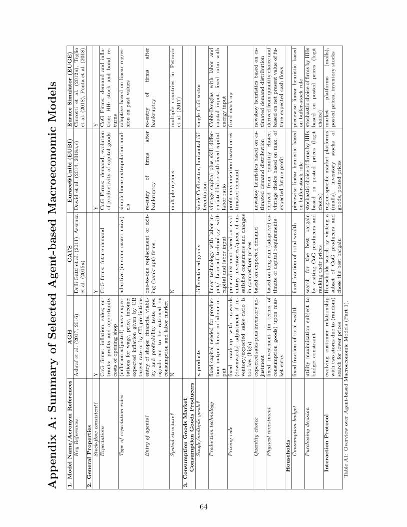
App

endix

A:

Sum

mary

of

Sele

cted

Agent-

base

dM

acr

oeco

nom

icM

odels

1.M

odelNam

e/Acronym

References

AGH

CATS

Eurace@Unib

i(E

UBI)

EuraceSim

ulato

r(E

UGE)

Key

Ref

eren

ces

Ash

raf

etal.

(2017,

2016)

Del

liG

att

iet

al.

(2011),

Ass

enza

etal.

(2015a)

Daw

idet

al.

(2014,

2018a,c

)C

inco

tti

etal.

(2012a),

Teg

lio

etal.

(2018),

Ponta

etal.

(2018)

2.GeneralProperties

Sto

ck-fl

ow

con

sist

ent?

YY

YY

Exp

ecta

tio

ns

CoG

firm

s:in

flati

on

,sa

les;

en-

trants

:p

rofi

tsan

dop

port

un

ity

cost

sof

op

enin

gsh

op

CoG

firm

s:fu

ture

dem

an

dC

oG

Fir

ms:

dem

an

d,

evolu

tion

of

pro

duct

ivit

yof

cap

ital

good

sC

oG

Fir

ms:

dem

an

dan

din

fla-

tion

;H

H:

stock

an

db

on

dre

-tu

rns

Type

of

expe

cta

tio

nru

les

(in

flati

on

ad

just

ed)

naiv

eex

pec

-ta

tion

sfo

rw

age,

pri

ce,

inco

me;

exp

ecte

din

flati

on

giv

enby

CB

targ

etra

teor

by

CB

pre

dic

tion

s

ad

ap

tive

(in

som

eca

ses:

naiv

e)si

mp

lelin

ear

extr

ap

ola

tion

mod

-el

sad

ap

tive

base

don

lin

ear

regre

s-si

on

on

past

valu

es

En

try

of

age

nts

?en

try

of

shop

s:fi

nan

cial

via

bil-

ity

an

dp

rofi

tab

ilit

yte

sts,

pos.

sign

als

not

tob

era

tion

edon

con

sum

pti

on

an

dla

bor

mark

et

on

e-to

-on

ere

pla

cem

ent

of

exit

-in

g(b

an

kru

pt)

firm

sre

-entr

yof

firm

saft

erb

an

kru

ptc

yre

-entr

yof

firm

saft

erb

an

kru

ptc

y

Spa

tia

lst

ruct

ure

?N

Nm

ult

iple

regio

ns

mu

ltip

leco

untr

ies

inP

etro

vic

etal.

(2017)

3.Consu

mption

GoodsM

arket

Consu

mption

GoodsProducers

Sin

gle/

mu

ltip

lego

ods?

np

rod

uct

sd

iffer

enti

ate

dgood

ssi

ngle

CoG

sect

or,

hori

zonta

ld

if-

fere

nti

ati

on

sin

gle

CoG

sect

or

Pro

du

ctio

nte

chn

olo

gyfi

xed

cap

ital

nee

ded

for

pro

du

c-ti

on

;ou

tpu

tlin

ear

inla

bou

rin

-p

ut

lin

ear

tech

nolo

gy

wit

hla

bor

in-

pu

t/L

eonti

efte

chn

olo

gy

wit

hca

pit

al

an

dla

bor

inp

ut

vin

tage

cap

ital

plu

ssk

ill

diff

er-

enti

ate

dla

bor

wit

hfi

xed

cap

ital-

lab

or

rati

o

Cob

b-D

ou

gla

sw

ith

lab

or

an

dca

pit

al

inp

ut,

fixed

rati

ow

ith

ener

gy

inp

ut

Pri

cin

gru

lefi

xed

mark

-up

wit

hu

pw

ard

s(d

ow

nw

ard

s)ad

just

men

tif

in-

ven

tory

/ex

pec

ted

sale

sra

tio

isto

olo

w(h

igh

)

pri

cead

just

men

tb

ase

don

invol-

unta

ryin

ven

tori

es/qu

eue

of

un

-sa

tisfi

edco

nsu

mer

san

dch

an

ges

inco

mp

etit

ors

pri

ces

pro

fit

maxim

izati

on

base

don

es-

tim

ate

dd

eman

dfi

xed

mark

-up

Qu

an

tity

cho

ice

exp

ecte

dsa

les

plu

sin

ven

tory

ad

-ju

stm

ent

base

don

exp

ecte

dd

eman

dn

ewsb

oy

heu

rist

ics

base

don

es-

tim

ate

dd

eman

dd

istr

ibu

tion

new

sboy

heu

rist

ics

base

don

es-

tim

ate

dd

eman

dd

istr

ibu

tion

Ph

ysi

cal

inve

stm

ent

fixed

inves

tmen

t(i

nte

rms

of

con

sum

pti

on

good

s)u

pon

mar-

ket

entr

y

base

don

lon

gru

n(a

dap

tive)

es-

tim

ate

of

cap

ital

requ

irem

ents

der

ived

from

qu

anti

tych

oic

e,vin

tage

choic

eb

ase

don

max.

of

exp

ecte

dfu

ture

pro

fit

der

ived

from

qu

anti

tych

oic

ean

db

ase

don

net

pre

sent

valu

eof

fu-

ture

exp

ecte

dca

shfl

ow

sHouse

hold

sC

on

sum

pti

on

bud

get

fixed

fract

ion

of

tota

lw

ealt

hfi

xed

fract

ion

of

tota

lw

ealt

hp

iece

wis

elin

ear

heu

rist

icb

ase

don

bu

ffer

-sto

ckru

lep

iece

wis

elin

ear

heu

rist

icb

ase

don

bu

ffer

-sto

ckru

leP

urc

ha

sin

gd

ecis

ion

uti

lity

maxim

izati

on

sub

ject

tob

ud

get

con

stra

int

searc

hfo

rth

eb

est

barg

ain

by

vis

itin

gC

oG

pro

du

cers

an

dra

nkin

gth

eir

pri

ces

stoch

ast

icch

oic

eoffi

rms

by

HH

sb

ase

don

post

edp

rice

s(l

ogit

choic

e)

stoch

ast

icch

oic

eoffi

rms

by

HH

sb

ase

don

post

edp

rice

s(l

ogit

choic

e)In

teraction

Proto

col

evolv

ing

cust

om

erre

lati

on

ship

wit

htw

ost

ore

sd

ue

to(r

an

dom

)se

arc

hfo

rlo

wer

pri

ces

Hou

seh

old

sse

arc

hby

vis

itin

ga

sub

set

of

CoG

pro

du

cers

an

dch

ose

the

bes

tb

arg

ain

regio

n-s

pec

ific

mark

etp

latf

orm

s(m

alls)

,in

ven

tory

stock

sof

good

s,p

ost

edp

rice

s

mark

etp

latf

orm

s(m

all

s),

post

edp

rice

s,in

ven

tory

stock

s

Tab

leA

1:

Over

vie

wover

Agen

t-b

ase

dM

acr

oec

on

om

icM

od

els

(Part

1).

64

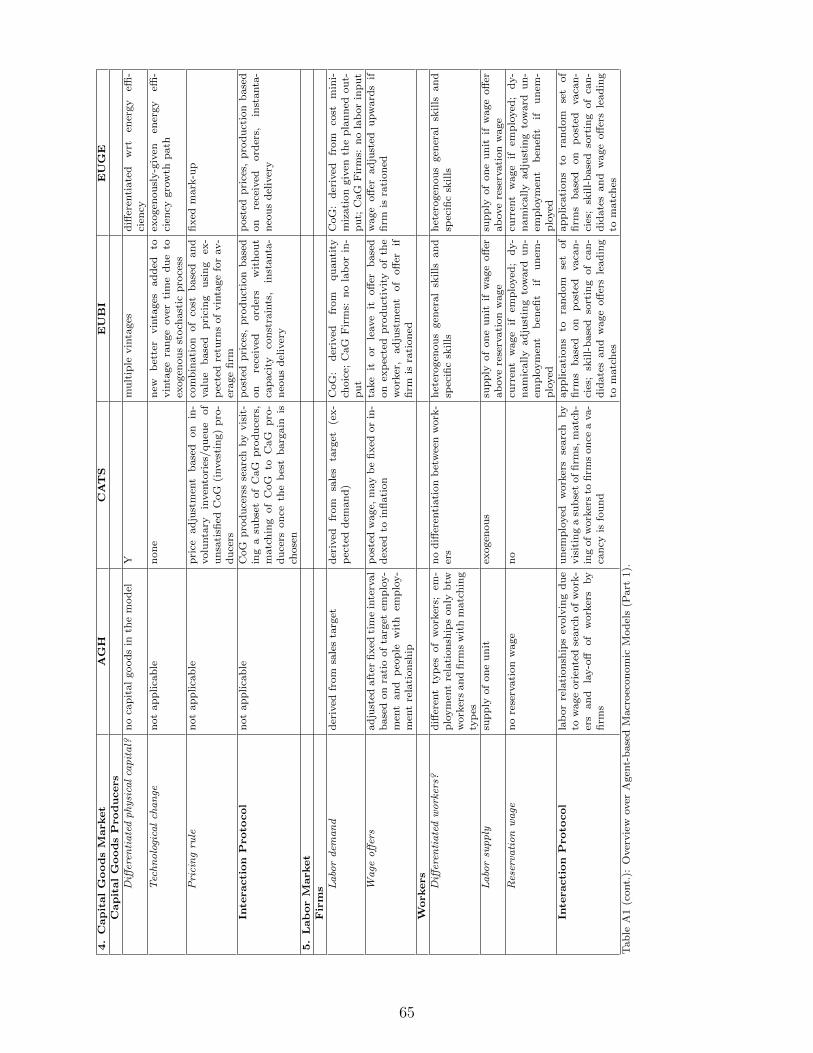
4.CapitalGoodsM

arket

AGH

CATS

EUBI

EUGE

CapitalGoodsProducers

Diff

eren

tia

ted

ph

ysi

cal

cap

ita

l?n

oca

pit

al

good

sin

the

mod

elY

mu

ltip

levin

tages

diff

eren

tiate

dw

rten

ergy

effi-

cien

cyT

ech

no

logi

cal

cha

nge

not

ap

plica

ble

non

en

ewb

ette

rvin

tages

ad

ded

tovin

tage

ran

ge

over

tim

ed

ue

toex

ogen

ou

sst

och

ast

icp

roce

ss

exogen

ou

sly-g

iven

ener

gy

effi-

cien

cygro

wth

path

Pri

cin

gru

len

ot

ap

plica

ble

pri

cead

just

men

tb

ase

don

in-

volu

nta

ryin

ven

tori

es/qu

eue

of

un

sati

sfied

CoG

(inves

tin

g)

pro

-d

uce

rs

com

bin

ati

on

of

cost

base

dan

dvalu

eb

ase

dp

rici

ng

usi

ng

ex-

pec

ted

retu

rns

of

vin

tage

for

av-

erage

firm

fixed

mark

-up

Inte

raction

Proto

col

not

ap

plica

ble

CoG

pro

du

cers

sse

arc

hby

vis

it-

ing

asu

bse

tof

CaG

pro

du

cers

,m

atc

hin

gof

CoG

toC

aG

pro

-d

uce

rson

ceth

eb

est

barg

ain

isch

ose

n

post

edp

rice

s,p

rod

uct

ion

base

don

rece

ived

ord

ers

wit

hou

tca

paci

tyco

nst

rain

ts,

inst

anta

-n

eou

sd

eliv

ery

post

edp

rice

s,p

rod

uct

ion

base

don

rece

ived

ord

ers,

inst

anta

-n

eou

sd

eliv

ery

5.LaborM

arket

Firm

s La

bor

dem

an

dd

eriv

edfr

om

sale

sta

rget

der

ived

from

sale

sta

rget

(ex-

pec

ted

dem

an

d)

CoG

:d

eriv

edfr

om

qu

anti

tych

oic

e;C

aG

Fir

ms:

no

lab

or

in-

pu

t

CoG

:d

eriv

edfr

om

cost

min

i-m

izati

on

giv

enth

ep

lan

ned

ou

t-p

ut;

CaG

Fir

ms:

no

lab

or

inp

ut

Wa

geo

ffer

sad

just

edaft

erfi

xed

tim

ein

terv

al

base

don

rati

oof

targ

etem

plo

y-

men

tan

dp

eop

lew

ith

emp

loy-

men

tre

lati

on

ship

post

edw

age,

may

be

fixed

or

in-

dex

edto

infl

ati

on

take

itor

leave

itoff

erb

ase

don

exp

ecte

dp

rod

uct

ivit

yof

the

work

er,

ad

just

men

tof

off

erif

firm

isra

tion

ed

wage

off

erad

just

edu

pw

ard

sif

firm

isra

tion

ed

Workers

Diff

eren

tia

ted

wo

rker

s?d

iffer

ent

typ

esof

work

ers;

em-

plo

ym

ent

rela

tion

ship

son

lyb

tww

ork

ers

an

dfi

rms

wit

hm

atc

hin

gty

pes

no

diff

eren

tiati

on

bet

wee

nw

ork

-er

sh

eter

ogen

ou

sgen

eral

skills

an

dsp

ecifi

csk

ills

het

erogen

ou

sgen

eral

skills

an

dsp

ecifi

csk

ills

La

bor

sup

ply

sup

ply

of

on

eu

nit

exogen

ou

ssu

pp

lyof

on

eu

nit

ifw

age

off

erab

ove

rese

rvati

on

wage

sup

ply

of

on

eu

nit

ifw

age

off

erab

ove

rese

rvati

on

wage

Res

erva

tio

nw

age

no

rese

rvati

on

wage

no

curr

ent

wage

ifem

plo

yed

;d

y-

nam

ically

ad

just

ing

tow

ard

un

-em

plo

ym

ent

ben

efit

ifu

nem

-p

loyed

curr

ent

wage

ifem

plo

yed

;d

y-

nam

ically

ad

just

ing

tow

ard

un

-em

plo

ym

ent

ben

efit

ifu

nem

-p

loyed

Inte

raction

Proto

col

lab

or

rela

tion

ship

sev

olv

ing

du

eto

wage

ori

ente

dse

arc

hof

work

-er

san

dla

y-o

ffof

work

ers

by

firm

s

un

emp

loyed

work

ers

searc

hby

vis

itin

ga

sub

set

of

firm

s,m

atc

h-

ing

of

work

ers

tofi

rms

on

cea

va-

can

cyis

fou

nd

ap

plica

tion

sto

ran

dom

set

of

firm

sb

ase

don

post

edvaca

n-

cies

;sk

ill-

base

dso

rtin

gof

can

-d

idate

san

dw

age

off

ers

lead

ing

tom

atc

hes

ap

plica

tion

sto

ran

dom

set

of

firm

sb

ase

don

post

edvaca

n-

cies

;sk

ill-

base

dso

rtin

gof

can

-d

idate

san

dw

age

off

ers

lead

ing

tom

atc

hes

Tab

leA

1(c

ont.

):O

ver

vie

wover

Agen

t-b

ase

dM

acr

oec

on

om

icM

od

els

(Part

1).

65

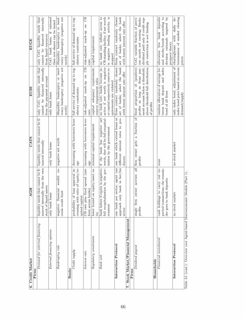
6.Credit

Market

AGH

CATS

EUBI

EUGE

Firm

s Dem

an

dfo

rex

tern

al

fin

an

cin

gliqu

idit

yn

eed

sth

at

can

not

be

fi-

nan

ced

inte

rnally

from

the

ow

nst

ock

of

liqu

idass

ets

liqu

idit

yn

eed

sth

at

can

not

be

fi-

nan

ced

inte

rnally

on

lyC

oG

:liqu

idit

yn

eed

sth

at

can

not

be

fin

an

ced

inte

rnally

from

the

paym

ent

acc

ou

nt

on

lyC

oG

:liqu

idit

yn

eed

sth

at

can

not

be

fin

an

ced

inte

rnally

from

liqu

idre

sou

rces

Ext

ern

al

fin

an

cin

go

pti

on

son

lyb

an

klo

an

son

lyb

an

klo

an

son

lyb

an

klo

an

sC

oG

:b

an

klo

an

s,if

rati

on

edth

enn

ewsh

are

sca

nb

eis

sued

Ba

nkr

up

tcy

rule

neg

ati

ve

fin

an

cial

wea

lth

ex-

ceed

scr

edit

lim

itn

egati

ve

net

wort

hilliqu

idit

yb

an

kru

ptc

yor

inso

l-ven

cyb

an

kru

ptc

y(n

egati

ve

net

wort

h)

illiqu

idit

yb

an

kru

ptc

yor

inso

l-ven

cyb

an

kru

ptc

y(n

egati

ve

net

wort

h)

Banks C

red

itsu

pp

lyp

rob

ab

ilit

yof

loan

ap

pro

val

in-

crea

sin

gw

ith

rati

oof

equ

ity/re

-qu

ired

cap

ital

dec

reasi

ng

wit

hb

orr

ow

ers

lever

-age

full

serv

ice

of

dem

an

du

pto

reg-

ula

tory

con

stra

ints

full

serv

ice

of

dem

an

du

pto

reg-

ula

tory

con

stra

ints

Inte

rest

rate

CB

rate

plu

sfi

xed

spre

ad

(un

i-fo

rmacr

oss

ban

ks)

incr

easi

ng

wit

hb

orr

ow

ers

lever

-age

risk

-ad

just

edm

ark

-up

on

CB

rate

risk

-ad

just

edm

ark

-up

on

CB

rate

Reg

ula

tory

con

stra

ints

low

erb

ou

nd

on

equ

ity/ass

etra

-ti

om

inim

al

cap

ital

requ

irem

ent

cap

ital

ad

equ

acy

requ

irem

ent;

rese

rve

requ

irem

ent

rati

oca

pit

al

requ

irem

ent

Ba

nk

exit

ban

kfa

ilu

reif

equ

ity

isn

egati

ve;

full

reca

pit

aliza

tion

by

the

gov-

ern

men

t

ifth

eb

an

kh

as

neg

ati

ve

net

wort

h,

ther

willb

efu

llre

cpait

al-

izati

on

by

the

gover

nm

ent

no

ban

kex

it;

ban

ks

bec

om

ein

-act

ive

ifn

etw

ort

his

neg

ati

ve

or

cap

tialre

spec

tivel

yre

serv

ere

-qu

irem

ents

are

vio

late

d

no

ban

kex

it;

infi

nit

eacc

ess

toC

Bst

an

din

gfa

cility

;if

net

wort

his

neg

ati

ve

len

din

gact

ivit

yis

stop

ped

Inte

raction

Proto

col

on

eb

an

kp

erse

ctor;

agen

tca

nap

pro

ach

on

lyb

an

kin

her

/h

isse

ctor

on

eb

an

kw

hic

hex

ten

dlo

an

sat

diff

eren

tin

tere

stra

tes

top

ro-

du

cers

firm

sco

nta

ctra

nd

om

lych

ose

nse

tof

ban

ks;

sele

ctth

eb

an

kw

ith

low

est

inte

rest

rate

off

er

firm

sco

nta

ctra

nd

om

lych

ose

nse

tof

ban

ks;

sele

ctth

eb

an

kw

ith

low

est

inte

rest

rate

off

er7.Sto

ck

Market/

Fin

ancialM

anagem

ent

Firm

s Div

iden

dpa

yo

ut

sin

gle

firm

ow

ner

acc

rues

all

pro

fits

firm

ow

ner

get

sa

fract

ion

of

pro

fits

fixed

pro

port

ion

of

(posi

tive)

pro

fits

as

lon

gas

firm

sp

ay-

men

tacc

ou

nt

bel

ow

ath

resh

old

,ab

ove

thre

shold

full

dis

trib

uti

on

of

pro

fits

CoG

:vari

ab

lefr

act

ion

of

pre

vi-

ou

sm

onth

net

earn

ing;

Ban

ks:

div

iden

dp

aid

on

lyif

cred

itsu

p-

ply

rest

rict

ion

isn

ot

bin

din

g

House

hold

sF

ina

nci

al

inve

stm

ent

cash

hold

ings

toca

rry

ou

tex

-p

ecte

dtr

an

sact

ion

s,th

ere

main

-d

ergoes

tob

an

kd

eposi

ts

non

era

nd

om

alloca

tion

of

savin

gs

be-

twee

nb

an

kd

eposi

tan

din

dex

bon

dof

all

firm

s

alloca

tion

btw

ban

kd

eposi

tsan

dst

ock

s/b

on

ds

acc

ord

ing

tod

ecis

ion

rati

on

ale

insp

ired

by

pro

spec

tth

eory

Inte

raction

Proto

col

no

stock

mark

etn

ost

ock

mark

eton

lyin

dex

bon

d,

ad

just

men

tof

ind

exb

on

dp

rice

base

don

exce

ssd

eman

d/su

pp

ly

clea

rin

gh

ou

sew

ith

daily

de-

term

inati

on

of

mark

etcl

eari

ng

pri

ces

Tab

leA

1(c

ont.

):O

ver

vie

wover

Agen

t-b

ase

dM

acr

oec

on

om

icM

od

els

(Part

1).

66

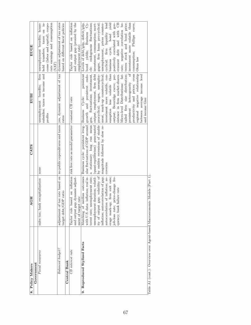
8.Policy

Makers

AGH

CATS

EUBI

EUGE

Governm

ent

Fis

cal

mea

sure

ssa

les

tax;

ban

kre

cap

itali

zati

on

non

eu

nem

plo

ym

ent

ben

efits

;fi

rmsu

bsi

die

s;ta

xes

on

inco

me

an

dp

rofi

ts

un

emp

loym

ent

ben

efits

;h

ou

se-

hold

tran

sfer

s;ta

xes

on

in-

com

e(l

ab

or

an

dca

pit

al)

,co

rpo-

rate

earn

ings

an

dco

nsu

mp

tion

(VA

T)

Ba

lan

ced

bud

get?

ad

just

men

tof

tax

rate

base

don

targ

etd

ebt/

GD

Pra

tio

no

pu

blic

exp

end

itu

res

an

dta

xes

yes

,d

yn

am

icad

just

men

tof

tax

rate

sd

yn

am

icad

just

men

tof

tax

rate

sb

ase

don

diff

eren

tfi

scal

polici

esCentralBank

CB

inte

rest

rate

Taylo

rru

leb

ase

don

infl

ati

on

an

dou

tpu

tgap

;d

yn

am

icad

just

-m

ent

of

targ

etra

te

risk

free

rate

as

mod

elp

ara

met

erco

nst

ant

CB

rate

Taylo

rru

leb

ase

don

infl

ati

on

an

dou

tpu

tgap

(pro

xie

dby

the

emp

loym

ent

rate

)9.Reproduced

Sty

lized

Facts

Matc

hin

gof

med

ian

ou

tcom

esw

ith

U.S

.d

ata

:in

flati

on

;re

alin

-te

rest

rate

;u

nem

plo

ym

ent

rate

;u

nem

plo

ym

ent

du

rati

on

;vola

til-

ity

of

ou

tpu

tgap

;vola

tility

of

infl

ati

on

;au

toco

rrel

ati

on

of

gap

;au

toco

rrel

ati

on

of

infl

ati

on

;av-

erage

mark

-up

;fi

rmex

itra

te;

job

-loss

rate

;p

rice

-ch

an

ge

fre-

qu

ency

;b

an

kfa

ilu

rera

te

Bu

sin

ess

cycl

e:p

ersi

sten

tir

reg-

ula

rfl

uct

uati

on

sof

GD

Paro

un

da

stati

on

ary

lon

gru

nm

ean

(qu

asi

-equ

ilib

riu

m)

pu

nct

uate

dby

sud

den

rece

ssio

ns

of

siza

ble

magn

itu

de

follow

edby

slow

re-

cover

ies

Bu

sin

ess

Cycl

e:p

ersi

sten

tgro

wth

an

dp

ersi

sten

ten

do-

gen

.fl

uct

uati

on

s;in

ves

tmen

t,ou

tpu

t,em

plo

ym

ent,

firm

deb

tp

rocy

clic

al;

wages

,u

nem

plo

y-

men

t,m

ark

-up

cou

nte

rcycl

ical;

inves

tmen

tm

ore

vola

tile

,co

n-

sum

pti

on

less

vola

tile

than

ou

tpu

t;B

ever

idge

curv

e;p

er-

sist

ence

infi

rmm

ark

et-s

hare

s.M

icro

-lev

elD

istr

ibu

tion

s:fa

t-ta

iled

firm

size

dis

trib

uti

on

;p

ersi

sten

th

eter

ogen

eity

of

pro

du

ctiv

ity

an

dp

rice

s;cr

oss

regio

nal

neg

ati

ve

rela

tion

ship

bet

wee

naver

age

inco

me

level

an

din

com

eG

ini

Lev

els

of

deb

t/gd

p,

defi

cit/

gd

p,

bon

dyie

lds;

Bu

sin

ess

Cy-

cle:

end

ogen

ou

sfl

uct

uati

on

s;in

ves

tmen

t,co

nsu

mp

tion

;m

ort

-gages

,fi

rmlo

an

sp

ro-c

ycl

ical;

un

emp

loym

ent,

pri

ces

cou

nte

r-cy

clic

al;

firm

liqu

idit

yle

ad

bu

sin

ess

cycl

e;b

on

dyie

ldp

osi

tivel

yco

rrel

ate

dw

ith

gov-

ern

men

td

ebt

an

dw

ith

CB

rate

;n

egati

ve

corr

elati

on

be-

twee

nst

ock

an

db

on

dp

rice

;in

ves

tmen

tm

ore

vola

tile

than

con

sum

pti

on

;P

hillip

scu

rve,

Oku

nla

w

Tab

leA

1(c

ont.

):O

ver

vie

wover

Agen

t-b

ase

dM

acr

oec

on

om

icM

od

els

(Part

1).

67

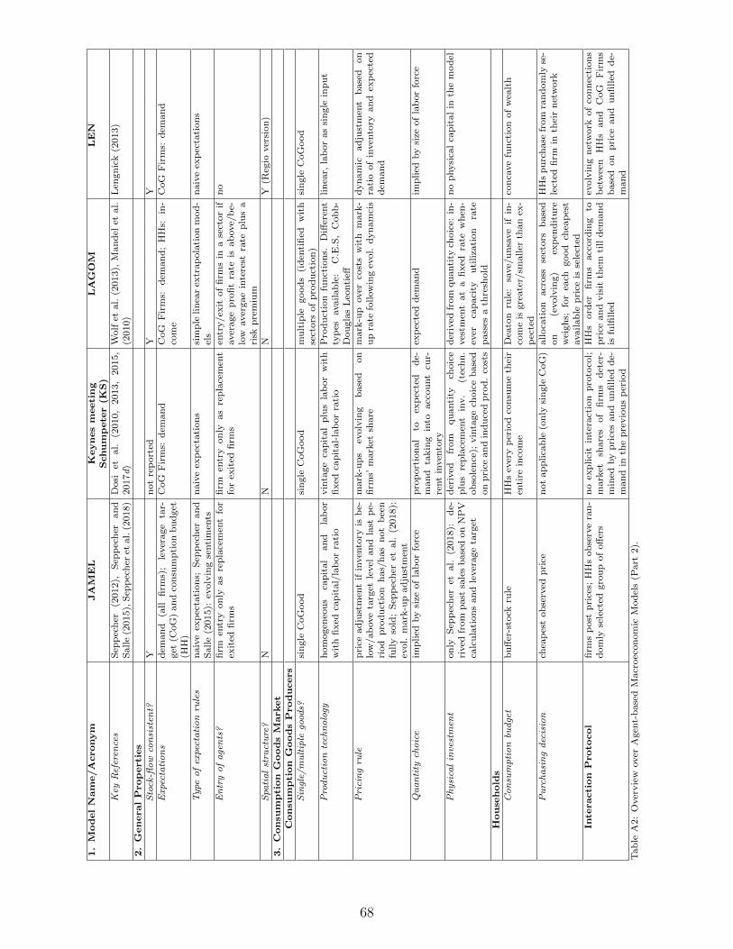
1.M

odelNam

e/Acronym

JAM

EL

Keynesm

eeting

Schum

pete

r(K

S)

LAGOM

LEN

Key

Ref

eren

ces

Sep

pec

her

(2012),

Sep

pec

her

an

dS

alle

(2015),

Sep

pec

her

etal.

(2018)

Dosi

etal.

(2010,

2013,

2015,

2017d)

Wolf

etal.

(2013),

Man

del

etal.

(2010)

Len

gn

ick

(2013)

2.GeneralProperties

Sto

ck-fl

ow

con

sist

ent?

Yn

ot

rep

ort

edY

YE

xpec

tati

on

sd

eman

d(a

llfi

rms)

;le

ver

age

tar-

get

(CoG

)an

dco

nsu

mp

tion

bu

dget

(HH

)

CoG

Fir

ms:

dem

an

dC

oG

Fir

ms:

dem

an

d;

HH

s:in

-co

me

CoG

Fir

ms:

dem

an

d

Type

of

expe

cta

tio

nru

les

naiv

eex

pec

tati

on

s;S

epp

ech

eran

dS

alle

(2015):

evolv

ing

senti

men

tsn

aiv

eex

pec

tati

on

ssi

mp

lelin

ear

extr

ap

ola

tion

mod

-el

sn

aiv

eex

pec

tati

on

s

En

try

of

age

nts

?fi

rmen

try

on

lyas

repla

cem

ent

for

exit

edfi

rms

firm

entr

yon

lyas

rep

lace

men

tfo

rex

ited

firm

sen

try/ex

itof

firm

sin

ase

ctor

ifaver

age

pro

fit

rate

isab

ove/

be-

low

aver

gae

inte

rest

rate

plu

sa

risk

pre

miu

m

no

Spa

tia

lst

ruct

ure

?N

NN

Y(R

egio

ver

sion

)3.Consu

mption

GoodsM

arket

Consu

mption

GoodsProducers

Sin

gle/

mu

ltip

lego

ods?

sin

gle

CoG

ood

sin

gle

CoG

ood

mu

ltip

legood

s(i

den

tifi

edw

ith

sect

ors

of

pro

du

ctio

n)

sin

gle

CoG

ood

Pro

du

ctio

nte

chn

olo

gyh

om

ogen

eou

sca

pit

al

an

dla

bor

wit

hfi

xed

cap

ital/

lab

or

rati

ovin

tage

cap

ital

plu

sla

bor

wit

hfi

xed

cap

ital-

lab

or

rati

oP

rod

uct

ion

fun

ctio

ns.

Diff

eren

tty

pes

availab

le:

C.E

.S,

Cob

b-

Dou

gla

sL

eonti

eff

lin

ear,

lab

or

as

sin

gle

inp

ut

Pri

cin

gru

lep

rice

ad

just

men

tif

inven

tory

isb

e-lo

w/ab

ove

targ

etle

vel

an

dla

stp

e-ri

od

pro

du

ctio

nh

as/

has

not

bee

nfu

lly

sold

;S

epp

ech

eret

al.

(2018):

evol.

mark

-up

ad

just

men

t

mark

-up

sev

olv

ing

base

don

firm

s’m

ark

etsh

are

mark

-up

over

cost

sw

ith

mark

-u

pra

tefo

llow

ing

evol.

dyn

am

cis

dyn

am

icad

just

men

tb

ase

don

rati

oof

inven

tory

an

dex

pec

ted

dem

an

d

Qu

an

tity

cho

ice

imp

lied

by

size

of

lab

or

forc

ep

rop

ort

ion

al

toex

pec

ted

de-

man

dta

kin

gin

toacc

ou

nt

cur-

rent

inven

tory

exp

ecte

dd

eman

dim

plied

by

size

of

lab

or

forc

e

Ph

ysi

cal

inve

stm

ent

on

lyS

epp

ech

eret

al.

(2018):

de-

rived

from

past

sale

sb

ase

don

NP

Vca

lcu

lati

on

san

dle

ver

age

targ

et

der

ived

from

qu

anti

tych

oic

ep

lus

rep

lace

men

tin

v.

(tec

hn

.ob

sole

nce

);vin

tage

choic

eb

ase

don

pri

cean

din

du

ced

pro

d.

cost

s

der

ived

from

qu

anti

tych

oic

e:in

-ves

tmen

tat

afixed

rate

wh

en-

ever

cap

aci

tyu

tiliza

tion

rate

pass

esa

thre

shold

no

physi

cal

cap

ital

inth

em

od

el

House

hold

sC

on

sum

pti

on

bud

get

bu

ffer

-sto

ckru

leH

Hs

ever

yp

erio

dco

nsu

me

thei

ren

tire

inco

me

Dea

ton

rule

:sa

ve/

un

save

ifin

-co

me

isgre

ate

r/sm

aller

than

ex-

pec

ted

con

cave

fun

ctio

nof

wea

lth

Pu

rch

asi

ng

dec

isio

nch

eap

est

ob

serv

edp

rice

not

ap

plica

ble

(on

lysi

ngle

CoG

)alloca

tion

acr

oss

sect

ors

base

don

(evolv

ing)

exp

end

itu

rew

eigh

s;fo

rea

chgood

chea

pes

tavailab

lep

rice

isse

lect

ed

HH

sp

urc

hase

from

ran

dom

lyse

-le

cted

firm

inth

eir

net

work

Inte

raction

Proto

col

firm

sp

ost

pri

ces;

HH

sob

serv

era

n-

dom

lyse

lect

edgro

up

of

off

ers

no

exp

lici

tin

tera

ctio

np

roto

col;

mark

etsh

are

sof

firm

sd

eter

-m

ined

by

pri

ces

an

dun

fill

edd

e-m

an

din

the

pre

vio

us

per

iod

HH

sord

erfi

rms

acc

ord

ing

top

rice

an

dvis

itth

emti

lld

eman

dis

fulfi

lled

evolv

ing

net

work

of

con

nec

tion

sb

etw

een

HH

san

dC

oG

Fir

ms

base

don

pri

cean

du

nfi

lled

de-

man

d

Tab

leA

2:

Over

vie

wover

Agen

t-b

ase

dM

acr

oec

on

om

icM

od

els

(Part

2).

68

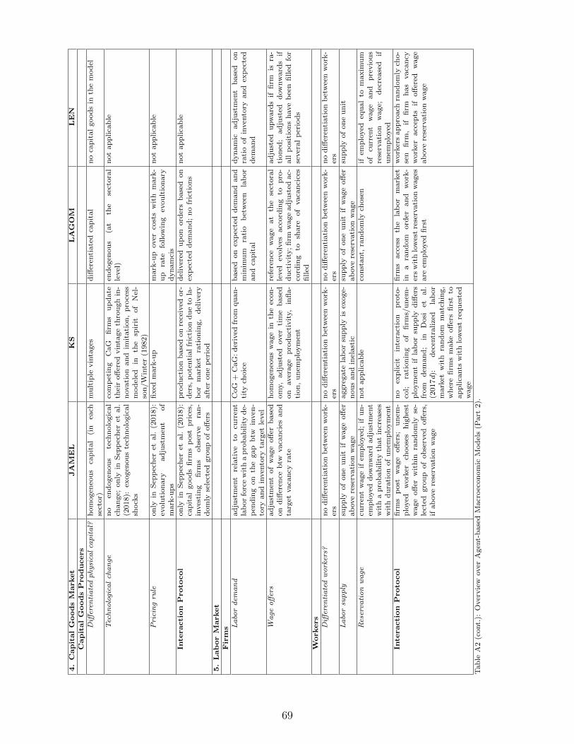
4.CapitalGoodsM

arket

JAM

EL

KS

LAGOM

LEN

CapitalGoodsProducers

Diff

eren

tia

ted

ph

ysi

cal

cap

ita

l?h

om

ogen

eou

sca

pit

al

(in

each

sect

or)

mult

iple

vin

tages

diff

eren

tiate

dca

pit

al

no

cap

ital

good

sin

the

mod

el

Tec

hn

olo

gica

lch

an

gen

oen

dogen

ou

ste

chn

olo

gic

al

change;

on

lyin

Sep

pec

her

etal.

(2018):

exogen

ou

ste

chn

olo

gic

al

shock

s

com

pet

ing

CaG

firm

su

pd

ate

thei

roff

ered

vin

tage

thro

ugh

in-

novati

on

an

dim

itati

on

,p

roce

ssm

od

eled

inth

esp

irit

of

Nel

-so

n/W

inte

r(1

982)

end

ogen

ou

s(a

tth

ese

ctora

lle

vel

)n

ot

ap

plica

ble

Pri

cin

gru

leon

lyin

Sep

pec

her

etal.

(2018):

evolu

tion

ary

ad

just

men

tof

mark

-up

s

fixed

mark

-up

mark

-up

over

cost

sw

ith

mark

-u

pra

tefo

llow

ing

evou

ltio

nary

dyn

am

cis

not

ap

plica

ble

Inte

raction

Proto

col

on

lyin

Sep

pec

her

etal.

(2018):

cap

ital

good

sfi

rms

post

pri

ces,

inves

tin

gfi

rms

ob

serv

era

n-

dom

lyse

lect

edgro

up

of

off

ers

pro

du

ctio

nb

ase

don

rece

ived

or-

der

s,p

ote

nti

al

fric

tion

du

eto

la-

bor

mark

etra

tion

ing,

del

iver

yaft

eron

ep

erio

d

del

iver

edu

pon

ord

ers

base

don

exp

ecte

dd

eman

d;

no

fric

tion

sn

ot

ap

plica

ble

5.LaborM

arket

Firm

s La

bor

dem

an

dad

just

men

tre

lati

ve

tocu

rren

tla

bor

forc

ew

ith

ap

rob

ab

ilit

yd

e-p

end

ing

on

the

gap

btw

inven

-to

ryan

din

ven

tory

targ

etle

vel

CoG

+C

aG

:d

eriv

edfr

om

qu

an

-ti

tych

oic

eb

ase

don

exp

ecte

dd

eman

dan

dm

inim

um

rati

ob

etw

een

lab

or

an

dca

pit

al

dyn

am

icad

just

men

tb

ase

don

rati

oof

inven

tory

an

dex

pec

ted

dem

an

d

Wa

geo

ffer

sad

just

men

tof

wage

off

erb

ase

don

diff

eren

ceb

twvaca

nci

esan

dta

rget

vaca

ncy

rate

hom

ogen

eou

sw

age

inth

eec

on

-om

y,ad

just

edover

tim

eb

ase

don

aver

age

pro

du

ctiv

ity,

infl

a-

tion

,u

nem

plo

ym

ent

refe

ren

cew

age

at

the

sect

ora

lle

vel

evolv

esacc

ord

ing

top

ro-

du

ctiv

ity;fi

rmw

age

ad

just

edac-

cord

ing

tosh

are

of

vaca

nci

ces

filled

ad

just

edu

pw

ard

sif

firm

isra

-ti

on

ed;

ad

just

edd

ow

nw

ard

sif

all

posi

tion

sh

ave

bee

nfi

lled

for

sever

al

per

iod

s

Workers

Diff

eren

tia

ted

wo

rker

s?n

od

iffer

enti

ati

on

bet

wee

nw

ork

-er

sn

od

iffer

enti

ati

on

bet

wee

nw

ork

-er

sn

od

iffer

enti

ati

on

bet

wee

nw

ork

-er

sn

od

iffer

enti

ati

on

bet

wee

nw

ork

-er

sL

abo

rsu

pp

lysu

pp

lyof

on

eu

nit

ifw

age

off

erab

ove

rese

rvati

on

wage

aggre

gate

lab

or

sup

ply

isex

oge-

nou

san

din

elast

icsu

pp

lyof

on

eu

nit

ifw

age

off

erab

ove

rese

rvati

on

wage

sup

ply

of

on

eu

nit

Res

erva

tio

nw

age

curr

ent

wage

ifem

plo

yed

;if

un

-em

plo

yed

dow

nw

ard

ad

just

men

tw

ith

ap

rob

ab

ilit

yth

at

incr

ease

sw

ith

du

rati

on

of

un

emp

loym

ent

not

ap

plica

ble

con

stant,

ran

dom

lych

ose

nif

emp

loyed

equ

al

tom

axim

um

of

curr

ent

wage

an

dp

revio

us

rese

rvati

on

wage;

dec

rease

dif

un

emp

loyed

Inte

raction

Proto

col

firm

sp

ost

wage

off

ers;

un

em-

plo

yed

work

erch

oose

sh

igh

est

wage

off

erw

ith

inra

nd

om

lyse

-le

cted

gro

up

of

ob

serv

edoff

ers,

ifab

ove

rese

rvati

on

wage

no

exp

lici

tin

tera

ctio

np

roto

-co

l;ra

tion

ing

of

firm

s/u

nem

-p

loym

ent

ifla

bor

sup

ply

diff

ers

from

dem

an

d;

inD

osi

etal.

(2017d):

dec

entr

alize

dla

bor

mark

etw

ith

ran

dom

matc

hin

g,

wh

ere

firm

sm

ake

off

ers

firs

tto

ap

plica

nts

wit

hlo

wes

tre

qu

este

dw

age

firm

sacc

ess

the

lab

or

mark

etin

ara

nd

om

ord

eran

dw

ork

-er

sw

ith

low

est

rese

rvati

on

wages

are

emp

loyed

firs

t

work

ers

ap

pro

ach

ran

dom

lych

o-

sen

firm

,if

firm

has

vaca

ncy

work

eracc

epts

ifoff

ered

wage

ab

ove

rese

rvati

on

wage

Tab

leA

2(c

ont.

):O

ver

vie

wover

Agen

t-b

ase

dM

acr

oec

on

om

icM

od

els

(Part

2).

69

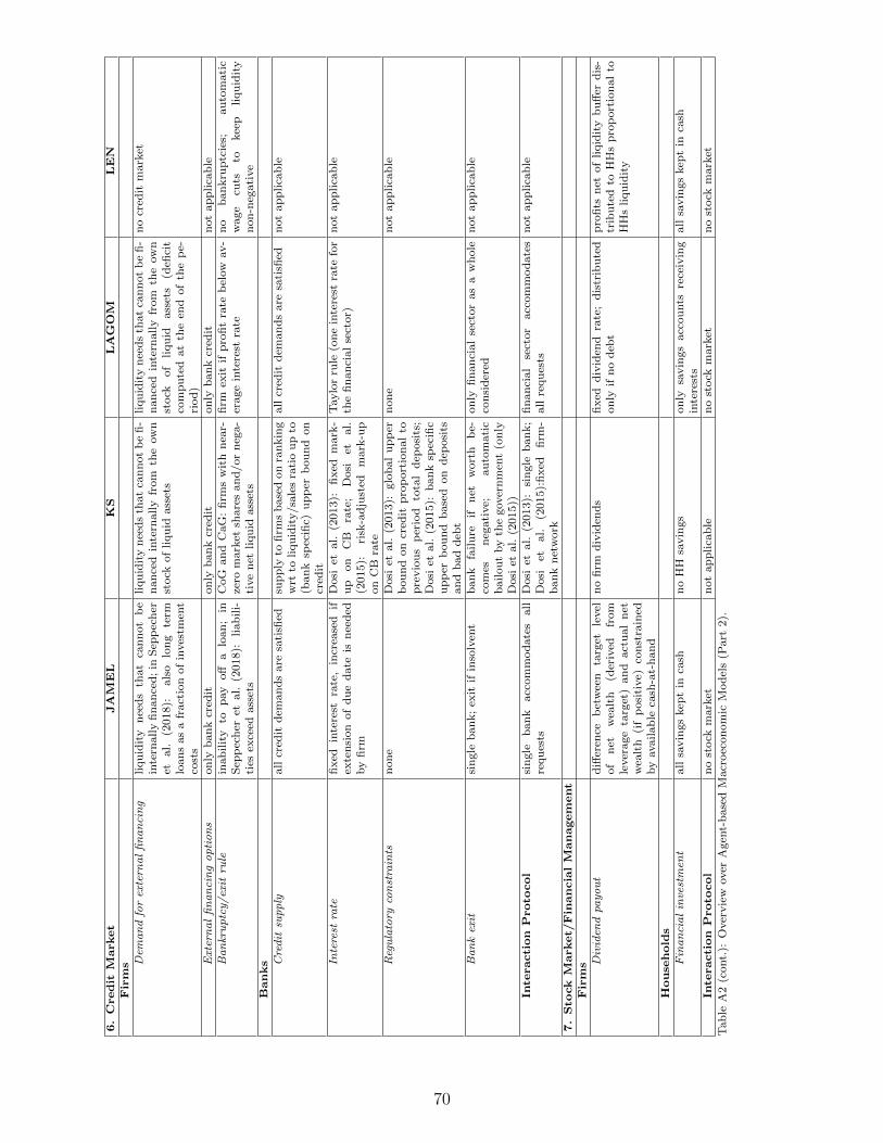
6.Credit

Market

JAM

EL

KS

LAGOM

LEN

Firm

s Dem

an

dfo

rex

tern

al

fin

an

cin

gliqu

idit

yn

eed

sth

at

can

not

be

inte

rnall

yfi

nan

ced

;in

Sep

pec

her

etal.

(2018):

als

olo

ng

term

loan

sas

afr

act

ion

of

inves

tmen

tco

sts

liqu

idit

yn

eed

sth

at

can

not

be

fi-

nan

ced

inte

rnally

from

the

ow

nst

ock

of

liqu

idass

ets

liqu

idit

yn

eed

sth

at

can

not

be

fi-

nan

ced

inte

rnally

from

the

ow

nst

ock

of

liqu

idass

ets

(defi

cit

com

pu

ted

at

the

end

of

the

pe-

riod

)

no

cred

itm

ark

et

Ext

ern

al

fin

an

cin

go

pti

on

son

lyb

an

kcr

edit

on

lyb

an

kcr

edit

on

lyb

an

kcr

edit

not

ap

plica

ble

Ba

nkr

up

tcy/

exit

rule

inab

ilit

yto

pay

off

alo

an

;in

Sep

pec

her

etal.

(2018):

liab

ili-

ties

exce

edass

ets

CoG

an

dC

aG

:fi

rms

wit

hn

ear-

zero

mark

etsh

are

san

d/or

neg

a-

tive

net

liqu

idass

ets

firm

exit

ifp

rofi

tra

teb

elow

av-

erage

inte

rest

rate

no

ban

kru

ptc

ies;

au

tom

ati

cw

age

cuts

tokee

pliqu

idit

yn

on

-neg

ati

ve

Banks C

red

itsu

pp

lyall

cred

itd

eman

ds

are

sati

sfied

sup

ply

tofi

rms

base

don

ran

kin

gw

rtto

liqu

idit

y/sa

les

rati

ou

pto

(ban

ksp

ecifi

c)u

pp

erb

ou

nd

on

cred

it

all

cred

itd

eman

ds

are

sati

sfied

not

ap

plica

ble

Inte

rest

rate

fixed

inte

rest

rate

,in

crea

sed

ifex

ten

sion

of

du

ed

ate

isn

eed

edby

firm

Dosi

etal.

(2013):

fixed

mark

-u

pon

CB

rate

;D

osi

etal.

(2015):

risk

-ad

just

edm

ark

-up

on

CB

rate

Taylo

rru

le(o

ne

inte

rest

rate

for

the

fin

an

cial

sect

or)

not

ap

plica

ble

Reg

ula

tory

con

stra

ints

non

eD

osi

etal.

(2013):

glo

bal

up

per

bou

nd

on

cred

itp

rop

ort

ion

al

top

revio

us

per

iod

tota

ld

eposi

ts;

Dosi

etal.

(2015):

ban

ksp

ecifi

cu

pp

erb

ou

nd

base

don

dep

osi

tsan

db

ad

deb

t

non

en

ot

ap

plica

ble

Ba

nk

exit

sin

gle

ban

k;

exit

ifin

solv

ent

ban

kfa

ilu

reif

net

wort

hb

e-co

mes

neg

ati

ve;

au

tom

ati

cb

ailou

tby

the

gover

nm

ent

(on

lyD

osi

etal.

(2015))

on

lyfi

nan

cial

sect

or

as

aw

hole

con

sid

ered

not

ap

plica

ble

Inte

raction

Proto

col

sin

gle

ban

kacc

om

mod

ate

sall

requ

ests

Dosi

etal.

(2013):

sin

gle

ban

k;

Dosi

etal.

(2015):

fixed

firm

-b

an

kn

etw

ork

fin

an

cial

sect

or

acc

om

mod

ate

sall

requ

ests

not

ap

plica

ble

7.Sto

ck

Market/

Fin

ancialM

anagem

ent

Firm

s Div

iden

dpa

yo

ut

diff

eren

ceb

etw

een

targ

etle

vel

of

net

wea

lth

(der

ived

from

lever

age

targ

et)

an

dact

ual

net

wea

lth

(if

posi

tive)

con

stra

ined

by

availab

leca

sh-a

t-h

an

d

no

firm

div

iden

ds

fixed

div

iden

dra

te;

dis

trib

ute

don

lyif

no

deb

tp

rofi

tsn

etof

liqid

ity

buff

erd

is-

trib

ute

dto

HH

sp

rop

ort

ion

al

toH

Hs

liqu

idit

y

House

hold

sF

ina

nci

al

inve

stm

ent

all

savin

gs

kep

tin

cash

no

HH

savin

gs

on

lysa

vin

gs

acc

ou

nts

rece

ivin

gin

tere

sts

all

savin

gs

kep

tin

cash

Inte

raction

Proto

col

no

stock

mark

etn

ot

ap

plica

ble

no

stock

mark

etn

ost

ock

mark

et

Tab

leA

2(c

ont.

):O

ver

vie

wover

Agen

t-b

ase

dM

acr

oec

on

om

icM

od

els

(Part

2).

70

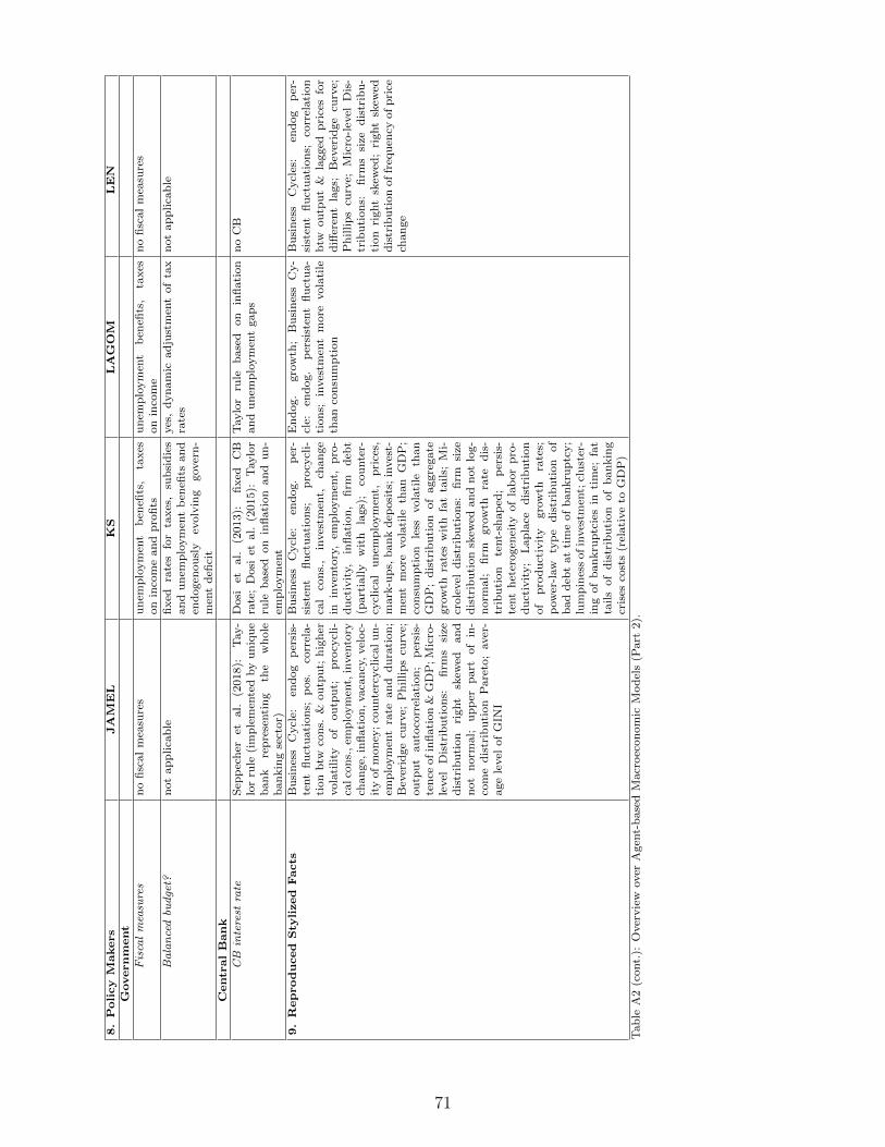
8.Policy

Makers

JAM

EL

KS

LAGOM

LEN

Governm

ent

Fis

cal

mea

sure

sn

ofi

scal

mea

sure

su

nem

plo

ym

ent

ben

efits

,ta

xes

on

inco

me

an

dp

rofi

tsu

nem

plo

ym

ent

ben

efits

,ta

xes

on

inco

me

no

fisc

al

mea

sure

s

Ba

lan

ced

bud

get?

not

ap

plica

ble

fixed

rate

sfo

rta

xes

,su

bsi

die

san

du

nem

plo

ym

ent

ben

efits

and

end

ogen

ou

sly

evolv

ing

gover

n-

men

td

efici

t

yes

,d

yn

am

icad

just

men

tof

tax

rate

sn

ot

ap

plica

ble

CentralBank

CB

inte

rest

rate

Sep

pec

her

etal.

(2018):

Tay-

lor

rule

(im

ple

men

ted

by

un

iqu

eb

an

kre

pre

senti

ng

the

wh

ole

ban

kin

gse

ctor)

Dosi

etal.

(2013):

fixed

CB

rate

;D

osi

etal.

(2015):

Taylo

rru

leb

ase

don

infl

ati

on

an

du

n-

emp

loym

ent

Taylo

rru

leb

ase

don

infl

ati

on

an

du

nem

plo

ym

ent

gap

sn

oC

B

9.Reproduced

Sty

lized

Facts

Bu

sin

ess

Cycl

e:en

dog

per

sis-

tent

flu

ctu

ati

on

s;p

os.

corr

ela-

tion

btw

con

s.&

ou

tpu

t;h

igh

ervola

tility

of

ou

tpu

t;p

rocy

cli-

calco

ns.

,em

plo

ym

ent,

inven

tory

change,

infl

ati

on

,vaca

ncy

,vel

oc-

ity

of

mon

ey;

cou

nte

rcycl

icalu

n-

emp

loym

ent

rate

an

dd

ura

tion

;B

ever

idge

curv

e;P

hillip

scu

rve;

ou

tpu

tau

toco

rrel

ati

on

;p

ersi

s-te

nce

ofin

flati

on

&G

DP

;M

icro

-le

vel

Dis

trib

uti

on

s:fi

rms

size

dis

trib

uti

on

right

skew

edan

dn

ot

norm

al;

up

per

part

of

in-

com

ed

istr

ibu

tion

Pare

to;

aver

-age

level

of

GIN

I

Bu

sin

ess

Cycl

e:en

dog.

per

-si

sten

tfl

uct

uati

on

s;p

rocy

cli-

cal

con

s.,

inves

tmen

t,ch

an

ge

inin

ven

tory

,em

plo

ym

ent,

pro

-d

uct

ivit

y,in

flati

on

,fi

rmd

ebt

(part

ially

wit

hla

gs)

;co

unte

r-cy

clic

al

un

emp

loym

ent,

pri

ces,

mark

-up

s,b

an

kd

eposi

ts;

inves

t-m

ent

more

vola

tile

than

GD

P;

con

sum

pti

on

less

vola

tile

than

GD

P;

dis

trib

uti

on

of

aggre

gate

gro

wth

rate

sw

ith

fat

tails;

Mi-

crole

vel

dis

trib

uti

on

s:fi

rmsi

zed

istr

ibu

tion

skew

edan

dn

ot

log-

norm

al;

firm

gro

wth

rate

dis

-tr

ibu

tion

tent-

shap

ed;

per

sis-

tent

het

erogen

eity

of

lab

or

pro

-d

uct

ivit

y;

Lap

lace

dis

trib

uti

on

of

pro

du

ctiv

ity

gro

wth

rate

s;p

ow

er-l

aw

typ

ed

istr

ibu

tion

of

bad

deb

tat

tim

eof

ban

kru

ptc

y;

lum

pin

ess

ofin

ves

tmen

t;cl

ust

er-

ing

of

ban

kru

ptc

ies

inti

me;

fat

tails

of

dis

trib

uti

on

of

ban

kin

gcr

ises

cost

s(r

elati

ve

toG

DP

)

En

dog.

gro

wth

;B

usi

nes

sC

y-

cle:

end

og.

per

sist

ent

flu

ctu

a-

tion

s;in

ves

tmen

tm

ore

vola

tile

than

con

sum

pti

on

Bu

sin

ess

Cycl

es:

end

og

per

-si

sten

tfl

uct

uati

on

s;co

rrel

ati

on

btw

ou

tpu

t&

lagged

pri

ces

for

diff

eren

tla

gs;

Bev

erid

ge

curv

e;P

hillip

scu

rve;

Mic

ro-l

evel

Dis

-tr

ibu

tion

s:fi

rms

size

dis

trib

u-

tion

right

skew

ed;

right

skew

edd

istr

ibu

tion

of

freq

uen

cyof

pri

cech

an

ge

Tab

leA

2(c

ont.

):O

ver

vie

wover

Agen

t-b

ase

dM

acr

oec

on

om

icM

od

els

(Part

2).

71

Appendix B: List of symbols

Symbol MeaningCh total consumption of household hYh income of household hSh saving of household hCi,h consumption of variety i by household hC total households’ consumptionCi households’ demand for variety iCei,t expected demand for variety i

Yi output of the i-th C-firmYk output of the k-th K-firmJk demand for the k-th K-goodKi physical capital of firm iIi investment of firm iEi net worth or equity of firm iπi profit of firm iωi capacity utilization of firm iNi employment at firm iLi bank loans received by firm iY ∗i desired or optimal output of firm iY total output/income (gdp)MCi marginal cost of firm iACi average cost of firm iQi sales of firm i∆i inventories of firm iα marginal productivity of labourFc number of C-goods and of C-firmsFk number of K-goods and of K-firmsF total number of firmsH total number of householdsY ph permament income of household hY ah average income of household hY ah cut off value of the average income of household hR = 1 + r gross nominal interest rateW hh human capital of household h

W fh financial wealth of household h

Mh money balances of household hwh reservation wage of household hwi wage posted by firm iw wagePi price of the i-th C-goodPk price of the k-th K-goodP general price level

72

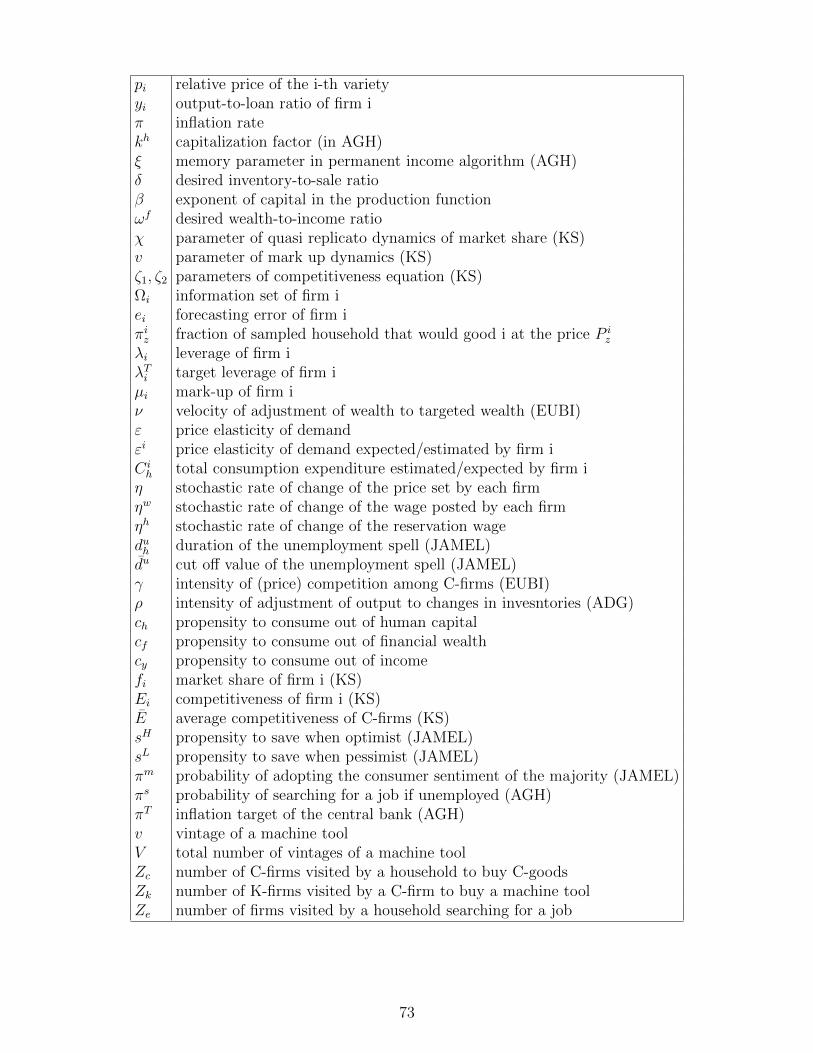
pi relative price of the i-th varietyyi output-to-loan ratio of firm iπ inflation ratekh capitalization factor (in AGH)ξ memory parameter in permanent income algorithm (AGH)δ desired inventory-to-sale ratioβ exponent of capital in the production functionωf desired wealth-to-income ratioχ parameter of quasi replicato dynamics of market share (KS)v parameter of mark up dynamics (KS)ζ1, ζ2 parameters of competitiveness equation (KS)Ωi information set of firm iei forecasting error of firm iπiz fraction of sampled household that would good i at the price P i

z

λi leverage of firm iλTi target leverage of firm iµi mark-up of firm iν velocity of adjustment of wealth to targeted wealth (EUBI)ε price elasticity of demandεi price elasticity of demand expected/estimated by firm iCih total consumption expenditure estimated/expected by firm i

η stochastic rate of change of the price set by each firmηw stochastic rate of change of the wage posted by each firmηh stochastic rate of change of the reservation wageduh duration of the unemployment spell (JAMEL)du cut off value of the unemployment spell (JAMEL)γ intensity of (price) competition among C-firms (EUBI)ρ intensity of adjustment of output to changes in invesntories (ADG)ch propensity to consume out of human capitalcf propensity to consume out of financial wealthcy propensity to consume out of incomefi market share of firm i (KS)Ei competitiveness of firm i (KS)E average competitiveness of C-firms (KS)sH propensity to save when optimist (JAMEL)sL propensity to save when pessimist (JAMEL)πm probability of adopting the consumer sentiment of the majority (JAMEL)πs probability of searching for a job if unemployed (AGH)πT inflation target of the central bank (AGH)v vintage of a machine toolV total number of vintages of a machine toolZc number of C-firms visited by a household to buy C-goodsZk number of K-firms visited by a C-firm to buy a machine toolZe number of firms visited by a household searching for a job

73

References

Anufriev, M., Assenza, T., Hommes, C. & Massaro, D. (2013), ‘Interest rules and macroeco-nomic stability under hetergenous expectations’, Macroeconomic Dynamics 17, 1574–1604.

Arifovic, J. (1995), ‘Genetic algorithms and inflationary economies’, Journal of MonetaryEconomics 36, 219–243.

Arifovic, J. (1996), ‘The behavior of the exchange rate in the genetic algorithm and experi-mental economies’, Journal of Political Economy 104, 510–541.

Arifovic, J., Bullard, J. & Kostyshyna, O. (2013), ‘Social learning and monetary policy rules’,Economic Journal 123, 38–76.

Artinger, F. & Gigerenzer, G. (2016), Heuristic pricing in an uncertain market: Ecologicaland constructivist rationality, Working Paper.

Ashraf, Q., Gershman, B. & Howitt, P. (2016), ‘How inflation affects macroeconomic perfor-mance: An agent-based computational investigation’, Macroeconomic Dynamics 20, 558–581.

Ashraf, Q., Gershman, B. & Howitt, P. (2017), ‘Banks, market organization, and macroe-conomic performance: An agent-based computational analysis’, Journal of Economic Be-havior and Organization 135, 143–180.

Assenza, T., Delli Gatti, D. & Grazzini, J. (2015a), ‘Emergent dynamics of a macroeconomicagent based model with capital and credit’, Journal of Economic Dynamics and Control50, 5–28.

Assenza, T. & Gatti, D. D. (2013), ‘E pluribus unum: Macroeconomic modelling for multi-agent economies’, Journal of Economic Dynamics and Control 37, 1659–1682.

Assenza, T. & Gatti, D. D. (2017), ‘The financial transmissiom of shocks in a simple hybridmacroeconomic agent based model’, forthcoming in Journal of Evolutionary Economics .

Assenza, T., Grazzini, J., Hommes, C. & Massaro, D. (2015b), ‘Pq strategies in monopolisticcompetition: Some insights from the lab’, Journal of Economic Dynamics and Control50, 62–77.

Balint, T., Lamperti, F., Mandel, A., Napoletano, M., Roventini, A. & Sapio, A. (2017),‘Complexity and the economics of climate change: a survey and a look forward’, EcologicalEconomics 158, 252–265.

Barde, S. (2017), ‘A practical, accurate, information criterion for nth order markov pro-cesses’, Computational Economics 50, 281–324.

Bargigli, L., Riccetti, L., Russo, A. & Gallegati, M. (2014), ‘Network analysis and calibrationof the leveraged network-based financial accelerator’, Journal of Economic Behavior andOrganization 99(C), 109–125.

74

Battiston, S., Delli Gatti, D., Gallegati, M., Greenwald, B. & Stiglitz, J. (2007), ‘Creditchains and bankruptcy propagation in production networks’, Journal of Economic Dy-namics and Control 31, 2061–2084.

Benes, J., Kumhof, M. & Laxton, D. (2014), Financial crises in dsge models: A prototypemodel, IMF Working Paper 14/57, International Monetary Fund.

Bennett, R. & Bergmann, B. (1986), A microsimulated model of the United States Economy,The John Hopkins University Press, Baltimore.

Bergman, B. (1974), ‘A microsimulation of the macroeconomy with explicitly representedmoney flows’, Annals of Economic and Social Measurement 3, 475–489.

Bernanke, B. & Gertler, M. (1989), ‘Agency costs, net worth, and business fluctuations’,American Economic Review 79, 14–31.

Bernanke, B. & Gertler, M. (1990), ‘Financial fragility and economic performance’, QuarterlyJournal of Economics 105, 87–114.

Bernanke, B., Gertler, M. & Gilchrist, S. (1999), The financial accelerator in a quantitativebusiness cycle framework, in J. Taylor & M. Woodford, eds, ‘Handbook of Macroeco-nomics, Volume 1’, Amsterdam: North-Holland, pp. 1341–1393.

Breitmoser, Y. (2016), ‘The axiomatic foundation of logit’, MPRA Paper No. 74334 .

Caiani, A., Godin, A., Caverzasi, E., Gallegati, M., Kinsella, S. & Stiglitz, J. E. (2016a),‘Agent based-stock flow consistent macroeconomics: Towards a benchmark model’, Jour-nal of Economic Dynamics and Control 69, 375–408.

Caiani, A., Russo, A. & Gallegati, M. (2016b), Does inequality hamper inno-vation and growth? An AB-SFC analysis, Working paper available at ssrn:http://papers.ssrn.com/sol3/papers.cfm?abstract id=2790911.

Carroll, C. (1992), How does future income affect current consumption?, Working paper 126,board of governors of the federal reserve system.

Carroll, C. (1997), ‘Buffer-stock saving and the life cycle/permanent income hypothesis’,Quarterly Journal of Economics 112(1), 1–55.

Carroll, C. (2003), ‘Macroeconomic expectations of households and professional forecasters’,Quarterly Journal of Economics 118, 269–298.

Carroll, C. (2009), ‘Precautionary saving and the marginal propensity to consume out ofpermanent income’, Journal of Monetary Economics 56(6), 780–790.

Carroll, C. & Summers, L. (1991), Consumption growth parallels income growth: Some newevidence, in B. Bernheim & J. Shoven, eds, ‘National Saving and Economic Performance’,Chicago: University of Chicago Press, pp. 305–348.

Catullo, E., Gallegati, M. & Palestrini, A. (2015), ‘Towards a credit network based earlywarning indicator for crises’, Journal of Economic Dynamics and Control 50, 78–97.

75

Chiarella, C. & Di Guilmi, C. (2017), ‘Monetary policy and debt deflation: Some computa-tional experiments’, Macroeconomic Dynamics 21, 214–242.

Cincotti, S., Raberto, M. & Teglio, A. (2010), ‘Credit money and macroeconomic instabilityin the agent-based model and simulator eurace’, Economics: The Open-Access, Open-Assessment E-Journal 4, 1–32.

Cincotti, S., Raberto, M. & Teglio, A. (2012a), The eurace macroeconomic model and simu-lator, in M. Aoki, K. Binmore, S. Deakin & H. Gintis, eds, ‘Complexity and Institutions:Markets, Norms and Corporations’, New York: Palgrave Macmillan, pp. 81–106.

Cincotti, S., Raberto, M. & Teglio, A. (2012b), ‘Macroprudential policies in an agent-basedartificial economy’, Revue de l’OFCE 124, 205–234.

Cioppa, T. & Lucas, T. (2007), ‘Efficient nearly orthogonal and space-filling latin hyper-cubes’, Technometrics pp. 45–55.

Colander, D., Howitt, P., Kirman, A., Leijonhufvud, A. & Mehrling, P. (2008), ‘Beyond dsgemodels: Toward an empirically based macroeconomics’, The American Economic Review:Papers and Proceedings 98, 236–240.

Dawid, H. & Gemkow, S. (2014), ‘How do social networks contribute to wage inequality?insights from an agent-based analysis’, Industrial and Corporate Change 23, 1171–1200.

Dawid, H., Gemkow, S., Harting, P. & Neugart, M. (2009), ‘On the effects of skill upgradingin the presence of spatial labor market frictions: an agent-based analysis of spatial policydesign’, Journal of Artifical Societies and Social Simulation – JASSS 12, 4.

Dawid, H., Gemkow, S., Harting, P. & Neugart, M. (2012), ‘Labor market integration policiesand the convergence of regions: the role of skills and technology diffusion’, Journal ofEvolutionary Economics 22, 543–562.

Dawid, H., Gemkow, S., Harting, P., Neugart, M., Kabus, K. & Wersching, K. (2008),‘Skills, innovation and growth: an agent-based policy analysis’, Journal of Economics andStatistics 228, 251–275.

Dawid, H., Gemkow, S., Harting, P., van der Hoog, S. & Neugart, M. (2018a), Agent-basedmacroeconomic modeling and policy analysis: The eurace@unibi model, in S.-H. Chen& M. Kaboudan, eds, ‘Handbook on Computational Economics and Finance’, OxfordUniversity Press.

Dawid, H. & Harting, P. (2012), Capturing firm behavior in agent-based models of industryevolution and macroeconomic dynamics, in G. Bunsdorf, ed., ‘Evolution, Organizationand Economic Behavior’, Edward Elgar, chapter 6.

Dawid, H., Harting, P. & Neugart, M. (2013), ‘Cohesion policy and inequality dynamics:Insights from a heterogeneous agents macroeconomic model’, Bielefeld Working Papers inEconomics and Management No. 26/2013 .

Dawid, H., Harting, P. & Neugart, M. (2014), ‘Economic convergence: Policy implicationsfrom a heterogeneous agent model’, Journal of Economic Dynamics and Control 44, 54–80.

76

Dawid, H., Harting, P. & Neugart, M. (2018b), ‘Fiscal transfers and regional economicgrowth’, forthcoming in Review of International Economics .

Dawid, H., Harting, P., van der Hoog, S. & Neugart, M. (2018c), ‘A heterogeneous agentmacroeconomic model for policy evaluation: Improving transparency and reproducibility’,forthcoming in Journal of Evolutionary Economics .

Deaton, A. (1991), ‘Saving and liquidity constraints’, Econometrica 59, 1221–1248.

Deissenberg, C., van der Hoog, S. & Dawid, H. (2008), ‘Eurace: A massively parallel agent-based model of the european economy’, Applied Mathematics and Computation 204, 541–552.

Delli Gatti, D. & Desiderio, S. (2015), ‘Monetary policy experiments in an agent-based modelwith financial frictions’, Journal of Economic Interaction and Coordination 10, 265–286.

Delli Gatti, D., Di Guilmi, C., Gaffeo, E., Giulioni, G., Gallegati, M. & Palestrini, A. (2005),‘A new approach to business fluctuations: heterogeneous interacting agents, scaling lawsand financial fragility’, Journal of Economic Behavior and Organization 56, 489–512.

Delli Gatti, D., Gallegati, M., Cirillo, P., Desiderio, S. & Gaffeo, E. (2011), Macroeconomicsfrom the Bottom-up, Springer-Verlag, Berlin.

Delli Gatti, D., Gallegati, M., Greenwald, B., Russo, A. & Stiglitz, J. (2010), ‘The financialaccelerator in an evolving credit network’, Journal of Economic Dynamics and Control34, 1627–1650.

Delli Gatti, D., Gallegati, M., Greenwald, B., Russo, A. & Stiglitz, J. E. (2006), ‘Busi-ness fluctuations in a credit-network economy’, Physica A: Statistical Mechanics and itsApplications 370(1), 68–74.

Delli Gatti, D., Gallegati, M., Greenwald, B., Russo, A. & Stiglitz, J. E. (2009), ‘Busi-ness fluctuations and bankruptcy avalanches in an evolving network economy’, Journal ofEconomic Interaction and Coordination 4(2), 195–212.

Dosi, G., Fagiolo, G., Napoletano, M. & Roventini, A. (2013), ‘Income distribution, creditand fiscal policies in an agent-based Keynesian model’, Journal of Economic Dynamicsand Control 37, 1598–1625.

Dosi, G., Fagiolo, G., Napoletano, M., Roventini, A. & Treibich, T. (2015), ‘Fiscal andmonetary policies in complex evolving economies’, Journal of Economic Dynamics andControl 52, 166–189.

Dosi, G., Fagiolo, G. & Roventini, A. (2006), ‘An evolutionary model of endogenous businesscycles’, Computational Economics 27, 3–34.

Dosi, G., Fagiolo, G. & Roventini, A. (2008), ‘The microfoundations of business cycles: anevolutionary multi-agent model’, Journal of Evolutionary Economics 18, 413–432.

Dosi, G., Fagiolo, G. & Roventini, A. (2010), ‘Schumpeter meeting Keynes: a policy-friendlymodel of endogenous growth and business cycles’, Journal of Economic Dynamics andControl 34, 1748–1767.

77

Dosi, G., Napoletano, M., Roventini, A. & Treibich, T. (2017a), ‘Micro and macro policiesin the Keynes plus Schumpeter evolutionary models’, Journal of Evolutionary Economics27, 63–90.

Dosi, G., Pereira, M., Roventini, A. & Virgillito, M. (2018), The effects of labour marketreforms upon unemployment and income inequalities: an agent based model approach,forthcoming in Socio-Economic Review.

Dosi, G., Pereira, M., Roventini, A. & Virgillito, M. (2017b), Causes and consequences ofhysteresis: Aggregate demand, productivity and employment, LEM Working Paper No.2017/07.

Dosi, G., Roventini, A. & Russo, E. (2017c), Endogenous growth and global divergence in amulti-country agent-based model, LEM Working Paper No. 2017/32.

Dosi, G., Pereira, M., Roventini, A. & Virgillito, M. (2017d), ‘When more flexibility yieldsmore fragility: the microfoundations of Keynesian aggregate unemployment’, Journal ofEconomic Dynamics and Control 81, 162–186.

Eliason, G. (1977), ‘Competition and market processes in a simulation model of the swedisheconomy’, American Economic Review 67, 277–281.

Eliason, G. (1984), ‘Micro-heterogeneity of firms and the stability of industrial growth’,Journal of Economic Behavior and Organization 5, 249–274.

Erlingsson, E. J., Raberto, M., Stefnsson, H. & Sturluson, J. T. (2013), Integrating the hous-ing market into an agent-based economic model, in A. Teglio, S. Alfarano, E. Camacho-Cuena & M. Gins-Vilar, eds, ‘Managing market complexity’, Lecture Notes in Economicsand Mathematical Systems, Springer.

Erlingsson, E., Teglio, A., Cincotti, S., Stefansson, H., Sturluson, J. T. & Raberto, M.(2014), ‘Housing market bubbles and business cycles in an agent-based credit economy’,ECONOMICS: THE OPEN-ACCESS, OPEN-ASSESSMENT E-JOURNAL 8.

Fagiolo, G. & Roventini, A. (2011), ‘On the scientific status of economic policy: A tale ofalternative paradigms’, forthcoming in the Knowledge Engineering Review .

Fagiolo, G. & Roventini, A. (2017), ‘Macroeconomic policy in dsge and agent-based modelsredux: New developments and challenges ahead’, Journal of Artificial Societies and SocialSimulation 20, 1.

Fontana, M. (2010), ‘The santa fe perspective on economics: Emerging patterns in the scienceof complexity’, History of Economic Ideas 18, 167–196.

Gaffeo, E., Catalano, M., Clementi, F., Delli Gatti, D., Gallegati, M. & Russo, A. (2007),‘Reflections on modern macroeconomics: Can we travel along a safer road?’, Physica A:Statistical Mechanics and its Applications 382(1), 68–74.

Gaffeo, E., Gallegati, M. & Gostoli, U. (2015), ‘An agent-based ”proof of principle” forwalrasian macroeconomic theory’, Computational and Mathematical Organization Theory21), 150–183.

78

Gali, J. (2008), Monetary policy,inflation and the business cycle, Princeton University Press,Princeton, New Jersey.

Gigerenzer, G. & Gaissmaier, W. (2011), ‘Heuristic decision making’, Annual Review ofPsychology 62, 451–482.

Goudet, O., Kant, J.-D. & Ballot, G. (2015), Forbidding fixed duration contracts: Unfoldingthe opposing effects with a multiagent model of the french labour market, in F. Amblard,F. Miguel, A. Blanchet & B. Gaudou, eds, ‘Advances in Artificial Economics, LectureNotes in Economics and Mathematical Systems, Vol. 676’, Springer: Berlin, pp. 151–167.

Grazzini, J., M.G.Richiardi & Tsionas, M. (2017), ‘Bayesian estimation of agent-based mod-els’, Journal of Economic Dynamics and Control 77, 26–47.

Greenwald, B. & Stiglitz, J. (1993), ‘Financial markets imperfections and business cycles’,Quarterly Journal of Economics 108, 77–113.

Gualdi, S., Tarzia, M., Zamponi, F. & Bouchaud, J. (2015), ‘Tipping points in macroeco-nomic agent-based models’, Journal of Economic Dynamics and Control 50(1), 29–61.

Guerini, M. & Moneta, A. (2017), ‘A method for agent-based models validation’, Journal ofEconomic Dynamics and Control 82, 125–141.

Haas, A. & Jaeger, C. (2005), ‘Agents, bayes, and climate risks - a modular modellingapproach’, Advances in Geosciences 4, 3–7.

Haber, G. (2008), ‘Monetary and fiscal policy analysis with an agent-based macroeconomicmodel’, Journal of Economics and Statistics 228, 276–205.

Haldane, A. (2016), The dappled world, http://www.bankofengland.co.uk/publications/pages/speeches/2016/937.aspx.

Harting, P. (2015), ‘Stabilization policies and long term growth: Policy implications froman agent-based macroeconomic model’, Bielefeld Working Papers in Economics and Man-agement No. 06-2015 .

Haruvy, E., Roth, A. & Unver, U. (2006), ‘The dynamics of law clerk matching: An experi-mental and computational investigation of proposals for reform of the market’, Journal ofEconomic Dynamics and Control 30, 457–486.

Holcombe, M., Coakley, S., Kiran, M., Chin, S., Greenough, C., Worth, D., Cincotti, S.,Raberto, M., Teglio, A., Deissenberg, C., van der Hoog, S., Dawid, H., Gemkow, S.,Harting, P. & Neugart, M. (2013), ‘Large-scale modeling of economic systems’, ComplexSystems 22, 175–191.

Hommes, C. (2013), Behavioral Rationality and Heterogeneous Expectations in Complex Eco-nomic Systems, Cambridge University Press.

Hommes, C., Sonnemans, J., Tuinstra, J. & van de Velden, H. (2005), ‘Coordination ofexpectations in asset pricing experiments’, Review of Financial Studies 18, 955–980.

79

Howitt, P. (2012), ‘What have central bankers learned from modern macroeconomic theory?’,Journal of Macroeconomics 34, 11–22.

Kirman, A. (1992), ‘Whom or what does the representative individual represent?’, Journalof Economic Perspectives 6, 117–136.

Kirman, A. (2016), ‘Ants and nonoptimal self-organization: Lessons for macroeconomics’,Macroeconomic Dynamics 20, 601–621.

Kiyotaki, N. & Moore, J. (1997), ‘Credit cycles’, Journal of Political Economy 105, 211–248.

Klimek, P., Poledna, S., Farmer, J. & Thurner, S. (2015), ‘To bail-out or to bail-in? answersfrom an agent-based model’, Journal of Economic Dynamics and Control 50, 144–154.

Krug, S. (2015), The interaction between monetary and macroprudential policy: Should cen-tral banks ”lean against the wind” to foster macrofinancial stability?, Economics WorkingPaper, Christian-Albrechts-Universitt Kiel, Department of Economics, No. 2015-08.

Krug, S. & Wohltmann, H.-W. (2016), ‘Shadow banking, financial regulation and animal spir-its: An ace approach’, Economics Working Paper, Christian-Albrechts-Universitat Kiel,Department of Economics, No. 2016-08 .

Lamperti, F., Dosi, G., Napoletano, M., Roventini, A. & Sapio, A. (2017), Faraway, so close:Coupled climate and economic dynamics in an agent-based integrated assessment model,LEM Working Paper 2017/12.

Lengnick, M. (2013), ‘Agent-based macroeconomics: A baseline model’, Journal of EconomicBehavior and Organization 86, 102–120.

Lengnick, M. & Wohltmann, H.-W. (2011), Agent-based financial markets and new keynesianmacroeconomics: A synthesis, Economics working paper, christian-albrechts-universitatkiel, department of economics, no. 2011,09.

Lengnick, M. & Wohltmann, H.-W. (2016), ‘Optimal monetary policy in a new keynesianmodel with animal spirits and financial markets’, Journal of Economic Dynamics andControl 64, 148–165.

Mandel, A., Jaeger, C., Fuerst, S., Lass, W., Lincke, D., Meissner, F., Pablo-Marti, F.& Wolf, S. (2010), ‘Agent-based dynamics in disaggregated growth models’, Centre dE-conomie de la Sorbonne Working Paper 10077 .

Minsky, H. (1963), Can ”it” happen again, in D. Carson, ed., ‘Banking and MonetaryStudies’, Richard D. Irwin: Homewood.

Napoletano, M., Dosi, G., Fagiolo, G. & Roventini, A. (2012), ‘Wage formation, investmentbehavior and growth regimes: an agent-based analysis’, Revue de l’OFCE 124, 235–261.

Napoletano, M., Roventini, A. & Gaffard, J.-L. (2015), Time-varying fiscal multipliers in anagent-based model with credit rationing, GREDEG Working Paper No. 2015-30.

80

Neugart, M. & Richiardi, M. (2018), Agent-based models of the labor market, in S.-H. Chen& M. Kaboudan, eds, ‘Handbook on Computational Economics and Finance’, OxfordUniversity Press.

Neveu, A. (2013), ‘Fiscal policy and business cycle characteristics in a heterogeneous agentmacro model’, Journal of Economic Behavior and Organization 90, 224–240.

Ozel, B., Nathanael, R., Raberto, M., Teglio, A. & Cincotti, S. (2016), Macroeconomicimplications of mortgage loans requirements: An agent based approach, Working Papers2016/05, Economics Department, Universitat Jaume I, Castelln.

Petrovic, M., Ozel, B., Teglio, A., Raberto, M. & Cincotti, S. (2017), Eurace open: Anagent-based multi-country model, Universtiy Jaume I Working Papers No. 2017/09.

Piva, M. & Vivarelli, M. (2009), ‘Corporate skills as an ex-ante incentive to R&D investment’,International Journal of Manpower 30, 835–852.

Ponta, L., Raberto, M. & Cincotti, S. (2018), ‘An agent-based stock-flow consistent modelof the sustainable transition in the energy sector’, Ecological Economics 145, 274–300.

Popoyan, L., Napoletano, M. & Roventini, A. (2017), ‘Taming macroeconomic instability:Monetary and macro-prudential policy interactions in an agent-based model’, Journal ofEconomic Behavior and Organization 134, 117–140.

Raberto, M., Cincotti, S. & Teglio, A. (2014), Fiscal consolidation and sovereign debt riskin balance-sheet recessions: an agent-based approach, in P. T. L. Manica, ed., ‘EconomicPolicy and the Financial Crisis’, Routledge.

Raberto, M., Nathanael, R., Ozel, B., Teglio, A. & Cincotti, S. (2017), Credit-driven businesscycles in an agent-base macro model, in M. S.-W. H. Hanappi, S.s Katsikides, ed., ‘Theoryand method of evolutionary political economy’, Routledge.

Raberto, M., Ozel, B., Ponta, L., Teglio, A. & Cincotti, S. (2018), ‘From financial insta-bility to green finance: the role of banking and monetary policies in the eurace model’,forthcoming in Journal of Evolutionary Economics .

Raberto, M., Teglio, A. & Cincotti, S. (2008), ‘Integrating real and financial markets in anagent-based economic model: an application to monetary policy design’, ComputationalEconomics 32, 147–162.

Raberto, M., Teglio, A. & Cincotti, S. (2012), ‘Debt, deleveraging and business cycles:an agent-based perspective’, Economics, The Open-Access, Open-Assessment E-Journal6(2012-27).

Riccetti, L., Russo, A. & Gallegati, M. (2013), ‘Leveraged network-based financial accelera-tor’, Journal of Economic Dynamics and Control 37(8), 1626–1640.

Riccetti, L., Russo, A. & Gallegati, M. (2015), ‘An agent based decentralized match-ing macroeconomic model’, Journal of Economic Interaction and Coordination vol.10(2), 305–332.

81

Riccetti, L., Russo, A. & Gallegati, M. (2016a), ‘Financialisation and crisis in an agent basedmacroeconomic model’, Economic Modelling 52(PA), 162–172.

Riccetti, L., Russo, A. & Gallegati, M. (2016b), ‘Stock market dynamics, leveraged network-based financial accelerator and monetary policy’, International Review of Economics andFinance 43(C), 509–524.

Riccetti, L., Russo, A. & Gallegati, M. (2017), ‘Financial regulation and endogenous macroe-conomic crises’, forthcoming in Macroeconomic Dynamics .

Riccetti, L., Russo, A. & Gallegati, M. (2018), ‘Financial regulation and endogenous macroe-conomic crises’, forthcoming in Macroeconomic Dynamics .

Richiardi, M. (2017), ‘The future of agent-based modeling’, Eastern Economic Journal43, 271–287.

Romer, P. (2016), The trouble with macroeconomics, forthcoming in The AmericanEconomist.

Russo, A., Catalano, M., Gaffeo, E., Gallegati, M. & Napoletano, M. (2007), ‘Industrialdynamics, fiscal policy and r&d: Evidence from a computational experiment’, Journal ofEconomic Behavior and Organization 64, 426–447.

Russo, A., Riccetti, L. & Gallegati (2016), ‘Increasing inequality, consumer credit and finan-cial fragility in an agent based macroeconomic model’, Journal of Evolutionary Economics26, 25–47.

Salle, I. (2015), ‘Modeling expectations in agent-basedmodelsan application to central bank’scommunication and monetary policy’, Economic Modelling 46, 130–141.

Salle, I., Yldzoglu, M. & Senegas, M.-A. (2013), ‘Inflation targeting in a learning economy:An abm perspective’, Economic Modelling 34, 114–128.

Seppecher, P. (2012), ‘Flexibility of wages and macroeconomic instability in an agent-basedcompuational model with endogenous money’, Macroeconomic Dynamics 16, 284–297.

Seppecher, P. & Salle, I. (2015), ‘Deleveraging crises and deep recessions: a behaviouralapproach’, Applied Economics 47, 3771–3790.

Seppecher, P., Salle, I. & Lavoie, M. (2018), ‘What drives markups? evolutionary pricingin an agent-based stock-flow consistent macroeconomic model’, forthcoming in Industrialand Corporate Change .

Simon, H. (1959), ‘Theories of decision-making in economics and behavioral science’, Amer-ican Economic Review 49, 253–283.

Sims, C. (1980), ‘Macroeconomics and reality’, Econometrica 48, 1–48.

Sinitskaya, E. & Tesfatsion, L. (2015), ‘Macroeconomies asconstructivelyrationalgames’,Journal of Economic Dynamics and Control 61, 152–182.

82

Teglio, A., Cincotti, S., Erlingsson, E., Raberto, M., Stefansson, H. & Sturluson, J. (2014),Subprime lending and financial inequality in an agent-based model, in S. Leitner & F. Wall,eds, ‘Artificial Economics and Self Organization’, Lecture Notes in Economics and Math-ematical Systems, Springer.

Teglio, A., Mazzocchetti, A., Ponta, L., Raberto, M. & Cincotti, S. (2018), ‘Budgetary rigourwith stimulus in lean times: Policy advices from an agent-based model’, forthcoming inJournal of Economic Behavior and Organization .

Teglio, A., Raberto, M. & Cincotti, S. (2010), Endogenous credit dynamics as source of busi-ness cycles in the eurace model, in M. L. Calzi, L. Milone & P. Pellizzari, eds, ‘Progressin Artificial Economics. Computational and Agent-Based Models’, Lecture Notes in Eco-nomics and Mathematical Systems, Springer.

Teglio, A., Raberto, M. & Cincotti, S. (2012), ‘The impact of banks capital adequacy regu-lation on the economic system: an agent-based approach’, Advances in Complex Systems15.

Tesfatsion, L. (2006), Agent-based computational economics: A constructive approach toeconomic theory, in L. Tesfatsion & K. Judd, eds, ‘Handbook of Computational Economics,Volume II’, North-Holland, pp. 831–880.

Tesfatsion, L. & Judd, K. E. (2006), Handbook of Computational Economics II: Agent-BasedComputational Economics, North-Holland.

Trichet, J. (2010), Reflections on the nature of monetary policy non-standard measures andfinance theory, http://www.ecb.europa.eu/press/key/date/2010/html/sp101118.en.html.

van der Hoog, S. (2018), ‘The limits to credit growth: Mitigation policies and macropru-dential regulations to foster macrofinancial stability and sustainable debt’, forthcoming inComputational Economics .

van der Hoog, S. & Dawid, H. (2017), ‘Bubbles, crashes and the financial cycle: Insights froma stock-flow consistent agent-based macroeconomic model’, forthcoming in MacroeconomicDynamics .

Wolf, S., Furst, S., Mandel, A., Lass, W., Lincke, D., Pablo-Martı, F. & Jaeger, C. (2013),‘A multi-agent model of several economic regions’, Environmental Modelling & Software44, 25–43.

83