DOES THE CHOICE OF PERFORMANCE MEASURE INFLUENCE THE

EVALUATION OF HEDGE FUNDS?

MARTIN ELING

FRANK SCHUHMACHER

WORKING PAPERS ON RISK MANAGEMENT AND INSURANCE NO. 29

EDITED BY HATO SCHMEISER

CHAIR FOR RISK MANAGEMENT AND INSURANCE

SEPTEMBER 2006

1

DOES THE CHOICE OF PERFORMANCE MEASURE INFLUENCE THE EVALUATION

OF HEDGE FUNDS?

Martin Eling

Frank Schuhmacher∗∗∗∗

JEL classification: D81; G10; G11; G29

ABSTRACT

The Sharpe ratio is adequate for evaluating investment funds when the returns of those funds are normally distributed and the investor intends to place all his risky as-sets into just one investment fund. Hedge fund returns differ significantly from a normal distribution. For this reason, other performance measures for hedge fund re-turns have been proposed in both the academic and practice-oriented literature. In conducting an empirical study based on return data of 2,763 hedge funds, we com-pare the Sharpe ratio with 12 other performance measures. Despite significant devia-tions of hedge fund returns from a normal distribution, our comparison of the Sharpe ratio to the other performance measures results in virtually identical rank ordering across hedge funds.

1. Introduction

Financial analysts and, often, individual investors themselves rely heavily on risk-adjusted re-

turn (i.e., “performance”) measures to select among available investment funds. The most

widely known performance measure is the Sharpe ratio, which measures the relationship be-

tween the risk premium and the standard deviation of the returns generated by a fund (see

Sharpe, 1966). The Sharpe ratio is an adequate performance measure if the returns of the

funds are normally distributed1 and the investor wishes to place all his risky assets in just one

fund.2 However, there are many other performance measures and there are two good argu-

ments for the application of performance measures other than the Sharpe ratio.

∗ Martin Eling is with the Institute of Insurance Economics, University of St. Gallen, Kirchlistrasse 2, 9010 St.

Gallen, Switzerland, Tel.: +41 71 243 40 93, Fax: +41 71 243 40 40, E-Mail: martin.eling@unisg.ch. Frank

Schuhmacher is with the Department of Finance, University of Leipzig, Jahnallee 59, 04109 Leipzig, Ger-

many, Tel.: +49 341 973 36 70, Fax: +49 341 973 36 79, E-Mail: schuhmacher@wifa.uni-leipzig.de

1 More generally, if the asset returns obey an elliptical distribution, mean-variance analysis is consistent with

expected-utility analysis. See Chamberlain (1983). The normal distribution is an example of an elliptical dis-

tribution. If the investor’s utility function can be approximated by a quadratic utility function, mean-variance

analysis is also consistent with expected utility analysis.

2 For a justification of the Sharpe ratio from an analysis of an investor’s portfolio selection problem, see Bodie,

Kane, and Marcus (2005, p. 871).

2

First, a performance measure adequate for an investor who invests all his risky assets in just

one fund may not be appropriate for an investor who splits the risky assets, e.g., between a

market index and an investment fund (see, e.g., Bodie, Kane, and Marcus, 2005). The Sharpe

ratio is appropriate in the first case, while in the second case, a performance measure that also

takes into account the correlation between the market index and the respective fund would be

more suitable.3 Such measures include the Treynor and Jensen measures (see Treynor, 1965;

Jensen, 1968).4

The second argument (put forth by many authors) for using a performance measure other than

the Sharpe ratio is that the choice of an adequate performance measure depends on the fund’s

return distribution. In case of normally distributed returns, performance measures that rely on

the first two moments of the return distribution (expected value, standard deviation), as does

the Sharpe ratio, are appropriate. As hedge funds frequently generate returns that have a non-

normal distribution, it is commonly believed that these funds cannot be adequately evaluated

using the classic Sharpe ratio (see, e.g., Brooks and Kat, 2002; Mahdavi, 2004; Sharma,

2004). Consideration of this issue has led to the development of new performance measures,

which are currently under debate in hedge fund literature.

In the following we analyze and compare 13 different performance measures: the Sharpe’s,

Treynor’s, and Jensen’s measures, as well as Omega, the Sortino ratio, Kappa 3, the upside

potential ratio, the Calmar ratio, the Sterling ratio, the Burke ratio, the excess return on value

at risk, the conditional Sharpe ratio, and the modified Sharpe ratio. Using these measures, we

analyze 2,763 hedge funds to find an answer to the question of whether the ranking of the

funds depends in a critical way on the choice of the performance measure.

The motivation for the analysis comes from recent research in which the choice of a particular

measure has no significant influence on the ranking of an investment. Pfingsten, Wagner, and

Wolferink (2004) compared rank correlations for various risk measures on the basis of an in-

vestment bank’s 1999 trading book. In doing so, they found that different measures result in a

largely identical ranking. Pedersen and Rudholm-Alfvin (2003) compared risk-adjusted per-

formance measures for various asset classes over the period from 1998 to 2003. They found a

3 For the use of the Sharpe ratio in the second case, see Dowd (2000).

4 For a justification of these measures from an analysis of an investor’s portfolio selection problem, see

Breuer, Gürtler, and Schuhmacher (2004, pp. 379–396) or Scholz and Wilkens (2003).

3

high rank correlation between the performance measures’ rankings. In the hedge fund context,

Eling and Schuhmacher (2005) found a high rank correlation between different performance

measures using hedge fund indices data from 1994 to 2003.

This study builds on these earlier studies as follows. In contrast to Pedersen and Rudholm-

Alfvin (2003), we concentrate on hedge funds as an asset class, performance measures pro-

posed for hedge funds, and the related debate concerning the suitability of classic and newer

measures for the evaluation of hedge funds. In contrast to Eling and Schuhmacher (2005), we

analyze individual hedge fund data instead of indices. Furthermore, we analyze the situation

in which the fund under consideration represents the entire risky investment as well as the

situation in which the fund represents only a portion of the investor’s wealth.

The result of our analysis can be summarized as follows: Despite significant deviations of

hedge fund returns from a normal distribution, our comparison of the Sharpe ratio to other

measures results in virtually identical rank ordering across the hedge funds.

The remainder of the paper is organized as follows. In Section 2, the performance measures

are presented. Section 3 and 4 comprise an empirical study where all 13 measures are em-

ployed for determining the performance of 2,763 hedge funds. In Section 3 we consider the

decision-making situation where the fund under evaluation represents the entire risky invest-

ment. In Section 4 we examine the decision-making situation where the fund under evaluation

represents only a portion of the investor’s wealth. In both sections, the data and the methodol-

ogy are explained (Sections 3.1 and 4.1), the results of the performance measurement are pre-

sented (Sections 3.2 and 4.2), and robustness tests are conducted (Sections 3.3 and 4.3). The

results of the study are summarized in Section 5.

2. Classic and newer approaches to measuring performance

2.1. Classic performance measurement—The Sharpe ratio

In hedge fund analysis, the Sharpe ratio is frequently chosen as the performance measure and

a comparison is made with the Sharpe ratios of other funds or market indices (see, e.g.,

Ackermann, McEnally, and Ravenscraft, 1999; Liang, 1999; Schneeweis, Kazemi, and Mar-

tin, 2002). Using historical monthly returns ri1, …, riT for investment fund i, the Sharpe ratio

can be calculated as follows:

4

d

i fi

i

r rSharpe Ratio

σ

−= . (1)

rid = (ri1 + … + riT)/T represents the average monthly return for security i, rf the risk-free

monthly interest rate, and σi = (((ri1 – rid)2 + … + (riT – ri

d)2)/(T – 1))0.5 the standard deviation

of the monthly return. However, use of the Sharpe ratio in hedge fund performance measure-

ment is the subject of intense criticism because hedge fund returns do not display a normal

distribution (see Kao, 2002; Amin and Kat, 2003; Gregoriou and Gueyie, 2003). For example,

the use of derivative instruments results in an asymmetric return distribution, as well as fat

tails, leading to the danger that the use of standard risk and performance measures will under-

estimate risk and overestimate performance (see Kat, 2003; McFall Lamm, 2003; Geman and

Kharoubi, 2003). To avoid this problem, newer performance measures that illustrate the risk

of loss are recommended (see Pedersen and Rudholm-Alfvin, 2003; Lhabitant, 2004).

2.2. Newer approaches to performance measurement

2.2.1. Measuring performance on the basis of lower partial moments

Lower partial moments (LPMs) measure risk by negative deviations of the returns realized in

relation to a minimal acceptable return τ. The LPM of order n for security i is calculated as

( ) [ ]∑=

−=T

1t

n

itni ,0rτmaxT

1τLPM .

Because LPMs consider only negative deviations of returns from a minimal acceptable return

(which could be zero, the risk-free rate, or the average return), they seem to be a more appro-

priate measure of risk than the standard deviation, which considers negative and positive de-

viations from expected return (see Sortino and van der Meer, 1991). The choice of order n de-

termines the extent to which the deviation from the minimal acceptable return is weighted.

The LPM of order 0 can be interpreted as shortfall probability, LPM of order 1 as expected

shortfall, and LPM of order 2 for τ = rid as semi-variance. The LPM order chosen should be

higher the more risk averse an investor is. Omega (see Shadwick and Keating, 2002), the

Sortino ratio (see Sortino and van der Meer, 1991), and Kappa 3 (see Kaplan and Knowles,

2004) use LPMs of order 1, 2, or 3:5

5 Equation (2) is not identical to the definition originally suggested by Shadwick and Keating (2002) for

Omega, but is based on an equivalent representation that can be interpreted more easily than the original

definition. For a derivation of Equation (2), see Kaplan and Knowles (2004).

5

( )

d

ii

1i

r τOmega 1

LPM τ

−= + , (2)

( )

d

ii

22i

r τSortinoRatio

LPM τ

−= , (3)

( )

d

ii

33i

r τKappa 3

LPM τ

−= . (4)

Note that these measures compute the excess return as the difference between the average re-

turn and the minimal acceptable return. Another way of measuring excess return is to use a

higher partial moment (HPM), which measures positive deviations from the minimal accept-

able return τ. The upside potential ratio (see Sortino, van der Meer, and Plantinga, 1999)

combines the HPM of order 1 with the LPM of order 2. The advantage of this ratio is the con-

sistent application of the minimal acceptable return in the numerator as well as in the denomi-

nator:

( )

( )1i

i2

2i

HPM τUpside Potential Ratio

LPM τ= . (5)

2.2.2. Measuring performance on the basis of drawdown

Drawdown-based measures are particularly popular in practice. They often are used by com-

modity trading advisors because these measures illustrate what the advisors are supposed to

do best—continually accumulating gains while consistently limiting losses (see Lhabitant,

2004).

The drawdown of a security is the loss incurred over a certain investment period. In describ-

ing drawdown-based risk measures, rit-т denotes the return realized over the period from t to т

(t < т ≤ T). For all these returns, MDi1 denotes the lowest return and MDi2 the second lowest

return, and so on. In general, the smallest return, MDi1, is negative and denotes the maximum

possible loss that could have been realized in the considered period of time. The Calmar ra-

tio (see Young, 1991), Sterling ratio (see Kestner, 1996), and Burke ratio (see Burke, 1994)

use the maximum drawdown, an average above the N largest drawdowns (which does not re-

act too sensitively to outliers), and a type of variance above the N largest drawdowns (which

6

takes into account that a number of very large losses might represent a greater risk than sev-

eral small declines) as risk measures:6

d

i fi

i1

r rCalmar Ratio

MD

−=−

, (6)

d

i fi N

ij

j 1

r rSterling Ratio

1MD

N =

−=

−∑, (7)

d

i fi

N2

2ij

j 1

r rBurke Ratio

MD=

−=

∑. (8)

2.2.3. Measuring performance on the basis of value at risk

Value at risk has also been proposed as an alternative risk measure in hedge fund performance

measurement. Value at risk (VaRi) describes the possible loss of an investment, which is not

exceeded with a given probability of 1-α in a certain period. In case of normally distributed

returns, the so-called standard value at risk can be computed by VaRi = − (rid + zα⋅σi), where

zα denotes the α-quantile of the standard normal distribution. Instead of standard value at risk,

the literature frequently considers expected loss under the condition that the value at risk is

exceeded. This conditional value at risk is defined as CVaRi = E[− rit | rit ≤ −VaRi]. The ad-

vantage of conditional value at risk is that it satisfies certain plausible axioms (see Artzner et

al., 1999). If returns do not display a normal distribution pattern, the Cornish-Fisher expan-

sion can be used to include skewness and kurtosis in computing value at risk. The modified

value at risk based on the Cornish-Fisher expansion is calculated as: MVaRi = − (rid + σi⋅(zα +

(zα2–1)⋅Si/6 + (zα

3–3⋅zα)⋅Ei/24 – (2⋅zα3 – 5⋅zα)⋅Si

2/36)), where Si denotes skewness and Ei the

excess kurtosis for security i (see Favre and Galeano, 2002).

The performance measures excess return on value at risk (see Dowd, 2000), the conditional

Sharpe ratio (see Agarwal and Naik, 2004), and the modified Sharpe ratio (see Gregoriou

and Gueyie, 2003) can be used when risk is measured by standard value at risk, conditional

value at risk, or modified value at risk, respectively:

6 Defining the Calmar and the Sterling ratio, the maximum drawdown is preceded by a minus sign so that the

denominator is positive and higher values for the denominator represent a higher risk.

7

d

i fi

i

r rExcess Return on Value at Risk

VaR

−= , (9)

d

i fi

i

r rConditional Sharpe Ratio

CVaR

−= , (10)

d

i fi

i

r rModified Sharpe Ratio

MVaR

−= . (11)

2.3. Classic performance measurement—Jensen’s measure and Treynor’s ratio

There are two classic performance measures explicitly constructed for situations in which

only a small portion of the investor’s wealth is allocated to the hedge fund under considera-

tion.

The Jensen measure considers the average return of the fund above that predicted by the

capital asset pricing model. The beta factor (β) is generally calculated using the correlation

between the returns of a market index and the returns of the investment fund. However, for

the decision-making situation discussed in Section 4 (the hedge fund represents only a portion

of the investor’s wealth), it is appropriate to compute β by replacing the market index with a

so-called reference portfolio, which represents the investor’s portfolio without the hedge fund

(see Breuer, Gürtler, and Schuhmacher, 2004, pp. 374–396):

( ) ( )d d

i i f rp f iJensen Measure = r r r r β− − − ⋅ . (12)

The Jensen measure is often criticized because it can be manipulated by leveraging the fund

return. The Treynor ratio does not suffer from this defect. The Treynor ratio considers the

excess return of the fund in relation to its beta factor:

d

i fi

i

r rTreynor Ratio =

β

−. (13)

Again, as with Jensen’s measure, in our empirical analysis the beta factor is estimated on the

basis of the correlation between the hedge fund and the investor’s reference portfolio without

the hedge fund.

8

3. Measuring performance when the fund represents the entire risky investment

3.1. Data and methodology

We obtained hedge fund data from ehedge, a German financial services company founded in

2000 by the LCF Rothschild Group and bmp Venture Capital. The company provides hedge

fund information and other services to institutional investors (see www.ehedge.de). As of July

2005, the ehedge database contained 2,763 individual hedge funds reporting monthly net-of-

fee returns for the time period from 1985 to 2004.7 The database contains additional informa-

tion on each fund, such as company name, strategy description, assets under management, and

management fees. The database includes 2,106 (76.22%) surviving funds and 657 (23.78%)

dissolved funds. The total assets under management are about $229.47 billion, which is ap-

proximately one-quarter of the worldwide hedge fund market volume of $950 billion (for the

hedge fund market volume, see Van, 2005).8

The return distributions of the hedge funds are analyzed in Table 1. The table shows the

mean, the median, the standard deviation, the minimum, and the maximum of the first four

moments of the return distribution (mean value, standard deviation, skewness, and excess kur-

tosis). On basis of the Jarque-Bera test, the assumption of normally distributed hedge fund re-

turns must be rejected for 39.12% (44.08%) of the funds at the 1% (5%) significance level.

Table 1: Descriptive statistics for 2,763 hedge fund return distributions

Fund Mean Median Standard deviation Minimum Maximum

Mean value (%) 0.88 0.75 0.95 -4.87 15.72

Standard deviation (%) 3.18 2.14 3.12 0.06 32.79

Skewness 0.15 0.09 1.16 -8.91 8.55

Excess kurtosis 2.70 0.85 7.10 -7.34 89.07

7 For some hedge funds in the database there is also return data prior to 1985, but we choose to start our inves-

tigation in 1985 as there are too few observations before this point in time.

8 Like other hedge fund databases, the ehedge database suffers from some data biases. Survivorship bias is cal-

culated as the difference in fund returns between all funds and the surviving funds. In the ehedge database,

this difference amounts 0.06% per month, which is comparable to other values found in the literature. See,

e.g., Ackermann, McEnally, and Ravenscraft (1999) and Liang (2000). There also might be a backfilling

bias, as fund returns are in the database before its starting point in 2000. To take these bias problems into ac-

count, we conducted our investigation separately for surviving and for dissolved funds and for the time pe-

riod from 2000 to 2004 (see Section 3.3). However, none of these variations influence our main result.

9

The findings reported in the next section were generated by first using the measures presented

in Sections 2.1 and 2.2 to determine hedge fund performance. For the LPM-based perform-

ance measures we assume that the minimal acceptable return is equal to the risk-free monthly

interest rate (τ = 0.35%).9 For the Sterling and Burke ratios, the five largest drawdowns are

considered (N = 5). The value-at-risk-based performance measures were calculated using a

significance level of α = 0.05. Next, for each performance measure the funds were ranked on

the basis of the measured values. Finally, the rank correlations between the performance

measures were calculated.

3.2. Findings

In Table 2 we present the Spearman rank correlation coefficients between the performance

measures.10

Table 2: Rank correlation based on different performance measures

Performance measure

Sharpe ratio

Omega

Sortino ratio

Kappa 3

Upside potential

ratio

Calmar ratio

Sterling ratio

Burke ratio

Excess return on

value at risk

Conditional

Sharpe ratio

Modified

Sharpe ratio

Sharpe ratio

Omega 0.99

Sortino ratio 0.99 0.99

Kappa 3 0.98 0.98 1.00

Upside potential ratio 0.95 0.95 0.98 0.99

Calmar ratio 0.95 0.94 0.96 0.97 0.96

Sterling ratio 0.93 0.93 0.94 0.95 0.93 0.98

Burke ratio 0.95 0.94 0.96 0.97 0.95 0.99 0.99

Excess return on value at risk 1.00 0.98 0.98 0.97 0.94 0.95 0.94 0.95

Conditional Sharpe ratio 0.98 0.96 0.98 0.99 0.97 0.97 0.95 0.97 0.98

Modified Sharpe ratio 0.97 0.97 0.98 0.98 0.95 0.94 0.92 0.94 0.97 0.96

Average 0.97 0.96 0.98 0.98 0.96 0.96 0.95 0.96 0.97 0.97 0.96

All performance measures display a very high rank correlation with respect to the Sharpe ratio

as well as in relation to each other. The rank correlation coefficient for the Sharpe ratio varies

9 A constant risk-free interest rate of 0.35% per month was used. This corresponds to the interest rate on 10-

year U.S. Treasury bonds at 30 December 2004 (4.28% per annum). Alternatively, a rolling interest rate, an

average interest rate for the period under consideration, or the interest rate at the beginning of the investiga-

tion period could be used. All three approaches yield almost identical results.

10 In this and the following Table 5 we only display and calculate the bottom left triangle of the symmetric ma-

trix, not the values on the diagonal (1.00) or in the mirror image on the upper-right triangle of the matrix.

10

between 0.93 (Sterling ratio) and 1.00 (excess return on value at risk). On average, the rank

correlation of the Sharpe ratio in relation to the other performance measures amounts to 0.97.

There is also a very high correlation between the Sharpe ratio, Omega, the Sortino ratio, the

Sterling ratio, Kappa 3, and the conditional Sharpe ratio (rank correlation greater than 0.98 in

each case).

We also find high rank correlations when comparing the new performance measures to each

other. The highest possible rank correlation of 1.00 can be found when comparing Kappa 3

and the Sortino ratio, while the lowest value of 0.92 is found with the modified Sharpe ratio

and the Sterling ratio. The average rank correlation between the performance measures is

0.96.

We use two test statistics to check the significance of the rank correlations. First, statistical

significance is tested using a standardized version of the Hotelling-Pabst statistic. In this test,

the hypothesis of independence of the two related rankings is checked for all correlation coef-

ficients. However, even at the significance level of α = 0.01, there is no case in which the hy-

pothesis of independence can be confirmed. Therefore, the hypothesis of independence of the

measurement series must be rejected for all correlation coefficients.

Instead of testing whether the rankings are independent (in other words, the rank correlation is

zero), it is possible to check the hypothesis that the rank correlation is smaller than a certain

given rank correlation x. We did this using the Fisher transformation and found for a signifi-

cance level of α = 0.01 that the hypothesis that the rank correlation is smaller than x is re-

jected for all x smaller than 0.917 (see Rees, 1987, p. 383, for the test statistic).11

In conclusion, on the basis of our data, none of the new performance measures results in sig-

nificant changes in the evaluation of hedge funds as compared to that found using the Sharpe

ratio. Thus, it does not much matter which of the numerous measures is used to assess the per-

formance of hedge funds. Because the newer performance measures result in rankings that are

practically the same and thus each gives a similar assessments of hedge funds, use of the

11 Note that the second test is much stronger than the first test. Nevertheless, we report the results of the first

test because it is more widely known than the second test. We have not tested the hypothesis of unit correla-

tion because even for normally distributed returns we would not expect all correlations to be equal to 1.

11

Sharpe ratio (even if it displays some undesirable features) is justified, at least from a practi-

cal perspective.

3.3. Robustness of the findings

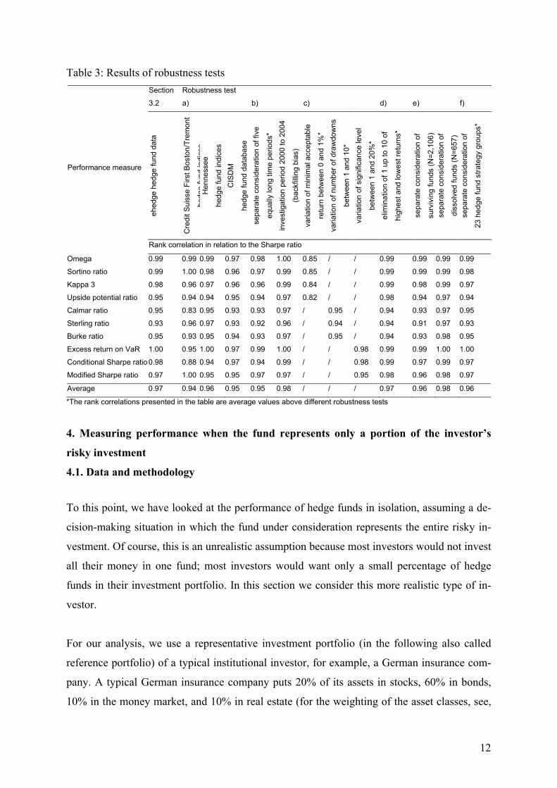
In Table 3 we report the results of various robustness tests. Instead of presenting the rank cor-

relation between all pairs of performance measures for each robustness test (as in Table 2), we

report only the (average) rank correlation between the Sharpe ratio and all other performance

measures. We found that the main result is robust with respect to:

a) variations of the database (in place of the ehedge database, we used the Credit Suisse First

Boston/Tremont hedge fund indices, the Hennessee hedge fund indices, and the Center for In-

ternational Securities and Derivatives Markets (CISDM) hedge fund database),

b) variations of the investigation period (we broke down the period from 1985 to 2004 into

five equally long time periods and we investigated separately the time period from 2000 to

2004 to account for the backfilling bias as explained in footnote 8),

c) variations of the exogenously fixed parameters (for the LPM-based measures, the minimal

acceptable return was varied between 0 and 1%, for the drawdown-based measures, the num-

ber of drawdowns was varied between 1 and 10, and for the VaR-based measures, the signifi-

cance level was varied between 0.01 and 0.20),

d) an elimination of outliers (we eliminated between 1 and 10 of the highest and lowest re-

turns from the time series),

e) a separate consideration of surviving funds and dissolved funds (to account for the survi-

vorship bias as explained in footnote 8), and

f) a separate consideration of 23 different hedge fund strategies.

For all these tests we find high rank correlations comparable to those presented in Section

3.2.12 Detailed results are available upon request.

12 The only noticeable deviation from the Sharpe ratio rankings can be found with the LPM-based measures if

the minimal acceptable return is higher than 0.50%. This is due to the way these performance measures are

constructed: as the minimum return increases, those strategies that display a high volatility of returns are fa-

vored because only those strategies have a sufficient number of returns that exceed the minimum return. This

results in changes in performance values and in considerable changes in rankings and rank correlation.

12

Table 3: Results of robustness tests

Robustness test Section

3.2 a) b) c) d) e) f)

ehedge hedge fund data

Credit Suisse First Boston/Tremont

hedge fund indices

Hennessee

hedge fund indices

CISDM

hedge fund database

separate consideration of five

equally long time periods*

investigation period 2000 to 2004

(backfilling bias)

variation of minimal acceptable

return between 0 and 1%*

variation of number of drawdowns

between 1 and 10*

variation of significance level

between 1 and 20%*

elim

ination of 1 up to 10 of

highest and lowest returns*

separate consideration of

surviving funds (N=2,106)

separate consideration of

dissolved funds (N=657)

separate consideration of

23 hedge fund strategy groups*

Performance measure

Rank correlation in relation to the Sharpe ratio

Omega 0.99 0.99 0.99 0.97 0.98 1.00 0.85 / / 0.99 0.99 0.99 0.99

Sortino ratio 0.99 1.00 0.98 0.96 0.97 0.99 0.85 / / 0.99 0.99 0.99 0.98

Kappa 3 0.98 0.96 0.97 0.96 0.96 0.99 0.84 / / 0.99 0.98 0.99 0.97

Upside potential ratio 0.95 0.94 0.94 0.95 0.94 0.97 0.82 / / 0.98 0.94 0.97 0.94

Calmar ratio 0.95 0.83 0.95 0.93 0.93 0.97 / 0.95 / 0.94 0.93 0.97 0.95

Sterling ratio 0.93 0.96 0.97 0.93 0.92 0.96 / 0.94 / 0.94 0.91 0.97 0.93

Burke ratio 0.95 0.93 0.95 0.94 0.93 0.97 / 0.95 / 0.94 0.93 0.98 0.95

Excess return on VaR 1.00 0.95 1.00 0.97 0.99 1.00 / / 0.98 0.99 0.99 1.00 1.00

Conditional Sharpe ratio 0.98 0.88 0.94 0.97 0.94 0.99 / / 0.98 0.99 0.97 0.99 0.97

Modified Sharpe ratio 0.97 1.00 0.95 0.95 0.97 0.97 / / 0.95 0.98 0.96 0.98 0.97

Average 0.97 0.94 0.96 0.95 0.95 0.98 / / / 0.97 0.96 0.98 0.96

*The rank correlations presented in the table are average values above different robustness tests

4. Measuring performance when the fund represents only a portion of the investor’s

risky investment

4.1. Data and methodology

To this point, we have looked at the performance of hedge funds in isolation, assuming a de-

cision-making situation in which the fund under consideration represents the entire risky in-

vestment. Of course, this is an unrealistic assumption because most investors would not invest

all their money in one fund; most investors would want only a small percentage of hedge

funds in their investment portfolio. In this section we consider this more realistic type of in-

vestor.

For our analysis, we use a representative investment portfolio (in the following also called

reference portfolio) of a typical institutional investor, for example, a German insurance com-

pany. A typical German insurance company puts 20% of its assets in stocks, 60% in bonds,

10% in the money market, and 10% in real estate (for the weighting of the asset classes, see,

13

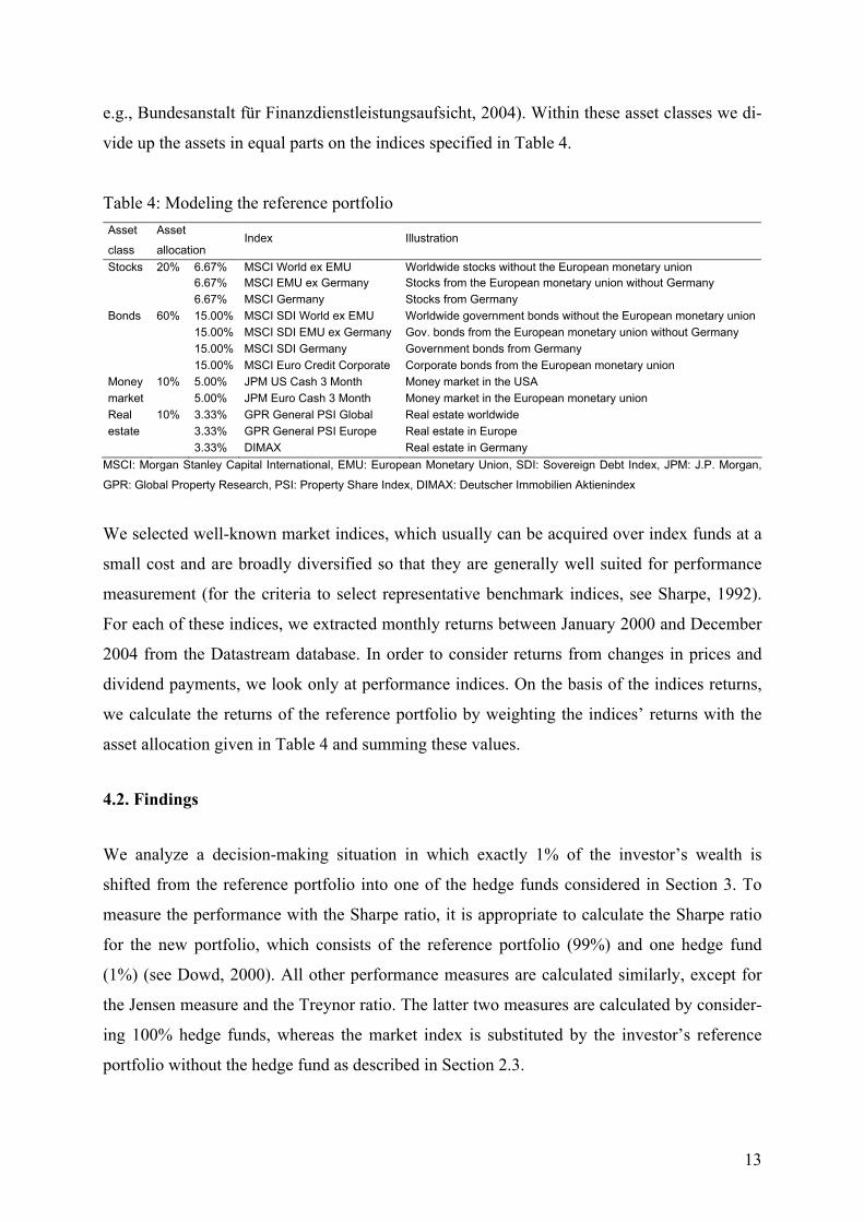
e.g., Bundesanstalt für Finanzdienstleistungsaufsicht, 2004). Within these asset classes we di-

vide up the assets in equal parts on the indices specified in Table 4.

Table 4: Modeling the reference portfolio

Asset

class

Asset

allocation Index Illustration

Stocks 20% 6.67% MSCI World ex EMU Worldwide stocks without the European monetary union

6.67% MSCI EMU ex Germany Stocks from the European monetary union without Germany

6.67% MSCI Germany Stocks from Germany

Bonds 60% 15.00% MSCI SDI World ex EMU Worldwide government bonds without the European monetary union

15.00% MSCI SDI EMU ex Germany Gov. bonds from the European monetary union without Germany

15.00% MSCI SDI Germany Government bonds from Germany

15.00% MSCI Euro Credit Corporate Corporate bonds from the European monetary union

Money 10% 5.00% JPM US Cash 3 Month Money market in the USA

market 5.00% JPM Euro Cash 3 Month Money market in the European monetary union

Real 10% 3.33% GPR General PSI Global Real estate worldwide

estate 3.33% GPR General PSI Europe Real estate in Europe

3.33% DIMAX Real estate in Germany

MSCI: Morgan Stanley Capital International, EMU: European Monetary Union, SDI: Sovereign Debt Index, JPM: J.P. Morgan,

GPR: Global Property Research, PSI: Property Share Index, DIMAX: Deutscher Immobilien Aktienindex

We selected well-known market indices, which usually can be acquired over index funds at a

small cost and are broadly diversified so that they are generally well suited for performance

measurement (for the criteria to select representative benchmark indices, see Sharpe, 1992).

For each of these indices, we extracted monthly returns between January 2000 and December

2004 from the Datastream database. In order to consider returns from changes in prices and

dividend payments, we look only at performance indices. On the basis of the indices returns,

we calculate the returns of the reference portfolio by weighting the indices’ returns with the

asset allocation given in Table 4 and summing these values.

4.2. Findings

We analyze a decision-making situation in which exactly 1% of the investor’s wealth is

shifted from the reference portfolio into one of the hedge funds considered in Section 3. To

measure the performance with the Sharpe ratio, it is appropriate to calculate the Sharpe ratio

for the new portfolio, which consists of the reference portfolio (99%) and one hedge fund

(1%) (see Dowd, 2000). All other performance measures are calculated similarly, except for

the Jensen measure and the Treynor ratio. The latter two measures are calculated by consider-

ing 100% hedge funds, whereas the market index is substituted by the investor’s reference

portfolio without the hedge fund as described in Section 2.3.

14

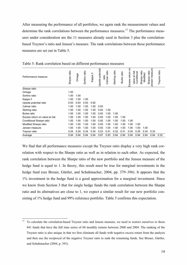
After measuring the performance of all portfolios, we again rank the measurement values and

determine the rank correlations between the performance measures.13 The performance meas-

ures under consideration are the 11 measures already used in Section 3 plus the correlation-

based Treynor’s ratio and Jensen’s measure. The rank correlations between these performance

measures are set out in Table 5.

Table 5: Rank correlation based on different performance measures

Performance measure

Sharpe ratio

Omega

Sortino ratio

Kappa 3

Upside potential

ratio

Calmar ratio

Sterling ratio

Burke ratio

Excess return on

value at risk

Conditional

Sharpe ratio

Modified

Sharpe ratio

Jensen measure

Treynor ratio

Sharpe ratio

Omega 1.00

Sortino ratio 1.00 1.00

Kappa 3 1.00 1.00 1.00

Upside potential ratio 0.93 0.93 0.93 0.92

Calmar ratio 1.00 1.00 1.00 1.00 0.93

Sterling ratio 1.00 1.00 1.00 1.00 0.93 1.00

Burke ratio 1.00 1.00 1.00 1.00 0.93 1.00 1.00

Excess return on value at risk 1.00 1.00 1.00 1.00 0.93 1.00 1.00 1.00

Conditional Sharpe ratio 1.00 1.00 1.00 1.00 0.92 1.00 1.00 1.00 1.00

Modified Sharpe ratio 1.00 1.00 1.00 1.00 0.93 1.00 1.00 1.00 1.00 1.00

Jensen measure 1.00 1.00 1.00 1.00 0.93 1.00 1.00 1.00 1.00 1.00 1.00

Treynor ratio 0.34 0.34 0.34 0.34 0.23 0.31 0.32 0.31 0.34 0.35 0.34 0.33

Average 0.94 0.94 0.94 0.94 0.87 0.93 0.94 0.94 0.94 0.94 0.94 0.94 0.32

We find that all performance measures except the Treynor ratio display a very high rank cor-

relation with respect to the Sharpe ratio as well as in relation to each other. As expected, the

rank correlation between the Sharpe ratio of the new portfolio and the Jensen measure of the

hedge fund is equal to 1. In theory, this result must be true for marginal investments in the

hedge fund (see Breuer, Gürtler, and Schuhmacher, 2004, pp. 379–396). It appears that the

1% investment in the hedge fund is a good approximation for a marginal investment. Since

we know from Section 3 that for single hedge funds the rank correlation between the Sharpe

ratio and its alternatives are close to 1, we expect a similar result for our new portfolio con-

sisting of 1% hedge fund and 99% reference portfolio. Table 5 confirms this expectation.

13 To calculate the correlation-based Treynor ratio and Jensen measure, we need to restrict ourselves to those

841 funds that have the full time series of 60 monthly returns between 2000 and 2004. The ranking of the

Treynor ratio is also unique in that we first eliminate all funds with negative excess return from the analysis

and then use the reciprocal of the negative Treynor ratio to rank the remaining funds. See Breuer, Gürtler,

and Schuhmacher (2004, p. 393).

15

Furthermore, we find that the rank correlation between the Treynor ratio and Jensen’s meas-

ure is relatively low. A possible explanation for this might be the fact that hedge funds are of-

ten more leveraged than other investment vehicles. Given this low rank correlation between

Jensen’s measure and the Treynor ratio and the high rank correlations between Jensen’s

measure and the remaining performance measures, it is clear that the rank correlations be-

tween the Treynor ratio and the remaining performance measures are relatively low as well.

We conclude that the Treynor ratio is not appropriate for performance analysis in this context

and exclude it from the following significance tests.

We used the test statistics described in Section 3.2 to check the statistical significance of the

rank correlations. The hypothesis of independence of the measurement series was again re-

jected for all correlation coefficients at a significance level of α = 0.01. We also again

checked the hypothesis that the rank correlation is smaller than a certain given number x. For

a significance level of α = 0.01, the hypothesis that the rank correlation is smaller than x is re-

jected for all x smaller than 0.916. We thus conclude that it does not much matter which

measure (except the Treynor ratio) is used to assess portfolio performance, as nearly all meas-

ures produce similar results.

4.3. Robustness of the findings

We examined the robustness of the results using the tests described in Section 3.3. None of

the changes listed in that section had a crucial influence on the results given in Section 4.2

(the results of these five tests are available upon request). However, for the modified decision-

making situation under consideration here, two additional robustness tests were made.

First, we altered the portion of hedge funds in the investor’s portfolio from between 1% and

10%. Table 6 shows the resulting rank correlations of the performance measures in relation to

the Sharpe ratio. For example, the third column of Table 6 shows rank correlations for the

situation where the investor wants to shift exactly 2% of his portfolio into hedge funds (we

also show the situation where the portfolio is invested 100% in hedge funds, which is the de-

cision-making situation discussed in Section 3).

16

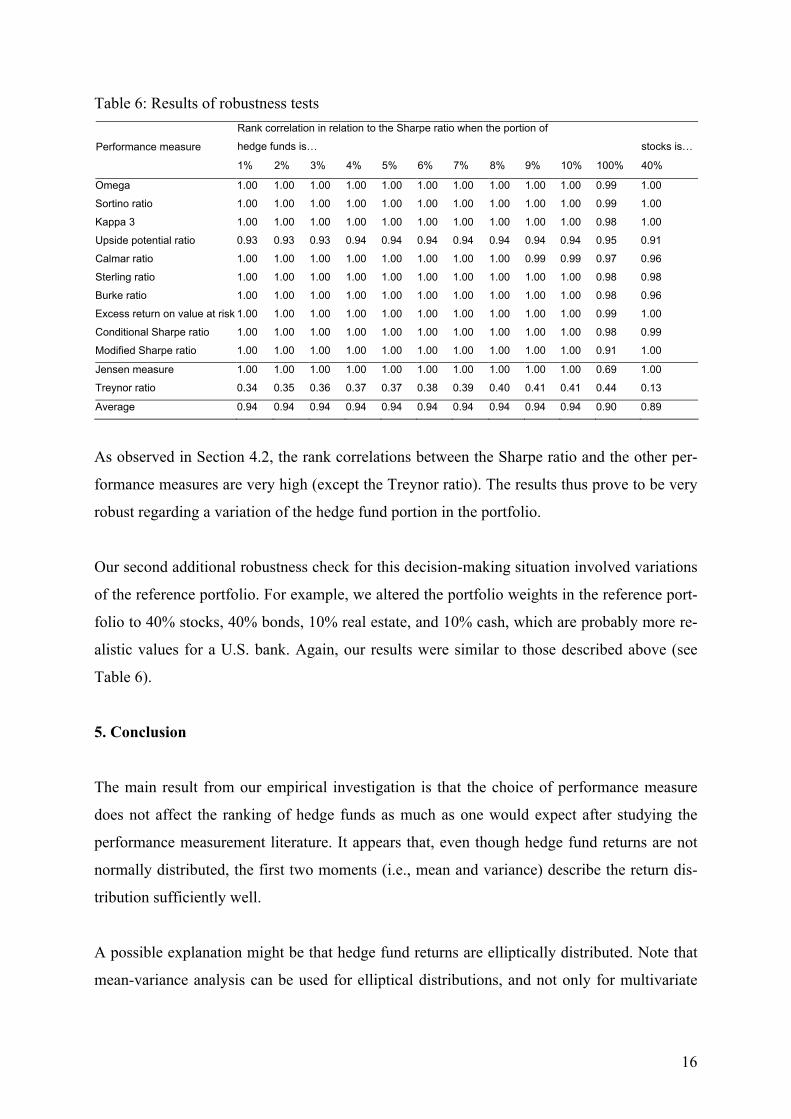
Table 6: Results of robustness tests

Rank correlation in relation to the Sharpe ratio when the portion of

hedge funds is… stocks is… Performance measure

1% 2% 3% 4% 5% 6% 7% 8% 9% 10% 100% 40%

Omega 1.00 1.00 1.00 1.00 1.00 1.00 1.00 1.00 1.00 1.00 0.99 1.00

Sortino ratio 1.00 1.00 1.00 1.00 1.00 1.00 1.00 1.00 1.00 1.00 0.99 1.00

Kappa 3 1.00 1.00 1.00 1.00 1.00 1.00 1.00 1.00 1.00 1.00 0.98 1.00

Upside potential ratio 0.93 0.93 0.93 0.94 0.94 0.94 0.94 0.94 0.94 0.94 0.95 0.91

Calmar ratio 1.00 1.00 1.00 1.00 1.00 1.00 1.00 1.00 0.99 0.99 0.97 0.96

Sterling ratio 1.00 1.00 1.00 1.00 1.00 1.00 1.00 1.00 1.00 1.00 0.98 0.98

Burke ratio 1.00 1.00 1.00 1.00 1.00 1.00 1.00 1.00 1.00 1.00 0.98 0.96

Excess return on value at risk 1.00 1.00 1.00 1.00 1.00 1.00 1.00 1.00 1.00 1.00 0.99 1.00

Conditional Sharpe ratio 1.00 1.00 1.00 1.00 1.00 1.00 1.00 1.00 1.00 1.00 0.98 0.99

Modified Sharpe ratio 1.00 1.00 1.00 1.00 1.00 1.00 1.00 1.00 1.00 1.00 0.91 1.00

Jensen measure 1.00 1.00 1.00 1.00 1.00 1.00 1.00 1.00 1.00 1.00 0.69 1.00

Treynor ratio 0.34 0.35 0.36 0.37 0.37 0.38 0.39 0.40 0.41 0.41 0.44 0.13

Average 0.94 0.94 0.94 0.94 0.94 0.94 0.94 0.94 0.94 0.94 0.90 0.89

As observed in Section 4.2, the rank correlations between the Sharpe ratio and the other per-

formance measures are very high (except the Treynor ratio). The results thus prove to be very

robust regarding a variation of the hedge fund portion in the portfolio.

Our second additional robustness check for this decision-making situation involved variations

of the reference portfolio. For example, we altered the portfolio weights in the reference port-

folio to 40% stocks, 40% bonds, 10% real estate, and 10% cash, which are probably more re-

alistic values for a U.S. bank. Again, our results were similar to those described above (see

Table 6).

5. Conclusion

The main result from our empirical investigation is that the choice of performance measure

does not affect the ranking of hedge funds as much as one would expect after studying the

performance measurement literature. It appears that, even though hedge fund returns are not

normally distributed, the first two moments (i.e., mean and variance) describe the return dis-

tribution sufficiently well.

A possible explanation might be that hedge fund returns are elliptically distributed. Note that

mean-variance analysis can be used for elliptical distributions, and not only for multivariate

17

normal distributions.14 Lhabitant (2004, p. 312) finds evidence for elliptically distributed

hedge funds returns. He observes a good statistical fit using the lognormal, the logistic, the

Weibull, or the generalized beta distribution, which all belong to the group of elliptical distri-

butions. For our data set we can confirm this finding.

What are the implications of our results? From a practical point of view, the choice of per-

formance measure does not have a crucial influence on the relative evaluation of hedge funds.

For example, in the portfolio context there are 98 hedge funds among the top 100 funds ac-

cording to an evaluation made using the Sharpe ratio, which are also among the top 100 funds

according to an evaluation made using Omega. Taking into account that the Sharpe ratio is the

best known (see Modigliani and Modigliani, 1997) and best understood performance measure

(see Lo, 2002), it might be considered superior to other performance measures from a practi-

tioner’s point of view.

Furthermore, from a theoretical point of view, the Sharpe ratio is consistent with expected

utility maximization under the assumption of elliptically distributed returns. Even without the

assumption of elliptically distributed returns, Fung and Hsieh (1999) have shown that mean-

variance analysis of hedge funds approximately preserves the ranking of preferences in stan-

dard utility functions.

We thus conclude that from a practical as well as from a theoretical point of view the Sharpe

ratio is adequate for analyzing hedge funds. As shown by Dowd (2000), the Sharpe ratio can

be used both when the hedge fund represents the entire risky investment and when it repre-

sents only a portion of the investor’s risky investment.

Acknowledgements

The authors thank the participants of the Financial Management Association European Con-

ference (Stockholm, June 2006), the Research Workshop on Portfolio Performance Evalua-

tion and Asset Management (Madrid, May 2006), the 9th Conference of the Swiss Society for

14 See Ingersoll (1987, p. 104). If the return vector of individual securities is elliptically distributed, then the re-

turn distribution of any portfolio from these securities is characterized by its expected return and variance. In

this case, the specific return distribution of the portfolio is of only secondary interest. Therefore, one does not

need distributions having stability or reproduction characteristics, like the normal distribution, in order to

found the mean-variance rule.

18

Financial Market Research (Zürich, April 2006), the 10th Symposium on Finance, Banking,

and Insurance (Karlsruhe, December 2005), and the German Operations Research Society

Conference 2005 (Bremen, September 2005). We are grateful to two anonymous referees and

to Giorgio P. Szegö, the editor of this journal. We also thank Florian Hach (ehedge) and Dee

Weber (CISDM) for providing the data.

References

Ackermann, C., McEnally, R., Ravenscraft, D., 1999. The Performance of Hedge Funds:

Risk, Return, and Incentives. Journal of Finance 54 (3), 833–874.

Agarwal, V., Naik, N. Y., 2004. Risk and Portfolio Decisions Involving Hedge Funds. Re-

view of Financial Studies 17 (1), 63–98.

Amin, G. S., Kat, H. M., 2003. Hedge Fund Performance 1990–2000: Do the Money Ma-

chines Really Add Value? Journal of Financial and Quantitative Analysis 38 (2), 251–274.

Bodie, Z., Kane, A., Marcus, A. J., 2005. Investments, 6th ed. McGraw Hill, New York.

Breuer, W., Gürtler, M., Schuhmacher, F., 2004. Portfoliomanagement I—Theoretische

Grundlagen und praktische Anwendungen. Gabler, Wiesbaden.

Brooks, C., Kat, H. M., 2002. The Statistical Properties of Hedge Fund Index Returns and

Their Implications for Investors. Journal of Alternative Investments, 5 (Fall), 26–44.

Bundesanstalt für Finanzdienstleistungsaufsicht, 2004. Jahresbericht der Bundesanstalt für Fi-

nanzdienstleistungsaufsicht ´03. Teil B, Bonn/Frankfurt am Main.

Burke, G., 1994. A Sharper Sharpe Ratio. Futures 23 (3), 56.

Chamberlain, G., 1983. A Characterization of the Distributions that Imply Mean-Variance

Utility Functions. Journal of Economic Theory 29 (1), 185–201.

Dowd, K., 2000. Adjusting for Risk: An Improved Sharpe Ratio. International Review of

Economics and Finance 9 (3), 209–222.

Eling, M., Schuhmacher, F., 2006. Hat die Wahl des Performancemaßes einen Einfluss auf

die Beurteilung von Hedgefonds-Indizes?, forthcoming in Kredit und Kapital 39 (3).

Favre, L., Galeano, J.-A., 2002. Mean-Modified Value-at-Risk Optimization with Hedge

Funds. Journal of Alternative Investments 5 (Fall), 21–25.

Fung, W., Hsieh, D. A., 1999. Is Mean-Variance Analysis Applicable to Hedge Funds? Eco-

nomic Letters 62 (1), 53–58.

Geman, H., Kharoubi, C., 2003. Hedge Funds Revisited: Distributional Characteristics, De-

pendence Structure and Diversification. Journal of Risk 5 (4), 55–73.

19

Gregoriou, G. N., Gueyie, J.-P., 2003. Risk-Adjusted Performance of Funds of Hedge Funds

Using a Modified Sharpe Ratio. Journal of Alternative Investments 6 (Winter), 77–83.

Ingersoll, J. E., 1987. Theory of Financial Decision Making. Rowman & Littlefield, Totowa,

NJ.

Jensen, M., 1968. The Performance of Mutual Funds in the Period 1945–1968. Journal of Fi-

nance 23 (2), 389–416.

Kao, D.-L., 2002. Battle for Alphas: Hedge Funds Versus Long-Only Portfolios. Financial

Analysts Journal 58 (March/April), 16–36.

Kaplan, P. D., Knowles, J. A., 2004. Kappa: A Generalized Downside Risk-Adjusted Perform-

ance Measure. Morningstar Associates and York Hedge Fund Strategies, January 2004.

Kat, H. M., 2003. 10 Things that Investors Should Know about Hedge Funds. Journal of

Wealth Management 5 (Spring), 72–81.

Kestner, L. N., 1996. Getting a Handle on True Performance. Futures 25 (1), 44–46.

Lhabitant, F.-S., 2004. Hedge Funds: Quantitative Insights. Wiley, Chichester.

Liang, B., 1999. On the Performance of Hedge Funds. Financial Analysts Journal 55

(July/August), 72–85.

Liang, B., 2000. Hedge Funds: The Living and the Dead. Journal of Financial and Quantita-

tive Analysis 35 (3), 309–326.

Lo, A. W., 2002. The Statistics of Sharpe Ratios. Financial Analysts Journal 58 (July/August),

36–52.

Mahdavi, M., 2004. Risk-Adjusted Return When Returns Are Not Normally Distributed: Ad-

justed Sharpe Ratio. Journal of Alternative Investments 6 (Spring), 47–57.

McFall Lamm, R., 2003. Asymmetric Returns and Optimal Hedge Fund Portfolios. Journal of

Alternative Investments 6 (Fall), 9–21.

Modigliani, F., Modigliani, L. 1997. Risk-Adjusted Performance—How to Measure it and

Why. Journal of Portfolio Management 23 (2), 45–54.

Pedersen, C. S., Rudholm-Alfvin, T., 2003. Selecting a Risk-Adjusted Shareholder Perform-

ance Measure. Journal of Asset Management 4 (3), 152–172.

Pfingsten, A., Wagner, P., Wolferink, C., 2004. An Empirical Investigation of the Rank Cor-

relation Between Different Risk Measures. Journal of Risk 6 (4), 55–74.

Rees, D. G., 1987. Foundation of Statistics. Chapman&Hall, London.

Schneeweis, T., Kazemi, H., Martin, G., 2002. Understanding Hedge Fund Performance: Re-

search Issues Revisited—Part I. Journal of Alternative Investments 5 (Winter), 6–22.

20

Scholz, H., Wilkens, M., 2003. Zur Relevanz von Sharpe Ratio und Treynor Ratio: Ein investor-

spezifisches Performancemaß. Zeitschrift für Bankrecht und Bankwirtschaft 15 (1), 1–8.

Shadwick, W. F., Keating, C., 2002. A Universal Performance Measure. Journal of Perform-

ance Measurement 6 (3), 59–84.

Sharma, M., 2004. A.I.R.A.P.—Alternative RAPMs for Alternative Investments. Journal of

Investment Management 2 (4), 106–129.

Sharpe, W. F., 1966. Mutual Fund Performance. Journal of Business 39 (1), 119–138.

Sharpe, W. F., 1992. Asset Allocation: Management Style and Performance Measurement.

Journal of Portfolio Management 18 (Winter), 7–19.

Sortino, F. A., van der Meer, R., 1991. Downside Risk. Journal of Portfolio Management 17

(Spring), 27–31.

Sortino, F. A., van der Meer, R., Plantinga, A., 1999. The Dutch Triangle. Journal of Portfolio

Management 26(Fall), 50–58.

Treynor, J. L., 1965. How to Rate Management of Investment Funds. Harvard Business Re-

view 43 (1), 63–75.

Van, George P., 2005. Hedge Fund Demand and Capacity 2005–2015. Van Hedge Fund Ad-

visors, August 2005.

Young, T. W., 1991. Calmar Ratio: A Smoother Tool. Futures 20 (1), 40.