Embed Size (px)
Citation preview
World Leader in Rating Technology
OFFSHORE RACING CONGRESS
ORC VPP Documenation
2015

Copyright © 2015 Offshore Racing Congress.
All rights reserved. Reproduction in whole or in part is
only with the permission of the Offshore Racing Congress.
Cover picture: Wind tunnel testing at Politecnico Milano
by courtesy Dobbs Davis
Section 1 Page 3
1 Background
The following document describes the methods and formulations used by the Offshore Racing
Congress (ORC) Velocity Prediction Program (VPP).
The ORC VPP is the program used to calculate racing yacht handicaps based on a mathematical model
of the physical processes embodied in a sailing yacht. This approach to handicapping was first
developed in 1978. The H. Irving Pratt Ocean Racing Handicapping project created a handicap system
which used a mathematical model of hull and rig performance to predict sailing speeds and thereby
produce a time on distance handicap system. This computational approach to yacht handicapping was
of course only made possible by the advent of desktop computing capability.
The first 2 papers describing the project were presented to the Chesapeake Sailing Yacht Symposium
(CSYS) in 19791. This work resulted in the MHS system that was used in the United States. The
aerodynamic model was subsequently revised by George Hazen2 and the hydrodynamic model was
refined over time as the Delft Systematic Yacht Hull Series was expanded3.
Other research was documented in subsequent CSYS proceedings: sail formulations (20014 and
20035), and hull shape effects (20036). Papers describing research have also been published in the
HISWA symposia on sail research (20087).
In 1986 the current formulations of the IMS were documented by Charlie Poor8, and this was updated
in 19999. The 1999 CSYS paper was used a basis for this document, with members of the ITC
contributing the fruits of their labours over the last 10 years as the ORC carried forward the work of
maintaining an up-to-date handicapping system that is based on the physics of a sailing yacht.
1 “A summary of the H. Irving Pratt Ocean race Handicapping Project”. (Kerwin, J.E, & Newman, J.N.) “The Measurement
Handicapping System of USYRU” (Stromhmeier, D.D) 2 Hazen, G., “A Model of Sail Aerodynamics for Diverse Rig Types,” New England Sailing Yacht Symposium. New London, CT,
1980. 3 1993, CSYS The Delft Systematic Yacht Hull (Series II) Experiments. Gerritsma, Prof. ir. J., Keuning, Ir. J., and Onnink, A. R. 4 Aerodynamic Performance of Offwind Sails Attached to Sprits. Robert Ranzenbach and Jim Teeters 5 Changes to Sail Aerodynamics in the IMS Rule Jim Teeters, Robert Ranzenbach and Martyn Prince 6 Aerodynamic Performance of Offwind Sails Attached to Sprits. Robert Ranzenbach and Jim Teeters 7 Fossati F., Claughton A., Battistin D., Muggiasca S.: “Changes and Development to Sail Aerodynamics in the ORC International
Rule” – 20th HISWA Symposium, Amsterdam, 2008 8 “The IMS, a description of the new international rating system” Washington DC 1986 9 Claughton, A., “Developments in the IMS VPP Formulations,” SNAME 14th CSYS, Annapolis, MD, 1999.
Section 1 Page 4
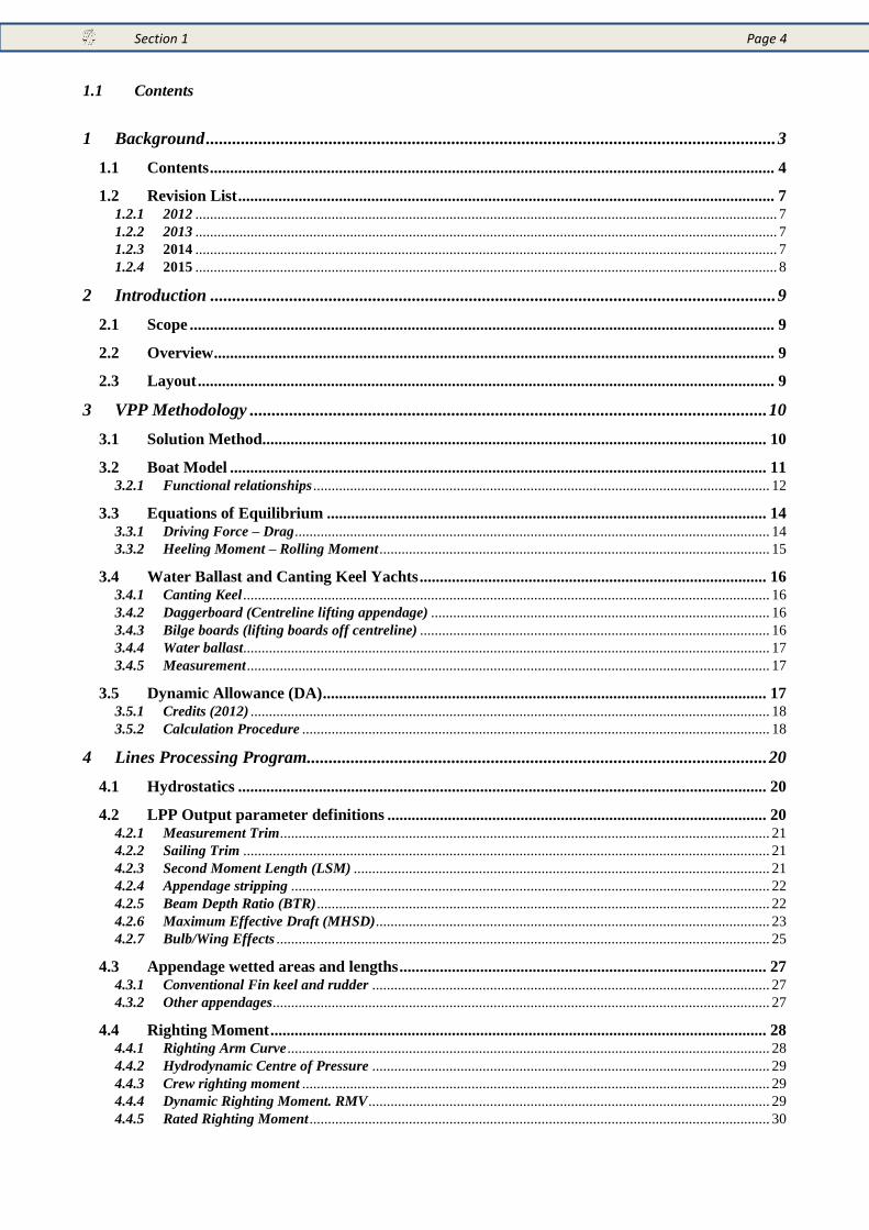
1.1 Contents
1 Background .................................................................................................................................. 3
1.1 Contents ............................................................................................................................................ 4
1.2 Revision List ..................................................................................................................................... 7 1.2.1 2012 .............................................................................................................................................................. 7 1.2.2 2013 .............................................................................................................................................................. 7 1.2.3 2014 .............................................................................................................................................................. 7 1.2.4 2015 .............................................................................................................................................................. 8
2 Introduction ................................................................................................................................. 9
2.1 Scope ................................................................................................................................................. 9
2.2 Overview ........................................................................................................................................... 9
2.3 Layout ............................................................................................................................................... 9
3 VPP Methodology ...................................................................................................................... 10
3.1 Solution Method ............................................................................................................................. 10
3.2 Boat Model ..................................................................................................................................... 11 3.2.1 Functional relationships ............................................................................................................................ 12
3.3 Equations of Equilibrium ............................................................................................................. 14 3.3.1 Driving Force – Drag ................................................................................................................................. 14 3.3.2 Heeling Moment – Rolling Moment .......................................................................................................... 15
3.4 Water Ballast and Canting Keel Yachts ...................................................................................... 16 3.4.1 Canting Keel ............................................................................................................................................... 16 3.4.2 Daggerboard (Centreline lifting appendage) ............................................................................................ 16 3.4.3 Bilge boards (lifting boards off centreline) ............................................................................................... 16 3.4.4 Water ballast............................................................................................................................................... 17 3.4.5 Measurement .............................................................................................................................................. 17
3.5 Dynamic Allowance (DA) .............................................................................................................. 17 3.5.1 Credits (2012) ............................................................................................................................................. 18 3.5.2 Calculation Procedure ............................................................................................................................... 18
4 Lines Processing Program......................................................................................................... 20
4.1 Hydrostatics ................................................................................................................................... 20
4.2 LPP Output parameter definitions .............................................................................................. 20 4.2.1 Measurement Trim ..................................................................................................................................... 21 4.2.2 Sailing Trim ............................................................................................................................................... 21 4.2.3 Second Moment Length (LSM) ................................................................................................................. 21 4.2.4 Appendage stripping .................................................................................................................................. 22 4.2.5 Beam Depth Ratio (BTR) ........................................................................................................................... 22 4.2.6 Maximum Effective Draft (MHSD) ........................................................................................................... 23 4.2.7 Bulb/Wing Effects ...................................................................................................................................... 25
4.3 Appendage wetted areas and lengths ........................................................................................... 27 4.3.1 Conventional Fin keel and rudder ............................................................................................................ 27 4.3.2 Other appendages ....................................................................................................................................... 27
4.4 Righting Moment ........................................................................................................................... 28 4.4.1 Righting Arm Curve ................................................................................................................................... 28 4.4.2 Hydrodynamic Centre of Pressure ............................................................................................................ 29 4.4.3 Crew righting moment ............................................................................................................................... 29 4.4.4 Dynamic Righting Moment. RMV ............................................................................................................. 29 4.4.5 Rated Righting Moment ............................................................................................................................. 30
Section 1 Page 5
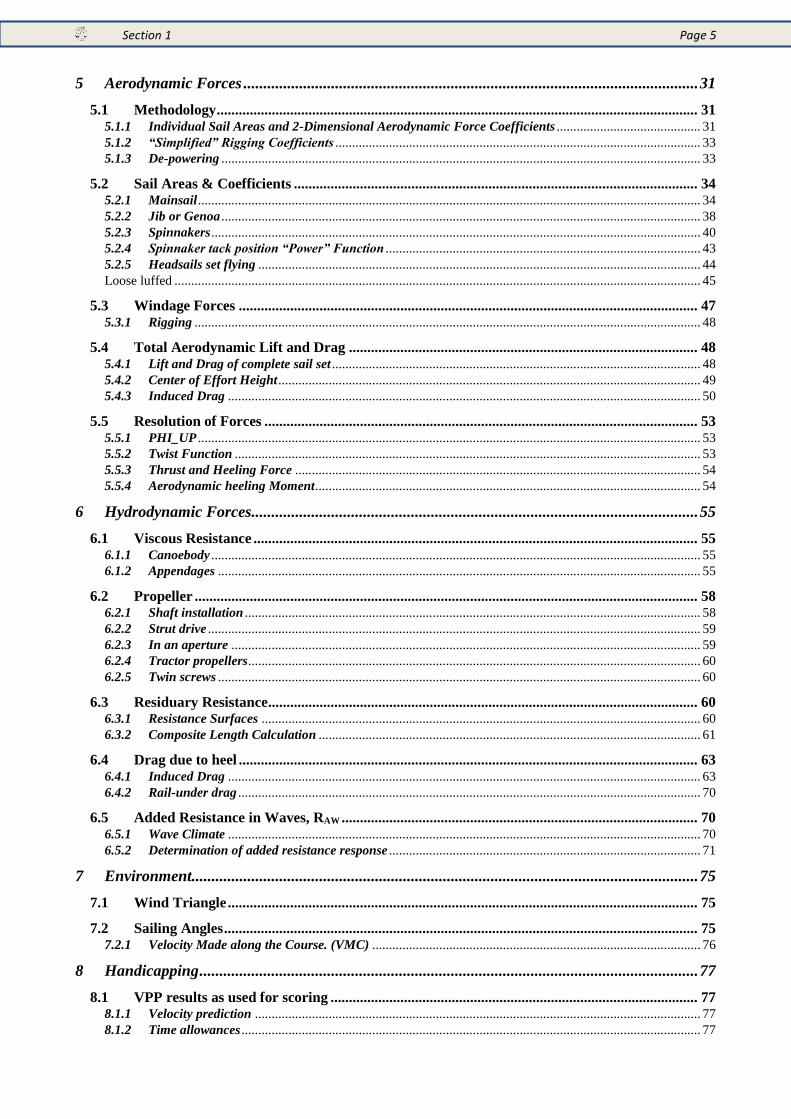
5 Aerodynamic Forces .................................................................................................................. 31
5.1 Methodology ................................................................................................................................... 31 5.1.1 Individual Sail Areas and 2-Dimensional Aerodynamic Force Coefficients ........................................... 31 5.1.2 “Simplified” Rigging Coefficients ............................................................................................................. 33 5.1.3 De-powering ............................................................................................................................................... 33
5.2 Sail Areas & Coefficients .............................................................................................................. 34 5.2.1 Mainsail ...................................................................................................................................................... 34 5.2.2 Jib or Genoa ............................................................................................................................................... 38 5.2.3 Spinnakers .................................................................................................................................................. 40 5.2.4 Spinnaker tack position “Power” Function .............................................................................................. 43 5.2.5 Headsails set flying .................................................................................................................................... 44 Loose luffed ............................................................................................................................................................. 45
5.3 Windage Forces ............................................................................................................................. 47 5.3.1 Rigging ....................................................................................................................................................... 48
5.4 Total Aerodynamic Lift and Drag ............................................................................................... 48 5.4.1 Lift and Drag of complete sail set .............................................................................................................. 48 5.4.2 Center of Effort Height .............................................................................................................................. 49 5.4.3 Induced Drag ............................................................................................................................................. 50
5.5 Resolution of Forces ...................................................................................................................... 53 5.5.1 PHI_UP ...................................................................................................................................................... 53 5.5.2 Twist Function ........................................................................................................................................... 53 5.5.3 Thrust and Heeling Force ......................................................................................................................... 54 5.5.4 Aerodynamic heeling Moment ................................................................................................................... 54
6 Hydrodynamic Forces ................................................................................................................ 55
6.1 Viscous Resistance ......................................................................................................................... 55 6.1.1 Canoebody .................................................................................................................................................. 55 6.1.2 Appendages ................................................................................................................................................ 55
6.2 Propeller ......................................................................................................................................... 58 6.2.1 Shaft installation ........................................................................................................................................ 58 6.2.2 Strut drive ................................................................................................................................................... 59 6.2.3 In an aperture ............................................................................................................................................ 59 6.2.4 Tractor propellers ....................................................................................................................................... 60 6.2.5 Twin screws ................................................................................................................................................ 60
6.3 Residuary Resistance ..................................................................................................................... 60 6.3.1 Resistance Surfaces ................................................................................................................................... 60 6.3.2 Composite Length Calculation .................................................................................................................. 61
6.4 Drag due to heel ............................................................................................................................. 63 6.4.1 Induced Drag ............................................................................................................................................. 63 6.4.2 Rail-under drag .......................................................................................................................................... 70
6.5 Added Resistance in Waves, RAW ................................................................................................. 70 6.5.1 Wave Climate ............................................................................................................................................. 70 6.5.2 Determination of added resistance response ............................................................................................. 71
7 Environment............................................................................................................................... 75
7.1 Wind Triangle ................................................................................................................................ 75
7.2 Sailing Angles ................................................................................................................................. 75 7.2.1 Velocity Made along the Course. (VMC) .................................................................................................. 76
8 Handicapping ............................................................................................................................. 77
8.1 VPP results as used for scoring .................................................................................................... 77 8.1.1 Velocity prediction ..................................................................................................................................... 77 8.1.2 Time allowances ......................................................................................................................................... 77
Section 1 Page 6
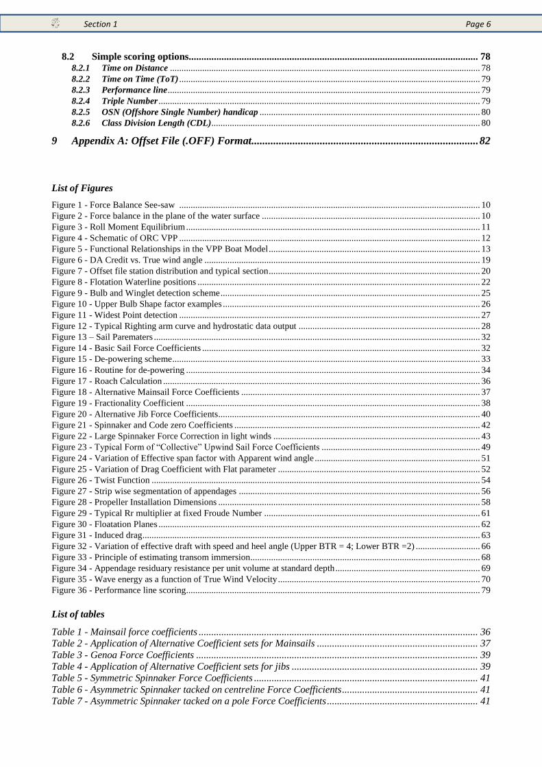
8.2 Simple scoring options................................................................................................................... 78 8.2.1 Time on Distance ....................................................................................................................................... 78 8.2.2 Time on Time (ToT) ................................................................................................................................... 79 8.2.3 Performance line ........................................................................................................................................ 79 8.2.4 Triple Number ............................................................................................................................................ 79 8.2.5 OSN (Offshore Single Number) handicap ................................................................................................ 80 8.2.6 Class Division Length (CDL)..................................................................................................................... 80
9 Appendix A: Offset File (.OFF) Format ................................................................................... 82
List of Figures
Figure 1 - Force Balance See-saw ................................................................................................................................... 10
Figure 2 - Force balance in the plane of the water surface ............................................................................................... 10
Figure 3 - Roll Moment Equilibrium ................................................................................................................................ 11
Figure 4 - Schematic of ORC VPP ................................................................................................................................... 12
Figure 5 - Functional Relationships in the VPP Boat Model ............................................................................................ 13
Figure 6 - DA Credit vs. True wind angle ........................................................................................................................ 19
Figure 7 - Offset file station distribution and typical section ............................................................................................ 20
Figure 8 - Flotation Waterline positions ........................................................................................................................... 22
Figure 9 - Bulb and Winglet detection scheme ................................................................................................................. 25
Figure 10 - Upper Bulb Shape factor examples ................................................................................................................ 26
Figure 11 - Widest Point detection ................................................................................................................................... 27
Figure 12 - Typical Righting arm curve and hydrostatic data output ............................................................................... 28
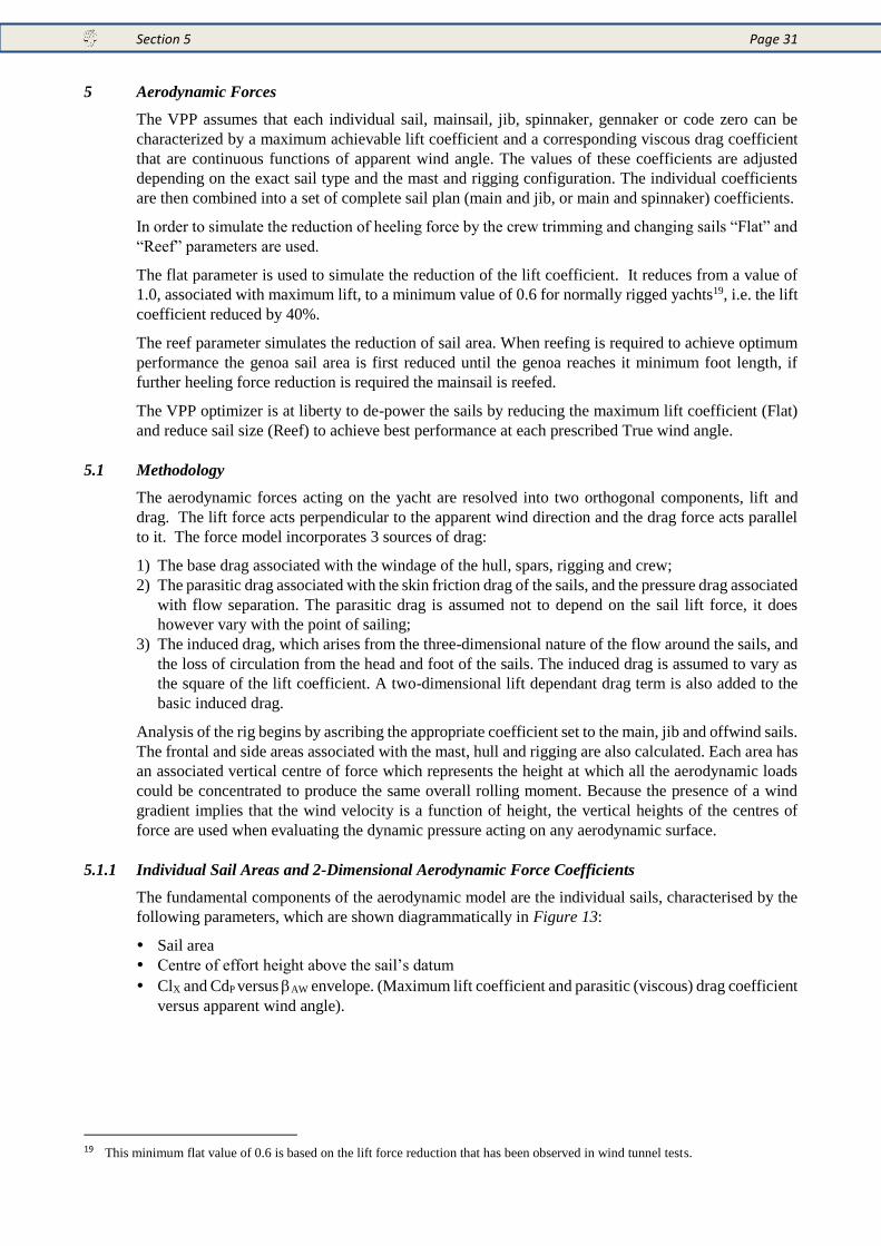
Figure 13 – Sail Parematers .............................................................................................................................................. 32
Figure 14 - Basic Sail Force Coefficients ......................................................................................................................... 32
Figure 15 - De-powering scheme ...................................................................................................................................... 33
Figure 16 - Routine for de-powering ................................................................................................................................ 34
Figure 17 - Roach Calculation .......................................................................................................................................... 36
Figure 18 - Alternative Mainsail Force Coefficients ........................................................................................................ 37
Figure 19 - Fractionality Coefficient ................................................................................................................................ 38
Figure 20 - Alternative Jib Force Coefficients.................................................................................................................. 40
Figure 21 - Spinnaker and Code zero Coefficients ........................................................................................................... 42
Figure 22 - Large Spinnaker Force Correction in light winds .......................................................................................... 43
Figure 23 - Typical Form of “Collective” Upwind Sail Force Coefficients ..................................................................... 49
Figure 24 - Variation of Effective span factor with Apparent wind angle ........................................................................ 51
Figure 25 - Variation of Drag Coefficient with Flat parameter ........................................................................................ 52
Figure 26 - Twist Function ............................................................................................................................................... 54
Figure 27 - Strip wise segmentation of appendages ......................................................................................................... 56
Figure 28 - Propeller Installation Dimensions .................................................................................................................. 58
Figure 29 - Typical Rr multiplier at fixed Froude Number .............................................................................................. 61
Figure 30 - Floatation Planes ............................................................................................................................................ 62
Figure 31 - Induced drag ................................................................................................................................................... 63
Figure 32 - Variation of effective draft with speed and heel angle (Upper BTR = 4; Lower BTR =2) ............................ 66
Figure 33 - Principle of estimating transom immersion.................................................................................................... 68
Figure 34 - Appendage residuary resistance per unit volume at standard depth ............................................................... 69
Figure 35 - Wave energy as a function of True Wind Velocity ........................................................................................ 70
Figure 36 - Performance line scoring................................................................................................................................ 79
List of tables
Table 1 - Mainsail force coefficients ............................................................................................................... 36
Table 2 - Application of Alternative Coefficient sets for Mainsails ................................................................ 37
Table 3 - Genoa Force Coefficients ................................................................................................................ 39
Table 4 - Application of Alternative Coefficient sets for jibs .......................................................................... 39
Table 5 - Symmetric Spinnaker Force Coefficients ......................................................................................... 41
Table 6 - Asymmetric Spinnaker tacked on centreline Force Coefficients ...................................................... 41
Table 7 - Asymmetric Spinnaker tacked on a pole Force Coefficients ............................................................ 41
Section 1 Page 7
Table 8 - Code Zero force coefficients ............................................................... Error! Bookmark not defined.
Table 9 - Windage force model........................................................................................................................ 47
Table 10 - Calculated PHI_UP values ............................................................................................................ 53
Table 11 - Appendage Cf. values used in the VPP .......................................................................................... 56
Table 12 - L calculation scheme ...................................................................................................................... 62
Table 13 - Added Resistance in Waves; parametric limits and base values .................................................... 72
Table 14 - VPP True wind angle and wind speed matrix ................................................................................ 75
Table 15 - Velocity prediction printed on the 1st page of the ORC International certificate ......................... 77
Table 16 - Time Allowances and Selected Courses on the 1st page of the ORC International certificate ..... 77
Table 17 - Simple scoring options on ORC International & ORC Club certificate ........................................ 78
Table 18 - Time allowance weighting table ..................................................................................................... 80
1.2 Revision List
1.2.1 2012
Section Change
3.5.1 Modified Dynamic Allowance terms
5.2.3.3 Modified force coefficients for large spinnakers in light airs.
5.4.2.1 Add Jib Twist effect on sail plan vertical centre of pressure
6.3.11 Include effect of crew longitudinal position on Immersed transom resistance.
8.2.5 Offshore Single Number Handicap added
1.2.2 2013
Section Change
Fig 5 Updated
Equation 2 Revised
4.2.2 Removed
4.2.2.2 Removed
5.2.1.1 Roach Calculation.
5.2.3.2 Asymmetric on CL coefficients changed
5.2.3.3 Shape Function modified
5.2.3 Blanketing Function deleted.
5.2.5.2 Power Function Modified
6.1.1 Viscous resistance of canoe body modified
6.3 Residuary resistance Formulation Modified
6.3 Transom overhang deleted
6.3 SBF factor deleted
6.4 Heel Drag modified
1.2.3 2014
Section Change
3.4.4 Added configuration of water ballast with canting keel
4.2.6.2 Possibility to rate boats with double fixed keel with bulb
4.4.5 RM Bias for ORC Club boats not inclined
5.2.3.5 Reduced maximum heel angle with spinnaker
5.2.4 Fine tuning of Power function
5.2.5 Headsails set flying
5.4.3.2 Cd-Cl2 mutliplier in the aero model
6.3.1 Fine tuning of Residuary Resistance
6.4.1 Fine tuning of canting keel with double canards
6.4.2 Reduced maximum heel angle with spinnaker
6.5.2.1 Carbon mast elastic modulus modified
6.5.2.1 Titanium and carbon stanchions allowance
8.2.5 Offshore Single Number fine tuning
Section 1 Page 8
1.2.4 2015
Section Change
4.4.5 New formula for the rated righting moment
5.2.2.2 Blending of battened genoa and jib aero coefficients
5.2.5.2 Change of default sail area for headsail set flying
5.2.5.4 New set of aero coefficients for headsail set flying with tight luff
6.2.1 Update on folding and feathering propeller treatment
8.3 New Class Division Length (CDL) definition
Section 2 Page 9
2 Introduction
2.1 Scope
The following document is a companion to the ORC Rating Rules and IMS (International
Measurement System). The document provides a summary of the physics and computational processes
that lie behind the calculation of sailing speeds and corresponding time allowances (seconds/mile).
The current ORC handicap system comprises 3 separate elements:
1) The IMS measurement procedure whereby the physical shape of the hull and appendages are
defined, along with dimensions of mast, sails, etc.
2) A performance prediction procedure based on (1) a lines processing procedure which determines
the parametric inputs used by the Velocity Prediction Program (VPP) to predict sailing speed on
different points of sailing, in different wind speeds with different sails set.
3) A race management system whereby the results of (2) are applied to offer condition-specific race
handicapping.
This document describes the methodology of the equations used to calculate the forces produced by
the hull, appendages, and sails, and how these are combined in the VPP.
2.2 Overview
Predicting the speed of a sailing yacht from its physical dimensions alone is a complex task,
particularly when constrained by the need to do it in the “general case” using software that is robust
enough to be run routinely by rating offices throughout the world. Nevertheless this is what the ORC
Rating system aims to do. The only absolute record of the VPP (and companion Lines Processing
Program (LPP)) is the FORTRAN source code, so it is a difficult matter for a layman to determine
either the intent or underlying methodology by inspection of this code.
The purpose of this document is to describe the physical basis of the methods used to predict the forces
on a sailing yacht rig and hull, and to define the formulations (equations) used by the VPP to
encapsulate the physical model.
In order to do this the document has been set out to first layout the broadest view of the process,
gradually breaking the problem down into its constituent parts, so that ultimately the underlying
equations of the VPP can be presented.
2.3 Layout
The document is arranged in 6 sections:
Section 3 describes the methods by which the velocity prediction is carried out and the fundamental
force balances inherent in solving the problem are laid out. Following this an overview of the “boat
model” is presented, whereby the elements of the aerodynamic and hydrodynamic model are
described.
Section 4 describes how the hull shape parameters are pre-processed to determine the parameters
that are used in the hydrodynamic force model described in Section 8.
Section 5 describes how the yacht’s environment is characterized in terms of the incident wind
field experienced by the sails.
Section 6 describes how the VPP results are presented as a rating certificate.
Section 7 describes the methods used to predict the aerodynamic forces produced by the mast, sails,
and above-water part of the hull.
Section 8 describes how the hydrodynamic drag and lift of the hull and appendages are calculated.
Section 3 Page 10
3 VPP Methodology
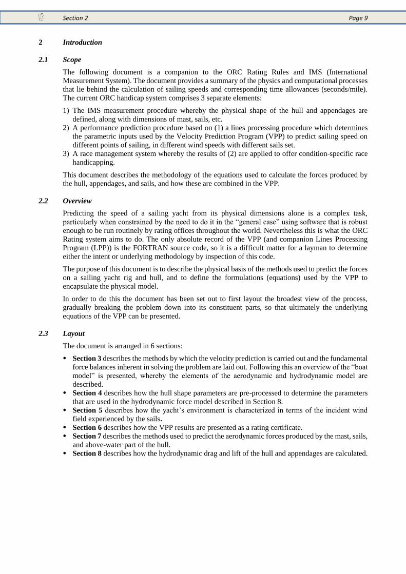
The VPP has a two-part structure comprised of the solution algorithm and the boat model. The solution
algorithm must find an equilibrium condition for each point of sailing where:
a) the driving force from the sails matches the hull and aerodynamic drag, and
b) the heeling moment from the rig is matched by the righting moment from the hull.
i.e. balance the seesaw in Figure 110, and optimize the sail controls (reef and flat) to produce the
maximum speed at each true wind angle.
Figure 1 - Force Balance See-saw
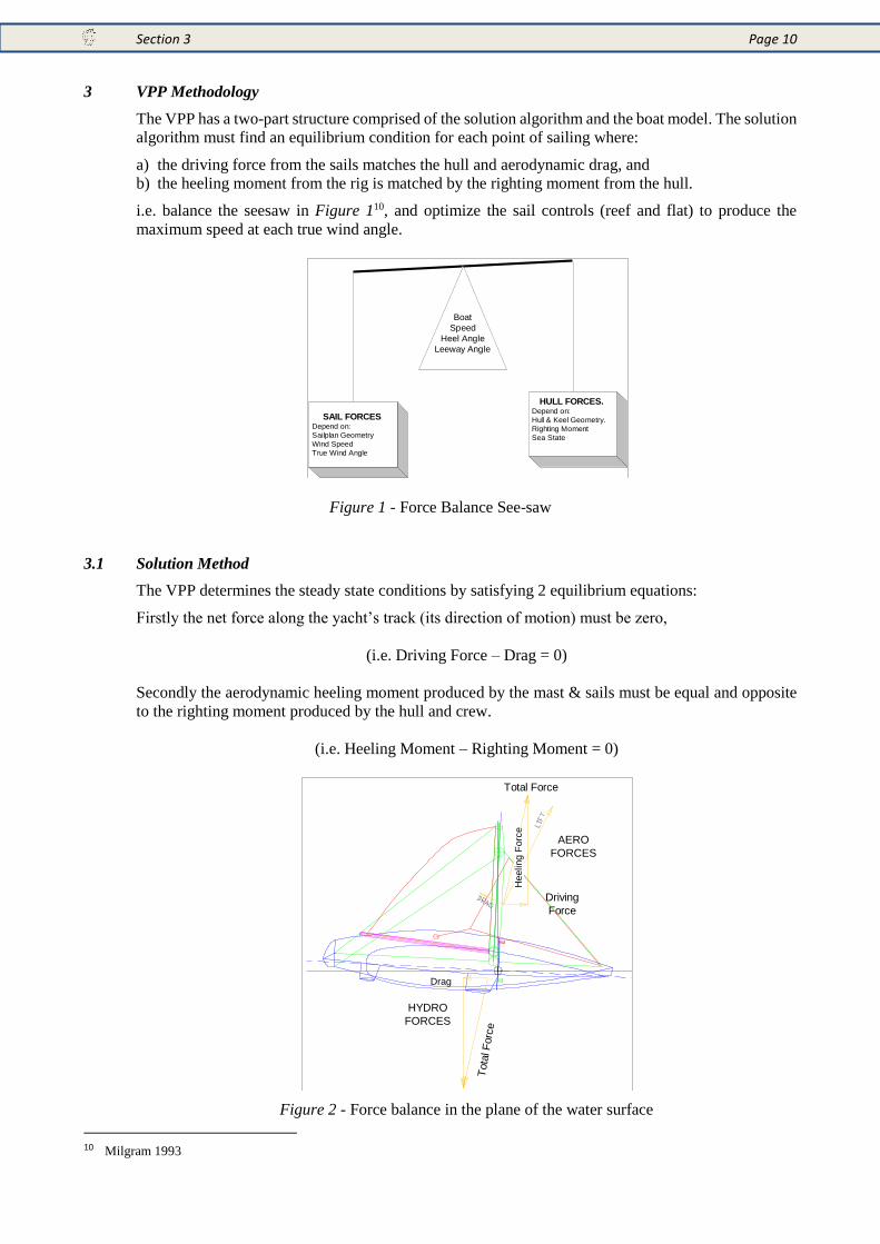
3.1 Solution Method
The VPP determines the steady state conditions by satisfying 2 equilibrium equations:
Firstly the net force along the yacht’s track (its direction of motion) must be zero,
(i.e. Driving Force – Drag = 0)
Secondly the aerodynamic heeling moment produced by the mast & sails must be equal and opposite
to the righting moment produced by the hull and crew.
(i.e. Heeling Moment – Righting Moment = 0)
Figure 2 - Force balance in the plane of the water surface
10 Milgram 1993
Boat
Speed
Heel Angle
Leeway Angle
SAIL FORCESDepend on:
Sailplan Geometry
Wind Speed
True Wind Angle
HULL FORCES.Depend on:
Hull & Keel Geometry.
Righting Moment
Sea State
Driving
Force
Drag
AERO
FORCES
HYDRO
FORCES
Heeling F
orc
e
Total Force
Tota
l F
orc
e
Section 3 Page 11
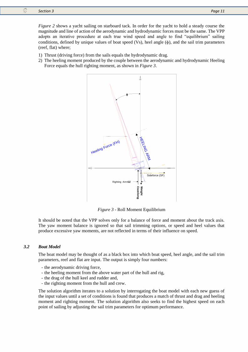
Figure 2 shows a yacht sailing on starboard tack. In order for the yacht to hold a steady course the
magnitude and line of action of the aerodynamic and hydrodynamic forces must be the same. The VPP
adopts an iterative procedure at each true wind speed and angle to find “equilibrium” sailing
conditions, defined by unique values of boat speed (Vs), heel angle (), and the sail trim parameters
(reef, flat) where;
1) Thrust (driving force) from the sails equals the hydrodynamic drag.
2) The heeling moment produced by the couple between the aerodynamic and hydrodynamic Heeling
Force equals the hull righting moment, as shown in Figure 3.
Figure 3 - Roll Moment Equilibrium
It should be noted that the VPP solves only for a balance of force and moment about the track axis.
The yaw moment balance is ignored so that sail trimming options, or speed and heel values that
produce excessive yaw moments, are not reflected in terms of their influence on speed.
3.2 Boat Model
The boat model may be thought of as a black box into which boat speed, heel angle, and the sail trim
parameters, reef and flat are input. The output is simply four numbers:
- the aerodynamic driving force,
- the heeling moment from the above water part of the hull and rig,
- the drag of the hull keel and rudder and,
- the righting moment from the hull and crew.
The solution algorithm iterates to a solution by interrogating the boat model with each new guess of
the input values until a set of conditions is found that produces a match of thrust and drag and heeling
moment and righting moment. The solution algorithm also seeks to find the highest speed on each
point of sailing by adjusting the sail trim parameters for optimum performance.
Heeling Force (FH)
Sideforce (SF)
We
igh
t
Righting Arm GZ
HE
ELIN
G A
RM
Bu
oy
an
cy
Section 3 Page 12
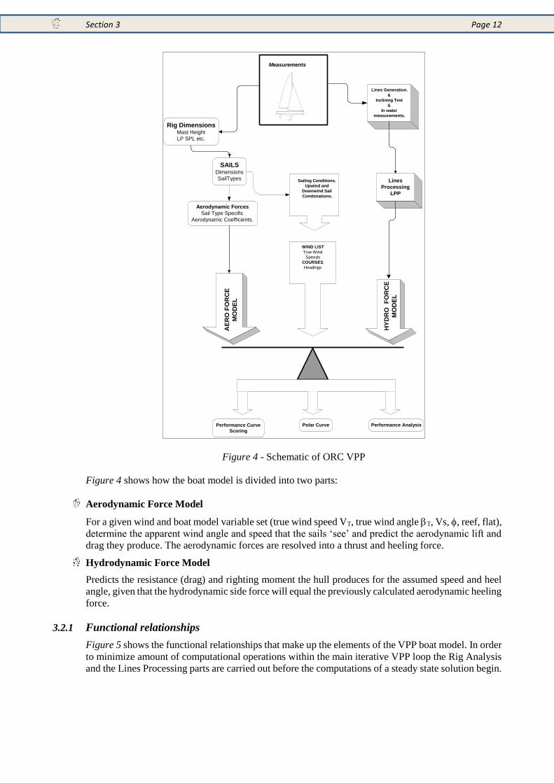
Figure 4 - Schematic of ORC VPP
Figure 4 shows how the boat model is divided into two parts:
Aerodynamic Force Model
For a given wind and boat model variable set (true wind speed VT, true wind angle T, Vs, , reef, flat),
determine the apparent wind angle and speed that the sails ‘see’ and predict the aerodynamic lift and
drag they produce. The aerodynamic forces are resolved into a thrust and heeling force.
Hydrodynamic Force Model
Predicts the resistance (drag) and righting moment the hull produces for the assumed speed and heel
angle, given that the hydrodynamic side force will equal the previously calculated aerodynamic heeling
force.
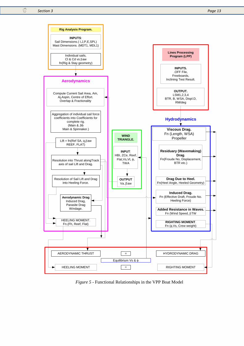
3.2.1 Functional relationships
Figure 5 shows the functional relationships that make up the elements of the VPP boat model. In order
to minimize amount of computational operations within the main iterative VPP loop the Rig Analysis
and the Lines Processing parts are carried out before the computations of a steady state solution begin.
WIND LIST
True Wind
Speeds
COURSES
Headings
Sailing Conditions.
Upwind and
Downwind Sail
Combinations.
AE
RO
FO
RC
E
MO
DE
L
HY
DR
O
FO
RC
E
MO
DE
L
SAILSDimensions
SailTypes
Aerodynamic Forces
Sail Type Specific
Aerodynamic Coefficients.
Rig DimensionsMast Height
LP SPL etc.
Lines
Processing
LPP
Lines Generation.
&
Inclining Test
&
In water
measurements.
Performance Curve
Scoring
Polar Curve Performance Analysis
Measurements
Section 3 Page 13
Figure 5 - Functional Relationships in the VPP Boat Model
AERODYNAMIC THRUST = HYDRODYNAMIC DRAG
Resolution into Thrust alongTrack
axis of sail Lift and Drag.
Lift = fn(Ref SA, q,aw
REEF, FLAT)
Individual sails,
Cl & Cd vs aw
fn(Rig & Stay geometry)
Aerodynamic Drag
Induced Drag,
Parasite Drag
Windage.
Viscous Drag.Fn (Length, WSA)
Residuary (Wavemaking)
Drag.
Fn(Froude No, Displacement,
BTR etc.)
Drag Due to Heel.Fn(Heel Angle, Heeled Geometry)
Induced Drag.Fn (Effective Draft, Froude No.
Heeling Force)
Added Resistance in Waves.Fn (Wind Speed, TW
Lines Processing
Program (LPP)
INPUTS.
.OFF File,
Freeboards,
Inclining Test Result.
OUTPUT.
LSM1,2,3,4
BTR, B, WSA, Displ.D,
RM/deg
Rig Analysis Program.
INPUTS:
Sail Dimensions.( I,J,P,E,SPL)
Mast Dimensions. (MDT1, MDL1)
Compute Current Sail Area, Am,
Aj,Aspin, Centre of Effort.
Overlap & Fractionality
WIND
TRIANGLE.
INPUT:
HBI, ZCe, Reef,
Flat,Vs,Vt, ,
TWA
OUTPUT
Va,aw
HEELING MOMENT RIGHTING MOMENT=
Resolution of Sail Lift and Drag
into Heeling Force.
RIGHTING MOMENT.
Fn (Vs, Crew weight)
HEELING MOMENT.
Fn.(Fh, Reef, Flat)
Equilibrium Vs &
Aerodynamics
Hydrodynamics
Aggregation of individual sail force
coefficients into Coefficients for
complete rig.
(Main & Jib
Main & Spinnaker.) Viscous Drag.
Fn (Length, WSA)
Propeller
Section 3 Page 14
3.2.1.1 Rig Analysis Program
The Rig Analysis Program takes the measured sail and rig dimensions and calculates the areas and
centres of effort for the mainsail, jib and spinnaker. Originally the Rig Analysis Program used the force
coefficients for each individual sail to calculate a “collective” set of aerodynamic force coefficients
for the rig in an upwind and downwind configuration. This collective table of lift and drag coefficients
at each apparent wind angle is interrogated by the solution algorithm during each iteration as the
program works towards an equilibrium sailing condition.
More recently11 for the upwind sailing configurations the calculation of the “collective” sail force
coefficients was moved inside the VPP optimization loop so that a more realistic model of sail heeling
force reduction could be used.
3.2.1.2 Lines Processing Program (LPP)
The lines Processing program takes the measured hull shape, expressed as an offset file12, and
calculates the hull dimensions and coefficients that are used to calculate hull drag. The LPP also takes
the inclining test results and uses this to determine the yachts stability in sailing trim.
Once these elements have been completed the iterative part of the VPP is started. At each wind speed
and true wind angle the process starts with an initial guess at speed and heel angle, given this the wind
triangle can calculate the apparent wind speed and angle for the aerodynamic model.
With this information the total aerodynamic force can be calculated, based on the “collective”
aerodynamic coefficients. The total aerodynamic force is resolved into the thrust and heeling force
(See Figure 2).
Using the same initial guess for speed and heel angle, plus the calculated heeling force from the
aerodynamic force model, the hydrodynamic model can calculate the total hull drag.
The available thrust and the drag can now be compared and a revised estimate of speed can be made,
so the heeling moment and righting moment are compared to provide a revised value for heel angle.
This process is repeated until speed and heel angle have converged to a steady value. The process is
then repeated for a matrix of true wind angles and wind speeds.
The solution routine also includes an optimization element that ensures the sail trim parameters (reef
and flat) are chosen to produce the highest speed on each point of sailing. The same routine is used to
ensure that the VPP calculates an optimum up-wind and down-wind VMG for each true wind speed.
3.3 Equations of Equilibrium
In order to produce a steady state sailing condition the VPP must solve the 2 equilibrium equations
matching available driving force to drag, and the heeling moment to the hull righting moment. The
accuracy of the VPP prediction is entirely reliant on the accuracy with which these 4 elements can be
calculated from parametric data gathered during the measurement process
3.3.1 Driving Force – Drag
This is the basic equation for longitudinal force equilibrium, with the net force along the boat’s track
being zero:
0FRWFRA [1]
where:
FRA = Total Aerodynamic Thrust FRW = Total Resistance
11 2009 12 .OFF File, a simple txt file of transverse (y) and vertical (z) coordinates of the hull surface at a fixed longitudinal (x) position.
Section 3 Page 15
The total resistance is treated as the sum of 4 separate components, shown in equation [2] In reality
these divisions are not physically clear-cut, but the approach is adopted to make the problem tractable
using a parametric description of the hull and its appendages.
RawInducedsiduaryVisous DDDDFRW Re [2]
where:
DViscous = Drag due to the friction of the water flowing over the surface of the hull and
appendages at the current heel angle, and the propeller if one is fitted.
DResiduary = Residuary Drag, drag due to the creation of surface waves, calculated from the
hull parameters at the current heel angle.
DInduced = Induced Drag created when the hull keel and rudder produce sideforce
DRaw = Drag due to the yachts motion in a seaway.
The aerodynamic driving force is the Aerodynamic driving force less the windage drag of the above-
water boat components.
crewriggingmasthullwindageb FRAFRAFRAFRAFRAFRA 4 [3]
where:
FRAb4windage = Aerodynamic driving force
FRAhull = Hull windage drag
FRAmast = Mast windage drag
FRArigging = Rigging wire drag
FRAcrew = crew windage drag
3.3.2 Heeling Moment – Rolling Moment
The aerodynamic heeling moment produced by the mast and sails must be equal and opposite to the
righting moment produced by the hull and crew.
TOTALTOTAL RMHM [4]
FHARMHMAHMTOTAL 4 [5]
crewwireriggingmasthullwindageB HMAHMAHMAHMAHMAHMA _4 [6]
where:
HMTOTAL = Total heeling moment
RMTOTAL = Total righting moment
HMA = Aerodynamic heeling moment about the waterplane
RM4 = Vertical CLR, below waterplane
FHA = Total aerodynamic heeling force (equal to hydrodynamic force normal to
the yachts centre plane)
HMAB4windage = Aerodynamic heeling moment from sails
HMAhull = Hull windage heeling moment
HMAmast = Mast windage heeling moment
HMArigging wire = Rigging wire heeling moment
HMAcrew = Crew windage heeling moment
Section 3 Page 16
FHA is the total aerodynamic heeling force.
crewmasthullwindageB FHAFHAFHAFHAFHA 4 [7]
where:
FHAB4windage = Aerodynamic heeling force from sails
FHAhull = Hull windage heeling force
FHAmast = Mast windage heeling force
FHArigging wire = Rigging wire heeling force
FHAcrew = Crew windage heeling force
RMTOTAL is the total net righting moment available from the hull and crew sitting off centreline.
augTOTAL RMRMVRMRM [8]
where:
RM = Hydrostatic Righting Moment
RMV = Stability loss due to forward speed
RMaug = Righting moment augmentation due to shifting crew
3.4 Water Ballast and Canting Keel Yachts
The following section describes the VPP run sequences for yachts with moveable ballast and
retractable dagger boards or bilgeboards.
3.4.1 Canting Keel
Two VPP runs are made and the best speed achieved on each point of sailing is used to calculate the
handicap.
First VPP run with canting keel on Centre Line (CL) without adding any Righting Moment increase
(MHSD computed with the keel on CL)
Second VPP run with canting keel fully canted adding Righting Moment increase
(MHSD computed from the maximum of the two rudders and canted keel.)
3.4.2 Daggerboard (Centreline lifting appendage)
The daggerboard is input to the .DAT file with a special code to identify it as such. Two VPP runs are
made and the best speed achieved on each point of sailing is used to calculate the handicap.
First VPP with the dagger board up. If the yacht has a canting keel this VPP run is done with the
keel on centre line.
Second VPP run with the dagger board down, viscous drag calculated as if it were a conventional
fin keel. If the yacht has a canting keel this run is done with the keel at full cant angle. (MHSD is
computed with maximum depth based on the keel canted, dagger board down and aft rudder)
3.4.3 Bilge boards (lifting boards off centreline)
Bilge boards are added to the .DAT file with special code for bilge board (angle and lateral position
input also). Two VPP runs are made and the best speed achieved on each point of sailing is used to
calculate the handicap.
First VPP run with the bilge board up. If the yacht has a canting keel this VPP run is done with the
keel on centre line.
Second VPP run with the leeward bilge board down, viscous drag calculated as if it were a
conventional fin keel. If the yacht has a canting keel this run is done with the keel at full cant angle.
(MHSD computed with maximum depth between keel canted, fwd leeward bilge board down and
aft rudder)
Section 3 Page 17
3.4.4 Water ballast
Two VPP runs are executed, with and without water ballast; the fastest speed is used for handicapping.
When water ballast volume is input directly, the following values are assumed:
Water ballast VCG = 0.50 x freeboard_aft Water ballast LCG = 0.70 x LOA Water ballast Moment arm = 0.90 x crew_arm
When there are water ballast tanks (one tank on each side) and canting keel, the following runs are
performed:
a) tanks empty, keel on CL
b) tanks empty, keel to windward
c) tank to windward filled, keel on CL
d) tank to windward filled, keel to windward
The fastest solution among the above four is taken as the final solution.
3.4.5 Measurement
Dimensions and locations of dagger boards, bilge boards, forward rudders, etc. can now be added to
the .DAT files rather than by direct measurement of their offsets with the wand or laser scanner. For
water ballast yachts the volume and location of the water ballast may be edited into the .DAT file
instead of by direct measurement.
3.5 Dynamic Allowance (DA)
Dynamic Allowance is an adjustment which may be applied to velocity predictions (i.e., time
allowances) to account for relative performance degradation in unsteady states (e.g., while tacking)
not otherwise accounted for in the VPP performance prediction model. DA is a percentage credit
calculated on the basis of six design variables deemed to be relevant in assessing the performance
degradation and is applied (or not applied) as explained below.
Even where applied, the result of the calculated credit may be zero. The design variables considered
are described in section 3.5.1 below. Where applied, the calculated amount of credit will vary with
point of sail and wind velocity.
These credits are therefore applied individually to each respective time allowance cell in the large table
on the Rating Certificate (see Table 15) entitled, "Time Allowances.” The credit is also automatically
carried forward into the “Selected Courses” time allowances table, because these course time
allowances are comprised of the appropriate proportions of various time allowances from the larger
table. Likewise, any credit is carried forward into the General Purpose Handicap (GPH) and the
"Simplified Scoring Options." The single value for DA which is actually displayed on the Certificate
is that which was applied to GPH and is shown only to give a comparative reference to the average
DA applied for the yacht.
For yachts of Cruiser/Racer Division which comply with IMS Appendix 1, the DA percentage credits
are always fully applied to the time allowances. For other yachts, no DA is applied for the first three
years of age (as defined in 2 below). Thereafter, DA is applied incrementally with only 20% of the full
calculated DA being applied in the forth year and a further 20% in each of the following years until
full DA is applied in the eighth year. The various credits are derived from a statistical study of a fleet
of Cruiser/Racers and Racers, based on IMS L to take into account a scaling factor. For each parametric
ratio, an area in the Cartesian plane (Ratio/L) is fixed, limited by two boundary lines which represent
a statistical approximation of the Cruiser/Racers and the Racers respectively. For a given “L”, a
difference is calculated as the distance between the boundary limits. The individual contribution of
each parameter for the given yacht will be the ratio of the distance between the individual yacht’s
parameters relative to the Racer boundary line and the previously computed distance between the
boundaries, with a cap value for each of the parameters.
Section 3 Page 18
3.5.1 Credits (2012)
The credits are then calculated as follows:
)__()__(
__
incptcruiserincptracerLslopecruisersloperacer
RATIOincptracerLsloperacerMaxCreditCredit
[9]
where:
RATIO racer_slope racer_incpt cruiser_slope Cruiser_incpt MAXIMUM CREDIT
btgsa/vol 0.62 19.0 0.392 15.238 0.75%
runsa/vol 1.00 32.00 0.727 25.093 0.30%
btgsa/ws 0.058 2.39 0.0294 2.38 0.75%
runsa/ws 0.089 4.10 0.059 3.924 0.30%
L/vol 0.062 4.450 0.055 3.985 0.30%
3.5.1.1 Beating credit
Applied full strength to VMG Upwind, then linearly decreased to zero at 70° True Wind Angle (TWA),
varied with True Wind Speed (TWS) as follows:
20_)6_20(__
)_20(_
CreditVolume
TWSBSA
CreditAreaWetted
TWSbtgsaCreditBeating [10]
btgsa/Wetted Area Credit is caclulated with complete Sail Area (mainsail + genoa), BSA/ Volume
Credit is calculated with Sail Area = Mainsail + foretriangle
3.5.1.2 Running credit
Applied full strength VMG Downwind, then linearly decreased to zero at 90° TWA, varied with TWS
as follows:
20_)6_20(__
)_20(_
CreditVolume
TWSDSA
CreditAreaWetted
TWSrunsaCreditRunning [11]
3.5.1.3 Length/Volume ratio
Applied full strength to all TWA and TWS
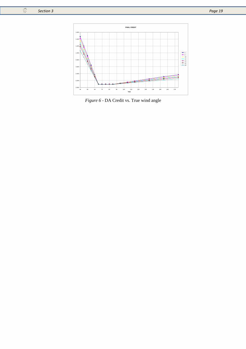
3.5.2 Calculation Procedure
1) Compute the table of polar speeds and GPH without any credit (like all racing boats)
2) Compute DA credits for each true wind speed and wind angle to obtain a matrix with the same row
and columns as the table of speeds.
3) Divide any polar speed of the table by corresponding computed credit and re‐calculate the new
GPH. To compute the DA value (that is printed on certificate only as reference) the ratio between
new and the original GPH is used.
The typical distribution of DA over True wind speed and angle is shown in Figure 6.
Section 3 Page 19
Figure 6 - DA Credit vs. True wind angle
FINAL CREDIT
0.00%
0.20%
0.40%
0.60%
0.80%
1.00%
1.20%
1.40%
1.60%
45 55 65 75 85 95 105 115 125 135 145 155 165 175
TWA
6
8
10
12
14
16
20
Section 5 Page 20
4 Lines Processing Program
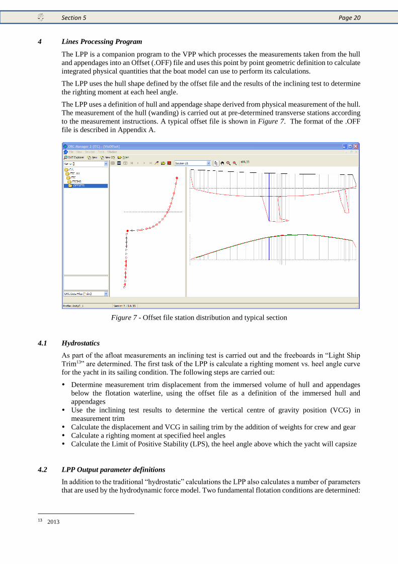
The LPP is a companion program to the VPP which processes the measurements taken from the hull
and appendages into an Offset (.OFF) file and uses this point by point geometric definition to calculate
integrated physical quantities that the boat model can use to perform its calculations.
The LPP uses the hull shape defined by the offset file and the results of the inclining test to determine
the righting moment at each heel angle.
The LPP uses a definition of hull and appendage shape derived from physical measurement of the hull.
The measurement of the hull (wanding) is carried out at pre-determined transverse stations according
to the measurement instructions. A typical offset file is shown in Figure 7. The format of the .OFF
file is described in Appendix A.
Figure 7 - Offset file station distribution and typical section
4.1 Hydrostatics
As part of the afloat measurements an inclining test is carried out and the freeboards in “Light Ship
Trim13” are determined. The first task of the LPP is calculate a righting moment vs. heel angle curve
for the yacht in its sailing condition. The following steps are carried out:
Determine measurement trim displacement from the immersed volume of hull and appendages
below the flotation waterline, using the offset file as a definition of the immersed hull and
appendages
Use the inclining test results to determine the vertical centre of gravity position (VCG) in
measurement trim
Calculate the displacement and VCG in sailing trim by the addition of weights for crew and gear
Calculate a righting moment at specified heel angles
Calculate the Limit of Positive Stability (LPS), the heel angle above which the yacht will capsize
4.2 LPP Output parameter definitions
In addition to the traditional “hydrostatic” calculations the LPP also calculates a number of parameters
that are used by the hydrodynamic force model. Two fundamental flotation conditions are determined:
13 2013
Section 5 Page 21
4.2.1 Measurement Trim
The floatation waterplane is that determined by the measured freeboards with the yacht floating
upright. LSM0 is calculated in this condition using equation [15], and an exponent “nl”= 0.25
4.2.2 Sailing Trim
To achieve sailing trim the default crew weight and gear weight are combined and added to the yacht
0.1 LSM0 aft of the Longitudinal Centre of buoyancy and (0.5 * LSM0 + 0.36) m. above the
measurement trim flotation plane. LSM1 is calculated in this condition using equation [Error!
eference source not found.], and an exponent “nl”= 0.25
4.2.2.1 Crew Weight
The default value for the Crew Weight (kg.) is calculated as follows:
4262.108.25 LSMCW [12]
The owner may accept the default calculated weight, but can declare any crew weight which shall be
recorded in the certificate. The declared crew weight is used to compute increased righting moment
while default crew weight will be used to compute sailing trim displacement.
The longitudinal position of the combined crew longitudinal centre of gravity is calculated from the
formula:
LCBaftLSMcgcrewoflocX __01.0____ [13]
4.2.2.2 Gear Weight
Gear weight is calculated from equation below:
WeightCrewWeightGear _16.0_ [14]
4.2.3 Second Moment Length (LSM)
22
932.3
nl
nl
nl
nl
sdx
xsdx
sdx
sdxxLSM [15]
Where:
s = an element of sectional area attenuated for depth
x = length in the fore and aft direction
nl = Length Exponent
This method of deriving the Effective sailing length from a weighted sectional area curve is a legacy
of the original MHS system. Originally the length calculation took note of the longitudinal volume
distribution of the hull, rather than include directly in the residuary resistance calculation terms that
were calculated from the sectional area curve.
The depth attenuation of sectional areas is performed by multiplying each Z (vertical offset) by
e(-10*Z / LSM0).
The LPP uses the physical shape of the canoe body, as defined by the .OFF offset file, to calculate
immersed lengths at several different waterplane positions.
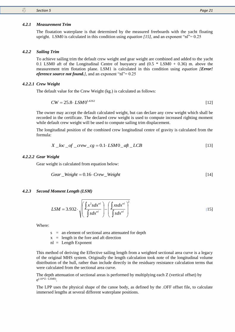
Section 5 Page 22
Figure 8 - Flotation Waterline positions
4.2.4 Appendage stripping
Once the offset file has been acquired and checked, the LPP “strips” off the appendages to leave a
“fair” canoe body. Various hydrostatic characteristics and physical parameters are calculated using the
flotation waterline determined at the in-water measurement. The characteristics of the appendages are
handled separately to determine the parameters that affect their resistance.
4.2.5 Beam Depth Ratio (BTR)
The LPP also computes the effective beam and draft of the yachts canoe body, along with the
maximum effective draft of the keel. The Beam Depth Ratio (BTR) is the effective beam (B) divided
by the effective hull depth (T).
T
BBTR [16]
4.2.5.1 The Effective Beam (B)
The effective beam is calculated based on the transverse second moment of the immersed volume
attenuated with depth for the yacht in Sailing Trim floating upright. This approach “weights” more
heavily elements of hull volume close to the water surface.
dzdxbe
dzdxebB
LSMz
LSMz
010
01033245.3 [17]
where
b = an element of beam;
e = is the Naperian base, 2.7183
z = is depth in the vertical direction
x = length in the fore and aft direction
4.2.5.2 Effective Hull Depth (T)
The Effective Hull Depth is a depth-related quantity for the largest immersed section of the hull. It is
derived from the area of the largest immersed section attenuated with depth for the yacht in Sailing
Trim floating upright (AMS2) divided by B:
Section 5 Page 23
B
AMST
207.2 [18]
4.2.5.3 Maximum Section Areas
Maximum section areas used for the derivation of Effective Hull Depth (T).
AMS1 is the area of the largest immersed section for the yacht in Sailing Trim floating upright.
AMS2 is the area of the largest immersed section attenuated with depth for the yacht in Sailing Trim
floating upright.
Formulae for Maximum Section Areas, (where b is an element of beam; e is the Naperian base, 2.7183;
and z is depth in the vertical direction):
AMS1 = maximum of b dz over length
AMS2 = maximum of b*e(-10*z/LSM0) dz over length
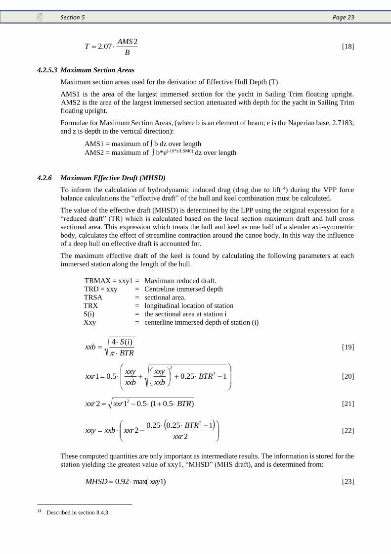
4.2.6 Maximum Effective Draft (MHSD)
To inform the calculation of hydrodynamic induced drag (drag due to lift14) during the VPP force
balance calculations the “effective draft” of the hull and keel combination must be calculated.
The value of the effective draft (MHSD) is determined by the LPP using the original expression for a
“reduced draft” (TR) which is calculated based on the local section maximum draft and hull cross
sectional area. This expression which treats the hull and keel as one half of a slender axi-symmetric
body, calculates the effect of streamline contraction around the canoe body. In this way the influence
of a deep hull on effective draft is accounted for.
The maximum effective draft of the keel is found by calculating the following parameters at each
immersed station along the length of the hull.
TRMAX = xxy1 = Maximum reduced draft.
TRD = xxy = Centreline immersed depth
TRSA = sectional area.
TRX = longitudinal location of station
S(i) = the sectional area at station i
Xxy = centerline immersed depth of station (i)
BTR
iSxxb
)(4 [19]
125.05.01 2
2
BTRxxb
xxy
xxb
xxyxxr [20]
)5.01(5.012 2 BTRxxrxxr [21]
2
125.025.02
2
xxr
BTRxxrxxbxxy [22]
These computed quantities are only important as intermediate results. The information is stored for the
station yielding the greatest value of xxy1, “MHSD” (MHS draft), and is determined from:
)1max(92.0 xxyMHSD [23]
14 Described in section 8.4.3
Section 5 Page 24
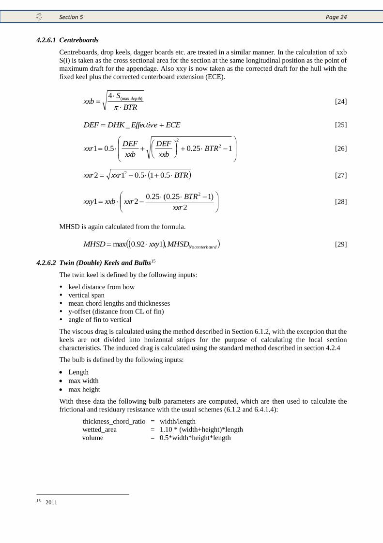
4.2.6.1 Centreboards
Centreboards, drop keels, dagger boards etc. are treated in a similar manner. In the calculation of xxb
S(i) is taken as the cross sectional area for the section at the same longitudinal position as the point of
maximum draft for the appendage. Also xxy is now taken as the corrected draft for the hull with the
fixed keel plus the corrected centerboard extension (ECE).
BTR
Sxxb
depth
)(max4 [24]
ECEEffectiveDHKDEF _ [25]
125.05.01 2
2
BTRxxb
DEF
xxb
DEFxxr [26]
BTRxxrxxr 5.015.012 2 [27]
2
)125.0(25.021
2
xxr
BTRxxrxxbxxy [28]
MHSD is again calculated from the formula.
ardNocenterboMHSDxxyMHSD ,192.0max [29]
4.2.6.2 Twin (Double) Keels and Bulbs15
The twin keel is defined by the following inputs:
keel distance from bow vertical span mean chord lengths and thicknesses y-offset (distance from CL of fin) angle of fin to vertical
The viscous drag is calculated using the method described in Section 6.1.2, with the exception that the
keels are not divided into horizontal stripes for the purpose of calculating the local section
characteristics. The induced drag is calculated using the standard method described in section 4.2.4
The bulb is defined by the following inputs:
Length
max width
max height
With these data the following bulb parameters are computed, which are then used to calculate the
frictional and residuary resistance with the usual schemes (6.1.2 and 6.4.1.4):
thickness_chord_ratio = width/length
wetted_area = 1.10 * (width+height)*length
volume = 0.5*width*height*length
15 2011
Section 5 Page 25
4.2.7 Bulb/Wing Effects
The geometry of the keel tip is influential on the induced drag of the keel fin. These effects may be
both positive and negative,
A ballast bulb with circular (or elliptical) cross section reduces the effect span of the keel fin.
A well designed wing keel extends the effective span of the keel.
The VPP contains an algorithm which detects the type and degree of “bulb” keel or “wing” keel and
modifies the effective span, derived according to section 4.3.4.
4.2.7.1 Definitions
DHK0 geometric overall draft of keel
MAXW max width of keel
TMAXW draft at max width of keel
MAXW and TMAXW are corrected by “10° line test”
FLAGBULB 1 if bulb is detected
FLAGWING 1 if winglets are detected
UPBULBF upper shape factor for bulb
DeltaD effective draft correction due to bulb and/or winglet.
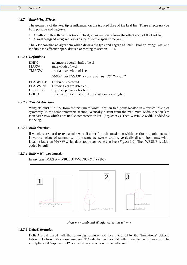
4.2.7.2 Winglet detection
Winglets exist if a line from the maximum width location to a point located in a vertical plane of
symmetry, in the same transverse section, vertically distant from the maximum width location less
than MAXW/4 which does not lie somewhere in keel (Figure 9-1). Then WWING: width is added by
the wing.
4.2.7.3 Bulb detection
If winglets are not detected, a bulb exists if a line from the maximum width location to a point located
in vertical plane of symmetry, in the same transverse section, vertically distant from max width
location less than MAXW which does not lie somewhere in keel (Figure 9-2). Then WBULB is width
added by bulb.
4.2.7.4 Bulb + Winglet detection
In any case: MAXW= WBULB+WWING (Figure 9-3)
Figure 9 - Bulb and Winglet detection scheme
4.2.7.5 DeltaD formulas
DeltaD is calculated with the following formulae and then corrected by the “limitations” defined
below. The formulations are based on CFD calculations for eight bulb or winglet configurations. The
multiplier of 0.5 applied to f2 is an arbitrary reduction of the bulb credit.
Section 5 Page 26
03
025.0
5.0 DHK
MAXWfFlagwing
WBULBWWINGFlagwing
WBULB
DHK
WBULBfUPBULBFFlagbulb
MAXW
TMAXWDHKO
MHSD
DeltaD [30]
Note that:
f2 addresses the bulb effect if there is no winglet
f3 addresses winglet effect if there is no bulb
in the case where bulb and winglet exist the interactions are taken into account by multiplying f2
value by the WBULB/(Flagwing*WWING+WBULB) term
where:
f1(X) = if X<1 1+ k1*X if X>1 1+k1
f2(X) = if X>wbu_T0 k2_0 + k2_1*(X-wbu_T0) if X<=wbu_T0 k2_0 * X / wbu_T0
f3(X) = if X < wwi_T0 k3_0* X / wwi_T0 if X>= wwi_T0 k3_0 + k3_1 * (X-wwi_T0)
k1 0.6 k2_0 -0.06 k2_1 0.19 k3_0 0.05 k3_1 0.02 wbu_T0 0.15 wwi_T0 0.5
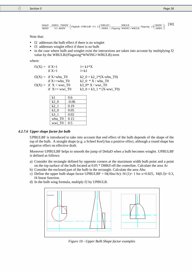
4.2.7.6 Upper shape factor for bulb
UPBULBF is introduced to take into account that end effect of the bulb depends of the shape of the
top of the bulb. A straight shape (e.g. a Scheel Keel) has a positive effect, although a round shape has
negative effect on effective draft.
Moreover UPBULBF helps to smooth the jump of DeltaD when a bulb becomes winglet. UPBULBF
is defined as follows:
a) Consider the rectangle defined by opposite corners at the maximum width bulb point and a point
on the top surface of the bulb located at 0.05 * DHK0 off the centerline. Calculate the area Ar
b) Consider the enclosed part of the bulb in the rectangle. Calculate the area Abu
c) Define the upper bulb shape factor UPBULBF = f4(Abu/Ar): f4 (1)= 1 for x=0.825, f4(0.3)= 0.3,
f4 linear function.
d) In the bulb wing formula, multiply f2 by UPBULB.
Figure 10 - Upper Bulb Shape factor examples
Section 5 Page 27
4.2.7.7 Limitations
DeltaD > - 0.025 * DHK0 (credit bulb limitation)
If the widest point of the bulb or winglet is not enough deep with respect to DHK0 and MAXW, the
bulb or winglet are considered to have no effect:
DeltaD = 0 if TMAXW + 3 * MAXW/2 < DHK0
DeltaD is not affected if TMAXW + MAXW/2 > DHK0
DeltaD varies linearly between those two situations.
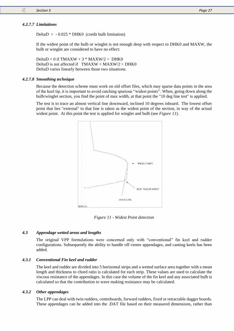
4.2.7.8 Smoothing technique
Because the detection scheme must work on old offset files, which may sparse data points in the area
of the keel tip, it is important to avoid catching spurious “widest points”. When, going down along the
bulb/winglet section, you find the point of max width, at that point the "10 deg line test" is applied.
The test is to trace an almost vertical line downward, inclined 10 degrees inboard. The lowest offset
point that lies "external" to that line is taken as the widest point of the section, in way of the actual
widest point. At this point the test is applied for winglet and bulb (see Figure 11).
Figure 11 - Widest Point detection
4.3 Appendage wetted areas and lengths
The original VPP formulations were concerned only with “conventional” fin keel and rudder
configurations. Subsequently the ability to handle off centre appendages, and canting keels has been
added.
4.3.1 Conventional Fin keel and rudder
The keel and rudder are divided into 5 horizontal strips and a wetted surface area together with a mean
length and thickness to chord ratio is calculated for each strip. These values are used to calculate the
viscous resistance of the appendages. In this case the volume of the fin keel and any associated bulb is
calculated so that the contribution to wave making resistance may be calculated.
4.3.2 Other appendages
The LPP can deal with twin rudders, centreboards, forward rudders, fixed or retractable dagger boards.
These appendages can be added into the .DAT file based on their measured dimensions, rather than
Section 5 Page 28
including them in the wanded .OFF file data. Only the viscous drag of these appendages is calculated,
based on methods described in detail in section 8.1.2. The LPP also calculates any reduction of wetted
surface area that occurs if any dagger board, twin rudder etc. comes above the flotation waterline.
4.4 Righting Moment
4.4.1 Righting Arm Curve
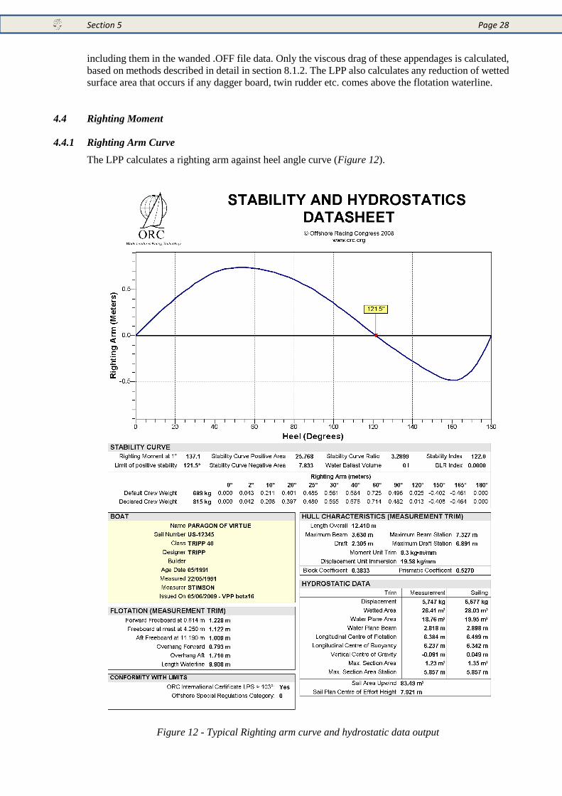
The LPP calculates a righting arm against heel angle curve (Figure 12).
Figure 12 - Typical Righting arm curve and hydrostatic data output
Section 5 Page 29
4.4.2 Hydrodynamic Centre of Pressure
The hydrodynamic vertical center of pressure RM4 is given by:
max43.04 TRM [31]
4.4.3 Crew righting moment
The crew righting moment is based on the declared crew weight or a default crew weight calculated
from 4262.108.25 LSMCW . The assumed individual crew weight is 89 kg and the number of crew
is calculated by dividing the crew weight by this value.
Two less than the total number of crew are distributed along the deck edge of the boat centered about
the assumed centre of gravity position, a single crew member is assumed to occupy a width of 0.53m.
The lever arm of the crew on the rail is the average hull beam over the length of side deck occupied
by the crew. The remaining 2 crew members, the helmsman and main trimmer are assumed to have
transverse centre’s of gravity at 70% of the yachts maximum half beam.
4.4.3.1 LSM greater than 4.9m (16 feet)
For yachts with LSM greater than 4.9 m the crew weight on the rail is 2 less than the total crew, the
remaining 2 are assumed to sit slightly inboard:
)cos(2
27.0 max heelbodywtB
CREWRWCARMmrightingarCrew
[32]
where:
CARM = Crew righting arrm
CREWRW = Crew weight on the rail
Bmax = Hull maximum
bodywt = Average crew body weight.
heel = Heel angle
4.4.3.2 LSM less than 4.9m
For yachts with LSM less than 4.9 m the crew weight is all sat on the rail.
)cos(heelCREWRWCARMmrightingarCrew [33]
4.4.3.3 Crew weight transverse position
Sailing with the upwind sails the crew righting moment is only applied in full once the heel angle
exceeds 6 degrees.
When using the downwind sails (i.e. not a jib), the crew position is set with everyone to leeward up to
a heel=10 deg., then it sinusoidally changes from leeward to neutral from 10 to 14 degrees of heel, and
then sinusoidally moves all the crew to windward from 14 to 18 degrees of heel16.
4.4.4 Dynamic Righting Moment. RMV
RMV is a term intended to account for the difference between the hydrostatic righting moment
calculated by the LPP, and the actual righting moment produced by the hull when moving through the
water. This term was in the VPP from its first implementation17.
SLRAMS
BLSMDSPLRMV
cb
cb 1.21
25.613
10955.5 5
[34]
16 2011 17 The divisor of 3 in the first term was introduced in 2000 to correct an over-prediction of RMV for contemporary hull forms.
Section 5 Page 30
where
DSPL = Displacement
Bcb = Canoe body beam
AMS1cb = Maximum section area of canoe body
SLR = Speed length ratio
4.4.4.1 Dynamic Stability System (DSS)
The DSS is the deployment of an approximately horizontal hydrofoil on the leeward side of the yacht
that generates a vertical force component to augment the yachts righting moment. For 2010 the VPP
will be able to calculate the drag and increased righting moment available from a DSS. The data input
file take in the geometrical data of the foil’s size and position and use a simple algorithm to calculate
the increased righting moment of the foil. The lift force is proportional to the square of the yachts
speed, and the maximum extra righting moment capped at a percentage of the yachts typical sailing
righting moment. Like all features of the IMS VPP this force prediction algorithm is intended to
provide an equitable handicap for yachts fitted with the DSS. It is not a “design and optimization” tool.
4.4.5 Rated Righting Moment
The rated righting moment used in the VPP calculations is the average between the measured and
default RM as follows:
defaultmeasuredrated RMRMRM
3
1
3
2
[35] Default righting moment is calculated as follows18:
IMSLDSPMVOL
Ba
B
HASAa
IMSL
VOLaBTRaaRM default
3343210025.1 [36]
where all the variables are calculated by the VPP using the following coefficient values.
a0 = -0.00410481856369339 (regression coefficient)
a1 = -0.0000399900056441(regression coefficient)
a2 = -0.0001700878169134 (regression coefficient)
a3 = 0.00001918314177143 (regression coefficient)
a4 = 0.00360273975568493 (regression coefficient)
DSPM = displacement in measurement trim
SA = sail area upwind
HA = heeling arm, defined as (CEH main*AREA main + CEH headsail*AREA headsail)
/ SA + HBI + DHKA*0.45, for mizzen (CEH headsail*AREA headsail + CEH
mizzen*AREA mizzen) is added to the numerator
CEH = height of centre of effort
DHKA = Draft of keel and hull adjusted
Default righting moment shall not be taken greater than 1.3*RMmeasured nor smaller than 0.7*RMmeasured.
For movable ballast boats the default righting moment intends to predict the righting moment of the
boat without the effect of movable ballast (water tanks empty, or keel on the center plane), is then
decreased by a factor (1- RM@25_movable/RM@25_tot), where RM@25_movable is the righting
moment due to the contribution of movable ballast at 25 degrees of heel, and RM@25_tot is the total
righting moment at 25 degrees, with keel canted or windward tanks full. For these boats, the max and
min bounds are set to 1.0 x RMmeasured and 0.9 x RMmeasured respectively.
If righting moment is not measured or obtained from another source, the rated righting moment shall
be increased for 3% and shall not be taken less than one giving the Limit of positive stability (LPS) of
103.0 degrees or 90.0 degrees for an ORC Sportboat.
18 1.025 multiplier added 2013
Section 5 Page 31
5 Aerodynamic Forces
The VPP assumes that each individual sail, mainsail, jib, spinnaker, gennaker or code zero can be
characterized by a maximum achievable lift coefficient and a corresponding viscous drag coefficient
that are continuous functions of apparent wind angle. The values of these coefficients are adjusted
depending on the exact sail type and the mast and rigging configuration. The individual coefficients
are then combined into a set of complete sail plan (main and jib, or main and spinnaker) coefficients.
In order to simulate the reduction of heeling force by the crew trimming and changing sails “Flat” and
“Reef” parameters are used.
The flat parameter is used to simulate the reduction of the lift coefficient. It reduces from a value of
1.0, associated with maximum lift, to a minimum value of 0.6 for normally rigged yachts19, i.e. the lift
coefficient reduced by 40%.
The reef parameter simulates the reduction of sail area. When reefing is required to achieve optimum
performance the genoa sail area is first reduced until the genoa reaches it minimum foot length, if
further heeling force reduction is required the mainsail is reefed.
The VPP optimizer is at liberty to de-power the sails by reducing the maximum lift coefficient (Flat)
and reduce sail size (Reef) to achieve best performance at each prescribed True wind angle.
5.1 Methodology
The aerodynamic forces acting on the yacht are resolved into two orthogonal components, lift and
drag. The lift force acts perpendicular to the apparent wind direction and the drag force acts parallel
to it. The force model incorporates 3 sources of drag:
1) The base drag associated with the windage of the hull, spars, rigging and crew;
2) The parasitic drag associated with the skin friction drag of the sails, and the pressure drag associated
with flow separation. The parasitic drag is assumed not to depend on the sail lift force, it does
however vary with the point of sailing;
3) The induced drag, which arises from the three-dimensional nature of the flow around the sails, and
the loss of circulation from the head and foot of the sails. The induced drag is assumed to vary as
the square of the lift coefficient. A two-dimensional lift dependant drag term is also added to the
basic induced drag.
Analysis of the rig begins by ascribing the appropriate coefficient set to the main, jib and offwind sails.
The frontal and side areas associated with the mast, hull and rigging are also calculated. Each area has
an associated vertical centre of force which represents the height at which all the aerodynamic loads
could be concentrated to produce the same overall rolling moment. Because the presence of a wind
gradient implies that the wind velocity is a function of height, the vertical heights of the centres of
force are used when evaluating the dynamic pressure acting on any aerodynamic surface.
5.1.1 Individual Sail Areas and 2-Dimensional Aerodynamic Force Coefficients
The fundamental components of the aerodynamic model are the individual sails, characterised by the
following parameters, which are shown diagrammatically in Figure 13:
Sail area
Centre of effort height above the sail’s datum
ClX and CdP versus AW envelope. (Maximum lift coefficient and parasitic (viscous) drag coefficient
versus apparent wind angle).
19 This minimum flat value of 0.6 is based on the lift force reduction that has been observed in wind tunnel tests.
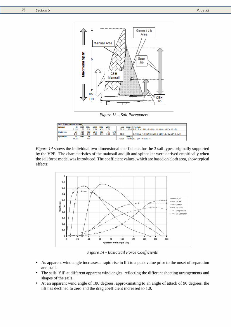
Section 5 Page 32
Figure 13 – Sail Parematers
Figure 14 shows the individual two-dimensional coefficients for the 3 sail types originally supported
by the VPP. The characteristics of the mainsail and jib and spinnaker were derived empirically when
the sail force model was introduced. The coefficient values, which are based on cloth area, show typical
effects:
Figure 14 - Basic Sail Force Coefficients
As apparent wind angle increases a rapid rise in lift to a peak value prior to the onset of separation
and stall.
The sails ‘fill’ at different apparent wind angles, reflecting the different sheeting arrangements and
shapes of the sails.
At an apparent wind angle of 180 degrees, approximating to an angle of attack of 90 degrees, the
lift has declined to zero and the drag coefficient increased to 1.0.
0
0.2
0.4
0.6
0.8
1
1.2
1.4
1.6
1.8
2
0 20 40 60 80 100 120 140 160 180
Apparent Wind Angle (deg.)
Co
eff
icie
nt
Cl Jib
Cd Jib
Cl Main
Cd Main
Cl Spinnaker
Cd Spinnaker
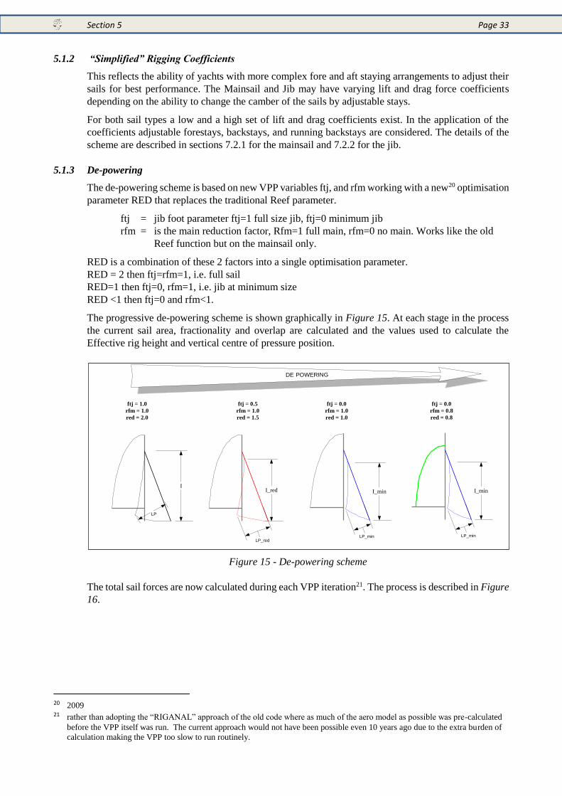
Section 5 Page 33
5.1.2 “Simplified” Rigging Coefficients
This reflects the ability of yachts with more complex fore and aft staying arrangements to adjust their
sails for best performance. The Mainsail and Jib may have varying lift and drag force coefficients
depending on the ability to change the camber of the sails by adjustable stays.
For both sail types a low and a high set of lift and drag coefficients exist. In the application of the
coefficients adjustable forestays, backstays, and running backstays are considered. The details of the
scheme are described in sections 7.2.1 for the mainsail and 7.2.2 for the jib.
5.1.3 De-powering
The de-powering scheme is based on new VPP variables ftj, and rfm working with a new20 optimisation
parameter RED that replaces the traditional Reef parameter.
ftj = jib foot parameter ftj=1 full size jib, ftj=0 minimum jib
rfm = is the main reduction factor, Rfm=1 full main, rfm=0 no main. Works like the old
Reef function but on the mainsail only.
RED is a combination of these 2 factors into a single optimisation parameter.
RED = 2 then ftj=rfm=1, i.e. full sail
RED=1 then ftj=0, rfm=1, i.e. jib at minimum size
RED <1 then ftj=0 and rfm<1.
The progressive de-powering scheme is shown graphically in Figure 15. At each stage in the process
the current sail area, fractionality and overlap are calculated and the values used to calculate the
Effective rig height and vertical centre of pressure position.
Figure 15 - De-powering scheme
The total sail forces are now calculated during each VPP iteration21. The process is described in Figure
16.
20 2009 21 rather than adopting the “RIGANAL” approach of the old code where as much of the aero model as possible was pre-calculated
before the VPP itself was run. The current approach would not have been possible even 10 years ago due to the extra burden of
calculation making the VPP too slow to run routinely.
I
LP
I_min
LP_min
HE_red
I_red
LP_red
OLAP_red
FRAC_red
OLAP_red, FRAC_red, HE_red
DE POWERING
FRAC_red
OLAP, FRAC, HEHE_red
OLAP_red
OLAP_red
FRAC_redFRAC_red
CE_red
OLAP_red
CE_red
ftj = 1.0
rfm = 1.0
red = 2.0
OLAP, FRAC, HE
OLAP_red, FRAC_red, HE_red
OLAP_red
FRAC_red
OLAP_min, FRAC_min, HE_red
HE_red
OLAP_red
FRAC_red
OLAP_min, FRAC_min, HE_red
CE_red
ftj = 0.5
rfm = 1.0
red = 1.5
ftj = 0.0
rfm = 1.0
red = 1.0
ftj = 0.0
rfm = 0.8
red = 0.8
I_min
LP_min
OLAP_red
FRAC_red
OLAP_min, FRAC_red, HE_red
OLAP_red
FRAC_red
OLAP_min, FRAC_red, HE_red
HE_red
CE_red
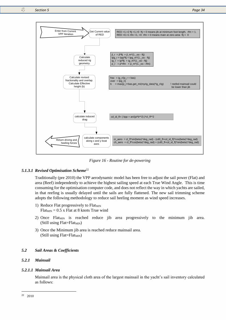
Section 5 Page 34
Figure 16 - Routine for de-powering
5.1.3.1 Revised Optimisation Scheme22
Traditionally (pre 2010) the VPP aerodynamic model has been free to adjust the sail power (Flat) and
area (Reef) independently to achieve the highest sailing speed at each True Wind Angle. This is time
consuming for the optimisation computer code, and does not reflect the way in which yachts are sailed,
in that reefing is usually delayed until the sails are fully flattened. The new sail trimming scheme
adopts the following methodology to reduce sail heeling moment as wind speed increases.
1) Reduce Flat progressively to FlatMIN
FlatMIN = 0.5 x Flat at 8 knots True wind
2) Once FlatMIN is reached reduce jib area progressively to the minimum jib area.
(Still using Flat=FlatMIN)
3) Once the Minimum jib area is reached reduce mainsail area.
(Still using Flat=FlatMIN)
5.2 Sail Areas & Coefficients
5.2.1 Mainsail
5.2.1.1 Mainsail Area
Mainsail area is the physical cloth area of the largest mainsail in the yacht’s sail inventory calculated
as follows:
22 2010
Get Current value
of RED
Calculate
reduced rig
geometry.
Calculate revised
fractionality and overlap.
Calculate Effective
height (b)
calculate induced
drag
calculate components
along x and y boat
axes
Enter from Current VPP Iteration
Return driving and
heeling forces
jl_r = jl*ftj + jl_m*(1._oo - ftj)
lpg_r = lpg*ftj + lpg_m*(1._oo - ftj)
ig_r = ig*ftj + ig_m*(1._oo - ftj)
p_r = p*rfm + p_m*(1._oo - rfm)
frac = ig_r/(p_r + bas)
over = lpg_r/j
b = max(p_r+bas,get_mi(myrig_data)*ig_r/ig) ! reefed mainsail could
be lower than jib
RED >1,<2 ftj <1,>0 ftj = 0 means jib at minimum foot length, rfm = 1.
RED >0,<1 rfm <1, >0 rfm = 0 means main at zero area ftj = 0
cd_id_fl= ( kpp + an/(pi*b**2) )*cl_fl**2
cr_aero = cl_fl*sin(beta1*deg_rad) - (cd0_fl+cd_id_fl)*cos(beta1*deg_rad)
ch_aero = cl_fl*cos(beta1*deg_rad) + (cd0_fl+cd_id_fl)*sin(beta1*deg_rad)
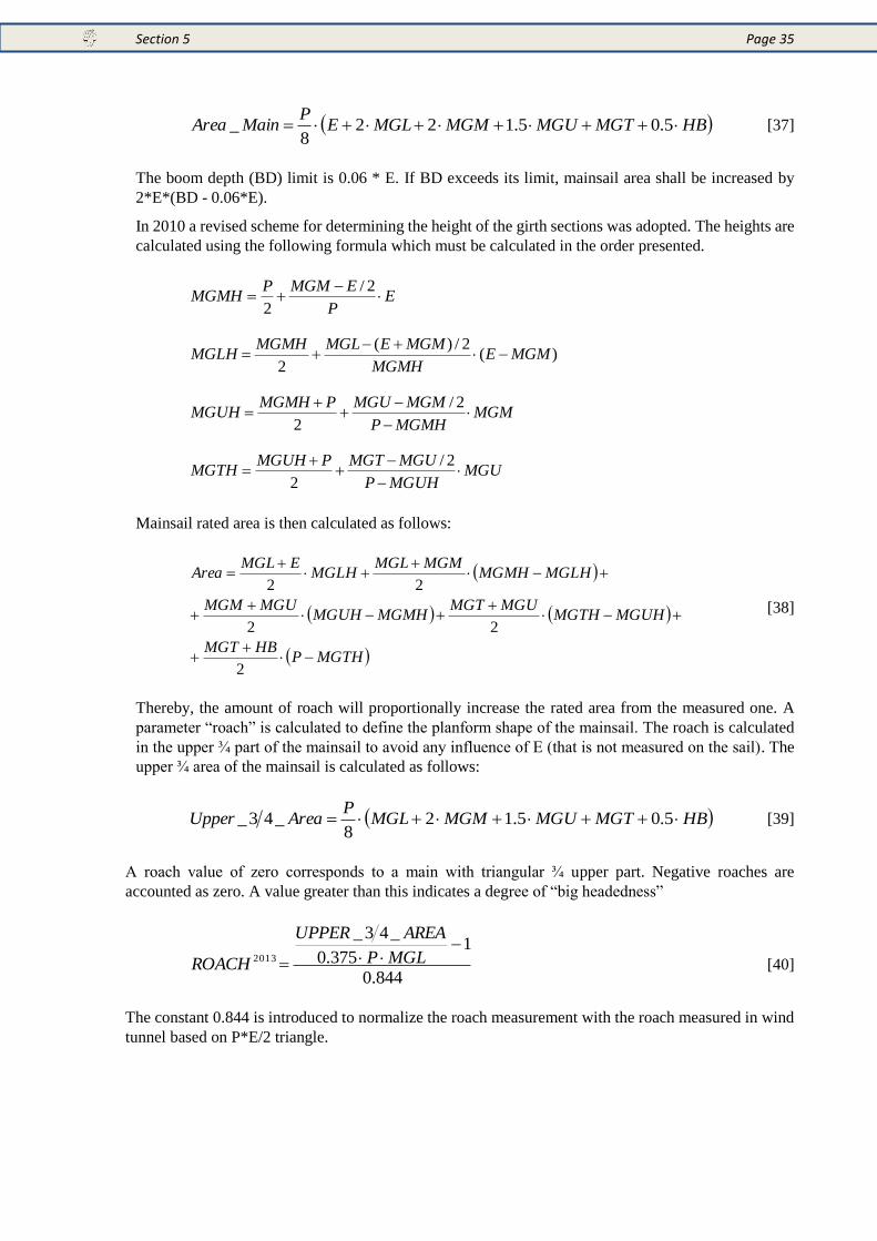
Section 5 Page 35
HBMGTMGUMGMMGLEP
MainArea 5.05.1228
_ [37]
The boom depth (BD) limit is 0.06 * E. If BD exceeds its limit, mainsail area shall be increased by
2*E*(BD - 0.06*E).
In 2010 a revised scheme for determining the height of the girth sections was adopted. The heights are
calculated using the following formula which must be calculated in the order presented.
EP
EMGMPMGMH
2/
2
)(2/)(
2MGME
MGMH
MGMEMGLMGMHMGLH
MGMMGMHP
MGMMGUPMGMHMGUH
2/
2
MGUMGUHP
MGUMGTPMGUHMGTH
2/
2
Mainsail rated area is then calculated as follows:
MGTHPHBMGT
MGUHMGTHMGUMGT
MGMHMGUHMGUMGM
MGLHMGMHMGMMGL
MGLHEMGL
Area
2
22
22
[38]
Thereby, the amount of roach will proportionally increase the rated area from the measured one. A
parameter “roach” is calculated to define the planform shape of the mainsail. The roach is calculated
in the upper ¾ part of the mainsail to avoid any influence of E (that is not measured on the sail). The
upper ¾ area of the mainsail is calculated as follows:
HBMGTMGUMGMMGLP
AreaUpper 5.05.128
_43_ [39]
A roach value of zero corresponds to a main with triangular ¾ upper part. Negative roaches are
accounted as zero. A value greater than this indicates a degree of “big headedness”
844.0
1375.0
_43_
2013
MGLP
AREAUPPER
ROACH [40]
The constant 0.844 is introduced to normalize the roach measurement with the roach measured in wind
tunnel based on P*E/2 triangle.
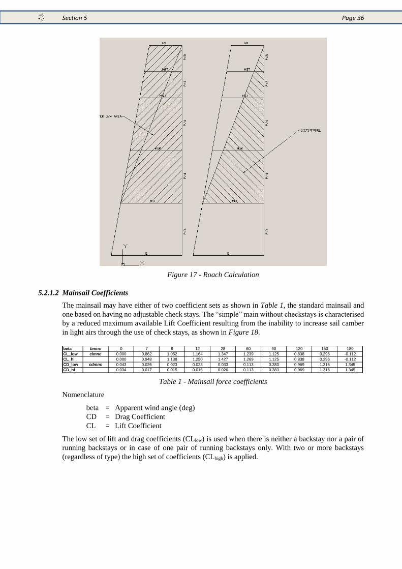
Section 5 Page 36
Figure 17 - Roach Calculation
5.2.1.2 Mainsail Coefficients
The mainsail may have either of two coefficient sets as shown in Table 1, the standard mainsail and
one based on having no adjustable check stays. The “simple” main without checkstays is characterised
by a reduced maximum available Lift Coefficient resulting from the inability to increase sail camber
in light airs through the use of check stays, as shown in Figure 18.
Table 1 - Mainsail force coefficients
Nomenclature
beta = Apparent wind angle (deg)
CD = Drag Coefficient
CL = Lift Coefficient
The low set of lift and drag coefficients (CLlow) is used when there is neither a backstay nor a pair of
running backstays or in case of one pair of running backstays only. With two or more backstays
(regardless of type) the high set of coefficients (CLhigh) is applied.
beta bmnc 0 7 9 12 28 60 90 120 150 180
CL_low clmnc 0.000 0.862 1.052 1.164 1.347 1.239 1.125 0.838 0.296 -0.112
CL_hi 0.000 0.948 1.138 1.250 1.427 1.269 1.125 0.838 0.296 -0.112
CD_low cdmnc 0.043 0.026 0.023 0.023 0.033 0.113 0.383 0.969 1.316 1.345
CD_hi 0.034 0.017 0.015 0.015 0.026 0.113 0.383 0.969 1.316 1.345
dCL dclm04 0.000 0.086 0.086 0.086 0.080 0.030 0.000 0.000 0.000 0.000
dCD dcdm04 0.009 0.009 0.009 0.009 0.007 0.000 0.000 0.000 0.000 0.000
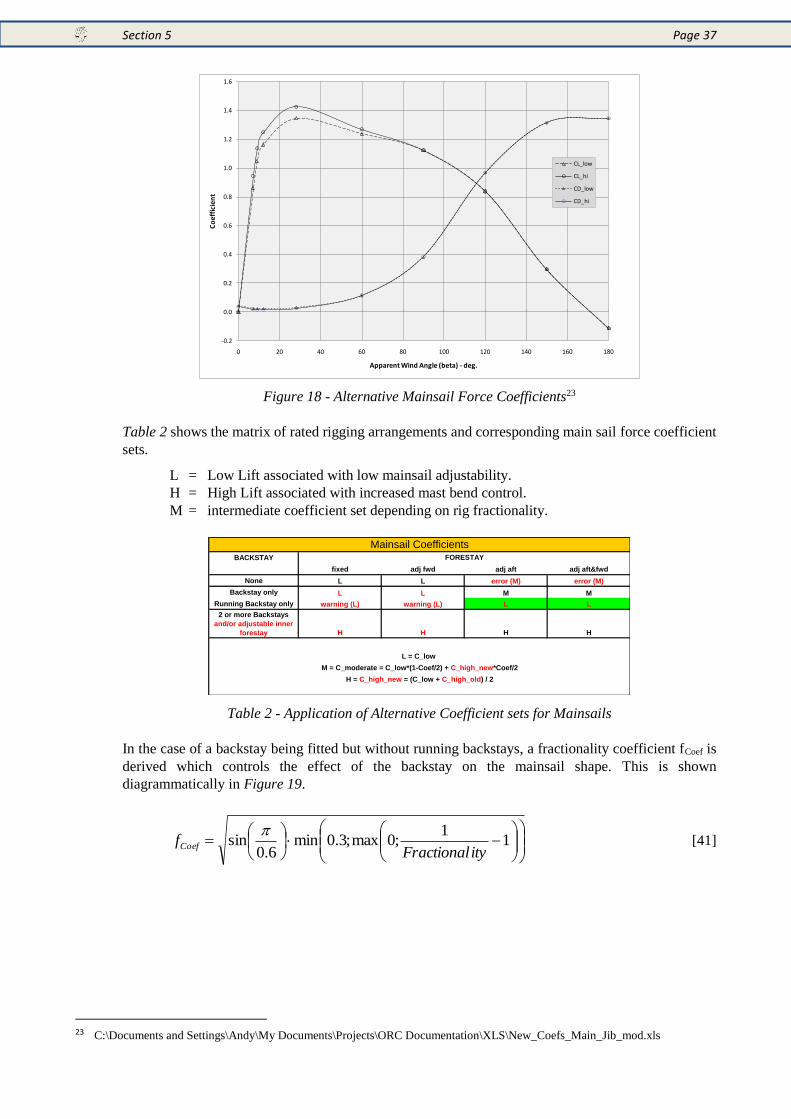
Section 5 Page 37
Figure 18 - Alternative Mainsail Force Coefficients23
Table 2 shows the matrix of rated rigging arrangements and corresponding main sail force coefficient
sets.
L = Low Lift associated with low mainsail adjustability.
H = High Lift associated with increased mast bend control.
M = intermediate coefficient set depending on rig fractionality.
Table 2 - Application of Alternative Coefficient sets for Mainsails
In the case of a backstay being fitted but without running backstays, a fractionality coefficient fCoef is
derived which controls the effect of the backstay on the mainsail shape. This is shown
diagrammatically in Figure 19.
1
1;0max;3.0min
6.0sin
ityFractionalfCoef
[41]
23 C:\Documents and Settings\Andy\My Documents\Projects\ORC Documentation\XLS\New_Coefs_Main_Jib_mod.xls
-0.2
0.0
0.2
0.4
0.6
0.8
1.0
1.2
1.4
1.6
0 20 40 60 80 100 120 140 160 180
Co
effi
cien
t
Apparent Wind Angle (beta) - deg.
CL_low
CL_hi
CD_low
CD_hi
BACKSTAY
fixed adj fwd adj aft adj aft&fwd
None L L error (M) error (M)
Backstay only L L M M
Running Backstay only warning (L) warning (L) L L
2 or more Backstays
and/or adjustable inner
forestay H H H H
Mainsail CoefficientsFORESTAY
L = C_low
M = C_moderate = C_low*(1-Coef/2) + C_high_new*Coef/2
H = C_high_new = (C_low + C_high_old) / 2
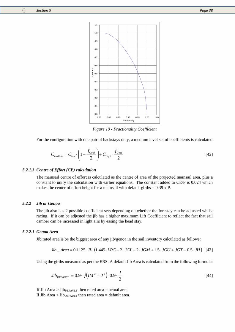
Section 5 Page 38
Figure 19 - Fractionality Coefficient
For the configuration with one pair of backstays only, a medium level set of coefficients is calculated
22
1Coef
high
Coef
lowmedium
fC
fCC
[42]
5.2.1.3 Centre of Effort (CE) calculation
The mainsail centre of effort is calculated as the centre of area of the projected mainsail area, plus a
constant to unify the calculation with earlier equations. The constant added to CE/P is 0.024 which
makes the center of effort height for a mainsail with default girths = 0.39 x P.
5.2.2 Jib or Genoa
The jib also has 2 possible coefficient sets depending on whether the forestay can be adjusted whilst
racing. If it can be adjusted the jib has a higher maximum Lift Coefficient to reflect the fact that sail
camber can be increased in light airs by easing the head stay.
5.2.2.1 Genoa Area
Jib rated area is be the biggest area of any jib/genoa in the sail inventory calculated as follows:
JHJGTJGUJGMJGLLPGJLAreaJib 5.05.122445.11125.0_ [43]
Using the girths measured as per the ERS. A default Jib Area is calculated from the following formula:
2
9.09.0 22 JJIMJibDEFAULT [44]
If Jib Area > JibDEFAULT then rated area = actual area.
If Jib Area < JibDEFAULT then rated area = default area.
0.0
0.1
0.2
0.3
0.4
0.5
0.6
0.7
0.8
0.9
1.0
1.1
0.75 0.80 0.85 0.90 0.95 1.00 1.05
Co
ef C
C
Fractionality
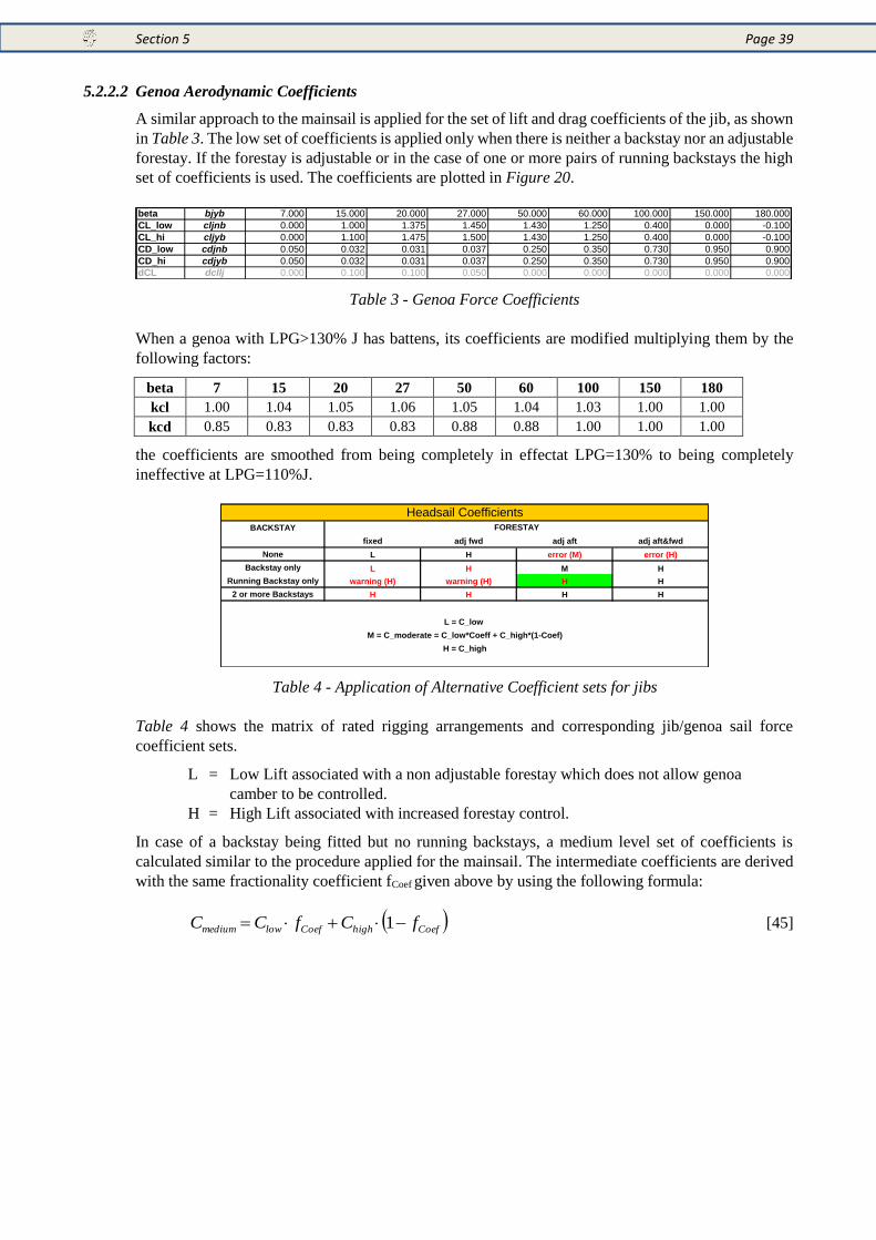
Section 5 Page 39
5.2.2.2 Genoa Aerodynamic Coefficients
A similar approach to the mainsail is applied for the set of lift and drag coefficients of the jib, as shown
in Table 3. The low set of coefficients is applied only when there is neither a backstay nor an adjustable
forestay. If the forestay is adjustable or in the case of one or more pairs of running backstays the high
set of coefficients is used. The coefficients are plotted in Figure 20.
Table 3 - Genoa Force Coefficients
When a genoa with LPG>130% J has battens, its coefficients are modified multiplying them by the
following factors:
beta 7 15 20 27 50 60 100 150 180
kcl 1.00 1.04 1.05 1.06 1.05 1.04 1.03 1.00 1.00
kcd 0.85 0.83 0.83 0.83 0.88 0.88 1.00 1.00 1.00
the coefficients are smoothed from being completely in effectat LPG=130% to being completely
ineffective at LPG=110%J.
Table 4 - Application of Alternative Coefficient sets for jibs
Table 4 shows the matrix of rated rigging arrangements and corresponding jib/genoa sail force
coefficient sets.
L = Low Lift associated with a non adjustable forestay which does not allow genoa
camber to be controlled.
H = High Lift associated with increased forestay control.
In case of a backstay being fitted but no running backstays, a medium level set of coefficients is
calculated similar to the procedure applied for the mainsail. The intermediate coefficients are derived
with the same fractionality coefficient fCoef given above by using the following formula:
CoefhighCoeflowmedium fCfCC 1 [45]
beta bjyb 7.000 15.000 20.000 27.000 50.000 60.000 100.000 150.000 180.000
CL_low cljnb 0.000 1.000 1.375 1.450 1.430 1.250 0.400 0.000 -0.100
CL_hi cljyb 0.000 1.100 1.475 1.500 1.430 1.250 0.400 0.000 -0.100
CD_low cdjnb 0.050 0.032 0.031 0.037 0.250 0.350 0.730 0.950 0.900
CD_hi cdjyb 0.050 0.032 0.031 0.037 0.250 0.350 0.730 0.950 0.900
dCL dcllj 0.000 0.100 0.100 0.050 0.000 0.000 0.000 0.000 0.000
BACKSTAY
fixed adj fwd adj aft adj aft&fwd
None L H error (M) error (H)
Backstay only L H M H
Running Backstay only warning (H) warning (H) H H
2 or more Backstays H H H H
M = C_moderate = C_low*Coeff + C_high*(1-Coef)
H = C_high
Headsail CoefficientsFORESTAY
L = C_low
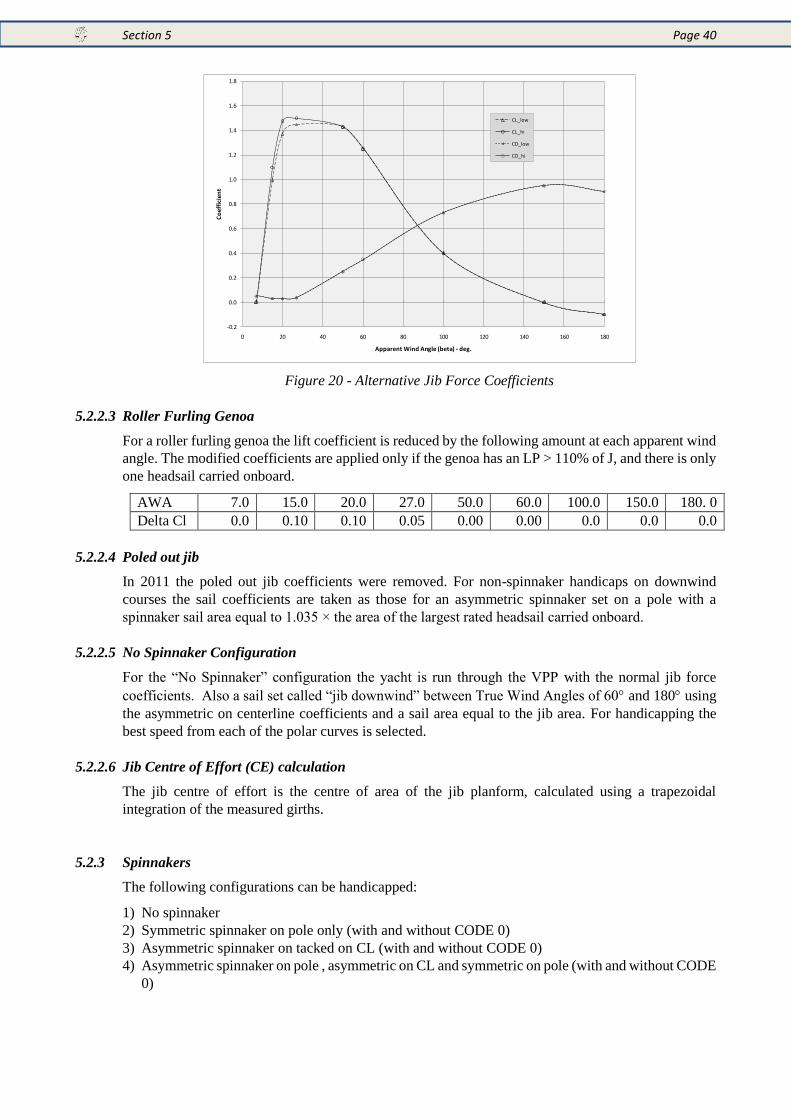
Section 5 Page 40
Figure 20 - Alternative Jib Force Coefficients
5.2.2.3 Roller Furling Genoa
For a roller furling genoa the lift coefficient is reduced by the following amount at each apparent wind
angle. The modified coefficients are applied only if the genoa has an LP > 110% of J, and there is only
one headsail carried onboard.
AWA 7.0 15.0 20.0 27.0 50.0 60.0 100.0 150.0 180. 0
Delta Cl 0.0 0.10 0.10 0.05 0.00 0.00 0.0 0.0 0.0
5.2.2.4 Poled out jib
In 2011 the poled out jib coefficients were removed. For non-spinnaker handicaps on downwind
courses the sail coefficients are taken as those for an asymmetric spinnaker set on a pole with a
spinnaker sail area equal to 1.035 × the area of the largest rated headsail carried onboard.
5.2.2.5 No Spinnaker Configuration
For the “No Spinnaker” configuration the yacht is run through the VPP with the normal jib force
coefficients. Also a sail set called “jib downwind” between True Wind Angles of 60 and 180 using
the asymmetric on centerline coefficients and a sail area equal to the jib area. For handicapping the
best speed from each of the polar curves is selected.
5.2.2.6 Jib Centre of Effort (CE) calculation
The jib centre of effort is the centre of area of the jib planform, calculated using a trapezoidal
integration of the measured girths.
5.2.3 Spinnakers
The following configurations can be handicapped:
1) No spinnaker
2) Symmetric spinnaker on pole only (with and without CODE 0)
3) Asymmetric spinnaker on tacked on CL (with and without CODE 0)
4) Asymmetric spinnaker on pole , asymmetric on CL and symmetric on pole (with and without CODE
0)
-0.2
0.0
0.2
0.4
0.6
0.8
1.0
1.2
1.4
1.6
1.8
0 20 40 60 80 100 120 140 160 180
Co
eff
icie
nt
Apparent Wind Angle (beta) - deg.
CL_low
CL_hi
CD_low
CD_hi
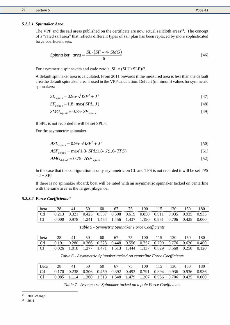
Section 5 Page 41
5.2.3.1 Spinnaker Area
The VPP and the sail areas published on the certificate are now actual sailcloth areas24. The concept
of a “rated sail area” that reflects different types of sail plan has been replaced by more sophisticated
force coefficient sets.
6
4ker_
SMGSFSLareaSpinna
[46]
For asymmetric spinnakers and code zero’s, SL = (SLU+SLE)/2.
A default spinnaker area is calculated. From 2011 onwards if the measured area is less than the default
area the default spinnaker area is used in the VPP calculation. Default (minimum) values for symmetric
spinnakers:
2295.0 JISPSLdefualt [47]
),max(8.1 JSPLSFdefault [48]
defaultdefault SFSMG 75.0 [49]
If SPL is not recorded it will be set SPL=J
For the asymmetric spinnaker:
2295.0 JISPASLdefault [50]
)6.1;8.1;8.1max( TPSJSPLASFdefault [51]
defaultdefault ASFAMG 75.0 [52]
In the case that the configuration is only asymmetric on CL and TPS is not recorded it will be set TPS
= J + SFJ
If there is no spinnaker aboard; boat will be rated with an asymmetric spinnaker tacked on centerline
with the same area as the largest jib/genoa.
5.2.3.2 Force Coefficients25
beta 28 41 50 60 67 75 100 115 130 150 180
Cd 0.213 0.321 0.425 0.587 0.598 0.619 0.850 0.911 0.935 0.935 0.935
Cl 0.000 0.978 1.241 1.454 1.456 1.437 1.190 0.951 0.706 0.425 0.000
Table 5 - Symmetric Spinnaker Force Coefficients
beta 28 41 50 60 67 75 100 115 130 150 180
Cd 0.191 0.280 0.366 0.523 0.448 0.556 0.757 0.790 0.776 0.620 0.400
Cl 0.026 1.018 1.277 1.471 1.513 1.444 1.137 0.829 0.560 0.250 0.120
Table 6 - Asymmetric Spinnaker tacked on centreline Force Coefficients
Beta 28 41 50 60 67 75 100 115 130 150 180
Cd 0.170 0.238 0.306 0.459 0.392 0.493 0.791 0.894 0.936 0.936 0.936
Cl 0.085 1.114 1.360 1.513 1.548 1.479 1.207 0.956 0.706 0.425 0.000
Table 7 - Asymmetric Spinnaker tacked on a pole Force Coefficients
24 2008 change 25 2011
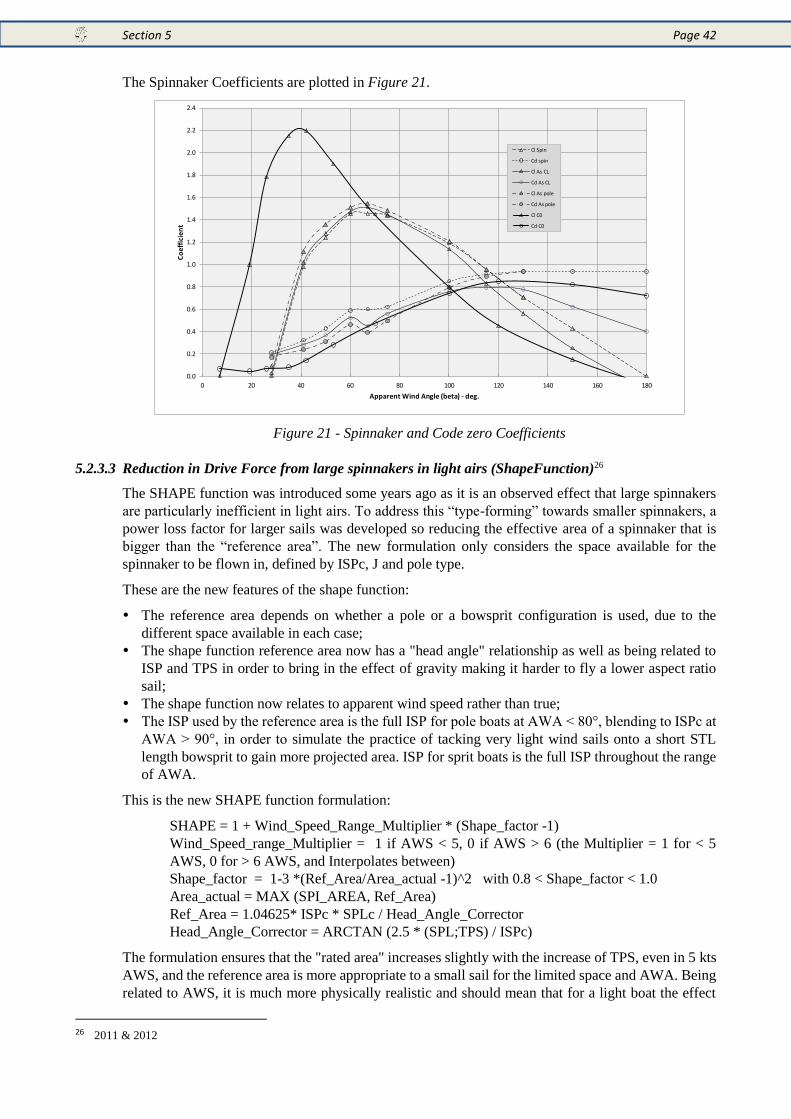
Section 5 Page 42
The Spinnaker Coefficients are plotted in Figure 21.
Figure 21 - Spinnaker and Code zero Coefficients
5.2.3.3 Reduction in Drive Force from large spinnakers in light airs (ShapeFunction)26
The SHAPE function was introduced some years ago as it is an observed effect that large spinnakers
are particularly inefficient in light airs. To address this “type-forming” towards smaller spinnakers, a
power loss factor for larger sails was developed so reducing the effective area of a spinnaker that is
bigger than the “reference area”. The new formulation only considers the space available for the
spinnaker to be flown in, defined by ISPc, J and pole type.
These are the new features of the shape function:
The reference area depends on whether a pole or a bowsprit configuration is used, due to the
different space available in each case; The shape function reference area now has a "head angle" relationship as well as being related to
ISP and TPS in order to bring in the effect of gravity making it harder to fly a lower aspect ratio
sail; The shape function now relates to apparent wind speed rather than true; The ISP used by the reference area is the full ISP for pole boats at AWA < 80°, blending to ISPc at
AWA > 90°, in order to simulate the practice of tacking very light wind sails onto a short STL
length bowsprit to gain more projected area. ISP for sprit boats is the full ISP throughout the range
of AWA.
This is the new SHAPE function formulation:
SHAPE = 1 + Wind_Speed_Range_Multiplier * (Shape_factor -1)
Wind_Speed_range_Multiplier = 1 if AWS < 5, 0 if AWS > 6 (the Multiplier = 1 for < 5
AWS, 0 for > 6 AWS, and Interpolates between)
Shape_factor = 1-3 *(Ref_Area/Area_actual -1)^2 with 0.8 < Shape_factor < 1.0
Area_actual = MAX (SPI_AREA, Ref_Area)
Ref_Area = 1.04625* ISPc * SPLc / Head_Angle_Corrector
Head_Angle_Corrector = ARCTAN (2.5 * (SPL;TPS) / ISPc)
The formulation ensures that the "rated area" increases slightly with the increase of TPS, even in 5 kts
AWS, and the reference area is more appropriate to a small sail for the limited space and AWA. Being
related to AWS, it is much more physically realistic and should mean that for a light boat the effect
26 2011 & 2012
0.0
0.2
0.4
0.6
0.8
1.0
1.2
1.4
1.6
1.8
2.0
2.2
2.4
0 20 40 60 80 100 120 140 160 180
Co
effi
cien
t
Apparent Wind Angle (beta) - deg.
Cl Spin
Cd spin
Cl As CL
Cd As CL
Cl As pole
Cd As pole
Cl C0
Cd C0
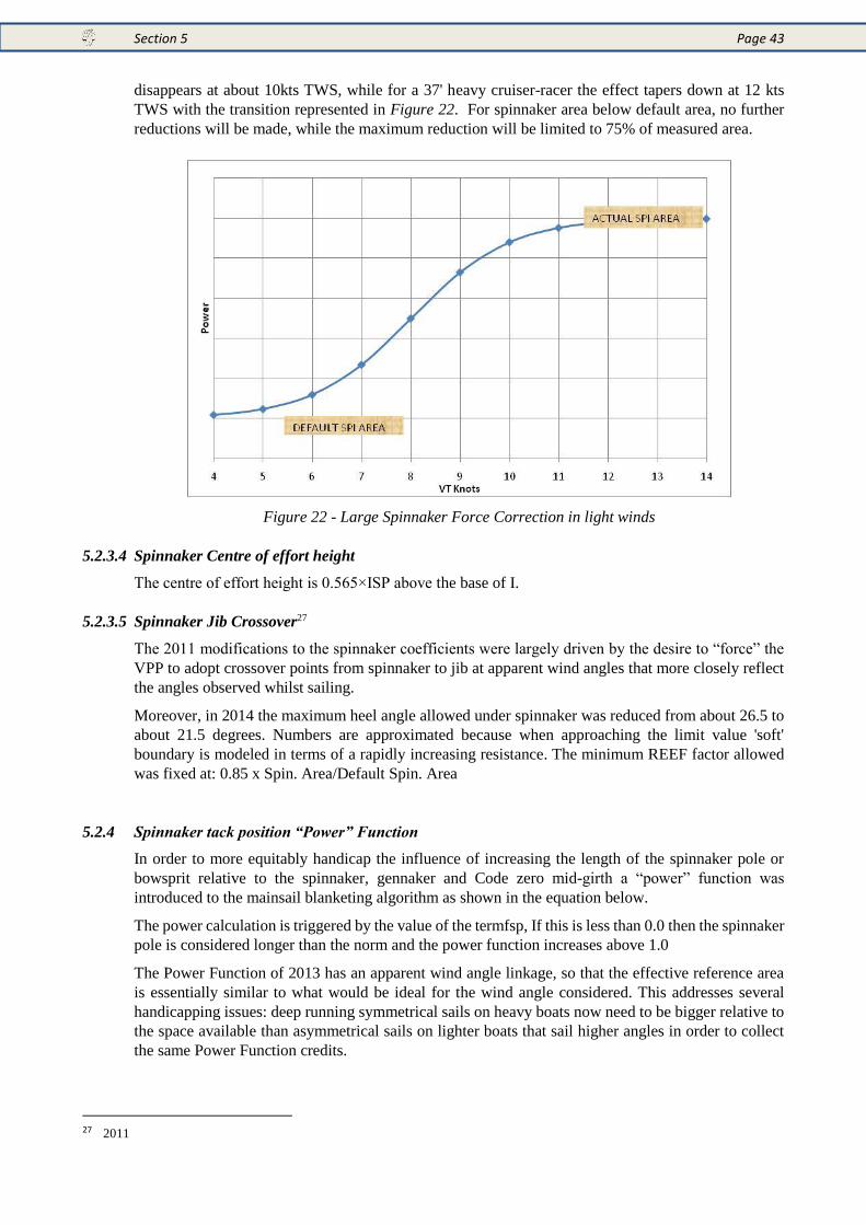
Section 5 Page 43
disappears at about 10kts TWS, while for a 37' heavy cruiser-racer the effect tapers down at 12 kts
TWS with the transition represented in Figure 22. For spinnaker area below default area, no further
reductions will be made, while the maximum reduction will be limited to 75% of measured area.
Figure 22 - Large Spinnaker Force Correction in light winds
5.2.3.4 Spinnaker Centre of effort height
The centre of effort height is 0.565×ISP above the base of I.
5.2.3.5 Spinnaker Jib Crossover27
The 2011 modifications to the spinnaker coefficients were largely driven by the desire to “force” the
VPP to adopt crossover points from spinnaker to jib at apparent wind angles that more closely reflect
the angles observed whilst sailing.
Moreover, in 2014 the maximum heel angle allowed under spinnaker was reduced from about 26.5 to
about 21.5 degrees. Numbers are approximated because when approaching the limit value 'soft'
boundary is modeled in terms of a rapidly increasing resistance. The minimum REEF factor allowed
was fixed at: 0.85 x Spin. Area/Default Spin. Area
5.2.4 Spinnaker tack position “Power” Function
In order to more equitably handicap the influence of increasing the length of the spinnaker pole or
bowsprit relative to the spinnaker, gennaker and Code zero mid-girth a “power” function was
introduced to the mainsail blanketing algorithm as shown in the equation below.
The power calculation is triggered by the value of the termfsp, If this is less than 0.0 then the spinnaker
pole is considered longer than the norm and the power function increases above 1.0
The Power Function of 2013 has an apparent wind angle linkage, so that the effective reference area
is essentially similar to what would be ideal for the wind angle considered. This addresses several
handicapping issues: deep running symmetrical sails on heavy boats now need to be bigger relative to
the space available than asymmetrical sails on lighter boats that sail higher angles in order to collect
the same Power Function credits.
27 2011
Section 5 Page 44
First, bowsprits are considered shorter than poles (a reduction factor of 0.9 is applied to TPS) while a
correction of height available is taken into account for poles as 0.16*LSM1, considering that poles are
set higher than the bowsprit.
The power formulation28 is:
Power = 0.92 + (ABS (fsp)) ^1.5, but not to exceed 1.2
Fsp= min((1-1.488*SPLc/(SPI_AREA/(ISPc*AWAfact))-0.17 , 0 )
SPLc= SPL or 0.9*TPS
ISPc= ISP( for sprit) or ISP-0.16*LSM1 (for poles)
AWAfact = 0.5196*AWA^0.1274 if AWA>28°, 0.794 if AWA<28°
CE height = 0.517*ISPc+0.16*LSM1 for poles or 0.517*ISPc for sprit,
In 2014 power function was fine tuned: the upper last 5% of mast height is for free in ISP for the sake
of power function calculation: ISPc = min(ISPc,0.95*(P+BAS)).
The fsp formulation includes ISP and TPS, so in effect it has dimensions of an area. The AWA factor
is a modification on this area to consider a boat type that needs to sail at 175 degrees and can fill the
available space with a larger spinnaker more effectively than a boat that needs to sail at 100 degrees
that would not benefit from such a large spinnaker. So if a typical A1 area is set at a typical A1 angle,
it should reach a similar power factor to a typical S4 or A4 area set at their typically-wider angles. The
“Power” function does not credit poles or bowsprits shorter than the norm, and the maximum power
increment is 20% above the base level.
In order to calculate the force from the spinnaker/gennaker the sail area is multiplied by the Power
function.
5.2.5 Headsails set flying
Since 2014 the former code0 has been renamed as headsail set flying, and some modifications have
been introduced to the rules, affecting the way its area is computed, and its performances. The flying
headsail area is now measured similarly to the jib and genoa (which are headsails too, but not set
flying).
Regarding the aerodynamic coefficients, it has been acknowledged that there is a big variety of flying
headsails: they could be conceived for close reaching and upwind sailing similarly to a genoa or jib,
or they can be designed to give their maximum performance at wider angles. With the aim of catching
this variety two characteristics of the sail are taken into account: the presence of battens and that of a
tight luff . A flying headsail designed for upwind sailing will normally have a tightluff and battens,
while a sail for wider angles will have a loose luff, and will not be able to perform as well upwind.
5.2.5.1 Area calculation and legacy conversion
The area formula for flying headsail is the same as for jibs/genoa (now all called headsails):
Area = 0.1125*JL*(1.4444444*LPG+2*JGL+2*JGM+1.5*JGU+JGT+0.5*JH)
The old code0s area was based on spinnaker formula:
Area_old=0.5*(SLU+SLE)*(4*AMG+ASF)/6
During the transition 2013-2014 for legacy code0s a conversion formula that preserves
JGM/LPG=AMG/ASF has been adopted. This formulation derives some virtual girths, based on the
old spinnaker-like measures AMG,ASF, SLU,SLE. Moreover, a factor is applied to the old area
calculation, in order to reproduce the same performances with the new approach.
28 2013
Section 5 Page 45
TRANSITION 2013-2014 formulas
Area = 0.94*A_old
MFR = AMG/ASF
JL = SLU
JGM = MFR*LPG
JH = 0.05*LPG
JGT = 0.25*JGM + 0.75*JH
JGU = 0.5*(JH+JGM)
JGL = 0.5*(LPG+JGM)
with above relations it results, after simplifications:
LPG = Area/[0.1125*JL*(2.544444+4*MFR)]
5.2.5.2 Default area
The headsail set flying has a default area, that we calculated by conversion of the old code0 default
area:
area_default=0.405*sqrt(isp**2+tps**2)*tps
A minimum sail area had to be established for the flying headsail to be considered: this was for
avoiding penalization of boats having spinnaker staysails (that are flying headsails), hoisted inside
the headstay.
The test is:
if( area < max(jib_area,0.405*j*sqrt(i**2+j**2)) .AND.
area < 0.762*sqrt(isp**2+j**2)*tps )
Put into words, if the sail area is smaller than the smallest between the jib area and the default area,
it is not considered as an active flying headsail.
5.2.5.3 Center of effort
The centre of effort of the flying headsails is 0.38*ISP above the base of ISP
5.2.5.4 Aero coefficients
Loose luffed
Coefficients are derived from those of the former code0, taking into account the conversion factor
from old area formula to new one (0.94) and also taking into account the old internal vpp factor for
asymmetric spinnakers (0.72). Such coefficients were used for the loose luffed type.
beta 7 19 26 35 42 53 70 100 120 150 180
Cl 0.000 0.766 1.367 1.647 1.685 1.455 1.111 0.613 0.345 0.115 -0.054
Cd 0.050 0.034 0.050 0.061 0.107 0.214 0.360 0.567 0.651 0.628 0.5510
The battened sail coefficients are obtained by multiplying the above ones for a factor:
beta 7 19 26 35 42 53 70 100 120 150 180
Mult Cl-LL 1.000 1.040 1.055 1.060 1.060 1.055 1.055 1.033 1.025 1.000 1.000
Mult Cd-LL 0.830 0.830 0.830 0.830 0.880 0.880 0.980 1.000 1.000 1.000 1.000
thus obtaining
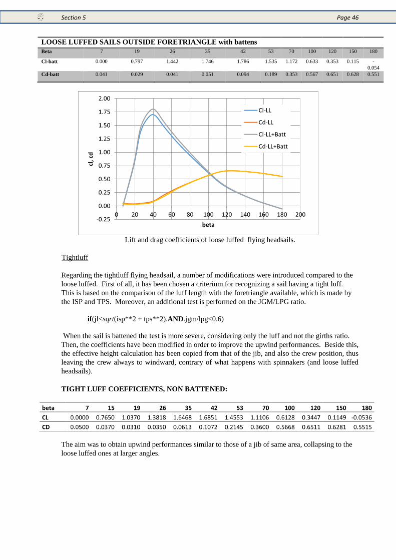
Section 5 Page 46
LOOSE LUFFED SAILS OUTSIDE FORETRIANGLE with battens
Beta 7 19 26 35 42 53 70 100 120 150 180
Cl-batt 0.000 0.797 1.442 1.746 1.786 1.535 1.172 0.633 0.353 0.115 -
0.054
Cd-batt 0.041 0.029 0.041 0.051 0.094 0.189 0.353 0.567 0.651 0.628 0.551
Lift and drag coefficients of loose luffed flying headsails.
Tightluff
Regarding the tightluff flying headsail, a number of modifications were introduced compared to the
loose luffed. First of all, it has been chosen a criterium for recognizing a sail having a tight luff.
This is based on the comparison of the luff length with the foretriangle available, which is made by
the ISP and TPS. Moreover, an additional test is performed on the JGM/LPG ratio.
if(jl<sqrt(isp**2 + tps**2).AND.jgm/lpg<0.6)
When the sail is battened the test is more severe, considering only the luff and not the girths ratio.
Then, the coefficients have been modified in order to improve the upwind performances. Beside this,
the effective height calculation has been copied from that of the jib, and also the crew position, thus
leaving the crew always to windward, contrary of what happens with spinnakers (and loose luffed
headsails).
TIGHT LUFF COEFFICIENTS, NON BATTENED:
beta 7 15 19 26 35 42 53 70 100 120 150 180
CL 0.0000 0.7650 1.0370 1.3818 1.6468 1.6851 1.4553 1.1106 0.6128 0.3447 0.1149 -0.0536
CD 0.0500 0.0370 0.0310 0.0350 0.0613 0.1072 0.2145 0.3600 0.5668 0.6511 0.6281 0.5515
The aim was to obtain upwind performances similar to those of a jib of same area, collapsing to the
loose luffed ones at larger angles.
-0.25
0.00
0.25
0.50
0.75
1.00
1.25
1.50
1.75
2.00
0 20 40 60 80 100 120 140 160 180 200
cl, c
d
beta
Cl-LL
Cd-LL
Cl-LL+Batt
Cd-LL+Batt
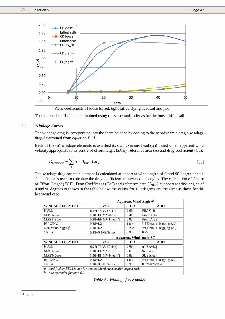
Section 5 Page 47
Aero coefficients of loose luffed, tight luffed flying headsail and jibs.
The battened coefficient are obtained using the same multiplier as for the loose luffed sail.
5.3 Windage Forces
The windage drag is incorporated into the force balance by adding to the aerodynamic drag a windage
drag determined from equation [53].
Each of the (n) windage elements is ascribed its own dynamic head (qn) based on an apparent wind
velocity appropriate to its centre of effort height (ZCE), reference area (A) and drag coefficient (Cd).
n
nREFnWINDAGE CdAqD1
[53]
The windage drag for each element is calculated at apparent wind angles of 0 and 90 degrees and a
shape factor is used to calculate the drag coefficient at intermediate angles. The calculation of Centre
of Effort Height (ZCE), Drag Coefficient (Cd0) and reference area (AREF) at apparent wind angles of
0 and 90 degrees is shown in the table below, the values for 180 degrees are the same as those for the
headwind case.
Apparent. Wind Angle 0
WINDAGE ELEMENT ZCE CD AREF
HULL 0.66(FBAV+Bsin) 0.68 FBAV*B
MAST-Sail HBI+EHM*reef/2 0.4a Front Area
MAST-Bare HBI+EHM*(1-reef)/2 0.8a Front Area
RIGGING HBI+I/2 1.0b I*f(Default. Rigging wt.)
Non round rigging29 HBI+I/2 0.25b I*f(Default. Rigging wt.)
CREW HBI+0.5+B/2sin 0.9 0.25
Apparent. Wind Angle 90
WINDAGE ELEMENT ZCE CD AREF
HULL 0.66(FBAV+Bsin) 0.68 f(HSA*L,)
MAST-Sail HBI+EHM*reef/2 0.6a Side Area
MAST-Bare HBI+EHM*(1-reef)/2 0.8a Side Area
RIGGING HBI+I/2 1.0b I*f(Default. Rigging wt.)
CREW HBI+0.5+B/2sin 0.9 0.5*Mvblcrew
a modified by EDM factor for non standard mast section aspect ratio. b plus spreader factor = 0.2
Table 8 - Windage force model
29 2011
-0.25
0.00
0.25
0.50
0.75
1.00
1.25
1.50
1.75
2.00
0 10 20 30 40 50
cd, c
l
beta
CL looseluffed sailsCD looseluffed sailsCL JIB_Hi
CD JIB_Hi
CL_tight
Section 5 Page 48
Hull side area (HSA)
n
FreeboardHSA0
dl [54]
where n = number of measurement stations.
5.3.1 Rigging
The drag of the rigging wire is calculated based on the default rigging weight. The square root converts
wire cross-sectional area to wire diameter, and the factor of 2 means four stays.
/_//__0.42___ densitySteelMIRigngDefltWTdwireRiggingofDiameter [55]
WireRiggingofDiameterIwindageWireRiggingArea ______ [56]
windageFactorspreaderWireRiggingCDWireRiggingCd __1____0 [57]
5.3.1.1 Spreaders
If the rig has bona-fide spreaders their drag is added in as a multiplier as shown in equation
[57]Error! Reference source not found., where spreader_Factor_windage is set to 0.2.
5.4 Total Aerodynamic Lift and Drag
The next phase is to combine the individual sail’s characteristics to produce a set of lift and drag
coefficients that describe the aerodynamic behavior of the entire rig.
This is accomplished by a weighted superposition of the individual sail force coefficients at each
apparent wind angle. This process is described in more detail in section 7.4.1.
The weight given to each sail’s coefficients during this process is proportional to the product of its
area and the “blanketing” factor, which modifies the individual sails coefficients depending on the
apparent wind angle. After summing the weighted coefficients the total is normalized with respect to
the reference sail area (AREF).
When calculating the collective vertical centre of force the weight given to each sail’s contribution is
proportional to the product of the area, the blanketing factor, and the total force coefficient.
The induced drag coefficient is calculated from knowledge of the effective rig height. (HE)
2
2
1
E
REF
H
AClCd
[58]
The effective rig height is calculated from the sail plan geometry at each iteration of the VPP through
the aerodynamic force calculation loop.
The effective rig height is a function of:
- the mainsail roach
- the relative positions of the mainsail head and the jib head expressed as “fractionality” and
- the overlap of the headsail
5.4.1 Lift and Drag of complete sail set
The aggregate maximum lift and linear parasite drag coefficients are the sum of each sail component’s
contribution normalized by reference area, and modified by a blanketing function Bi:
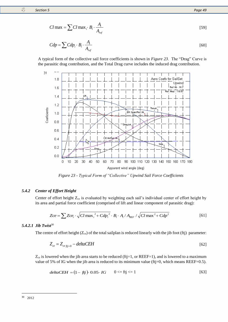
Section 5 Page 49
ref
iii
A
ABClCl maxmax [59]
ref
iii
A
ABCdpCdp [60]
A typical form of the collective sail force coefficients is shown in Figure 23. The “Drag” Curve is
the parasitic drag contribution, and the Total Drag curve includes the induced drag contribution.
Figure 23 - Typical Form of “Collective” Upwind Sail Force Coefficients
5.4.2 Center of Effort Height
Center of effort height Zce is evaluated by weighting each sail’s individual center of effort height by
its area and partial force coefficient (comprised of lift and linear component of parasitic drag):
2222max//max CdpClAABCdpClZceZce REFiiiii [61]
5.4.2.1 Jib Twist30
The centre of effort height (Zce) of the total sailplan is reduced linearly with the jib foot (ftj) parameter:
deltaCEHZZftjcece 0 [62]
Zce is lowered when the jib area starts to be reduced (ftj=1, or REEF=1), and is lowered to a maximum
value of 5% of IG when the jib area is reduced to its minimum value (ftj=0, which means REEF=0.5).
IGftjdeltaCEH 05.01 0 <= ftj <= 1 [63]
30 2012
Section 5 Page 50
5.4.3 Induced Drag
In order to calculate the induced drag component an efficiency coefficient is derived. The efficiency
coefficient is such that when multiplied by the collective lift coefficient squared it yields the collective
induced drag of the sails. The efficiency coefficient is comprised of 2 parts;
The 2 dimensional part describing the increase of viscous drag that occurs as the sail produces more
lift,
and the “induced drag” which depends on the effective rig height.
5.4.3.1 Quadratic Parasite Drag
The viscous drag of the sails varies according to the square of the lift coefficient. This quadratic
parasite drag coefficient KPP is the sums of the individual sails contributions:
22
max//max ClAABClKPPKPP refiiii [64]
5.4.3.2 Effective rig height
Three parameters - “fractionality”, “overlap” and “roach”- are determined in order to calculate the
Effective rig height which determines the induced drag of the sails.
Fractionality = Icurrent/(Pcurrent + BAS)
Overlap = LPGcurrent/J
Roach = Mainsail Area /(P x E / 2) -1
The influence of sail plan geometry is first calculated to derive a corrected effective span coefficient
as follows:
1.1075.031.068.05.02.008.01.1__ overlapityfractionalRoachcorrspaneff [65]
The effective span coefficient is approximately 1.10 with a masthead rig (fractionality = 1.0) and 150%
overlap genoa.
The effective span coefficient is then further modified to reflect the fact that as the sails are eased at
wider apparent wind angles the effective span is reduced as the sealing of the jib and the hull is lost
and the sail interactions become less favourable.
becorrspaneffcheffUpwind 2.08.0__ [66]
bespicheffcheff Downwind 1.00.1max__ [67]
The term be varies from 1 to zero as apparent wind angle widens from 30 to 90 degrees (Figure 24).
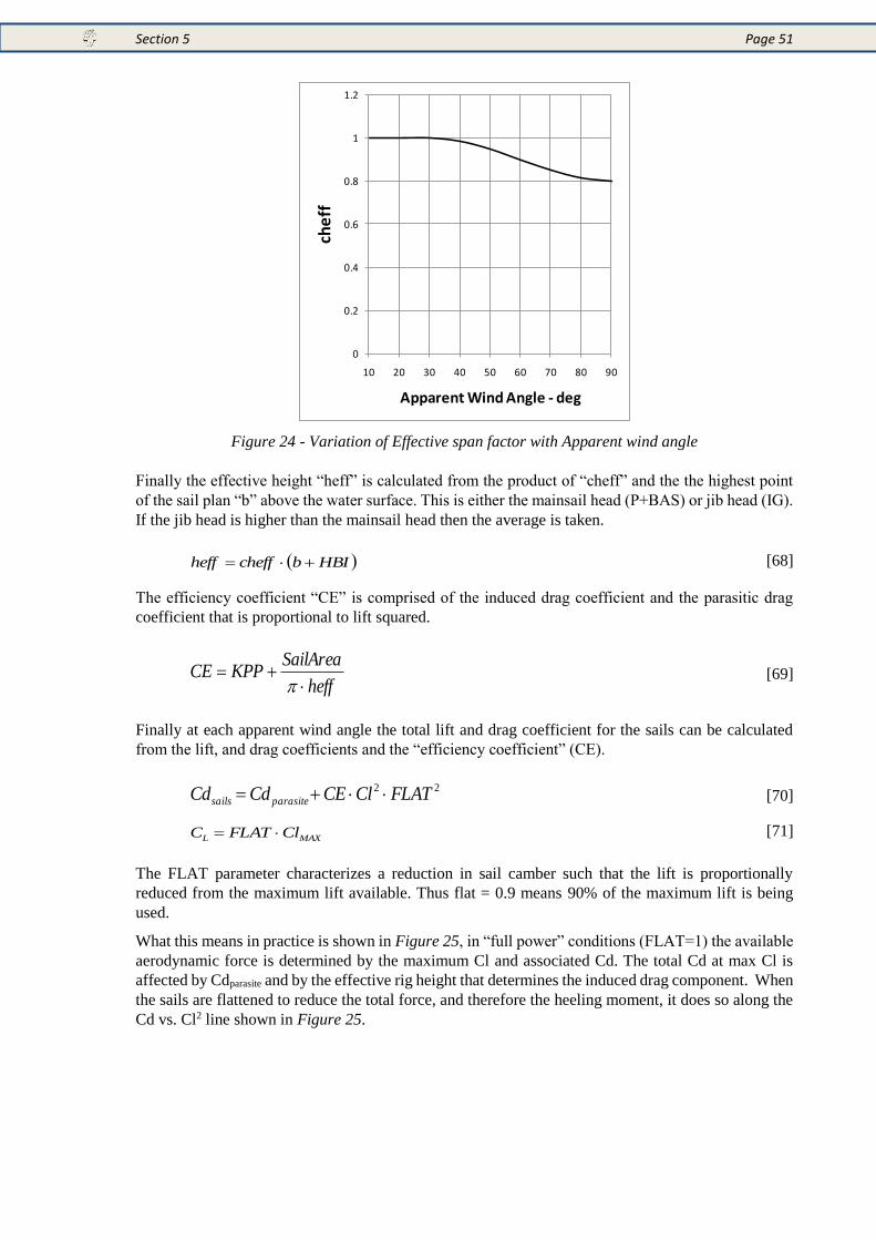
Section 5 Page 51
Figure 24 - Variation of Effective span factor with Apparent wind angle
Finally the effective height “heff” is calculated from the product of “cheff” and the the highest point
of the sail plan “b” above the water surface. This is either the mainsail head (P+BAS) or jib head (IG).
If the jib head is higher than the mainsail head then the average is taken.
HBIbcheffheff [68]
The efficiency coefficient “CE” is comprised of the induced drag coefficient and the parasitic drag
coefficient that is proportional to lift squared.
heff
SailAreaKPPCE
[69]
Finally at each apparent wind angle the total lift and drag coefficient for the sails can be calculated
from the lift, and drag coefficients and the “efficiency coefficient” (CE).
22 FLATClCECdCd parasitesails [70]
MAXL ClFLATC [71]
The FLAT parameter characterizes a reduction in sail camber such that the lift is proportionally
reduced from the maximum lift available. Thus flat = 0.9 means 90% of the maximum lift is being
used.
What this means in practice is shown in Figure 25, in “full power” conditions (FLAT=1) the available
aerodynamic force is determined by the maximum Cl and associated Cd. The total Cd at max Cl is
affected by Cdparasite and by the effective rig height that determines the induced drag component. When
the sails are flattened to reduce the total force, and therefore the heeling moment, it does so along the
Cd vs. Cl2 line shown in Figure 25.
0
0.2
0.4
0.6
0.8
1
1.2
10 20 30 40 50 60 70 80 90
che
ff
Apparent Wind Angle - deg
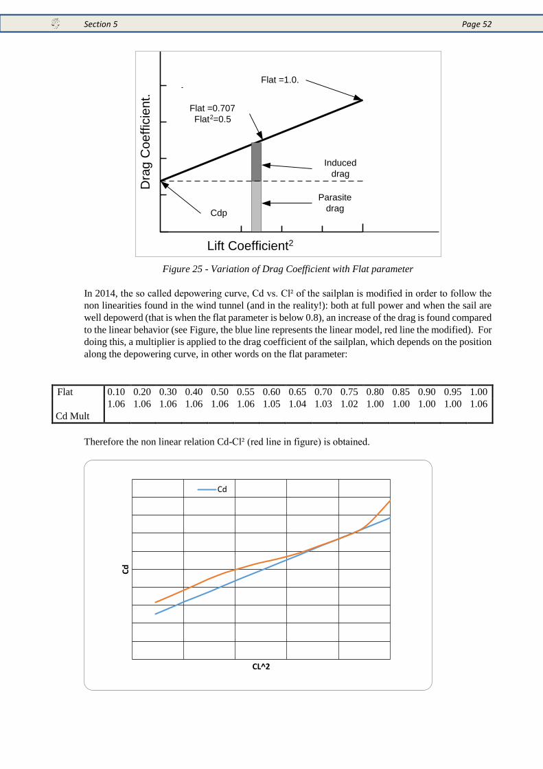
Section 5 Page 52
Figure 25 - Variation of Drag Coefficient with Flat parameter
In 2014, the so called depowering curve, Cd vs. Cl² of the sailplan is modified in order to follow the
non linearities found in the wind tunnel (and in the reality!): both at full power and when the sail are
well depowerd (that is when the flat parameter is below 0.8), an increase of the drag is found compared
to the linear behavior (see Figure, the blue line represents the linear model, red line the modified). For
doing this, a multiplier is applied to the drag coefficient of the sailplan, which depends on the position
along the depowering curve, in other words on the flat parameter:
Flat 0.10 0.20 0.30 0.40 0.50 0.55 0.60 0.65 0.70 0.75 0.80 0.85 0.90 0.95 1.00
Cd Mult
1.06
0
1.06
0
1.06
0
1.06
0
1.06
0
1.06
0
1.05
5
1.04
8
1.03
5
1.02
0
1.00
8
1.00
2
1.00
0
1.00
4
1.06
0
Therefore the non linear relation Cd-Cl² (red line in figure) is obtained.
Dra
g C
oe
ffic
ien
t.
Lift Coefficient2
Flat =1.0.
Flat =0.707
Flat2=0.5
Cdp
Induced
drag
Parasite
drag
Cd
CL^2
Cd
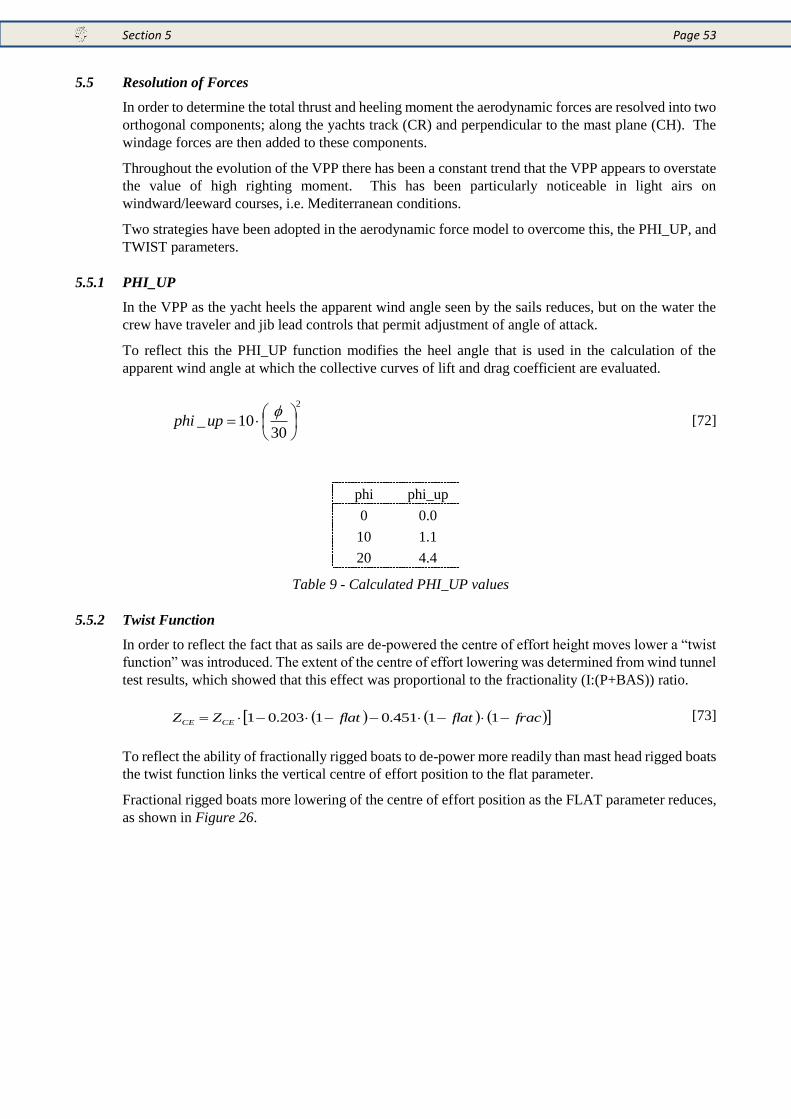
Section 5 Page 53
5.5 Resolution of Forces
In order to determine the total thrust and heeling moment the aerodynamic forces are resolved into two
orthogonal components; along the yachts track (CR) and perpendicular to the mast plane (CH). The
windage forces are then added to these components.
Throughout the evolution of the VPP there has been a constant trend that the VPP appears to overstate
the value of high righting moment. This has been particularly noticeable in light airs on
windward/leeward courses, i.e. Mediterranean conditions.
Two strategies have been adopted in the aerodynamic force model to overcome this, the PHI_UP, and
TWIST parameters.
5.5.1 PHI_UP
In the VPP as the yacht heels the apparent wind angle seen by the sails reduces, but on the water the
crew have traveler and jib lead controls that permit adjustment of angle of attack.
To reflect this the PHI_UP function modifies the heel angle that is used in the calculation of the
apparent wind angle at which the collective curves of lift and drag coefficient are evaluated.
2
3010_
upphi [72]
phi phi_up
0 0.0
10 1.1
20 4.4
Table 9 - Calculated PHI_UP values
5.5.2 Twist Function
In order to reflect the fact that as sails are de-powered the centre of effort height moves lower a “twist
function” was introduced. The extent of the centre of effort lowering was determined from wind tunnel
test results, which showed that this effect was proportional to the fractionality (I:(P+BAS)) ratio.
fracflatflatZZ CECE 11451.01203.01 [73]
To reflect the ability of fractionally rigged boats to de-power more readily than mast head rigged boats
the twist function links the vertical centre of effort position to the flat parameter.
Fractional rigged boats more lowering of the centre of effort position as the FLAT parameter reduces,
as shown in Figure 26.
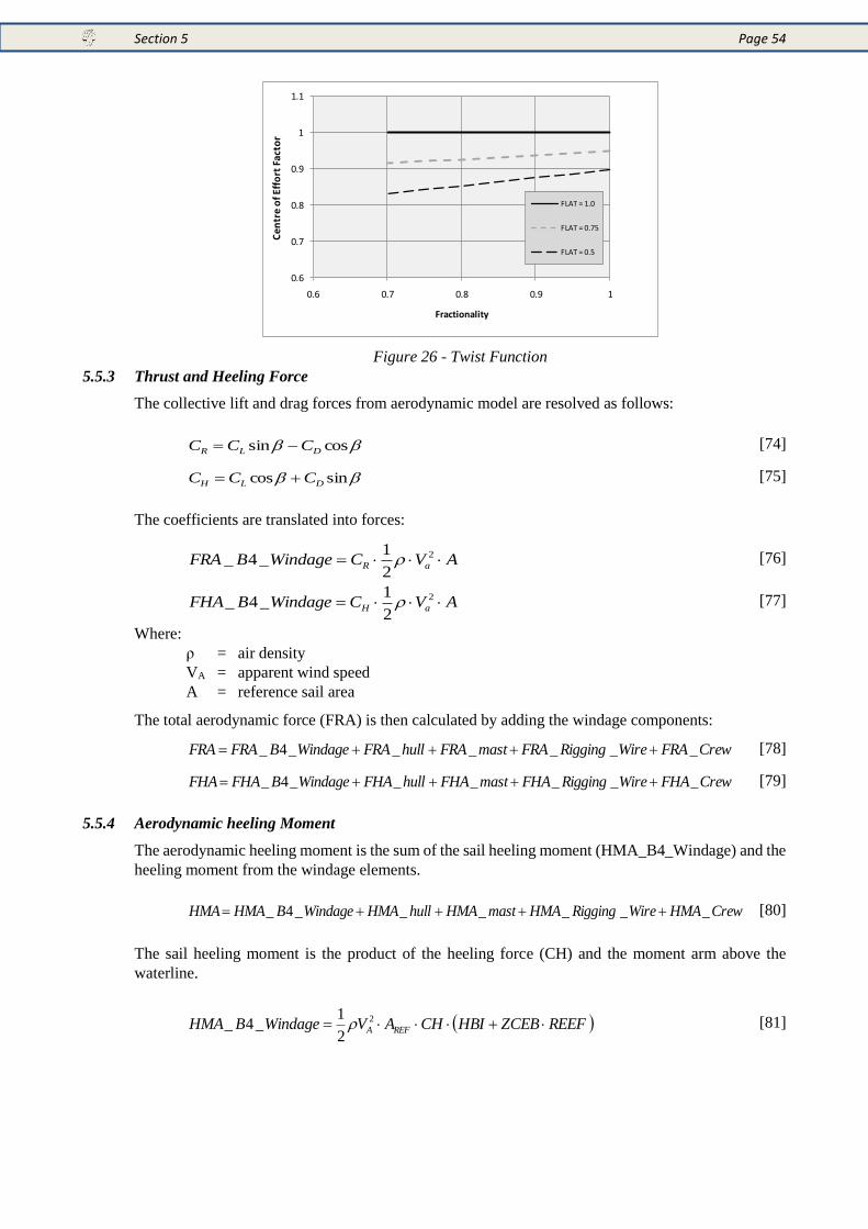
Section 5 Page 54
Figure 26 - Twist Function
5.5.3 Thrust and Heeling Force
The collective lift and drag forces from aerodynamic model are resolved as follows:
cossin DLR CCC [74]
sincos DLH CCC [75]
The coefficients are translated into forces:
AVCWindageBFRA aR 2
2
1_4_ [76]
AVCWindageBFHA aH 2
2
1_4_ [77]
Where:
ρ = air density
VA = apparent wind speed
A = reference sail area
The total aerodynamic force (FRA) is then calculated by adding the windage components:
CrewFRAWireRiggingFRAmastFRAhullFRAWindageBFRAFRA ______4_ [78]
CrewFHAWireRiggingFHAmastFHAhullFHAWindageBFHAFHA ______4_ [79]
5.5.4 Aerodynamic heeling Moment
The aerodynamic heeling moment is the sum of the sail heeling moment (HMA_B4_Windage) and the
heeling moment from the windage elements.
CrewHMAWireRiggingHMAmastHMAhullHMAWindageBHMAHMA ______4_ [80]
The sail heeling moment is the product of the heeling force (CH) and the moment arm above the
waterline.
REEFZCEBHBICHAVWindageBHMA REFA 2
2
1_4_ [81]
0.6
0.7
0.8
0.9
1
1.1
0.6 0.7 0.8 0.9 1
Cen
tre
of E
ffo
rt F
acto
r
Fractionality
FLAT = 1.0
FLAT = 0.75
FLAT = 0.5
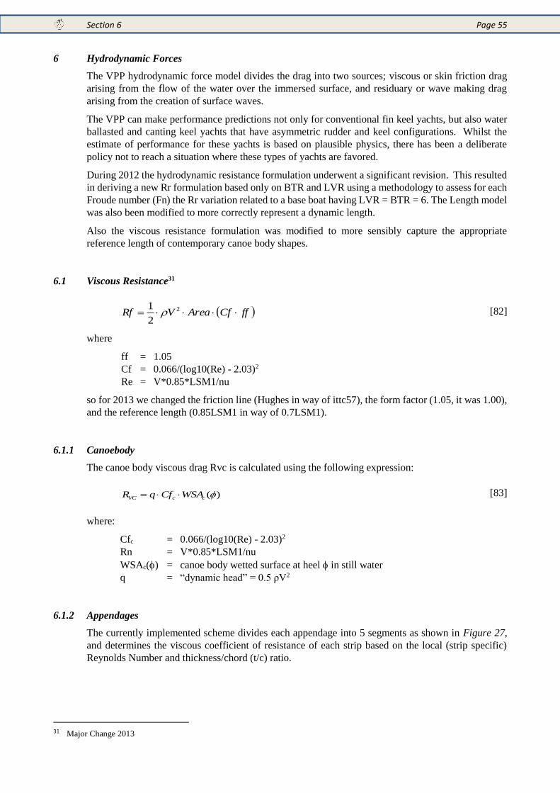
Section 6 Page 55
6 Hydrodynamic Forces
The VPP hydrodynamic force model divides the drag into two sources; viscous or skin friction drag
arising from the flow of the water over the immersed surface, and residuary or wave making drag
arising from the creation of surface waves.
The VPP can make performance predictions not only for conventional fin keel yachts, but also water
ballasted and canting keel yachts that have asymmetric rudder and keel configurations. Whilst the
estimate of performance for these yachts is based on plausible physics, there has been a deliberate
policy not to reach a situation where these types of yachts are favored.
During 2012 the hydrodynamic resistance formulation underwent a significant revision. This resulted
in deriving a new Rr formulation based only on BTR and LVR using a methodology to assess for each
Froude number (Fn) the Rr variation related to a base boat having LVR = BTR = 6. The Length model
was also been modified to more correctly represent a dynamic length.
Also the viscous resistance formulation was modified to more sensibly capture the appropriate
reference length of contemporary canoe body shapes.
6.1 Viscous Resistance31
ffCfAreaVRf 2
2
1 [82]
where
ff = 1.05
Cf = 0.066/(log10(Re) - 2.03)2
Re = V*0.85*LSM1/nu
so for 2013 we changed the friction line (Hughes in way of ittc57), the form factor (1.05, it was 1.00),
and the reference length (0.85LSM1 in way of 0.7LSM1).
6.1.1 Canoebody
The canoe body viscous drag Rvc is calculated using the following expression:
)(ccVC WSACfqR [83]
where:
Cfc = 0.066/(log10(Re) - 2.03)2
Rn = V*0.85*LSM1/nu
WSAc() = canoe body wetted surface at heel in still water
q = “dynamic head” = 0.5 ρV2
6.1.2 Appendages
The currently implemented scheme divides each appendage into 5 segments as shown in Figure 27,
and determines the viscous coefficient of resistance of each strip based on the local (strip specific)
Reynolds Number and thickness/chord (t/c) ratio.
31 Major Change 2013
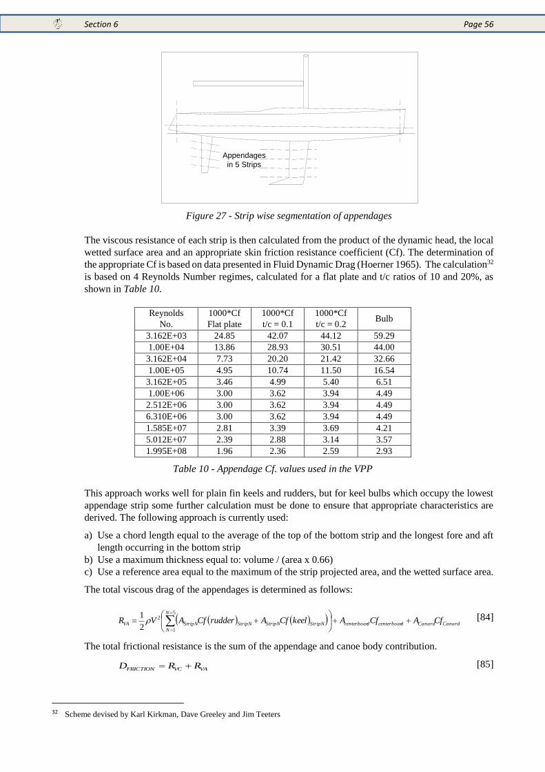
Section 6 Page 56
Figure 27 - Strip wise segmentation of appendages
The viscous resistance of each strip is then calculated from the product of the dynamic head, the local
wetted surface area and an appropriate skin friction resistance coefficient (Cf). The determination of
the appropriate Cf is based on data presented in Fluid Dynamic Drag (Hoerner 1965). The calculation32
is based on 4 Reynolds Number regimes, calculated for a flat plate and t/c ratios of 10 and 20%, as
shown in Table 10.
Reynolds
No.
1000*Cf
Flat plate
1000*Cf
t/c = 0.1
1000*Cf
t/c = 0.2
Bulb
3.162E+03 24.85 42.07 44.12 59.29
1.00E+04 13.86 28.93 30.51 44.00
3.162E+04 7.73 20.20 21.42 32.66
1.00E+05 4.95 10.74 11.50 16.54
3.162E+05 3.46 4.99 5.40 6.51
1.00E+06 3.00 3.62 3.94 4.49
2.512E+06 3.00 3.62 3.94 4.49
6.310E+06 3.00 3.62 3.94 4.49
1.585E+07 2.81 3.39 3.69 4.21
5.012E+07 2.39 2.88 3.14 3.57
1.995E+08 1.96 2.36 2.59 2.93
Table 10 - Appendage Cf. values used in the VPP
This approach works well for plain fin keels and rudders, but for keel bulbs which occupy the lowest
appendage strip some further calculation must be done to ensure that appropriate characteristics are
derived. The following approach is currently used:
a) Use a chord length equal to the average of the top of the bottom strip and the longest fore and aft
length occurring in the bottom strip
b) Use a maximum thickness equal to: volume / (area x 0.66)
c) Use a reference area equal to the maximum of the strip projected area, and the wetted surface area.
The total viscous drag of the appendages is determined as follows:
CanardCanarddcenterboardcenterboar
N
N
StripNStripNStripNStripNVA CfACfAkeelCfArudderCfAVR
5
1
2
2
1 [84]
The total frictional resistance is the sum of the appendage and canoe body contribution.
VAVCFRICTION RRD [85]
32 Scheme devised by Karl Kirkman, Dave Greeley and Jim Teeters
Appendages
in 5 Strips
Section 6 Page 57
6.1.2.1 Double rudders (2010)
The Offset file has now been configured to accept double rudder configurations as detailed in
Appendix A. The viscous drag is calculated according to Table 10, with no velocity deficit for the keel
wake. The immersed wetted area is calculated at each heel angle assuming an undisturbed static
waterplane.
6.1.2.2 Centreboards
Because centerboards are often not as well refined as keel fins a different drag formulation33 is adopted:
cbAVdragdCenterboar 2
2
1006.0_ [86]
44
22)_(__
CBRCCBMCCBTCECMAdCenterboarAreaWetted cb
[87]
where:
ρ = Water density
ECM = Centre board extension
CBTC = Centerboard tip chord
CBMC = Centerboard mid chord
CBRC = Centerboard root chord
If there is no data for centerboard chord then the following formula is applied.
26.02___ ECMAdCenterboarAreaWetted cb [88]
6.1.2.3 Dagger Boards, Bilge Boards
Bilge boards and dagger boards are treated as per Table 10 based on their area and mean chord length.
6.1.2.4 Trim Tabs
The use of a trim tab to reduce the viscous drag of the keel fin by shifting the viscous “drag bucket”
to higher lift coefficient is reflected in a formula that reduces the viscous drag coefficient for a keel
with a trim tab34.
Aq
SideforceCltCoefficienLift
75.0__ [89]
0034.000029.00097.0__ 2 ClClCdtCoefficienDrag [90]
0034.033.0_ CddiffCd [91]
Where A is the keel area and q is the dynamic head 0.5 ρV2.
Cd_diff is subtracted from the keel strip friction drag coefficient.
33 1987 ERFXNEW.FOR, MODLDIM2.FOR 34 The form of the code reflects that the drag reduction has been reduced over time because the original formulation was regarded as
too punitive in terms of handicap.
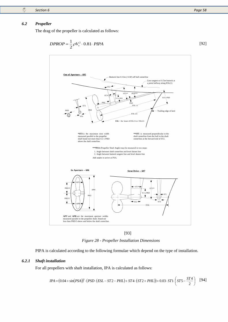
Section 6 Page 58
6.2 Propeller
The drag of the propeller is calculated as follows:
PIPAVDPROP s 81.02
1 2 [92]
[93]
Figure 28 - Propeller Installation Dimensions
PIPA is calculated according to the following formulae which depend on the type of installation.
6.2.1 Shaft installation
For all propellers with shaft installation, IPA is calculated as follows:
2
45103.0242sin04.0
3 STSTSTPHLSTSTPHLSTESLPSDPSAIPA [94]
Out of Aperture -- 605
Strut Drive -- 607
0.3 x PRD
ST3*
ST2
ST1
ST4
EDL
ST5**
PRD
PRD/3
PRD/3
APT
APB
APT and APB are the maximum aperture widths
measured parallel to the propeller shaft, found not
less than PRD/3 above and below the shaft centerline.
In Aperture -- 606
APH
Buttock line 0.15m ( 0.50') off hull centerline
*ST3 is the maximum strut width
measured parallel to the propeller
shaft found not more than 0.3 x PRD
above the shaft centerline.
**ST5 is measured perpendicular to the
shaft centerline from the hull to the shaft
centerline at the forward end of ST2.
***PSA (Propeller Shaft Angle) may be measured in two steps:
1. Angle between shaft centerline and level datum line
2. Angle between buttock tangent line and level datum line
Add angles to arrive at PSA.
Line tangent to 0.15m buttock at
a point halfway along ESL(1)
Trailing edge of keel
ST1
ST4
PHD PRD
PHL
ST3*
ST2
ESL = the lesser of ESL(1) or ESL(2)
ST5**
PSD
PSA***
ESL (1)
ESL (2)
8.0 x PSD0.3 x PRD
Section 6 Page 59
6.2.1.1 Folding and feathering 2 blade
29.065.0 PHDIPAPIPA [95]
For a folding propeller PHD shall not be taken greater than 3.5xPSD in the above formula.
6.2.1.2 Folding and feathering 3 blade
29.070.0 PHDIPAPIPA [96]
For a feathering propeller PHD shall not be taken greater than 4.0*PSD in the above formula.
6.2.1.3 Solid 2 blade
210.0 PRDIPAPIPA [97]
6.2.1.4 Solid 3 and more blades
212.0 PRDIPAPIPA [98]
If ESL is less than PRD, PIPA shall be multiplied by 0.5.
6.2.2 Strut drive
PIPA shall be determined as follows:
6.2.2.1 Folding and feathering 2 blade
2)48.0(4.045.05106.0 STSTSTSTPIPA [99]
6.2.2.2 Folding and Feathering 3 Blade
2)48.0(42.045.05106.0 STSTSTSTPIPA [100]
6.2.2.3 Solid 2 Blade
210.045.05106.0 PRDSTSTSTPIPA [101]
6.2.2.4 Solid 3+ Blades
212.045.05106.0 PRDSTSTSTPIPA [102]
Notes:
1. For any strut drive, if EDL is less than 1.5 * PRD, PIPA shall be multiplied by 0.5.
2. The shape of the strut may be modified, but the full functionality of the standard model must be
retained and ST1-ST4 values may not be reduced below the unmodified standard dimensions. For
handicapping purposes ST1-ST4 shall not be taken bigger than the unmodified standard
dimensions.
3. ST4 shall be measured at the aft end of the hub instead of at the point of maximum projected area,
better representing the flow separation drag.
4. An upper ST4 limit will be used for the PIPA. This limit depends on the L of the yacht. The
maximum is defined by a curve of values just above those typical of most common production
units, faired over an ample length range. The upper limit for ST4 is thus defined as the lesser of:
05.0015.00011.0104 235 LLL or 0.2 (but never less than 0.1) [103]
6.2.3 In an aperture
Section 6 Page 60
For propellers of any type installed in an aperture PIPA shall be taken as the least of the values
determined by the formulae:
207.0 PRDPIPA [104]
2
407.0
APTPIPA [105]
2
125.107.0
APHPIPA [106]
2
407.0
APBPIPA [107]
6.2.4 Tractor propellers
For tractor propellers of any type installed out of aperture PIPA shall be zero.
6.2.5 Twin screws
IMS has an input to signify twin propeller installations. If this is indicated, PIPA is doubled for any
type of installation or propeller.
6.3 Residuary Resistance35
The calculation of the wave-making or residuary resistance is based on the calculation of a residuary
resistance coefficient at preset values of Froude Number (Fn). The Fn is a non-dimensional speed
based on the yachts Dynamic Length LDyn
Dyn
nLg
VF
[108]
The hull is the main element of the residuary resistance, with a small contribution from the appendages.
Recognizing that previous attempts to accurately calculate the effect of several hull parameters such
as Prismatic Coefficient, Longitudinal Center of Buoyancy (LCB) and water plane area coefficient
have led to undesirable type-formed hull shapes and that this trend could not be addressed within the
existing model, it was decided to simplify the input parameters accounting for 2 main parameters only:
dynamic Length-Volume ratio (LVR), and Beam to Canoe-body-draft ratio (BTR) to avoid as much
as possible any type-forming. The effects of hull volume distribution are still captured by the use of
the traditional integrated lengths.
6.3.1 Resistance Surfaces
The Rr drag curve for the canoe body is formed by the extraction of drag values at 24 Froude numbers
(Fn) from surfaces of BTR and dynamic LVR and ranging from Fn 0.125 up to Fn 0.7.
The Froude number used also incorporates dynamic length. For speeds outside this range the resistance
is extrapolated. The BTR and LVR ranges of the surface are 2.5 to 9 and 3 to 9 respectively and outside
this range the value defaults to that of the closest point of the surface.
The LVR-BTR surfaces are very similar to the example plots below and the points from which they
are derived can be downloaded in .CSV file format from www.orc.org/rules.
35 Major Revision 2013
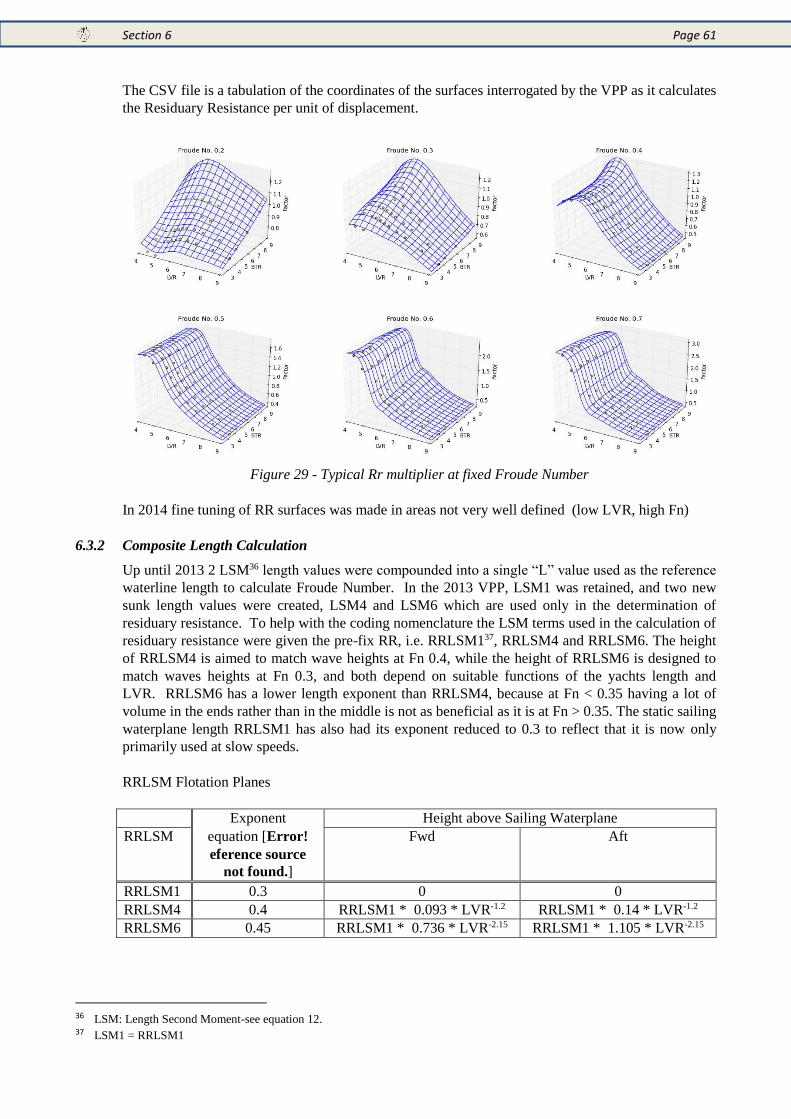
Section 6 Page 61
The CSV file is a tabulation of the coordinates of the surfaces interrogated by the VPP as it calculates
the Residuary Resistance per unit of displacement.
Figure 29 - Typical Rr multiplier at fixed Froude Number
In 2014 fine tuning of RR surfaces was made in areas not very well defined (low LVR, high Fn)
6.3.2 Composite Length Calculation
Up until 2013 2 LSM36 length values were compounded into a single “L” value used as the reference
waterline length to calculate Froude Number. In the 2013 VPP, LSM1 was retained, and two new
sunk length values were created, LSM4 and LSM6 which are used only in the determination of
residuary resistance. To help with the coding nomenclature the LSM terms used in the calculation of
residuary resistance were given the pre-fix RR, i.e. RRLSM137, RRLSM4 and RRLSM6. The height
of RRLSM4 is aimed to match wave heights at Fn 0.4, while the height of RRLSM6 is designed to
match waves heights at Fn 0.3, and both depend on suitable functions of the yachts length and
LVR. RRLSM6 has a lower length exponent than RRLSM4, because at Fn < 0.35 having a lot of
volume in the ends rather than in the middle is not as beneficial as it is at Fn > 0.35. The static sailing
waterplane length RRLSM1 has also had its exponent reduced to 0.3 to reflect that it is now only
primarily used at slow speeds.
RRLSM Flotation Planes
Exponent Height above Sailing Waterplane
RRLSM equation [Error!
eference source
not found.]
Fwd Aft
RRLSM1 0.3 0 0
RRLSM4 0.4 RRLSM1 * 0.093 * LVR-1.2 RRLSM1 * 0.14 * LVR-1.2
RRLSM6 0.45 RRLSM1 * 0.736 * LVR-2.15 RRLSM1 * 1.105 * LVR-2.15
36 LSM: Length Second Moment-see equation 12. 37 LSM1 = RRLSM1
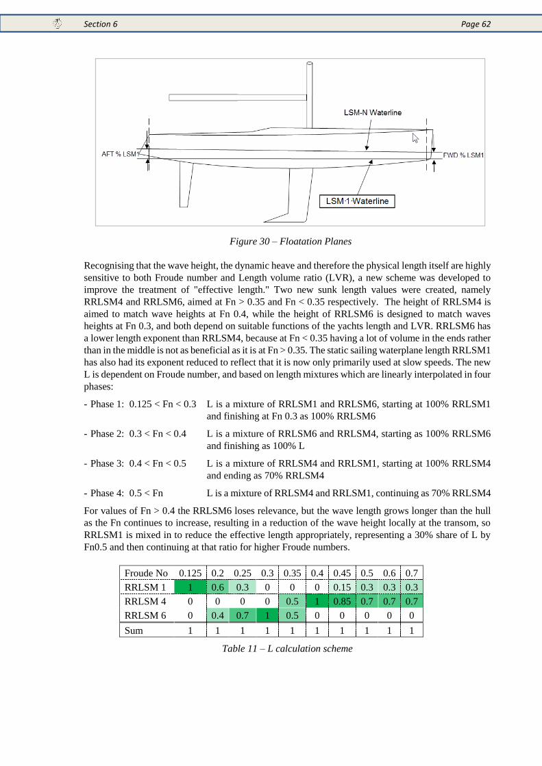
Section 6 Page 62
Figure 30 – Floatation Planes
Recognising that the wave height, the dynamic heave and therefore the physical length itself are highly
sensitive to both Froude number and Length volume ratio (LVR), a new scheme was developed to
improve the treatment of "effective length." Two new sunk length values were created, namely
RRLSM4 and RRLSM6, aimed at Fn > 0.35 and Fn < 0.35 respectively. The height of RRLSM4 is
aimed to match wave heights at Fn 0.4, while the height of RRLSM6 is designed to match waves
heights at Fn 0.3, and both depend on suitable functions of the yachts length and LVR. RRLSM6 has
a lower length exponent than RRLSM4, because at Fn < 0.35 having a lot of volume in the ends rather
than in the middle is not as beneficial as it is at Fn > 0.35. The static sailing waterplane length RRLSM1
has also had its exponent reduced to reflect that it is now only primarily used at slow speeds. The new
L is dependent on Froude number, and based on length mixtures which are linearly interpolated in four
phases:
- Phase 1: 0.125 < Fn < 0.3 L is a mixture of RRLSM1 and RRLSM6, starting at 100% RRLSM1
and finishing at Fn 0.3 as 100% RRLSM6
- Phase 2: 0.3 < Fn < 0.4 L is a mixture of RRLSM6 and RRLSM4, starting as 100% RRLSM6
and finishing as 100% L
- Phase 3: 0.4 < Fn < 0.5 L is a mixture of RRLSM4 and RRLSM1, starting at 100% RRLSM4
and ending as 70% RRLSM4
- Phase 4: 0.5 < Fn L is a mixture of RRLSM4 and RRLSM1, continuing as 70% RRLSM4
For values of Fn > 0.4 the RRLSM6 loses relevance, but the wave length grows longer than the hull
as the Fn continues to increase, resulting in a reduction of the wave height locally at the transom, so
RRLSM1 is mixed in to reduce the effective length appropriately, representing a 30% share of L by
Fn0.5 and then continuing at that ratio for higher Froude numbers.
Froude No 0.125 0.2 0.25 0.3 0.35 0.4 0.45 0.5 0.6 0.7
RRLSM 1 1 0.6 0.3 0 0 0 0.15 0.3 0.3 0.3
RRLSM 4 0 0 0 0 0.5 1 0.85 0.7 0.7 0.7
RRLSM 6 0 0.4 0.7 1 0.5 0 0 0 0 0
Sum 1 1 1 1 1 1 1 1 1 1
Table 11 – L calculation scheme
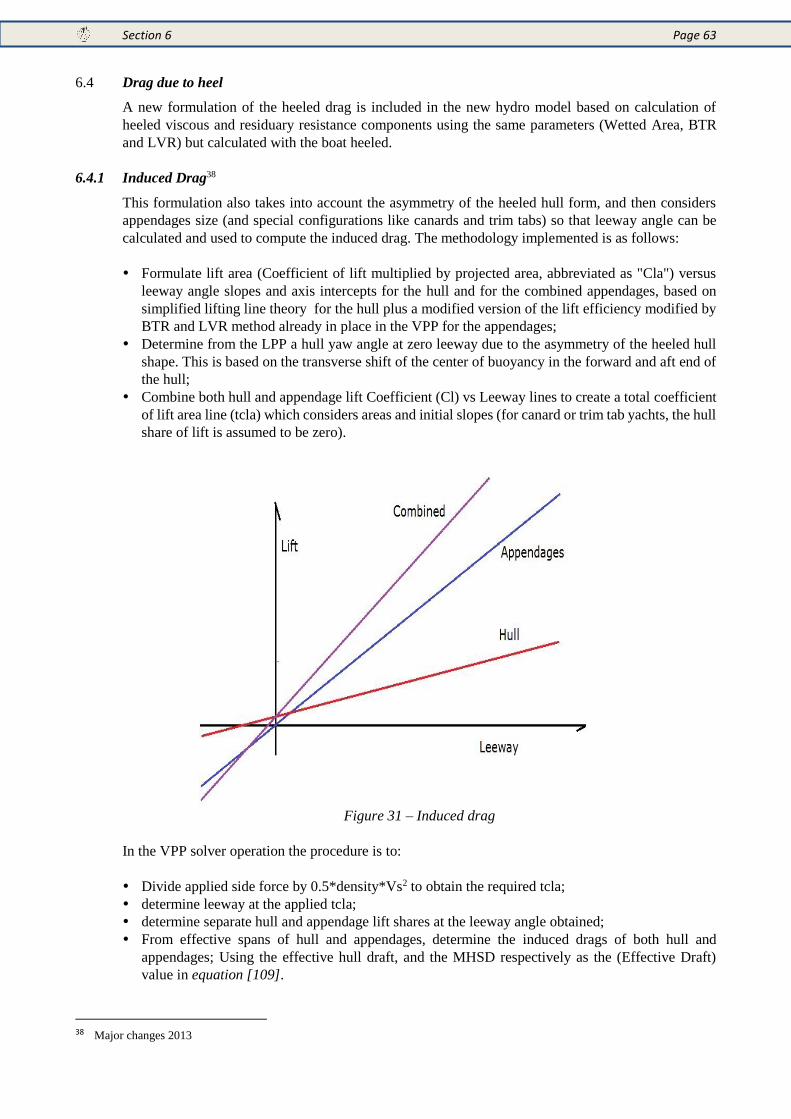
Section 6 Page 63
6.4 Drag due to heel
A new formulation of the heeled drag is included in the new hydro model based on calculation of
heeled viscous and residuary resistance components using the same parameters (Wetted Area, BTR
and LVR) but calculated with the boat heeled.
6.4.1 Induced Drag38
This formulation also takes into account the asymmetry of the heeled hull form, and then considers
appendages size (and special configurations like canards and trim tabs) so that leeway angle can be
calculated and used to compute the induced drag. The methodology implemented is as follows:
Formulate lift area (Coefficient of lift multiplied by projected area, abbreviated as "Cla") versus
leeway angle slopes and axis intercepts for the hull and for the combined appendages, based on
simplified lifting line theory for the hull plus a modified version of the lift efficiency modified by
BTR and LVR method already in place in the VPP for the appendages;
Determine from the LPP a hull yaw angle at zero leeway due to the asymmetry of the heeled hull
shape. This is based on the transverse shift of the center of buoyancy in the forward and aft end of
the hull;
Combine both hull and appendage lift Coefficient (Cl) vs Leeway lines to create a total coefficient
of lift area line (tcla) which considers areas and initial slopes (for canard or trim tab yachts, the hull
share of lift is assumed to be zero).
Figure 31 – Induced drag
In the VPP solver operation the procedure is to:
Divide applied side force by 0.5*density*Vs2 to obtain the required tcla;
determine leeway at the applied tcla;
determine separate hull and appendage lift shares at the leeway angle obtained;
From effective spans of hull and appendages, determine the induced drags of both hull and
appendages; Using the effective hull draft, and the MHSD respectively as the (Effective Draft)
value in equation [109].
38 Major changes 2013
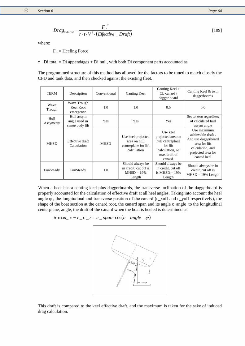
Section 6 Page 64
DraftEffectiveVtr
FDrag H
induced_2
2
[109]
where:
FH = Heeling Force
Di total = Di appendages + Di hull, with both Di component parts accounted as
The programmed structure of this method has allowed for the factors to be tuned to match closely the
CFD and tank data, and then checked against the existing fleet.
TERM
Description
Conventional
Canting Keel
Canting Keel +
CL canard /
dagger board
Canting Keel & twin
daggerboards
Wave
Trough
Wave Trough
Keel Root
emergence
1.0
1.0
0.5
0.0
Hull
Assymetry
Hull assym
angle used in
canoe body lift
Yes
Yes
Yes
Set to zero regardless
of calculated hull
assym angle
MHSD
Effective draft
Calculation
MHSD
Use keel projected
area on hull
centreplane for lift
calculation
Use keel
projected area on
hull centreplane
for lift
calculation, or
max draft of
canard.
Use maximum
achievable draft ,
And use daggerboard
area for lift
calculation, and
projected area for
canted keel
FunSteady
FunSteady
1.0
Should always be
in credit, cut off is
MHSD = 19%
Length
Should always be
in credit, cut off
is MHSD = 19%
Length
Should always be in
credit, cut off is
MHSD = 19% Length
When a boat has a canting keel plus daggerboards, the transverse inclination of the daggerboard is
properly accounted for the calculation of effective draft at all heel angles. Taking into account the heel
angle φ , the longitudinal and transverse position of the canard (c_xoff and c_yoff respectively), the
shape of the boat section at the canard root, the canard span and its angle c_angle to the longitudinal
centerplane, angle, the draft of the canard when the boat is heeled is determined as:
anglecspancrctctr cos___max_
This draft is compared to the keel effective draft, and the maximum is taken for the sake of induced
drag calculation.
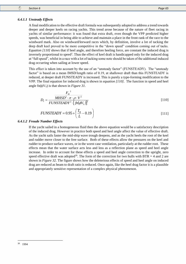
Section 6 Page 65
6.4.1.1 Unsteady Effects
A final modification to the effective draft formula was subsequently adopted to address a trend towards
deeper and deeper keels on racing yachts. This trend arose because of the nature of fleet racing in
yachts of similar performance: it was found that extra draft, even though the VPP predicted higher
speeds, was beneficial in being able to achieve and maintain a place in the front rank of the race to the
windward mark. Also on windward/leeward races which, by definition, involve a lot of tacking the
deep draft keel proved to be more competitive in the “down speed” condition coming out of tacks.
Equation [110] shows that if heel angle, and therefore heeling force, are constant the induced drag is
inversely proportional to speed2. Thus the effect of keel draft is handicapped only for the induced drag
at “full speed”, whilst in a race with a lot of tacking some note should be taken of the additional induced
drag occurring when sailing at lower speed.
This effect is taken into account by the use of an “unsteady factor” (FUNSTEADY). The “unsteady
factor” is based on a mean IMSD/length ratio of 0.19, at shallower draft than this FUNSTEADY is
reduced, at deeper draft FUNSTEADY is increased. This is purely a type-forming modification to the
VPP. The final equation for induced drag is shown in equation [110]. The function in speed and heel
angle fn(VS) is that shown in Figure 31.
22
22
2
S
H
IVfnFUNSTEADY
VMHSD
F
D
[110]
19.095.0
L
TFUNSTEADY R
[111]
6.4.1.2 Froude Number Effects
If the yacht sailed in a homogeneous fluid then the above equation would be a satisfactory description
of the induced drag. However in practice both speed and heel angle affect the value of effective draft.
As the yacht sails faster the mid-ship wave trough deepens, and as the yacht heels the root of the keel
and rudder move closer to the free surface. Both of these effects allow the pressures on the keel and
rudder to produce surface waves, or in the worst case ventilation, particularly at the rudder root. These
effects mean that the water surface acts less and less as a reflection plane as speed and heel angle
increase. In order to account for these effects a speed and heel angle correction to the upright, zero
speed effective draft was adopted39. The form of the correction for two hulls with BTR = 4 and 2 are
shown in Figure 32. The figure shows how the deleterious effects of speed and heel angle on induced
drag are reduced as beam to draft ratio is reduced. Once again, like the heel drag factor it is a plausible
and appropriately sensitive representation of a complex physical phenomenon.
39 1994
Section 6 Page 66
Figure 32 - Variation of effective draft with speed and heel angle
(Upper BTR = 4; Lower BTR =2)
6.4.1.3 Immersed transom
The following section describes a generic wave height calculation procedure for assessing the
immersed transom areas as a function of Froude Number and the calculation of the drag due to the
immersed transom The height of the wave at the end of the static WL was found from the wave
elevation observations of 13 non appended models of the Delft Systematic Series to be approximately
51
101 vlr
multWLend cLSM
VLRaWH [112]
where
5.1
3
11.2
cLSM
VOLcVLRmult
[113]
985.1log233.11 Fna [114]
Two different stern flow conditions are considered.
Variation of Effective Draft.
1.5
2.0
2.5
3.0
3.5
4.0
6.00 8.00 10.00 12.00 14.00 16.00
Speed (kts)
Eff
ec
tiv
e D
raft
(T
e)
(m)
0 deg Heel 17.5 deg. 25 deg. 30 deg.BTR=4
1.5
2.0
2.5
3.0
3.5
4.0
6 8 10 12 14 16
Speed (kts)
Eff
ec
tiv
e D
raft
(T
e)
(m)
BTR=2
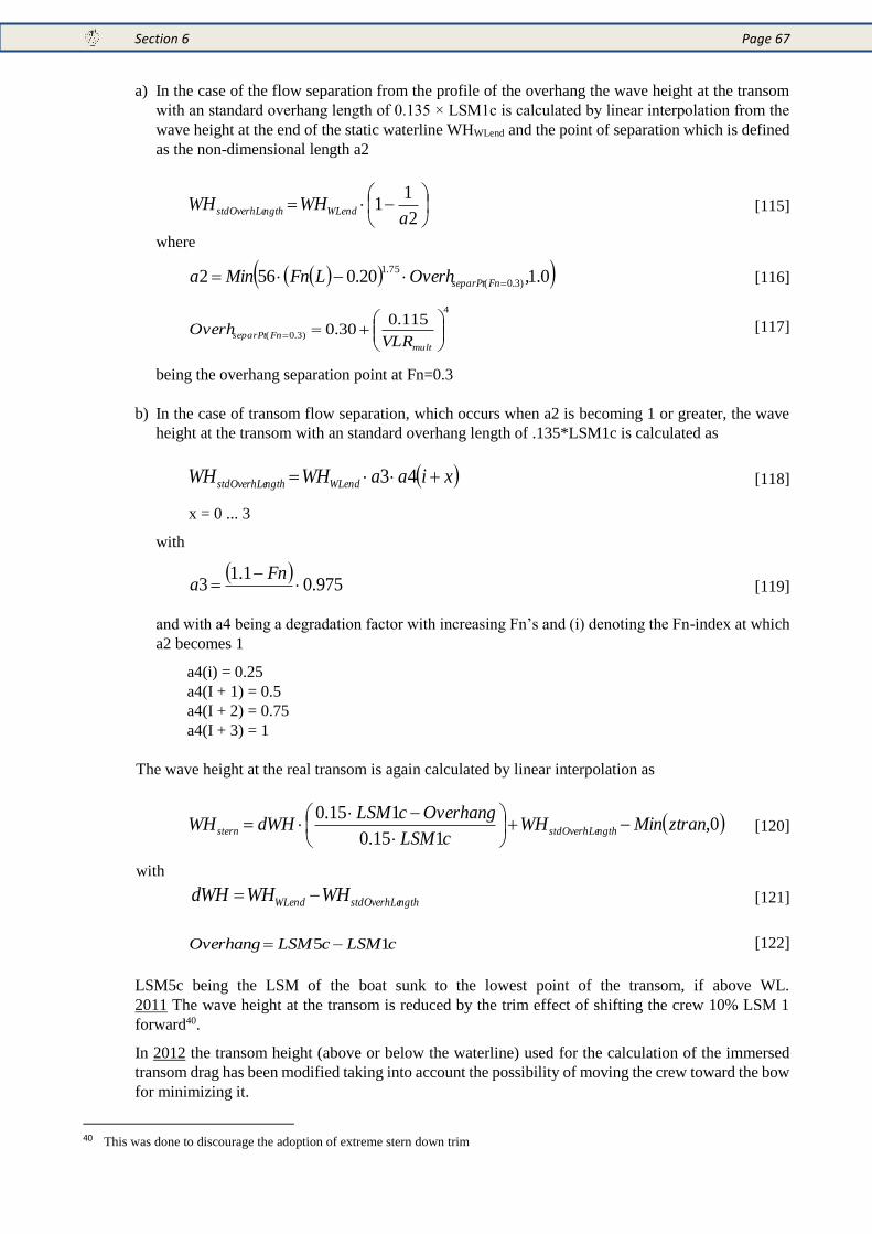
Section 6 Page 67
a) In the case of the flow separation from the profile of the overhang the wave height at the transom
with an standard overhang length of 0.135 × LSM1c is calculated by linear interpolation from the
wave height at the end of the static waterline WHWLend and the point of separation which is defined
as the non-dimensional length a2
2
11
aWHWH WLendngthstdOverhLe [115]
where
0.1,20.0562 )3.0(
75.1
FnseparPtOverhLFnMina [116]
4
)3.0(
115.030.0
mult
FnseparPtVLR
Overh [117]
being the overhang separation point at Fn=0.3
b) In the case of transom flow separation, which occurs when a2 is becoming 1 or greater, the wave
height at the transom with an standard overhang length of .135*LSM1c is calculated as
xiaaWHWH WLendngthstdOverhLe 43 [118]
x = 0 ... 3
with
975.01.1
3
Fn
a [119]
and with a4 being a degradation factor with increasing Fn’s and (i) denoting the Fn-index at which
a2 becomes 1
a4(i) = 0.25
a4(I + 1) = 0.5
a4(I + 2) = 0.75
a4(I + 3) = 1
The wave height at the real transom is again calculated by linear interpolation as
0,115.0
115.0ztranMinWH
cLSM
OverhangcLSMdWHWH ngthstdOverhLestern
[120]
with
ngthstdOverhLeWLend WHWHdWH [121]
cLSMcLSMOverhang 15 [122]
LSM5c being the LSM of the boat sunk to the lowest point of the transom, if above WL.
2011 The wave height at the transom is reduced by the trim effect of shifting the crew 10% LSM 1
forward40.
In 2012 the transom height (above or below the waterline) used for the calculation of the immersed
transom drag has been modified taking into account the possibility of moving the crew toward the bow
for minimizing it.
40 This was done to discourage the adoption of extreme stern down trim
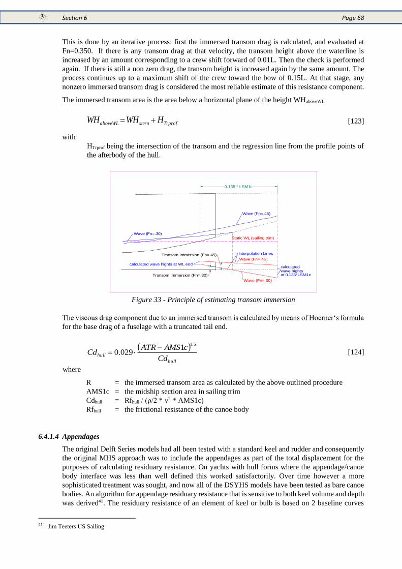
Section 6 Page 68
This is done by an iterative process: first the immersed transom drag is calculated, and evaluated at
Fn=0.350. If there is any transom drag at that velocity, the transom height above the waterline is
increased by an amount corresponding to a crew shift forward of 0.01L. Then the check is performed
again. If there is still a non zero drag, the transom height is increased again by the same amount. The
process continues up to a maximum shift of the crew toward the bow of 0.15L. At that stage, any
nonzero immersed transom drag is considered the most reliable estimate of this resistance component.
The immersed transom area is the area below a horizontal plane of the height WHaboveWL
TrprofsternaboveWL HWHWH [123]
with
HTrprof being the intersection of the transom and the regression line from the profile points of
the afterbody of the hull.
Figure 33 - Principle of estimating transom immersion
The viscous drag component due to an immersed transom is calculated by means of Hoerner‘s formula
for the base drag of a fuselage with a truncated tail end.
hull
hullCd
cAMSATRCd
5.11
029.0
[124]
where
R = the immersed transom area as calculated by the above outlined procedure
AMS1c = the midship section area in sailing trim
Cdhull = Rfhull / (ρ/2 * v2 * AMS1c)
Rfhull = the frictional resistance of the canoe body
6.4.1.4 Appendages
The original Delft Series models had all been tested with a standard keel and rudder and consequently
the original MHS approach was to include the appendages as part of the total displacement for the
purposes of calculating residuary resistance. On yachts with hull forms where the appendage/canoe
body interface was less than well defined this worked satisfactorily. Over time however a more
sophisticated treatment was sought, and now all of the DSYHS models have been tested as bare canoe
bodies. An algorithm for appendage residuary resistance that is sensitive to both keel volume and depth
was derived41. The residuary resistance of an element of keel or bulb is based on 2 baseline curves
41 Jim Teeters US Sailing
Static WL (sailing trim)Wave (Fn=.30)
Wave (Fn=.45)
Wave (Fn=.30)
Wave (Fn=.45)Transom Immersion (Fn=.45)
Transom Immersion (Fn=.30)
0.135 * LSM1c
calculatedwave hightsat 0.135*LSM1c
calculated wave hights at WL end
Interpolation Lines
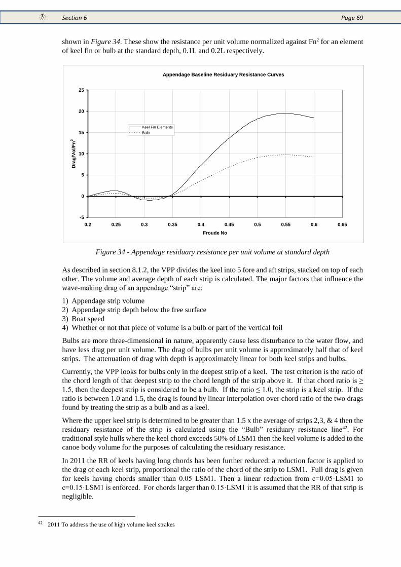
Section 6 Page 69
shown in Figure 34. These show the resistance per unit volume normalized against Fn2 for an element
of keel fin or bulb at the standard depth, 0.1L and 0.2L respectively.
Figure 34 - Appendage residuary resistance per unit volume at standard depth
As described in section 8.1.2, the VPP divides the keel into 5 fore and aft strips, stacked on top of each
other. The volume and average depth of each strip is calculated. The major factors that influence the
wave-making drag of an appendage “strip” are:
1) Appendage strip volume
2) Appendage strip depth below the free surface
3) Boat speed
4) Whether or not that piece of volume is a bulb or part of the vertical foil
Bulbs are more three-dimensional in nature, apparently cause less disturbance to the water flow, and
have less drag per unit volume. The drag of bulbs per unit volume is approximately half that of keel
strips. The attenuation of drag with depth is approximately linear for both keel strips and bulbs.
Currently, the VPP looks for bulbs only in the deepest strip of a keel. The test criterion is the ratio of
the chord length of that deepest strip to the chord length of the strip above it. If that chord ratio is ≥
1.5, then the deepest strip is considered to be a bulb. If the ratio ≤ 1.0, the strip is a keel strip. If the
ratio is between 1.0 and 1.5, the drag is found by linear interpolation over chord ratio of the two drags
found by treating the strip as a bulb and as a keel.
Where the upper keel strip is determined to be greater than 1.5 x the average of strips 2,3, & 4 then the
residuary resistance of the strip is calculated using the “Bulb” residuary resistance line42. For
traditional style hulls where the keel chord exceeds 50% of LSM1 then the keel volume is added to the
canoe body volume for the purposes of calculating the residuary resistance.
In 2011 the RR of keels having long chords has been further reduced: a reduction factor is applied to
the drag of each keel strip, proportional the ratio of the chord of the strip to LSM1. Full drag is given
for keels having chords smaller than 0.05 LSM1. Then a linear reduction from c=0.05·LSM1 to
c=0.15·LSM1 is enforced. For chords larger than 0.15·LSM1 it is assumed that the RR of that strip is
negligible.
42 2011 To address the use of high volume keel strakes
Appendage Baseline Residuary Resistance Curves
-5
0
5
10
15
20
25
0.2 0.25 0.3 0.35 0.4 0.45 0.5 0.55 0.6 0.65
Froude No
Dra
g/V
ol/
Fn
2
Keel Fin Elements
Bulb
Section 6 Page 70
AppendageCanoeRESIDUARY RrRrD [125]
6.4.2 Rail-under drag
Rail-under drag is not intended to calculate the drag of immersing the lee rail, it is an artifice intended
to prevent the VPP finding equilibrium sailing conditions at high heel angles. Rail-under drag is zero
up to a heel angle of 30 degrees. Above this value the upright residuary resistance is multiplied by a
factor and added to the total drag.
2300004.0 RESIDUARYDDRU [126]
6.5 Added Resistance in Waves, RAW
The addition of an added resistance in waves (RAW) module to the VPP43 was brought about by the fact
that cruising yachts, with outfitted interiors, were disadvantaged relative to their “stripped out” racing
rivals. This is not surprising, since reducing the yacht’s moment of inertia by concentrating weight
close to the centre of gravity will yield a performance gain when sailing in waves. The US Sailing
funded project to introduce this feature into the VPP had three aims which tackled the fundamentals
of predicting RAW:
1) Define a sea spectrum (wave energy density function) appropriate to the sailing venue
2) Devise a plausible and appropriately sensitive physical model of how parametric changes to the
yacht affect RAW when sailing in the sea state defined in 1
3) Devise a method by which a yacht’s pitch inertia could be determined directly by a physical test,
in the same way that stability is measured by an inclining test.
6.5.1 Wave Climate
As part of the research prior to introducing the RAW module, US Sailing funded the deployment of a
wave height measuring buoy at several popular sailing venues. The buoy was deployed during typical
races and the water surface elevations were recorded together with the wind speed. On the basis of
these measurements a single definition of wave climate was derived in the form of a wave energy
spectrum normalised for a true wind speed of one knot. This approach has the merit that it is relatively
easy to apply, because, whilst the significant height becomes a function of wind speed the modal period
remains fixed at 5 seconds.
Figure 35 - Wave energy as a function of True Wind Velocity
43 1990
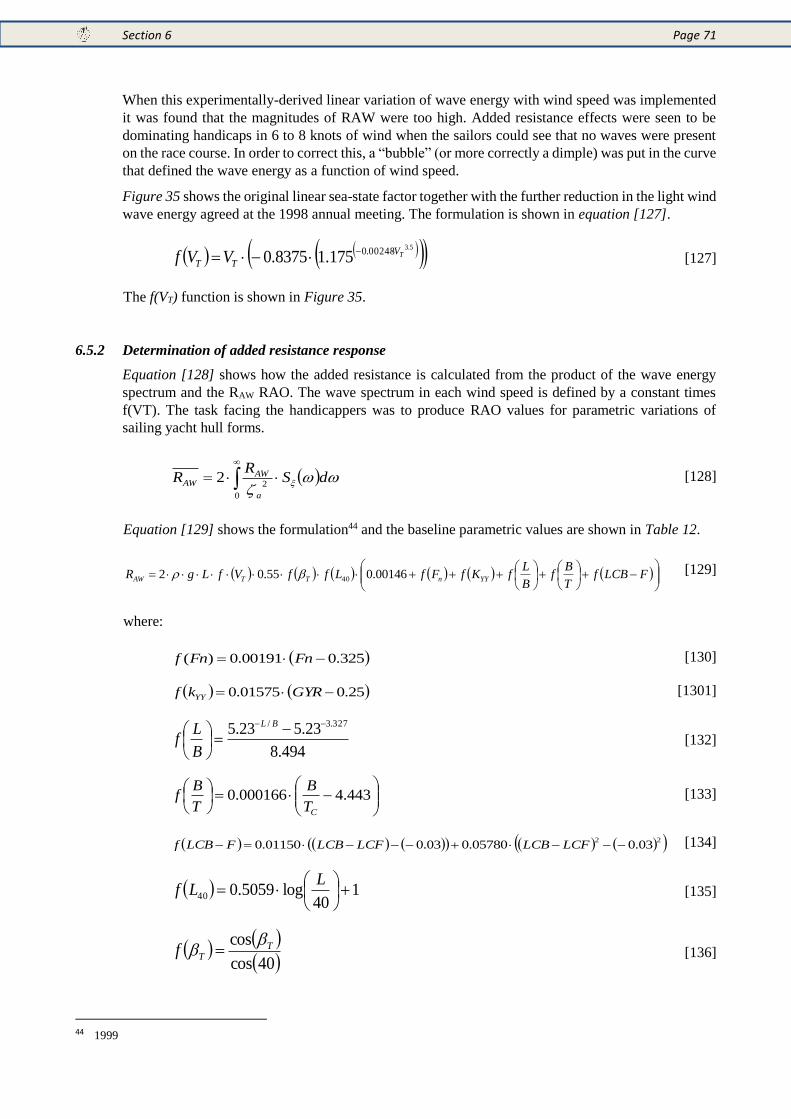
Section 6 Page 71
When this experimentally-derived linear variation of wave energy with wind speed was implemented
it was found that the magnitudes of RAW were too high. Added resistance effects were seen to be
dominating handicaps in 6 to 8 knots of wind when the sailors could see that no waves were present
on the race course. In order to correct this, a “bubble” (or more correctly a dimple) was put in the curve
that defined the wave energy as a function of wind speed.
Figure 35 shows the original linear sea-state factor together with the further reduction in the light wind
wave energy agreed at the 1998 annual meeting. The formulation is shown in equation [127].
5.300248.0
175.18375.0 TV
TT VVf
[127]
The f(VT) function is shown in Figure 35.
6.5.2 Determination of added resistance response
Equation [128] shows how the added resistance is calculated from the product of the wave energy
spectrum and the RAW RAO. The wave spectrum in each wind speed is defined by a constant times
f(VT). The task facing the handicappers was to produce RAO values for parametric variations of
sailing yacht hull forms.
0
22
dS
RR
a
AWAW
[128]
Equation [129] shows the formulation44 and the baseline parametric values are shown in Table 12.
FLCBf
T
Bf
B
LfKfFfLffVfLgR YYnTTAW 00146.055.02 40 [129]
where:
325.000191.0)( FnFnf [130]
25.001575.0 GYRkf YY [1301]
494.8
23.523.5 327.3/
BL
B
Lf [132]
443.4000166.0
CT
B
T
Bf [133]
2203.005780.003.001150.0 LCFLCBLCFLCBFLCBf [134]
140
log5059.040
LLf [135]
40cos
cos TTf
[136]
44 1999
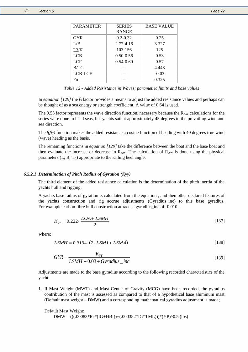
Section 6 Page 72
PARAMETER SERIES
RANGE
BASE VALUE
GYR 0.2-0.32 0.25
L/B 2.77-4.16 3.327
L3/ 103-156 125
LCB 0.50-0.56 0.53
LCF 0.54-0.60 0.57
B/TC -- 4.443
LCB-LCF -- -0.03
Fn -- 0.325
Table 12 - Added Resistance in Waves; parametric limits and base values
In equation [129] the fS factor provides a means to adjust the added resistance values and perhaps can
be thought of as a sea energy or strength coefficient. A value of 0.64 is used.
The 0.55 factor represents the wave direction function, necessary because the RAW calculations for the
series were done in head seas, but yachts sail at approximately 45 degrees to the prevailing wind and
sea direction.
The f(T) function makes the added resistance a cosine function of heading with 40 degrees true wind
(wave) heading as the basis.
The remaining functions in equation [129] take the difference between the boat and the base boat and
then evaluate the increase or decrease in RAW. The calculation of RAW is done using the physical
parameters (L, B, TC) appropriate to the sailing heel angle.
6.5.2.1 Determination of Pitch Radius of Gyration (Kyy)
The third element of the added resistance calculation is the determination of the pitch inertia of the
yachts hull and rigging.
A yachts base radius of gyration is calculated from the equation , and then other declared features of
the yachts construction and rig accrue adjustments (Gyradius_inc) to this base gyradius.
For example carbon fibre hull construction attracts a gyradius_inc of ‐0.010.
2
222.0LSMHLOA
KYY
[137]
where:
4123194.0 LSMLSMLSMH [138]
incGyradiusLSMH
KGYR YY
_03.0 [139]
Adjustments are made to the base gyradius according to the following recorded characteristics of the
yacht:
1. If Mast Weight (MWT) and Mast Center of Gravity (MCG) have been recorded, the gyradius
contribution of the mast is assessed as compared to that of a hypothetical base aluminum mast
(Default mast weight – DMW) and a corresponding mathematical gyradius adjustment is made;
Default Mast Weight:
DMW = (((.00083*IG*(IG+HBI))+(.000382*IG*TML)))*(YP)^0.5 (lbs)
Section 6 Page 73
Default Mast VCG:
DMVCG = 0.415*(IG+P+BAS)/2 –BAS (ft) above BAS
Default Rigging Weight:
DRW = LRW+JRW (lbs)
Default Rigging VCG:
DRVCG = (0.372*IG*LRW+0.5*(P+BAS+0.85*IG)*JRW)/DRW – BAS (ft) above BAS.
Default Mast+Rigging Weight:
DMW+DRW (lbs)
Default Mast+Rigging VCG above BAS:
(DMW*DMVCG+DRW*DRVCG)/(DMW+DRW) (ft).
where:
LRW (Lower Rigging Weight) = 0.000155*IG*YP (lbs)
JRW (Jumpers Rigging Weight) = 0.000027*(P+BAS-0.85*IG)*YP (lbs) (0 for masthead)
YP = (((RM25 * 25) + CARM * CW * cos(25°)) / (CP/2))
TML (Top Mast Length) = 0 on masthead and P + BAS – IG on fractional
RM25 = Righting Moment per degree at 25° heel
CARM = Crew Righting Arm
CW = Crew Weight
CP = Calculated Chainplate Width : Max(0.46 * J, 0.135 * IG)
“Masthead” is defined as an IG >= 0.95*(P + BAS).
2. For aestoma yacht with a carbon mast, where MWT and MCG are not recorded, the base gyradius
shall be adjusted taking as mast weight:
MWT = DMW *SQRT (70000/170000)
The mast weight for carbon mast is decreased of the square root of the ratio of the Young Modulus
of aluminum (70000 Mpa) and that of a very high modulus carbon mast (170000 Mpa) If the boat
is fitted with fiber rigging (PBO, carbon or similar) the rigging weight will be taken as: Rigging
Weight = 0.2 * DRW, being 20% of a conventional normal rod rig the weight of a aggressive fiber
weight.
3. Where MWT and MCG are not recorded, the number of spreader sets (including jumpers –one or
zero), adjustable inner forestays and running backstays (see 810.2I) are totaled. Gyradius is
increased by 0.002*CANOEL multiplied times the number by which the above total is less than 6.
This total is not taken less than zero;
4. If a yacht has a mizzen mast, Gyradius is increased by 0.002*CANOEL.
5. An adjustment is made for the classification of hull construction as follows:
SOLID: 0.016*CANOEL is added to Gyradius
CORED: 0.008*CANOEL is added
LIGHT: No adjustment
CARBON: 0.005*CANOEL is subtracted
CARBON FOR C/R 0.010*CANOEL is subtracted
HONEYCOMB: 0.006*CANOEL is subtracted where applicable in addition to adjustments
listed above;
6. For each year the yacht’s Age Date is less than 1989, 0.002*CANOEL is added to Gyradius, with
a maximum addition of credit for 8 years (an Age Date prior to 1981 is taken as 1981).
7. If the yacht has Forward Accommodation, FWD ADJ = 0.004 (see 11 below);
Section 6 Page 74
8. If the yacht’s rudder construction is carbon fiber, 0.003*CANOEL is subtracted from Gyradius;
9. If the yacht is in the cruiser/racer division and complies with IMS Appendix 1, C/R ADJ = 0.006
(see 10 below);
10. Any FWD ADJ (7 above) and any C/R ADJ (10 above) shall be added together and the sum reduced
according to an indicator of performance potential, i.e., sail area /volume ratio. The resulting
Accommodation Gyradius Increment is calculated as follows:
ACC GYR INCR = (C/R ADJ + FWD ADJ) * ((0.6763 * L + 19.6926 – SA/VOL)/(0.2263*
L + 2.6926)).The term multiplying (C/R ADJ + FWD ADJ) shall be neither negative nor
greater than 1.0.
SA/VOL = (AREA MAIN + AREA GENOA) / (DSPS/1025)2/3.
ACC GYR INCR * CANOEL is added to Gyradius.
11. If there is light material such as titanium or carbon used in lifeline elements (stanchions, pulpits,
pushpits, etc.) the gyrad_inc_fraction_of_L is decreased by 0.005
6.5.2.2 Cruiser/Racer pitch gyradius allowance scheme
This credit scheme is intended to allow for the greater pitching inertia of boats that race with anchor
and chain in the bow (anchor and chain should be located in the forward 30% of the boat and should
be lodged in forepeak fully reachable from deck.
The total gyradius increment due to the anchor and chain shall not be taken as more than
0.013*CANOEL. The gyradius increment will be added to the gyradius derived in.
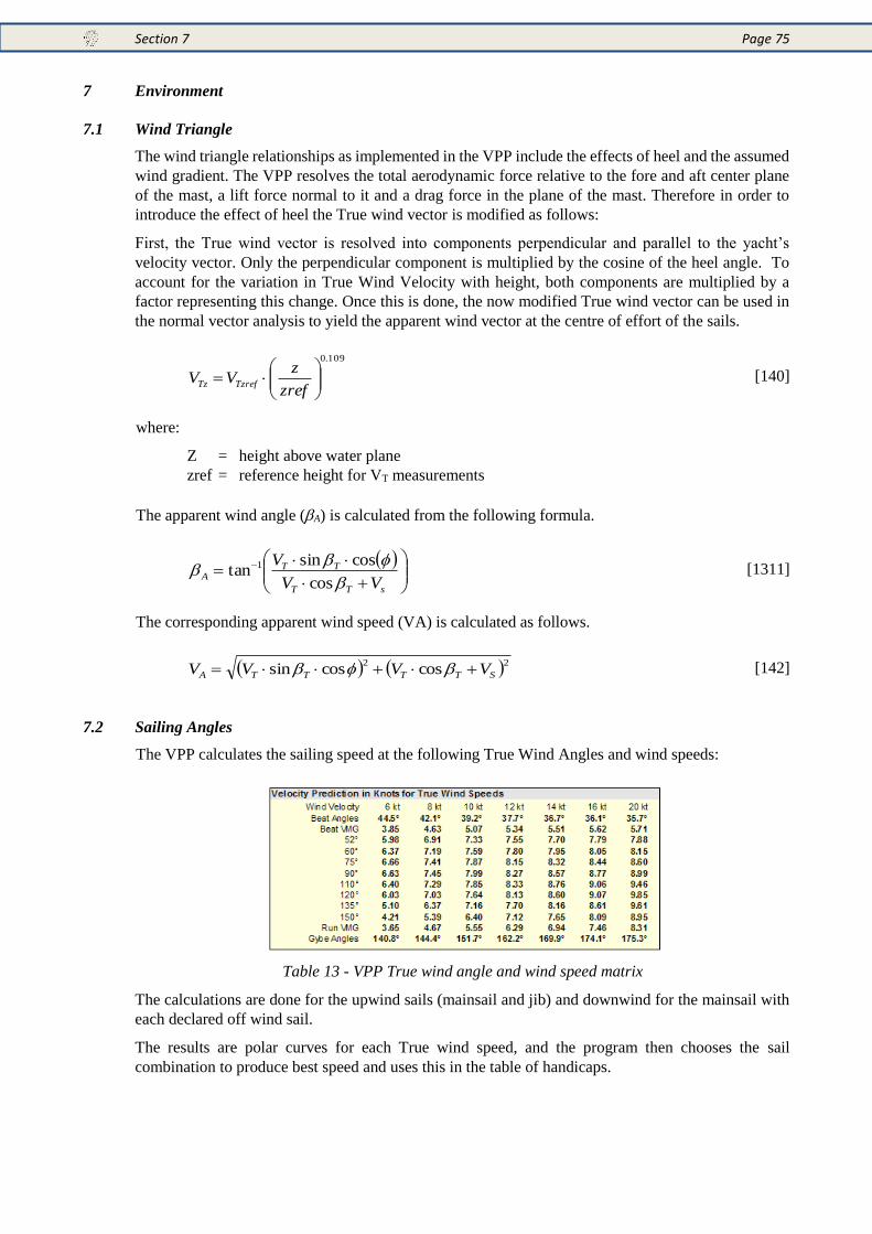
Section 7 Page 75
7 Environment
7.1 Wind Triangle
The wind triangle relationships as implemented in the VPP include the effects of heel and the assumed
wind gradient. The VPP resolves the total aerodynamic force relative to the fore and aft center plane
of the mast, a lift force normal to it and a drag force in the plane of the mast. Therefore in order to
introduce the effect of heel the True wind vector is modified as follows:
First, the True wind vector is resolved into components perpendicular and parallel to the yacht’s
velocity vector. Only the perpendicular component is multiplied by the cosine of the heel angle. To
account for the variation in True Wind Velocity with height, both components are multiplied by a
factor representing this change. Once this is done, the now modified True wind vector can be used in
the normal vector analysis to yield the apparent wind vector at the centre of effort of the sails.
109.0
zref
zVV TzrefTz
[140]
where:
Z = height above water plane
zref = reference height for VT measurements
The apparent wind angle (A) is calculated from the following formula.
sTT
TTA
VV
V
cos
cossintan 1 [1311]
The corresponding apparent wind speed (VA) is calculated as follows.
22coscossin STTTTA VVVV [142]
7.2 Sailing Angles
The VPP calculates the sailing speed at the following True Wind Angles and wind speeds:
Table 13 - VPP True wind angle and wind speed matrix
The calculations are done for the upwind sails (mainsail and jib) and downwind for the mainsail with
each declared off wind sail.
The results are polar curves for each True wind speed, and the program then chooses the sail
combination to produce best speed and uses this in the table of handicaps.

Section 7 Page 76
7.2.1 Velocity Made along the Course. (VMC)45
The VMC concept is similar to the VMG for upwind or downwind sailing. The goal is to reach the
mark, which is at an hypothetical prescribed heading, in the minimum time. This is accomplished
sometimes by a course different from the straight, shortest one. Sometimes a course made of two legs,
one closer to the wind and the other farther from it, is faster than the direct one. The implementation
of this concept is made by calculating the best VMC for the (TWS, TWA) printed in the certificate,
but using a splined continuous polar of the best performance of the boat evaluated at two degree
intervals.
45 2011
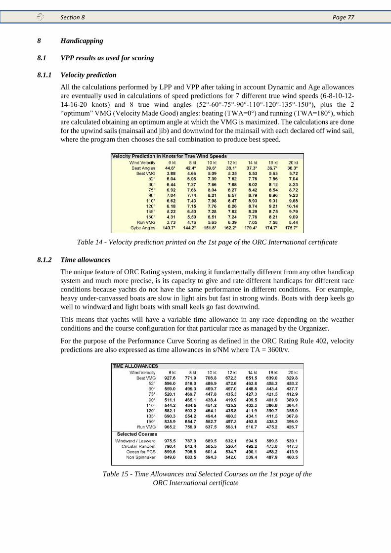
Section 8 Page 77
8 Handicapping
8.1 VPP results as used for scoring
8.1.1 Velocity prediction
All the calculations performed by LPP and VPP after taking in account Dynamic and Age allowances
are eventually used in calculations of speed predictions for 7 different true wind speeds (6-8-10-12-
14-16-20 knots) and 8 true wind angles (52°-60°-75°-90°-110°-120°-135°-150°), plus the 2
“optimum” VMG (Velocity Made Good) angles: beating (TWA=0°) and running (TWA=180°), which
are calculated obtaining an optimum angle at which the VMG is maximized. The calculations are done
for the upwind sails (mainsail and jib) and downwind for the mainsail with each declared off wind sail,
where the program then chooses the sail combination to produce best speed.
Table 14 - Velocity prediction printed on the 1st page of the ORC International certificate
8.1.2 Time allowances
The unique feature of ORC Rating system, making it fundamentally different from any other handicap
system and much more precise, is its capacity to give and rate different handicaps for different race
conditions because yachts do not have the same performance in different conditions. For example,
heavy under-canvassed boats are slow in light airs but fast in strong winds. Boats with deep keels go
well to windward and light boats with small keels go fast downwind.
This means that yachts will have a variable time allowance in any race depending on the weather
conditions and the course configuration for that particular race as managed by the Organizer.
For the purpose of the Performance Curve Scoring as defined in the ORC Rating Rule 402, velocity
predictions are also expressed as time allowances in s/NM where TA = 3600/v.
Table 15 - Time Allowances and Selected Courses on the 1st page of the
ORC International certificate
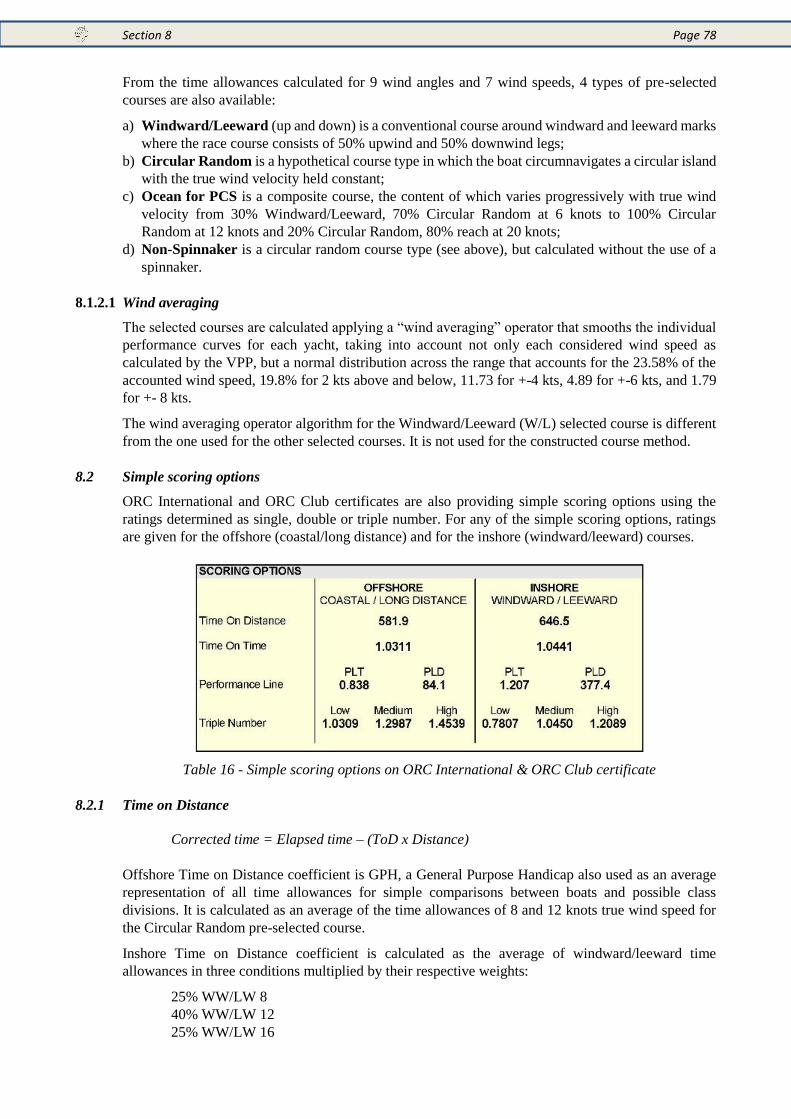
Section 8 Page 78
From the time allowances calculated for 9 wind angles and 7 wind speeds, 4 types of pre-selected
courses are also available:
a) Windward/Leeward (up and down) is a conventional course around windward and leeward marks
where the race course consists of 50% upwind and 50% downwind legs;
b) Circular Random is a hypothetical course type in which the boat circumnavigates a circular island
with the true wind velocity held constant;
c) Ocean for PCS is a composite course, the content of which varies progressively with true wind
velocity from 30% Windward/Leeward, 70% Circular Random at 6 knots to 100% Circular
Random at 12 knots and 20% Circular Random, 80% reach at 20 knots;
d) Non-Spinnaker is a circular random course type (see above), but calculated without the use of a
spinnaker.
8.1.2.1 Wind averaging
The selected courses are calculated applying a “wind averaging” operator that smooths the individual
performance curves for each yacht, taking into account not only each considered wind speed as
calculated by the VPP, but a normal distribution across the range that accounts for the 23.58% of the
accounted wind speed, 19.8% for 2 kts above and below, 11.73 for +-4 kts, 4.89 for +-6 kts, and 1.79
for +- 8 kts.
The wind averaging operator algorithm for the Windward/Leeward (W/L) selected course is different
from the one used for the other selected courses. It is not used for the constructed course method.
8.2 Simple scoring options
ORC International and ORC Club certificates are also providing simple scoring options using the
ratings determined as single, double or triple number. For any of the simple scoring options, ratings
are given for the offshore (coastal/long distance) and for the inshore (windward/leeward) courses.
Table 16 - Simple scoring options on ORC International & ORC Club certificate
8.2.1 Time on Distance
Corrected time = Elapsed time – (ToD x Distance)
Offshore Time on Distance coefficient is GPH, a General Purpose Handicap also used as an average
representation of all time allowances for simple comparisons between boats and possible class
divisions. It is calculated as an average of the time allowances of 8 and 12 knots true wind speed for
the Circular Random pre-selected course.
Inshore Time on Distance coefficient is calculated as the average of windward/leeward time
allowances in three conditions multiplied by their respective weights:
25% WW/LW 8
40% WW/LW 12
25% WW/LW 16
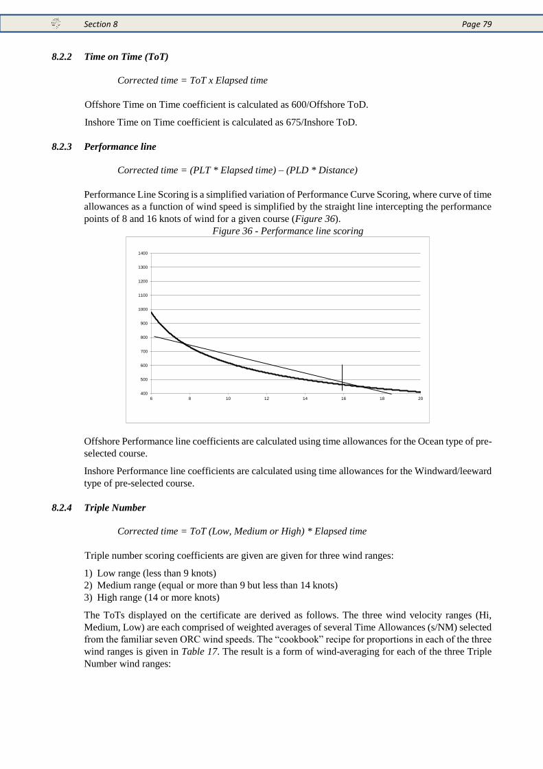
Section 8 Page 79
8.2.2 Time on Time (ToT)
Corrected time = ToT x Elapsed time
Offshore Time on Time coefficient is calculated as 600/Offshore ToD.
Inshore Time on Time coefficient is calculated as 675/Inshore ToD.
8.2.3 Performance line
Corrected time = (PLT * Elapsed time) – (PLD * Distance)
Performance Line Scoring is a simplified variation of Performance Curve Scoring, where curve of time
allowances as a function of wind speed is simplified by the straight line intercepting the performance
points of 8 and 16 knots of wind for a given course (Figure 36).
Figure 36 - Performance line scoring
Offshore Performance line coefficients are calculated using time allowances for the Ocean type of pre-
selected course.
Inshore Performance line coefficients are calculated using time allowances for the Windward/leeward
type of pre-selected course.
8.2.4 Triple Number
Corrected time = ToT (Low, Medium or High) * Elapsed time
Triple number scoring coefficients are given are given for three wind ranges:
1) Low range (less than 9 knots)
2) Medium range (equal or more than 9 but less than 14 knots)
3) High range (14 or more knots)
The ToTs displayed on the certificate are derived as follows. The three wind velocity ranges (Hi,
Medium, Low) are each comprised of weighted averages of several Time Allowances (s/NM) selected
from the familiar seven ORC wind speeds. The “cookbook” recipe for proportions in each of the three
wind ranges is given in Table 17. The result is a form of wind-averaging for each of the three Triple
Number wind ranges:
400
500
600
700
800
900
1000
1100
1200
1300
1400
6 8 10 12 14 16 18 20
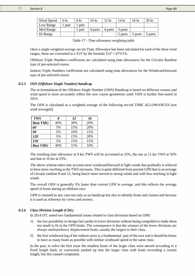
Section 8 Page 80
Wind Speed: 6 kt 8 kt 10 kt 12 kt 14 kt 16 kt 20 kt
Low Range 1 part 1 part
Med Range 1 part 4 parts 4 parts 3 parts
Hi Range 2 parts 3 parts 3 parts
Table 17 - Time allowance weighting table
Once a single weighted average sec/mi Time Allowance has been calculated for each of the three wind
ranges, these are converted to a ToT by the formula ToT = 675/TA.
Offshore Triple Numbers coefficients are calculated using time allowances for the Circular Random
type of pre-selected course.
Inshore Triple Numbers coefficients are calculated using time allowances for the Windward/leeward
type of pre-selected course.
8.2.5 OSN (Offshore Single Number) handicap
The re-formulation of the Offshore Single Number (OSN) Handicap is based on different courses and
wind speed to more accurately reflect the race course geometries used. OSN is further fine-tuned in
2014.
The OSN is calculated as a weighted average of the following sec/ml TIME ALLOWANCES (not
wind averaged):
TWS 8 12 16
Beat VMG 40% 30% 20%
60 5% 15% 20%
90 5% 10% 15%
120 5% 15% 20%
150 5% 15% 15%
Run VMG 40% 15% 10%
The resulting time allowance at 8 kts TWS will be accounted at 25%, the one at 12 kts TWS at 50%
and that at 16 kts at 25%.
The above scheme takes into account more windward/leeward in light winds that gradually is reduced
to have more reaching as the TWS increases. This is quite different from present GPH that is an average
of circular random 8 and 12, being hence more moved to strong winds and with less reaching in light
winds.
The overall OSN is generally 5% faster than current GPH in average, and this reflects the average
speed of boats during an offshore race.
GPH is retained in any case not only as an handicap but also to identify boats and classes and because
it is used as reference by crews and owners.
8.2.6 Class Division Length (CDL)
In 2014 ITC noted two fundamental issues related to class divisions based on GPH:
1) the low possibility to design fast yachts in lower divisions without being compelled to make them
too small to fit in the GPH limits. The consequence is that the winners of the lower divisions are
always medium/heavy displacement boats, usually the largest in their class.
2) the first windward leg of the inshore races is a fundamental part of the race and it should be better
to have as many boats as possible with similar windward speed in the same class.
In the past, to solve the first issue the smallest boats of the larger class were moved according to a
fixed length limit, or conversely pushed up into the larger class with boats exceeding a certain
length, but this caused complaints.
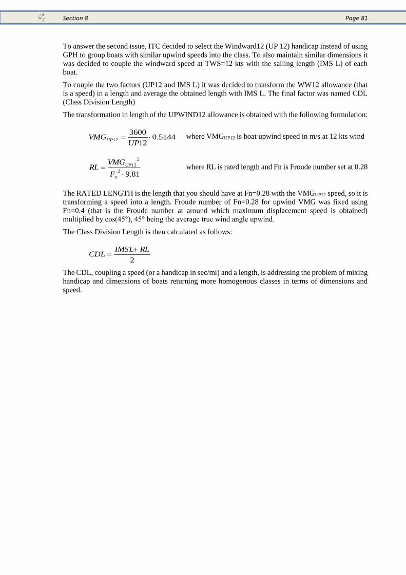
Section 8 Page 81
To answer the second issue, ITC decided to select the Windward12 (UP 12) handicap instead of using
GPH to group boats with similar upwind speeds into the class. To also maintain similar dimensions it
was decided to couple the windward speed at TWS=12 kts with the sailing length (IMS L) of each
boat.
To couple the two factors (UP12 and IMS L) it was decided to transform the WW12 allowance (that
is a speed) in a length and average the obtained length with IMS L. The final factor was named CDL
(Class Division Length)
The transformation in length of the UPWIND12 allowance is obtained with the following formulation:
5144.012
360012
UPVMGUP
where VMGUP12 is boat upwind speed in m/s at 12 kts wind
81.9
2
2
12
n
UP
F
VMGRL where RL is rated length and Fn is Froude number set at 0.28
The RATED LENGTH is the length that you should have at Fn=0.28 with the VMGUP12 speed, so it is
transforming a speed into a length. Froude number of Fn=0.28 for upwind VMG was fixed using
Fn=0.4 (that is the Froude number at around which maximum displacement speed is obtained)
multiplied by cos(45°), 45° being the average true wind angle upwind.
The Class Division Length is then calculated as follows:
2
RLLIMSCDL
The CDL, coupling a speed (or a handicap in sec/mi) and a length, is addressing the problem of mixing
handicap and dimensions of boats returning more homogenous classes in terms of dimensions and
speed.
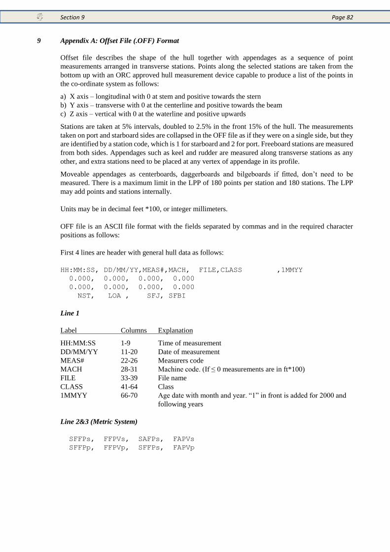
Section 9 Page 82
9 Appendix A: Offset File (.OFF) Format
Offset file describes the shape of the hull together with appendages as a sequence of point
measurements arranged in transverse stations. Points along the selected stations are taken from the
bottom up with an ORC approved hull measurement device capable to produce a list of the points in
the co-ordinate system as follows:
a) X axis – longitudinal with 0 at stem and positive towards the stern
b) Y axis – transverse with 0 at the centerline and positive towards the beam
c) Z axis – vertical with 0 at the waterline and positive upwards
Stations are taken at 5% intervals, doubled to 2.5% in the front 15% of the hull. The measurements
taken on port and starboard sides are collapsed in the OFF file as if they were on a single side, but they
are identified by a station code, which is 1 for starboard and 2 for port. Freeboard stations are measured
from both sides. Appendages such as keel and rudder are measured along transverse stations as any
other, and extra stations need to be placed at any vertex of appendage in its profile.
Moveable appendages as centerboards, daggerboards and bilgeboards if fitted, don’t need to be
measured. There is a maximum limit in the LPP of 180 points per station and 180 stations. The LPP
may add points and stations internally.
Units may be in decimal feet *100, or integer millimeters.
OFF file is an ASCII file format with the fields separated by commas and in the required character
positions as follows:
First 4 lines are header with general hull data as follows:
HH:MM:SS, DD/MM/YY,MEAS#,MACH, FILE,CLASS ,1MMYY
0.000, 0.000, 0.000, 0.000
0.000, 0.000, 0.000, 0.000
NST, LOA , SFJ, SFBI
Line 1
Label Columns Explanation
HH:MM:SS 1-9 Time of measurement
DD/MM/YY 11-20 Date of measurement
MEAS# 22-26 Measurers code
MACH 28-31 Machine code. (If ≤ 0 measurements are in ft*100)
FILE 33-39 File name
CLASS 41-64 Class
1MMYY 66-70 Age date with month and year. “1” in front is added for 2000 and
following years
Line 2&3 (Metric System)
SFFPs, FFPVs, SAFPs, FAPVs
SFFPp, FFPVp, SFFPs, FAPVp
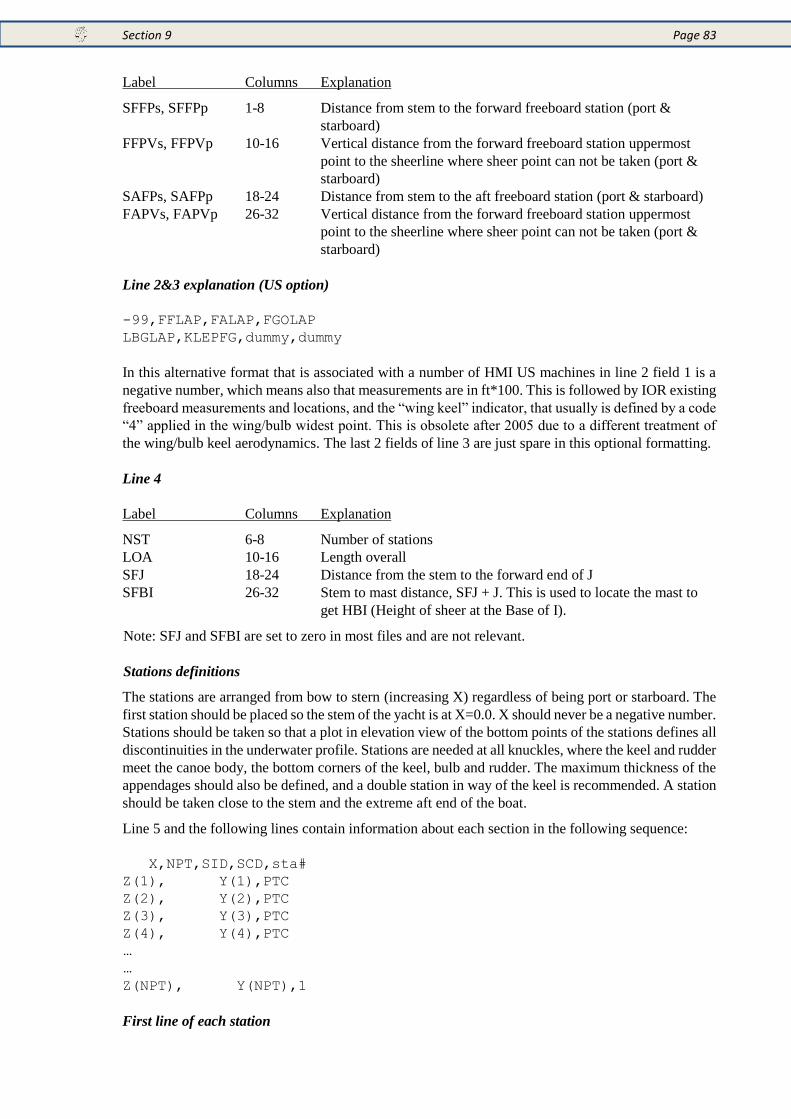
Section 9 Page 83
Label Columns Explanation
SFFPs, SFFPp 1-8 Distance from stem to the forward freeboard station (port &
starboard)
FFPVs, FFPVp 10-16 Vertical distance from the forward freeboard station uppermost
point to the sheerline where sheer point can not be taken (port &
starboard)
SAFPs, SAFPp 18-24 Distance from stem to the aft freeboard station (port & starboard)
FAPVs, FAPVp 26-32 Vertical distance from the forward freeboard station uppermost
point to the sheerline where sheer point can not be taken (port &
starboard)
Line 2&3 explanation (US option)
-99,FFLAP,FALAP,FGOLAP
LBGLAP,KLEPFG,dummy,dummy
In this alternative format that is associated with a number of HMI US machines in line 2 field 1 is a
negative number, which means also that measurements are in ft*100. This is followed by IOR existing
freeboard measurements and locations, and the “wing keel” indicator, that usually is defined by a code
“4” applied in the wing/bulb widest point. This is obsolete after 2005 due to a different treatment of
the wing/bulb keel aerodynamics. The last 2 fields of line 3 are just spare in this optional formatting.
Line 4
Label Columns Explanation
NST 6-8 Number of stations
LOA 10-16 Length overall
SFJ 18-24 Distance from the stem to the forward end of J
SFBI 26-32 Stem to mast distance, SFJ + J. This is used to locate the mast to
get HBI (Height of sheer at the Base of I).
Note: SFJ and SFBI are set to zero in most files and are not relevant.
Stations definitions
The stations are arranged from bow to stern (increasing X) regardless of being port or starboard. The
first station should be placed so the stem of the yacht is at X=0.0. X should never be a negative number.
Stations should be taken so that a plot in elevation view of the bottom points of the stations defines all
discontinuities in the underwater profile. Stations are needed at all knuckles, where the keel and rudder
meet the canoe body, the bottom corners of the keel, bulb and rudder. The maximum thickness of the
appendages should also be defined, and a double station in way of the keel is recommended. A station
should be taken close to the stem and the extreme aft end of the boat.
Line 5 and the following lines contain information about each section in the following sequence:
X,NPT,SID,SCD,sta#
Z(1), Y(1),PTC
Z(2), Y(2),PTC
Z(3), Y(3),PTC
Z(4), Y(4),PTC
…
…
Z(NPT), Y(NPT),1
First line of each station
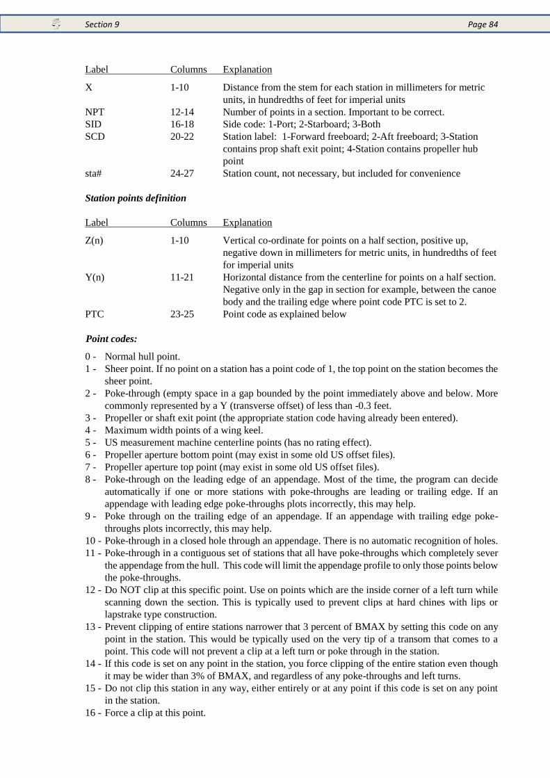
Section 9 Page 84
Label Columns Explanation
X 1-10 Distance from the stem for each station in millimeters for metric
units, in hundredths of feet for imperial units
NPT 12-14 Number of points in a section. Important to be correct.
SID 16-18 Side code: 1-Port; 2-Starboard; 3-Both
SCD 20-22 Station label: 1-Forward freeboard; 2-Aft freeboard; 3-Station
contains prop shaft exit point; 4-Station contains propeller hub
point
sta# 24-27 Station count, not necessary, but included for convenience
Station points definition
Label Columns Explanation
Z(n) 1-10 Vertical co-ordinate for points on a half section, positive up,
negative down in millimeters for metric units, in hundredths of feet
for imperial units
Y(n) 11-21 Horizontal distance from the centerline for points on a half section.
Negative only in the gap in section for example, between the canoe
body and the trailing edge where point code PTC is set to 2.
PTC 23-25 Point code as explained below
Point codes:
0 - Normal hull point.
1 - Sheer point. If no point on a station has a point code of 1, the top point on the station becomes the
sheer point.
2 - Poke-through (empty space in a gap bounded by the point immediately above and below. More
commonly represented by a Y (transverse offset) of less than -0.3 feet.
3 - Propeller or shaft exit point (the appropriate station code having already been entered).
4 - Maximum width points of a wing keel.
5 - US measurement machine centerline points (has no rating effect).
6 - Propeller aperture bottom point (may exist in some old US offset files).
7 - Propeller aperture top point (may exist in some old US offset files).
8 - Poke-through on the leading edge of an appendage. Most of the time, the program can decide
automatically if one or more stations with poke-throughs are leading or trailing edge. If an
appendage with leading edge poke-throughs plots incorrectly, this may help.
9 - Poke through on the trailing edge of an appendage. If an appendage with trailing edge poke-
throughs plots incorrectly, this may help.
10 - Poke-through in a closed hole through an appendage. There is no automatic recognition of holes.
11 - Poke-through in a contiguous set of stations that all have poke-throughs which completely sever
the appendage from the hull. This code will limit the appendage profile to only those points below
the poke-throughs.
12 - Do NOT clip at this specific point. Use on points which are the inside corner of a left turn while
scanning down the section. This is typically used to prevent clips at hard chines with lips or
lapstrake type construction.
13 - Prevent clipping of entire stations narrower that 3 percent of BMAX by setting this code on any
point in the station. This would be typically used on the very tip of a transom that comes to a
point. This code will not prevent a clip at a left turn or poke through in the station.
14 - If this code is set on any point in the station, you force clipping of the entire station even though
it may be wider than 3% of BMAX, and regardless of any poke-throughs and left turns.
15 - Do not clip this station in any way, either entirely or at any point if this code is set on any point
in the station.
16 - Force a clip at this point.
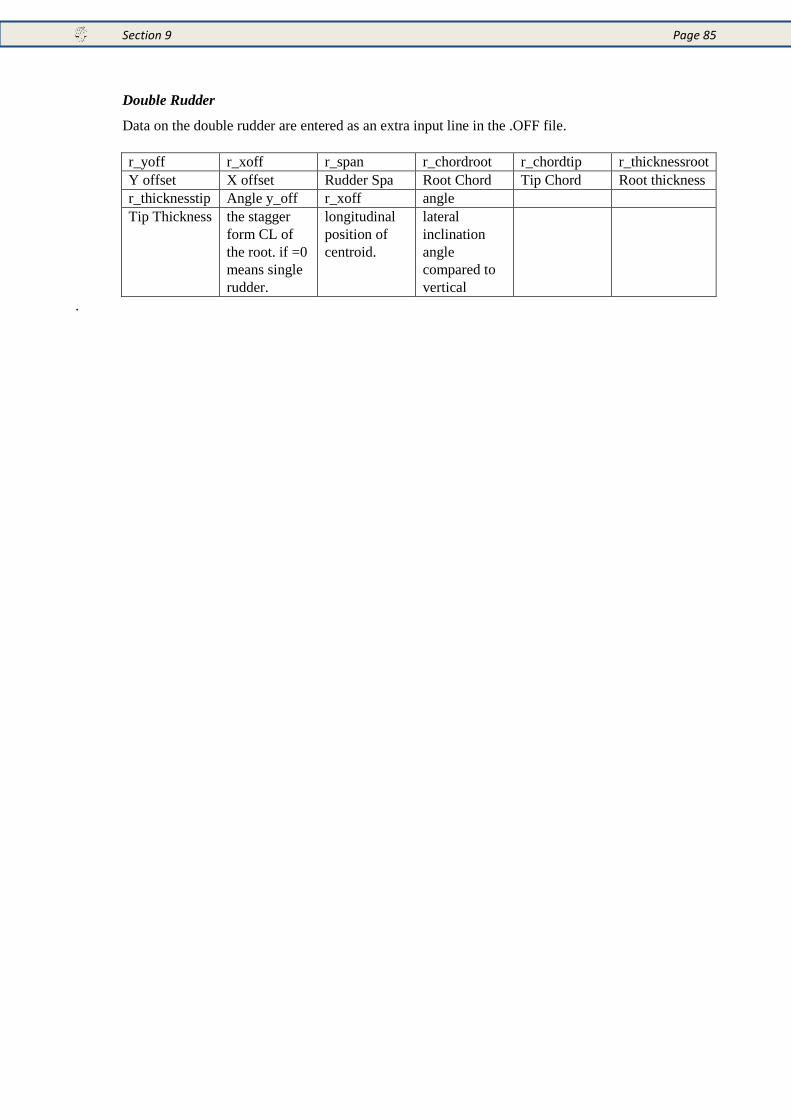
Section 9 Page 85
Double Rudder
Data on the double rudder are entered as an extra input line in the .OFF file.
r_yoff r_xoff r_span r_chordroot r_chordtip r_thicknessroot
Y offset X offset Rudder Spa Root Chord Tip Chord Root thickness
r_thicknesstip Angle y_off r_xoff angle
Tip Thickness the stagger
form CL of
the root. if =0
means single
rudder.
longitudinal
position of
centroid.
lateral
inclination
angle
compared to
vertical
.