ISSN: 1962-5361Disclaimer: This Philadelphia Fed working paper represents preliminary research that is being circulated for discussion purposes. The views expressed in these papers are solely those of the authors and do not necessarily reflect the views of the Federal Reserve Bank of Philadelphia or the Federal Reserve System. Any errors or omissions are the responsibility of the authors. Philadelphia Fed working papers are free to download at: https://philadelphiafed.org/research-and-data/publications/working-papers.

Working Papers

Vacancy Chains

Michael W.L. ElsbyUniversity of Edinburgh

Ryan MichaelsFederal Reserve Bank of Philadelphia Research Department

David RatnerBoard of Governors of the Federal Reserve System

WP 20-28July 2020https://doi.org/10.21799/frbp.wp.2020.28

1

VACANCY CHAINS

Michael W. L. Elsby Ryan Michaels David Ratner16F

*

July 2020

Preliminary and incomplete

Abstract

Replacement hiring—recruitment that seeks to replace positions vacated by workers who quit—plays a central role in establishment dynamics. We document this phenomenon using rich microdata on U.S. establishments, which frequently report no net change in their employment, often for years at a time, despite facing substantial gross turnover in the form of quits. We propose a model in which replacement hiring is driven by the presence of a putty-clay friction in the production structure of establishments. Replacement hiring induces a novel positive feedback channel through which an initial rise in vacancy posting induces still more vacancy posting to replace employees who are poached. This vacancy chain in turn induces volatile responses of vacancies, and thereby unemployment, to cyclical shocks. JEL codes: E32, J63, J64. Keywords: Quits, replacement hiring, unemployment, vacancies, business cycles.

* Elsby: University of Edinburgh (mike.elsby@ed.ac.uk). Michaels: Federal Reserve Bank of Philadelphia (ryan.michaels@phil.frb.org). Ratner: Federal Reserve Board (david.d.ratner@frb.gov). We thank Jess Helfand and Kathy Bauer and seminar participants at numerous institutions for helpful comments. We thank Trevor Dworetz for excellent research assistance. All errors are our own. This research was conducted with restricted access to Bureau of Labor Statistics (BLS) data. The views expressed here do not necessarily reflect the views of the BLS, the Federal Reserve Bank of Philadelphia, the staff and members of the Federal Reserve Board, or the Federal Reserve System as a whole. Elsby and Michaels gratefully acknowledge financial support from the UK Economic and Social Research Council (ESRC), Award reference ES/L009633/1.

2

What is a vacancy? After several decades of survey research dating back to the 1950s, the Bureau of Labor Statistics0F

1 converged on a definition of a vacancy that includes the notion that “a specific position exists and there is work available for that position.” This definition, implemented at the inception of the Job Openings and Labor Turnover Survey in December 2000, has in turn formed the basis of the leading source of vacancy data ever since, and become a central reference point for our understanding of the labor market response to the Great Recession.

In this paper, we argue that this definition of a vacancy also has rich economic implications. The notion of a “position” connotes the presence of some sunk investment: be it in physical capital—an empty desk, an unused machine—or organizational capital—the blueprint of task allocations at an establishment. The crucial implication that we explore is that this sunk capital—or “position”—remains even after an employee quits. We show that this observation has important implications for the volatility of labor market fluctuations at the macroeconomic level, and for the microeconomic foundations that give rise to this volatility.

We begin by documenting a novel set of stylized facts on establishments’ employment decisions using rich microdata from the Quarterly Census of Employment and Wages (QCEW) and the Job Openings and Labor Turnover Survey (JOLTS). These suggest a prominent role for replacement hiring—recruitment that replaces positions vacated by quits—in establishment dynamics. Establishments frequently report no net change in their employment, often for years at a time, despite facing substantial gross turnover in the form of quits. Furthermore, replacement hiring appears to account for a large fraction of aggregate hiring in the U.S. economy. Consistent with the BLS definition, the observation that establishments go to particular lengths to refill positions vacated by workers who quit further underscores a notion of a vacancy in which sunk investments loom large.

We then show that replacement hiring has potentially profound economic implications, both for the nature of labor market frictions as well as the volatility of labor market stocks and flows. In conventional models of labor market frictions the primary constraint to labor demand is the presence of a gross hiring cost (Mortensen and Pissarides 1994). By contrast, the prominence of replacement hiring suggests the presence of an alternative friction under which it is costly for firms to sustain net deviations from particular levels of employment.

A natural interpretation of this phenomenon that we pursue is that it has its origins in the production structure of firms. In particular, we explore the implications of a particular form of putty-clay technology that involves a reference level of employment that we refer to as “capacity.” Firms face a discrete marginal loss of output from operating below capacity. Capacity in turn can be adjusted only infrequently. The combination of these features

1 For further information on the evolution of these BLS surveys, see Elsby, Michaels and Ratner (2015).

3

induces a replacement hiring motive: Firms operating below capacity have particular incentives to hire.

To engage with the establishment-level stylized facts we document, we then embed this putty-clay production structure into a novel model of firm dynamics with on-the-job search. Firms with a decreasing returns putty-clay technology face idiosyncratic shocks that induce changes in their desired employment. The labor market is characterized by a hierarchy of firms, ranked by the surplus they can offer their workers. Given the opportunity, workers quit to firms with higher marginal surpluses. A consequence is that firms need to know the distribution of worker surpluses to infer their turnover, and thereby their optimal labor demand. In turn, this distribution is implied by the aggregate consequences of firms’ labor demand decisions. Labor market equilibrium thus involves the technical challenge of finding a fixed point for the distribution of worker surpluses. One of the contributions of this paper is that we are able solve for the steady-state labor market equilibrium of this environment.

The resultant properties of this steady-state equilibrium are illuminating and important. A distinctive consequence of the putty-clay technology we study, and the replacement hiring that it induces, is that it considerably alters the feedback of employment decisions across firms, and thereby the responses of aggregate vacancies and unemployment to changes in aggregate labor productivity. Conventional models of gross hiring costs capture a form of negative feedback across firms: Increased vacancy posting by other firms reduces vacancy-filling rates and raises quit rates. Both forces reduce the desired hiring of a given firm—it becomes more expensive to fill jobs, which in addition are less durable. As noted by Rogerson and Shimer (2010) this negative feedback moderates the responses of labor market outcomes in response to aggregate shocks.

Replacement hiring, by contrast, captures a novel positive feedback channel across firms: The rise in quits induced by increased vacancy posting by other firms now raises the desired hiring of a given firm, as it seeks to replace the positions vacated by quits. This positive feedback in turn raises the equilibrium responses of unemployment and vacancies. An initial rise in vacancy posting in an expansion induces still more vacancy posting to replace employees who are poached. This vacancy chain in turn induces a greater amplitude of responses of vacancies, and thereby unemployment, to changes in aggregate labor productivity. It is in this sense that the model has the potential to address the fundamental puzzle of why labor markets are so volatile, and the microeconomic origins that give rise to that volatility.

Motivated by this, we go on to explore the potential of the model on these dimensions quantitatively. The results are encouraging. The model is able to match many of the moments of replacement hiring that we document in establishment microdata. Notably, the model is able to match the persistence of inaction over net employment changes and generate a degree of replacement hiring that is a substantial share of aggregate hires. We then examine

4

the aggregate implications of replacement hiring by disciplining the model to these moments and examining the implied equilibrium responses of labor market stocks and flows to changes in aggregate productivity. The results suggest that the degree of replacement seen in the data induces significant positive feedback in vacancy creation. Strikingly, the implied amplitudes of unemployment, vacancies, job-finding rates, and job-loss rates closely resemble their empirical analogues.

As a point of contrast, we consider the implications of a version of the model that suspends the putty-clay aspect of the firms’ technology—that is, in which firms operate a conventional decreasing returns technology. By stark contrast, this version of the model is unable to match either the stylized facts of replacement hiring at the establishment level or the constellation of aggregate labor market responses. Viewed through the lens of the model, then, the putty-clay technology plays a key role in both accommodating the stylized facts of replacement hiring and generating plausible aggregate labor market responses.

Related literature. The view of the labor market set out in this paper dovetails with prior work along three themes. The first relates to the empirical literature on establishment dynamics pioneered in the early work of Davis and Haltiwanger (1992). More recently, Davis, Faberman and Haltiwanger (2012) have noted the importance of quits in driving a wedge between job flows and worker flows at the establishment level. Similarly, Burgess, Lane and Stevens (2001) document that both expanding and contracting employers experience a considerable “churn” of workers, a point echoed more recently by Lazear and Spletzer (2012). Our work further highlights the prominence of replacement hiring in establishments’ response to quits, and thereby the link between worker and job flows. More closely related to our empirical results is the work of Faberman and Nagypal (2008), who use JOLTS microdata to show that the incidence of quits at the establishment is often followed by vacancy posting and gross hiring, indicating the presence of replacement hiring. Our work presents a further array of evidence that reinforces the impression of pervasive replacement.

A second strand of related work is a recent stream of papers that have developed “large-firm” extensions of search and matching models that accommodate a notion of firm size (Acemoglu and Hawkins 2014; Elsby and Michaels 2013; Gavazza, Mongey and Violante 2016; Kaas and Kircher 2015). These have led to an enhanced understanding of the interaction between firm dynamics and unemployment, worker and job flows, and the aggregate dynamics of the labor market. Closer to our theoretical work, however, are a few recent papers that have begun to incorporate on-the-job search into these environments. As we noted, doing so raises a key challenge of solving for equilibrium distributions of worker surpluses. Fujita and Nakajima (2016) avoid this by assuming that workers have no bargaining power. Schaal (2017) avoids this by invoking directed search with firm

5

commitment. Closest to our approach is a set of papers that do address this challenge in models that integrate firm dynamics and on-the-job search. Lentz and Mortensen (2012) focus on the dispersion of steady-state productivity and wages. Bilal et al. (2019) study entry, exit, worker flows and employment dynamics over firm lifecycles. Elsby and Gottfries (2019) provide analytical characterizations of labor demand and the distributions of worker surpluses, and use them to simplify the solution of out-of-steady-state aggregate dynamics. Our key focus—the prominence of replacement hiring, its origins, and its aggregate implications—is not taken up in these works, however.1F

2 A third strand of related literature comprises work that explicitly incorporates a notion

of a vacancy chain. This concept has a rich heritage in quantitative sociology, pioneered in the early work of White (1970), with applications to topics as diverse as the turnover of shells among hermit crabs and of pastorates among Methodist ministers (Chase 1991). Within economics, the literature is much smaller. Akerlof, Rose and Yellen (1988) use the idea to explain the procyclicality of job-to-job quits, but in their model vacancy chains do not amplify labor market responses. Most related to our work is a recent paper by Schoefer (2019) that was conceived concurrently with the present paper. Schoefer presents evidence based on German microdata suggesting that increased quits induce increased hiring in the future, reminiscent of Faberman and Nagypal’s evidence based on JOLTS microdata for the U.S. and suggestive of replacement hiring. He then devises a simple extension of the textbook one-worker-firm Diamond, Mortensen and Pissarides model to accommodate long-lived jobs, and thereby replacement hiring. Because the evidence we use is drawn from establishment data, our model instead focuses on integrating firm dynamics, with replacement driven by a putty-clay technology. Reassuringly, both Schoefer’s model and ours share the prediction that replacement hiring-driven vacancy chains amplify labor market responses.

1. Data

We use restricted-access microdata from the Quarterly Census of Employment and Wages (QCEW) and the Job Openings and Labor Turnover Survey (JOLTS) for the United States. Both sources permit longitudinal linking of establishments over time, thereby allowing an analysis of establishment dynamics.

Quarterly Census of Employment and Wages. The QCEW covers approximately 98 percent of employees on non-farm payrolls in the United States and territories, and is a near-census of 2 Krause and Lubik (2006) study the effects of on-the-job search in a model with constant returns and find that it can generate realistic variation in labor market flows. This derives, in part, from the procyclicality of on-the-job search intensity in the model. Recent work by Mukoyama et al (2018), however, suggests weak evidence for cyclical search intensity, and so our analysis will treat the latter as fixed.

6

non-agricultural workers in private establishments. The data are collected by the Bureau of Labor Statistics (BLS) in concert with State Employment Security Agencies, which run state unemployment insurance (UI) programs and cover all employers with employees covered by UI. Each month, firms are required to submit a count of employees and a quarterly compensation bill, which the BLS aggregates to form the QCEW. The BLS then links establishments in the QCEW over time to create the Longitudinal Database of Establishments (LDE).

We have been granted access to QCEW/LDE microdata for a subset of forty states, including Washington, DC, but excluding Florida, Illinois, Massachusetts, Michigan, Mississippi, New Hampshire, New York, Oregon, Pennsylvania, Wisconsin, and Wyoming. These microdata permit longitudinal linking of establishments over time from the early 1990s through to the second quarter of 2014.

We further restrict our samples to privately owned establishments2F

3 and to continuing establishments with positive employment in consecutive quarters. Specifically, we construct a set of overlapping quarter-to-quarter balanced panels that exclude births and deaths of establishments within the quarter. Note that we do not balance across quarters, so births in a given panel will appear as incumbents in the subsequent panel (if they survive). This eliminates about 2 percent of establishments.3F

4 As an example of the sample sizes involved, in the second quarter of 2014 our samples cover about 5 million establishments and 77 million workers.

We use these samples to track quarterly net changes in establishment employment through time. The BLS defines monthly employment as the count of employees on an establishment’s payroll for the pay period encompassing the 12th of each month.4F

5 We follow BLS procedure by focusing on quarterly data and defining quarterly employment as employment in the third month of each quarter. Thus, the net employment change in, for example, the first quarter of a given year is the difference between employment in March of that year and in December of the previous year.

Job Openings and Labor Turnover Survey. The JOLTS data cover approximately 16,000 establishments per month. The sample is constructed from two subsamples: a certainty 3 We exclude establishments in public administration (NAICS industry 92) and those that are not in a classified industry (NAICS code 99). Excluding privately owned unclassified establishments eliminates approximately 225,000 employees (about 0.1 percent of total employment) in approximately 190,000 establishments (about 2 percent of total establishments) in the published, aggregate QCEW data. These restrictions are consistent with those imposed in prior literature on employment dynamics such as Foote (1998). 4 We also restrict attention to establishments that are not flagged as being a successor or predecessor of another establishment between quarters to be more confident in continuing establishment linkages. This accounts for approximately 0.1 percent of establishments in the second quarter of 2014. 5 The count of workers includes all those receiving any pay during the pay period, including part-time workers and those on paid leave.

7

panel of establishments that are always included, and a rotating panel of establishments that are sampled for 24 months. We use JOLTS microdata from December 2000 through the middle of 2016.

Crucially for our purposes, the JOLTS samples include rich data on gross worker turnover, measuring hires and separations, and their composition into quits and layoffs, at the establishment level. As in the QCEW, employment is measured for the pay period including the 12th of each month. Gross flows of workers in JOLTS are measured as flows that accrue over the course of a month. Hires are the total number of additions to the establishment’s payrolls.5F

6 Separations are split into three broad categories based on the reason for termination. Quits are defined as voluntary separations initiated by the employee (excluding retirements). Layoffs and discharges are defined as involuntary separations due to cause or business conditions. Other separations are defined to include retirements, transfers, deaths, or separations due to disability. Total separations are the sum of all three components.

We apply two adjustments to the raw JOLTS data. First, all empirical results are weighted using the sample weights provided by the BLS. Second, in cases where an establishment’s employment deviates from that implied by its hires and separations, we follow Davis, Faberman, and Haltiwanger (2013) and adjust an establishment’s employment to be consistent with reported gross flows.

2. Stylized facts on replacement hiring In this section, we use the establishment-level QCEW and JOLTS microdata described above to document a set of stylized facts on the interplay between establishment-level (net) employment adjustment and gross worker turnover. These suggest a prominent empirical role for replacement hiring. These facts will motivate the remainder of the paper, which sets out important ramifications of replacement hiring for the microfoundations of labor market frictions and the roots of aggregate labor market volatility.

2.1 Inaction over net employment changes Our first fact is illustrated in Figure 1, which plots the distribution of quarterly employment growth at the establishment level using both the QCEW and JOLTS microdata.6F

7 This reveals a long-recognized feature of establishment dynamics, namely that employment adjustment is marked by substantial inaction (Hamermesh 1989; Davis and Haltiwanger 1992). A large

6 These include both new hires and rehires, as well as part-time or full-time workers. 7 Each establishment’s growth rate, 𝑔𝑔𝑡𝑡 , is calculated as in Davis, Haltiwanger, and Schuh (1996), 𝑔𝑔𝑡𝑡 =(𝑛𝑛𝑡𝑡 − 𝑛𝑛𝑡𝑡−1)/[(𝑛𝑛𝑡𝑡 + 𝑛𝑛𝑡𝑡−1) 2⁄ ]. We then collect establishments' growth rates into bins of varying widths.

8

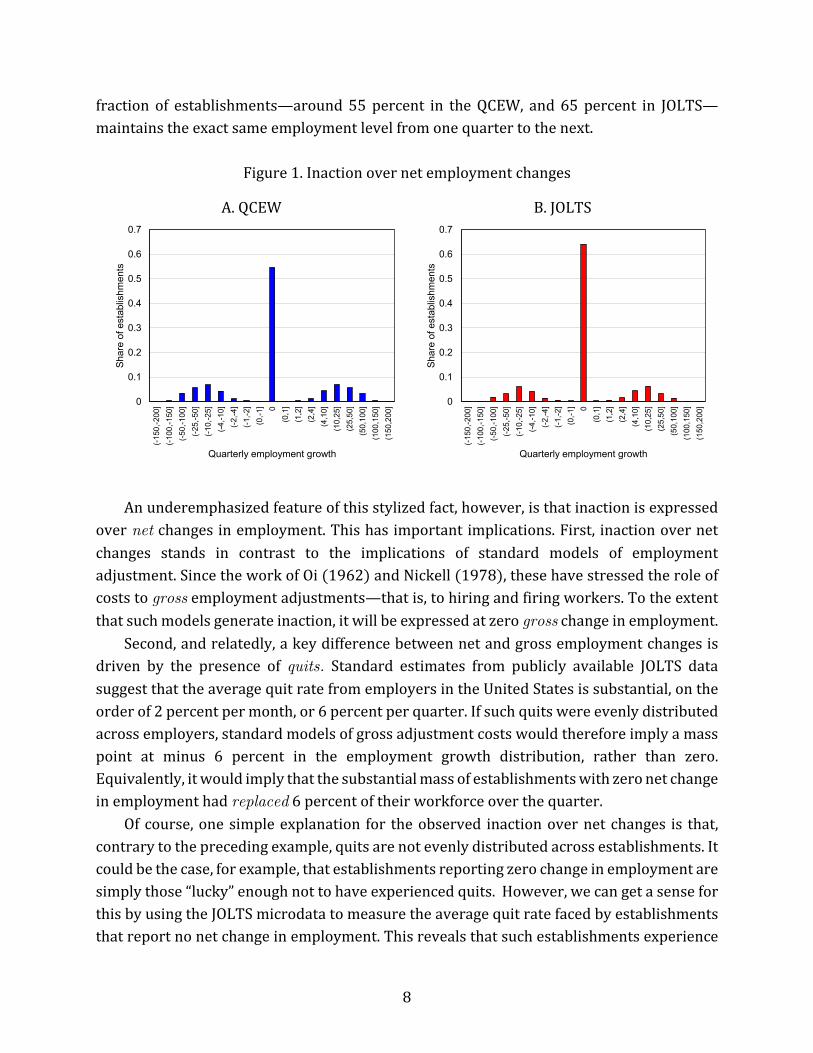
fraction of establishments—around 55 percent in the QCEW, and 65 percent in JOLTS—maintains the exact same employment level from one quarter to the next.

Figure 1. Inaction over net employment changes

A. QCEW B. JOLTS

An underemphasized feature of this stylized fact, however, is that inaction is expressed

over net changes in employment. This has important implications. First, inaction over net changes stands in contrast to the implications of standard models of employment adjustment. Since the work of Oi (1962) and Nickell (1978), these have stressed the role of costs to gross employment adjustments—that is, to hiring and firing workers. To the extent that such models generate inaction, it will be expressed at zero gross change in employment.

Second, and relatedly, a key difference between net and gross employment changes is driven by the presence of quits. Standard estimates from publicly available JOLTS data suggest that the average quit rate from employers in the United States is substantial, on the order of 2 percent per month, or 6 percent per quarter. If such quits were evenly distributed across employers, standard models of gross adjustment costs would therefore imply a mass point at minus 6 percent in the employment growth distribution, rather than zero. Equivalently, it would imply that the substantial mass of establishments with zero net change in employment had replaced 6 percent of their workforce over the quarter.

Of course, one simple explanation for the observed inaction over net changes is that, contrary to the preceding example, quits are not evenly distributed across establishments. It could be the case, for example, that establishments reporting zero change in employment are simply those “lucky” enough not to have experienced quits. However, we can get a sense for this by using the JOLTS microdata to measure the average quit rate faced by establishments that report no net change in employment. This reveals that such establishments experience

0

0.1

0.2

0.3

0.4

0.5

0.6

0.7

(-150

,-200

](-1

00,-1

50]

(-50,

-100

](-2

5,-5

0](-1

0,-2

5](-4

,-10]

(-2,-4

](-1

,-2]

(0,-1

] 0(0

,1]

(1,2

](2

,4]

(4,1

0](1

0,25

](2

5,50

](5

0,10

0](1

00,1

50]

(150

,200

]

Shar

e of

est

ablis

hmen

ts

Quarterly employment growth

0

0.1

0.2

0.3

0.4

0.5

0.6

0.7

(-150

,-200

](-1

00,-1

50]

(-50,

-100

](-2

5,-5

0](-1

0,-2

5](-4

,-10]

(-2,-4

](-1

,-2]

(0,-1

] 0(0

,1]

(1,2

](2

,4]

(4,1

0](1

0,25

](2

5,50

](5

0,10

0](1

00,1

50]

(150

,200

]

Shar

e of

est

ablis

hmen

ts

Quarterly employment growth

9

quit rates on the order of 3.2 percent per quarter—lower than average, but nonetheless substantial.

The combination of such nontrivial quit rates and observed inaction over net employment changes suggests that establishments frequently hire to replace exactly those workers that quit. We refer to this phenomenon as replacement hiring. In the remainder of this section, we explore several of its further implications.

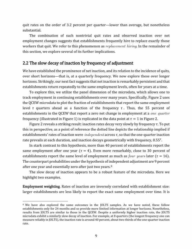
2.2 The slow decay of inaction by frequency of adjustment We have established the prominence of net inaction, and its relation to the incidence of quits, over short horizons—that is, at a quarterly frequency. We now explore these over longer horizons. Strikingly, our next fact suggests that net inaction is remarkably persistent and that establishments return repeatedly to the same employment levels, often for years at a time.

To explore this, we utilize the panel dimension of the microdata, which allows one to track employment in continuing establishments over many years. Specifically, Figure 2 uses the QCEW microdata to plot the fraction of establishments that report the same employment level 𝜏𝜏 quarters ahead as a function of the frequency 𝜏𝜏 . Thus, the 55 percent of establishments in the QCEW that report a zero net change in employment at a one quarter frequency (illustrated in Figure 1) is replicated in the data point at 𝜏𝜏 = 1 in Figure 2.

Figure 2 reveals a striking result: inaction rates decay very slowly by frequency 𝜏𝜏. To put this in perspective, as a point of reference the dotted line depicts the relationship implied if establishments’ rates of inaction were independent across 𝜏𝜏, so that the one-quarter inaction rate prevails at each duration, and inaction decays geometrically with frequency, 0.55𝜏𝜏.

In stark contrast to this hypothesis, more than 40 percent of establishments report the same employment after one year (𝜏𝜏 = 4). Even more remarkably, close to 30 percent of establishments report the same level of employment as much as four years later (𝜏𝜏 = 16). The counterpart probabilities under the hypothesis of independent adjustment are 9 percent after one year and essentially zero after just two years.7F

8 The slow decay of inaction appears to be a robust feature of the microdata. Here we

highlight two examples.

Employment weighting. Rates of inaction are inversely correlated with establishment size: larger establishments are less likely to report the exact same employment over time. It is

8 We have also explored the same outcomes in the JOLTS samples. As we have noted, these follow establishments only for 24 months and so provide more limited information at longer horizons. Nonetheless, results from JOLTS are similar to those in the QCEW. Despite a uniformly higher inaction rate, the JOLTS microdata exhibit a similarly slow decay of inaction. For example, at 8 quarters (the longest frequency one can measure reliably in JOLTS), the inaction rate is around 40 percent, about two-thirds of the one-quarter inaction rate.

10

natural to question whether the remarkable persistence of employment seen in the data is driven by small establishments.

Figure 2. The slow decay of inaction by frequency of adjustment (QCEW)

A. By weighting scheme / window B. By industry seasonality

To examine this possibility, Figure 2 reports establishment employment-weighted rates

of inaction by frequency. Although size-weighting does indeed reduce estimated rates of inaction, much of this reduction can be traced to small employment changes. For example, while employment weighting reduces the one-quarter inaction rate to just 16 percent, this rises again to 40 percent once one includes small employment changes of one worker, or one percent of the workforce. Widening the inaction window further to two workers, or two percent of the workforce, in turn raises estimated employment-weighted inaction rates back to the neighborhood of their establishment-weighted counterparts.

Importantly, the decay of estimated net inaction rates by frequency is only modestly more rapid after employment weighting. Four-year inaction probabilities are approximately 40 percent of their one-quarter counterparts for all of the inaction windows plotted in Figure 2.

Seasonality. An alternative hypothesis is that the slow decay of inaction is an artefact of seasonality, for example if an employer chooses not to replace quits after its high season but returns to its high-season workforce in subsequent years. Under this hypothesis the rate of decay should be particularly low in industries where a larger share of employment fluctuations are seasonal. Figure 2 slices the data into high-, medium- and low-seasonal

0.0

0.1

0.2

0.3

0.4

0.5

0.6

0.7

0 2 4 6 8 10 12 14 16

Prob

(em

p. a

t t=

emp.

at t

+τ)

Frequency τ in quarters

Estab. weightedEmpl. weighted… (+/- max{1,1%} )… (+/- max{2,2%} )

0.0

0.1

0.2

0.3

0.4

0.5

0.6

0.7

0 2 4 6 8 10 12 14 16Pr

ob (e

mp.

at t

= em

p. a

t t+τ)

Frequency τ in quarters

Low seasonality

Medium seasonality

High seasonality

11

industries by ranking the seasonal variances of their employment.8F

9 This reveals, however, that a similar pattern emerges across all seasonal categories—inaction is prevalent and slow to decay.

The striking persistence of the exact same establishment size suggests that employers have “reference” levels of employment to which they return routinely,9F

10 and do so via replacement hiring.

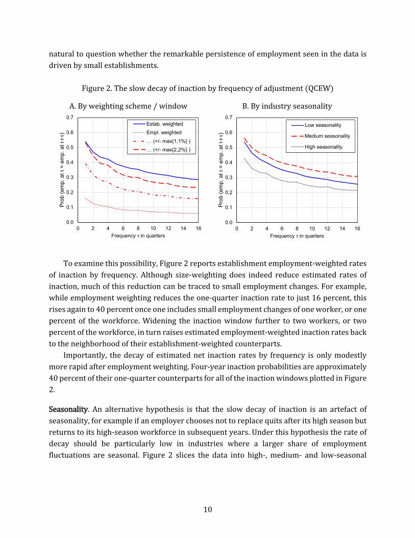
2.3 Cumulative gross turnover among inactive establishments Our third stylized fact returns to the question of how much gross turnover occurs at inactive establishments. We noted above that establishments that remain at the same employment level from one quarter to the next experience nontrivial quit rates, averaging more than 3 percent per quarter. We have also shown that net inaction is not merely prevalent at the one quarter frequency, but that establishments tend to maintain the same employment level for long periods, often years at a time. Here, we explore whether these establishments that remain inactive for long periods also experience substantial cumulative worker turnover and thereby get a sense of the magnitude of the intervening replacement hiring they implement to maintain their employment.

Specifically, in any given month of JOLTS microdata, we identify establishments that report the same employment level when surveyed 𝜏𝜏 months later. Among these establishments, we compute cumulative rates of worker turnover experienced by these establishments over the course of the intervening 𝜏𝜏 months. Recalling that establishments included in the rotating panel element of the JOLTS sample are followed for 24 months, we implement this method for 𝜏𝜏s between one and 24 months.

Figure 3 reports the results of this exercise, pooled over all available months of JOLTS microdata. This reiterates the high-frequency results cited in our earlier discussion of Figure 1: Establishments reporting the same employment quarter-to-quarter also report gross hires (and, by definition, separations) equal to 5 percent of their workforce, 3.2 percent of which have replaced workers that quit and another 0.4 percent of which are separations for other voluntary reasons.10F

11

9 We estimate seasonal variance by regressing publicly available monthly employment data from the QCEW at the three-digit industry level on month dummies and taking the variance of the estimated coefficients. We then rank industries from lowest to highest variance and define low-seasonal industries as the lowest quartile, and high-seasonal industries as the highest quartile, of these variances. Examples of low-seasonal industries are many health care industries, and an example of a high-seasonal industry is crop production. 10 This observation mirrors the evidence from price microdata for the presence of “reference” price levels (Eichenbaum, Jaimovich, and Rebelo 2011). 11 We focus on quits and other separations since those are likely to be involuntary from the perspective of the employer and would require replacement if the employer was looking to maintain a constant level of

12

Figure 3. Cumulative gross turnover among inactive establishments (JOLTS)

An important message of Figure 3, however, is that considerable gross worker turnover accumulates, almost linearly, in inactive establishments over longer frequencies. In particular, at a two-year horizon, over which nearly 40 percent of establishments report the same employment in the JOLTS microdata, gross hires in these establishments are replacing on average 35 percent of their workforce, around 25 percent of whom are recorded as quits or other voluntary separations. Thus, the slow decay of net inaction depicted in Figure 3 occurs despite substantial gross worker turnover and is a further indication that many establishments engage in considerable degrees of replacement hiring.

2.4 Replacement hires are a large fraction of total hires How do these gross hiring rates among inactive establishments compare to their aggregate counterparts? What fraction of aggregate hiring is accounted for by replacement? We provide two perspectives on these aggregate questions using the JOLTS microdata.

First, we consider a broader measure of replacements hires, defined as the minimum of an establishment’s quits and its gross hires at a quarterly frequency. For instance, if an employer loses seven workers through quits in a quarter but hires five, the number of replacement hires under this definition is five.11F

12 We then use this to compute the fraction of

employment. Of course, some separations categorized in layoffs and discharges are fires for cause, which may also be involuntary from the employer’s perspective. 12 This measure of replacement hires is related to those now reported in data from the U.S. Census Bureau. The Quarterly Workforce Indicators (QWI), a product of the Longitudinal Employer-Household Dynamics (LEHD)

0.0

0.1

0.2

0.3

0.4

0 4 8 12 16 20 24

Cum

ulat

ive

hire

s(q

uits

) by

t+τ

/ em

ploy

men

t

Frequency τ in months

Cumulative gross hires rate

Cumulative quit rate...

… + other separations rate

13

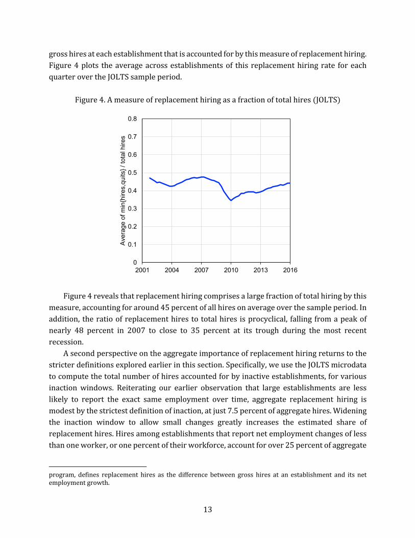
gross hires at each establishment that is accounted for by this measure of replacement hiring. Figure 4 plots the average across establishments of this replacement hiring rate for each quarter over the JOLTS sample period.

Figure 4. A measure of replacement hiring as a fraction of total hires (JOLTS)

Figure 4 reveals that replacement hiring comprises a large fraction of total hiring by this

measure, accounting for around 45 percent of all hires on average over the sample period. In addition, the ratio of replacement hires to total hires is procyclical, falling from a peak of nearly 48 percent in 2007 to close to 35 percent at its trough during the most recent recession.

A second perspective on the aggregate importance of replacement hiring returns to the stricter definitions explored earlier in this section. Specifically, we use the JOLTS microdata to compute the total number of hires accounted for by inactive establishments, for various inaction windows. Reiterating our earlier observation that large establishments are less likely to report the exact same employment over time, aggregate replacement hiring is modest by the strictest definition of inaction, at just 7.5 percent of aggregate hires. Widening the inaction window to allow small changes greatly increases the estimated share of replacement hires. Hires among establishments that report net employment changes of less than one worker, or one percent of their workforce, account for over 25 percent of aggregate

program, defines replacement hires as the difference between gross hires at an establishment and its net employment growth.

0

0.1

0.2

0.3

0.4

0.5

0.6

0.7

0.8

2001 2004 2007 2010 2013 2016

Aver

age

of m

in{h

ires,

quits

} / to

tal h

ires

14

hires. Allowing employment changes of two workers, or two percent of the workforce, raises this further to nearly 40 percent to economy-wide hiring.

3. A model of vacancy chains

The striking persistence of establishment-level employment, despite considerable gross worker turnover, suggests that employers have “reference” levels of employment to which they return routinely, often for years at a time, and do so via replacement hiring. In this section, we explore the economic implications of these stylized facts.

We argue that they call for a model with three ingredients: First, in order to map model outcomes to the preceding empirical results, it is necessary for the theory to accommodate multi-worker firms (or establishments); the one-worker-firm pair abstraction commonly invoked in canonical models, though simpler, necessarily misses this. Second, to generate endogenous quits and thereby an impetus to replacement hiring, the theory must incorporate on-the-job search, whereby employed workers contact, and sometimes transition to, alternative employers. Third, the theory must generate persistent reference levels of employment that many firms seek to return to when their workers quit. In what follows, we devise a model with these features and draw out its implications for aggregate labor market dynamics.

3.1 Matching We begin by describing the more standard aspects of the model. Consider an environment in which there is a mass of firms, normalized to one, and a mass of potential workers equal to the labor force, 𝐿𝐿. Hires in the economy are regulated by a matching technology that takes as its inputs searching workers and unfilled vacancies. Since the majority of quits transition directly from one job to another, and since our main inquiry is into the hiring behavior of firms subsequent to such quits, we allow both unemployed and, to some degree, employed workers to search for new jobs. If each of 𝑈𝑈 unemployed workers supplies one unit, and each of 𝐸𝐸 = 𝐿𝐿 − 𝑈𝑈 employed workers supplies 𝑠𝑠 units of search effort, total search effort in the economy equals 𝑈𝑈 + 𝑠𝑠(𝐿𝐿 − 𝑈𝑈). With 𝑉𝑉 unfilled vacancies, the number of new hires 𝑀𝑀 is given by the matching function, 𝑀𝑀 = 𝑀𝑀(𝑈𝑈 + 𝑠𝑠(𝐿𝐿 − 𝑈𝑈),𝑉𝑉). (1)

As is conventional, we assume that 𝑀𝑀(⋅,⋅) exhibits constant returns to scale. With random matching, it follows that a vacancy contacts a searcher with probability 𝜒𝜒(𝜃𝜃) ≡𝑀𝑀(1 𝜃𝜃⁄ , 1) , where 𝜃𝜃 ≡ 𝑉𝑉/[𝑈𝑈 + 𝑠𝑠(𝐿𝐿 − 𝑈𝑈)] represents labor market tightness. Likewise, a worker contacts a vacancy with probability 𝜙𝜙(𝜃𝜃) ≡ 𝑀𝑀(1,𝜃𝜃) per unit of search effort. As a result, an unemployed worker contacts a vacancy with probability 𝜙𝜙(𝜃𝜃), and an employed

15

worker does so with probability 𝑠𝑠𝜙𝜙(𝜃𝜃) . Note that, although the latter represent the probabilities of contact between searchers, we will see that acceptance rates will differ, as some contacts are not consummated.

3.2 The firm’s problem The problem faced by each firm in the economy mirrors in many respects that in related large-firm search and matching models that have recently been developed (Acemoglu and Hawkins 2014; Elsby and Michaels 2013). In order for the model to be able to reproduce the significant role for replacement hiring noted in the data, however, two further ingredients are added. First, we allow for on-the-job search to generate quits. Second, we incorporate a putty-clay technology with a notion of capacity that determines a reference level of employment from which it is costly for a firm to depart. We begin by describing the latter.

Capacity and the putty-clay technology. We formalize the idea of capacity by altering the production structure faced by firms. A firm employing 𝑛𝑛 workers faces a revenue function, 𝑦𝑦 = 𝑝𝑝𝑝𝑝𝑝𝑝(𝑛𝑛; 𝑘𝑘). Much of the latter is standard: 𝑝𝑝 will represent the state of aggregate labor demand (assumed constant for now); 𝑝𝑝 is an idiosyncratic shock that varies across firms and time according to the distribution function 𝐺𝐺(𝑝𝑝′|𝑝𝑝); and 𝑝𝑝(𝑛𝑛; 𝑘𝑘) is an increasing and concave function of employment 𝑛𝑛.

The key new ingredient is the presence of employment capacity, which we denote by 𝑘𝑘. This plays two roles. First, it represents a capacity constraint, such that employment at the firm cannot exceed capacity, 𝑛𝑛 ≤ 𝑘𝑘. Second, to generate incentives for replacement hiring, operating with employment below capacity induces a discrete marginal loss of output to the firm. A simple isoelastic revenue function that captures these forces is

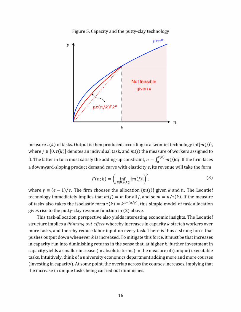
𝑝𝑝(𝑛𝑛; 𝑘𝑘) = �𝑛𝑛𝑘𝑘�𝛾𝛾𝑘𝑘𝛼𝛼 , for all 𝑛𝑛 ≤ 𝑘𝑘. (2)

Here 𝛼𝛼 ∈ (0,1) is the curvature of production when the firm operates at capacity, 𝑛𝑛 = 𝑘𝑘, and 𝛾𝛾 captures the marginal output loss from operating below capacity, 𝑛𝑛 < 𝑘𝑘. We restrict 𝛾𝛾 ∈(𝛼𝛼, 1) to capture these output losses and to preserve concavity. Figure 5 illustrates.

We refer to this production structure as “putty-clay” because it shares the notion that a firm’s technology is less flexible after it has been implemented (Fuss 1977; Malcomson and Prior 1979). Our kinked implementation of this idea resembles that in Manning (1994). We will see that this is crucial for the model’s ability to generate replacement hiring, since it implies there are costs of slack capacity.

A microfoundation. A useful interpretation of the preceding technology can be derived from a simple microeconomic model of task allocation. Suppose capacity 𝑘𝑘 is associated with

16

Figure 5. Capacity and the putty-clay technology

measure 𝜏𝜏(𝑘𝑘) of tasks. Output is then produced according to a Leontief technology inf{𝑚𝑚(𝑗𝑗)}, where 𝑗𝑗 ∈ [0, 𝜏𝜏(𝑘𝑘)] denotes an individual task, and 𝑚𝑚(𝑗𝑗) the measure of workers assigned to

it. The latter in turn must satisfy the adding-up constraint, 𝑛𝑛 = ∫ 𝑚𝑚(𝑗𝑗)d𝑗𝑗𝜏𝜏(𝑘𝑘)0 . If the firm faces

a downward-sloping product demand curve with elasticity 𝜖𝜖, its revenue will take the form

𝑝𝑝(𝑛𝑛; 𝑘𝑘) = � inf𝑗𝑗∈[0,𝜏𝜏(𝑘𝑘)]

{𝑚𝑚(𝑗𝑗)}�𝛾𝛾

, (3)

where 𝛾𝛾 ≡ (𝜖𝜖 − 1) 𝜖𝜖⁄ . The firm chooses the allocation {𝑚𝑚(𝑗𝑗)} given 𝑘𝑘 and 𝑛𝑛 . The Leontief technology immediately implies that 𝑚𝑚(𝑗𝑗) = 𝑚𝑚 for all 𝑗𝑗, and so 𝑚𝑚 = 𝑛𝑛 𝜏𝜏(𝑘𝑘)⁄ . If the measure of tasks also takes the isoelastic form 𝜏𝜏(𝑘𝑘) = 𝑘𝑘1−(𝛼𝛼 𝛾𝛾⁄ ), this simple model of task allocation gives rise to the putty-clay revenue function in (2) above.

This task-allocation perspective also yields interesting economic insights. The Leontief structure implies a thinning out effect whereby increases in capacity 𝑘𝑘 stretch workers over more tasks, and thereby reduce labor input on every task. There is thus a strong force that pushes output down whenever 𝑘𝑘 is increased. To mitigate this force, it must be that increases in capacity run into diminishing returns in the sense that, at higher 𝑘𝑘, further investment in capacity yields a smaller increase (in absolute terms) in the measure of (unique) executable tasks. Intuitively, think of a university economics department adding more and more courses (investing in capacity). At some point, the overlap across the courses increases, implying that the increase in unique tasks being carried out diminishes.

a 𝑝𝑝𝑝𝑝𝑛𝑛𝛼𝛼

a 𝑘𝑘 𝑛𝑛

given 𝑘𝑘

𝑝𝑝𝑝𝑝(𝑛𝑛/𝑘𝑘)𝛾𝛾𝑘𝑘𝛼𝛼

𝑦𝑦

17

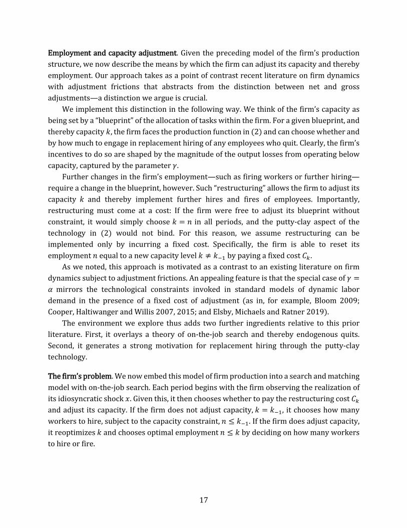
Employment and capacity adjustment. Given the preceding model of the firm’s production structure, we now describe the means by which the firm can adjust its capacity and thereby employment. Our approach takes as a point of contrast recent literature on firm dynamics with adjustment frictions that abstracts from the distinction between net and gross adjustments—a distinction we argue is crucial.

We implement this distinction in the following way. We think of the firm’s capacity as being set by a “blueprint” of the allocation of tasks within the firm. For a given blueprint, and thereby capacity 𝑘𝑘, the firm faces the production function in (2) and can choose whether and by how much to engage in replacement hiring of any employees who quit. Clearly, the firm’s incentives to do so are shaped by the magnitude of the output losses from operating below capacity, captured by the parameter 𝛾𝛾.

Further changes in the firm’s employment—such as firing workers or further hiring—require a change in the blueprint, however. Such “restructuring” allows the firm to adjust its capacity 𝑘𝑘 and thereby implement further hires and fires of employees. Importantly, restructuring must come at a cost: If the firm were free to adjust its blueprint without constraint, it would simply choose 𝑘𝑘 = 𝑛𝑛 in all periods, and the putty-clay aspect of the technology in (2) would not bind. For this reason, we assume restructuring can be implemented only by incurring a fixed cost. Specifically, the firm is able to reset its employment 𝑛𝑛 equal to a new capacity level 𝑘𝑘 ≠ 𝑘𝑘−1 by paying a fixed cost 𝐶𝐶𝑘𝑘 .

As we noted, this approach is motivated as a contrast to an existing literature on firm dynamics subject to adjustment frictions. An appealing feature is that the special case of 𝛾𝛾 =𝛼𝛼 mirrors the technological constraints invoked in standard models of dynamic labor demand in the presence of a fixed cost of adjustment (as in, for example, Bloom 2009; Cooper, Haltiwanger and Willis 2007, 2015; and Elsby, Michaels and Ratner 2019).

The environment we explore thus adds two further ingredients relative to this prior literature. First, it overlays a theory of on-the-job search and thereby endogenous quits. Second, it generates a strong motivation for replacement hiring through the putty-clay technology.

The firm’s problem. We now embed this model of firm production into a search and matching model with on-the-job search. Each period begins with the firm observing the realization of its idiosyncratic shock 𝑝𝑝. Given this, it then chooses whether to pay the restructuring cost 𝐶𝐶𝑘𝑘 and adjust its capacity. If the firm does not adjust capacity, 𝑘𝑘 = 𝑘𝑘−1, it chooses how many workers to hire, subject to the capacity constraint, 𝑛𝑛 ≤ 𝑘𝑘−1. If the firm does adjust capacity, it reoptimizes 𝑘𝑘 and chooses optimal employment 𝑛𝑛 ≤ 𝑘𝑘 by deciding on how many workers to hire or fire.

18

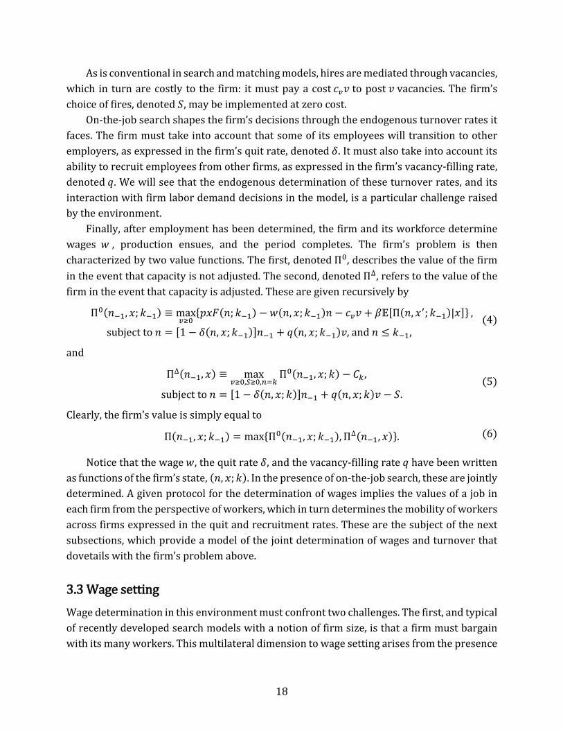
As is conventional in search and matching models, hires are mediated through vacancies, which in turn are costly to the firm: it must pay a cost 𝑐𝑐𝑣𝑣𝑣𝑣 to post 𝑣𝑣 vacancies. The firm’s choice of fires, denoted 𝑆𝑆, may be implemented at zero cost.

On-the-job search shapes the firm’s decisions through the endogenous turnover rates it faces. The firm must take into account that some of its employees will transition to other employers, as expressed in the firm’s quit rate, denoted 𝛿𝛿. It must also take into account its ability to recruit employees from other firms, as expressed in the firm’s vacancy-filling rate, denoted 𝑞𝑞. We will see that the endogenous determination of these turnover rates, and its interaction with firm labor demand decisions in the model, is a particular challenge raised by the environment.

Finally, after employment has been determined, the firm and its workforce determine wages 𝑤𝑤 , production ensues, and the period completes. The firm’s problem is then characterized by two value functions. The first, denoted Π0, describes the value of the firm in the event that capacity is not adjusted. The second, denoted Π∆, refers to the value of the firm in the event that capacity is adjusted. These are given recursively by

Π0(𝑛𝑛−1, 𝑝𝑝; 𝑘𝑘−1) ≡ max𝑣𝑣≥0

{𝑝𝑝𝑝𝑝𝑝𝑝(𝑛𝑛; 𝑘𝑘−1) − 𝑤𝑤(𝑛𝑛, 𝑝𝑝; 𝑘𝑘−1)𝑛𝑛 − 𝑐𝑐𝑣𝑣𝑣𝑣 + 𝛽𝛽𝛽𝛽[Π(𝑛𝑛, 𝑝𝑝′; 𝑘𝑘−1)|𝑝𝑝]} ,

subject to 𝑛𝑛 = [1 − 𝛿𝛿(𝑛𝑛, 𝑝𝑝; 𝑘𝑘−1)]𝑛𝑛−1 + 𝑞𝑞(𝑛𝑛, 𝑝𝑝; 𝑘𝑘−1)𝑣𝑣, and 𝑛𝑛 ≤ 𝑘𝑘−1, (4)

and

Π∆(𝑛𝑛−1, 𝑝𝑝) ≡ max𝑣𝑣≥0,𝑆𝑆≥0,𝑛𝑛=𝑘𝑘

Π0(𝑛𝑛−1, 𝑝𝑝; 𝑘𝑘) − 𝐶𝐶𝑘𝑘,

subject to 𝑛𝑛 = [1 − 𝛿𝛿(𝑛𝑛, 𝑝𝑝; 𝑘𝑘)]𝑛𝑛−1 + 𝑞𝑞(𝑛𝑛, 𝑝𝑝; 𝑘𝑘)𝑣𝑣 − 𝑆𝑆. (5)

Clearly, the firm’s value is simply equal to

Π(𝑛𝑛−1, 𝑝𝑝; 𝑘𝑘−1) = max{Π0(𝑛𝑛−1, 𝑝𝑝; 𝑘𝑘−1),Π∆(𝑛𝑛−1, 𝑝𝑝)}. (6)

Notice that the wage 𝑤𝑤, the quit rate 𝛿𝛿, and the vacancy-filling rate 𝑞𝑞 have been written as functions of the firm’s state, (𝑛𝑛, 𝑝𝑝; 𝑘𝑘). In the presence of on-the-job search, these are jointly determined. A given protocol for the determination of wages implies the values of a job in each firm from the perspective of workers, which in turn determines the mobility of workers across firms expressed in the quit and recruitment rates. These are the subject of the next subsections, which provide a model of the joint determination of wages and turnover that dovetails with the firm’s problem above.

3.3 Wage setting Wage determination in this environment must confront two challenges. The first, and typical of recently developed search models with a notion of firm size, is that a firm must bargain with its many workers. This multilateral dimension to wage setting arises from the presence

19

of decreasing returns in production, which implies that the surpluses generated by each of the workers in the firm are not independent of one another. The second challenge relates to how wages are determined when an employed worker meets another firm, which emerges from the presence of on-the-job search.

Given our focus on capturing the replacement hiring motive, and the requisite complexity of the production structure that accompanies it, our goal is to implement a wage setting protocol that is as simple as possible, subject to the requirements of internal coherence and broad consistency with known empirical properties of wages. In this spirit, our strategy is to implement the approach to wage determination set out in Elsby and Gottfries (2019). This combines the insights of credible bargaining (Binmore et al. 1986), multilateral bargaining (Bruegemann et al. 2018), and ex post bargaining in the presence of on-the-job search (Gottfries 2019).12F

13 Each period, after idiosyncratic productivity has been realized and employment

determined, the firm and its workers bargain over the flow wage for that period. Following Bruegemann, Gautier, and Menzio (2018), the firm engages in a sequence of bilateral bargaining sessions with each of its workers in an extensive form that mirrors a Rolodex. This sequence of play is devised in such a way that the workers’ strategic positions are symmetric. As a result, Bruegemann et al. show that this “Rolodex” game gives rise to an equilibrium in which all workers within the firm are paid a common wage that corresponds to a simple marginal surplus sharing rule proposed by Stole and Zwiebel (1996).

The relevant marginal surplus is determined in turn by the threats that the firm and its workers can credibly issue in the course of the bargain. Following Binmore, Rubinstein, and Wolinsky (1986), we assume that threats of permanent severance are not credible: following any breakdown of negotiations between the firm and a given worker, it will be optimal for both parties to reenter negotiations next period. Instead, the firm and worker can credibly threaten only a temporary disruption of production in the current period. Hall and Milgrom (2008) apply similar ideas in the context of the canonical Diamond-Mortensen-Pissarides search and matching model. A useful implication for our purposes is that, in combination with renegotiation each period, it follows that the firm and its workers effectively bargain over the marginal flow surplus.

This approach to wage determination satisfies all of our stated goals. Chief among these is its relative simplicity. In particular, following Hall and Milgrom, if in the event of breakdown the firm faces a flow cost of 𝑏𝑏𝑓𝑓, and the worker a flow payoff of 𝑏𝑏𝑤𝑤, then marginal flow surplus sharing implies

13 An alternative to this approach to wage setting proposes instead that, in the event a worker is contacted by an outside employer, the rival firms engage in Bertrand competition over that worker (Postel-Vinay and Robin 2002). As discussed in Elsby and Gottfries (2019), possible motivations for the absence of offer matching include lack of verifiability of outside offers and equal treatment constraints within the firm.

20

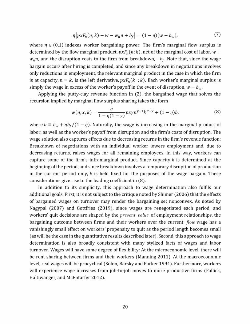
𝜂𝜂�𝑝𝑝𝑝𝑝𝑝𝑝𝑛𝑛(𝑛𝑛; 𝑘𝑘) − 𝑤𝑤 − 𝑤𝑤𝑛𝑛𝑛𝑛 + 𝑏𝑏𝑓𝑓� = (1 − 𝜂𝜂)(𝑤𝑤 − 𝑏𝑏𝑤𝑤), (7)

where 𝜂𝜂 ∈ (0,1) indexes worker bargaining power. The firm’s marginal flow surplus is determined by the flow marginal product, 𝑝𝑝𝑝𝑝𝑝𝑝𝑛𝑛(𝑛𝑛; 𝑘𝑘), net of the marginal cost of labor, 𝑤𝑤 +𝑤𝑤𝑛𝑛𝑛𝑛, and the disruption costs to the firm from breakdown, −𝑏𝑏𝑓𝑓. Note that, since the wage bargain occurs after hiring is completed, and since any breakdown in negotiations involves only reductions in employment, the relevant marginal product in the case in which the firm is at capacity, 𝑛𝑛 = 𝑘𝑘, is the left derivative, 𝑝𝑝𝑝𝑝𝑝𝑝𝑛𝑛(𝑘𝑘−; 𝑘𝑘). Each worker’s marginal surplus is simply the wage in excess of the worker’s payoff in the event of disruption, 𝑤𝑤 − 𝑏𝑏𝑤𝑤.

Applying the putty-clay revenue function in (2), the bargained wage that solves the recursion implied by marginal flow surplus sharing takes the form

𝑤𝑤(𝑛𝑛, 𝑝𝑝; 𝑘𝑘) =𝜂𝜂

1 − 𝜂𝜂(1 − 𝛾𝛾) 𝑝𝑝𝑝𝑝𝛾𝛾𝑛𝑛𝛾𝛾−1𝑘𝑘𝛼𝛼−𝛾𝛾 + (1 − 𝜂𝜂)𝑏𝑏, (8)

where 𝑏𝑏 ≡ 𝑏𝑏𝑤𝑤 + 𝜂𝜂𝑏𝑏𝑓𝑓 (1 − 𝜂𝜂)⁄ . Naturally, the wage is increasing in the marginal product of labor, as well as the worker’s payoff from disruption and the firm’s costs of disruption. The wage solution also captures effects due to decreasing returns in the firm’s revenue function: Breakdown of negotiations with an individual worker lowers employment and, due to decreasing returns, raises wages for all remaining employees. In this way, workers can capture some of the firm’s inframarginal product. Since capacity 𝑘𝑘 is determined at the beginning of the period, and since breakdown involves a temporary disruption of production in the current period only, 𝑘𝑘 is held fixed for the purposes of the wage bargain. These considerations give rise to the leading coefficient in (8).

In addition to its simplicity, this approach to wage determination also fulfils our additional goals. First, it is not subject to the critique noted by Shimer (2006) that the effects of bargained wages on turnover may render the bargaining set nonconvex. As noted by Nagypal (2007) and Gottfries (2019), since wages are renegotiated each period, and workers’ quit decisions are shaped by the present value of employment relationships, the bargaining outcome between firms and their workers over the current flow wage has a vanishingly small effect on workers’ propensity to quit as the period length becomes small (as will be the case in the quantitative results described later). Second, this approach to wage determination is also broadly consistent with many stylized facts of wages and labor turnover. Wages will have some degree of flexibility: At the microeconomic level, there will be rent sharing between firms and their workers (Manning 2011). At the macroeconomic level, real wages will be procyclical (Solon, Barsky and Parker 1994). Furthermore, workers will experience wage increases from job-to-job moves to more productive firms (Fallick, Haltiwanger, and McEntarfer 2012).

21

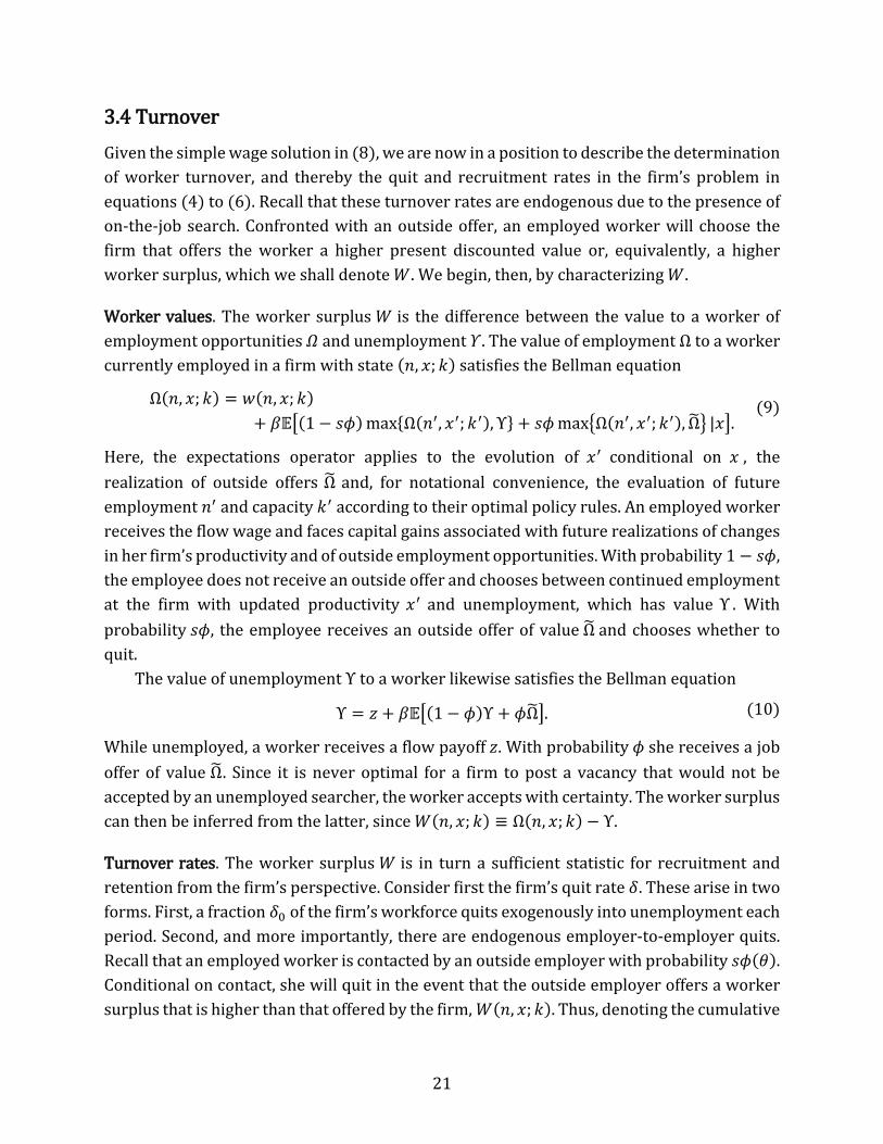
3.4 Turnover Given the simple wage solution in (8), we are now in a position to describe the determination of worker turnover, and thereby the quit and recruitment rates in the firm’s problem in equations (4) to (6). Recall that these turnover rates are endogenous due to the presence of on-the-job search. Confronted with an outside offer, an employed worker will choose the firm that offers the worker a higher present discounted value or, equivalently, a higher worker surplus, which we shall denote 𝑊𝑊. We begin, then, by characterizing 𝑊𝑊.

Worker values. The worker surplus 𝑊𝑊 is the difference between the value to a worker of employment opportunities 𝛺𝛺 and unemployment 𝛶𝛶. The value of employment Ω to a worker currently employed in a firm with state (𝑛𝑛, 𝑝𝑝; 𝑘𝑘) satisfies the Bellman equation

Ω(𝑛𝑛, 𝑝𝑝; 𝑘𝑘) = 𝑤𝑤(𝑛𝑛, 𝑝𝑝; 𝑘𝑘)+ 𝛽𝛽𝛽𝛽�(1 − 𝑠𝑠𝜙𝜙) max{Ω(𝑛𝑛′, 𝑝𝑝′; 𝑘𝑘′),Υ} + 𝑠𝑠𝜙𝜙max�Ω(𝑛𝑛′, 𝑝𝑝′; 𝑘𝑘′),Ω�� |𝑝𝑝�.

(9)

Here, the expectations operator applies to the evolution of 𝑝𝑝′ conditional on 𝑝𝑝 , the realization of outside offers Ω� and, for notational convenience, the evaluation of future employment 𝑛𝑛′ and capacity 𝑘𝑘′ according to their optimal policy rules. An employed worker receives the flow wage and faces capital gains associated with future realizations of changes in her firm’s productivity and of outside employment opportunities. With probability 1 − 𝑠𝑠𝜙𝜙, the employee does not receive an outside offer and chooses between continued employment at the firm with updated productivity 𝑝𝑝′ and unemployment, which has value Υ . With probability 𝑠𝑠𝜙𝜙, the employee receives an outside offer of value Ω� and chooses whether to quit.

The value of unemployment Υ to a worker likewise satisfies the Bellman equation

Υ = 𝑧𝑧 + 𝛽𝛽𝛽𝛽�(1 − 𝜙𝜙)Υ + 𝜙𝜙Ω��. (10)

While unemployed, a worker receives a flow payoff 𝑧𝑧. With probability 𝜙𝜙 she receives a job offer of value Ω� . Since it is never optimal for a firm to post a vacancy that would not be accepted by an unemployed searcher, the worker accepts with certainty. The worker surplus can then be inferred from the latter, since 𝑊𝑊(𝑛𝑛, 𝑝𝑝; 𝑘𝑘) ≡ Ω(𝑛𝑛, 𝑝𝑝; 𝑘𝑘) − Υ.

Turnover rates. The worker surplus 𝑊𝑊 is in turn a sufficient statistic for recruitment and retention from the firm’s perspective. Consider first the firm’s quit rate 𝛿𝛿. These arise in two forms. First, a fraction 𝛿𝛿0 of the firm’s workforce quits exogenously into unemployment each period. Second, and more importantly, there are endogenous employer-to-employer quits. Recall that an employed worker is contacted by an outside employer with probability 𝑠𝑠𝜙𝜙(𝜃𝜃). Conditional on contact, she will quit in the event that the outside employer offers a worker surplus that is higher than that offered by the firm, 𝑊𝑊(𝑛𝑛, 𝑝𝑝; 𝑘𝑘). Thus, denoting the cumulative

22

distribution function of worker surpluses among vacancy-posting firms by Φ(⋅), the quit rate is therefore given by

𝛿𝛿(𝑛𝑛, 𝑝𝑝; 𝑘𝑘) = 𝛿𝛿0 + 𝑠𝑠𝜙𝜙(𝜃𝜃)�1 −Φ�𝑊𝑊(𝑛𝑛, 𝑝𝑝; 𝑘𝑘)��. (11)

Now consider the vacancy-filling rate faced by the firm 𝑞𝑞. Recall that, with probability 𝜒𝜒(𝜃𝜃), a vacancy-posting firm meets a searching worker. The firm will contact an unemployed worker with probability 𝜓𝜓 ≡ 𝑈𝑈/[𝑈𝑈 + 𝑠𝑠(𝐿𝐿 − 𝑈𝑈)]. Since hiring firms face a positive marginal cost to posting vacancies, they would never post a vacancy that is not accepted by an unemployed searcher. Consequently, they will hire unemployed job seekers with certainty. With complementary probability, 1 − 𝜓𝜓, the firm will contact an employed searcher. The firm will hire the searcher in the event that the searcher currently receives a worker surplus that is lower than that offered by the firm, 𝑊𝑊(𝑛𝑛, 𝑝𝑝; 𝑘𝑘). Denoting the cumulative distribution function of worker surpluses among employed workers by Γ(⋅), the vacancy-filling rate is therefore given by

𝑞𝑞(𝑛𝑛, 𝑝𝑝; 𝑘𝑘) = 𝜒𝜒(𝜃𝜃)�𝜓𝜓 + (1 − 𝜓𝜓)Γ�𝑊𝑊(𝑛𝑛, 𝑝𝑝; 𝑘𝑘)��. (12)

In combination with the firm’s problem in equations (4) to (6), the wage solution in (8) and the quit and recruitment rates in (11) and (12) complete the description of the environment.

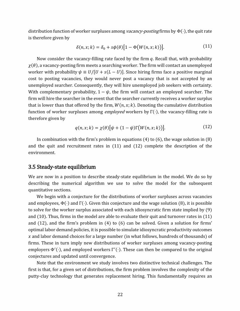
3.5 Steady-state equilibrium We are now in a position to describe steady-state equilibrium in the model. We do so by describing the numerical algorithm we use to solve the model for the subsequent quantitative sections.

We begin with a conjecture for the distributions of worker surpluses across vacancies and employees, Φ(⋅) and Γ(⋅). Given this conjecture and the wage solution (8), it is possible to solve for the worker surplus associated with each idiosyncratic firm state implied by (9) and (10). Thus, firms in the model are able to evaluate their quit and turnover rates in (11) and (12), and the firm’s problem in (4) to (6) can be solved. Given a solution for firms’ optimal labor demand policies, it is possible to simulate idiosyncratic productivity outcomes 𝑝𝑝 and labor demand choices for a large number (in what follows, hundreds of thousands) of firms. These in turn imply new distributions of worker surpluses among vacancy-posting employers Φ′(⋅), and employed workers Γ′(⋅). These can then be compared to the original conjectures and updated until convergence.

Note that the environment we study involves two distinctive technical challenges. The first is that, for a given set of distributions, the firm problem involves the complexity of the putty-clay technology that generates replacement hiring. This fundamentally requires an

23

additional state variable, capacity 𝑘𝑘 , that carries information on replacement incentives. Second, and more daunting, the aggregate state includes the distributions of workers surpluses Φ(⋅) and Γ(⋅) that both inform firms’ labor demand decisions and are implied by the aggregate outcomes of those same decisions. Thus, steady-state equilibrium involves a fixed point in these distributions. This is much more technically challenging than related heterogenous agent economies in which agents must forecast an equilibrium price (as in Krusell and Smith 1998, and the large literature it has inspired). The analogue in the present environment is that agents have to forecast entire equilibrium functions—the distributions Φ(⋅) and Γ(⋅) or, equivalently, the quit and recruitment rates 𝛿𝛿(⋅) and 𝑞𝑞(⋅). Out of steady state, dynamic equilibrium further requires solution of a fixed point in the dynamic path of these functions. While some progress has been made on this problem for simpler economies with on-the-job search (see Elsby and Gottfries 2019), the present environment involves the further complexity of accommodating a replacement hiring motive. For this reason, in what follows we focus on steady-state responses.

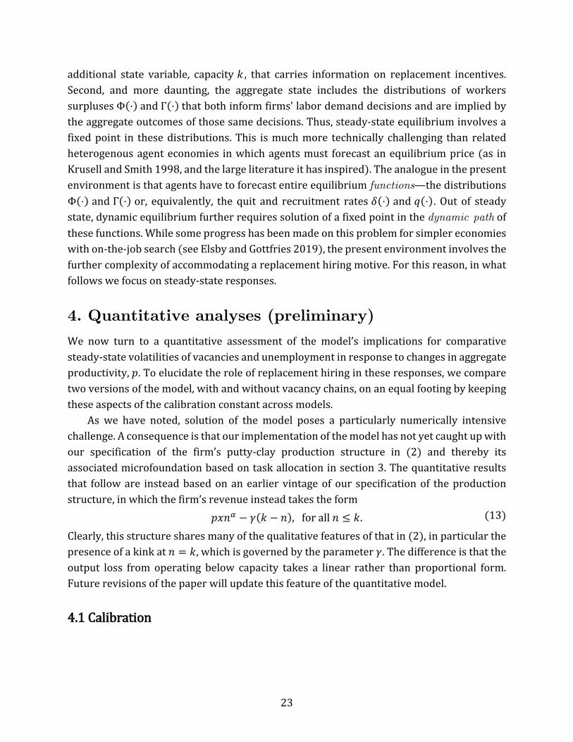
4. Quantitative analyses (preliminary)

We now turn to a quantitative assessment of the model’s implications for comparative steady-state volatilities of vacancies and unemployment in response to changes in aggregate productivity, 𝑝𝑝. To elucidate the role of replacement hiring in these responses, we compare two versions of the model, with and without vacancy chains, on an equal footing by keeping these aspects of the calibration constant across models.

As we have noted, solution of the model poses a particularly numerically intensive challenge. A consequence is that our implementation of the model has not yet caught up with our specification of the firm’s putty-clay production structure in (2) and thereby its associated microfoundation based on task allocation in section 3. The quantitative results that follow are instead based on an earlier vintage of our specification of the production structure, in which the firm’s revenue instead takes the form 𝑝𝑝𝑝𝑝𝑛𝑛𝛼𝛼 − 𝛾𝛾(𝑘𝑘 − 𝑛𝑛), for all 𝑛𝑛 ≤ 𝑘𝑘. (13)

Clearly, this structure shares many of the qualitative features of that in (2), in particular the presence of a kink at 𝑛𝑛 = 𝑘𝑘, which is governed by the parameter 𝛾𝛾. The difference is that the output loss from operating below capacity takes a linear rather than proportional form. Future revisions of the paper will update this feature of the quantitative model.

4.1 Calibration

24

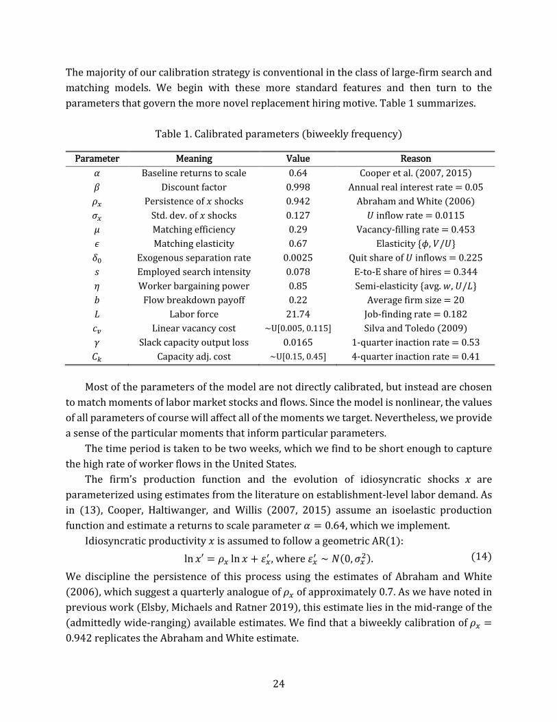
The majority of our calibration strategy is conventional in the class of large-firm search and matching models. We begin with these more standard features and then turn to the parameters that govern the more novel replacement hiring motive. Table 1 summarizes.

Table 1. Calibrated parameters (biweekly frequency)

Parameter Meaning Value Reason 𝛼𝛼 Baseline returns to scale 0.64 Cooper et al. (2007, 2015) 𝛽𝛽 Discount factor 0.998 Annual real interest rate = 0.05 𝜌𝜌𝑥𝑥 Persistence of 𝑝𝑝 shocks 0.942 Abraham and White (2006) 𝜎𝜎𝑥𝑥 Std. dev. of 𝑝𝑝 shocks 0.127 𝑈𝑈 inflow rate = 0.0115 𝜇𝜇 Matching efficiency 0.29 Vacancy-filling rate = 0.453 𝜖𝜖 Matching elasticity 0.67 Elasticity {𝜙𝜙, 𝑉𝑉/𝑈𝑈} 𝛿𝛿0 Exogenous separation rate 0.0025 Quit share of 𝑈𝑈 inflows = 0.225 𝑠𝑠 Employed search intensity 0.078 E-to-E share of hires = 0.344 𝜂𝜂 Worker bargaining power 0.85 Semi-elasticity {avg. 𝑤𝑤, 𝑈𝑈/𝐿𝐿} 𝑏𝑏 Flow breakdown payoff 0.22 Average firm size = 20 𝐿𝐿 Labor force 21.74 Job-finding rate = 0.182 𝑐𝑐𝑣𝑣 Linear vacancy cost ∼U[0.005, 0.115] Silva and Toledo (2009) 𝛾𝛾 Slack capacity output loss 0.0165 1-quarter inaction rate = 0.53 𝐶𝐶𝑘𝑘 Capacity adj. cost ∼U[0.15, 0.45] 4-quarter inaction rate = 0.41

Most of the parameters of the model are not directly calibrated, but instead are chosen to match moments of labor market stocks and flows. Since the model is nonlinear, the values of all parameters of course will affect all of the moments we target. Nevertheless, we provide a sense of the particular moments that inform particular parameters.

The time period is taken to be two weeks, which we find to be short enough to capture the high rate of worker flows in the United States.

The firm’s production function and the evolution of idiosyncratic shocks 𝑝𝑝 are parameterized using estimates from the literature on establishment-level labor demand. As in (13), Cooper, Haltiwanger, and Willis (2007, 2015) assume an isoelastic production function and estimate a returns to scale parameter 𝛼𝛼 = 0.64, which we implement.

Idiosyncratic productivity 𝑝𝑝 is assumed to follow a geometric AR(1): ln 𝑝𝑝′ = 𝜌𝜌𝑥𝑥 ln 𝑝𝑝 + 𝜀𝜀𝑥𝑥′ , where 𝜀𝜀𝑥𝑥′ ∼ 𝑁𝑁(0,𝜎𝜎𝑥𝑥2). (14)

We discipline the persistence of this process using the estimates of Abraham and White (2006), which suggest a quarterly analogue of 𝜌𝜌𝑥𝑥 of approximately 0.7. As we have noted in previous work (Elsby, Michaels and Ratner 2019), this estimate lies in the mid-range of the (admittedly wide-ranging) available estimates. We find that a biweekly calibration of 𝜌𝜌𝑥𝑥 = 0.942 replicates the Abraham and White estimate.

25

The standard deviation of the innovations to idiosyncratic productivity 𝜎𝜎𝑥𝑥 is chosen to replicate the empirical biweekly unemployment inflow rate of 0.0115. Intuitively, fixing all other parameter values, greater idiosyncratic variance will increase the likelihood that firms realize large adverse shocks that induce them to fire workers. We find that a biweekly calibration of 𝜎𝜎𝑥𝑥 = 0.127 replicates the unemployment inflow rate.

We assume that the matching function is of the conventional constant-returns Cobb-Douglas form, 𝑀𝑀 = 𝜇𝜇[𝑈𝑈 + 𝑠𝑠(𝐿𝐿 − 𝑈𝑈)]𝜖𝜖𝑉𝑉1−𝜖𝜖 . We set the matching elasticity to 𝜖𝜖 = 0.67 to replicate the empirical elasticity of the job-finding rate with respect to the vacancy-unemployment ratio. Matching efficiency 𝜇𝜇 is chosen such that, given all other parameters, the average biweekly vacancy-filling rate is equal to 0.453, as implied by the monthly estimates of Davis, Faberman and Haltiwanger (2006, 2013) using JOLTS data.

The rate of exogenous separations into unemployment 𝛿𝛿0 is chosen to replicate the share of workers who flow into unemployment and report having quit their job. Publicly available BLS data suggest that 22.5 percent of unemployment inflows are coded as “job leavers” in the Current Population Survey. Thus, we set 𝛿𝛿0 = 0.225 × 0.0115 = 0.0025 to match this moment.

To calibrate the search intensity of the employed 𝑠𝑠 we target the fraction of total hires accounted for by job-to-job flows. Fallick and Fleischman (2004) estimate the latter to be close to 35 percent. Together with the rest of our calibration, we find that 𝑠𝑠 = 0.078 matches this moment.

Worker bargaining power 𝜂𝜂 shapes the response of real wages to changes in labor productivity. Motivated by this, and since we are interested in labor market responses to aggregate shocks, we choose 𝜂𝜂 to accommodate empirical estimates that suggest that, once adjustments are made for cyclical shifts in worker composition, real wages are procyclical (Solon, Barsky and Parker 1994). We find that setting 𝜂𝜂 = 0.85 gives rise to a steady-state semi-elasticity of average real wages with respect to the unemployment rate of -0.77. This lies in the neighborhood of the estimates of Elsby, Shin and Solon (2016) (for men; estimates for women are more sensitive to estimated trends in female wages).

The flow payoff from breakdown in wage negotiations 𝑏𝑏 has a direct influence on the level of wages relative to the marginal product in the wage equation (8). Consequently, we use 𝑏𝑏 to replicate average firm size. Data from the Small Business Administration suggest the latter is around 20, and we find that a biweekly value of 𝑏𝑏 = 0.22 hits that moment. Since Hagedorn and Manovskii (2008), the magnitude of (analogues of) 𝑏𝑏 in relation to labor productivity has been recognized as a key determinant of the amplification of unemployment and vacancy responses to changes in aggregate productivity. For this reason, we also report the value of 𝑏𝑏 relative to the average product of labor in the model economy, which is 61 percent. This value lies toward the lower range of values in the literature.

26

Given labor productivity, a larger labor force 𝐿𝐿 will clearly be associated with greater unemployment all else equal. Thus, we set 𝐿𝐿 = 21.74 to replicate a biweekly job-finding rate among the unemployed of 0.182. Equivalently, given that we have already targeted a biweekly unemployment inflow rate of 0.0115, our strategy also matches a steady-state unemployment rate of a little under 6 percent.

Our final standard parameter is the linear vacancy-posting cost, 𝑐𝑐𝑣𝑣 . We use these to capture two forces. First, we allow firms to face permanent heterogeneity in their vacancy costs. This contributes to heterogeneity in marginal job values in hiring firms, and thereby to heterogeneity in worker surpluses across vacancies and employees captured in the distributions Φ(⋅) and Γ(⋅) . We implement this as simply as possible by allowing for a uniform distribution of vacancy costs across firms, 𝑐𝑐𝑣𝑣 ∼ 𝑈𝑈�𝑐𝑐𝑣𝑣� , 𝑐𝑐𝑣𝑣� �. Second, we then calibrate the mean of the distribution of vacancy costs, �𝑐𝑐𝑣𝑣� + 𝑐𝑐𝑣𝑣� � 2⁄ . Definitive empirical evidence on the average magnitude of vacancy costs is limited, however. Consequently, we broadly target the evidence from Silva and Toledo (2009) suggesting that per-worker hiring costs correspond to around 2 days of earnings, but allow the model to deviate more on this moment relative to the others.13F

14

Replacement hiring parameters. We now turn to the calibration of the more distinctive elements of the model, those that govern employment inaction and capacity adjustment and thereby replacement hiring.

In the model, inaction in net establishment employment growth is determined by the marginal output losses from operating below capacity, captured by the parameter 𝛾𝛾 and the fixed costs of changing capacity, 𝐶𝐶𝑘𝑘 . Absent these elements, the presence of job-to-job quits in the model and vacancy-posting costs would generate inaction at zero gross employment change—that is, a discrete fraction of firms would engage in neither gross hiring nor gross firing and would retain a reduced stock of workers who have not quit. There would be no net inaction. Thus, the impetus for a firm to return to its prior employment level arises if the loss of output due to slack capacity 𝛾𝛾 and the costs of adjusting capacity 𝐶𝐶𝑘𝑘 are sufficiently high relative to vacancy-posting costs 𝑐𝑐𝑣𝑣.

With this in mind, we calibrate the slack cost 𝛾𝛾 to target the observed net inaction rate of roughly 55 percent seen in the QCEW microdata documented in section 1. We find that this implies a slack cost of 𝛾𝛾 = 0.0165.

We allow the fixed cost of adjusting capacity 𝐶𝐶𝑘𝑘 to vary within a firm over time. Specifically, each period a firm draws a fixed cost from a simple uniform distribution, 𝐶𝐶𝑘𝑘 ∼

14 Manning (2011) reports a range of estimates from much less than one week of wages to about six weeks. Note, however, that our calculation omits any costs of hiring associated with expanding capacity, which we will see is subject to large costs.

27

𝑈𝑈�𝐶𝐶𝑘𝑘���,𝐶𝐶𝑘𝑘����. We do this because the data demand large capacity adjustment costs to replicate the degree of replacement hiring. Such large fixed costs of adjustment induce strong nonlinearities in the model. The presence of time-varying capacity adjustment costs helps to smooth out the firm’s problem and induce stable numerical solutions for firm labor demand. We then calibrate the average cost of capacity adjustment �𝐶𝐶𝑘𝑘��� + 𝐶𝐶𝑘𝑘���� 2⁄ to target the slow decay of net inaction by frequency of adjustment noted in section 1. Intuitively, for as long as a particular level of capacity remains, it will serve as an anchor for the desired level of employment, and the firm will have an incentive to return to that level routinely. In this way, the rate of capacity adjustment informs the likelihood that a firm returns to a reference employment level after several periods and thereby the endogenous decay of employment inaction in equilibrium. We target the four-quarter employment inaction rate of 41 percent from the QCEW microdata underlying Figure 2A. This approach gives rise to an average cost of capacity adjustment �𝐶𝐶𝑘𝑘��� + 𝐶𝐶𝑘𝑘���� 2⁄ that corresponds to 30 percent of average frictionless biweekly revenue.

4.2 Replacement hiring in the model We now return to the facts on replacement hiring documented in section 2 and assess the ability of the model to replicate them. The first panel of Table 2 takes each of the facts in turn and compares their empirical values with the outcomes in two versions of the model. The first is calibrated as above. The second suspends the costs of adjusting capacity, 𝛾𝛾 = 𝐶𝐶𝑘𝑘 ≡ 0, and recalibrates to match all the targets in Table 1, except the one- and four-quarter net inaction rates (which, as we have discussed, this model is intrinsically unable to generate).

The ability of the model with capacity frictions to match the facts on replacement hiring is encouraging. It is able to match closely the first fact: that there is significant inaction over net employment changes. The model implies a one-quarter net inaction rate of 54 percent, very close to its empirical analogue. It is also able to generate considerable persistence in net inaction, mirroring the slow decay of inaction in Figure 2. The four-quarter net inaction rate implied by the model is 37 percent, just a little below its empirical counterpart of 41 percent. Of course, as anticipated, the model without capacity is unable to generate net inaction at any frequency. The fact that the model with capacity can engage with these stylized facts is thus an important success.

The next row of Table 2 makes clear how the model with capacity frictions achieves these results. The quarterly capacity adjustment rate in the model is just 9 percent. Thus 𝑘𝑘 in the model is very persistent at the firm level and acts as an anchor for employment that firms return to in the future.

28

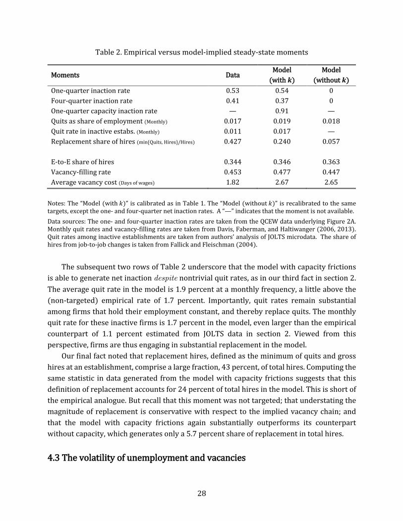
Table 2. Empirical versus model-implied steady-state moments

Moments Data Model

(with 𝒌𝒌) Model

(without 𝒌𝒌) One-quarter inaction rate 0.53 0.54 0 Four-quarter inaction rate 0.41 0.37 0 One-quarter capacity inaction rate — 0.91 — Quits as share of employment (Monthly) 0.017 0.019 0.018 Quit rate in inactive estabs. (Monthly) 0.011 0.017 — Replacement share of hires (min{Quits, Hires}/Hires) 0.427 0.240 0.057 E-to-E share of hires 0.344 0.346 0.363 Vacancy-filling rate 0.453 0.477 0.447 Average vacancy cost (Days of wages) 1.82 2.67 2.65

Notes: The “Model (with 𝑘𝑘)” is calibrated as in Table 1. The “Model (without 𝑘𝑘)” is recalibrated to the same targets, except the one- and four-quarter net inaction rates. A “—” indicates that the moment is not available. Data sources: The one- and four-quarter inaction rates are taken from the QCEW data underlying Figure 2A. Monthly quit rates and vacancy-filling rates are taken from Davis, Faberman, and Haltiwanger (2006, 2013). Quit rates among inactive establishments are taken from authors’ analysis of JOLTS microdata. The share of hires from job-to-job changes is taken from Fallick and Fleischman (2004).

The subsequent two rows of Table 2 underscore that the model with capacity frictions

is able to generate net inaction despite nontrivial quit rates, as in our third fact in section 2. The average quit rate in the model is 1.9 percent at a monthly frequency, a little above the (non-targeted) empirical rate of 1.7 percent. Importantly, quit rates remain substantial among firms that hold their employment constant, and thereby replace quits. The monthly quit rate for these inactive firms is 1.7 percent in the model, even larger than the empirical counterpart of 1.1 percent estimated from JOLTS data in section 2. Viewed from this perspective, firms are thus engaging in substantial replacement in the model.

Our final fact noted that replacement hires, defined as the minimum of quits and gross hires at an establishment, comprise a large fraction, 43 percent, of total hires. Computing the same statistic in data generated from the model with capacity frictions suggests that this definition of replacement accounts for 24 percent of total hires in the model. This is short of the empirical analogue. But recall that this moment was not targeted; that understating the magnitude of replacement is conservative with respect to the implied vacancy chain; and that the model with capacity frictions again substantially outperforms its counterpart without capacity, which generates only a 5.7 percent share of replacement in total hires.

4.3 The volatility of unemployment and vacancies

29

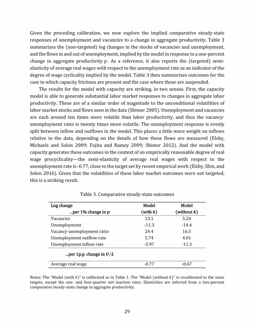
Given the preceding calibration, we now explore the implied comparative steady-state responses of unemployment and vacancies to a change in aggregate productivity. Table 3 summarizes the (non-targeted) log changes in the stocks of vacancies and unemployment, and the flows in and out of unemployment, implied by the model in response to a one-percent change in aggregate productivity 𝑝𝑝 . As a reference, it also reports the (targeted) semi-elasticity of average real wages with respect to the unemployment rate as an indicator of the degree of wage cyclicality implied by the model. Table 3 then summarizes outcomes for the case in which capacity frictions are present and the case where these are suspended.

The results for the model with capacity are striking, in two senses. First, the capacity model is able to generate substantial labor market responses to changes in aggregate labor productivity. These are of a similar order of magnitude to the unconditional volatilities of labor market stocks and flows seen in the data (Shimer 2005). Unemployment and vacancies are each around ten times more volatile than labor productivity, and thus the vacancy-unemployment ratio is twenty times more volatile. The unemployment response is evenly split between inflow and outflows in the model. This places a little more weight on inflows relative to the data, depending on the details of how these flows are measured (Elsby, Michaels and Solon 2009; Fujita and Ramey 2009; Shimer 2012). And the model with capacity generates these outcomes in the context of an empirically reasonable degree of real wage procyclicality—the semi-elasticity of average real wages with respect to the unemployment rate is -0.77, close to the target set by recent empirical work (Elsby, Shin, and Solon 2016). Given that the volatilities of these labor market outcomes were not targeted, this is a striking result.

Table 3. Comparative steady-state outcomes

Log change …per 1% change in 𝒑𝒑

Model (with 𝒌𝒌)

Model (without 𝒌𝒌)

Vacancies 13.1 5.24 Unemployment -11.3 -14.4 Vacancy-unemployment ratio 24.4 16.5 Unemployment outflow rate 5.74 4.01 Unemployment inflow rate -5.97 -11.3

…per 1p.p. change in 𝑼𝑼/𝑳𝑳

Average real wage -0.77 -0.67 Notes: The “Model (with 𝑘𝑘)” is calibrated as in Table 1. The “Model (without 𝑘𝑘)” is recalibrated to the same targets, except the one- and four-quarter net inaction rates. Elasticities are inferred from a two-percent comparative steady-state change in aggregate productivity.

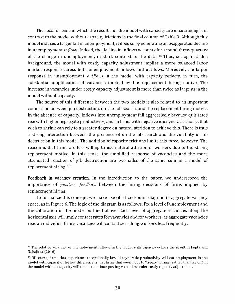
30

The second sense in which the results for the model with capacity are encouraging is in contrast to the model without capacity frictions in the final column of Table 3. Although this model induces a larger fall in unemployment, it does so by generating an exaggerated decline in unemployment inflows. Indeed, the decline in inflows accounts for around three-quarters of the change in unemployment, in stark contrast to the data.14F

15 Thus, set against this background, the model with costly capacity adjustment implies a more balanced labor market response across both unemployment inflows and outflows. Moreover, the larger response in unemployment outflows in the model with capacity reflects, in turn, the substantial amplification of vacancies implied by the replacement hiring motive. The increase in vacancies under costly capacity adjustment is more than twice as large as in the model without capacity.

The source of this difference between the two models is also related to an important connection between job destruction, on-the-job search, and the replacement hiring motive. In the absence of capacity, inflows into unemployment fall aggressively because quit rates rise with higher aggregate productivity, and so firms with negative idiosyncratic shocks that wish to shrink can rely to a greater degree on natural attrition to achieve this. There is thus a strong interaction between the presence of on-the-job search and the volatility of job destruction in this model. The addition of capacity frictions limits this force, however. The reason is that firms are less willing to use natural attrition of workers due to the strong replacement motive. In this sense, the amplified response of vacancies and the more attenuated reaction of job destruction are two sides of the same coin in a model of replacement hiring.15F

16

Feedback in vacancy creation. In the introduction to the paper, we underscored the importance of positive feedback between the hiring decisions of firms implied by replacement hiring.

To formalize this concept, we make use of a fixed-point diagram in aggregate vacancy space, as in Figure 6. The logic of the diagram is as follows. Fix a level of unemployment and the calibration of the model outlined above. Each level of aggregate vacancies along the horizontal axis will imply contact rates for vacancies and for workers: as aggregate vacancies rise, an individual firm’s vacancies will contact searching workers less frequently,

15 The relative volatility of unemployment inflows in the model with capacity echoes the result in Fujita and Nakajima (2016). 16 Of course, firms that experience exceptionally low idiosyncratic productivity will cut employment in the model with capacity. The key difference is that firms that would opt to “freeze” hiring (rather than lay off) in the model without capacity will tend to continue posting vacancies under costly capacity adjustment.

31

Figure 6. The steady-state equilibrium response of vacancies to aggregate productivity

A. Model with 𝑘𝑘 B. Model without 𝑘𝑘

and its employees will receive outside offers more frequently. Given these contact rates, firms then make their optimal vacancy-posting decisions. We plot the aggregate vacancies implied by these optimal vacancy decisions on the vertical axis. Equilibrium vacancies are thus a fixed point of this map (for a given level of unemployment, to which we shall return shortly).

Figure 6 plots this map for each of the two calibrated models—the model with capacity that captures the replacement hiring moments of section 2; and the model without capacity model that suspends this motive. The slope of the map indicates the degree of feedback in the model, that is, the degree to which vacancy posting by other firms raises a given firm’s vacancy creation.

Consider first the model without capacity in Figure 6B. Here the map is mildly upward-sloping: vacancy-posting decisions have little effect on the vacancy-posting decisions of other firms. Intuitively, this is the outcome of two opposing forces. On one hand, increased aggregate vacancies lower vacancy contact rates and raise employee quit rates. These lower desired hiring in the model, since it renders hiring more costly and jobs less durable. On the other hand, for a given level of desired hiring, a lower vacancy contact rate requires a firm to post more vacancies to achieve its desired level of hires. In the model without capacity, the latter is only slightly stronger than the former, yielding a mildly upward-sloped map, reflecting the small share of replacement hiring in our calibrated version of this model.

Now consider the model with capacity in Figure 6A. In this model, firms have a strong incentive to replace quits due to the costs of operating with slack capacity, which are reflected in the model’s ability to generate much more significant replacement hiring than its counterpart without capacity. Figure 6A reveals that this in turn is consistent with much more significant positive feedback between the vacancy decisions of firms—the vacancy map is strongly positively inclined. The reason is that the first-order effect of higher

32

aggregate vacancies in this model is to raise the quit rate from firms, which induces more vacancy posting as firms seek to replace positions vacated by quits.

Figure 6 then reveals how these differing feedback channels in turn shape the volatility of the vacancy response to a change in aggregate productivity 𝑝𝑝. This is depicted in two stages in Figure 6: First, the rise in vacancies that would emerge holding unemployment fixed (the dotted lines); and, second, the further rise in equilibrium vacancies that emerges after unemployment has fully adjusted (the dashed lines).

Holding unemployment fixed, a rise in 𝑝𝑝 shifts up the vacancy locus (to the dotted lines in Figure 6). The implied initial response of vacancies is then increasing in the degree of positive feedback, as indicated by the slope of the vacancy locus. Intuitively, initial rises in vacancies driven by aggregate expansions set off a chain reaction of further vacancy posting as firms increasingly poach workers from each other, amplifying the equilibrium response of aggregate vacancies. Because the degree of replacement hiring in the model with capacity is much larger, this initial response is much larger in that model than in the no-capacity counterpart.

As unemployment adjusts, the vacancy locus shifts up still further (to the dashed lines in Figure 6). The positive feedback that induces volatile initial equilibrium vacancy responses also amplifies the feedback effect from unemployment back onto vacancies. The intuition is analogous: As unemployment declines, the labor market tightens still further, and quit rates (and hence poaching) rise still further. This induces yet further increases in vacancy posting when there is a strong replacement hiring motive. Since the latter is much stronger in the model with capacity, the quantitative rise in vacancies from this channel is significantly stronger.

Strikingly, in the model with capacity, both of these effects are large and contribute in approximately equal measure to the volatility of equilibrium vacancies in the model. By contrast, both effects are considerably smaller in magnitude, particularly that driven by the feedback from unemployment adjustment. Thus, the additional replacement hiring driven by the putty-clay technology generates positive feedback in vacancy creation—a vacancy

chain—that contributes importantly to the responsiveness of vacancies to changes in aggregate change productivity.

33

References

Abraham, Arpad and Kirk White. 2006. “The Dynamics of Plant-level Productivity in U.S. Manufacturing.” Center for Economic Studies WP 06-20.

Acemoglu, Daron, and William Hawkins. 2014. “Search with Multi-worker Firms.” Theoretical Economics 9(3): 583–628.

Akerlof, George A., Andrew Rose, and Janet Yellen. “Job Switching and Job Satisfaction in the U.S. Labor Market.” Brookings Papers on Economic Activity 1988.2: 495-594.

Bilal, Adrien, Niklas Engbom, Simon Mongey, and Giovanni L. Violante. 2019. “Firm and Worker Dynamics in a Frictional Labor Market.” Mimeo, Princeton University.

Binmore, Ken, Ariel Rubinstein, and Asher Wolinsky. 1986. “The Nash Bargaining Solution in Economic Modeling.” RAND Journal of Economics 17: 176-188.

Bloom, Nicholas. 2009. “The Impact of Uncertainty Shocks.” Econometrica 77(3): 623-685.

Bruegemann, Bjoern, Pieter Gautier, and Guido Menzio. 2018. “Intra Firm Bargaining and Shapley Values.” Review of Economic Studies 86(2): 564-592.

Burgess, Simon, Julia Lane, and David Stevens. 2001. “Churning Dynamics: An Analysis of Hires and Separations at the Employer Level.” Labour Economics 8(1): 1-14.

Chase, Ivan D. 1991. “Vacancy Chains.” Annual Review of Sociology 17: 133-154.

Cooper, Russell, John Haltiwanger, and Jonathan L. Willis. 2007. “Search frictions: Matching aggregate and establishment observations.” Journal of Monetary Economics 54(1): 56-78.

Cooper, Russell, John Haltiwanger, and Jonathan L. Willis. 2015. “Dynamics of labor demand: Evidence from plant-level observations and aggregate implications.” Research in Economics 6(1): 37-50.

Davis, Steven J., and John Haltiwanger. 1992. “Gross Job Creation, Gross Job Destruction, and Employment Reallocation.” Quarterly Journal of Economics 107(3): 819-864.

Davis, Steven J., John Haltiwanger, and Scott Schuh. 1996. Job Creation and Destruction. MIT Press. Davis, Steven J., R. Jason Faberman and John C. Haltiwanger. 2006. “The Flow Approach to Labor Markets:

New Data Sources and Micro-Macro Links.” Journal of Economic Perspectives 20(3): 3-26.

Davis, Steven J., R. Jason Faberman and John C. Haltiwanger. 2012. “Labor Market Flows in the Cross Section and Over Time.” Journal of Monetary Economics 59(1): 1-18.

Davis, Steven J., R. Jason Faberman and John C. Haltiwanger. 2013. “The establishment-level behavior of vacancies and hiring.” Quarterly Journal of Economics 128(2): 581-622.

Eichenbaum, Martin, Nir Jaimovich, and Sergio Rebelo. 2011. “Reference Prices, Costs, and Nominal Rigidities.” American Economic Review 101: 234-262.

Elsby, Michael W. L. and Axel Gottfries. 2019. “Firm Dynamics, On-the-Job Search, and Labor Market Fluctuations.” Mimeo, University of Edinburgh.

Elsby, Michael W. L., Ryan Michaels, and Gary Solon. 2009. “The Ins and Outs of Cyclical Unemployment.” American Economic Journal: Macroeconomics 1(1): 84-110.

Elsby, Michael W. L. and Ryan Michaels. 2013. “Marginal Jobs, Heterogeneous Firms, and Unemployment Flows.” American Economic Journal: Macroeconomics 5(1): 1-48.

34

Elsby, Michael W. L., Ryan Michaels, and David Ratner. 2015. “The Beveridge Curve: A Survey.” Journal of Economic Literature 53(3): 571-630.

Elsby, Michael W. L., Gary Solon, and Donggyun Shin. 2016. “Wage Adjustment in the Great Recession and other Downturns: Evidence from the United States and Great Britain.” Journal of Labor Economics 34(1): S249-S291.

Elsby, Michael W. L., Ryan Michaels, and David Ratner. 2019. “The Aggregate Effects of Labor Market Frictions.” Quantitative Economics 10(3): 803-852.

Faberman, R. Jason and Eva Nagypal. 2008. “Quits, Worker Replacement, and Firm Growth: Theory and Evidence.” Federal Reserve Bank of Philadelphia Working Paper No. 08-13.

Fallick, Bruce, and Charles A. Fleischman. 2004. “Employer-to-Employer Flows in the U.S. Labor Market: The Complete Picture of Gross Worker Flows.” Finance and Economics Discussion Series 2004-34, Board of Governors of the Federal Reserve System.

Fallick, Bruce, John C. Haltiwanger, and Erika McEntarfer (2012). “Job-to-Job Flows and the Consequences of Job Separations.” Board of Governors of the Federal Reserve Finance and Economics Discussion Series 2012-73.

Foote, Chris. 1998. “Trend Employment Growth and the Bunching of Job Creation and Destruction.” Quarterly Journal of Economics 113(3): 809-834.

Fujita, Shigeru, and Gary Ramey. 2009. “The Cyclicality of Separation and Job Finding Rates.” International Economic Review 50(2): 415-430.

Fujita, Shigeru, and Makoto Nakajima. 2016. “Worker Flows and Job Flows: A Quantitative Investigation.” Review of Economic Dynamics, 22: 1-20

Fuss, Melyvn A. 1977. “The Structure of Technology over Time: A Model for Testing the ‘Putty-Clay’ Hypothesis.” Econometrica 45(8): 1797-1821.

Gavazza, Alessandro, Simon Mongey, and Giovanni L. Violante. 2018. “Aggregate Recruiting Intensity.” American Economic Review 108(8): 2088-2127.

Gottfries, Axel. 2019. “Bargaining with Renegotiation in Models with On-the-Job Search,” Mimeo, University of Edinburgh.

Hagedorn, Marcus and Iourii Manovskii. 2008. “The Cyclical Behavior of Unemployment, Vacancies, and Wages Revisited.” American Economic Review 98(4): 1692-1706.

Hall, Robert E. and Paul R. Milgrom. 2008. “The Limited Influence of Unemployment on the Wage Bargain.” American Economic Review 98(4): 1653-1674.

Hamermesh, Daniel. 1989. “Labor Demand and the Structure of Adjustment Costs.” American Economic Review 79(4): 674-689.

Kaas, Leo and Philipp Kircher. 2015. “Efficient Firm Dynamics in a Frictional Labor Market.” American Economic Review 105(10): 3030-3060.

Krause, Michael U. and Thomas A. Lubik. 2006. “The Cyclical Upgrading of Labor and On-the-Job Search.” Labour Economics 13(4): 459-477.

Krusell, Per and Anthony Smith. 1998. “Income and Wealth Heterogeneity in the Macroeconomy.” Journal of Political Economy 106(5): 867-896.

Lazear, Edward and James R. Spletzer. 2012. “Hiring, Churn, and the Business Cycle.” American Economic Review Papers and Proceedings 102(3): 575-579.

35

Lentz, Rasmus and Dale T. Mortensen. 2012. “Labor Market Friction, Firm Heterogeneity, and Aggregate Employment and Productivity.” Mimeo, University of Wisconsin.

Manning, Alan. 1994. “How Robust is the Theory of the Trade Union.” Journal of Labor Economics 12: 430-459.

Manning, Alan. 2011. “Imperfect Competition in the Labour Market.” Handbook of Labor Economics Vol. 4b. Elsevier.

Malcomson, J.M. and M.J. Prior. 1979. “The Estimation of a Vintage Model of Production for UK Manufacturing.” Review of Economic Studies 46: 353-369.

Mortensen, Dale T., and Christopher A. Pissarides. 1994. “Job creation and job destruction in the theory of unemployment.” Review of Economic Studies 61(3): 397-415.

Mukoyama, Toshihiko, Christina Patterson, and Ayşegül Sahin. 2018. “Job Search Behavior over the Business Cycle,” American Economic Journal: Macroeconomics 10(1): 190-215.

Nagypal, Eva. 2007. “Labor Market Fluctuations and On-the-Job Search.” Mimeo, Northwestern University.

Nickell, Stephen. 1978. “Fixed Costs, Employment and Labour Demand Over the Cycle.” Economica 45(180): 329-345.

Oi, Walter Y. “Labor as a Quasi-Fixed Factor.” Journal of Political Economy 70(6): 538-555.

Postel-Vinay, Fabien and Jean-Marc Robin. 2002. “Equilibrium Wage Dispersion with Worker and Employer Heterogeneity.” Econometrica 70(6): 2295-2350.

Rogerson, Richard, and Robert Shimer. 2011. “Search in Macroeconomic Models of the Labor Market.” Handbook of Labor Economics Vol. 4b. Elsevier.

Schaal, Edouard. 2017. “Uncertainty and Unemployment.” Econometrica 85(6): 1675-1721.

Schoefer, Benjamin and Yusuf Mercan. 2019. “Jobs and Matches: Quits, Replacement Hiring, and Vacancy Chains.” American Economic Review: Insights 2(1): 101-124.

Shimer, Robert. 2012. “Reassessing the Ins and Outs of Unemployment.” Review of Economic Dynamics 15(2): 127-148.

Shimer, Robert. 2006. “On-the-Job Search and Strategic Bargaining.” European Economic Review 50(4): 811-830.

Shimer, Robert. 2005. “The Cyclical Behavior of Equilibrium Unemployment and Vacancies.” American Economic Review 95(1): 25-49.

Silva, Jose I. and Manuel Toledo. 2009. “Labor Turnover Costs and the Cyclical Behavior of Vacancies and Unemployment.” Macroeconomic Dynamics 13(S1): 86-96.

Solon, Gary, Robert Barsky, and Jonathan Parker. 1994. “Measuring the Cyclicality of Real Wages: How Important is Composition Bias?” Quarterly Journal of Economics 109(1): 1-25.

Stole, Lars A. and Jeffrey Zwiebel. 1996. “Intrafirm Bargaining Under Non-binding Contracts.” Review of Economic Studies 63(3): 375-410.

White, Harrison C. 1970. Chains of Opportunity: System Models of Mobility in Organizations. Cambridge, Mass.: Harvard University Press.