FACULDADE DE ECONOMIA

UNIVERSIDADE DO PORTO

Faculdade de Economia do Porto - R. Dr. Roberto Frias - 4200-464 Porto - Portugal Tel . +351 225 571 100 - Fax. +351 225 505 050 - http://www.fep.up.pt

WORKING PAPERS DA FEP

AN EXACT APPROACH TO EARLY/TARDY SCHEDULING

WITH RELEASE DATES

Jorge M. S. ValenteRui A. F. S. Alves

Investigação - Trabalhos em curso - nº 129, Maio de 2003

www.fep.up.pt

An exact approach to early/tardy scheduling with

release dates

Jorge M. S. Valente and Rui A. F. S. Alves

Faculdade de Economia do Porto

Rua Dr. Roberto Frias, 4200-464 Porto, Portugal

e-mails: jvalente@fep.up.pt; ralves@fep.up.pt

May 29, 2003

Abstract

In this paper we consider the single machine earliness/tardiness scheduling problem

with different release dates and no unforced idle time. The problem is decomposed into

a weighted earliness subproblem and a weighted tardiness subproblem. Lower bounding

procedures are proposed for each of these subproblems, and the lower bound for the original

problem is then simply the sum of the lower bounds for the two subproblems. The lower

bounds and several versions of a branch-and-bound algorithm are then tested on a set of

randomly generated problems, and instances with up to 30 jobs are solved to optimality.

To the best of our knowledge, this is the first exact approach for the early/tardy scheduling

problem with release dates and no unforced idle time.

Keywords: scheduling, early/tardy, release dates, lower bounds, branch-and-bound

Resumo

Neste artigo é considerado um problema de sequenciamento com uma única máquina,

custos de posse e de atraso e datas de disponibilidade distintas no qual não é permitida

a existência de tempo morto não forçado. Este problema é decomposto num subprob-

lema weighted earliness e num subproblema weighted tardiness. Procedimentos de lower

bound são propostos para cada um destes subproblemas, e um lower bound para o prob-

lema original pode ser obtido somando os lower bounds dos dois subproblemas. Os lower

1

bounds e várias versões de um algoritmo branch-and-bound são testados num conjunto de

problemas gerado aleatoriamente, tendo instâncias com até 30 trabalhos sido resolvidas

de forma óptima.

Palavras-chave: sequenciamento, custos de posse e atraso, datas de disponibilidade,

lower bounds, branch-and-bound

1 Introduction

In this paper we consider a single machine scheduling problem with release dates

and earliness and tardiness costs that can be stated as follows. A set of n inde-

pendent jobs J1, J2, · · · , Jn has to be scheduled without preemptions on a singlemachine that can handle at most one job at a time. The machine is assumed to be

continuously available from time zero onwards and unforced machine idle time is not

allowed. Job Jj, j = 1, 2, · · · , n, becomes available for processing at its release daterj, requires a processing time pj and should ideally be completed on its due date dj.

For any given schedule, the earliness and tardiness of Jj can be respectively defined

as Ej = max 0, dj − Cj and Tj = max 0, Cj − dj, where Cj is the completion

time of Jj. The objective is then to find the schedule that minimises the sum of the

earliness and tardiness costs of all jobsPn

j=1 (hjEj + wjTj), where hj and wj are

the earliness and tardiness penalties of job Jj.

The inclusion of both earliness and tardiness costs in the objective function is

compatible with the philosophy of just-in-time production, which emphasizes pro-

ducing goods only when they are needed. The early cost may represent the cost

of completing a project early in PERT-CPM analyses, deterioration in the produc-

tion of perishable goods or a holding cost for finished goods. The tardy cost can

represent rush shipping costs, lost sales and loss of goodwill. It is assumed that no

unforced machine idle time is allowed, so the machine is only idle if no job is cur-

rently available for processing. This assumption reflects a production setting where

the cost of machine idleness is higher than the early cost incurred by completing any

job before its due date, or the capacity of the machine is limited when compared

with its demand, so that the machine must indeed be kept running. Some specific

examples of production settings with these characteristics are provided by Korman

[6] and Landis [7]. The existence of different release dates is compatible with the

assumption of no unforced idle time, as long as the forced idle time caused by the

presence of distinct release dates is small or inexistent. If that is not the case, that

2

assumption becomes unrealistic, since it is then highly unlikely that either the ma-

chine idleness cost is higher than the early cost or the machine capacity is limited

when compared with the demand.

As a generalization of weighted tardiness scheduling [8], the problem is strongly

NP-hard. To the best of our knowledge, we know of no published work on this prob-

lem. The early/tardy problemwith equal release dates and no idle time, however, has

been considered by several authors, and both exact and heuristic approaches have

been proposed. Among the exact approaches, branch-and-bound algorithms were

presented by Abdul-Razaq and Potts [1], Li [9] and Liaw [10]. The lower bounding

procedure of Abdul-Razaq and Potts was based on the subgradient optimization ap-

proach and the dynamic programming state-space relaxation technique, while Li and

Liaw used Lagrangean relaxation and the multiplier adjustment method. Among

the heuristics, Ow and Morton [11] developed several dispatch rules and a filtered

beam search procedure. Valente and Alves [12] presented an additional dispatch rule

and a greedy procedure, and also considered the use of dominance rules to further

improve the schedule obtained by the heuristics. A neighbourhood search algorithm

was also presented by Li [9]. The weighted tardiness problem with release dates

has also been considered by Akturk and Ozdemir ([3], [2]). In [3] they present a

dominance rule that is used as an improvement step after a dispatch heuristic has

generated an initial schedule, and is also implemented in two local search heuristics,

in order to guide them to the areas that will most likely contain the good solu-

tions. In [2], Akturk and Ozdemir present some new dominance rules and two lower

bounding procedures that are incorporated in a branch-and-bound algorithm.

In this paper we present a branch-and-bound algorithm based on a decomposi-

tion of the problem into a weighted earliness subproblem and a weighted tardiness

subproblem. We propose lower bound procedures for each of these subproblems, and

the lower bound for the original problem is then simply the sum of the lower bounds

for the two subproblems. We also propose using two dominance rules originally de-

rived for the problem with equal release dates in order to eliminate dominated nodes

from the search tree. These rules can still be used in the presence of release dates

provided a slight adjustment is made. Several versions of the branch-and-bound

algorithm are then tested on a set of randomly generated problems with up to 30

jobs.

This paper is organized as follows. In section 2 we describe the decomposition

of the problem and the derivation of the lower bound procedures. The dominance

3

rules are presented in section 3. Section 4 describes the implementation details of the

branch-and-bound algorithm. The computational results are presented in section 5.

Finally, conclusions are provided in section 6.

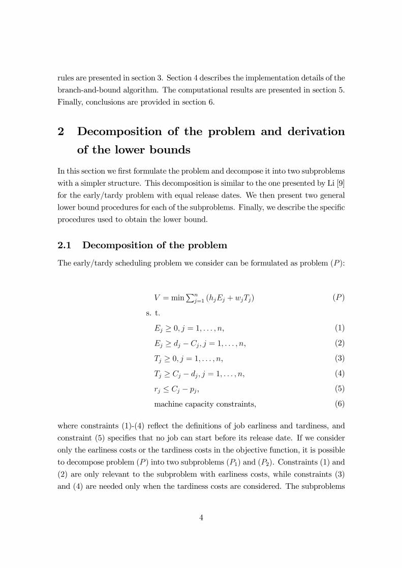
2 Decomposition of the problem and derivation

of the lower bounds

In this section we first formulate the problem and decompose it into two subproblems

with a simpler structure. This decomposition is similar to the one presented by Li [9]

for the early/tardy problem with equal release dates. We then present two general

lower bound procedures for each of the subproblems. Finally, we describe the specific

procedures used to obtain the lower bound.

2.1 Decomposition of the problem

The early/tardy scheduling problem we consider can be formulated as problem (P ):

V = minPn

j=1 (hjEj + wjTj) (P )

s. t.

Ej ≥ 0, j = 1, . . . , n, (1)

Ej ≥ dj − Cj, j = 1, . . . , n, (2)

Tj ≥ 0, j = 1, . . . , n, (3)

Tj ≥ Cj − dj, j = 1, . . . , n, (4)

rj ≤ Cj − pj, (5)

machine capacity constraints, (6)

where constraints (1)-(4) reflect the definitions of job earliness and tardiness, and

constraint (5) specifies that no job can start before its release date. If we consider

only the earliness costs or the tardiness costs in the objective function, it is possible

to decompose problem (P ) into two subproblems (P1) and (P2). Constraints (1) and

(2) are only relevant to the subproblem with earliness costs, while constraints (3)

and (4) are needed only when the tardiness costs are considered. The subproblems

4

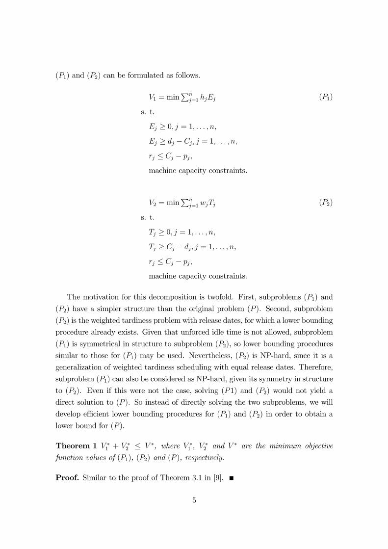
(P1) and (P2) can be formulated as follows.

V1 = minPn

j=1 hjEj (P1)

s. t.

Ej ≥ 0, j = 1, . . . , n,Ej ≥ dj − Cj, j = 1, . . . , n,

rj ≤ Cj − pj,

machine capacity constraints.

V2 = minPn

j=1wjTj (P2)

s. t.

Tj ≥ 0, j = 1, . . . , n,Tj ≥ Cj − dj, j = 1, . . . , n,

rj ≤ Cj − pj,

machine capacity constraints.

The motivation for this decomposition is twofold. First, subproblems (P1) and

(P2) have a simpler structure than the original problem (P ). Second, subproblem

(P2) is the weighted tardiness problem with release dates, for which a lower bounding

procedure already exists. Given that unforced idle time is not allowed, subproblem

(P1) is symmetrical in structure to subproblem (P2), so lower bounding procedures

similar to those for (P1) may be used. Nevertheless, (P2) is NP-hard, since it is a

generalization of weighted tardiness scheduling with equal release dates. Therefore,

subproblem (P1) can also be considered as NP-hard, given its symmetry in structure

to (P2). Even if this were not the case, solving (P1) and (P2) would not yield a

direct solution to (P ). So instead of directly solving the two subproblems, we will

develop efficient lower bounding procedures for (P1) and (P2) in order to obtain a

lower bound for (P ).

Theorem 1 V ∗1 + V ∗2 ≤ V ∗, where V ∗1 , V∗2 and V ∗ are the minimum objective

function values of (P1), (P2) and (P ), respectively.

Proof. Similar to the proof of Theorem 3.1 in [9].

5

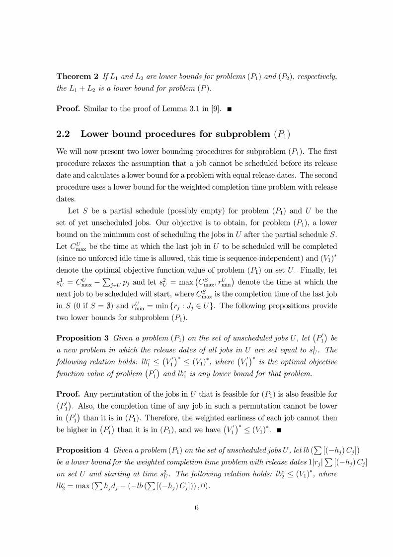
Theorem 2 If L1 and L2 are lower bounds for problems (P1) and (P2), respectively,the L1 + L2 is a lower bound for problem (P ).

Proof. Similar to the proof of Lemma 3.1 in [9].

2.2 Lower bound procedures for subproblem (P1)

We will now present two lower bounding procedures for subproblem (P1). The first

procedure relaxes the assumption that a job cannot be scheduled before its release

date and calculates a lower bound for a problem with equal release dates. The second

procedure uses a lower bound for the weighted completion time problem with release

dates.

Let S be a partial schedule (possibly empty) for problem (P1) and U be the

set of yet unscheduled jobs. Our objective is to obtain, for problem (P1), a lower

bound on the minimum cost of scheduling the jobs in U after the partial schedule S.

Let CUmax be the time at which the last job in U to be scheduled will be completed

(since no unforced idle time is allowed, this time is sequence-independent) and (V1)∗

denote the optimal objective function value of problem (P1) on set U . Finally, let

s1U = CUmax −

Pj∈U pj and let s2U = max

¡CSmax, r

Umin

¢denote the time at which the

next job to be scheduled will start, where CSmax is the completion time of the last job

in S (0 if S = ∅) and rUmin = min rj : Jj ∈ U. The following propositions providetwo lower bounds for subproblem (P1).

Proposition 3 Given a problem (P1) on the set of unscheduled jobs U , let¡P

01

¢be

a new problem in which the release dates of all jobs in U are set equal to s1U . The

following relation holds: lbe1 ≤¡V

01

¢∗ ≤ (V1)∗, where ¡V 01

¢∗is the optimal objective

function value of problem¡P

01

¢and lbe1 is any lower bound for that problem.

Proof. Any permutation of the jobs in U that is feasible for (P1) is also feasible for¡P

01

¢. Also, the completion time of any job in such a permutation cannot be lower

in¡P

01

¢than it is in (P1). Therefore, the weighted earliness of each job cannot then

be higher in¡P

01

¢than it is in (P1), and we have

¡V

01

¢∗ ≤ (V1)∗.Proposition 4 Given a problem (P1) on the set of unscheduled jobs U , let lb (

P[(−hj)Cj])

be a lower bound for the weighted completion time problem with release dates 1|rj|P[(−hj)Cj]

on set U and starting at time s2U . The following relation holds: lbe2 ≤ (V1)∗, where

lbe2 = max (P

hjdj − (−lb (P[(−hj)Cj])) , 0).

6

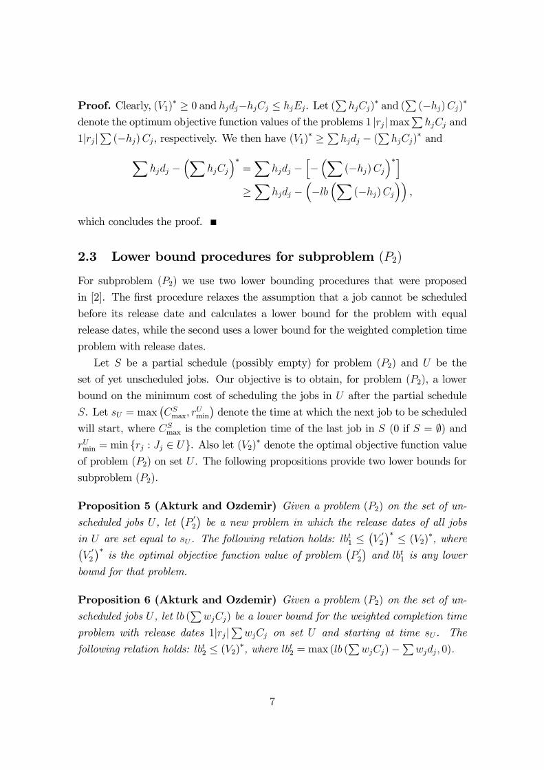
Proof. Clearly, (V1)∗ ≥ 0 and hjdj−hjCj ≤ hjEj. Let (

PhjCj)

∗ and (P(−hj)Cj)

∗

denote the optimum objective function values of the problems 1 |rj|maxP

hjCj and

1|rj|P(−hj)Cj, respectively. We then have (V1)

∗ ≥Phjdj − (P

hjCj)∗ andX

hjdj −³X

hjCj

´∗=X

hjdj −h−³X

(−hj)Cj

´∗i≥X

hjdj −³−lb

³X(−hj)Cj

´´,

which concludes the proof.

2.3 Lower bound procedures for subproblem (P2)

For subproblem (P2) we use two lower bounding procedures that were proposed

in [2]. The first procedure relaxes the assumption that a job cannot be scheduled

before its release date and calculates a lower bound for the problem with equal

release dates, while the second uses a lower bound for the weighted completion time

problem with release dates.

Let S be a partial schedule (possibly empty) for problem (P2) and U be the

set of yet unscheduled jobs. Our objective is to obtain, for problem (P2), a lower

bound on the minimum cost of scheduling the jobs in U after the partial schedule

S. Let sU = max¡CSmax, r

Umin

¢denote the time at which the next job to be scheduled

will start, where CSmax is the completion time of the last job in S (0 if S = ∅) and

rUmin = min rj : Jj ∈ U. Also let (V2)∗ denote the optimal objective function valueof problem (P2) on set U . The following propositions provide two lower bounds for

subproblem (P2).

Proposition 5 (Akturk and Ozdemir) Given a problem (P2) on the set of un-

scheduled jobs U , let¡P

02

¢be a new problem in which the release dates of all jobs

in U are set equal to sU . The following relation holds: lbt1 ≤¡V

02

¢∗ ≤ (V2)∗, where¡V

02

¢∗is the optimal objective function value of problem

¡P

02

¢and lbt1 is any lower

bound for that problem.

Proposition 6 (Akturk and Ozdemir) Given a problem (P2) on the set of un-

scheduled jobs U , let lb (P

wjCj) be a lower bound for the weighted completion time

problem with release dates 1|rj|P

wjCj on set U and starting at time sU . The

following relation holds: lbt2 ≤ (V2)∗, where lbt2 = max (lb (P

wjCj)−P

wjdj, 0).

7

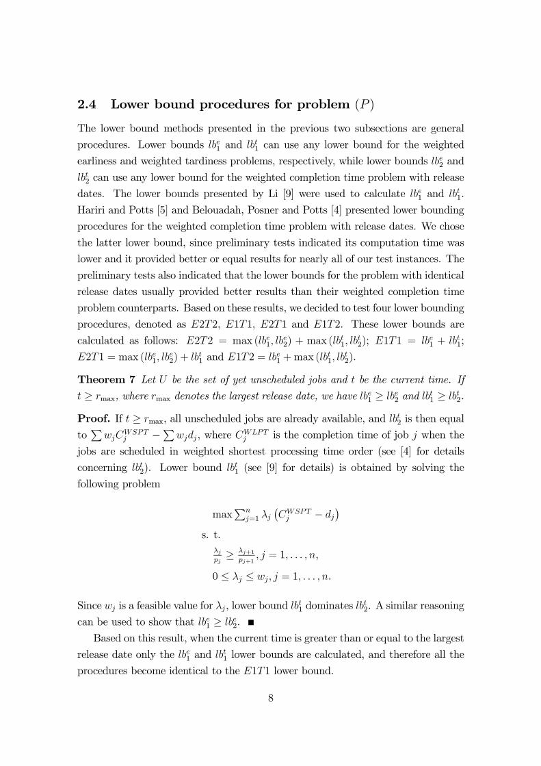
2.4 Lower bound procedures for problem (P )

The lower bound methods presented in the previous two subsections are general

procedures. Lower bounds lbe1 and lbt1 can use any lower bound for the weighted

earliness and weighted tardiness problems, respectively, while lower bounds lbe2 and

lbt2 can use any lower bound for the weighted completion time problem with release

dates. The lower bounds presented by Li [9] were used to calculate lbe1 and lbt1.

Hariri and Potts [5] and Belouadah, Posner and Potts [4] presented lower bounding

procedures for the weighted completion time problem with release dates. We chose

the latter lower bound, since preliminary tests indicated its computation time was

lower and it provided better or equal results for nearly all of our test instances. The

preliminary tests also indicated that the lower bounds for the problem with identical

release dates usually provided better results than their weighted completion time

problem counterparts. Based on these results, we decided to test four lower bounding

procedures, denoted as E2T2, E1T1, E2T1 and E1T2. These lower bounds are

calculated as follows: E2T2 = max (lbe1, lbe2) + max (lb

t1, lb

t2); E1T1 = lbe1 + lbt1;

E2T1 = max (lbe1, lbe2) + lbt1 and E1T2 = lbe1 +max (lb

t1, lb

t2).

Theorem 7 Let U be the set of yet unscheduled jobs and t be the current time. If

t ≥ rmax, where rmax denotes the largest release date, we have lbe1 ≥ lbe2 and lbt1 ≥ lbt2.

Proof. If t ≥ rmax, all unscheduled jobs are already available, and lbt2 is then equal

toP

wjCWSPTj −Pwjdj, where CWLPT

j is the completion time of job j when the

jobs are scheduled in weighted shortest processing time order (see [4] for details

concerning lbt2). Lower bound lbt1 (see [9] for details) is obtained by solving the

following problem

maxPn

j=1 λj¡CWSPTj − dj

¢s. t.

λjpj≥ λj+1

pj+1, j = 1, . . . , n,

0 ≤ λj ≤ wj, j = 1, . . . , n.

Since wj is a feasible value for λj, lower bound lbt1 dominates lbt2. A similar reasoning

can be used to show that lbe1 ≥ lbe2.

Based on this result, when the current time is greater than or equal to the largest

release date only the lbe1 and lbt1 lower bounds are calculated, and therefore all the

procedures become identical to the E1T1 lower bound.

8

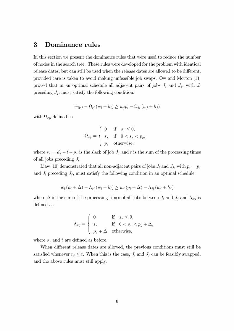
3 Dominance rules

In this section we present the dominance rules that were used to reduce the number

of nodes in the search tree. These rules were developed for the problem with identical

release dates, but can still be used when the release dates are allowed to be different,

provided care is taken to avoid making unfeasible job swaps. Ow and Morton [11]

proved that in an optimal schedule all adjacent pairs of jobs Ji and Jj, with Ji

preceding Jj, must satisfy the following condition:

wipj − Ωij (wi + hi) ≥ wjpi − Ωji (wj + hj)

with Ωxy defined as

Ωxy =

0 if sx ≤ 0,sx if 0 < sx < py,

py otherwise,

where sx = dx− t− px is the slack of job Jx and t is the sum of the processing times

of all jobs preceding Ji.

Liaw [10] demonstrated that all non-adjacent pairs of jobs Ji and Jj, with pi = pj

and Ji preceding Jj, must satisfy the following condition in an optimal schedule:

wi (pj +∆)− Λij (wi + hi) ≥ wj (pi +∆)− Λji (wj + hj)

where ∆ is the sum of the processing times of all jobs between Ji and Jj and Λxy is

defined as

Λxy =

0 if sx ≤ 0,sx if 0 < sx < py +∆,

py +∆ otherwise,

where sx and t are defined as before.

When different release dates are allowed, the previous conditions must still be

satisfied whenever rj ≤ t. When this is the case, Ji and Jj can be feasibly swapped,

and the above rules must still apply.

9

4 Implementation of the branch-and-bound algo-

rithm

In this section we briefly discuss the implementation of the branch-and-bound al-

gorithm. We first calculate an upper bound on the optimum schedule cost. The

EXP-ET dispatch rule originally developed in [11] for the problem with identical

release dates is used to generate an initial sequence. The dominance rules described

in the previous section are then applied to improve this sequence. First, the adjacent

dominance rule of Ow and Morton is used. When a pair of adjacent jobs violates

that rule, those jobs are swapped. This procedure is repeated until no improvement

is found by the adjacent rule in a complete iteration. Then Liaw’s non-adjacent rule

is applied. Once again, if a pair of jobs violates the rule those jobs are swapped,

and the procedure is repeated until no improvement is made in a complete iteration.

The above two steps are repeated while the number of iterations performed by the

non-adjacent rule is greater than one (i.e., while that rule detects an improvement).

The upper bound value is updated whenever a feasible schedule with a lower cost is

found during the branching process.

We use a forward-sequencing branching rule, where a node at level l of the search

tree corresponds to a sequence with l jobs fixed in the first l positions. The depth-

first strategy is used to search the tree, and ties are broken by selecting the node

with the smallest value of the associated partial schedule cost plus the associated

lower bound for the unscheduled jobs. We also use some tests to decide whether a

node should be discarded or not. In one version of the branch-and-bound algorithm,

three tests are used. In the first test, the adjacent dominance rule of Ow and Morton

is applied to the two jobs most recently added to the node’s partial schedule. In the

second test, Liaw’s non-adjacent rule is applied. Finally, if the node is not eliminated

by the two previous tests, a lower bound is calculated for that node. If the lower

bound plus the cost of the associated partial schedule is larger than or equal to

the current upper bound, the node is discarded. The non-adjacent rule is of more

limited applicability, since it applies only to jobs with identical processing times,

and the existence of different release dates can further limit its use. Therefore, we

decided to test another version of the branch-and-bound algorithm that does not use

the non adjacent rule, and only applies the other two tests. The branch-and-bound

algorithms will be identified by the lower bound used, followed by "+N" when the

non-adjacent rule dominance test is applied.

10

5 Computational results

In this section we present the results from the computational tests. A set of problems

with 15, 20, 25, 30, 40, 50, 75, 100, 250, 500 and 1000 jobs was randomly generated

as follows. For each job Jj an integer processing time pj, an integer earliness penalty

hj and an integer tardiness penalty wj were generated from one of the two uniform

distributions [1, 10] and [1, 100], to create low and high variability, respectively. For

each job Jj, an integer release date rj was generated from the uniform distributionh0, α

Pnj=1 pj

i, where α was set at 0.25, 0.50 and 0.75. The maximum value of the

range of release dates α was chosen so that the forced idle time would be small

or inexistent. Preliminary tests showed that a higher value of 1.00 would lead

to excessive amounts of forced idle time, which would be incompatible with the

assumption that no unforced idle time may be inserted in a schedule. Instead of

determining due dates directly, we generated slack times between a job’s due date

and its earliest possible completion time. For each job Jj, an integer due date

slack sdj was generated from the uniform distributionh0, β

Pnj=1 pj

i, where the due

date slack range β was set at 0.10, 0.25 and 0.50. The due date dj of Jj was then

set equal to dj = (rj + pj) + sdj . The values considered for each of the factors

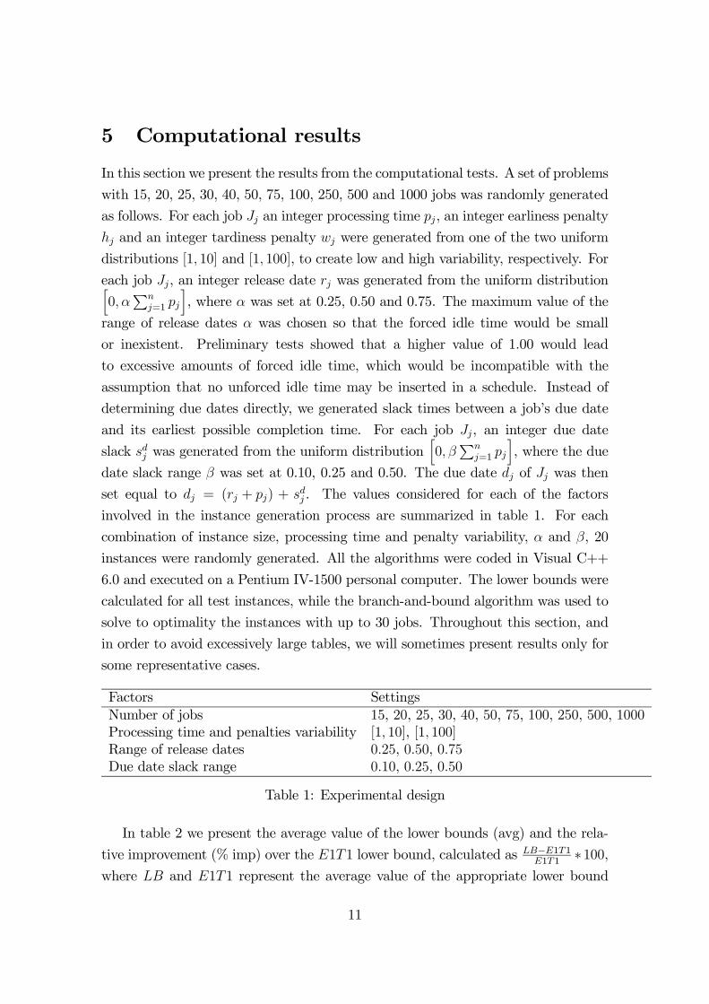
involved in the instance generation process are summarized in table 1. For each

combination of instance size, processing time and penalty variability, α and β, 20

instances were randomly generated. All the algorithms were coded in Visual C++

6.0 and executed on a Pentium IV-1500 personal computer. The lower bounds were

calculated for all test instances, while the branch-and-bound algorithm was used to

solve to optimality the instances with up to 30 jobs. Throughout this section, and

in order to avoid excessively large tables, we will sometimes present results only for

some representative cases.

Factors SettingsNumber of jobs 15, 20, 25, 30, 40, 50, 75, 100, 250, 500, 1000Processing time and penalties variability [1, 10], [1, 100]Range of release dates 0.25, 0.50, 0.75Due date slack range 0.10, 0.25, 0.50

Table 1: Experimental design

In table 2 we present the average value of the lower bounds (avg) and the rela-

tive improvement (% imp) over the E1T1 lower bound, calculated as LB−E1T1E1T1

∗100,where LB and E1T1 represent the average value of the appropriate lower bound

11

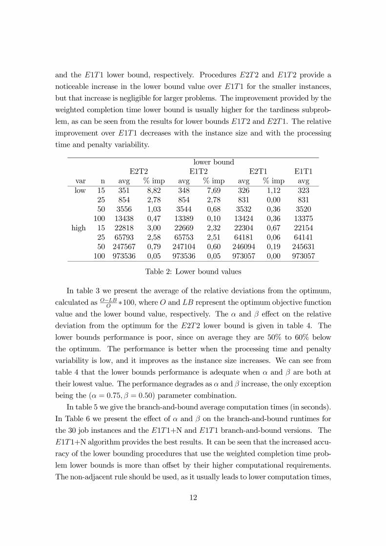
and the E1T1 lower bound, respectively. Procedures E2T2 and E1T2 provide a

noticeable increase in the lower bound value over E1T1 for the smaller instances,

but that increase is negligible for larger problems. The improvement provided by the

weighted completion time lower bound is usually higher for the tardiness subprob-

lem, as can be seen from the results for lower bounds E1T2 and E2T1. The relative

improvement over E1T1 decreases with the instance size and with the processing

time and penalty variability.

lower boundE2T2 E1T2 E2T1 E1T1

var n avg % imp avg % imp avg % imp avglow 15 351 8,82 348 7,69 326 1,12 323

25 854 2,78 854 2,78 831 0,00 83150 3556 1,03 3544 0,68 3532 0,36 3520100 13438 0,47 13389 0,10 13424 0,36 13375

high 15 22818 3,00 22669 2,32 22304 0,67 2215425 65793 2,58 65753 2,51 64181 0,06 6414150 247567 0,79 247104 0,60 246094 0,19 245631100 973536 0,05 973536 0,05 973057 0,00 973057

Table 2: Lower bound values

In table 3 we present the average of the relative deviations from the optimum,

calculated as O−LBO∗100, where O and LB represent the optimum objective function

value and the lower bound value, respectively. The α and β effect on the relative

deviation from the optimum for the E2T2 lower bound is given in table 4. The

lower bounds performance is poor, since on average they are 50% to 60% below

the optimum. The performance is better when the processing time and penalty

variability is low, and it improves as the instance size increases. We can see from

table 4 that the lower bounds performance is adequate when α and β are both at

their lowest value. The performance degrades as α and β increase, the only exception

being the (α = 0.75, β = 0.50) parameter combination.

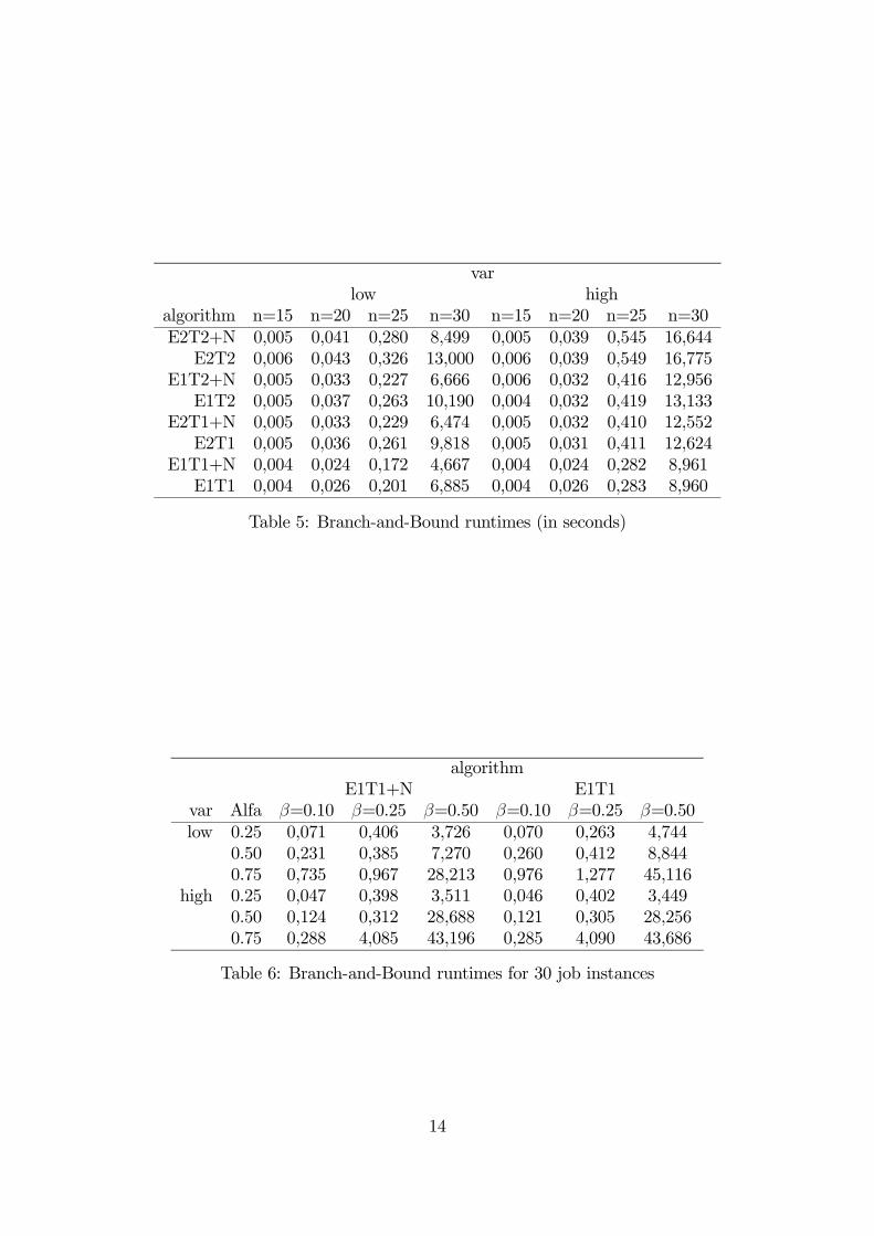
In table 5 we give the branch-and-bound average computation times (in seconds).

In Table 6 we present the effect of α and β on the branch-and-bound runtimes for

the 30 job instances and the E1T1+N and E1T1 branch-and-bound versions. The

E1T1+N algorithm provides the best results. It can be seen that the increased accu-

racy of the lower bounding procedures that use the weighted completion time prob-

lem lower bounds is more than offset by their higher computational requirements.

The non-adjacent rule should be used, as it usually leads to lower computation times,

12

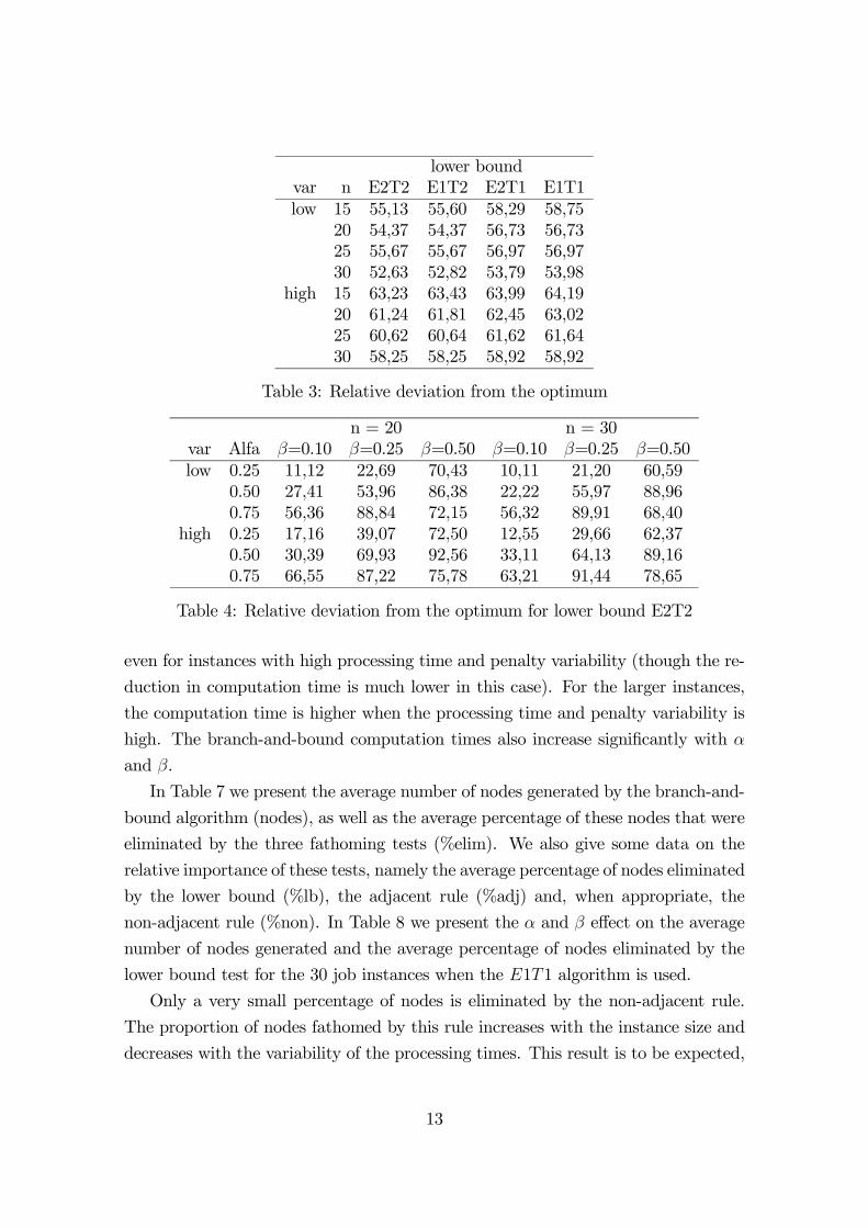
lower boundvar n E2T2 E1T2 E2T1 E1T1low 15 55,13 55,60 58,29 58,75

20 54,37 54,37 56,73 56,7325 55,67 55,67 56,97 56,9730 52,63 52,82 53,79 53,98

high 15 63,23 63,43 63,99 64,1920 61,24 61,81 62,45 63,0225 60,62 60,64 61,62 61,6430 58,25 58,25 58,92 58,92

Table 3: Relative deviation from the optimum

n = 20 n = 30var Alfa β=0.10 β=0.25 β=0.50 β=0.10 β=0.25 β=0.50low 0.25 11,12 22,69 70,43 10,11 21,20 60,59

0.50 27,41 53,96 86,38 22,22 55,97 88,960.75 56,36 88,84 72,15 56,32 89,91 68,40

high 0.25 17,16 39,07 72,50 12,55 29,66 62,370.50 30,39 69,93 92,56 33,11 64,13 89,160.75 66,55 87,22 75,78 63,21 91,44 78,65

Table 4: Relative deviation from the optimum for lower bound E2T2

even for instances with high processing time and penalty variability (though the re-

duction in computation time is much lower in this case). For the larger instances,

the computation time is higher when the processing time and penalty variability is

high. The branch-and-bound computation times also increase significantly with α

and β.

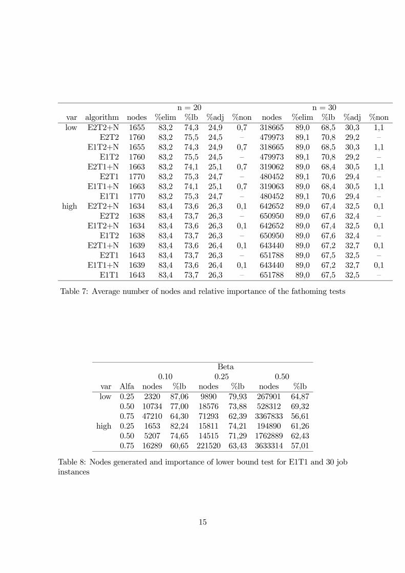
In Table 7 we present the average number of nodes generated by the branch-and-

bound algorithm (nodes), as well as the average percentage of these nodes that were

eliminated by the three fathoming tests (%elim). We also give some data on the

relative importance of these tests, namely the average percentage of nodes eliminated

by the lower bound (%lb), the adjacent rule (%adj) and, when appropriate, the

non-adjacent rule (%non). In Table 8 we present the α and β effect on the average

number of nodes generated and the average percentage of nodes eliminated by the

lower bound test for the 30 job instances when the E1T1 algorithm is used.

Only a very small percentage of nodes is eliminated by the non-adjacent rule.

The proportion of nodes fathomed by this rule increases with the instance size and

decreases with the variability of the processing times. This result is to be expected,

13

varlow high

algorithm n=15 n=20 n=25 n=30 n=15 n=20 n=25 n=30E2T2+N 0,005 0,041 0,280 8,499 0,005 0,039 0,545 16,644E2T2 0,006 0,043 0,326 13,000 0,006 0,039 0,549 16,775

E1T2+N 0,005 0,033 0,227 6,666 0,006 0,032 0,416 12,956E1T2 0,005 0,037 0,263 10,190 0,004 0,032 0,419 13,133

E2T1+N 0,005 0,033 0,229 6,474 0,005 0,032 0,410 12,552E2T1 0,005 0,036 0,261 9,818 0,005 0,031 0,411 12,624

E1T1+N 0,004 0,024 0,172 4,667 0,004 0,024 0,282 8,961E1T1 0,004 0,026 0,201 6,885 0,004 0,026 0,283 8,960

Table 5: Branch-and-Bound runtimes (in seconds)

algorithmE1T1+N E1T1

var Alfa β=0.10 β=0.25 β=0.50 β=0.10 β=0.25 β=0.50low 0.25 0,071 0,406 3,726 0,070 0,263 4,744

0.50 0,231 0,385 7,270 0,260 0,412 8,8440.75 0,735 0,967 28,213 0,976 1,277 45,116

high 0.25 0,047 0,398 3,511 0,046 0,402 3,4490.50 0,124 0,312 28,688 0,121 0,305 28,2560.75 0,288 4,085 43,196 0,285 4,090 43,686

Table 6: Branch-and-Bound runtimes for 30 job instances

14

n = 20 n = 30var algorithm nodes %elim %lb %adj %non nodes %elim %lb %adj %nonlow E2T2+N 1655 83,2 74,3 24,9 0,7 318665 89,0 68,5 30,3 1,1

E2T2 1760 83,2 75,5 24,5 — 479973 89,1 70,8 29,2 —E1T2+N 1655 83,2 74,3 24,9 0,7 318665 89,0 68,5 30,3 1,1E1T2 1760 83,2 75,5 24,5 — 479973 89,1 70,8 29,2 —

E2T1+N 1663 83,2 74,1 25,1 0,7 319062 89,0 68,4 30,5 1,1E2T1 1770 83,2 75,3 24,7 — 480452 89,1 70,6 29,4 —

E1T1+N 1663 83,2 74,1 25,1 0,7 319063 89,0 68,4 30,5 1,1E1T1 1770 83,2 75,3 24,7 — 480452 89,1 70,6 29,4 —

high E2T2+N 1634 83,4 73,6 26,3 0,1 642652 89,0 67,4 32,5 0,1E2T2 1638 83,4 73,7 26,3 — 650950 89,0 67,6 32,4 —

E1T2+N 1634 83,4 73,6 26,3 0,1 642652 89,0 67,4 32,5 0,1E1T2 1638 83,4 73,7 26,3 — 650950 89,0 67,6 32,4 —

E2T1+N 1639 83,4 73,6 26,4 0,1 643440 89,0 67,2 32,7 0,1E2T1 1643 83,4 73,7 26,3 — 651788 89,0 67,5 32,5 —

E1T1+N 1639 83,4 73,6 26,4 0,1 643440 89,0 67,2 32,7 0,1E1T1 1643 83,4 73,7 26,3 — 651788 89,0 67,5 32,5 —

Table 7: Average number of nodes and relative importance of the fathoming tests

Beta0.10 0.25 0.50

var Alfa nodes %lb nodes %lb nodes %lblow 0.25 2320 87,06 9890 79,93 267901 64,87

0.50 10734 77,00 18576 73,88 528312 69,320.75 47210 64,30 71293 62,39 3367833 56,61

high 0.25 1653 82,24 15811 74,21 194890 61,260.50 5207 74,65 14515 71,29 1762889 62,430.75 16289 60,65 221520 63,43 3633314 57,01

Table 8: Nodes generated and importance of lower bound test for E1T1 and 30 jobinstances

15

since it’s more likely to find two jobs with the same processing time when the number

of jobs is high and the variability of the processing times is low. As the instance size

and the processing time and penalty variability increase, the percentage of nodes

fathomed by the adjacent rule tends to increase, and the effectiveness of the lower

bound test correspondingly decreases. For the larger instances, the number of nodes

generated is much higher when the processing time and penalty variability is high.

The number of nodes generated also increases with α and β. The proportion of

nodes eliminated by the lower bound test usually decreases as α and β increase,

and the importance of the adjacent rule becomes correspondingly higher, since even

when the non-adjacent rule is used, it only has a marginal effect.

6 Conclusion

In this paper we considered the single machine earliness/tardiness scheduling prob-

lem with different release dates and no unforced idle time. This problem was de-

composed into weighted earliness and weighted tardiness subproblems, and lower

bounding procedures were presented for each of these subproblems. A lower bound

for the original problem is then simply the sum of the lower bounds for the two

subproblems. We also proposed using two dominance rules originally derived for the

problem with equal release dates in order to eliminate dominated nodes from the

search tree. These rules can still be used in the presence of release dates provided a

slight adjustment is made. The lower bounds and several versions of a branch-and-

bound algorithm were tested on a set of randomly generated problems, and instances

with up to 30 jobs were solved to optimality.

References

[1] Abdul-Razaq, T., and Potts, C. N. Dynamic programming state-space

relaxation for single machine scheduling. Journal of the Operational Research

Society 39 (1988), 141—152.

[2] Akturk, M. S., and Ozdemir, D. An exact approach to minimizing total

weighted tardiness with release dates. IIE Transactions 32 (2000), 1091—1101.

16

[3] Akturk, M. S., and Ozdemir, D. A new dominance rule to minimize total

weighted tardiness with unequal release dates. European Journal of Operational

Research 135 (2001), 394—412.

[4] Belouadah, H., Posner, M. E., and Potts, C. N. Scheduling with release

dates on a single machine to minimize total weighted completion time. Discrete

Applied Mathematics 36 (1992), 213—231.

[5] Hariri, A. M. A., and Potts, C. N. An algorithm for single machine

sequencing with release dates to minimize total weighted completion time. Dis-

crete Applied Mathematics 5 (1983), 99—109.

[6] Korman, K. A pressing matter. Video (February 1994), 46—50.

[7] Landis, K. Group technology and cellular manufacturing in the westvaco

los angeles vh department. Project report in iom 581, School of Business,

University of Southern California, 1993.

[8] Lenstra, J. K., Rinnooy Kan, A. H. G., and Brucker, P. Complexity

of machine scheduling problems. Annals of Discrete Mathematics 1 (1977),

343—362.

[9] Li, G. Single machine earliness and tardiness scheduling. European Journal of

Operational Research 96 (1997), 546—558.

[10] Liaw, C.-F. A branch-and-bound algorithm for the single machine earliness

and tardiness scheduling problem. Computers & Operations Research 26 (1999),

679—693.

[11] Ow, P. S., and Morton, E. T. The single machine early/tardy problem.

Management Science 35 (1989), 177—191.

[12] Valente, J. M. S., and Alves, R. A. F. S. Improved heuristics for the

early/tardy scheduling problem with no idle time. Working Paper 126, Facul-

dade de Economia do Porto, Portugal, 2003.

17