Working Paper · To achieve our target, we adopted the same strategy used by Ferreira and Gyourko (2009) for US cities, a regression discontinuity design (RDD)

CENTER FOR APPLIED MICROECONOMICS

Paulo ArvateSergio FirpoRenan Pieri

1/2014

WWoorrkkiinngg PPaappeerr

Gender stereotypes in politics: What changes when a woman becomes the local political leader?

Jan2014

priscilla.tavares

Typewritten Text

priscilla.tavares

Typewritten Text

1

Gender stereotypes in politics: What changes when a woman

becomes the local political leader?

Paulo Arvate Getulio Vargas Foundation, School of Business and Center for Applied Microeconomics (C-Micro)

Sergio Firpo Getulio Vargas Foundation, São Paulo School of Economics and C-Micro

Renan Pieri Getulio Vargas Foundation, São Paulo School of Economics and C-Micro

Abstract

This study documents how the presence of a woman in an executive political role affects the gender stereotype of women in politics. We use Brazilian electoral data and restrict our focus to close mayoral races (using an RDD design) in which the top two candidates are of opposite sexes. Our most important result was a reduction in the number of candidates and votes for female mayoral candidates after a woman is elected, regardless of her eligibility status for reelection. This negative result is linked only to the position of mayor and not to other political positions (councilor, state or federal deputy). In addition, our results may be interpreted as evidence that voters do not use their update on women as local leaders to change their beliefs on women’s ability to run for other political positions. Finally, female mayors do not appear to have a role model effect on younger cohorts of women. We also note that our results are not influenced by differences in mayoral policies (generally and specifically for women), which could influence voters’ gender stereotypes.

JEL CODE:

Keywords: Female local leaders; Gender stereotypes; Close mayoral election races.

This work received financial support from the World Bank under the project “Gender and Agency in Brazil: The Impacts of Female Local Leaders.” We benefited from comments by Fernanda Brollo, Elizaveta Perova, Johanna Karin Rickne (Research Institute for Industrial Economics), Sarah Reynolds and participants at the workshop on Chronic Poverty and Gender and Agency in the World Bank headquarters and the participants of the 2013 Midwest Political Science Association (the title of the work presented was “Discrimination in Politics, Role Model Effects, and Empowerment: What Changes When a Woman Becomes the Local Political Leader?”).

2

1. Introduction

Women’s low participation rate in politics compared to their male counterparts is partially explained

by gender stereotyping in the electorate. Recent studies indicate that exogenously increasing

constituents’ exposure to female leaders helps to increase voter support for female candidates in the

subsequent elections and the number of women participating as candidates.1 The basic argument

supporting these findings, which can be generalized as the participation of minorities in politics, is

that the negative stereotyping of minorities changes as leaders of these groups become leaders or

prominent figures in society (Sambomatsu, 2002).

These studies, however, investigate the effect of exposure, measured as tenure in office, on

changes in voters’ stereotyping of women as local leaders. Therefore, the effect described in these

studies is how exposure changes a female politician’s chances of seeking and winning the same local

position.2 Although the establishment of local female leadership is relevant in rooting new beliefs

about women’s role in overall politics, the previous literature has overlooked the effect of exposure

on female politicians beyond the local arena. Career progress in politics in general and for women in

particular is nonetheless an important topic. For example, Lawless and Theriault (2009) suggest that

one factor that induces women’s early retirement in politics is a lack of prospects, as it is much more

difficult for women than men to obtain relevant positions.

Moreover, exposure itself will only have a positive effect if the electorate positively updates

its beliefs regarding women’s abilities as politicians. Policies implemented by female politicians in

office may be intrinsically different from those implemented by their male counterparts. When

considering the total exposure effect on electoral outcomes, it becomes particularly difficult to

disentangle what is caused by differences in policies from what is caused by updates in beliefs. For

1 See Beaman, Chattopadhyay, Duflo and Topalova (2009); Bhavnani (2009); and Ferreira and Gyourko (2009). 2 Ferreira and Gyourko (2009) for mayors and Beaman, Chattopadhyay, Duflo and Topalova (2009) and Bhavnami (2009) for members of councils

3

example, an increase in the re-election chances of a local female politician might not be the result of

the electorate’s updated beliefs on women’s abilities to lead but, rather, may simply reflect an

electoral reward for the politician who was able to alter the range of policy options.

Our goal in this paper is to evaluate the impact of exogenous exposure to a local female

leader on the electorate’s gender stereotyping, controlling for differences in policies. The questions

posed are as follows: (i) Do votes for female politicians in any election (local vs. non-local, executive

vs. legislative) increase in the years after a woman has been “randomly” elected to the local executive

branch? (ii) Do elected women implement changes in policies that are intrinsically different from

what they would have been had a male politician won local elections?

We also pose the following question, which can be viewed as a control for the effectiveness

of changes in the behavior of a portion of the electorate: (iii) Is exposure to female leaders related to

an increase in young women’s engagement in politics or to changes in young women’s perceptions

of their role in society? Although this is an interesting question in itself, we use this question in our

study as a robustness check for the increased role that female leaders have been playing in the local

political arena.

We answer these questions using data from local Brazilian elections over the past 20 years.

Local Brazilian governments provide an interesting institutional setting for testing the different

effects of elected women. The executive branch of local government enjoys relative autonomy in

establishing its own public policies (Samuels, 1997).3 Because the majority of the nearly 5,600

Brazilian municipalities are relatively small (with a median size of 20,000 inhabitants; a larger number

of observations, which allows us to obtain robust empirical effects), mayors occupy a very important

3 Unlike Indian sub-national governments, for instance, local governments with executive and legislative branches function like “little countries” within the same country. Each municipality has its own “little constitution,” called the organic law. India, for instance, has three levels of government (federal, state and local). Twenty-eight states have their local governments governed by their own state members and seven union territories, without local governments (governed directly by the federal government).

4

and heavily contested position in Brazilian politics. A term-limit rule prevents more than a second

consecutive term in the same municipality, which allows us to check whether there are policy

differences by gender between first and second terms, when the politician may be individually free

from the influence of the Downsian result on majoritarian results.4 The political system is

sufficiently open to the majority of candidates who wish to run for mayor. If there is gender

stereotyping against female politicians, then it is expected that this stereotyping will be reflected in

women’s electoral performance and not necessarily at the party level, as documented in the case of

the US (Lawless and Pearson, 2008).5 An electoral calendar, in which elections for (state and federal)

deputy occur in the middle of the mayor’s term, allows us to also evaluate the effects of the election

of women in a proportional election over and above the election for councilor, which occurs

simultaneously with the election for mayor.

Although the presidency has been occupied by a woman since 2012, in Brazil, the role of a

woman as a local political leader is still rare. Gender stereotyping may be a possible explanation for

this phenomenon. In the four elections considered in our sample (1996, 2000, 2004 and 2008),

women were elected as mayor in only approximately 5% of the municipalities.

Finally, although voting is mandatory in Brazil, an electoral rule allowing young people

between 16 and 18 (incomplete) years old to choose whether to participate in the electoral process

allows us to test whether female politicians can encourage adolescents to become involved in

politics.6 For all other ages between 18 and 70 years old, voting is compulsory.7

The main result of this work (robust graphically and with different estimates) is a reduction

in the number of candidates and votes for female candidates running for mayor when a woman is

4 See Arvate (2013) on the effects of electoral competition and public goods in Brazilian local governments. 5 Mainwaring (2002) classified Brazil as an example of a partisan system open to new competitors (like Peru and Russia). 6Verba, Burns and Schozman (1997); Hansen (1997); Atkenson (2003); and Campbell and Wolbrecht (2006) used a survey to conduct this investigation. 7Voting is not compulsory in Mexico, the US, Belgium and India (except in Gujarat State). Despite the electoral legislation, Power (2009) does not accept the idea that voting is compulsory in Brazil because legal exemptions and the relevance of potential sanctions against non-voters are minor.

5

elected as mayor in Brazilian local government. This result was found regardless of whether the

mayor is in her first or second term and was obtained with mayors who had finished high school but

had not completed higher education. There is no gender difference regarding different political

positions (councilor, state and federal deputies). We measured the effect of having a female mayor

on the number of candidates and votes received (gender ratio: women compared to men) for

councilor (four years after) and mayor (four years after). At the municipal level we also measured the

effect of having a female mayor on the number of candidates receiving at least one vote and the

number of votes received for state and federal deputy (two and six years after). Although our results

differ from the previous literature, they cannot be interpreted directly as a general change in

stereotyping against women. Because the result was limited to only one public position, the findings

may also be interpreted as voters’ expression that women in local leadership positions do not play a

particularly different role than men do.

To achieve our target, we adopted the same strategy used by Ferreira and Gyourko (2009)

for US cities, a regression discontinuity design (RDD)8, exploiting the fact that in very close-run

races between a man and a woman, the gender of the mayor can be interpreted as the result of a

random assignment.

We developed our results considering three groups of schooling for mayors (elementary

level, completed high school but did not complete higher education and completed higher

education). We conducted three different quasi-experiments because we found differences in

schooling levels between female and male mayors. The chances that an elected mayor will have

completed only elementary education are statistically higher for men, whereas the chances that an

elected mayor will have at least a higher education are statistically higher for women. Overall,

women’s level of education is higher than that of men, although this finding is not surprising. Given

8 See Lee (2001); Lee and Card (2008); and Lee, Moretti and Butler (2004).

6

that political success is lower for female candidates, among all elected mayors, we should expect to

encounter women who have better observable and unobservable characteristics than their male

counterparts.

For each of these three educational groups, we investigated whether there are any differences

in the policies introduced by women when a woman occupies office to determine whether our main

result was influenced by a difference in gender policies. We examined the ability to attract resources

for implementing policies, such as voluntary transfers from state and federal governments. We

examined this quality for the entire term and for the second year of local government because that

year coincides with federal elections. Brollo and Troiano (2013) tested for differences in federal

transfers for a subsample of our data; however, these researchers did not separate the candidates by

educational groups and found differences between genders. We split the sample into three

educational groups and used a longer period, finding no important differences. Moreover, our

results for specific policies viewed as important to female constituents, such as free immunizations

for children up to one year old and the provision of daycare service, reveal no differences in

adoption between male and female mayors.

We interpret our results as evidence that when local female leaders merely replicate the type

of policies implemented by male politicians, these women are not rewarded electorally and do not

generate long-lasting changes in the empowerment of women.

It is unsurprising that female mayors demonstrated no important effects as role models. We

found no differential political engagement or participation across gender among adolescents

(between 16 and 18 years old incomplete). Checking for differential school attainment between boys

and girls, we found that girls do not become relatively more encouraged to pursue education. These

results are also different from previous results in the literature, which found positive effects on the

political participation and school attainment of young women after being exposed to female political

7

leaders (Verba, Burns and Schozman, 1995; Hansen, 1991; Atkenson, 2003; Camppell and

Wolbrecht, 2006; Beaman, Chattopadhyay, Duflo and Topalova, 2009).

The paper is organized as follows. Section 2 reviews the literature on gender stereotypes.

Section 3 describes the institutional background of local Brazilian government (municipalities) and

the data source used in our investigation. Section 4 discusses the empirical strategy. Section 5

discusses our main results and provides comparisons with the existing literature. Finally, Section 6

summarizes our conclusions.

2. Literature: Gender stereotyping against female candidates

Gender stereotyping is an attitude or belief that an individual holds regarding a specific gender,

considering one gender to be less competent or inferior to the other. In accordance with the

literature (Sambomatsu, 2002), the term “gender stereotype” is more suitable than “voter

discrimination” because gender stereotype may provide (positive or negative) information regarding

a voter’s view of candidates. Thus, an individual with an initial gender stereotype can update this

“baseline preference” if she/he has new experiences with candidates and elected officials that alter

the individual’s long-term beliefs about female candidates. This concept aligns with what economists

often refer to as statistical discrimination, the difference being that in the economics literature,

preferences and beliefs are treated separately.

It is no trivial task, however, to investigate the gender stereotype toward female politicians

that is displayed by voters because it is not always easy to isolate the stereotyping strategy that is

used exclusively to summarize information about gender. Stereotypes can exist simultaneously, for

instance, based on ideological party orientation (Stinedurf, 2011), the media (Khan, 1992) and

politics in party primaries (Lawless and Pearson, 2008). Our empirical strategy (a quasi-experiment)

makes it possible to observe in our covariates that there is no discontinuity between female winners

and losers (male winners) in close elections when there are ideological differences among the parties

8

(Workers Party - PT, Brazilian Social Democracy Party – PSDB, and Liberal Front Party - PFL).

However, we do not consider the influence of the media in our investigation of the observed

characteristics of municipalities because we had no systematic access to the informational content at

local levels for the period being analyzed.

Lawless and Pearson (2008) investigated the US congressional primary process (between

1958 and 2004) using America Votes (a survey). These researchers suggest a positive but reduced

correlation between the number of women entering primaries and the number of candidates in

congressional primaries and a positive but elevated correlation (OLS) between female party

candidates and the rates of primary victory (primary competition is more difficult for women than it

is for men, but women obtain a better result). We have no information about the primary election of

parties for this investigation in Brazil. However, as previously noted, Brazil’s political system is

sufficiently open to the majority of candidates who wish to run for mayor, which can help us

overcome this issue.

Dolan (2011) suggests that an experimental path allows researchers to isolate candidates’

gender and track the impact, although she criticizes the laboratory experiment. We infer from our

reading that her criticism demonstrates problems with external validity (Aguilar, Cunow and

Desposato (2013) provide an example of a lab experiment). Because we consider the entire country

for a period of 20 years, the external validity of our results does not appear to be an important issue

in our analysis.

Beaman, Chattopadhyay, Duflo and Topalova (2009), using a quasi-experiment in India,

suggest that women are more likely to win elected positions on councils when there is a requirement

to have a female chief councilor in the previous two elections. Their results indicate that prior

9

exposure to a female chief councilor improves perceptions regarding a female leader’s effectiveness

and weakens stereotypes about gender roles in public and domestic spheres.9

Bhavnani (2009) used the same quasi-experiment as Beaman, Chattopadhyay, Duflo and

Topalova (2009), finding that in localities in which a woman assumes a reserved-for-women local

council position, in the next election, the probability that a woman will win is approximately five

times the probability had the previous position not been reserved for women.

Using a close margin of victory as a quasi-experiment (the same procedure used in our

work), Ferreira and Gyourko (2009) investigated US mayoral elections since 1950. The researchers

found that female mayors are more likely to win re-election than male mayors. A female chief

executive does not affect the size of local government, the composition of its expenditures or local

crime rates. The gender of the political leader does not appear to affect the short-run or long-run

policy choices of US cities. Like Ferreira and Gyourko (2009), we investigated whether the policy

developed by mayors (specifically for women) can influence the result of gender stereotypes. We

also captured the difference between general policies as in Brollo and Troiano’s (2013) study, which

used voluntary federal transfers from government as a measure (politically negotiated transfers).

Additionally, we extended our investigation to examine voluntary state transfers in view of the fact

that Brazilian municipalities also receive transfers from this type of government.

3. Data

Institutional background

Brazil is a federalist country with three levels of government: federal, state (27- one of which is a

federal district) and municipal (5,565). Unlike Mexico, which experienced a long period of single-

party dominance (Hecock, 2006; Cleary, 2007), but similar to other Latin American countries such as

9The researchers used two additional experimental techniques, including exposed hypothetical leaders described through vignettes and recorded and computer-based implicit association tests (IATs).

10

Argentina, Uruguay and Chile that experienced dictatorships, Brazil states in its Constitution of 1988

that municipalities enjoy the status of federation members (not subordinated to states or to the

federal government). On budgetary matters, the local executive authority formulates its own budget

proposals (including taxes and expenditures),10and the local legislative branch approves them and

checks the expenditures.11 12 There is strong evidence that the determination of public policy is

concentrated in the hands of mayors (Samuels, 1997).

Mayors and councilors in municipalities are chosen by local voters simultaneously for a four-

year (fixed) term. Since the implementation of the new constitution, mayors have been chosen in a

single-round election (majoritarian system) for municipalities with fewer than 200,000 registered

voters and in run-off elections for municipalities with more than 200,000 registered voters if no

mayoral candidate achieves a majority of valid votes in the first round (50% plus one). Our

investigation considered municipalities in which only a single-round election is allowed. We excluded

approximately 120 of the largest municipalities from our sample based on this decision. A

constitutional amendment of 1997 allows mayors to be re-elected (personal re-election establishes a

new term-limit rule). This situation (the second term as the limit) permits us to assess the situation in

which a politician cannot be influenced by the electoral process and can condition his/her actions

unaffected by the Downsian result (median voter’s preference). Thus, in their second and final term,

female mayors can endorse policies for minorities or groups that have experienced discrimination.

10 According to the Government Finance Statistics Yearbook (IMF, 2003), tax revenues represent on average only 24% of the total revenue of municipalities. Only in the United Kingdom (with a unitary government system and local governments with less autonomy and few attributes) do current transfers amount to such a high share of local government revenues. Municipalities in Latin American neighbors such as Mexico, Chile and Colombia are far less dependent on transfers. Federations with large territories and broad social or economic diversity, such as Brazil (Russia, Canada, Australia and the US), also have less transfer-dependent local governments. 11 Each municipality has its own “little constitution” called the organic law. 12 India, for instance, has three levels of government (federal, state and local). The local governments of 28 states are governed by their own state members and seven union territories without local governments (governed directly by the federal government).

11

Local legislators are elected through an open-list proportional representation system (voters can

order the list of either candidates or parties).13

Elections occur every two years in Brazil, with local elections held every four years. Elections

for president, governors, senators, federal deputies and state deputies also take place every four

years, two years after the local elections. In national elections, the electoral district is the state, except

for the presidential election, in which the electoral district is the entire country. State and federal

deputies are chosen under the same electoral system used for municipal councilors. This system

creates an interesting situation that will be advantageous in our investigation. It is possible to

observe the effect of a female mayor on other political positions two years and six years later when

the dimension of the gender stereotype is known. Our data permit us to take advantage of this

situation given that we have the electoral results for state and federal deputy (candidates and votes)

at the municipal level. Although the district is geograpically different, this type of investigation was

not performed in the previous literature.

Unlike Mexico, India, Belgium and the US, it is not possible to ignore the primary

beneficiaries of public policy votes in Brazilian elections. Voting is compulsory in Brazil for all

individuals between the ages of 18 and 70 years old.14 In countries without a formal obligation to

vote, politicians might not consider the preferences of voters who decide not to participate in the

democratic process.15 At 16 and 17 years old (adolescents), individuals can participate in the electoral

process in Brazil, although voting is non-compulsory. This situation provides the opportunity to test

the participation of younger individuals (teenage girls and boys) on the political process without a

requiring a survey, as was done in the previous literature.

13 Voters can choose to vote for either individuals or parties. 14 Voting is not compulsory in Mexico, the US, Belgium and India (except in Gujarat State). Despite the electoral legislation, Power (2009) does not accept the idea that voting is compulsory in Brazil because legal exemptions and the relevance of potential sanctions against non-voters are minor. 15 Voting is not compulsory in the US. Peltzman (1992) observes that voters are wealthier (well-informed) than non-voters in US gubernatorial elections. Verba, Schlozman and Brady (1995) find that educated and wealthy individuals participate far more frequently than their less well-educated and poorer counterparts.

12

Variables used in our investigation

Tables 1.A and 1.B indicate the variables used in our empirical investigation, demonstrate how the

variables were constructed and provide their sources.

Insert Table 1.A here

Insert Table 1.B here

4. Empirical strategy

Our empirical strategy was to estimate the impact of a local female leader on gender stereotypes. We

used the margin of victory over the second most voted candidate as a “running variable” in a

regression-discontinuity design, as originally proposed by Lee (2001); Lee and Card (2008); and Lee,

Moretti and Butler (2004). The idea behind this approach is that for very close elections (small

margins of victory), races should be similar; the key difference is that in some races, one type of

candidate (a woman in our particular case) was elected, whereas for others, another type (a man in

our case) was elected. Thus, the type (gender) assignment in very close races can be understood as

random and independent of unobservable underlying variables that could directly affect the

outcome.

We run regressions of the following type:

Yi=β0 + βM*DMUL,i + θ(Margini)+βX’Xi + εi (1)

where Y is an outcome of interest, DMUL is a dummy variable that indicates whether the elected

mayor is a woman, Margin is the margin of victory and X and ε are observable and unobservable

characteristics of the electoral race, such as municipalities and a candidate’s characteristics. The

parameter of interest is βM. The flexible function θ(.) is defined over the support of the margin of

victory, which is constructed as the product of (i) the ratio of the number of votes given to the

winner minus the number of votes given to the second most voted candidate, multiplied by the

overall number of votes given to all candidates for mayor, and (ii) 2* DMUL - 1. Because we

13

considered only races in which the top two most voted candidates were either a man followed by a

woman or a woman followed by a man, the multiplication ensured that positive values of the margin

of victory would occur when a female mayor was elected and negative values would occur when a

male mayor was elected.

We evaluated several specifications for θ(.), including non-parametric values (local linear

regressions). For the parametric cases, we used polynomials and allowed them to differ between the

positive and the negative portions of the support of the margin of victory. To ensure that we

obtained effects close to discontinuity (zero margin), for the parametric cases, we restricted the

sample to approximately 10 percentage points of the cutoff at zero.

Finally, the vector X was included in the regression to increase the precision of our point

estimates because the majority of the pre-treatment variables are well balanced across gender. An

important exception of imbalance is education; female mayors typically have higher levels of

schooling than their male counterparts.

5. Results

Descriptive statistics

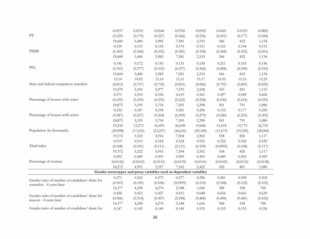
Table 2 presents the statistics for the covariates and the outcome variables used in the empirical

approach. For each variable, we provide an average, standard deviation (in parenthesis) and the

number of observations for that variable. If we consider all of the municipalities, we obtain

approximately 19,000 observations, aggregating all of the mayors’ schooling profiles. However,

when we filter the sample of only elections, in which the candidates for mayor receiving the most

and second most votes were a man and a woman, this number decreases to approximately 2,500

observations (mixed-gender races).

Approximately 32.8% of mixed-gender races had an elected mayor who had completed high

school but had not gone on to higher education, whereas 45% had completed higher education.

14

Insert Table 2 here

Validity of the research design 16

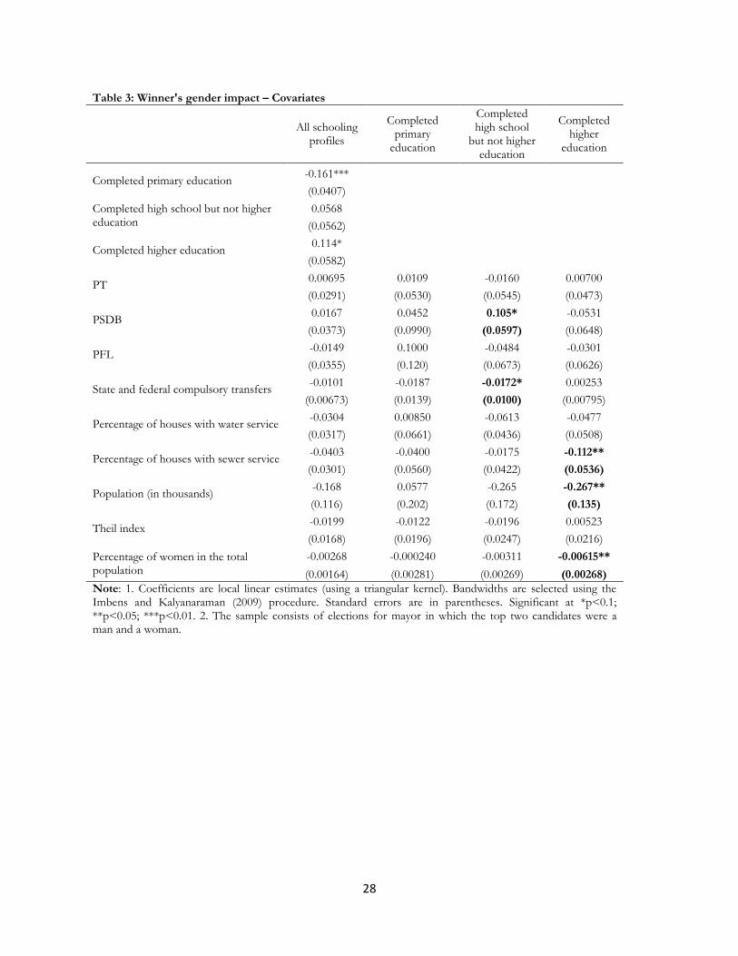
We present three tests of the validity of the research design. First, Table 3 (completed to Figure 1)

shows the schooling of the mayoral candidates, the parties and municipal characteristics (finance,

infrastructure, voters) that could influence the election of women by the margin of victory.

Insert Table 3 here

Insert Figure 1 here

Second, Figure 2 plots the density histogram of mayoral elections by the women’s margin of victory.


Third, Table 4 shows the lagged outcomes as predictors of the women’s margin of victory (Ferreira

and Gyourko (2009) did not conduct the last procedure in their investigation).

Insert Table 4 here

The column “All schooling profiles” in Table 3 shows the difference between women and

men with regard to their levels of schooling; individuals either completed or did not complete their

elementary education and higher education. In both cases, women have higher levels of schooling

than men. There are fewer female mayors who have only completed elementary education (negative

signal) and more female mayors who have finished a higher education course (positive signal). Thus,

the schooling of mayors can have an influence on the election of women in terms of the margin of

victory (note that the discontinuity in the top left panel of Figure 1 confirms only that more female

mayors have completed elementary education – “Completed primary education but not high

school”). The graph in Figure 1 shows the margin of victory when a woman wins on the right-hand

side and when a woman loses (a man wins) on the left-hand side. Each dot corresponds to the

average result inside the bin given the margin of victory obtained by a female mayor. The solid line

16 See Eggers, Folke, Fowler, Hainmueller, Hall and Snyder (2013).

15

in the figures represents the predictive values from a local linear estimation, with 95% confidence

intervals. Thus, fewer winning women (right side) have completed elementary education when

compared with winning men (left side) in the top left of Figure 1.

Considering this result, we developed our main results with three experiments for the

different levels of schooling of mayors. In the same Table 3, the last three columns show these

results (Brollo and Troiano (2012) did not consider this question in their investigation into the

influence of female mayors on federal transfers). Although the PSDB, state and federal compulsory

transfers, percentage of houses with sewer service, population and percentage of women in the total

population show significant discontinuity in the different experiments, they are not confirmed

graphically. No other variable shows a sign of discontinuity around the threshold. We prepared two

supplementary pieces of material for this article, with an additional investigation that sustains our

argument. Supplementary Material 1 includes all of the covariate graphs and the lagged and main

dependent variables of the tables and can be provided upon request by the authors.

Figure 2 shows that there is no indication of discontinuity or endogenous sorting around the

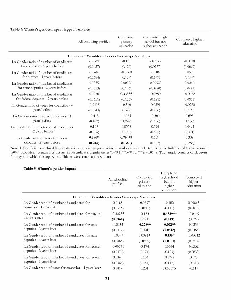
margin of victory threshold. Finally, Table 4 indicates several lagged variables in the different

experiments that are predictors of women’s margin of victory. First, we consider “All schooling

profiles” for the gender ratio of the vote for federal deputies two years before. In the first

experiment (mayors who have completed their elementary education), we indicate the gender ratio

of the number of candidates for federal deputy two years before and the gender ratio of the vote for

federal deputy two years before. We find no significance in any variable in the second and third

experiments. The significant results are not considered in the main discussion given that they may be

predictors of the women’s margin of victory.

16

Main Results

Table 5 depicts the main results. Given the validity of the research design (lagged variables), the

results of the analyses are shown in bold.

Insert Table 5 here

In line with the relevant literature indicating that after being exposed to a female mayor,

voters change their gender stereotype and become more inclined to vote for women in the next

elections, as Beaman, Chattopadhyay, Duflo and Topalova (2009) and Bhavnani (2009) showed for

India, we investigated what happens to both the gender ratio of the number of candidates and the

vote for councilors and mayors (both four years later). For state and federal deputies (two and six

years later – the sequence of elections for other public positions), at each municipality, we computed

both the gender ratio of the number of candidates who received at least one vote and the number of

votes. Considering that the difference in schooling among mayors can affect the discontinuity (the

case in which the mayors have completed their elementary education), our most important results

arose from the schooling group in which mayors had completed high school but not higher

education. These results suggest a significant reduction in the gender ratio of the number of

candidates (fewer women candidates) for mayor (four years later) and the number of candidates with

at least one vote for state deputy (two and six years later) and a reduction in the number of votes for

(women candidate) mayor (four years later).

Without additional robustness tests, we conclude this subsection by observing that there is

evidence that local female politicians are not able to change any gender stereotyping that voters may

have about the role of women in politics, as Beaman, Chattopadhyay, Duflo and Topalova (2009)

suggested for India; unlike these researchers, we find that exposure increases negative gender

stereotyping. It is important to note that the negative reinforcement of gender stereotypes does not

extend to certain public positions (councilor and federal deputy). The most negative result is

17

concentrated on the mayor’s career (candidates and votes). There is no mention of this type of result

in the previous literature.

Robustness

We performed additional robustness tests for the results in which mayors completed high school but

not higher education. Our additional tests involved new regressions, including polynomials (the

square of the margin of victory and the square of the margin of victory interactive with a dummy of

elected women), a closed window of competition (in our case, 10% of the margin of victory: -10%

and +10% of the threshold – our main result was with 30%), the covariates described at the

beginning of this paper and the general results (both terms) in the first and second terms.

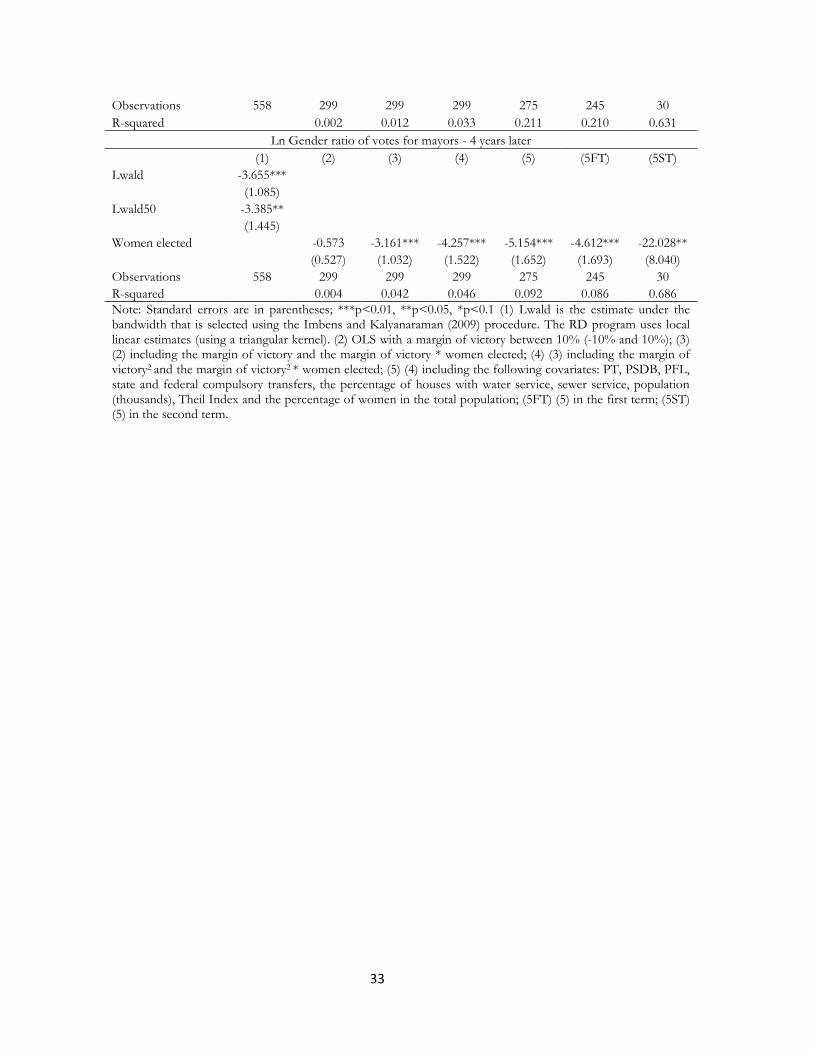
Table 6 provides a different estimate of the variables for which we obtained significance in

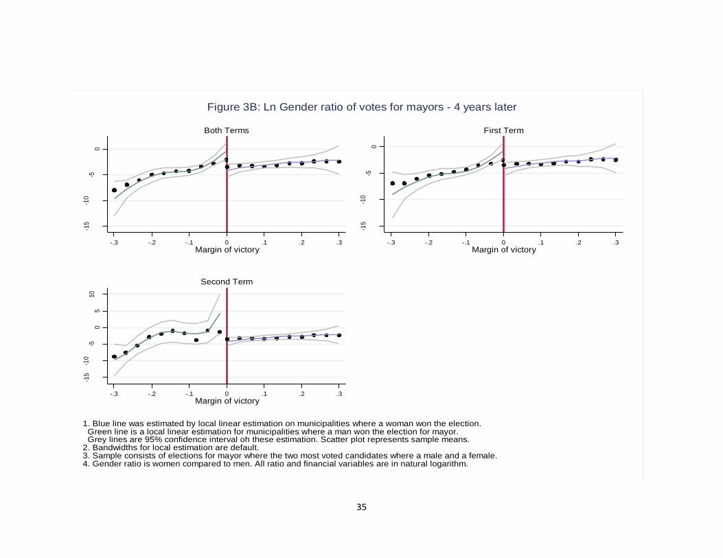
Table 5. Figures 3A and 3B show the results that were fairly significant in Table 6. As previously

noted, all graphs of the variables used in our main investigation are provided in Supplementary

Material 1.

Insert Table 6 here

Insert Figure 3A and 3B here

As shown in Table 6, only the result of the number of candidates and votes for mayors (four

years later) when the mayors have completed their high school education but not higher education is

robust. The result is significant for different specifications (except estimate 2). Figures 3A and 3B

show a discontinuity in both terms independently (first and second terms). When a woman with a

middle-school education is elected in a random process (competitive elections), the number of

women candidates and votes for female mayoral candidates is lower than for male candidates (the

gender ratio is lower). The presence of women in the highest public positions in Brazilian

municipalities has apparently not helped other women to win the office of mayor. Considering that

these results were not significant for other public positions (councilor, state and federal deputies),

18

this finding indicates that the issue is localized. Re-emphasizing the position, this result is different

from Beaman, Chattopadhyay, Duflo and Topalova (2009) and Bhavnani (2009) for India, who

observed an electoral improvement for women when women came into power, and from Ferreira

and Gyourko (2009) with regard to US municipalities, who did not investigate the effect of the

gender of the mayor on future candidates. The main result of Ferreira and Gyourko’s research only

concerns the re-election of women (re-election is easier). Rosenwasser and Dean (1989), Huddy and

Terkildsen (1993) and Lawless (2004) noted that gender stereotyping occurs more frequently at the

federal level than at the local level. We obtained negative results at the local level, even when

considering the few women elected.

Considering the estimate in Column 5, the number of female candidates compared to male

candidates decreases by 68.3%, and the reduction of votes for female candidates compared to male

candidates is even more significant, at 41.5%. There are two men and 0.618 women, on average, in

the sample. In addition, there are 8,332.66 votes for men and 2,846.91 votes for women, on average,

in the sample.

Are there policies that influence gender results?

The evaluations of female candidates and officeholders also generally conform to stereotypical

thinking regarding issue positions. Women are assumed to be more interested in, and more effective

in dealing with, issues such as child care, poverty, education and health care (Dolan, 2010).

Chattopadhyay and Duflo (2001) and Duflo and Topalova (2004), Schwindt-Bayer (2006), Ferreira

and Gyourko (2009) and Brollo and Troiano (2012) investigated whether there are any differences in

gender with regard to policies. Other than Ferreira and Gyourko (2009), all of the studies described

differences in policy between women and men. Using the same methodology as in our primary

investigation, we investigated the effect of a female mayor on specific policies (the number of

municipal daycare centers and vaccines for infants can help women because they facilitate the life of

19

women in the labor market, providing a place for their children to stay and children with less illness)

and on general policies (voluntary transfers from state and federal governments to local government

provide “new” money for carrying out additional policies in the municipality).

Insert Table 7 here

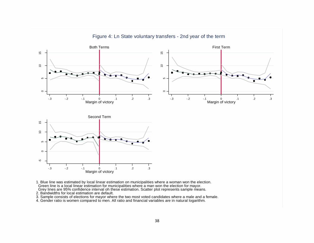
Table 8 corresponds to the last table in our robustness results (Table 6). The definition of

the variables, the descriptive statistics of the variables, lagged and main dependent policy variables

and graphs (difference in the mayor´s schooling and final results for the first and second terms) can

be requested from the authors (Supplementary Material 2). Although there are significant results in

state voluntary transfers – the second year of the term is significant in the estimate (unlike in Brollo

and Troiano (2012)), they are not confirmed graphically (Figure 4). Thus, the gender stereotype

result cannot be linked to policies (specific for women and general policies). This result is the same

as that obtained by Ferreira and Gyourko (2009) for a majoritarian system, although these

researchers did not have the advantage of testing the second term as the term limit, as in the case of

Brazil (avoiding the problems associated with the Downsian process).


Can this result influence the future of young women in politics?

There is a long tradition in the literature showing that women in important public positions can

encourage the political activism of other women. The main idea is that frequent contact with top-

quality "in-group" members predicts stronger implicit self-conceptions of leadership and greater

career ambitions (Asgari, Dasgupta and Cote, 2010). Verba, Burns and Schozman (1997); Hansen

(1997); Atkenson (2003); Campbell and Wolbrecht (2006); and Beaman, Duflo, Pande and Topalova

(2012) are among the researchers who have developed this effect. As we did, Beaman, Duflo, Pande

and Topalova (2012) used a quasi-experiment and found that a positive effect of exposure to a

female leader overrides any possible backlash, probably because this effect gives women a chance to

20

demonstrate that they are capable leaders (there is a role-model effect on girls’ education – a female

politician as a role model leads to more girls seeking to pursue higher education, for instance).

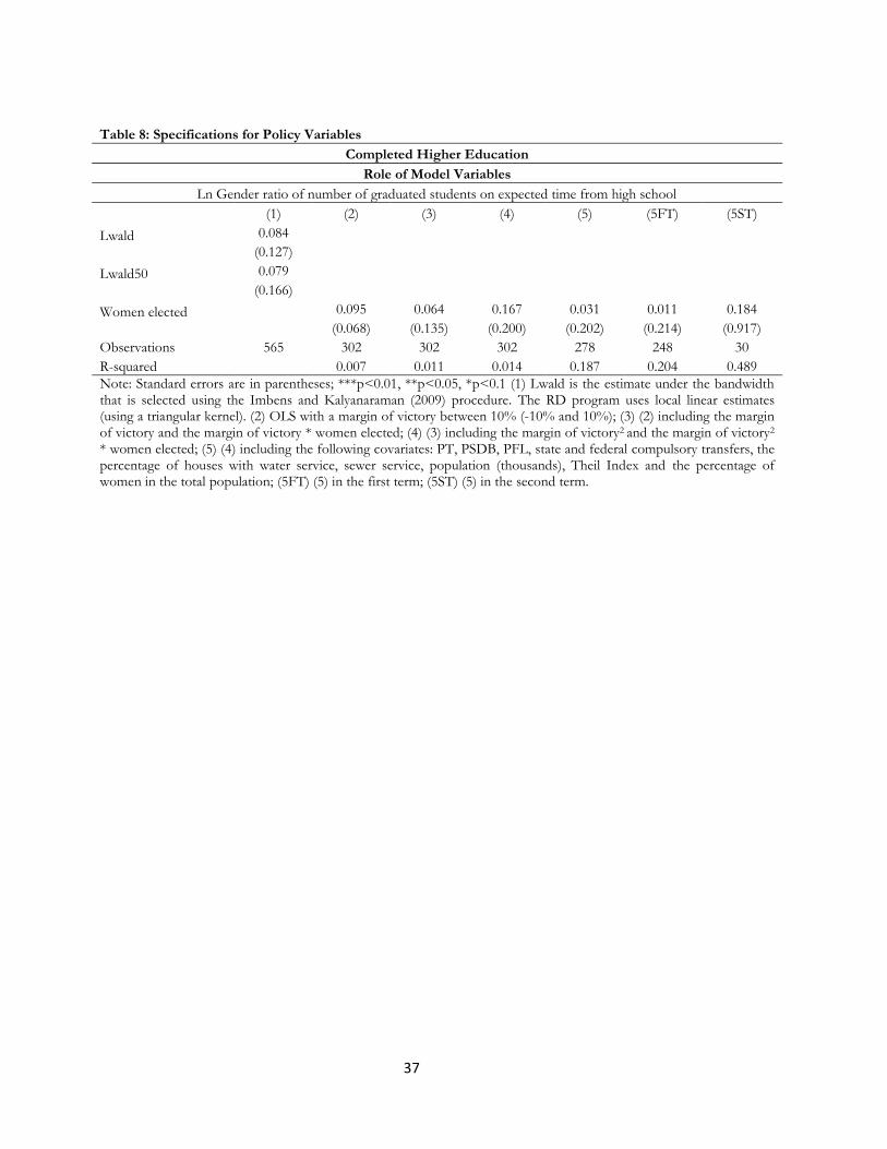
Adopting the same technical procedure as before, we compared the possibility of

adolescents between 16 and 17year-old (the vote is not compulsory for this age) who choose to

participate or not to participate in the election and the schooling of these teenagers. Our results are

depicted in Table 8.

Insert Table 8 here

Table 8 corresponds to the last tables describing our main result (Tables 6 and 7). The

definition of the variables, the descriptive statistics of the variables, lagged and main dependent

policy variables and graphs (difference in the mayors’ schooling and final results for the first and

second terms) can be requested from the authors (Supplementary Material 2). No result was

significant, as was expected considering the previous results. Previous studies did not obtain this

result.

6. Conclusions

Brazilian municipal governments (approximately 5,500 municipalities), their political systems and a

broad range of information enable us to evaluate how the election of a woman to the most

important local position (mayor) affects gender stereotyping. Considering that there is an observed

difference in the schooling of mayors (women are more educated than men), we conducted three

different conditional experiments in our main investigation. We divided the sample into three main

educational groups: mayors who had completed elementary education, mayors who had completed

high school but not higher education and those who had completed higher education. We used

Brazilian electoral data and restricted our focus to close mayoral races (using an RDD design) in

which the top two candidates were of opposite sexes (Lee, 2001; Lee and Card, 2008; Lee, Moretti

and Buttler, 2004).

21

In our most significant result, we documented that the election of a woman to the executive

branch of local government changes the number of candidates and votes for female candidates in

the next election when mayors have completed high school but not higher education, regardless of

the term considered (first or second). Although this result is contrary to the result reported in

previous studies (Beaman, Chattopadhyay, Duflo and Topalova (2009) and Bhavnani (2009)

highlighted an electoral improvement for women when they came into power in India, and Ferreira

and Gyourko (2009) found that women are more easily re-elected in US municipalities), the presence

of women in local executive positions does not harm the local electoral outcomes of women

running for other public positions (councilor, state and federal deputy). In summary, voters do not

electorally reward women who run for a local executive branch after a woman (the same or another)

had previously occupied that position.

We checked the channels for that negative result. We first verified whether there is a gender

difference in policies given that the evaluations of women officeholders also generally conform to

stereotypical thinking regarding position issues. We then investigated whether the result of women

occupying a local leadership position (mayor) can affect the participation of girls in politics (as a

role-model effect).

The specific (policies directed at women) and general results (voluntary transfers negotiated

with state and federal government of additional money to carry out policies in the municipality) of

policies did not affect the main gender stereotype result. This result is the same as that obtained by

Ferreira and Gyourko (2009) for a majoritarian system, although these researchers did not have the

advantage of testing the second term as the term limit, as is the case in Brazil (avoiding the problems

associated with the Downsian process). Brollo and Troiano (2012) suggest that women are more

efficient in bringing in voluntary transfers from the federal government to municipalities, although

their study did not consider the difference in the schooling of mayors.

22

Although the previous literature shows a positive result of leadership as a role model (Verba,

Burns and Schozman, 1997; Hansen, 1997; Atkenson, 2003; Campbell and Wolbrecht, 2006;

Beaman, Duflo, Pande and Topalova, 2012), considering our previous result (for mayors and non-

significant policies), the result of our investigation on role models showed a null effect. Female

mayors do not affect the participation of future generations in politics (girls aged 16-17 years old

choosing to vote and the schooling of girls relative to boys).

Our main conclusion is that although women have recently obtained an important place in

politics, particularly at higher and central levels, there are still important barriers to be surmounted at

local levels. Certainly, replicating outdated policy formulas is not the most effective way to achieve

this goal because the electorate and civil society have been reacting negatively to female politicians

who offer politics as usual.

23

Tables and Figures Table 1.A: Definition of variables, as they were constructed, and their sources

Table 1.B: Definition of variables, as they were constructed, and their sources

17 Currently Democratics (DEM).

Variables Construction of variables Source

Margin of victory The difference in the percentage of votes between female and

male candidates for mayor considering the first and second highest vote getters in the first round of elections.

Superior Electoral Court (TSE) for the election of

1996, 2000, 2004 and 2008 (mayors and

councilors) and 1998, 2002, 2006 and 2010

(state and federal deputies). The TSE has

made electronic data available from Brazilian

elections since 1996. (www.tse.gov.br)

Ln Gender ratio of political variables

The number of candidates and votes for councilors, mayors, state and federal

deputies

Ratio between the logarithm of females and males in the specific variable. Given that the district for state and federal elections is

the state, our municipal variable from these elections considers the geographic locations (municipalities) from which the state and

federal deputies received their votes. To avoid reducing variables when the variable is zero, we changed the level of the variable by

adding one unit before the logarithm transformation:

Ln[(𝑥 + 1)/(𝑦 + 1)].

Schooling of mayors

Completed elementary education; completed high school but not higher

education (dropped out of higher education); and completed higher

education

Dummy variables with values equal to 1 when the definition is met and zero otherwise.

Mayor´s term Elected in either the first or second term Dummy variables with values equal to 1 when the definition is met

and zero otherwise.

Workers Party (PT), Brazilian Social Democracy Party (PSDB) and Liberal

Front Party (PFL)17

Dummy variables with values equal to 1 when the definition is met and zero

otherwise. We included two parties with left-wing ideology (PSDB and PT) and

one party with right-wing ideology(PFL), using as the source the classification of

Latin American Parties, as established by Coopedge (1997)

Workers Party (PT), Brazilian Social Democracy Party (PSDB) and Liberal Front Party (PFL).

http://www.tse.gov.br/

24

Variables Construction of variables Variables Source

State and federal transfers

We use as covariate variable the compulsory transfers (the rule of

transfers is established by laws) received from municipalities. The voluntary

transfers (depending of political negotiations between different levels of government) was used as capacity or not

of mayor takes non- established resources for the municipality for doing

additional public policy: average of mandate and on the second year of

mandate (considering that municipal election is midterm of governor and president elections). It could there be

political support between levels of government. (see Brollo and Troiano,

2012)

We use as covariate variable the compulsory transfers (the rule of

transfers is established by laws) received from municipalities. The voluntary

transfers (depending of political negotiations between different levels of government) was used as capacity or not

of mayor takes non- established resources for the municipality for doing

additional public policy: average of mandate and on the second year of

mandate (considering that municipal election is midterm of governor and president elections). It could there be

political support between levels of government. (see Brollo and Troiano,

2012)

The Brazilian Treasury (www.tesouro.fazenda.gov.br)

Water service Percentage of houses with water in the

municipality

Brazilian Institute of Geography and Statistics (IBGE) – 2000 Census

Sewer service Percentage of houses with sewer service

in the municipality

Population In thousands

Theil Theil index for each municipality

Female population Percentage of women in the total

municipal population

Free immunizations

Number of free immunizations under 1 year old (by 100,000 inhabitants) can

benefit women on labor market because they reduced the probability of diseases

of their children and can work with more facility

(Department of Information of the Unified Health System – Sistema Único de Saúde)

(www.datasus.gov.br

Municipal daycare service on total

Share of municipal daycare service on total municipal daycare service. This

variable was used also because can help women on labor market

National Institute for Research in Education (INEP) under the Ministry of Education.

(www.inep.gov.br) Municipal daycare service

on total public

Share of municipal daycare service on total public daycare service. This

variable was used also because can help women on labor market

http://www.tesouro.fazenda.gov.br/

http://www.datasus.gov.br/

http://www.inep.gov.br/

25

Table 2: Descriptive statistics

All municipalities Mixed-gender races

All schooling profiles

Completed primary

education

Completed high school

but not higher

education

Completed higher

education


Completed primary

education


but not higher

education

Completed higher

education

Covariates

Completed primary education but not high school

0.276

0.216 (0.447)

(0.411)

19,600

2,533

Completed high school but not higher education 0.305

0.328

(0.461)

(0.470) 19,600

2,533

Completed higher education

0.387

0.448 (0.487)

(0.497)

19,600

2,533

Elected in first term 0.867 0.883 0.866 0.869 0.853 0.853 0.855 0.865

(0.340) (0.321) (0.341) (0.337) (0.354) (0.354) (0.353) (0.342)

19,600 5,400 5,985 7,581 2,533 546 832 1,134

Ln Gender ratio of educational variables

The number of graduated students on expected time from municipal primary education, the number of graduated students on expected time from municipal high school, the number of graduated students on expected time from municipal education, the number of graduated students on expected time from primary education, the number of graduated students on expected time from high school, and the number of graduated students on expected time

Ratio between the logarithm of female and male on the specific variable. In order to avoid reducing of variables

when the variable is zero, we changed the level of variable summing one unit

before of logarithm transformation: Ln

National Institute for Research in Education (INEP) under the Ministry of Education.

(www.inep.gov.br)

http://www.inep.gov.br/

26

PT

0.0557 0.0331 0.0546 0.0769 0.0592 0.0421 0.0325 0.0882

(0.229) (0.179) (0.227) (0.266) (0.236) (0.201) (0.177) (0.284)

19,600 5,400 5,985 7,581 2,533 546 832 1,134

PSDB

0.159 0.153 0.145 0.176 0.151 0.161 0.144 0.153

(0.365) (0.360) (0.352) (0.381) (0.358) (0.368) (0.352) (0.361)

19,600 5,400 5,985 7,581 2,533 546 832 1,134

PFL 0.146 0.172 0.145 0.131 0.158 0.211 0.143 0.146

(0.353) (0.377) (0.352) (0.337) (0.364) (0.408) (0.350) (0.353)

19,600 5,400 5,985 7,581 2,533 546 832 1,134

State and federal compulsory transfers

15.14 14.92 15.14 15.31 15.17 14.95 15.15 15.29

(0.813) (0.757) (0.792) (0.821) (0.826) (0.791) (0.801) (0.835)

19,570 5,394 5,977 7,570 2,528 543 831 1,133

Percentage of houses with water

0.571 0.510 0.556 0.619 0.565 0.497 0.549 0.606

(0.235) (0.239) (0.233) (0.222) (0.228) (0.230) (0.218) (0.225)

18,875 5,195 5,754 7,303 2,398 501 791 1,086

Percentage of houses with sewer

0.230 0.187 0.194 0.281 0.206 0.152 0.177 0.250

(0.287) (0.257) (0.264) (0.309) (0.279) (0.240) (0.255) (0.303)

18,875 5,195 5,754 7,303 2,398 501 791 1,086

Population (in thousands)

19,232 12,273 16,493 26,058 19,846 11,618 15,775 26,753

(29,098) (17,633) (23,237) (36,610) (29,100) (11,675) (19,329) (38,000)

19,372 5,322 5,916 7,504 2,502 538 826 1,117

Theil index

0.519 0.515 0.518 0.524 0.525 0.522 0.520 0.530

(0.108) (0.101) (0.111) (0.111) (0.109) (0.0905) (0.108) (0.117)

19,372 5,322 5,916 7,504 2,502 538 826 1,117

Percentage of women

0.492 0.489 0.491 0.495 0.493 0.489 0.492 0.495

(0.0142) (0.0143) (0.0141) (0.0135) (0.0141) (0.0145) (0.0135) (0.0138)

18,272 4,991 5,557 7,102 2,422 520 801 1,080

Gender stereotypes and proxy variables used as dependent variables

Gender ratio of number of candidates’ share for councilor - 4 years later

0.271 0.262 0.275 0.277 0.296 0.281 0.298 0.302

(0.103) (0.105) (0.106) (0.0999) (0.110) (0.108) (0.122) (0.102)

14,377 4,258 4,274 5,348 1,656 388 558 700

Gender ratio of number of candidates’ share for mayors - 4 years later

0.420 0.423 0.427 0.413 0.648 0.656 0.663 0.630

(0.306) (0.314) (0.307) (0.298) (0.468) (0.496) (0.481) (0.432)

14,377 4,258 4,274 5,348 1,656 388 558 700

Gender ratio of number of candidates’ share for 0.147 0.145 0.149 0.149 0.155 0.155 0.153 0.156

27

state deputies - 2 years later (0.0706) (0.0789) (0.0662) (0.0667) (0.0647) (0.0763) (0.0492) (0.0688)

19,332 5,321 5,908 7,488 2,519 543 825 1,130

Gender ratio of number of candidates’ share for state deputies - 6 years later

0.153 0.150 0.155 0.155 0.161 0.158 0.162 0.161

(0.0500) (0.0522) (0.0511) (0.0479) (0.0522) (0.0543) (0.0517) (0.0513)

14,377 4,258 4,274 5,348 1,656 388 558 700

Gender ratio of number of candidates’ share for federal deputies - 2 years later

0.134 0.135 0.136 0.134 0.144 0.145 0.140 0.145

(0.0866) (0.0985) (0.0846) (0.0792) (0.0810) (0.0861) (0.0747) (0.0828)

19,332 5,321 5,908 7,488 2,519 543 825 1,130

Gender ratio of number of candidates’ share for federal deputies - 6 years later

0.137 0.136 0.141 0.138 0.146 0.141 0.145 0.149

(0.0690) (0.0704) (0.0707) (0.0668) (0.0728) (0.0712) (0.0730) (0.0740)

14,377 4,258 4,274 5,348 1,656 388 558 700

Gender ratio of vote share for councilor - 4 years later

0.184 0.182 0.187 0.184 0.209 0.202 0.219 0.206

(0.108) (0.112) (0.111) (0.104) (0.123) (0.126) (0.133) (0.112)

14,377 4,258 4,274 5,348 1,656 388 558 700

Gender ratio of vote share for mayoral candidates - 4 years later

34.80 31.00 41.14 32.78 136.0 128.0 159.5 110.5

(527.1) (411.0) (648.6) (507.5) (1,078) (820.2) (1,341) (910.0)

14,377 4,258 4,274 5,348 1,656 388 558 700

Gender ratio of vote share for state deputies - 2 years later

0.149 0.151 0.152 0.148 0.172 0.169 0.169 0.175

(0.515) (0.524) (0.684) (0.344) (0.455) (0.566) (0.494) (0.359)

19,332 5,321 5,908 7,488 2,519 543 825 1,130

Gender ratio of vote share for state deputies - 6 years later

0.157 0.169 0.148 0.157 0.176 0.151 0.186 0.185

(0.548) (0.840) (0.336) (0.380) (0.410) (0.312) (0.495) (0.385)

14,377 4,258 4,274 5,348 1,656 388 558 700

Gender ratio of vote share for federal deputies - 2 years later

0.0898 0.0937 0.0943 0.0855 0.0871 0.0876 0.0972 0.0793

(0.243) (0.259) (0.257) (0.222) (0.192) (0.203) (0.206) (0.174)

19,332 5,321 5,908 7,488 2,519 543 825 1,130

Gender ratio of vote share for federal deputies - 6 years later

0.0874 0.0879 0.0912 0.0870 0.101 0.108 0.104 0.0949

(0.218) (0.216) (0.216) (0.227) (0.243) (0.296) (0.216) (0.232)

14,377 4,258 4,274 5,348 1,656 388 558 700

Note: The information provided first is the average. Standard errors in parentheses are provided second. The last information provided is the number of observations.

28

Table 3: Winner's gender impact – Covariates


Completed primary

education


but not higher education

Completed higher

education

Completed primary education -0.161***

(0.0407) Completed high school but not higher

education 0.0568

(0.0562)

Completed higher education 0.114*

(0.0582)

PT 0.00695 0.0109 -0.0160 0.00700

(0.0291) (0.0530) (0.0545) (0.0473)

PSDB 0.0167 0.0452 0.105* -0.0531

(0.0373) (0.0990) (0.0597) (0.0648)

PFL -0.0149 0.1000 -0.0484 -0.0301

(0.0355) (0.120) (0.0673) (0.0626)

State and federal compulsory transfers -0.0101 -0.0187 -0.0172* 0.00253

(0.00673) (0.0139) (0.0100) (0.00795)

Percentage of houses with water service -0.0304 0.00850 -0.0613 -0.0477

(0.0317) (0.0661) (0.0436) (0.0508)

Percentage of houses with sewer service -0.0403 -0.0400 -0.0175 -0.112**

(0.0301) (0.0560) (0.0422) (0.0536)

Population (in thousands) -0.168 0.0577 -0.265 -0.267**

(0.116) (0.202) (0.172) (0.135)

Theil index -0.0199 -0.0122 -0.0196 0.00523

(0.0168) (0.0196) (0.0247) (0.0216)

Percentage of women in the total population

-0.00268 -0.000240 -0.00311 -0.00615**

(0.00164) (0.00281) (0.00269) (0.00268)

Note: 1. Coefficients are local linear estimates (using a triangular kernel). Bandwidths are selected using the Imbens and Kalyanaraman (2009) procedure. Standard errors are in parentheses. Significant at *p<0.1; **p<0.05; ***p<0.01. 2. The sample consists of elections for mayor in which the top two candidates were a man and a woman.

29

-.1

0.1

.2.3

.4

-.3 -.2 -.1 0 .1 .2 .3

Margin of victory

Completed primary education but not high school

.1.2

.3.4

.5.6

-.3 -.2 -.1 0 .1 .2 .3

Margin of victory

Completed high school but not higher education

.2.4

.6.8

-.3 -.2 -.1 0 .1 .2 .3

Margin of victory


1. Blue line was estimated by local linear estimation on municipalities where a woman won the election. Green line is a local linear estimation for municipalities where a man won the election for mayor. Grey lines are 95% confidence interval oh these estimation. Scatter plot represents sample means.2. Bandwidths for local estimation are default.3. Sample consists of elections for mayor where the two most voted candidates where a male and a female.4. Gender ratio is women compared to men. All ratio and financial variables are in natural logarithm.

Figure 1: Mayor's schooling profiles

30

050

10

015

0

ab

solu

te fre

qu

en

cy

-.3 -.2 -.1 0 .1 .2 .3Margin of victory

2 p.p. 1 p.p.

0.5 p.p.

Figure 2: Frequency of margin of victory - mixed-gender races

31

Table 5: Winner's gender impact


Completed primary

education


but not higher

education

Completed higher

education

Dependent Variables - Gender Stereotype Variables

Ln Gender ratio of number of candidates for councilor - 4 years later

0.0188 -0.0667 -0.182 0.00865

(0.0516) (0.0915) (0.111) (0.0818)

Ln Gender ratio of number of candidates for mayors - 4 years later

-0.232** -0.153 -0.485*** -0.0169

(0.0960) (0.171) (0.149) (0.122)

Ln Gender ratio of number of candidates for state deputies - 2 years later

-0.0653 -0.278** -0.102** 0.0336

(0.0412) (0.121) (0.0512) (0.0464)


-0.0599 0.00813 -0.135* -0.00342

(0.0485) (0.0999) (0.0701) (0.0574)

Ln Gender ratio of number of candidates for federal deputies - 2 years later

-0.00671 -0.174 0.0544 0.0562

(0.0471) (0.174) (0.103) (0.0833)

Ln Gender ratio of number of candidates for federal deputies - 6 years later

0.0364 0.134 -0.0748 0.173

(0.0583) (0.134) (0.117) (0.121)

Ln Gender ratio of votes for councilor - 4 years later 0.0814 0.201 0.000576 -0.117

Table 4: Winner's gender impact-lagged variables

All schooling profiles Completed

primary education

Completed high school but not

higher education



Ln Gender ratio of number of candidates for councilor - 4 years before

-0.0591 -0.111 -0.0533 -0.0878

(0.0427) (0.120) (0.0777) (0.0669)

Ln Gender ratio of number of candidates for mayors - 4 years before

-0.0685 -0.0660 -0.106 0.0596

(0.0684) (0.164) (0.149) (0.144)

Ln Gender ratio of number of candidates for state deputies - 2 years before

0.0235 0.00386 -0.00529 0.0246

(0.0353) (0.106) (0.0770) (0.0481)

Ln Gender ratio of number of candidates for federal deputies - 2 years before

0.0276 0.339** -0.0559 -0.0422

(0.0651) (0.133) (0.121) (0.0951)

Ln Gender ratio of votes for councilor - 4 years before

-0.0438 -0.310 -0.0391 -0.0270

(0.0843) (0.397) (0.156) (0.123)

Ln Gender ratio of votes for mayors - 4 years before

-0.415 -1.075 -0.303 0.695

(0.477) (1.247) (1.136) (1.135)

Ln Gender ratio of votes for state deputies - 2 years before

0.109 0.0558 0.324 0.0462

(0.206) (0.449) (0.422) (0.371)

Ln Gender ratio of votes for federal deputies - 2 years before

0.396* 0.754** 0.129 0.308

(0.214) (0.380) (0.395) (0.288)

Note: 1. Coefficients are local linear estimates (using a triangular kernel). Bandwidths are selected using the Imbens and Kalyanaraman (2009) procedure. Standard errors are in parentheses. Significant at *p<0.1; **p<0.05; ***p<0.01. 2. The sample consists of elections for mayor in which the top two candidates were a man and a woman.

32

(0.104) (0.222) (0.155) (0.169)

Ln Gender ratio of votes for mayors - 4 years later -1.524** -1.297 -3.655*** 0.00682

(0.743) (1.271) (1.085) (1.079)

Ln Gender ratio of votes for state deputies - 2 years later

-0.0521 0.0698 -0.272 -0.0875

(0.139) (0.343) (0.324) (0.224)

Ln Gender ratio of votes for state deputies - 6 years later

0.217 0.430 0.115 0.185

(0.211) (0.502) (0.292) (0.441)

Ln Gender ratio of votes for federal deputies - 2 years later

0.0320 -0.497 0.120 0.140

(0.187) (0.500) (0.369) (0.274)

Ln Gender ratio of votes for federal deputies - 6 years later

0.249 0.187 0.110 0.428

(0.229) (0.435) (0.411) (0.403)

Note: 1. Coefficients are local linear estimates (using a triangular kernel). Bandwidths are selected using the Imbens and Kalyanaraman (2009) procedure. Standard errors are in parentheses. Significant at *p<0.1; **p<0.05; ***p<0.01. 2. The sample consists of elections for mayor in which the top two candidates were a man and a woman. The gender ratio is women compared to men.

Table 6: Robustness - additional specifications



Ln Gender ratio of number of candidates for mayors - 4 years later

(1) (2) (3) (4) (5) (5FT) (5ST)

Lwald -0.485***

(0.149)

Lwald50 -0.405**

(0.204)

Women elected

-0.052 -0.409*** -0.584*** -0.683*** -0.579** -2.724***

(0.071) (0.139) (0.205) (0.222) (0.232) (0.918)

Observations 558 299 299 299 275 245 30

R-squared 0.002 0.046 0.051 0.109 0.097 0.730


(1) (2) (3) (4) (5) (5FT) (5ST)

Lwald -0.102**

(0.051)

Lwald50 -0.080

(0.066)

Women elected

-0.101*** -0.071 -0.104 -0.066 -0.078 0.005

(0.034) (0.068) (0.098) (0.099) (0.109) (0.230)

Observations 825 433 433 433 393 341 52

R-squared 0.020 0.021 0.022 0.206 0.208 0.468


(1) (2) (3) (4) (5) (5FT) (5ST)

Lwald -0.135*

(0.070)

Lwald50 -0.166*

(0.093)

Women elected

-0.026 -0.143* -0.184* -0.073 -0.068 -0.470

(0.038) (0.076) (0.111) (0.111) (0.115) (0.555)

33

Observations 558 299 299 299 275 245 30

R-squared 0.002 0.012 0.033 0.211 0.210 0.631

Ln Gender ratio of votes for mayors - 4 years later

(1) (2) (3) (4) (5) (5FT) (5ST)

Lwald -3.655***

(1.085)

Lwald50 -3.385**

(1.445)

Women elected

-0.573 -3.161*** -4.257*** -5.154*** -4.612*** -22.028**

(0.527) (1.032) (1.522) (1.652) (1.693) (8.040)

Observations 558 299 299 299 275 245 30

R-squared 0.004 0.042 0.046 0.092 0.086 0.686

Note: Standard errors are in parentheses; ***p<0.01, **p<0.05, *p<0.1 (1) Lwald is the estimate under the bandwidth that is selected using the Imbens and Kalyanaraman (2009) procedure. The RD program uses local linear estimates (using a triangular kernel). (2) OLS with a margin of victory between 10% (-10% and 10%); (3) (2) including the margin of victory and the margin of victory * women elected; (4) (3) including the margin of victory2 and the margin of victory2 * women elected; (5) (4) including the following covariates: PT, PSDB, PFL, state and federal compulsory transfers, the percentage of houses with water service, sewer service, population (thousands), Theil Index and the percentage of women in the total population; (5FT) (5) in the first term; (5ST) (5) in the second term.

34

-2-1

.5-1

-.5

0

-.3 -.2 -.1 0 .1 .2 .3

Margin of victory

Both Terms

-2-1

.5-1

-.5

0

-.3 -.2 -.1 0 .1 .2 .3

Margin of victory

First Term-2

-10

1

-.3 -.2 -.1 0 .1 .2 .3

Margin of victory

Second Term


Figure 3A: Ln Gender ratio of number of candidates for mayors - 4 years later

35

-15

-10

-50

-.3 -.2 -.1 0 .1 .2 .3

Margin of victory

Both Terms

-15

-10

-50

-.3 -.2 -.1 0 .1 .2 .3

Margin of victory

First Term

-15

-10

-50

510

-.3 -.2 -.1 0 .1 .2 .3

Margin of victory

Second Term


Figure 3B: Ln Gender ratio of votes for mayors - 4 years later

36

Table 7: Specifications for Policy Variables


Ln State voluntary transfers - 2nd year of the term

(1) (2) (3) (4) (5) (5FT) (5ST)

Lwald 2.533*

(1.313)

Lwald50 3.669**

(1.743)

Women elected

-0.410 0.984 3.971** 3.876** 1.948 17.672***

(0.604) (1.195) (1.729) (1.828) (2.000) (4.889)

Observations 657 328 328 328 299 250 49

R-squared 0.001 0.015 0.034 0.146 0.159 0.425

Number of per capita free immunizations under 1 year old

(1) (2) (3) (4) (5) (5FT) (5ST)

Lwald 0.045*

(0.024)

Lwald50 0.056*

(0.033)

Women elected

0.019* 0.016 0.052* 0.008 0.004 0.058

(0.010) (0.021) (0.030) (0.024) (0.026) (0.116)

Observations 565 302 302 302 278 248 30

R-squared 0.011 0.012 0.023 0.493 0.504 0.586

Completed Higher Education

Share of municipal on total daycare service

(1) (2) (3) (4) (5) (5FT) (5ST)

Lwald

-0.036

(0.085)

Lwald50

-0.060

(0.113)

Women elected

0.020 -0.037 -0.122 -0.143 -0.184 0.525

(0.045) (0.090) (0.134) (0.142) (0.155) (0.649)

Observations 441 234 234 234 214 190 24

R-squared 0.001 0.005 0.010 0.178 0.180 0.555

Share of municipal on public daycare service

(1) (2) (3) (4) (5) (5FT) (5ST)

Lwald

0.000

(0.004)

Lwald50

-0.002

(0.002)

Women elected

-0.002 0.008 -0.009 -0.006 -0.005 -0.000

(0.004) (0.007) (0.011) (0.013) (0.014) (0.021)

Observations 395 210 210 210 191 168 23

R-squared 0.001 0.017 0.040 0.106 0.117 0.679

Note: Standard errors are in parentheses; ***p<0.01, **p<0.05, *p<0.1 (1) Lwald is the estimate under the bandwidth that is selected using the Imbens and Kalyanaraman (2009) procedure. The RD program uses local linear estimates (using a triangular kernel). (2) OLS with a margin of victory between 10% (-10% and 10%); (3) (2) including the margin of victory and the margin of victory * women elected; (4) (3) including the margin of victory2 and the margin of victory2 * women elected; (5) (4) including the following covariates: PT, PSDB, PFL, state and federal compulsory transfers, the percentage of houses with water service, sewer service, population (thousands), Theil Index and the percentage of women in the total population; (5FT) (5) in the first term; (5ST) (5) in the second term.

37

Table 8: Specifications for Policy Variables

Completed Higher Education

Role of Model Variables

Ln Gender ratio of number of graduated students on expected time from high school

(1) (2) (3) (4) (5) (5FT) (5ST)

Lwald

0.084

(0.127)

Lwald50

0.079

(0.166)

Women elected

0.095 0.064 0.167 0.031 0.011 0.184

(0.068) (0.135) (0.200) (0.202) (0.214) (0.917)

Observations 565 302 302 302 278 248 30

R-squared 0.007 0.011 0.014 0.187 0.204 0.489

Note: Standard errors are in parentheses; ***p<0.01, **p<0.05, *p<0.1 (1) Lwald is the estimate under the bandwidth that is selected using the Imbens and Kalyanaraman (2009) procedure. The RD program uses local linear estimates (using a triangular kernel). (2) OLS with a margin of victory between 10% (-10% and 10%); (3) (2) including the margin of victory and the margin of victory * women elected; (4) (3) including the margin of victory2 and the margin of victory2

* women elected; (5) (4) including the following covariates: PT, PSDB, PFL, state and federal compulsory transfers, the percentage of houses with water service, sewer service, population (thousands), Theil Index and the percentage of women in the total population; (5FT) (5) in the first term; (5ST) (5) in the second term.

38

05

10

15

-.3 -.2 -.1 0 .1 .2 .3

Margin of victory

Both Terms

05

10

15

-.3 -.2 -.1 0 .1 .2 .3

Margin of victory

First Term

-50

510

15

-.3 -.2 -.1 0 .1 .2 .3

Margin of victory

Second Term


Figure 4: Ln State voluntary transfers - 2nd year of the term

39

References

Arvate, P.R.(2013) Electoral Competition and Local Government Responsiveness in Brazil. World Development, vol 43, pp. 67–83

Asgari, S., Dasgupta, N., and Cote, N.G. (2010) When does contact with successful in-group memberschange self-stereotypes? A longitudinal study comparing the effect of quantity vs. quality ofcontact with successful individuals. Social Psychology, 41, pp. 201- 202

Atkeson, L.R. (2003). Not All Cues Are Created Equal: The Conditional Impact of Female Candidates on Political Engagement. Journal of Politics 65(4): 1040–61.

Beaman, L., Chattopadhyay, R., Duflo, E., Pande, R., and P. Topalova (2012), Female Leadership Raises Aspirations and Educational Attainment for Girls: A Policy Experiment in India, Science 335 (582), DOI: 10.1126/science.1212382

Beaman, L., Chattopadhyay, R., Duflo, E., Pande, R., and P. Topalova (2009), “Powerful Women: Does Exposure Reduce Bias?” Quarterly Journal of Economics 124(4), pp. 1497-1540.

Bhavnani, R.R. (2009) Do Electoral Quotas Work after They Are Withdrawn? Evidence from a Natural Experiment in India. American Journal of Political Science,vol. 103, pp. 23-35.

Brollo, F. and U. Troiano (2012) What Happens When a Woman Wins a Close Election? Evidence from Brazil. Typescript.

Campbell, D. E. and Wolbrecht, C. (2006) Women Politicians as Role Models for Adolescents.The Journal of Politics, Volume 68, Issue 02, pp. 233-247

Cleary, M. R. (2007). Electoral Competition, Participation, and Government Responsiveness in Mexico. American Journal of Political Science, v. 51(2), pp. 283-299

Chattopadhyay, R. and Duflo, E. (2004) Women as Policy Makers: Evidence from a India-Wide Randomized Policy Experiment. Econometrica 72, 5: 1409- 1444

Dolan, K. (2010). The Impact of Gender Stereotyped Evaluations on Support for Women Candidates Political Behavior 32: 69-88

Downs, A. (1957) An Economic Theory of Democracy. Boston, MA: Addison-Wesley. Duflo, E. and Topalova, P.(2005) Unappreciated Service: Performance, Perceptions, and Women

Leaders in India, MIT Mimeo. http://econ-www.mit.edu/files/793 Eggers, A.C. Folke, O. Fowler, A. Hainmuller, J. Hall, A.B. and Snyder, J.M. (2013) On the validity of

Regression Discontinuity Design for estimating electoral effects: new evidence from over 40,000 close races. MIT Political Science Working Paper Series number 26.

Ferreira, F. and Gyourko, J. (2009) Do Political Parties Matter? Evidence from U.S. Cities-super, The Quarterly Journal of Economics, vol. 124(1), pp. 399-422

Hansen, S. (2008) Talking About Politics: Gender and Contextual Effects on Political ProselytizingThe Journal of Politics, Vol. 59, No. 1 (Feb., 1997), pp. 73-103

Hecock, D. R. (2006). Electoral Competition, Globalization, and Subnational Education Spending in Mexico, 1999–2004, American Journal of Political Science, v. 50 (4), p.950-961.

Huddy, L. and Terkildsen, N. (1993) The Consequences of Gender Stereotypes for Women Candidates at Different Levels and Types of Offices. Political Research Quarterly. 46: 503-525.

Hughes, M.M. (2011) Intersectionality, Quotas, and Minority Women’s Political Representation Worldwide. American Political Science Review, Volume 105, Issue 03, pp. 604-620

Lawless, J. (2004). Women, War, and Winning Elections: Gender Stereotyping in the post-September 11th Era. Political Research Quarterly 57: 479-490.

Lawless, J.L. and Pearson, K. (2008) The Primary Reason for Women's Underrepresentation? Reevaluating the Conventional Wisdom. The Journal of Politics, Vol. 70, No. 1, pp. 67-82

http://econ-www.mit.edu/files/793

40

Lawless, J.L. and Theriault, S.M. (2009) Will she stay or will she go? Legislative Studies Quarterly, Vol. 30, No. 4, pp.581-96.

Lee, D. (2001) The Electoral Advantage to Incumbency and Voters’ Valuation ofPoliticians’ Experience: A Regression Discontinuity Analysis of Elections tothe U.S. House, NBER Working Paper No. 8441.

Lee, D. and Card, D. (2008) Regression Discontinuity Inference with SpecificationError,” Journal of Econometrics, 142 (2008), pp. 655–674.

Lee, D. Moretti, E. and Butler, M. (2004) Do Voters Affect or Elect Policies? Evidence from the U.S. House,Quarterly Journal of Economics, 119(2004), 807–859.

Lindbeck, A. and Weibull, J. W. (1988) Balanced-budget redistribution as the outcome of political competition. Public Choice, vol. 52, p. 273-297.

Mainwaring, S. P. (2002). Rethinking Party Systems in the Third Wave of Democratization: The case of Brazil. Stanford University Press.

Persson, T. and Tabellini, G. (2000). Political Economics: explaining economic policy. The MIT Press. Peltzman, S. (1992). Voters as fiscal conservatives. Quarterly Journal of Economics, v. 100(2), p.327-361. Perotti, R. and Kontopoulos, Y. (2002). Fragmented Fiscal Policy. Journal of Public Economics,86(2),

pp.191-222. Power, T. J. (2009).Compulsory for Whom?Mandatory voting and electoral participation in Brazil,

1986-2006.Journal of Politics in Latin America, v.1(1), p.97-122 Rosenwasser, S. and Dean, N. (1989). Gender Role and Political Office: Effects of Perceived

Masculinity/Femininity of Candidate and Political Office. Psychology of Women Quarterly 13: 77-85.

Samman, E. and Santos, M. E. (2009). Agency and Empowerment: Areview of concepts, indicators, and empirical evidence, FirstDraft. Oxford Poverty and Human Development Initiative, TheUniversity of Oxford

Samuels, D.(1997). Determinantes do Voto Partidário em Sistemas Eleitorais Centrados no Candidato: Evidências sobre o Brasil.Dados, v.40(3)

Shepsle, K., Weingast, B., (1981). Political preferences for the pork barrel: a generalization. American Journal of Political Science 25 (1), pp. 96–111.

Schwindt-Bayer, L.A. (2006). Still Supermadres? Gender and the Policy Priorities of Latin American Legislators American Journal of Political Science,Vol. 50, No. 3, pp. 570–585

Verba, S., Schozman, K. and Brady, H. E. (1995). Voice and equality: Civic voluntarism in American politics. Harvard University Press.

Verba, S., Burns, N., and Schlozman, K.L. (1997) Knowing and Caring about Politics: Gender and Political Engagement. The Journal of Politics, Vol. 59, No. 4 (Nov., 1997), pp. 1051-1072

WORKING PAPER 1/2014 • JAN, 2014 •

Os artigos dos Textos para Discussão da Escola de Economia de São Paulo da Fundação Getulio Vargas são de inteira responsabilidade dos autores e não refletem necessariamente a opinião da FGV-EESP. É permitida a reprodução total ou parcial dos artigos, desde que creditada a fonte.

Escola de Economia de São Paulo da Fundação Getulio Vargas FGV-EESP

www.fgvsp.br/economia

Documents

Working Paper · To achieve our target, we adopted the same strategy used by Ferreira and Gyourko (2009) for US cities, a regression discontinuity design (RDD)