Working Paper Series - European Central Bank · Working Paper Series . Monetary policy and bank profitability in a low interest rate environment . Carlo Altavilla , Miguel Boucinha,

Working Paper Series Monetary policy and bank profitability in a low interest rate environment

Carlo Altavilla, Miguel Boucinha, José-Luis Peydró

Disclaimer: This paper should not be reported as representing the views of the European Central Bank (ECB). The views expressed are those of the authors and do not necessarily reflect those of the ECB.

No 2105 / October 2017

Abstract

We analyse the impact of standard and non-standard monetary policy measures on bank profitability. For empirical identification, the analysis focuses on the euro area, thereby exploiting substantial bank and country heterogeneity within a monetary union where the central bank has implemented a broad range of unconventional policies, including quantitative easing and negative interest rates. We use both proprietary and commercial data on individual bank balance sheets and financial market prices. Our results show that monetary policy easing – a decrease in short-term interest rates and/or a flattening of the yield curve – is not associated with lower bank profits once we control for the endogeneity of the policy measures to expected macroeconomic and financial conditions. Importantly, our analysis indicates that the main components of bank profitability are asymmetrically affected by accommodative monetary conditions, with a positive impact on loan loss provisions and non-interest income largely offsetting the negative one on net interest income. We also find that a protracted period of low interest rates might have a negative effect on profits that, however, only materialises after a long period of time and tends to be counterbalanced by improved macroeconomic conditions. In addition, while more operationally efficient banks benefit more from monetary policy easing, banks engaging more extensively in maturity transformation experience a higher increase in profitability after a steepening of the yield curve. Finally, we assess the impact of unconventional monetary policies on market-based measures of expected bank profitability and credit risk, by employing an event study analysis using high frequency data, and find that accommodative monetary policies tend to increase bank stock returns and reduce credit risk.

JEL: E52, E43, G01, G21, G28.

Keywords: bank profitability, monetary policy, lower bound, quantitative easing, negative rates.

ECB Working Paper 2105, October 2017 1

1

Non-technical summary

Western Europe and the USA suffered a severe banking crisis in late 2000s, followed by a deep economic recession with substantial costs in terms of aggregate output and employment. Central banks reacted strongly to the adverse financial and economic conditions by reducing their policy interest rates and by implementing a broad range of unconventional policies including credit and quantitative easing as well as negative interest rates.

In this paper we analyse the impact of standard and non-standard monetary policy on bank profitability. This topic has important policy implications, as banks’ ability to generate adequate profits is relevant for the sustainability of the banking system and, as such, for its capacity to provide sufficient credit to the economy. Profitable banks are not only able to attract capital from market investors, but can also generate capital internally through retained earnings. Hence, adequate bank profitability contributes towards bank soundness and therefore towards financial stability.

Accommodative monetary policy actions affect bank profitability through different channels with an unclear ex ante net effect. On the one hand, the reduction in interest rates and the associated positive impact on macroeconomic conditions can support banks by reducing funding costs and increasing borrower creditworthiness. On the other hand, monetary accommodation might lead to a contraction in net interest income.

Using data from commercial providers as well as ECB proprietary data over different subsamples we find that changes in the level and the slope of the term structure are not associated with lower bank profits once we control for the endogeneity of the policy measures to (current and expected) macroeconomic and financial conditions. In other words, while periods of low interest rates tend to coincide with lower bank profitability, this is not a causal relationship. Instead, this relationship is confounded by the fact that banks are hampered by weak macroeconomic dynamics and, at the same time, interest rates set by central banks respond to these macroeconomic dynamics.

Importantly, when assessing the impact of monetary policy accommodation on the components of bank profitability we find that the adverse effects on net interest margins are largely offset by the positive impact on intermediation activity and credit quality. Moreover, a further positive (although possibly not long-lasting) effect of unconventional policies on bank profitability is related to the capital gains derived from the increase in the value of the securities held by banks.

The analysis also evaluates whether maintaining interest rates at a low (or even negative) level for an extended period of time might alter the relationship between monetary policy easing and bank profitability. Our results suggest that although keeping interest rates low-for-long might have negative consequences on bank profitability, substantial adverse effects only materialise after a relatively long period of time and tend to be counterbalanced by improvements in macroeconomic conditions associated with low interest rates.

Finally, we assess the impact of non-standard monetary policies on market-based expectations of future profitability, as measured by stock market returns of individual banks. Using a high-frequency event-study approach to isolate the unexpected component of the policy change we find that equity prices increased for the vast majority of banks after all major monetary policy easing announcements made by the European Central Bank, with a significant positive impact also on banks’ credit risk. This is important not only for financial stability and systemic risk but also for the possible distributional consequences that these policies may have on bank shareholders and debtholders, including depositors.


1 Introduction

Western Europe and the United States suffered a severe banking crisis in late 2000s followed by a

deep and long-lasting economic recession, with substantial costs in terms of aggregate output and

employment. A key channel through which the weakness in bank balance sheets affects the real

economy works via the reduction in the supply of bank credit, including deleveraging and asset fire

sales (Bernanke, 1983; Freixas, Laeven and Peydró, 2015). Historically, financial crises triggered

persistent negative effects on the overall economy (Kindelberger, 1978; Reinhart and Rogoff, 2009).

In the recent crisis, for example, the euro area only returned to its pre-crisis GDP levels in 2015, i.e.

eight years after the crisis started. Central banks responded strongly to the banking and economic

crisis, reducing their policy interest rates and implementing several unconventional monetary

policies that have also influenced the slope of the yield curve; some commentators have even

suggested that monetary policy was the only game in town to overcome the economic and financial

problems (El-Erian, 2016).

Lower policy rates and accommodative unconventional monetary policies are in general crucial to

address a weak macroeconomic environment also supporting the financial and banking system.

This is because such measures provide abundant access to central bank liquidity and lower the cost

of debt with positive consequences for bank funding and borrower creditworthiness respectively,

thereby supporting bank capital and reducing non-performing loans and loan loss provisioning

(Bernanke and Gertler, 1995; Praet, 2016; Bernanke, 2007; Diamond and Rajan, 2006; Freixas and

Jorge, 2008; Gertler and Karadi, 2011, 2013; Kiyotaki and Moore, 2012; Freixas, Martin and Skeie,

2011; Allen, Carletti and Gale, 2009 and 2014). At the same time, there may also be some

downsides associated with conventional and unconventional monetary policy easing (Rajan, 2005;

Taylor, 2008; Allen and Rogoff, 2011; Stein, 2012 and 2014; Stiglitz, 2016), including a potential

reduction in net interest income (Borio et al., 2017; Alessandri and Nelson, 2015) which could

ultimately hamper the transmission of monetary policy (Brunnermeier and Koby, 2017). The net

effect of monetary policy on bank profitability therefore remains an empirical question. Moreover,

an important related question is whether a scenario of low (or even negative) rates protracted for an

extended period of time alters the relationship between monetary policy easing and bank

profitability.

These issues have crucial policy implications, as the ability of banks to generate adequate profits is

relevant for the sustainability of the banking system and, as such, for its capacity to provide

sufficient credit to the economy. Profitable banks are not only able to attract capital from market

investors, but they can also generate capital internally through retained earnings. As such, bank

profitability contributes to bank soundness and hence to financial stability (Admatti and Helwig,

2013; Freixas and Rochet, 2008).


In this paper, we analyse the impact of standard and non-standard monetary policy on bank

profitability. For empirical identification, we focus on the euro area, which provides an interesting

laboratory as it features substantial bank and country heterogeneity within a monetary union and the

European Central Bank (ECB) has implemented a broad set of unconventional policies, including

negative interest rates, credit and quantitative easing measures. We use proprietary ECB data on

individual bank balance sheet also combining data from several commercial providers collected

since the creation of the euro area. We study not only the average impact of monetary policy on

bank profits but also its heterogeneous effects depending on banks’ maturity transformation, and

balance sheet characteristics. In addition, as there have been growing concerns over recent years

that the net benefits of accommodative policies might be declining over time (Brunnermeier and

Koby, 2017; Claessens, 2017), we examine whether a protracted period of low interest rates might

impair bank profitability. The analysis also explores the main channels though which monetary

policy actions influence bank profitability. At a micro level, bank-level data are used to analyse the

impact of interest rate changes on the main components of bank profitability – i.e. net interest

income, non-interest income and provisions. We complement this evidence by investigating the

macroeconomic implications of changes in monetary conditions on the same components using a

dynamic multivariate model.

Finally, we assess the impact of non-standard monetary policies on market-based expectations of

future profitability, as measured by stock market returns of individual banks. As the vast majority of

the stakeholders of a bank are debtholders we also investigate the impact of policy measures on

market participants’ perception of banks’ credit risk, as proxied by banks’ CDS spreads, thereby

covering the impact for all the major stakeholders of a bank, ultimately including depositors and

taxpayers. The dynamics of both bank stock prices and CDS are affected by a wide range of factors,

making it particularly challenging to identify the effects of monetary policy due to endogeneity and

simultaneity issues. Moreover, being forward-looking, financial market prices tend to react to

information about policy changes only if these changes are unanticipated. Therefore, to correctly

identify the impact of monetary policy, we use an event-study approach to isolate the unexpected

component of the policy change by looking at the high-frequency movements in asset prices

following monetary policy announcements (see, for example, Bernanke and Kuttner, 2005;

Gürkaynak, Sack and Swanson, 2005b). The identifying assumption is that changes in financial

assets occurring in a small window around a given policy announcement capture the (efficient)

market reaction to the arrival of new information, thereby reflecting the causal impact of the policy.

This paper contributes to the literature on the impact of monetary policy actions on bank

profitability. Early studies document the existence of a positive correlation between interest rates

(usually expressed as level or slope of the term structure) and bank interest margins. This positive

association is interpreted as a natural consequence of banks’ maturity transformation activities (e.g.


Flannery, 1981; Hancock, 1985; Bourke, 1989; Saunders and Schumacher, 2000). Recent studies

have also highlighted the possible trade-off between accommodative monetary policy and bank

profitability. In general, the empirical evidence found in these studies suggests an adverse impact of

monetary policy easing on net interest margins (Alessandri and Nelson, 2015; Borio et al., 2017),

with amplification effects in low interest rate environments (Claessens et al., 2017).

Using a wide range of different data and econometric techniques we establish a set of robust

results.

First, we contribute to the existing literature by finding that when evaluating the impact of

monetary policy on bank profitability it is very important to consider the effects stemming from not

only actual but also expected real economic activity. We are, to our knowledge, the first to use the

expected (forecasted) macroeconomic developments and (forward-looking) credit risk among the

possible set of controls. We find that low monetary policy rates and a reduced slope of the yield

curve are associated with lower bank profits only if there are important variables omitted in the

assessment. More specifically, according to economic theory and central bank practice (see, for

example, Bernanke and Gertler, 1995), monetary policy reacts (is endogenous) to the current and

expected overall economic and financial conditions.1 If we control for overall expected aggregate

economic and financial conditions, the association between monetary policy conditions and bank

profitability breaks down. In other words, controlling for expected (in addition to current)

economic and financial conditions is sufficient to eliminate the correlation between monetary policy

and bank profitability. Bank balance sheet characteristics, such as bank capital, liquidity, non-

performing loans and efficiency, are also important. This is not surprising, as weakness in bank

balance sheets (and the associated impairment in the transmission mechanism) was an important

motivation for monetary policy easing during the crisis (Praet, 2016).

Second, the main components of bank profitability are asymmetrically affected by accommodative

monetary policies with the positive impact on loan loss provisions and non-interest income largely

offsetting the negative one on net interest income, a robust result stemming from both micro and

macro approaches.

Third, we find that heterogeneity of bank balance sheet characteristics matters for the

transmission of monetary policy to bank profitability. Results suggest that an accommodative

monetary policy is relatively more beneficial for banks with higher operational efficiency and banks

with lower asset quality. Additionally, a steepening of the yield curve has a relatively more positive

1 There is a large literature on the monetary policy transmission mechanism that explores the impact of monetary policy, and in general central bank policies, on the economy, via banks (Bernanke and Blinder, 1988 and 1992; Kaskyap and Stein, 2000; Diamond and Rajan, 2006; Gertler and Kiyotaki, 2010; Jiménez, Ongena, Peydró and Saurina, 2012, 2014, and 2017).


impact on profitability for banks that rely more heavily on maturity transformation activities (see

also English et al., 2014).2

Fourth, while expansionary monetary policy does not compress bank profits, we find that being

exposed to a low interest rate environment for a protracted period might exert downward pressure

on bank profitability. However, the adverse effects are only significant after a long period of time

and tend to be counterbalanced by the positive impact of low interest rates on real economic

activity (and hence on banks).

Finally, the paper also contributes to the literature on the impact of monetary policy on expected

profitability of firms as measured by stock market returns (Thorbecke, 1997; Bernanke and

Kuttner, 2005; Rigobon and Sack, 2004; Ehrmann and Fratzscher, 2004; English, et al., 2014). In

this context, we also highlight the importance of considering the effects of monetary policy actions

on both debtholders’ net wealth and credit risk; this is not only important for financial stability and

systemic risk but also economically relevant as bank debt, including depositors, accounts for the

vast majority of banks’ value.3 Evidence from financial markets provides striking results. After all

major monetary policy easing announcements (including long-term liquidity provision, quantitative

easing and negative policy rates), the vast majority of banks experience an increase in the market-

based expected profitability – proxied by developments in bank stock prices – and a decrease in

market perception of bank credit risk – proxied by bank CDS spreads. These two results also imply

that softer monetary conditions do not hurt banks’ main stakeholders (including debtholders and in

general depositors and taxpayers). Overall, the evidence from financial markets supports the

conclusions drawn from the analysis of bank balance sheets, namely that monetary policy easing

does not impair bank profitability.

The remainder of the paper is organised as follows. Section 2 presents stylised facts on recent

developments in bank balance sheet structure and profitability. In Section 3, the analysis focuses on

the impact of monetary policy on bank profitability using accounting data for a cross-section of

European banks. Section 4 complements the evidence based on bank-level data by investigating the

macroeconomic implications of monetary policy shocks on profitability components using a

dynamic multivariate model. Section 5 extends the assessment to the impact of monetary policy on

banks’ market valuations and credit risk as determined by stock market participants. Section 6

concludes.

2 Note that the maturity mismatch between bank assets and liabilities might be difficult to measure. For example, there are asset classes such as overdrafts that although short-term, do not have a specific maturity. 3 Bank value is composed of the value of bank shares plus the value of bank debt. As discussed in the main text, given that banks are highly leveraged, even more so in Europe than the United States, most of the bank value stems from bank debt.


2 Stylised facts In principle the impact of monetary policy actions on bank profitability might be ambiguous. This

ambiguity is related to the fact that the effects on net interest margins driven by relative frictions in

pricing assets and liabilities can be offset by general equilibrium effects associated with the reaction

of credit quality and intermediation volumes to changes in interest rates. By aiming at compressing

risk/term premia by altering the size of the central bank balance sheet, quantitative easing (QE)

policies, for example, might produce two contrasting and possibly offsetting effects. On the one

hand, the flattening of the yield curve typically associated with this type of policy may reduce the

returns from maturity transformation activities and thus compress banks' net interest margins (e.g.

Gambacorta, 2008; Alessandri and Nelson, 2015; Altavilla, Canova and Ciccarelli, 2016). On the

other hand, QE may improve bank profitability by boosting demand for credit, as the policy is

transmitted to the real economy. The effect of the policy on real economic activity might also

improve the capacity of borrowers to honour their commitments, increasing the quality of the

assets held in banks' portfolios and hence allowing for savings in costs associated with loan loss

provisions.

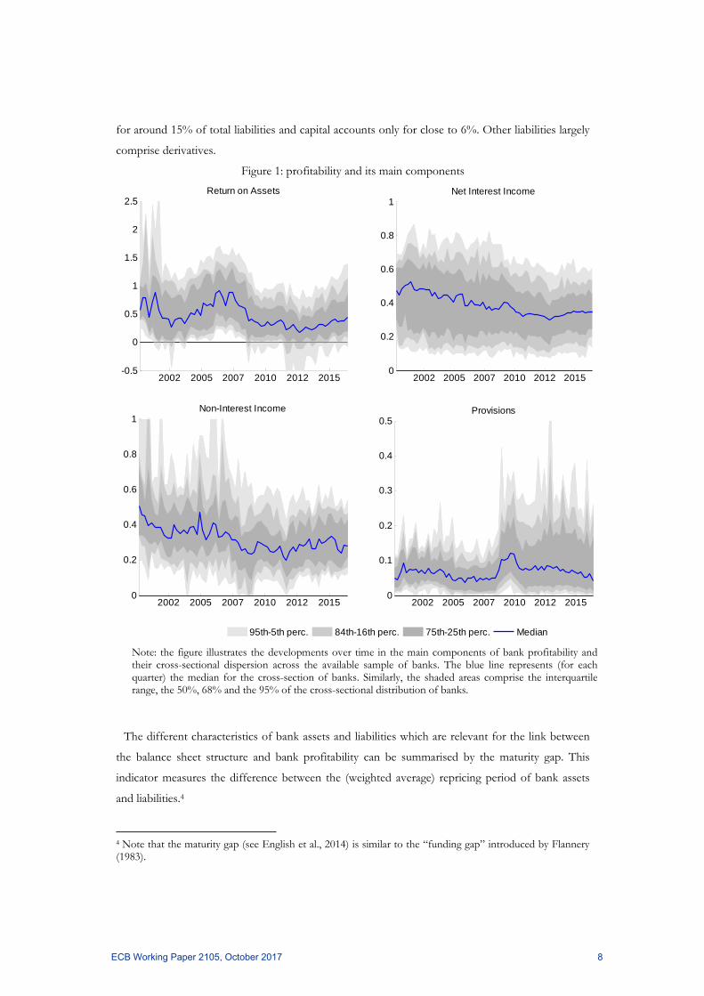
How exactly bank profitability is affected by interest rate changes depends on the relative effects

on its main components: net interest income, non-interest income, and provisions. Figure 1

illustrates the developments over time in bank profitability and its main components as well as their

cross-sectional dispersion. Bank profitability showed an increasing trend in the run-up to the

financial crisis, followed by a decline reflecting an abrupt increase in loan loss provisions. More

recently, there has been a gradual recovery of bank profitability supported by increasing net interest

income and declining provisions, reflecting higher credit quality thanks to the improved economic

outlook. The resilience of net interest income in the recent low interest rate environment reflected

savings in funding costs which more than offset lower interest income. In turn, interest income was

supported by increasing intermediation volumes.

In order to understand the link between monetary policy and interest rates, it is important to have

an overview of the main components of bank balance sheets in the euro area. Loans and advances

are the main component of total assets. For the euro area as a whole, total loans comprise around

60% of total assets, whereas loans to the non-financial private sector account for close to 40%.

Securities held represent 15-20% of the balance sheet, and about 2/3 of this item is comprised by

sovereign debt, with equity instruments accounting for around 10% of securities held by euro area

banks. Among the other assets, the main components are derivatives and cash and balances at

central banks. The largest component of the liability side is deposits, at around 60% of total assets,

of which about 60% are deposits from the non-financial private sector. Securities issued account


for around 15% of total liabilities and capital accounts only for close to 6%. Other liabilities largely

comprise derivatives.

Figure 1: profitability and its main components

Note: the figure illustrates the developments over time in the main components of bank profitability and their cross-sectional dispersion across the available sample of banks. The blue line represents (for each quarter) the median for the cross-section of banks. Similarly, the shaded areas comprise the interquartile range, the 50%, 68% and the 95% of the cross-sectional distribution of banks.

The different characteristics of bank assets and liabilities which are relevant for the link between

the balance sheet structure and bank profitability can be summarised by the maturity gap. This

indicator measures the difference between the (weighted average) repricing period of bank assets

and liabilities.4

4 Note that the maturity gap (see English et al., 2014) is similar to the “funding gap” introduced by Flannery (1983).

2002 2005 2007 2010 2012 2015-0.5

0

0.5

1

1.5

2

2.5Return on Assets

2002 2005 2007 2010 2012 20150

0.2

0.4

0.6

0.8

1Net Interest Income

2002 2005 2007 2010 2012 20150

0.2

0.4

0.6

0.8

1Non-Interest Income

2002 2005 2007 2010 2012 20150

0.1

0.2

0.3

0.4

0.5Provisions

95th-5th perc. 84th-16th perc. 75th-25th perc. Median


More formally, this indicator might be expressed as:

, , (1)

where denotes the weighted average repricing/maturity period (in months) of assets ( ),

which comprise loans to the non-financial private sector and debt securities held, whereas refers

to the repricing time of the liabilities , which in our case include deposits from the non-financial

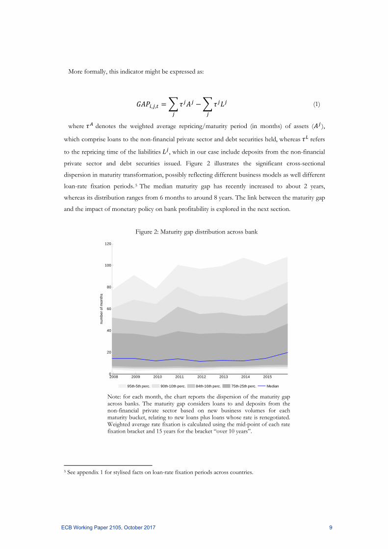
private sector and debt securities issued. Figure 2 illustrates the significant cross-sectional

dispersion in maturity transformation, possibly reflecting different business models as well different

loan-rate fixation periods. 5 The median maturity gap has recently increased to about 2 years,

whereas its distribution ranges from 6 months to around 8 years. The link between the maturity gap

and the impact of monetary policy on bank profitability is explored in the next section.

Figure 2: Maturity gap distribution across bank

Note: for each month, the chart reports the dispersion of the maturity gap across banks. The maturity gap considers loans to and deposits from the non-financial private sector based on new business volumes for each maturity bucket, relating to new loans plus loans whose rate is renegotiated. Weighted average rate fixation is calculated using the mid-point of each rate fixation bracket and 15 years for the bracket “over 10 years”.

5 See appendix 1 for stylised facts on loan-rate fixation periods across countries.

2008 2009 2010 2011 2012 2013 2014 20150

20

40

60

80

100

120

nu

mb

er

of m

on

ths

95th-5th perc. 90th-10th perc. 84th-16th perc. 75th-25th perc. Median


3 Exploiting the cross-section of banks In this section, the analysis concentrates on the impact of monetary policy on bank profitability

using accounting data for a cross-section of European banks. Return on assets is used as a measure

of profitability and regression analysis is employed to explore its drivers. In general, we examine the

role of monetary policy, the macroeconomic outlook and bank balance sheet characteristics. In

doing so, we rely on different datasets with different degrees of confidentiality/granularity. More

specifically, the analysis is carried out at quarterly frequency, matching different commercial

datasets available since the establishment of the euro area with different confidential ECB

proprietary datasets available at monthly and quarterly frequency over the period from June 2007 to

January 2017. Therefore, data availability explains why there may be differences in some empirical

specifications used in the analysis below.

3.1 Monetary policy and bank characteristics

In this subsection, we explore the link between monetary policy and bank profitability through

the lens of bank balance sheet information. We also analyse whether bank characteristics influence

the transmission of monetary policy actions to bank profitability.

The analysis focuses on the period from the start of 2000 to the end of 2016. We use quarterly

data collected from different sources. More specifically, we use three sets of variables. Financial

variables, such as the yield curve and the VIX, are taken from Datastream, while the country-

specific measure of expected default frequency (EDF) for non-financial firms is taken from

Moody’s Analytics. Macroeconomic indicators are taken from Eurostat (real GDP and HICP

inflation) and Consensus Economics (expected value of inflation and real GDP growth one year

ahead).

Finally, bank balance sheet data are taken from different commercial datasets – namely

Bankscope, SNL, Bloomberg and Capital IQ – with the aim of maximising the sample size. This

also makes it possible to check the consistency of the information provided by the four datasets

and hence minimise misreporting and outliers.

Descriptive statistics for the main variables used in the estimation are reported in Table 1.

For each variable, the table shows measures of central tendency and some selected percentiles

describing the frequency distribution of data; the total number of observations available for each

variable is given in the last column. The distribution across percentiles shows wide variation in the

data over the sample. This variation is visible for all groups of variables in the table. For the

regulatory capital ratio (i.e. the ratio of Tier 1 capital to risk-weighted assets), for example, the


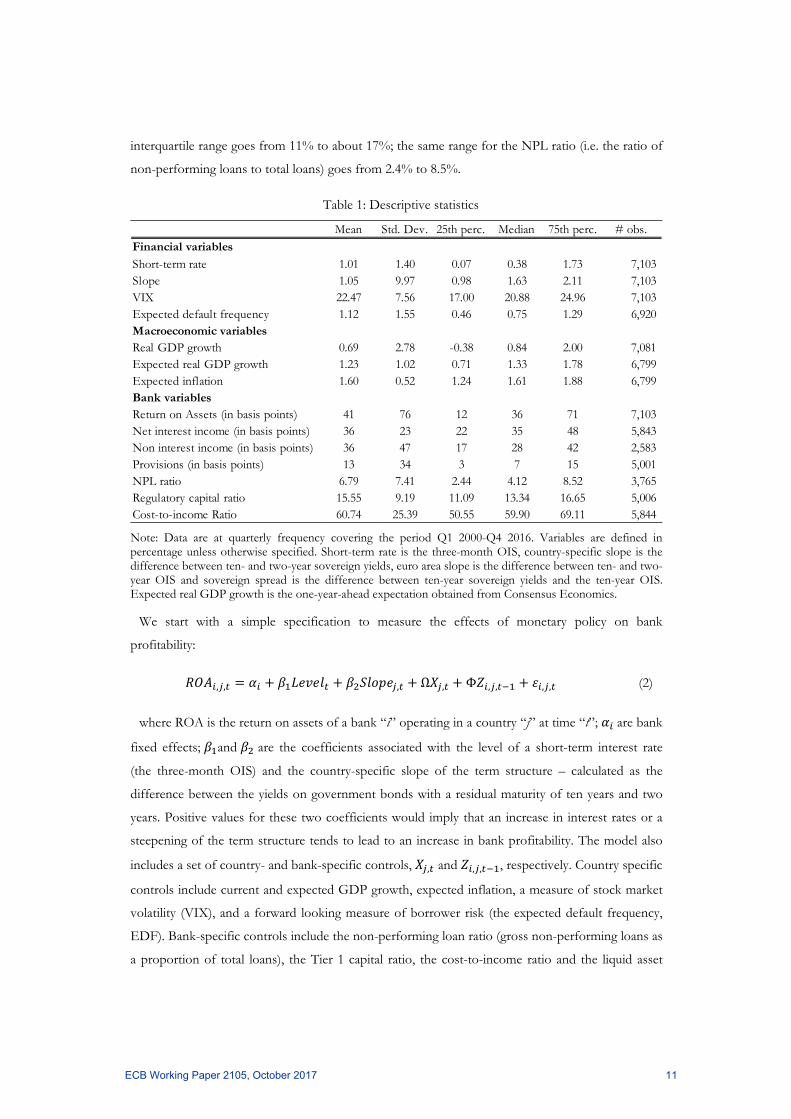
interquartile range goes from 11% to about 17%; the same range for the NPL ratio (i.e. the ratio of

non-performing loans to total loans) goes from 2.4% to 8.5%.

Table 1: Descriptive statistics

Note: Data are at quarterly frequency covering the period Q1 2000-Q4 2016. Variables are defined in percentage unless otherwise specified. Short-term rate is the three-month OIS, country-specific slope is the difference between ten- and two-year sovereign yields, euro area slope is the difference between ten- and two-year OIS and sovereign spread is the difference between ten-year sovereign yields and the ten-year OIS. Expected real GDP growth is the one-year-ahead expectation obtained from Consensus Economics.

We start with a simple specification to measure the effects of monetary policy on bank

profitability:

, , , Ω , Φ , , , , (2)

where ROA is the return on assets of a bank “i” operating in a country “j” at time “t”; are bank

fixed effects; and are the coefficients associated with the level of a short-term interest rate

(the three-month OIS) and the country-specific slope of the term structure – calculated as the

difference between the yields on government bonds with a residual maturity of ten years and two

years. Positive values for these two coefficients would imply that an increase in interest rates or a

steepening of the term structure tends to lead to an increase in bank profitability. The model also

includes a set of country- and bank-specific controls, , and , , , respectively. Country specific

controls include current and expected GDP growth, expected inflation, a measure of stock market

volatility (VIX), and a forward looking measure of borrower risk (the expected default frequency,

EDF). Bank-specific controls include the non-performing loan ratio (gross non-performing loans as

a proportion of total loans), the Tier 1 capital ratio, the cost-to-income ratio and the liquid asset

Mean Std. Dev. 25th perc. Median 75th perc. # obs.Financial variables

Short-term rate 1.01 1.40 0.07 0.38 1.73 7,103 Slope 1.05 9.97 0.98 1.63 2.11 7,103 VIX 22.47 7.56 17.00 20.88 24.96 7,103 Expected default frequency 1.12 1.55 0.46 0.75 1.29 6,920 Macroeconomic variablesReal GDP growth 0.69 2.78 -0.38 0.84 2.00 7,081 Expected real GDP growth 1.23 1.02 0.71 1.33 1.78 6,799 Expected inflation 1.60 0.52 1.24 1.61 1.88 6,799 Bank variablesReturn on Assets (in basis points) 41 76 12 36 71 7,103 Net interest income (in basis points) 36 23 22 35 48 5,843 Non interest income (in basis points) 36 47 17 28 42 2,583 Provisions (in basis points) 13 34 3 7 15 5,001 NPL ratio 6.79 7.41 2.44 4.12 8.52 3,765 Regulatory capital ratio 15.55 9.19 11.09 13.34 16.65 5,006 Cost-to-income Ratio 60.74 25.39 50.55 59.90 69.11 5,844


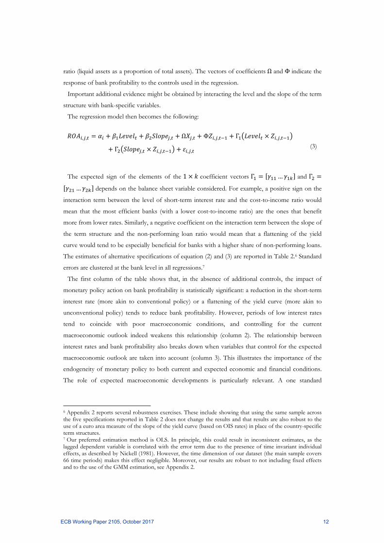
ratio (liquid assets as a proportion of total assets). The vectors of coefficients Ω and Φ indicate the

response of bank profitability to the controls used in the regression.

Important additional evidence might be obtained by interacting the level and the slope of the term

structure with bank-specific variables.

The regression model then becomes the following:

, , , Ω , Φ , , Γ , ,

Γ , , , , , (3)

The expected sign of the elements of the 1 coefficient vectors Γ … and Γ

… depends on the balance sheet variable considered. For example, a positive sign on the

interaction term between the level of short-term interest rate and the cost-to-income ratio would

mean that the most efficient banks (with a lower cost-to-income ratio) are the ones that benefit

more from lower rates. Similarly, a negative coefficient on the interaction term between the slope of

the term structure and the non-performing loan ratio would mean that a flattening of the yield

curve would tend to be especially beneficial for banks with a higher share of non-performing loans.

The estimates of alternative specifications of equation (2) and (3) are reported in Table 2.6 Standard

errors are clustered at the bank level in all regressions.7

The first column of the table shows that, in the absence of additional controls, the impact of

monetary policy action on bank profitability is statistically significant: a reduction in the short-term

interest rate (more akin to conventional policy) or a flattening of the yield curve (more akin to

unconventional policy) tends to reduce bank profitability. However, periods of low interest rates

tend to coincide with poor macroeconomic conditions, and controlling for the current

macroeconomic outlook indeed weakens this relationship (column 2). The relationship between

interest rates and bank profitability also breaks down when variables that control for the expected

macroeconomic outlook are taken into account (column 3). This illustrates the importance of the

endogeneity of monetary policy to both current and expected economic and financial conditions.

The role of expected macroeconomic developments is particularly relevant. A one standard

6 Appendix 2 reports several robustness exercises. These include showing that using the same sample across the five specifications reported in Table 2 does not change the results and that results are also robust to the use of a euro area measure of the slope of the yield curve (based on OIS rates) in place of the country-specific term structures. 7 Our preferred estimation method is OLS. In principle, this could result in inconsistent estimates, as the lagged dependent variable is correlated with the error term due to the presence of time invariant individual effects, as described by Nickell (1981). However, the time dimension of our dataset (the main sample covers 66 time periods) makes this effect negligible. Moreover, our results are robust to not including fixed effects and to the use of the GMM estimation, see Appendix 2.


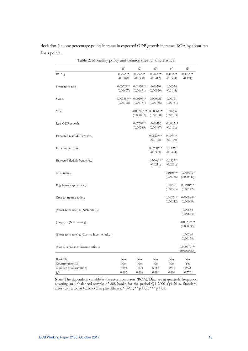
deviation (i.e. one percentage point) increase in expected GDP growth increases ROA by about ten

basis points.

Table 2: Monetary policy and balance sheet characteristics

Note: The dependent variable is the return on assets (ROA). Data are at quarterly frequency covering an unbalanced sample of 288 banks for the period Q1 2000–Q4 2016. Standard errors clustered at bank level in parentheses: * p<.1, ** p<.05, *** p<.01.

(1) (2) (3) (4) (5)

ROAt-1 0.585*** 0.556*** 0.506*** 0.413*** 0.425***(0.0348) (0.0330) (0.0412) (0.0584) (0.121)

Short-term ratet 0.0332*** 0.0199*** -0.00209 0.00374(0.00667) (0.00671) (0.00820) (0.0148)

Slopet 0.00338*** 0.00293** 0.000631 0.00161(0.00128) (0.00131) (0.00136) (0.00151)

VIXt -0.00285*** 0.00261** 0.00266(0.000718) (0.00108) (0.00183)

Real GDP growtht 0.0238*** -0.00496 -0.000249(0.00589) (0.00487) (0.0101)

Expected real GDP growtht 0.0823*** 0.107***(0.0108) (0.0169)

Expected inflationt 0.0960*** 0.112**(0.0303) (0.0494)

Expected default frequencyt -0.0568*** -0.0557**(0.0211) (0.0261)

NPL ratiot-1 -0.0108*** -0.000979*(0.00356) (0.000440)

Regulatory capital ratiot-1 0.00581 0.0218***(0.00385) (0.00772)

Cost-to-income ratiot-1 -0.00251** 0.000884*(0.00112) (0.00049)

(Short-term ratet) x (NPL ratiot-1) 0.00634(0.00644)

(Slopet) x (NPL ratiot-1) -0.00233***(0.000395)

(Short-term ratet) x (Cost-to-income ratiot-1) 0.00204(0.00134)

(Slopet) x (Cost-to-income ratiot-1) 0.000277***(0.0000768)

Bank FE Yes Yes Yes Yes YesCountry*time FE No No No No YesNumber of observations 7,093 7,071 6,768 2974 2992

R2 0.683 0.688 0.699 0.604 0.773


The logic behind this result is that a better expected macroeconomic outlook could increase

current loan demand by stimulating investment which, in the euro area, is largely funded via bank

intermediation. On the supply side, banks might be induced to increase their lending to the non-

financial private sector as the improved economic outlook will translate into increased company

and household income, and hence lower credit risk. Also, when including bank-specific variables,

an average bank’s profitability is not found to react to changes in the level or the slope of the yield

curve – see column 4, our baseline specification. Important bank-specific control variables are the

NPL ratio, the cost-to-income ratio and the regulatory capital ratio. Banks with a higher NPL ratio

tend to demonstrate lower profitability: a one standard deviation (i.e. 7.4 percentage points)

increase in the NPL ratio reduces ROA by 8 basis points. This result is intuitive as bad loans do not

generate income and lead to costs associated with provisions for credit losses as well as operational

costs associated with their management and resolution. In line with previous studies (e.g. Alexiou

and Sofoklis, 2009; Athanasoglou et al., 2008; Dietrich and Wanzenried, 2011; García-Herrero et al.,

2009; Pasiouras and Kosmidou, 2007), we find that cost efficiency has a positive and highly

significant impact on profitability: a one standard deviation (i.e. 25 percentage point) increase in the

cost-to-income ratio reduces ROA by 6 basis points. This relationship shows that operational

efficiency is a major avenue to explore in order to improve bank profitability.

Finally, we test whether the effect of monetary policy on profitability depends on the cost

efficiency or the credit quality of a bank’s loan portfolio. We find a negative value for the

interaction terms between the level and slope of the term structure and the NPL ratio, implying that

the higher the NPL, the more positive the impact of monetary policy easing on profitability. There

could be different reasons that explain this. First, NPL are non-income producing assets that still

need to be funded. This means that lower interest rates, by decreasing funding costs, decrease the

cost of holding NPL. Second, policy easing would decrease the cost of servicing debt, thereby

exerting a positive influence on borrowers’ ability to honour their commitments (and their

probability of default).

We also find that the impact of monetary policy on bank profitability depends on the relative

(operational) efficiency of a given bank. The coefficients on the interaction terms with the level and

the slope of the term structure are both positive, suggesting that the effect of monetary policy

easing on profitability is more positive in relative terms for banks with a lower cost-to-income ratio,

i.e. with greater operational efficiency.

3.2 Keeping interest rates low for long

The results presented above indicate that changes in short-term rates or in the slope of the yield

curve do not significantly influence bank profitability once macroeconomic and bank-specific

controls are appropriately taken into account. Nonetheless, there might be adverse effects on bank


profitability if rates remain low for a long period of time. Indeed, following a decrease in interest

rates, net interest margins are at first shielded due to the typically faster repricing of the outstanding

amount of liabilities as compared to assets. Since assets tend to be longer term, changes in the

interest rates applied on new business take longer to be reflected in the outstanding amount of

loans. A protracted low interest rate environment could therefore be expected to be more

detrimental for banks.

This subsection presents a test for this hypothesis within the regression framework.

In principle, there are various methods to capture the heterogeneous effects of monetary policy in

a protracted low interest rate environment. Claessens et al. (2017), for example, identify such an

environment by constructing a variable that counts the number of periods in which a reference

interest rate is lower than a fixed threshold (1.25% for the three-month rate, in their case). Along

these lines, the duration of the low interest rate environment might be captured by a variable that

counts the periods when the rate on marginal refinancing operations (MRO) or the interbank

overnight rate (EONIA) has been below a fixed threshold. In these cases, however, the results will

depend on the particular (arbitrary) value used for the threshold. In order to avoid the need to

define an ad hoc threshold, we construct a variable, defined as the sum of consecutive quarters in

which residuals from an estimated Taylor rule are negative. The Taylor rule uses the three-month

overnight index swap (OIS) rate as proxy for the monetary policy instrument and includes

expectations for future inflation and for GDP growth one year ahead. The identification of the low-

for-long period based on Taylor residuals is therefore less arbitrary.

In practice, we add three variables measuring the low-for-long to our baseline specification and

present the results in Table 3. Specifically, “Low for long . ” and “Low for

long . ” count the number of consecutive quarters in which the MRO and EONIA

rates are below 1.5% and 1.25%, respectively (the associated results are in column 2 and 3); “Low

for long (Taylor rule)” is a variable that counts the number of consecutive quarters in which

residuals of the forward-looking Taylor rule are negative (results are in column 4).8

Comparing column 1 with columns 2 to 4 of the table shows that results concerning the impact

on profitability of changes in yields, the macroeconomic environment and bank-specific

characteristics are robust to the inclusion of the low-for-long variable in the model specification.

Importantly, the coefficients for the low-for-long measures reported in columns 2 to 4 are all

negative and statistically significant, suggesting that keeping rates low for an extend period of time

might have negative consequences for bank profitability.

8 Figure A1.4 in Appendix 1 displays the measures of low for long used in the estimations.


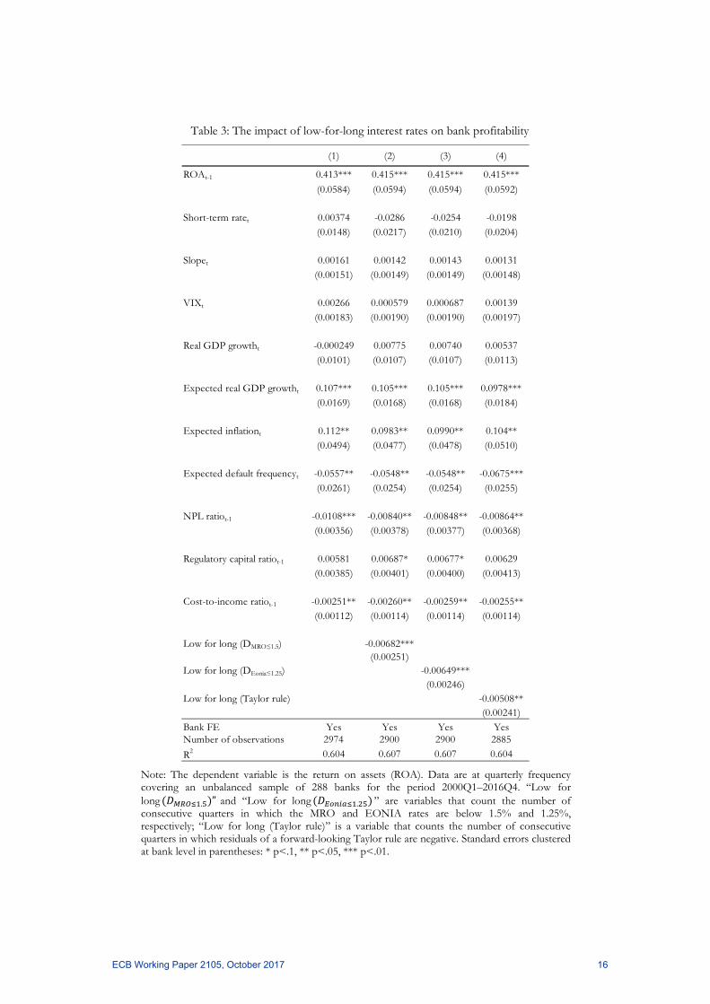
Table 3: The impact of low-for-long interest rates on bank profitability

Note: The dependent variable is the return on assets (ROA). Data are at quarterly frequency covering an unbalanced sample of 288 banks for the period 2000Q1–2016Q4. “Low for long . ” and “Low for long . ” are variables that count the number of consecutive quarters in which the MRO and EONIA rates are below 1.5% and 1.25%, respectively; “Low for long (Taylor rule)” is a variable that counts the number of consecutive quarters in which residuals of a forward-looking Taylor rule are negative. Standard errors clustered at bank level in parentheses: * p<.1, ** p<.05, *** p<.01.

(1) (2) (3) (4)

ROAt-1 0.413*** 0.415*** 0.415*** 0.415***

(0.0584) (0.0594) (0.0594) (0.0592)

Short-term ratet 0.00374 -0.0286 -0.0254 -0.0198(0.0148) (0.0217) (0.0210) (0.0204)

Slopet 0.00161 0.00142 0.00143 0.00131(0.00151) (0.00149) (0.00149) (0.00148)

VIXt 0.00266 0.000579 0.000687 0.00139(0.00183) (0.00190) (0.00190) (0.00197)

Real GDP growtht -0.000249 0.00775 0.00740 0.00537(0.0101) (0.0107) (0.0107) (0.0113)

Expected real GDP growtht 0.107*** 0.105*** 0.105*** 0.0978***(0.0169) (0.0168) (0.0168) (0.0184)

Expected inflationt 0.112** 0.0983** 0.0990** 0.104**(0.0494) (0.0477) (0.0478) (0.0510)

Expected default frequencyt -0.0557** -0.0548** -0.0548** -0.0675***(0.0261) (0.0254) (0.0254) (0.0255)

NPL ratiot-1 -0.0108*** -0.00840** -0.00848** -0.00864**(0.00356) (0.00378) (0.00377) (0.00368)

Regulatory capital ratiot-1 0.00581 0.00687* 0.00677* 0.00629(0.00385) (0.00401) (0.00400) (0.00413)

Cost-to-income ratiot-1 -0.00251** -0.00260** -0.00259** -0.00255**(0.00112) (0.00114) (0.00114) (0.00114)

Low for long (DMRO≤1.5) -0.00682***(0.00251)

Low for long (DEonia≤1.25) -0.00649***(0.00246)

Low for long (Taylor rule) -0.00508**(0.00241)

Bank FE Yes Yes Yes YesNumber of observations 2974 2900 2900 2885

R2 0.604 0.607 0.607 0.604


These results are broadly in line with the evidence reported by Claessens et al. (2017) for a large

cross-section of banks covering several countries. However, the relatively small size of the

coefficients of the low-for-long variables indicates that it would take a relatively long period of time

for a monetary policy easing to exert a significant adverse effect on bank profitability. In addition,

the materialisation of the negative consequences for bank profitability would be offset by the

impact of low rates on real economic activity.

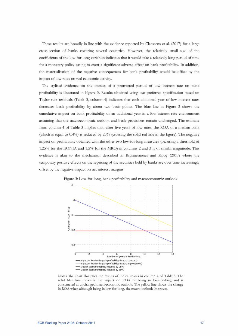
The stylised evidence on the impact of a protracted period of low interest rate on bank

profitability is illustrated in Figure 3. Results obtained using our preferred specification based on

Taylor rule residuals (Table 3, column 4) indicates that each additional year of low interest rates

decreases bank profitability by about two basis points. The blue line in Figure 3 shows the

cumulative impact on bank profitability of an additional year in a low interest rate environment

assuming that the macroeconomic outlook and bank provisions remain unchanged. The estimate

from column 4 of Table 3 implies that, after five years of low rates, the ROA of a median bank

(which is equal to 0.4%) is reduced by 25% (crossing the solid red line in the figure). The negative

impact on profitability obtained with the other two low-for-long measures (i.e. using a threshold of

1.25% for the EONIA and 1.5% for the MRO) in columns 2 and 3 is of similar magnitude. This

evidence is akin to the mechanism described in Brunnermeier and Koby (2017) where the

temporary positive effects on the repricing of the securities held by banks are over time increasingly

offset by the negative impact on net interest margins.

Figure 3: Low-for-long, bank profitability and macroeconomic outlook

Notes: the chart illustrates the results of the estimates in column 4 of Table 3. The solid blue line indicates the impact on ROA of being in low-for-long and is constructed at unchanged macroeconomic outlook. The yellow line shows the change in ROA when although being in low-for-long, the macro outlook improves.

0 2 4 6 8 10 12 14

-0.3

-0.2

-0.1

0

0.1

Number of years in low-for-long

Cha

nge

in R

OA

- in

pp

Impact of low-for-long on profitability (Macro constant)Impact of low-for-long on profitability (Macro improvement)Median bank profitability reduced by 25%Median bank profitability reduced by 50%


The estimated impact can, however, be substantially different when the endogenous reaction of

the macro variables associated with the low interest rate environment is taken into account. This is

illustrated by the yellow line in Figure 3: a 1pp increase in the expected GDP (associated with an

increase in bank profitability of about 10 basis points) would shift the blue line outward thereby

contributing to a significant delay in the materialisation of the negative consequences for bank

profitability associated with a low-for-long environment. For the first five years the change in

expected GDP more than offsets the negative impact on profitability linked to the low-for-long; it

would then take about ten years (twice as long as in the previous case) to reduce the profitability of

the median bank by 25%. Overall, the adverse impact of a protracted period of low rates on

profitability is likely to be offset by the respective impact on loan loss provisions and

intermediation volumes, a mechanism not envisaged in Brunnermeier and Koby (2017) and further

explored in the next subsection.

3.3 Components of bank profitability

In order to empirically document the channels through which monetary policy actions are

transmitted to bank profitability, the analysis presented in this section singles out the impact of

changes in interest rates on the main components of profitability.

The impact on net interest income works via a price channel, i.e. the components of the net interest

margin, and via a quantity channel, which is more closely related to the positive impact of the low

interest environment on aggregated demand. The second component is non-interest income, driven

mainly by capital gains, fees and commissions. This component plays a special role when QE

policies are implemented as the impact on asset values in financial markets might generate sizeable

capital gains. The third component is provisions. This is related to the macro effects of the policies

and the associated impact on borrowers’ credit quality.

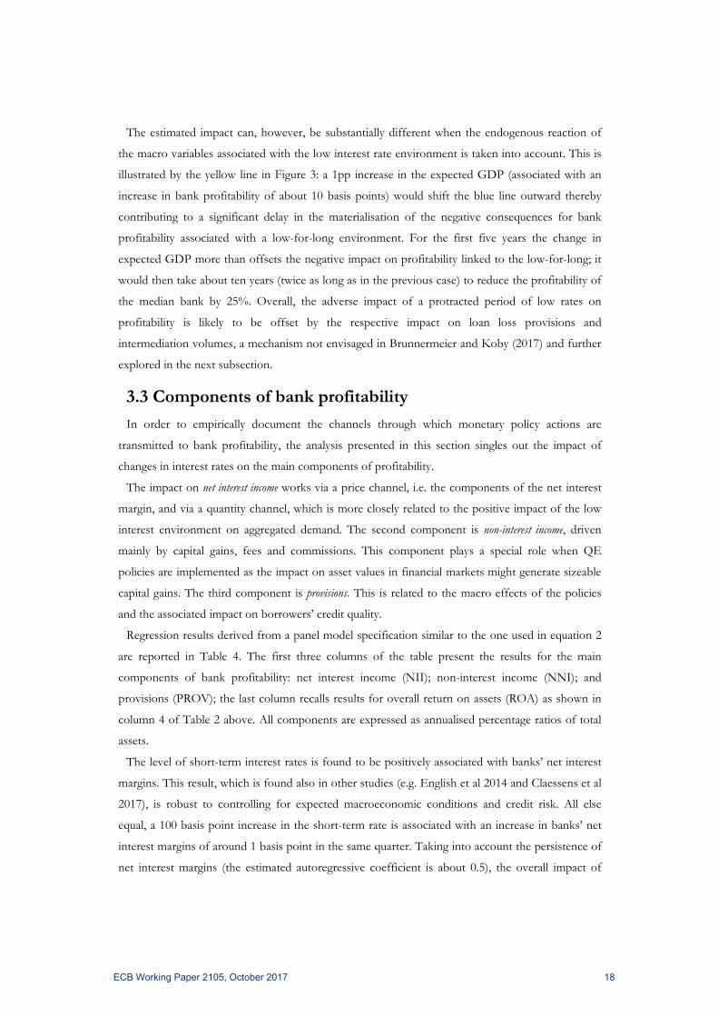
Regression results derived from a panel model specification similar to the one used in equation 2

are reported in Table 4. The first three columns of the table present the results for the main

components of bank profitability: net interest income (NII); non-interest income (NNI); and

provisions (PROV); the last column recalls results for overall return on assets (ROA) as shown in

column 4 of Table 2 above. All components are expressed as annualised percentage ratios of total

assets.

The level of short-term interest rates is found to be positively associated with banks’ net interest

margins. This result, which is found also in other studies (e.g. English et al 2014 and Claessens et al

2017), is robust to controlling for expected macroeconomic conditions and credit risk. All else

equal, a 100 basis point increase in the short-term rate is associated with an increase in banks’ net

interest margins of around 1 basis point in the same quarter. Taking into account the persistence of

net interest margins (the estimated autoregressive coefficient is about 0.5), the overall impact of


such a shock would be 2.5 basis points, which corresponds to around 7% of the mean of the net

interest margin. Net interest margins are also found to be positively associated with economic

growth. Conversely, low asset quality and high cost to income ratios tend to compress net interest

margins.

Table 4: Profitability components and monetary policy

Note: Dependent variables: NII = net interest income as a percent of assets; NNI = non-interest

income as a percent of assets; PROV= provisions; ROA = return on assets. denote the lagged dependent variables. Data are at quarterly frequency covering an unbalanced sample of 288 banks for the period Q1 2000–Q4 2016. Standard errors clustered at bank level in parentheses: * p<.1, ** p<.05, *** p<.01.

(1) (2) (3) (4)NII NNI PROV ROA

Yt-1 0.533** 0.0260 0.0665 0.413***(0.1851) (0.0353) (0.0568) (0.0584)

Short-term ratet 0.0089** -0.00817 0.0104* 0.00374(0.00409) (0.0112) (0.00595) (0.0148)

Slopet 0.000269 -0.00101 0.000666* 0.00161(0.000225) (0.00129) (0.000336) (0.00151)

VIXt 0.000549 -0.00153* 0.00239*** 0.00266(0.000373) (0.000845) (0.000788) (0.00183)

Real GDP growtht 0.00248** 0.00703 0.000505 -0.000249(0.00114) (0.00591) (0.00201) (0.0101)

Expected real GDP growtht 0.00203 0.0312*** -0.0476*** 0.107***(0.00349) (0.00919) (0.0128) (0.0169)

Expected inflationt 0.00150 0.00734 -0.0526** 0.112**(0.00822) (0.0141) (0.0210) (0.0494)

Expected default frequencyt -0.00287 -0.0217* 0.0335*** -0.0557**(0.00389) (0.0123) (0.0108) (0.0261)

NPL ratiot-1 -0.00413*** 0.00351 0.00871*** -0.0108***(0.00138) (0.00279) (0.00243) (0.00356)

Regulatory capital ratiot-1 0.00177 -0.00372 -0.00495*** 0.00581(0.00111) (0.00513) (0.00161) (0.00385)

Cost-to-income ratiot-1 -0.000488*** -0.000207 0.000317 -0.00251**(0.000154) (0.000406) (0.000424) (0.00112)

Bank FE YES YES YES YESNumber of observations 2794 1758 2754 2974R2 0.740 0.317 0.399 0.604


Results for non-interest income are less clear-cut: no significant relationship is found with the

level or slope of interest rates. The main determinants of non-interest income are changes in the

valuation of securities held and fee and commission income. The first determinant in particular,

should in principle benefit from a decline in interest rates, as lower yields are reflected in higher

asset prices. It is however, important to note that while changes in the valuation of securities held

by banks affect their economic value, they are reflected in the profit and loss account only if the

securities are accounted at market values or if the capital gain/loss is realised. Since the share of

securities held at market values is relatively small (see LHS panel of Figure A1.3) it is not surprising

that the estimated coefficient is not statistically significant.

Costs associated with loan loss provisions increase (decrease) following an upward (downward)

shift or a steepening (flattening) of the yield curve. As discussed in Section 2 above, this is likely to

reflect the fact that lower interest rates allow for a decrease in borrowers’ probability of default and

in the associated loss given default. Importantly, provisions are significantly affected by expected

developments in economic growth and default frequencies. A one standard deviation (or 1.02

percentage point) increase in expected GDP leads to a reduction in provisions of 5 basis points,

which corresponds to around one third of the provisions observed at the mean. An analogous

decrease in the expected default frequency (1 standard deviation or 1.28%) leads to a similar impact

on provisions.

3.4 The role of maturity transformation

In this subsection, we explore the role played by maturity transformation in the relationship

between monetary policy and bank profitability. We do so by augmenting the regression model

expressed in equation 3 with a bank-specific measure of the difference between the average

maturity of its assets and liabilities: the maturity gap (as defined in equation 1). This variable could

play an important role in the transmission of changes in interest rates to bank profitability. For

example, a positive sign on the interaction term between the slope of the yield curve and the

maturity gap would mean that banks engaging more heavily in maturity transformation tend to

benefit more in relative terms from a steepening of the term structure.

In order to obtain information on the average maturity of the different balance sheet items, we

use bank data on income and balance sheet characteristics retrieved by matching data from S&P

Global Market Intelligence (formerly known as SNL Financial) with the iBSI (individual Balance

Sheet Information), a proprietary dataset on bank balance sheet information available at a monthly

frequency and maintained at the ECB. Given data limitations, the empirical analysis focuses on the

period running from mid-2007 to end-2016. Importantly, the sample of banks covered by the

dataset is chosen so as to be representative of the overall banking sector, thereby reflecting different


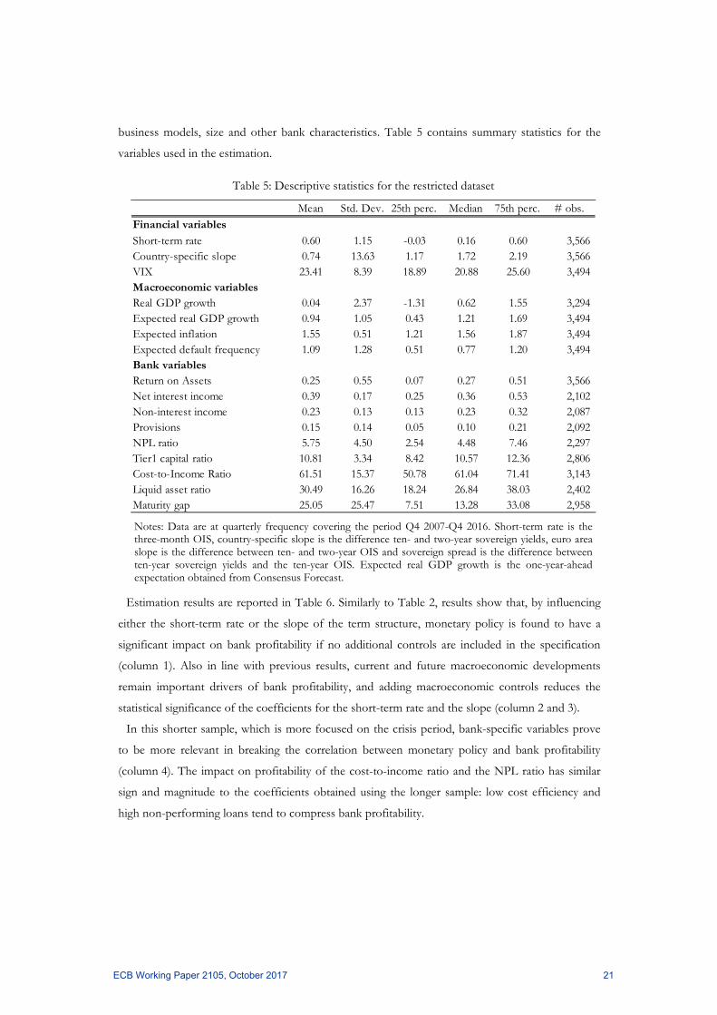
business models, size and other bank characteristics. Table 5 contains summary statistics for the

variables used in the estimation.

Table 5: Descriptive statistics for the restricted dataset

Notes: Data are at quarterly frequency covering the period Q4 2007-Q4 2016. Short-term rate is the three-month OIS, country-specific slope is the difference ten- and two-year sovereign yields, euro area slope is the difference between ten- and two-year OIS and sovereign spread is the difference between ten-year sovereign yields and the ten-year OIS. Expected real GDP growth is the one-year-ahead expectation obtained from Consensus Forecast.

Estimation results are reported in Table 6. Similarly to Table 2, results show that, by influencing

either the short-term rate or the slope of the term structure, monetary policy is found to have a

significant impact on bank profitability if no additional controls are included in the specification

(column 1). Also in line with previous results, current and future macroeconomic developments

remain important drivers of bank profitability, and adding macroeconomic controls reduces the

statistical significance of the coefficients for the short-term rate and the slope (column 2 and 3).

In this shorter sample, which is more focused on the crisis period, bank-specific variables prove

to be more relevant in breaking the correlation between monetary policy and bank profitability

(column 4). The impact on profitability of the cost-to-income ratio and the NPL ratio has similar

sign and magnitude to the coefficients obtained using the longer sample: low cost efficiency and

high non-performing loans tend to compress bank profitability.

Mean Std. Dev. 25th perc. Median 75th perc. # obs.Financial variables

Short-term rate 0.60 1.15 -0.03 0.16 0.60 3,566 Country-specific slope 0.74 13.63 1.17 1.72 2.19 3,566 VIX 23.41 8.39 18.89 20.88 25.60 3,494 Macroeconomic variablesReal GDP growth 0.04 2.37 -1.31 0.62 1.55 3,294 Expected real GDP growth 0.94 1.05 0.43 1.21 1.69 3,494 Expected inflation 1.55 0.51 1.21 1.56 1.87 3,494 Expected default frequency 1.09 1.28 0.51 0.77 1.20 3,494 Bank variablesReturn on Assets 0.25 0.55 0.07 0.27 0.51 3,566 Net interest income 0.39 0.17 0.25 0.36 0.53 2,102 Non-interest income 0.23 0.13 0.13 0.23 0.32 2,087 Provisions 0.15 0.14 0.05 0.10 0.21 2,092 NPL ratio 5.75 4.50 2.54 4.48 7.46 2,297 Tier1 capital ratio 10.81 3.34 8.42 10.57 12.36 2,806 Cost-to-Income Ratio 61.51 15.37 50.78 61.04 71.41 3,143 Liquid asset ratio 30.49 16.26 18.24 26.84 38.03 2,402 Maturity gap 25.05 25.47 7.51 13.28 33.08 2,958


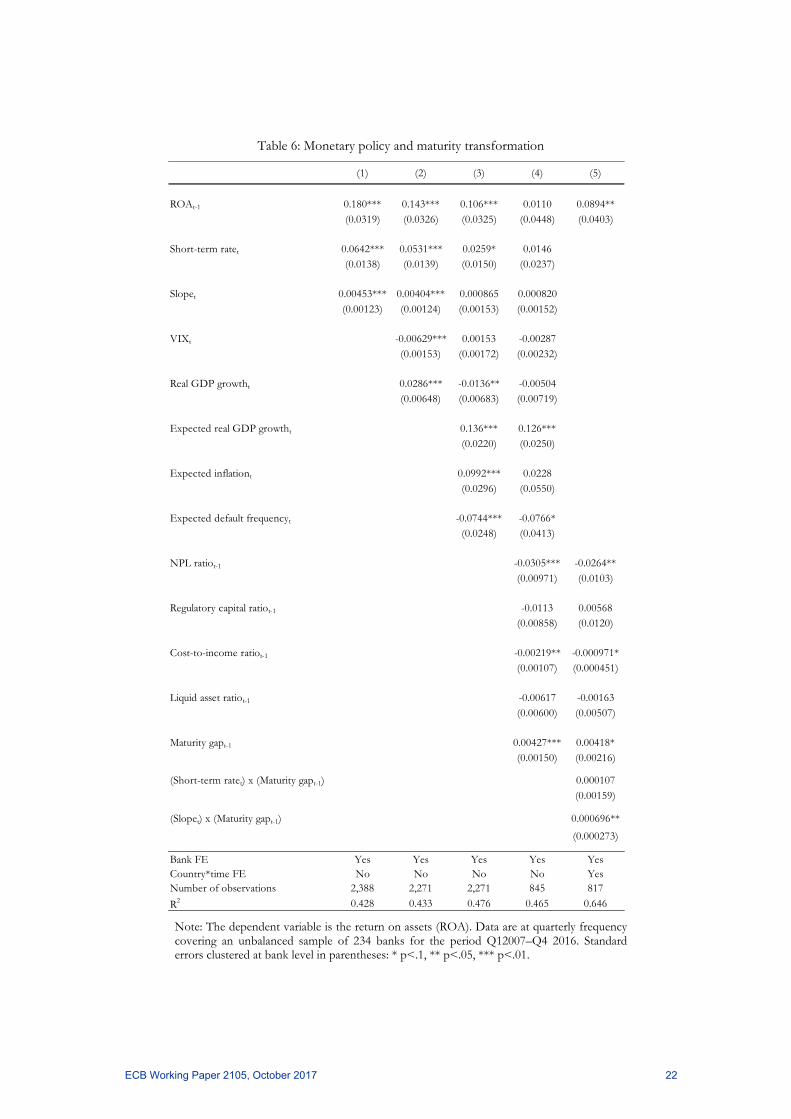
Table 6: Monetary policy and maturity transformation

Note: The dependent variable is the return on assets (ROA). Data are at quarterly frequency covering an unbalanced sample of 234 banks for the period Q12007–Q4 2016. Standard errors clustered at bank level in parentheses: * p<.1, ** p<.05, *** p<.01.

(1) (2) (3) (4) (5)

ROAt-1 0.180*** 0.143*** 0.106*** 0.0110 0.0894**(0.0319) (0.0326) (0.0325) (0.0448) (0.0403)

Short-term ratet 0.0642*** 0.0531*** 0.0259* 0.0146(0.0138) (0.0139) (0.0150) (0.0237)

Slopet 0.00453*** 0.00404*** 0.000865 0.000820(0.00123) (0.00124) (0.00153) (0.00152)

VIXt -0.00629*** 0.00153 -0.00287(0.00153) (0.00172) (0.00232)

Real GDP growtht 0.0286*** -0.0136** -0.00504(0.00648) (0.00683) (0.00719)


Expected inflationt 0.0992*** 0.0228(0.0296) (0.0550)

Expected default frequencyt -0.0744*** -0.0766*(0.0248) (0.0413)

NPL ratiot-1 -0.0305*** -0.0264**(0.00971) (0.0103)

Regulatory capital ratiot-1 -0.0113 0.00568(0.00858) (0.0120)

Cost-to-income ratiot-1 -0.00219** -0.000971*(0.00107) (0.000451)

Liquid asset ratiot-1 -0.00617 -0.00163(0.00600) (0.00507)

Maturity gapt-1 0.00427*** 0.00418*(0.00150) (0.00216)

(Short-term ratet) x (Maturity gapt-1) 0.000107(0.00159)

(Slopet) x (Maturity gapt-1) 0.000696**

(0.000273)

Bank FE Yes Yes Yes Yes YesCountry*time FE No No No No YesNumber of observations 2,388 2,271 2,271 845 817

R2 0.428 0.433 0.476 0.465 0.646


The positive coefficient on the maturity gap reflects the idea that, all other things being equal,

increased maturity transformation translates into higher profitability (see English et al., 2014). An

average bank will see its ROA increase by 11 basis points by increasing its maturity gap by one

standard deviation (i.e. 25 months).

Moreover, we investigate whether the impact of changes in the level and the slope of the term

structure depend on the maturity gap. The results in column 5 show that the profitability of banks

that engage more heavily in maturity transformation has a more positive reaction to a steepening of

the yield curve in relative terms. A bank with a maturity gap that is one standard deviation above

the sample average sees its profitability increase by two basis points in response to a 100 basis point

steepening of the yield curve.

In principle, the impact of monetary policy action on bank profitability through maturity

transformation would be mitigated if banks used derivatives to hedge exposures to interest rate risk.

Recent evidence by Begenau et al. (2015), however, suggests that the extent to which US banks use

interest rate derivatives to hedge exposures to interest rate is limited. For the euro area, Hoffmann

et al. (2017) find that banks use derivatives to reduce their banking book exposures to interest rate

risk by 25%, on average. This suggests that not accounting explicitly for hedging activities should

not lead to a significant bias in our estimates.

4 Evidence from a stylised macro model This section focuses on the impact on bank profitability of a monetary policy easing through the

lens of a dynamic model estimated at euro area level. The model is Bayesian vector-autoregression

(BVAR) thought to capture the main channels through which monetary policy affect bank

profitability. The variables included in the model are: return on assets (ROA), net interest income

(NII), non-interest income (NNI), loan loss provisions (Provisions), lending rates to non-financial

corporations (NFC), loan volumes to NFC, real GDP, HICP inflation, and interest rates with a

remaining maturity of 1-day (i.e. the Eonia rate), 5-year, and 10-year. The variables enter the VAR

in log-levels (or levels for variables already expressed in terms of rates) with 5 lags, for a sample

period ranging from January 1999 to March 2017. For the estimation of the VAR, we address the

curse of dimensionality problem by using Bayesian shrinkage, as suggested in De Mol et al. (2008).

In more detail, we use Normal-Inverse Wishart prior distributions: we impose the so-called

Minnesota prior, according to which each variable follows a random walk process, possibly with

drift (Litterman, 1979). Moreover, we impose two sets of prior distributions on the sum of the

coefficients of the VAR model: the “sum-of-coefficients” prior, originally proposed by Doan et al.

(1984), and an additional prior that was introduced by Sims (1993), known as the “dummy-initial-

observation” prior. The hyper-parameters controlling for the informativeness of the prior


distributions are treated, as suggested in Giannone et al. (2015), as random variables and are drawn

from their posterior distribution, so that we also account for the uncertainty surrounding the prior

set-up in our evaluation.

In order to capture the impact of monetary policy in a low interest rate environment we simulate

the response of the variables included in the model to a policy easing shock that resembles the

effect of a quantitative easing (QE) policy on the term structure of interest rates, i.e. the effects are

increasing in the remaining maturity of the underlying bonds (see Altavilla, Carboni, Motto, 2015).

More precisely, the easing shock consists of a decrease in the 10-year yields of 100bps with a

simultaneous smaller reduction on the 5-year and the Eonia amounting to 40 and 5 basis points,

respectively. The shock is temporary and dies out over time with a decay that is assumed to be the

same across maturities and fixed at 0.9.

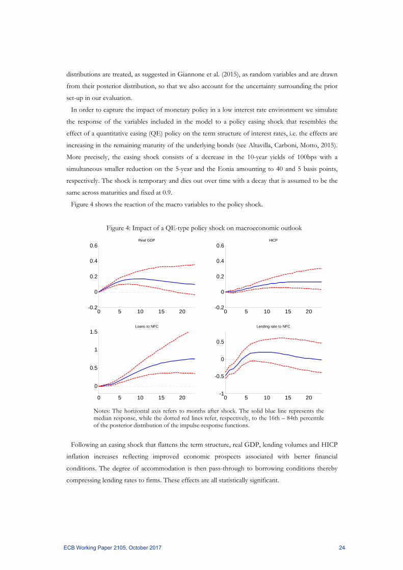
Figure 4 shows the reaction of the macro variables to the policy shock.

Figure 4: Impact of a QE-type policy shock on macroeconomic outlook

Notes: The horizontal axis refers to months after shock. The solid blue line represents the median response, while the dotted red lines refer, respectively, to the 16th – 84th percentile of the posterior distribution of the impulse-response functions.

Following an easing shock that flattens the term structure, real GDP, lending volumes and HICP

inflation increases reflecting improved economic prospects associated with better financial

conditions. The degree of accommodation is then pass-through to borrowing conditions thereby

compressing lending rates to firms. These effects are all statistically significant.

0 5 10 15 20-0.2

0

0.2

0.4

0.6Real GDP

0 5 10 15 20-0.2

0

0.2

0.4

0.6HICP

0 5 10 15 20

0

0.5

1

1.5Loans to NFC

0 5 10 15 20-1

-0.5

0

0.5

Lending rate to NFC


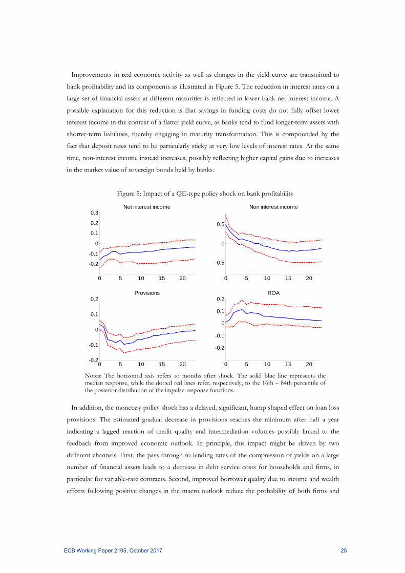
Improvements in real economic activity as well as changes in the yield curve are transmitted to

bank profitability and its components as illustrated in Figure 5. The reduction in interest rates on a

large set of financial assets at different maturities is reflected in lower bank net interest income. A

possible explanation for this reduction is that savings in funding costs do not fully offset lower

interest income in the context of a flatter yield curve, as banks tend to fund longer-term assets with

shorter-term liabilities, thereby engaging in maturity transformation. This is compounded by the

fact that deposit rates tend to be particularly sticky at very low levels of interest rates. At the same

time, non-interest income instead increases, possibly reflecting higher capital gains due to increases

in the market value of sovereign bonds held by banks.

Figure 5: Impact of a QE-type policy shock on bank profitability

Notes: The horizontal axis refers to months after shock. The solid blue line represents the median response, while the dotted red lines refer, respectively, to the 16th – 84th percentile of the posterior distribution of the impulse-response functions.

In addition, the monetary policy shock has a delayed, significant, hump shaped effect on loan loss

provisions. The estimated gradual decrease in provisions reaches the minimum after half a year

indicating a lagged reaction of credit quality and intermediation volumes possibly linked to the

feedback from improved economic outlook. In principle, this impact might be driven by two

different channels. First, the pass-through to lending rates of the compression of yields on a large

number of financial assets leads to a decrease in debt service costs for households and firms, in

particular for variable-rate contracts. Second, improved borrower quality due to income and wealth

effects following positive changes in the macro outlook reduce the probability of both firms and

0 5 10 15 20

-0.2

-0.1

0

0.1

0.2

0.3Net interest income

0 5 10 15 20

-0.5

0

0.5

Non interest income

0 5 10 15 20-0.2

-0.1

0

0.1

0.2Provisions

0 5 10 15 20

-0.2

-0.1

0

0.1

0.2ROA


households defaulting on a loan (PD). At the same time, increased collateral values contribute a

decrease in the losses incurred by banks when borrowers default on their loans (LGD). Finally,

there is an effect that can work in the opposite direction. Compressed risk premia against the

background of low interest rates imply that more projects become profitable. While this is an

intended effect of the policy, if it is excessive, the increase in the risk inherent in new loans will lead

to increased defaults in the medium to long run, especially for weaker banks (see Jimenez et al.,

2007 – credit risk-taking channel). While we do not directly observe excessive risk taking by banks,

the results suggest that overall this potential negative effect is, at worst, offset by the benefits

described above.

Overall, the impact of monetary policy on bank profitability is found to be broadly neutral, and

for most of the simulation horizon not statistically significant, reflecting the evidence that the

effects on different components of bank profitability tend to largely offset each other.

5 Bank equity valuation and credit risk In this section, the analysis moves from accounting measures of bank profitability to bank equity

valuations that implicitly reflect market expectation of future profitability. Specifically, since bank

equity prices reflect all the information currently available to stock market participants, they

represent a forward-looking measure of profitability. The analysis provides empirical evidence on

the reaction of bank-level stock returns to unexpected changes in the level and slope of the yield

curve associated with the announcement of recent, non-standard monetary policy measures by the

ECB. While equity prices are relevant for shareholders, bank equity in Europe has in general only

accounted for around 5% of total assets, whereas the vast majority of bank activity if financed by

debt. Therefore, in order to cover the impact of policies for major stakeholders of banks (including

debtholders), the analysis also considers the reaction of the bank-credit risk (as summarised by the

CDS) to these announcements. While stock returns and CDS tend to be highly correlated, the

information they provide might differ substantially. Stock prices reflect the market value of banks,

whereas CDS spreads measure market participants’ perception of banks’ credit risk. As such, the

former is relevant for shareholders, while the latter is relevant for debtholders, ultimately including

depositors.

We use high-frequency information at individual bank level on stock prices and CDS over the

period from January 2007 to September 2016. The number of banks considered for each country

and the representativeness of the sample are shown in Table 7.

Figure 6 depicts daily developments in bank stock prices (right panel) and CDS (left panel) over

time for the cross-sectional distribution of banks available in the sample, as in a fan chart

representation. The solid red line that goes through the areas is (for each day) the sample median.


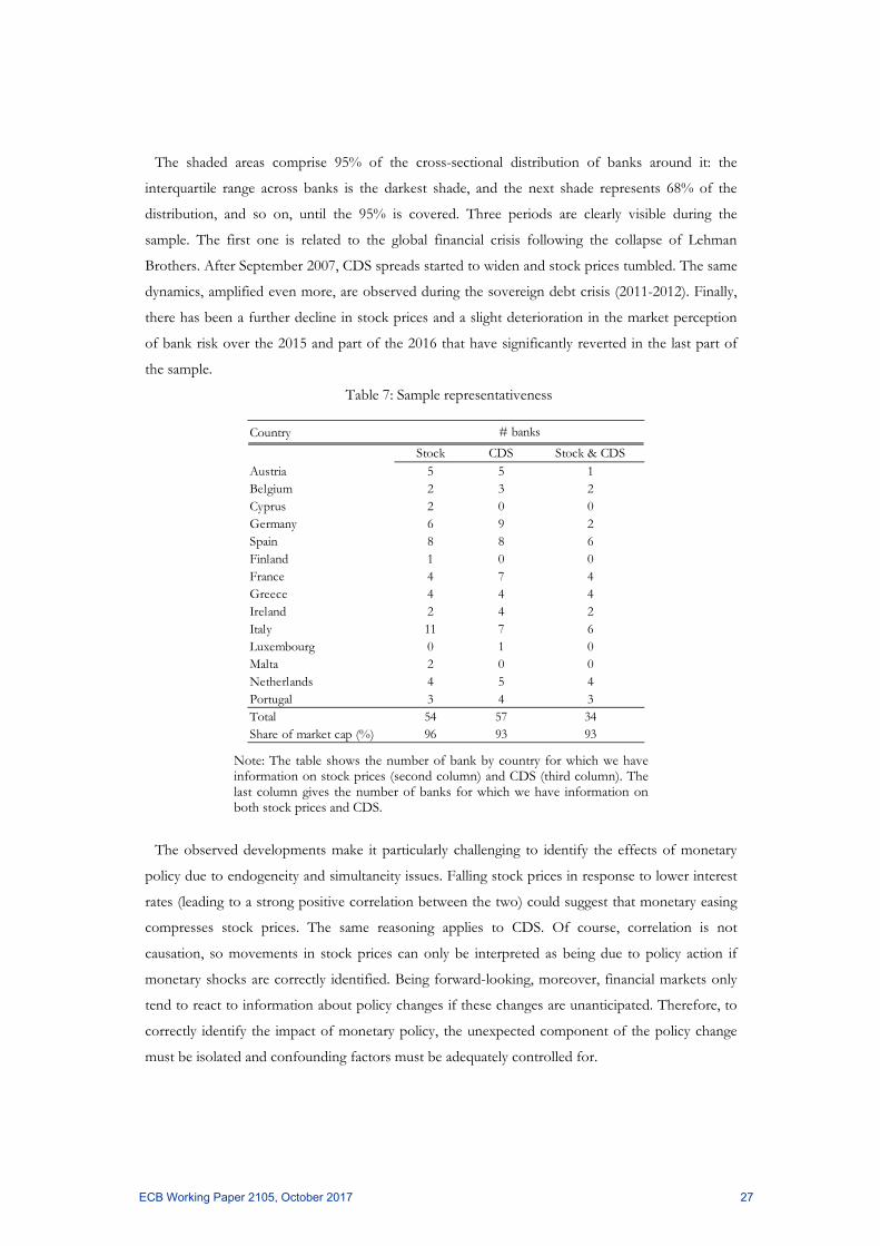
The shaded areas comprise 95% of the cross-sectional distribution of banks around it: the

interquartile range across banks is the darkest shade, and the next shade represents 68% of the

distribution, and so on, until the 95% is covered. Three periods are clearly visible during the

sample. The first one is related to the global financial crisis following the collapse of Lehman

Brothers. After September 2007, CDS spreads started to widen and stock prices tumbled. The same

dynamics, amplified even more, are observed during the sovereign debt crisis (2011-2012). Finally,

there has been a further decline in stock prices and a slight deterioration in the market perception

of bank risk over the 2015 and part of the 2016 that have significantly reverted in the last part of

the sample.

Table 7: Sample representativeness

Note: The table shows the number of bank by country for which we have information on stock prices (second column) and CDS (third column). The last column gives the number of banks for which we have information on both stock prices and CDS.

The observed developments make it particularly challenging to identify the effects of monetary

policy due to endogeneity and simultaneity issues. Falling stock prices in response to lower interest

rates (leading to a strong positive correlation between the two) could suggest that monetary easing

compresses stock prices. The same reasoning applies to CDS. Of course, correlation is not

causation, so movements in stock prices can only be interpreted as being due to policy action if

monetary shocks are correctly identified. Being forward-looking, moreover, financial markets only

tend to react to information about policy changes if these changes are unanticipated. Therefore, to

correctly identify the impact of monetary policy, the unexpected component of the policy change

must be isolated and confounding factors must be adequately controlled for.

Country

Stock CDS Stock & CDSAustria 5 5 1Belgium 2 3 2Cyprus 2 0 0Germany 6 9 2Spain 8 8 6Finland 1 0 0France 4 7 4Greece 4 4 4Ireland 2 4 2Italy 11 7 6Luxembourg 0 1 0Malta 2 0 0Netherlands 4 5 4Portugal 3 4 3Total 54 57 34Share of market cap (%) 96 93 93

# banks


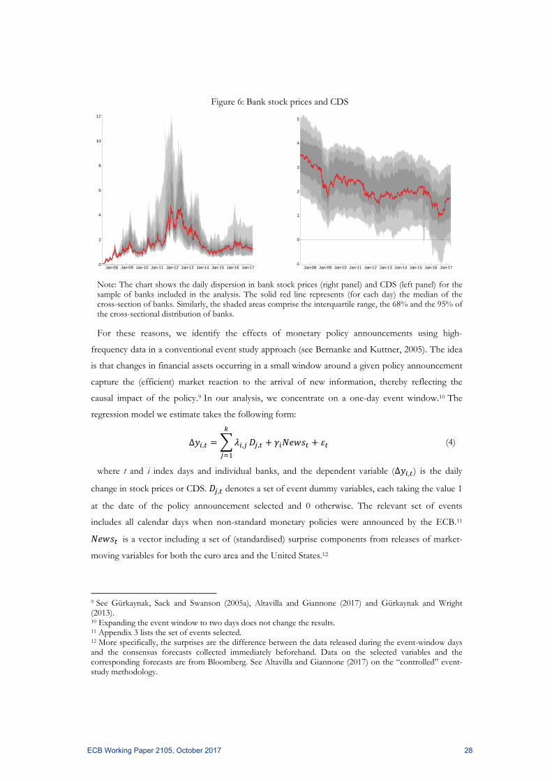
Figure 6: Bank stock prices and CDS

Note: The chart shows the daily dispersion in bank stock prices (right panel) and CDS (left panel) for the sample of banks included in the analysis. The solid red line represents (for each day) the median of the cross-section of banks. Similarly, the shaded areas comprise the interquartile range, the 68% and the 95% of the cross-sectional distribution of banks.

For these reasons, we identify the effects of monetary policy announcements using high-

frequency data in a conventional event study approach (see Bernanke and Kuttner, 2005). The idea

is that changes in financial assets occurring in a small window around a given policy announcement

capture the (efficient) market reaction to the arrival of new information, thereby reflecting the

causal impact of the policy.9 In our analysis, we concentrate on a one-day event window.10 The

regression model we estimate takes the following form:

Δ , , , (4)

where t and i index days and individual banks, and the dependent variable (Δ , ) is the daily

change in stock prices or CDS. , denotes a set of event dummy variables, each taking the value 1

at the date of the policy announcement selected and 0 otherwise. The relevant set of events

includes all calendar days when non-standard monetary policies were announced by the ECB.11

is a vector including a set of (standardised) surprise components from releases of market-

moving variables for both the euro area and the United States.12

9 See Gürkaynak, Sack and Swanson (2005a), Altavilla and Giannone (2017) and Gürkaynak and Wright (2013). 10 Expanding the event window to two days does not change the results. 11 Appendix 3 lists the set of events selected. 12 More specifically, the surprises are the difference between the data released during the event-window days and the consensus forecasts collected immediately beforehand. Data on the selected variables and the corresponding forecasts are from Bloomberg. See Altavilla and Giannone (2017) on the “controlled” event-study methodology.

Jan-08 Jan-09 Jan-10 Jan-11 Jan-12 Jan-13 Jan-14 Jan-15 Jan-16 Jan-170

2

4

6

8

10

12

Jan-08 Jan-09 Jan-10 Jan-11 Jan-12 Jan-13 Jan-14 Jan-15 Jan-16 Jan-17-1

0

1

2

3

4

5


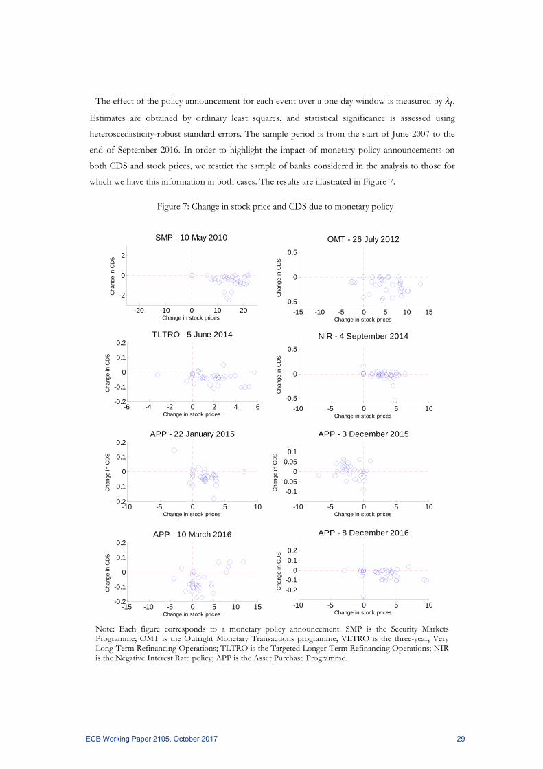
The effect of the policy announcement for each event over a one-day window is measured by .

Estimates are obtained by ordinary least squares, and statistical significance is assessed using

heteroscedasticity-robust standard errors. The sample period is from the start of June 2007 to the

end of September 2016. In order to highlight the impact of monetary policy announcements on

both CDS and stock prices, we restrict the sample of banks considered in the analysis to those for

which we have this information in both cases. The results are illustrated in Figure 7.

Figure 7: Change in stock price and CDS due to monetary policy

Note: Each figure corresponds to a monetary policy announcement. SMP is the Security Markets Programme; OMT is the Outright Monetary Transactions programme; VLTRO is the three-year, Very Long-Term Refinancing Operations; TLTRO is the Targeted Longer-Term Refinancing Operations; NIR is the Negative Interest Rate policy; APP is the Asset Purchase Programme.

-20 -10 0 10 20

-2

0

2

Change in stock prices

Cha

nge

in C

DS

SMP - 10 May 2010

-15 -10 -5 0 5 10 15

-0.5

0

0.5


Cha

nge

in C

DS

OMT - 26 July 2012

-6 -4 -2 0 2 4 6-0.2

-0.1

0

0.1

0.2


Cha

nge

in C

DS

TLTRO - 5 June 2014

-10 -5 0 5 10

-0.5

0

0.5


Cha

nge

in C

DS

NIR - 4 September 2014

-10 -5 0 5 10-0.2

-0.1

0

0.1

0.2


Cha

nge

in C

DS

APP - 22 January 2015

-10 -5 0 5 10

-0.1

-0.05

0

0.05

0.1


Cha

nge

in C

DS

APP - 3 December 2015

-15 -10 -5 0 5 10 15-0.2

-0.1

0

0.1

0.2


Cha

nge

in C

DS

APP - 10 March 2016

-10 -5 0 5 10

-0.2

-0.10

0.1

0.2


Cha

nge

in C

DS

APP - 8 December 2016


For each of the eight selected policy events and for each bank (denoted by a blue circle in the

charts), the x-axis reports the change in stock prices while the y-axis reports the change in CDS

spreads. The results are striking: for the vast majority of banks, stock prices increased and CDS

spreads narrowed following all major monetary policy announcements.

This suggests that financial market participants reacted positively to the announcement of the new

policies. The only exception is the announcement of the recalibration of the APP scheme in

December 2015, which is associated with a fall in stock prices (second-to-last chart on the right of

the figure). This is, however, easy to understand, as financial market participants interpreted the

December policy decision as delivering lower-than-expected accommodation compared with what

they had anticipated and factored into stock prices. The policy decision therefore elicited an

opposite reaction in financial markets when announced. This announcement, however, is also

characterised by a heterogeneous response of bank CDS.

In principle, there are different reasons why a monetary easing may lead to an increase in stock

prices. First, financial markets might perceive that the looser policy may generate an increase in

expected future dividends. Second, accommodative policy may be associated with a decline in the

discount rate, being the future expected real interest rates used to discount the dividends. Third, the

policy easing may compress the equity premium. In order to exclude the effect related to the

discount factor, we repeat the same exercise for stock market indices of different industries. As the

effect of the discount factor should affect all industries equally, the remaining differences should be

attributed to changes in the equity premium associated with holding stocks or to the expected

future dividends. Figure 8 shows that, although industry-based portfolios tend to react in a similar

direction, the size of the response may vary substantially.

Overall, the index for the banking sector exhibits the largest response to most of the events. For

utilities and insurance companies – which tend to be significantly less leveraged than banks – the

effect of monetary policies is more muted. These results corroborate the previous evidence on the

positive impact of non-standard measures on bank stock valuations (e.g. English et al., 2014).


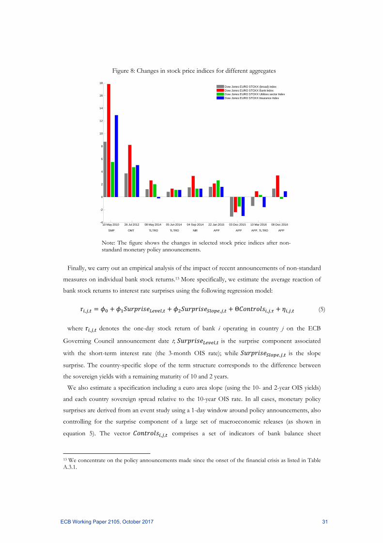
Figure 8: Changes in stock price indices for different aggregates

Note: The figure shows the changes in selected stock price indices after non-standard monetary policy announcements.

Finally, we carry out an empirical analysis of the impact of recent announcements of non-standard

measures on individual bank stock returns.13 More specifically, we estimate the average reaction of

bank stock returns to interest rate surprises using the following regression model:

r , , , , , Θ , , , , (5)

where r , , denotes the one-day stock return of bank i operating in country j on the ECB

Governing Council announcement date t; , is the surprise component associated

with the short-term interest rate (the 3-month OIS rate); while , , is the slope

surprise. The country-specific slope of the term structure corresponds to the difference between

the sovereign yields with a remaining maturity of 10 and 2 years.

We also estimate a specification including a euro area slope (using the 10- and 2-year OIS yields)

and each country sovereign spread relative to the 10-year OIS rate. In all cases, monetary policy

surprises are derived from an event study using a 1-day window around policy announcements, also

controlling for the surprise component of a large set of macroeconomic releases (as shown in

equation 5). The vector , , comprises a set of indicators of bank balance sheet

13 We concentrate on the policy announcements made since the onset of the financial crisis as listed in Table A.3.1.

10 May 2010 26 Jul 2012 08 May 2014 05 Jun 2014 04 Sep 2014 22 Jan 2015 03 Dec 2015 10 Mar 2016 08 Dec 2016-4

-2

0

2

4

6

8

10

12

14

16

18

Dow Jones EURO STOXX (broad) indexDow Jones EURO STOXX Bank IndexDow Jones EURO STOXX Utilities sector IndexDow Jones EURO STOXX Insurance Index

SMP OMT TLTRO TLTRO NIR APP APP APP, TLTRO APP


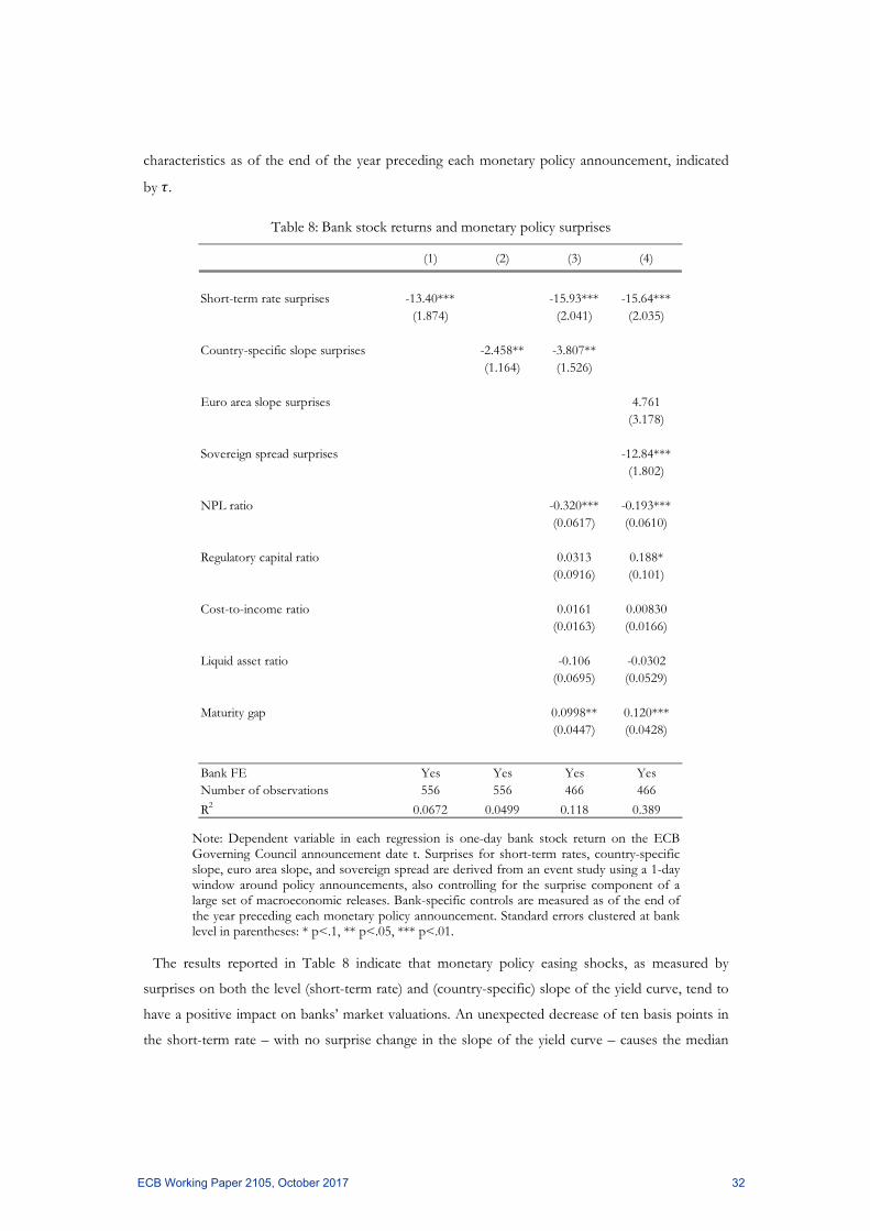
characteristics as of the end of the year preceding each monetary policy announcement, indicated

by .

Table 8: Bank stock returns and monetary policy surprises

Note: Dependent variable in each regression is one-day bank stock return on the ECB Governing Council announcement date t. Surprises for short-term rates, country-specific slope, euro area slope, and sovereign spread are derived from an event study using a 1-day window around policy announcements, also controlling for the surprise component of a large set of macroeconomic releases. Bank-specific controls are measured as of the end of the year preceding each monetary policy announcement. Standard errors clustered at bank level in parentheses: * p<.1, ** p<.05, *** p<.01.

The results reported in Table 8 indicate that monetary policy easing shocks, as measured by

surprises on both the level (short-term rate) and (country-specific) slope of the yield curve, tend to

have a positive impact on banks’ market valuations. An unexpected decrease of ten basis points in

the short-term rate – with no surprise change in the slope of the yield curve – causes the median

(1) (2) (3) (4)

Short-term rate surprises -13.40*** -15.93*** -15.64***(1.874) (2.041) (2.035)

Country-specific slope surprises -2.458** -3.807**(1.164) (1.526)

Euro area slope surprises 4.761(3.178)

Sovereign spread surprises -12.84***(1.802)

NPL ratio -0.320*** -0.193***(0.0617) (0.0610)

Regulatory capital ratio 0.0313 0.188*(0.0916) (0.101)

Cost-to-income ratio 0.0161 0.00830(0.0163) (0.0166)

Liquid asset ratio -0.106 -0.0302(0.0695) (0.0529)

Maturity gap 0.0998** 0.120***(0.0447) (0.0428)

Bank FE Yes Yes Yes YesNumber of observations 556 556 466 466

R2 0.0672 0.0499 0.118 0.389


bank’s stock price to increase by about 1.5% (column 3); a shock to the country-specific slope of

the yield curve of the same magnitude is estimated to increase the bank’s stock price by about 0.4%

(column 3).

Regarding the control variables, bank asset quality is negatively associated with bank stock return.

A 1% increase in the NPL ratio translates into a 20-30 basis point decrease in bank stock returns on

monetary policy announcement dates. Importantly, and in line with the analysis presented in the

previous sections, stock returns are higher for banks engaging more in maturity transformation. An

additional month of difference between the weighted average maturity of asset and liabilities

increases the bank stock return by 0.1%.

6 Conclusions In this paper, we have analysed the implications of alternative monetary policy actions on bank

profitability and on market-based measures of bank shareholder value and bank risk. For empirical

identification, we focus on the euro area, which provides an interesting case study as it includes

substantial bank and country heterogeneity within a monetary union where a broad set of

unconventional policies, including negative interest rates, credit and quantitative easing have been

implemented. Moreover, we exploit proprietary ECB data on individual bank balance sheets since

2007, and data from commercial providers since the creation of the euro area. We have tackled our

question by analysing different types of data – ranging from the daily frequency of the event study

to the quarterly frequency of the bank balance sheet indicators – and over different sample periods.

The results suggest some robust findings.

First, monetary policy easing, summarised as either a decrease in short-term interest rates or a

flattening of the yield curve, is only associated with lower bank profits if there are no appropriate

controls for the endogeneity of monetary policy to bank financial health – especially during the

crisis period – as well as to current and expected aggregate economic and financial conditions.

Second, policy easing tends to be more beneficial in relative terms for more efficient banks and

for banks with lower asset quality. At the same time, banks engaging more extensively in maturity

transformation activities tend to have a more positive reaction to a steepening of the yield curve.

Importantly, our analysis suggests that keeping interest rates low for long might have negative

consequences for bank profitability. However, we find that it takes a long period of time for

monetary policy to exert a substantial adverse effect on bank profitability as a result of looser

policies. Furthermore, lower interest rates in general support real economic activity which, in turn,

has a positive impact on bank profitability, thereby offsetting the adverse impact.

Third, evidence from both a panel data model that uses individual bank balance sheet data and a

dynamic multivariate model that uses more aggregate data, suggest that following a monetary policy


shock, the various components of bank profitability react asymmetrically. More specifically, since

the impact on loan loss provisions largely offsets the one on net interest income, the overall effects

of monetary policy on bank profitability are muted.

Finally, market-based expectations on future bank profitability are analysed looking at the high-

frequency changes in bank stock returns around monetary policy announcement dates. Financial

market evidence suggests that both bank debtholders and shareholders tend to be better off when

the central bank announces new, accommodative monetary policy. This is important not only for

financial stability and systemic risk but also for the possible distributional consequences that these

policies may have on bank shareholders and debtholders, including depositors.


References Admati, Anad and Hellwig, Martin (2014), The Bankers’ New Clothes: What’s Wrong with Banking and

What to Do About it, Princeton University Press, Princeton, NJ.

Albertazzi, Ugo and Gambacorta, Leonardo (2009), “Bank profitability and the business cycle”,

Journal of Financial Stability, Elsevier, Vol. 5, Issue 4, pp. 393-409.

Alessandri, Piergiorgio and Nelson, Benjamin D. (2015), “Simple Banking: Profitability and the

Yield Curve”, Journal of Money, Credit and Banking, Blackwell Publishing, Vol. 47, Issue 1, pp. 143-

175, 02.

Allen, Franklin and Rogoff, Kenneth (2011), “Asset prices, financial stability and monetary

policy”, in Jansson, P. and Persson, M. (eds.), The Riksbank’s inquiry into the risks in the Swedish housing

market, Sveriges Riksbank, Stockholm, pp. 189-218.

Allen, F., Carletti E. and Gale D. (2009), “Interbank Market Liquidity and Central Bank

Intervention”, Journal of Monetary Economics, Elsevier, Vol. 56, Issue 5, pp. 639-652.

Allen, F., Carletti E. and Gale D. (2014), “Money, Financial Stability and Efficiency”, Journal of

Economic Theory, Elsevier, Vol. 149, pp. 100-127.

Altavilla, C., Canova, F. and Ciccarelli, M. (2016), “Mending the broken link: heterogeneous bank

lending and monetary policy pass-through”, Working Paper Series, No 1978, European Central Bank.

Altavilla C., Carboni G., Motto R. (2015): Asset Purchase Programmes and Financial Markets:

evidence from the Euro Area, Working Paper Series 1864, European Central Bank

Altavilla, C. and Giannone, D. (2017), “The Effectiveness of Non-Standard Monetary Policy

Measures: Evidence from Survey Data”, Journal of Applied Econometrics, vol. 32 (5), pages 952–964.

Begenau, Juliane, Piazzesi, Monika and Schneider, Martin (2015), “Banks’ Risk Exposures”,

NBER Working Paper No 21334, National Bureau of Economic Research.

Bernanke, Ben S. (1983), “Non-Monetary Effects of the Financial Crisis in the Propagation of the

Great Depression”, The American Economic Review, Vol. 73, No 3 (June), pp. 257-276.

Bernanke, Ben S. and Blinder, Alan S. (1988), “Credit, Money, and Aggregate Demand”, The

American Economic Review, American Economic Association, Vol. 78, No 2, pp. 435-439.

Bernanke, Ben S. and Blinder, Alan S. (1992), “The Federal Funds Rate and the Channels of

Monetary Transmission”, The American Economic Review, American Economic Association, Vol. 82,

No 4, pp. 901-921.

Bernanke, Ben S. and Gertler, Mark (1995), “Inside the Black Box: The Credit Channel of

Monetary Policy Transmission”, Journal of Economic Perspectives, American Economic Association,

Vol. 9, No 4, pp. 27-48.

Bernanke, Ben S. (2007), speech at The Credit Channel of Monetary Policy in the Twenty-first

Century Conference, Federal Reserve Bank of Atlanta, Atlanta, Georgia.


Bernanke, Ben S. and Kuttner, Kenneth N. (2005), “What Explains the Stock Market’s Reaction

to Federal Reserve Policy?”, The Journal of Finance, American Finance Association, Vol. 60, No 3, pp.

1221-1257.

Bolt, Wilko, de Haan, Leo, Hoeberichts, Marco, van Oordt, Maarten R.C. and Swank, Job (2012),

“Bank profitability during recessions”, Journal of Banking & Finance, Elsevier, Vol. 36, Issue 9, pp.

2552-2564.

Borio C, Gambacorta L, Hofmann B. (2017) The influence of monetary policy on bank

profitability, International Finance, 20:48–63.

Bourke, Philip (1989), “Concentration and other determinants of bank profitability in Europe,

North America and Australia”, Journal of Banking & Finance, Elsevier, Vol. 13, Issue 1, pp. 65-79.

Brunnermeier, Markus K., and Yann Koby (2017) “The Reversal Interest Rate: The Effective

Lower Bound of Monetary Policy”, mimeo, version July 10, 2017.

Claessens, Stijn, Coleman, Nicholas and Donnelly, Michael (2017), ‘Low-For-Long’ Interest Rates

and Banks’ Interest Margins and Profitability: Cross-Country Evidence, CEPR Discussion Paper No

11842, Centre for Economic Policy Research.

De Mol, C., Giannone, D. and Reichlin, L. (2008), Forecasting using a large number of predictors:

Is Bayesian shrinkage a valid alternative to principal components?, Journal of Econometrics, Vol.

146(2), pp. 318-328.

Diamond, Doug and Rajan, Raghuram (2006), Money in a Theory of Banking, The American

Economic Review, American Economic Association, Vol. 96, No 1, pp. 30-53.

El-Erian, Mohamed A. (2016), The Only Game in Town: Central Banks, Instability, and Avoiding the

Next Collapse, Penguin Random House.

English, W.B., Van den Heuvel, S. and Zakrajsek, E. (2012), “Interest Rate Risk and Bank Equity

Valuations”, Finance and Economics Discussion Series, Board of Governors of the Federal Reserve

System, pp. 2012-2026.

Flannery, Mark J. (1981), “Market Interest Rates and Commercial Bank Profitability: An

Empirical Investigation”, Journal of Finance, American Finance Association, Vol. 36, pp. 1085-1101.

Flannery, Mark J. (1983), “Interest Rates and Bank Profitability: Additional Evidence”, Journal of

Money, Credit and Banking, Blackwell Publishing, Vol. 15, Issue 3, pp. 355-362.

Freixas, Xavier, Laeven, Luc and Peydró, José-Luis (2015), Systemic Risk, Crises, and Macroprudential

Regulation, MIT Press, Cambridge, MA.

Freixas, Xavier and Rochet Jean-Charles (2008), Microeconomics of Banking, MIT Press, Cambridge,

MA.

Freixas, Xavier and Jorge, José (2008), “The Role of Interbank Markets in Monetary Policy: A

Model with Rationing”, Journal of Money, Credit and Banking, The Ohio State University, Vol. 40, No

6, pp. 1151-1176.


Freixas, Xavier, Martin, Antoine and Skeie, David (2011), “Bank Liquidity, Interbank Markets,

and Monetary Policy”, The Review of Financial Studies, Oxford University Press, Vol. 24, Issue 8, pp.

2656-2692.

Genay, Hesna & Podjasek, Rich (2014), “What Is the Impact of a Low Interest Rate Environment

on Bank Profitability?”, Chicago Fed Letter, Federal Reserve Bank of Chicago, July.

Gertler, Mark and Kiyotaki, Nobuhiro (2010), “Financial Intermediation and Credit Policy in

Business Cycle Analysis,” in Friedman B.M. and Woodford, M. (eds.), Handbook of Monetary

Economics, Elsevier, Vol 3, pp. 547-599.

Gertler, Mark and Karadi, Peter (2011), “A Model of Unconventional Monetary Policy”, Journal of

Monetary Economics, Vol. 58, Issue 1, pp. 17-34.

Gertler, Mark and Karadi, Peter (2013), “QE 1 vs. 2 vs. 3. . . : A Framework for Analyzing Large-

Scale Asset Purchases as a Monetary Policy Tool”, International Journal of Central Banking, IJCB, Vol.

9, No 1, pp. 5-53.

Giannone, D., Lenza, M. and Primiceri, G. (2015), “Priors for Vector Autoregressions”, Review of

Economics and Statistics, Vol. 2(97), pp. 436-451.

Gürkaynak, R.S. and Wright, J.H. (2013), “Identification and Inference Using Event Studies”,

CEPR Discussion Papers No 9388, Centre for Economic Policy Research,

Gürkaynak, R.S., Sack, B. and Swanson, E. (2005a), “The Sensitivity of Long-Term Interest Rates

to Economic News: Evidence and Implications for Macroeconomic Models”, The American Economic

Review, American Economic Association, Vol. 95, No 1, pp. 425-436.

Gürkaynak, R.S., Sack, B. and Swanson, E. (2005b), “Do Actions Speak Louder Than Words?

The Response of Asset Prices to Monetary Policy Actions and Statements”, International Journal of

Central Banking, 1 (1) (2005), pp. 55-92 Hancock, Diana (1985), “Bank Profitability, Interest Rates,

and Monetary Policy”, Journal of Money, Credit and Banking, The Ohio State University, Vol. 17, pp.

189-202.

Hoffmann P., S. Langfield, F. Pierobon, G. Vuillemey (2017) Who bears interest rate risk?, mimeo

Jiménez, Gabriel, Ongena, Steven, Peydró, José-Luis and Saurina, Jesús (2012), “Credit Supply

and Monetary Policy: Identifying the Bank Balance-Sheet Channel with Loan Applications”, The


Jiménez, Gabriel, Ongena, Steven, Peydró, José-Luis and Saurina, Jesús (2014), “Hazardous Times

for Monetary Policy: What Do Twenty‐Three Million Bank Loans Say about the Effects of

Monetary Policy on Credit Risk‐Taking?”, Econometrica, The Econometric Society, Vol. 82, Issue 2,

pp. 463-505.


Jiménez, Gabriel, Ongena, Steven, Peydró, José-Luis and Saurina, Jesús (2017), “Macroprudential

Policy, Countercyclical Bank Capital Buffers and Credit Supply: Evidence from the Spanish

Dynamic Provisioning Experiments”, Journal of Political Economy, forthcoming.

Kashyap, Anil and Stein, Jeremy (2000), “What Do a Million Observations on Banks Say about

the Transmission of Monetary Policy?”, The American Economic Review, American Economic

Association, Vol. 90, No 3, pp. 407-428.

Kindleberger, Charles P. (1978), Manias, Panics, and Crashes: A History of Financial Crises, Basic

Books, New York.

Kiyotaki, N. and Moore, J. (2012), “Liquidity, Business Cycles, and Monetary Policy”, NBER

Working Paper No 17934, National Bureau of Economic Research.

Maudos, Joaquin and Fernandez de Guevara, Juan (2004), “Factors explaining the interest margin

in the banking sectors of the European Union”, Journal of Banking and Finance, Elsevier, Vol. 28,

Issue 9, pp. 2259-2281.

Nickell, S. (1981), “Biases in Dynamic Models with Fixed Effects”, Econometrica, The Econometric

Society, Vol. 49, Issue 6, pp. 1417-1426.

Praet, P. (2016), “Monetary policy and the euro area banking system”, speech by Peter Praet,

Member of the Executive Board of the ECB, Madrid, 4 October.

Rajan, Raghuram (2005), “Has finance made the world riskier?”, speech presented at Jackson

Hole, Federal Reserve Bank, Federal Reserve Bank, August.

Reinhart, Carmen M., and Rogoff, Kenneth S. (2009), “The Aftermath of Financial Crises”, The


Saunders, Anthony and Schumacher, Liliana (2000), “The Determinants of Bank Interest Rate

Margins: An International Study”, Journal of International Money & Finance, Vol. 19 (6), pp. 813-832.

Sims, C. A. (1993), “A Nine-Variable Probabilistic Macroeconomic Forecasting Model”, Business

Cycles, Indicators and Forecasting, NBER Chapters, pp. 179-212.

Stiglitz, Joseph (2016), “The Theory of Credit and Macro-economic Stability”, NBER Working

Paper No 22837, National Bureau of Economic Research.

Stein, J.C. (2012), “Monetary Policy as Financial Stability Regulation”, The Quarterly Journal of

Economics, Vol. 127, Issue 1, pp. 57-95.

Stein, J.C. (2014), “Incorporating Financial Stability Considerations into a Monetary Policy

Framework”, speech given at the International Research Forum on Monetary Policy, Washington,

D.C., 21 March, and at the International Monetary Fund 2014 Spring Meetings.

Taylor, John (2008), “The financial crisis and the policy responses: an empirical analysis of what

went wrong”, NBER Working Paper No 14631, National Bureau of Economic Research.

Thorbecke, Willem (1997), “On Stock Market Returns and Monetary Policy”, Journal of Finance,

American Finance Association, Vol. 52, Issue 2, pp. 635-654.


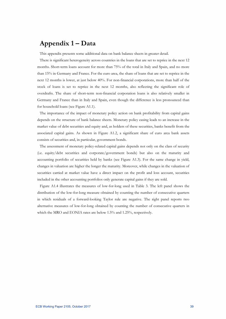
Appendix 1 – Data This appendix presents some additional data on bank balance sheets in greater detail.

There is significant heterogeneity across countries in the loans that are set to reprice in the next 12

months. Short-term loans account for more than 75% of the total in Italy and Spain, and no more

than 15% in Germany and France. For the euro area, the share of loans that are set to reprice in the

next 12 months is lower, at just below 40%. For non-financial corporations, more than half of the

stock of loans is set to reprice in the next 12 months, also reflecting the significant role of

overdrafts. The share of short-term non-financial corporation loans is also relatively smaller in

Germany and France than in Italy and Spain, even though the difference is less pronounced than

for household loans (see Figure A1.1).

The importance of the impact of monetary policy action on bank profitability from capital gains

depends on the structure of bank balance sheets. Monetary policy easing leads to an increase in the

market value of debt securities and equity and, as holders of these securities, banks benefit from the

associated capital gains. As shown in Figure A1.2, a significant share of euro area bank assets

consists of securities and, in particular, government bonds.

The assessment of monetary policy-related capital gains depends not only on the class of security

(i.e. equity/debt securities and corporate/government bonds) but also on the maturity and

accounting portfolio of securities held by banks (see Figure A1.3). For the same change in yield,

changes in valuation are higher the longer the maturity. Moreover, while changes in the valuation of

securities carried at market value have a direct impact on the profit and loss account, securities

included in the other accounting portfolios only generate capital gains if they are sold.

Figure A1.4 illustrates the measures of low-for-long used in Table 3. The left panel shows the

distribution of the low-for-long measure obtained by counting the number of consecutive quarters

in which residuals of a forward-looking Taylor rule are negative. The right panel reports two

alternative measures of low-for-long obtained by counting the number of consecutive quarters in

which the MRO and EONIA rates are below 1.5% and 1.25%, respectively.


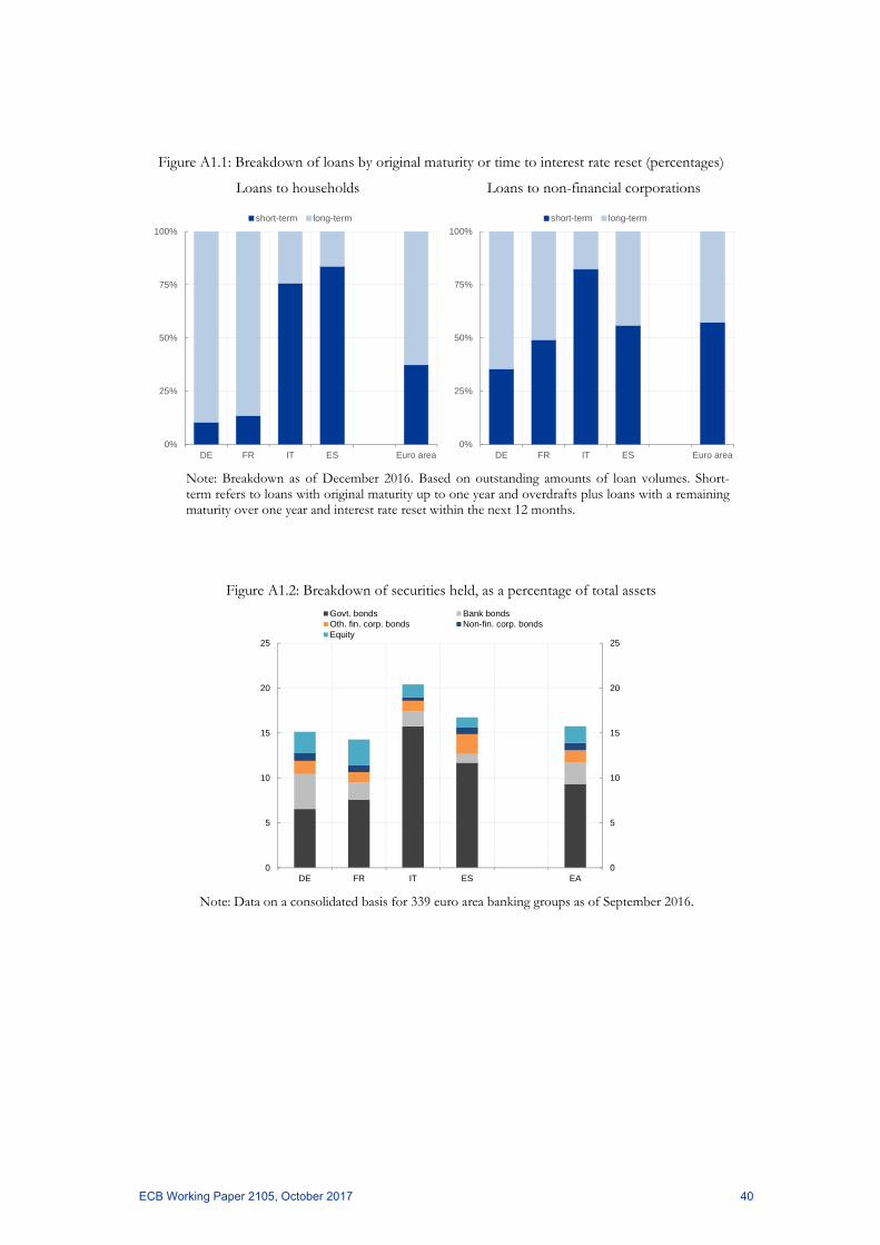
Figure A1.1: Breakdown of loans by original maturity or time to interest rate reset (percentages)

Loans to households Loans to non-financial corporations

Note: Breakdown as of December 2016. Based on outstanding amounts of loan volumes. Short-term refers to loans with original maturity up to one year and overdrafts plus loans with a remaining maturity over one year and interest rate reset within the next 12 months.

Figure A1.2: Breakdown of securities held, as a percentage of total assets

Note: Data on a consolidated basis for 339 euro area banking groups as of September 2016.

0%

25%

50%

75%

100%

DE FR IT ES Euro area

short-term long-term

0%

25%

50%

75%

100%

DE FR IT ES Euro area

short-term long-term

0

5

10

15

20

25

0

5

10

15

20

25

DE FR IT ES EA

Govt. bonds Bank bondsOth. fin. corp. bonds Non-fin. corp. bondsEquity


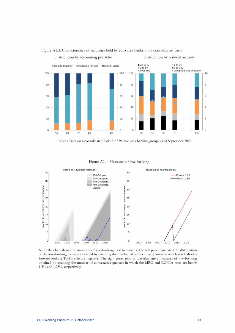
Figure A1.3: Characteristics of securities held by euro area banks, on a consolidated basis

Distribution by accounting portfolio Distribution by residual maturity

Notes: Data on a consolidated basis for 339 euro area banking groups as of September 2016.

Figure A1.4: Measures of low for long

Note: the chart shows the measures of low-for-long used in Table 3. The left panel illustrated the distribution of the low-for-long measure obtained by counting the number of consecutive quarters in which residuals of a forward-looking Taylor rule are negative. The right panel reports two alternative measures of low-for-long obtained by counting the number of consecutive quarters in which the MRO and EONIA rates are below 1.5% and 1.25%, respectively.

0

20

40

60

80

100

0

20

40

60

80

100

DE FR IT ES EA

Held to maturity Available for sale Market value

0

2

4

6

8

10

0

20

40

60

80

100

DE ES FR IT EA

up to 1y 1 to 2y2 to 5y 5 to 10yover 10y Weighted avg. maturity

2002 2005 2007 2010 2012 20150

5

10

15

20

25

30

35

40

mo

nth

s in

low

inte

rest

ra

te e

nvi

ron

me

nt

based on Taylor rule residuals

2002 2005 2007 2010 2012 20150

5

10

15

20

25

30

35

40

mo

nth

s in

low

inte

rest

ra

te e

nvi

ron

me

nt

based on ad-hoc thresholds

95th-5th perc.90th-10th perc.84th-16th perc.75th-25th perc.Median

Eonia < 1.25MRO < 1.5%


Appendix 2 – Robustness This appendix presents additional analysis carried out to check the robustness of the results

presented in the main part of the paper.

Tables A2.1 and A2.2 replicate the results reported in Table 2 and Table 6, respectively,

constraining the sample used in the estimation to be constant across all specifications. The results

show that differences in the estimates across specifications are indeed driven by the additional

information included in the model via controls variables and not by differences in the number of

observations, which reflects differences in data availability across variables.

Table A2.3 shows that the results in Table 6 are robust to the use of the sample of banks defined

in Table 2.

In the analysis presented in the main text, the slope of the yield curve is obtained by using the

country-specific sovereign yield curve:, a bank faces a different yield curve constellation depending

on the country where it operates. In order to test whether the results change when all the banks

face a similar yield curve, we derive the slope of the term structure from the OIS rates (Table A2.4).

Specifically, in order to test whether it is indeed the euro area yield curve that matters for bank

profitability, we compare the results obtained from the baseline specification (column 1 in Table

A2.4) with those obtained using the slope derived from the OIS curve (column 2, denoted with

“euro area slope”). The coefficient is not significant. Finally, we check the importance of the

sovereign spread (column 3) and find a negative and statistically significant coefficient: a reduction

in the difference between the sovereign yields and the OIS rate at 10-year maturity is associated

with an increase in profitability.

In addition, we show below that the results reported in the paper are robust to the omission of

the fixed effects (Table A2.5) and to GMM estimation (Table A2.6).

Finally, Table A2.7 replicates the analysis on the profitability components reported in Table 4 for

the shorter sample. Comparing the two tables indicates that when focusing on a shorter sample

period the results obtained in the main text of the paper remain unchanged.


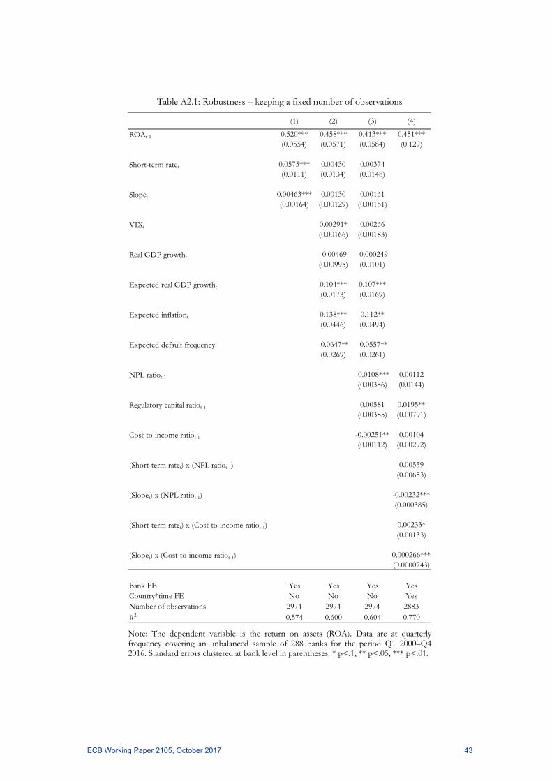
Table A2.1: Robustness – keeping a fixed number of observations


(1) (2) (3) (4)

ROAt-1 0.520*** 0.458*** 0.413*** 0.451***(0.0554) (0.0571) (0.0584) (0.129)

Short-term ratet 0.0575*** 0.00430 0.00374(0.0111) (0.0134) (0.0148)

Slopet 0.00463*** 0.00130 0.00161(0.00164) (0.00129) (0.00151)

VIXt 0.00291* 0.00266(0.00166) (0.00183)

Real GDP growtht -0.00469 -0.000249(0.00995) (0.0101)



Expected default frequencyt -0.0647** -0.0557**(0.0269) (0.0261)

NPL ratiot-1 -0.0108*** 0.00112(0.00356) (0.0144)

Regulatory capital ratiot-1 0.00581 0.0195**(0.00385) (0.00791)

Cost-to-income ratiot-1 -0.00251** 0.00104(0.00112) (0.00292)

(Short-term ratet) x (NPL ratiot-1) 0.00559(0.00653)


(Short-term ratet) x (Cost-to-income ratiot-1) 0.00233*(0.00133)


Bank FE Yes Yes Yes YesCountry*time FE No No No YesNumber of observations 2974 2974 2974 2883

R2 0.574 0.600 0.604 0.770


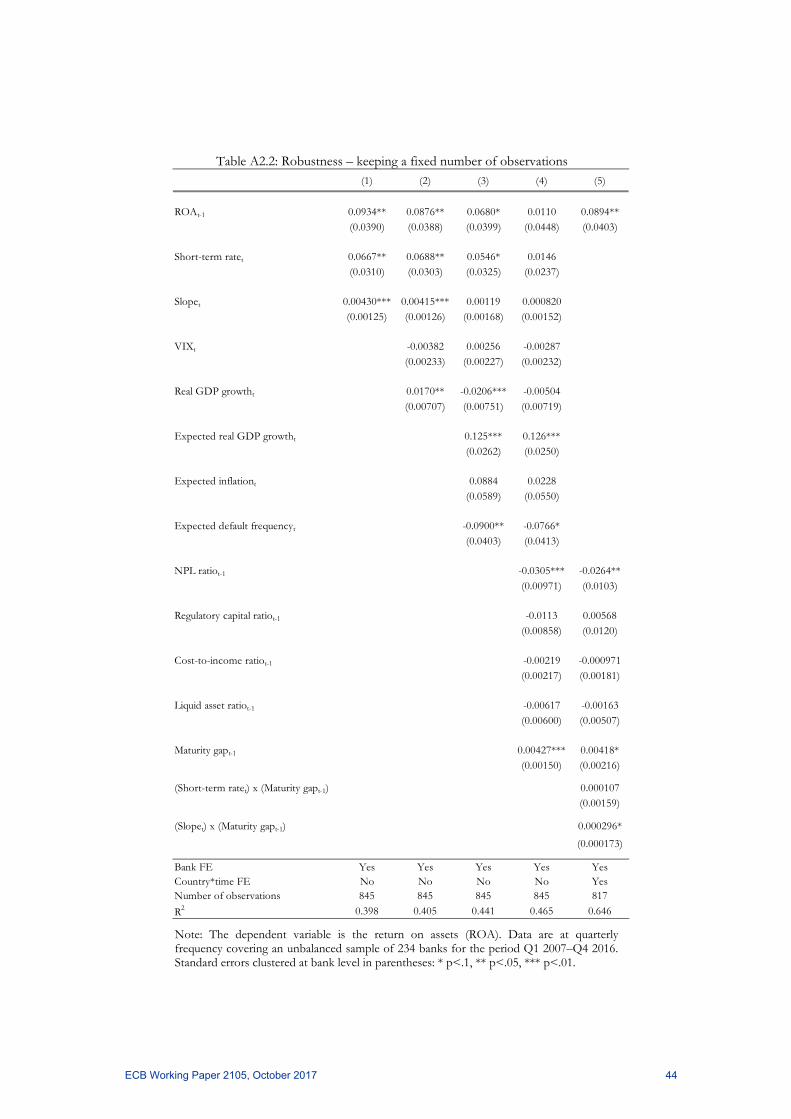
Table A2.2: Robustness – keeping a fixed number of observations


(1) (2) (3) (4) (5)

ROAt-1 0.0934** 0.0876** 0.0680* 0.0110 0.0894**(0.0390) (0.0388) (0.0399) (0.0448) (0.0403)

Short-term ratet 0.0667** 0.0688** 0.0546* 0.0146(0.0310) (0.0303) (0.0325) (0.0237)

Slopet 0.00430*** 0.00415*** 0.00119 0.000820(0.00125) (0.00126) (0.00168) (0.00152)

VIXt -0.00382 0.00256 -0.00287(0.00233) (0.00227) (0.00232)

Real GDP growtht 0.0170** -0.0206*** -0.00504(0.00707) (0.00751) (0.00719)


Expected inflationt 0.0884 0.0228(0.0589) (0.0550)

Expected default frequencyt -0.0900** -0.0766*(0.0403) (0.0413)

NPL ratiot-1 -0.0305*** -0.0264**(0.00971) (0.0103)

Regulatory capital ratiot-1 -0.0113 0.00568(0.00858) (0.0120)

Cost-to-income ratiot-1 -0.00219 -0.000971(0.00217) (0.00181)

Liquid asset ratiot-1 -0.00617 -0.00163(0.00600) (0.00507)

Maturity gapt-1 0.00427*** 0.00418*(0.00150) (0.00216)

(Short-term ratet) x (Maturity gapt-1) 0.000107(0.00159)

(Slopet) x (Maturity gapt-1) 0.000296*

(0.000173)

Bank FE Yes Yes Yes Yes YesCountry*time FE No No No No YesNumber of observations 845 845 845 845 817

R2 0.398 0.405 0.441 0.465 0.646


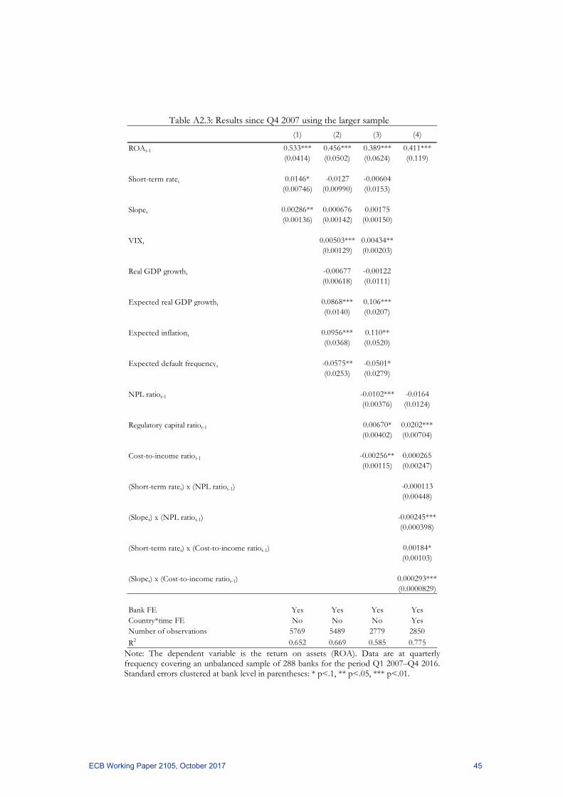
Table A2.3: Results since Q4 2007 using the larger sample


(1) (2) (3) (4)

ROAt-1 0.533*** 0.456*** 0.389*** 0.411***(0.0414) (0.0502) (0.0624) (0.119)

Short-term ratet 0.0146* -0.0127 -0.00604(0.00746) (0.00990) (0.0153)

Slopet 0.00286** 0.000676 0.00175(0.00136) (0.00142) (0.00150)

VIXt 0.00503*** 0.00434**(0.00129) (0.00203)

Real GDP growtht -0.00677 -0.00122(0.00618) (0.0111)



Expected default frequencyt -0.0575** -0.0501*(0.0253) (0.0279)

NPL ratiot-1 -0.0102*** -0.0164(0.00376) (0.0124)

Regulatory capital ratiot-1 0.00670* 0.0202***(0.00402) (0.00704)

Cost-to-income ratiot-1 -0.00256** 0.000265(0.00115) (0.00247)

(Short-term ratet) x (NPL ratiot-1) -0.000113(0.00448)


(Short-term ratet) x (Cost-to-income ratiot-1) 0.00184*(0.00103)


Bank FE Yes Yes Yes YesCountry*time FE No No No YesNumber of observations 5769 5489 2779 2850

R2 0.652 0.669 0.585 0.775


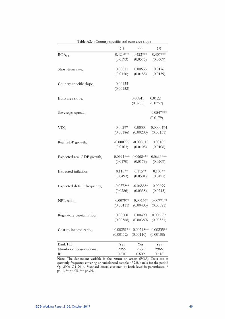
Table A2.4: Country-specific and euro area slope


(1) (2) (3)

ROAt-1 0.420*** 0.423*** 0.407***(0.0593) (0.0575) (0.0609)

Short-term ratet 0.00811 0.00655 0.0176(0.0150) (0.0158) (0.0139)

Country-specific slopet 0.00135(0.00152)

Euro area slopet 0.00841 0.0122(0.0258) (0.0257)

Sovereign spreadt -0.0547***(0.0179)

VIXt 0.00297 0.00304 0.0000494(0.00186) (0.00200) (0.00151)

Real GDP growtht -0.000777 -0.000615 0.00185(0.0103) (0.0108) (0.0106)

Expected real GDP growtht 0.0991*** 0.0968*** 0.0666***(0.0170) (0.0179) (0.0209)

Expected inflationt 0.110** 0.115** 0.108**(0.0493) (0.0501) (0.0427)

Expected default frequencyt -0.0572** -0.0688** 0.00699(0.0286) (0.0338) (0.0215)

NPL ratiot-1 -0.00797* -0.00756* -0.00771**(0.00411) (0.00403) (0.00381)

Regulatory capital ratiot-1 0.00500 0.00490 0.00668*(0.00368) (0.00380) (0.00351)

Cost-to-income ratiot-1 -0.00251** -0.00248** -0.00235**(0.00112) (0.00110) (0.00108)

Bank FE Yes Yes YesNumber of observations 2966 2966 2966R2 0.610 0.609 0.616


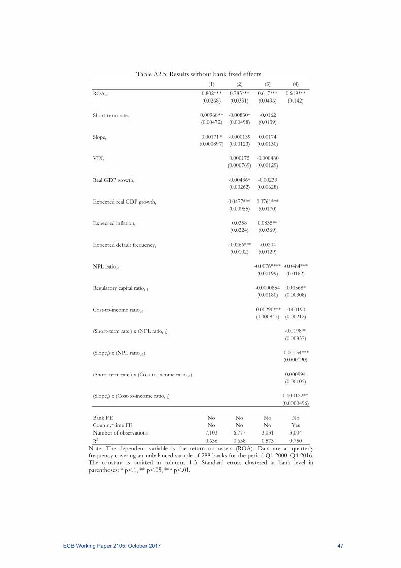
Table A2.5: Results without bank fixed effects

Note: The dependent variable is the return on assets (ROA). Data are at quarterly frequency covering an unbalanced sample of 288 banks for the period Q1 2000–Q4 2016. The constant is omitted in columns 1-3. Standard errors clustered at bank level in parentheses: * p<.1, ** p<.05, *** p<.01.

(1) (2) (3) (4)

ROAt-1 0.802*** 0.785*** 0.617*** 0.619***(0.0268) (0.0331) (0.0496) (0.142)

Short-term ratet 0.00968** -0.00830* -0.0162(0.00472) (0.00498) (0.0139)

Slopet 0.00171* -0.000139 0.00174(0.000897) (0.00123) (0.00130)

VIXt 0.000175 -0.000480(0.000769) (0.00129)

Real GDP growtht -0.00436* -0.00233(0.00262) (0.00628)


Expected inflationt 0.0358 0.0835**(0.0224) (0.0369)

Expected default frequencyt -0.0266*** -0.0204(0.0102) (0.0129)

NPL ratiot-1 -0.00765*** -0.0484***(0.00199) (0.0162)

Regulatory capital ratiot-1 -0.0000854 0.00568*(0.00180) (0.00308)

Cost-to-income ratiot-1 -0.00290*** -0.00190(0.000847) (0.00212)

(Short-term ratet) x (NPL ratiot-1) -0.0198**(0.00837)


(Short-term ratet) x (Cost-to-income ratiot-1) 0.000994(0.00105)

(Slopet) x (Cost-to-income ratiot-1) 0.000122**(0.0000496)

Bank FE No No No NoCountry*time FE No No No YesNumber of observations 7,103 6,777 3,031 3,004

R2 0.636 0.638 0.573 0.750


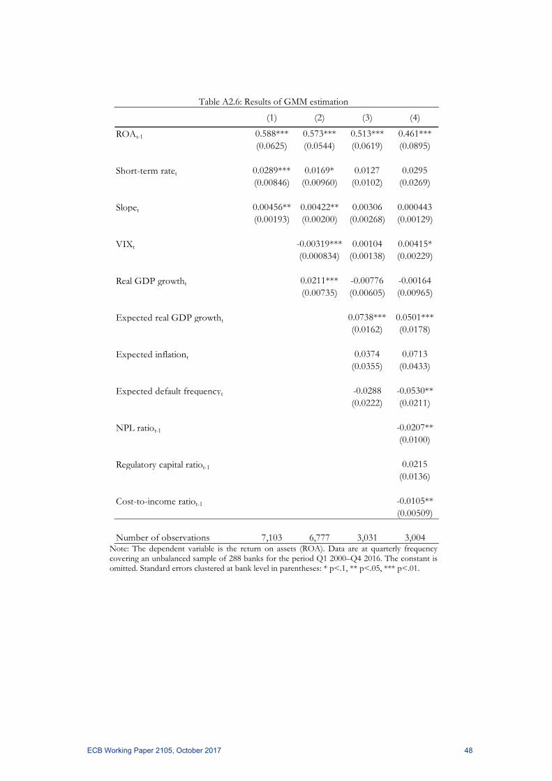
Table A2.6: Results of GMM estimation

Note: The dependent variable is the return on assets (ROA). Data are at quarterly frequency covering an unbalanced sample of 288 banks for the period Q1 2000–Q4 2016. The constant is omitted. Standard errors clustered at bank level in parentheses: * p<.1, ** p<.05, *** p<.01.

(1) (2) (3) (4)

ROAt-1 0.588*** 0.573*** 0.513*** 0.461***(0.0625) (0.0544) (0.0619) (0.0895)

Short-term ratet 0.0289*** 0.0169* 0.0127 0.0295(0.00846) (0.00960) (0.0102) (0.0269)

Slopet 0.00456** 0.00422** 0.00306 0.000443(0.00193) (0.00200) (0.00268) (0.00129)

VIXt -0.00319*** 0.00104 0.00415*(0.000834) (0.00138) (0.00229)

Real GDP growtht 0.0211*** -0.00776 -0.00164(0.00735) (0.00605) (0.00965)


Expected inflationt 0.0374 0.0713(0.0355) (0.0433)

Expected default frequencyt -0.0288 -0.0530**(0.0222) (0.0211)

NPL ratiot-1 -0.0207**(0.0100)

Regulatory capital ratiot-1 0.0215(0.0136)

Cost-to-income ratiot-1 -0.0105**(0.00509)

Number of observations 7,103 6,777 3,031 3,004


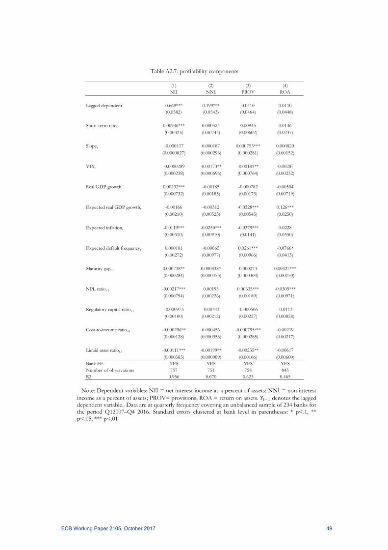
Table A2.7: profitability components

Note: Dependent variables: NII = net interest income as a percent of assets; NNI = non-interest income as a percent of assets; PROV= provisions; ROA = return on assets. denotes the lagged dependent variable.. Data are at quarterly frequency covering an unbalanced sample of 234 banks for the period Q12007–Q4 2016. Standard errors clustered at bank level in parentheses: * p<.1, ** p<.05, *** p<.01

(1) (2) (3) (4)NII NNI PROV ROA

Lagged dependent 0.669*** 0.199*** 0.0410 0.0110(0.0582) (0.0543) (0.0464) (0.0448)

Short-term ratet 0.00946*** 0.000524 0.00945 0.0146(0.00323) (0.00744) (0.00602) (0.0237)

Slopet -0.000117 0.000187 0.000753*** 0.000820(0.0000827) (0.000296) (0.000281) (0.00152)

VIXt -0.0000289 -0.00173** -0.00181** -0.00287(0.000238) (0.000696) (0.000764) (0.00232)

Real GDP growtht 0.00232*** -0.00185 -0.000782 -0.00504(0.000732) (0.00185) (0.00173) (0.00719)

Expected real GDP growtht -0.00166 -0.00312 -0.0328*** 0.126***(0.00210) (0.00523) (0.00545) (0.0250)

Expected inflationt -0.0119*** -0.0250*** -0.0379*** 0.0228(0.00310) (0.00910) (0.0141) (0.0550)

Expected default frequencyt 0.000181 -0.00865 0.0261*** -0.0766*(0.00272) (0.00977) (0.00966) (0.0413)

Maturity gapt-1 0.000738** 0.000838* 0.000273 0.00427***(0.000284) (0.000453) (0.000304) (0.00150)

NPL ratiot-1 -0.00217*** 0.00193 0.00635*** -0.0305***(0.000794) (0.00226) (0.00189) (0.00971)

Regulatory capital ratiot-1 -0.000973 -0.00343 -0.000506 -0.0113(0.00100) (0.00212) (0.00227) (0.00858)

Cost-to-income ratiot-1 -0.000296** 0.000456 -0.000795*** -0.00219(0.000128) (0.000353) (0.000285) (0.00217)

Liquid asset ratiot-1 -0.00111*** -0.00199** -0.00235** -0.00617(0.000383) (0.000989) (0.00106) (0.00600)

Bank FE YES YES YES YESNumber of observations 757 751 758 845R2 0.956 0.670 0.623 0.465


Appendix 3 – Non-standard measures

Since the onset of the financial crisis, the European Central Bank has reacted by announcing and

implementing a series of non-standard monetary policy measures. The table below presents the

main announcements used in the analysis.

Table A.3.1 Non-standard monetary policies

Note: CBPP=Covered Bond Purchase Programme; OMT=Outright Monetary Transactions programme; TLTRO=Targeted Longer-Term Refinancing Operations; NIR=Negative Interest Rate policy; APP=Asset Purchase Programme. CSPP= Corporate Sector Purchase Programme.

Date Type Announcement26/07/2012 OMT “Whatever it takes” speech by ECB President Mario Draghi in London02/08/2012 OMT Outright Monetary Transactions programme (OMT)06/09/2012 OMT Technical features of OMT

08/05/2014 TLTROPresident of the ECB explicitly stated during the press conference that the Governing Council was willing to act in the following month

05/06/2014 TLTRO, NIRTargeted longer-term refinancing operations (TLTROs); DFR=-10bps (10bps cut)

03/07/2014 TLTRO Announcement of TLTROs 04/09/2014 ABSPP , CBPP3 , NIR, APP Announcement of ABSPP, CBPP3; DFR=-20bps (10bps cut)

22/01/2015 APP

Announcement of APP1 (combined monthly purchases of €60 billion (CBPP, ABSPP, PSPP). Intended purchases: €1.14 trillion (The Governing Council also decided to modify the interest rate applicable to future TLTRO eliminating the 10bps spread over the MRO)

05/03/2015 APP APP details09/03/2015 APP APP first operation

03/12/2015 APP, NIRAPP extended until March 2017, reinvestment of principal payments, inclusion of debt instruments issued by regional and local governments; DFR=-30bps (10bps cut, MRO and MLF unchanged)

04/12/2015 APP speechSpeech by ECB President Mario Draghi, Economic Club of New York, 4 December 2015

10/03/2016 APP, TLTRO, CSPP, NIRAPP (monthly purchases expanded to €80 billion), TLTRO2, CBPSPP investment-grade euro-denominated bonds issued by non-bank corporations); DFR=-40bps (10bps cut)

08/12/2016 APP APP extended until December 2017; €60bn, DFR floor constraint dropped


Acknowledgements We would like to thank Miguel Ampudia, Philippe Andrade, Sarah Holton, Yann Koby, Benoit Mojon, Peter Praet, Elena Rancoita, Enrico Sette, Frank Smets, Andrea Tiseno, Skander Van den Heuvel and seminar participants at the ECB, Oesterreichische Nationalbank and Banque de France for their helpful comments and suggestions. The opinions in this paper are those of the authors and do not necessarily reflect the views of the European Central Bank or the Eurosystem. José-Luis Peydró acknowledges financial support from the Spanish Ministry of Economy, Industry and Competitiveness, Grant ECO2015-68136-P and FEDER, UE, and from the European Research Council Grant (project 648398). Carlo Altavilla European Central Bank, Frankfurt am Main, Germany; email: [email protected] Miguel Boucinha European Central Bank, Frankfurt am Main, Germany; email: [email protected] José-Luis Peydró ICREA-UPF, CREI, BGSE; email: [email protected]

© European Central Bank, 2017

Postal address 60640 Frankfurt am Main, Germany Telephone +49 69 1344 0 Website www.ecb.europa.eu

All rights reserved. Any reproduction, publication and reprint in the form of a different publication, whether printed or produced electronically, in whole or in part, is permitted only with the explicit written authorisation of the ECB or the authors.

This paper can be downloaded without charge from www.ecb.europa.eu, from the Social Science Research Network electronic library or from RePEc: Research Papers in Economics. Information on all of the papers published in the ECB Working Paper Series can be found on the ECB’s website.

ISSN 1725-2806 (pdf) DOI 10.2866/825393 (pdf) ISBN 978-92-899-2827-4 (pdf) EU catalogue No QB-AR-17-117-EN-N (pdf)

mailto:[email protected]



http://www.ecb.europa.eu/

http://www.ecb.europa.eu/

http://ssrn.com/

https://ideas.repec.org/s/ecb/ecbwps.html

http://www.ecb.europa.eu/pub/research/working-papers/html/index.en.html

Documents

Working Paper Series - European Central Bank · Working Paper Series . Monetary policy and bank profitability in a low interest rate environment . Carlo Altavilla , Miguel Boucinha,