Embed Size (px)
Citation preview

WORKING PAPER SERIESNO 1476 / SEPTEMBER 2012
AGING AND PENSION REFORM
EXTENDING THE RETIREMENT AGE AND HUMAN CAPITAL FORMATION
Edgar Vogel, Alexander Ludwig and Axel Börsch-Supan
NOTE: This Working Paper should not be reported as representing the views of the European Central Bank (ECB). The views expressed are
those of the authors and do not necessarily reflect those of the ECB.

© European Central Bank, 2012
AddressKaiserstrasse 29, 60311 Frankfurt am Main, Germany
Postal addressPostfach 16 03 19, 60066 Frankfurt am Main, Germany
Telephone+49 69 1344 0
Internethttp://www.ecb.europa.eu
Fax+49 69 1344 6000
All rights reserved.
ISSN 1725-2806 (online)
Any reproduction, publication and reprint in the form of a different publication, whether printed or produced electronically, in whole or in part, is permitted only with the explicit written authorisation of the ECB or the authors.
This paper can be downloaded without charge from http://www.ecb.europa.eu or from the Social Science Research Network electronic library at http://ssrn.com/abstract_id=2148393.
Information on all of the papers published in the ECB Working Paper Series can be found on the ECB’s website, http://www.ecb.europa.eu/pub/scientific/wps/date/html/index.en.html
AcknowledgementsThis research was supported by the U.S. Social Security Administration through grant # 5RRC08098400-03-00 to the National Bureau of Economic Research (NBER) as part of the SSA Retirement Research Consortium. The findings and conclusions expressed are solely those of the authors and do not represent the views of the SSA, any agency of the Federal Government, the NBER, or of the European Central Bank (ECB). Further financial support by the State of Baden-W¨urttemberg and the German Insurers Association (GDV) is gratefully acknowledged.
Edgar Vogel (corresponding author)at European Central Bank, Kaiserstrasse 29, D-60311 Frankfurt am Main, Germany; e-mail: [email protected]
Alexander Ludwig at CMR, Department of Economics and Social Sciences, University of Cologne, Albertus-Magnus-Platz, 50923 Cologne, Germany; e-mail: [email protected]
Axel Börsch-Supanat Max Planck Institute for Social Law and Social Policy, Munich Center for the Economics of Aging, Amalienstrasse 33, 80799 Mu-nich, Germany; e-mail: boersch-supan@mea mpisoc mpg.de

Abstract
Projected demographic changes in industrialized countries will reduce the share of the working-agepopulation. Analyses based on standard OLG models predict that these changes will increase the capital-labor ratio. Hence, rates of return to capital decrease and wages increase with adverse welfare conse-quences for current middle aged asset rich agents. This paper addresses three important adjustmentschannels to dampen these detrimental effects of demographic change: investing abroad, endogenous hu-man capital formation and increasing the retirement age. Our quantitative finding is that openness has arelatively mild effect. In contrast, endogenous human capital formation in combination with an increasein the retirement age has strong effects. Under these adjustments maximum welfare losses of demo-graphic change for households alive in 2010 are reduced by about 3 percentage points.
JEL classification: C68, E17, E25, J11, J24Keywords: population aging; human capital; welfare; pension reform; retirement age; open economy
1
Nontechnical Summary
The world will experience major changes in its demographic structure in the next decades. In all
countries, this process is driven by increasing life expectancy and a decline in birth rates. In
consequence, the fraction of the population in working-age will decrease and the fraction of
people in old-age will increase. This process is already well under way in industrial countries.
Standard economic analyses predict that these demographic processes will increase the capital-
labor ratio. Hence, rates of return to capital decrease and wages increase, which has adverse
welfare consequences for current cohorts who will be retired when the rate of return on assets is
low.
The purpose of this paper is to ask how strongly three channels of adjustment to these ongoing
developments and their interactions dampen such adverse welfare effects. First, compared to
industrialized countries, developing countries are relatively young. In autarky, rates of return to
capital in these economies are therefore higher. From the perspective of industrialized countries,
investing capital abroad may therefore stabilize the return to capital. Second, as raw labor will
become a relatively scarce factor and as life expectancy increases, strong incentives to invest in
human capital emanate. Such endogenous human capital adjustments may thereby substantially
mitigate the effects of aging on macroeconomic aggregates and individual welfare. Third, while
human capital adjustment increases the quality of the factor labor, a pension reform through
increasing the retirement age will increase the quantity of labor. This will increase per capita
productivity further. In addition to this direct effect, increasing the retirement age will also extend
the worklife planning horizon of households. This amplifies the incentives to accumulate human
capital.
We quantitatively evaluate these adjustment channels by developing an Auerbach and Kotlikoff
(1987) overlapping generations (OLG) model with a realistic demographic transition, two
integrated world regions, endogenous labor supply decisions and endogenous human capital
formation. As the central part of our analysis we work out the quantitative differences between a
benchmark model - with open economies and endogenous human capital formation - and counter-
factual models where industrialized countries operate in a closed economy and where human
capital may be exogenous. Along this line we emphasize the role of pension policy. We combine
2

our pension reform of increasing the retirement age with two pension scenarios of a stylized Pay-
As-You-Go pension system. In these scenarios either the contribution rate is held constant such
that - given a balanced budget and the demography - benefits are reduced or vice versa.
Our main findings about the general equilibrium feedback effects of aging - concentrating on our
constant contribution rate pension scenario – can be summarized as follows. First, newborn
agents gain from increasing wages and decreasing returns. These welfare gains are between 0.8%
and 1.1% of lifetime utility. Middle-aged and asset rich households experience losses between
6.5% and 3.6%. The size of this range strongly depends on the adjustment of human capital and
the retirement age. These losses must be compared with strong welfare gains for all future
generations. Second, while openness to international capital markets affects our predictions for
per capita GDP and other macroeconomic aggregates, the impact of openness on rates of return to
physical capital and wages is relatively small. Consequently, welfare of generations that live
through the demographic transition is relatively little affected by the degree of capital market
openness. Third, endogenous human capital formation has strong welfare effects. In the open
economy, maximum welfare losses of middle-aged households shrink from 6.5% to 4.4% when
human capital can endogenously adjust. Fourth, increasing the retirement age has similarly strong
welfare effects: maximum welfare losses of middle-aged households further shrink from 4.4% to
3.6% when the retirement age is increased. We also document that changes in retirement
legislation lead to very small feedback effects at the intensive margin. We therefore conclude
that increasing the retirement age is a very effective reform. As we will explain in more detail in
the text, the qualitative finding — that endogenous human capital is an important adjustment
mechanism — holds also in a world where we keep benefits constant and increase contributions.
However, as this would push up contribution rates the potentially welfare improving effect of
human capital is significantly dampened.
3

1 Introduction
The world will experience major changes in its demographic structure in the next decades. In all
countries, this process is mainly driven by increasing life expectancy and a decline in birth rates.
In consequence, the fraction of the population in working-age will decrease and the fraction of
people in old-age will increase. This process is already well under way in industrial countries.
Standard economic analyses predict that these demographic processes will increase the capital-
labor ratio. Hence, rates of return to capital decrease and wages increase, which has adverse
welfare consequences for current cohorts who will be retired when the rate of return on assets
is low.
The purpose of this paper is to ask how strongly three channels of adjustment to these on-
going developments and their interactions dampen such adverse welfare effects. First, com-
pared to industrialized countries, developing countries are relatively young. In autarky, rates
of return to capital in these economies are therefore higher. From the perspective of industri-
alized countries, globalization and investing capital abroad may therefore stabilize the return
to capital. Second, as raw labor will become a relatively scarce factor and as life expectancy
increases, strong incentives to invest in human capital emanate. This improves productivity.
Such endogenous human capital adjustments may thereby substantially mitigate the effects of
demographic change on macroeconomic aggregates and individual welfare. Third, while human
capital adjustment increases the quality of the factor labor, a parametric pension reform through
increasing the retirement age will increase the quantity of labor. This will increase per capita
productivity further. In addition to this direct effect, increasing the retirement age will also ex-
tend the worklife planning horizon of households. This amplifies the incentives to accumulate
human capital.
4

Point of departure of our analysis is the demographic evolution in two world regions, the
major industrial countries and the rest of the world. The left panel of figure 1 illustrates the
impact of demographic change on the working-age population ratio — the ratio of the working-
age population (of age 16− 64) to the total adult population (of age 16− 90) — and the right
panel the old-age dependency ratio — the ratio of the old population of age 65− 90 to the
working age population — in these regions. As the figure shows, the demographic structure is
subject to significant changes over time in developed and developing countries. There are large
level differences between these two regions but overall demographic trends are very similar.
Figure 1: Old Age Dependency Ratio and Working Age Population Ratio
(a) Working Age Population Ratio
1950 2000 20500.65
0.7
0.75
0.8
0.85
0.9
0.95
1
Year
Wo
rkin
g A
ge
Po
pu
lati
on
Rat
io in
%
Working Age Population Ratio
Industrialized Countries (old)Transition Countries (young)
(b) Old Age Dependency Ratio
1950 2000 20500.05
0.1
0.15
0.2
0.25
0.3
0.35
0.4
0.45
Year
Old
Ag
e D
epen
den
cy R
atio
in %
Old Age Dependency Ratio
Industrialized Countries (old)Transition Countries (young)
Notes: Data taken from United Nations (2007) and own projections.
We feed these demographic data into an Auerbach and Kotlikoff (1987) style overlapping
generations (OLG) model with two integrated world regions, endogenous labor supply deci-
sions and endogenous human capital formation. As the central part of our analysis we work out
the quantitative differences between a benchmark model — with open economies and endoge-
nous human capital formation — and counterfactuals models where industrialized countries
operate in a closed economy and where human capital may be exogenous. Along this line we
5

emphasize the role of pension policy. We combine our pension reform of increasing the retire-
ment age with two pension scenarios of a stylized (pay-as-you-go) PAYG pension system. In
these scenarios either the contribution rate is held constant such that — given a balanced budget
and the demographic trends as displayed in figure 1 — benefits are reduced or vice versa.
Our main findings about the general equilibrium feedback effects of aging — concentrating
on our constant contribution rate pension scenario — can be summarized as follows. First,
newborn agents gain from increasing wages and decreasing returns. Expressed as consumption
equivalent variations, these welfare gains are between 0.8% and 1.1% of lifetime utility. Middle-
aged and asset rich households experience losses between 3.6% and 6.5%. The size of this
range strongly depends on the adjustment of human capital and the retirement age. These
losses must be compared with strong welfare gains for all future generations. Second, while
openness to international capital markets affects our predictions for per capita GDP and other
macroeconomic aggregates, the impact of openness on rates of return to physical capital and
wages is relatively small. This is due to the fact that the group of industrialized countries is
relatively open to the rest of the world already today and demographic trends across the world
regions regions which cause price changes over time are so similar, cf. figure 1. Consequently,
welfare of generations that live through the demographic transition is relatively little affected by
the degree of capital market openness. Third, endogenous human capital formation has strong
welfare effects. In the open economy, maximum welfare losses of middle-aged households
shrink from 6.5% to 4.4% when human capital can endogenously adjust. Fourth, increasing
the retirement age has similarly strong welfare effects: maximum welfare losses of middle-
aged households further shrink from 4.4% to 3.6% when the retirement age is increased. We
also document that changes in retirement legislation lead to very small feedback effects at the
intensive margin. Hence, reform “backlashes” (Borsch-Supan and Ludwig 2009), are relatively
6

small. We therefore conclude that increasing the retirement age is a very effective reform. As we
will explain in more detail in the text, the qualitative finding — that endogenous human capital
is an important adjustment mechanism — holds also in a world where we keep benefits constant
and increase contributions. However, as this would push up contribution rates the potentially
welfare improving effect of human capital is significantly dampened.
Our work relates to a vast number of papers that have analyzed the economic consequences of
population aging and possible adjustment mechanisms. Important examples in closed economies
with a focus on social security adjustments include Imrohoroglu et al. (1995), Fuster, Imrohoroglu,
and Imrohoroglu (2007) Huang et al. (1997), De Nardi et al. (1999) and, with respect to migra-
tion, Storesletten (2000). In open economies, Domeij and Floden (2006), Bosch-Supan et al.
(2006), Fehr et al. (2005), Attanasio et al. (2007) and Kruger and Ludwig (2007), among oth-
ers, investigate the role of international capital flows during the demographic transition. We
add to this open economy work a human capital channel as in Fougere and Merette (1999),
Sadahiro and Shimasawa (2002), Buyse et al. (2012) and Ludwig, Schelkle, and Vogel (2012).
Our human capital framework is based on a Ben-Porath (1967) human capital model which
we calibrate to generate realistic life cycle wage profiles.1 Our model contains a labor supply-
human capital formation-leisure trade-off. We show how our pension reform scenarios affect
these decisions over the life cycle. We thereby relate to Mastrobuoni (2009), Hurd and Rohwed-
der (2011) and French and Jones (2012) who document that the response of older workers to
changes in retirement age legislation is large (extensive margin) whereby younger workers do
not react much (intensive margin), just as we find.2
1The Ben-Porath (1967) model of human capital accumulation is one of the workhorses in labor economics used to understandsuch issues as educational attainment, on-the-job training, and wage growth over the life cycle, among others, see Browning,Hansen, and Heckman (1999) for a review. More recently, the model has been applied to study the significant changes to the U.S.wage distribution and inequality by Heckman, Lochner, and Taber (1998) and Guvenen and Kuruscu (2009).
2Similarly, Imrohoroglu and Kitao (2009) find — using a calibrated life cycle model — that privatizing the social securitysystem has large effects on the reallocation over the life cycle but small effects on aggregate labor supply.
7

The remainder of our analysis is organized as follows. In section 2 we present the formal
structure of our quantitative model. Section 3 describes the calibration strategy and our com-
putational solution method. Our results are presented in section 4. Finally, section 5 concludes
the paper. Detailed descriptions of computational methods and additional results are relegated
to separate appendices.
2 The Model
We use a large scale multi-country OLG model in the spirit of Auerbach and Kotlikoff (1987)
with endogenous labor supply, human capital formation and a standard consumption-saving
decision.3 The population structure is exogenously determined by time and region specific
demographic processes for fertility, mortality, and migration, the main driving forces of our
model.4 The world population is divided into 2 regions. We group countries into one of the two
regions according to their demographic and economic stage of development. Our first region
— which we label “old” — consists of developed nations: USA, Canada, Japan, Australia,
New Zealand, Switzerland, Norway and the EU-15. The second (“young”) region consists of
all other countries. Demographic processes within the set of countries are rather synchronized.
Therefore intra-regional demographic differences do not matter much for international capital
flows. The quantitatively important capital flows will occur between the two regions.
We follow Buiter and Kletzer (1995) and assume that physical capital is perfectly mobile
whereas human capital (labor) is immobile. Firms produce with a standard constant returns to
scale production function in a perfectly competitive environment. Agents contribute a share of
their wage to the pension system and retirees receive a share of current net wages as pensions.
3The model borrows heavily from Ludwig, Schelkle, and Vogel (2012).4Although changes in prices may have — via numerous mechanisms — feedback effects on life expectancy, fertility, and
migration we abstain from examining these channels. See Liao (2011) for a decomposition of economic growth into effectscaused by demographics (endogenous fertility) and technological progress.
8

Technological progress is exogenous.
2.1 Timing, Demographics and Notation
Time is discrete and one period corresponds to one calendar year t. Each year, a new gener-
ation is born. Since agents are inactive before they enter the labor market, birth in this paper
refers to the first time households make own decisions and is set to real life age of 16 (model
age j = 0). In the benchmark scenario agents retire at an exogenously given age of 65 (model
age jr = 49) and live at most until age 90 (model age j = J = 74). Both numbers are identical
across regions. At a given point in time t, individuals of age j in country i survive to age j+1
with probability φt, j,i, where φt,J,i = 0. The number of agents of age j at time t in country i
is denoted by Nt, j,i and Nt,i = ∑Jj=0 Nt, j,i is total population in t, i. In the demographic projec-
tions migration is exogenous and happens at the age of 16. Thus, we implicitly assume that
new migrants are born with the initial human capital endowment and human capital production
function of natives. This assumption is consistent with Hanushek and Kimko (2000) who show
that individual productivity (and thus human capital) of workers appears mainly to be related to
a country’s level of schooling and not to cultural factors.
2.2 Households
Each household comprises of one representative agent who decides about consumption, saving,
labor supply, and time investment into human capital formation. The remaining time can be
consumed as leisure. The household in region i maximizes lifetime utility at the beginning of
economic life ( j = 0) in period t,
maxJ
∑j=0
β jπt, j,i1
1−σ{cϕ
t+ j, j,i(1− ℓt+ j, j,i − et+ j, j,i)1−ϕ}1−σ , σ > 0, (1)
where the per period utility function is a function of individual consumption c, labor supply ℓ
and time investment into formation of human capital, e. The agent is endowed with one unit
9

of time, so 1− ℓ− e is leisure time. β is the raw time discount factor, ϕ determines the weight
of consumption in utility and σ is the inverse of the inter-temporal elasticity of substitution
with respect to the aggregate of consumption and leisure time. πt, j,i denotes the unconditional
probability to survive until age j, πt, j,i = ∏ j−1k=0 φt+k,k,i, for j > 0 and πt,0,i = 1.
Agents earn labor income (pensions when retired), interest payments on their savings and
receive accidental bequests. When working they pay a fraction τt,i from their gross wages to
the social security system. Net wage income in period t of an agent of age j living in region
i is given by wnt, j,i = ℓt, j,iht, j,iwt,i(1− τt,i), where wt,i is the (gross) wage per unit of supplied
human capital at time t in region i. Annuity markets are missing and accidental bequests are
distributed by the government as lump-sum payments to households. The household’s dynamic
budget constraint is given by
at+1, j+1,i =
(at, j,i + trt,i)(1+ rt)+wn
t, j,i − ct, j,i if j < jr
(at, j,i + trt,i)(1+ rt)+ pt, j,i − ct, j,i if j ≥ jr,
(2)
where at, j,i denotes assets, trt,i are transfers from accidental bequests, rt is the real interest rate,
the rate of return to physical capital, and pt, j,i is pension income. Initial household assets are
zero (at,0,i = 0) and the transversality condition is at,J+1,i = 0.
2.3 Formation of Human Capital
Households enter economic life with a predetermined and cohort invariant level of human cap-
ital ht,0,i = h0. Afterwards, they can invest a fraction of their time into acquiring additional
human capital. We adopt a version of the Ben-Porath (1967) human capital technology5 given
by
ht+1, j+1,i = ht, j,i(1−δ hi )+ξi(ht, j,iet, j,i)
ψi ψi ∈ (0,1), ξi > 0, δ hi ≥ 0, (3)
5This functional form is widely used in the human capital literature, cf. Browning, Hansen, and Heckman (1999) for a review.
10

where ξi is a scaling factor, ψi determines the curvature of the human capital technology and δ hi
is the depreciation rate of human capital. Parameters of the production function vary across
countries to allow for region-specific human capital profiles during our calibration period. Since
we do not model any other labor market frictions or costs of human capital acquisition this is the
only way to replicate observed differences in age-wage profiles. However, we adjust parameters
such that they are eventually identical in both regions and thus agents will have c.p. the same
life cycle human capital profile in the final steady state (see section 3.3).
In this model, the costs of investing into human capital are only the opportunity costs of
foregone wage income and leisure. We understand the process of accumulating human capital
as a mixture of investment via formal schooling and on the job training programs. Human
capital can be accumulated until retirement but agents optimal investment strategy is such that
time spent on accumulation of human capital endogenously converges to zero some time before
retirement. Further, note that human capital is not just another way to increase the labor supply
elasticity. Investment into education is another instrument to affect the life cycle labor income
profile.6
2.4 The Pension System
The pension system is a simple balanced budget pay-as-you-go system. Agents contribute a
fraction τt,i of their gross wages and pensioners receive a fraction ρt,i of current average net
wages of workers.7 Pensions in each period are given by
pt, j,i = ρt,i(1− τt,i)wt,iht,i
6For instance, in the hypothetical case of exogenous labor supply, changes in prices would leave life-cycle income profilesunchanged. In the case with endogenous human capital income would change to due to a different investment pattern into humancapital.
7Pension systems across counties differ along many dimensions. See for instance (Diamond and Gruber 1999) or Whitehouse(2003) for an overview.
11

where ht,i =∑ jr−1
j=0 ℓt, j,iht, j,iNt, j,i
∑ jr−1j=0 ℓt, j,iNt, j,i
denotes average human capital of workers. Observe that we ignore
an earnings related linkage in our pension benefit formula as done, e.g., in Ludwig, Schelkle,
and Vogel (2012). Hence, we bias upwards the labor supply and human capital accumulation
distortions of our model. Consequently, we bias downwards the endogenous labor supply and
human capital accumulation responses to increases in the retirement age.
The budget constraint of the system is given by
τt,iwt,i
jr−1
∑j=0
ℓt, j,iht, j,iNt, j,i =J
∑j= jr
pt, j,iNt, j,i
for all t. Using the formula for pt, j,i in the above, the budget constraint of the pension system-
simplifies to
τt,i
jr−1
∑j=0
ℓt, j,iht, j,iNt, j,i = ρt,i(1− τt,i)J
∑j= jr
Nt, j,i ∀t. (4)
We consider two policy scenarios in order to ensure the long-term sustainability of the public
pension system. In our first scenario, we keep the retirement age constant and adjust either con-
tributions or benefits to balance the system. Our second alternative is a change in the statutory
retirement age. In fact, most governments currently implement a mix of the two strategies. In
order to highlight the most extreme economic impact of different reforms, we perform the two
types of policy experiments in isolation.
In our first reform scenario we keep the retirement at the current level (65 years). Then, we
either hold the contribution rate constant τt,i = τi (labeled “const. τ”), and endogenously adjust
the replacement rate to balance the budget of the pension system or we hold the replacement
rate constant, ρt,i = ρi (labeled “const. ρ”), and endogenously adjust the contribution rate.8
8Although social security contributions act as a tax on labor income, we prefer to stick to the terminology from above in orderto highlight the link between distortions and population structure. See e.g. Borsch-Supan and Reil-Held (2001) for empiricalwork on the “tax content” of pension contributions.
12

As the second dimension of pension reforms we increase the normal retirement age. This
reform scenario captures two effects on incentives to acquire human capital: a lengthening of the
working life combined with — ceteris paribus — lowering the tax burden on currently working
individuals.
2.5 Firms
Firms operate in a perfectly competitive environment and produce one homogenous good ac-
cording to the Cobb-Douglas production function
Yt,i = Kαt,i(At,iLt,i)
1−α , (5)
where α denotes the share of capital used in production. Kt,i,Lt,i and At,i are region-specific
stocks of physical capital, effective labor and the level of technology, respectively. Output can
be either consumed or used as an investment good. We assume that labor inputs and human
capital of different agents are perfect substitutes. Effective labor input Lt,i is accordingly given
by Lt,i = ∑ jr−1j=0 ℓt, j,iht, j,iNt, j,i. Factors of production are paid their marginal products, i.e.,
wt,i = (1−α)At,ikαt rt = αkα−1
t −δ , (6a)
kt = kt,i =Kt,i
At,iLt,i(6b)
where wt,i is the gross wage per unit of efficient labor, rt is the interest rate and δt denotes the
depreciation rate of physical capital. Since we have frictionless international capital markets,
capital stocks kt,i adjust such that the rate of return is equalized across regions and are therefore
determined by the global capital stock relative to global output (see section on aggregation and
equilibrium for more details). Since agents and their human capital are immobile by assumption,
wages differ across regions and are a function of the country specific productivity At,i. Total
factor productivity, At,i, is growing at the region-specific exogenous rate gAt,i: At+1,i = At,i(1+
gAt,i).
13

2.6 Capital Markets
We assume that both regions are initially closed economies. Opening up of capital markets
is modeled as a non-expected event. We first solve for the equilibrium transition path of both
economies with agents using only prices and transfers from the closed economy scenario. Then,
we “surprise” agents by opening up capital markets in 1970. Hence, from 1970 onwards there is
only one frictionless capital market and thus the marginal product of capital is equalized across
regions.9 Since we model opening up as a non-expected (zero probability) event, agents can
re-optimize only for their remaining lifetime. We pick 1970 as this date is commonly viewed as
the beginning of the opening up process of capital markets (Broner, Didier, Erce, and Schmukler
(2011), Lane and Milesi-Ferretti (2007) or Reinhart and Rogoff (2008)).10
2.7 Equilibrium
Denoting current period/age variables by x and next period/age variables by x′, a household of
age j solves in region i, at the beginning of period t, the maximization problem
V (a,h, t, j, i) = maxc,e,a′,h′
{u(c,1− ℓ− e)+φiβV (a′,h′, t +1, j+1, i)} (7)
subject to wnt, j,i = ℓt, j,iht, j,iwt,i(1− τt,i), (2), (3) and the constraint e ∈ [0,1− ℓ).
Definition 1. Given the exogenous population distribution and survival rates in all periods {{{Nt, j,i,φt, j,i}Jj=0}
an initial physical capital stock and an initial level of average human capital {K0,i, h0}Ii=1, and
an initial distribution of assets and human capital {{at,0,i,ht,0,i}Jj=0}I
i=1, a competitive equilib-rium is sequences of individual variables {{{ct, j,i,et, j,i,at+1, j+1,i,ht+1, j+1,i}J
j=0}Tt=0}I
i=1,sequences of aggregate variables {{Lt,i,Kt+1,i,Yt,i}T
t=0}Ii=1, government policies
{{ρt,i,τt,i}Tt=0}I
i=1, prices {{wt,i,rt}Tt=0}I
i=1, and transfers {{trt,i}Tt=0}I
i=1 such that
1. given prices, bequests and initial conditions, households solve their maximization problemas described above,
2. interest rates and wages are paid their marginal products, i.e. wt,i = (1 − α)Yt,iLt,i
and
rt = α YtKt−δ ,
9Technically, we store the observed distribution of physical assets, human capital and population for both regions from theclosed economy model in the year 1970 and recompute the remaining transition time in the open economy.
10The historic event initiating the liberalization process is, in fact, the break-up of the Bretton Woods System in 1971.
14

3. per capita transfers are determined by
trt,i =∑J
j=0 at, j,i(1−φt−1, j−1,i)Nt−1, j−1,i
∑Jj=0 Nt, j,i
, (8)
4. government policies are such that the budget of the social security system is balancedevery period and region, i.e. equation (4) holds ∀t, i, and household pension income isgiven by pt, j,i = ρt,i(1− τt,i)wt,iht,i,
5. all regional labor markets clear at respective wage rate wt,i, the world capital marketclears at world interest rate rt and allocations are feasible in all periods:
Lt,i =jr−1
∑j=0
ℓt, j,iht, j,iNt, j,i (9a)
Yt,i =J
∑j=0
ct, j,iNt, j,i +Kt+1,i − (1−δ )Kt,i +Ft+1,i − (1+ rt)Ft,i, (9b)
Yt =I
∑i=1
Yt,i (9c)
Kt+1 =I
∑i=1
J
∑j=0
at+1, j+1,iNt, j,i (9d)
6. and the sum of foreign assets Ft,i in all regions is zero
I
∑i=1
Ft,i = 0. (10)
Definition 2. A stationary equilibrium is a competitive equilibrium in which per capita vari-ables grow at constant rate 1+ gA and aggregate variables grow at constant rate (1+ gA)(1+n).
2.8 Thought Experiments
The exogenous driving force of our model is the time-varying and region-specific demographic
structure. The solution of our model is done in two steps. We firstly assume that both regions
are closed and solve for an artificial initial steady state. We then compute the closed economy
equilibrium transition path to the the new steady state. While computing the transition path, we
include sufficiently many “phase-in” and “phase-out” periods to ensure convergence.11 12Then,
11In fact, changes in variables which are constant in steady state are numerically irrelevant already around 100 periods beforewe reach the steady state.
12As our aim is to quantify welfare effects including general equilibrium feedback effects we cannot use the traditional smallopen economy assumption keeping (world) prices fixed. However, due to the imperfect correlation of demographic dynamics themovement of general equilibrium prices is dampened relative to modeling the northern countries as a closed economy.
15

we use the distribution of physical capital, human capital and population from the two closed
regions in year 1975 and recompute the equilibrium transition path until the new — open econ-
omy — steady state is reached. Finally, we report simulation results for the main projection
period of interest, from 2010 to 2050. We use data during our calibration period, 1960−2005,
to determine several structural model parameters (cf. section 3).
Our main interest is to compare time paths of aggregate variables and welfare across two
model variants for different social security reform scenarios for the “old” countries.13 The
first model variant is one with agents adjusting their human capital and in our second model
variant we keep the human capital profile constant across cohorts. Therefore, our strategy is to
first solve and calibrate for the transitional dynamics in the open economy using the model as
described above. Then, we use the endogenously generated human capital profile to compute
average time investment and the associated human capital profile which is used as input in the
alternative model with a fixed productivity profile. Time spent for human capital investment is
computed as e j,i =1
t1−t0+1 ∑t1t=t0 et, j,i and obtain the human capital profile from (3) by iterating
forward on age.14 We perform this computation for the different social security policy scenarios
described in subsection 2.4.
3 Calibration and Computation
To calibrate the model, we choose model parameters such that simulated moments match se-
lected moments in the data and the endogenous wage profiles match the empirically observed
wage profile during the calibration period 1960−2005.15 The calibrated parameters are sum-
13Results for the “young” countries available upon request.14We restrict time investment into human capital production to be identical for all cohorts (instead of using each cohort’s own
endogenous profile and keeping it fixed). We do this in order not to change the time endowment available to households fromcohort to cohort.
15We perform this moment matching in the endogenous human capital model and the constant contribution rate scenario for thebenchmark pension system. We do not re-calibrate model parameters across social security scenarios or for the alternative humancapital model, mainly because any parametric change would make comparisons (especially welfare analysis) across models
16

marized in table 1.
3.1 Demographics
Actual population data from 1950− 2005 are taken from the United Nations (2007). For the
period until 2050 we use the same data source and choose the UN’s “medium” variant for the
fertility projections. However, we have to forecast population dynamics beyond 2050 to solve
our model. The key assumptions of our projection are as follows: First, for both regions total
fertility rate is constant at 2050 levels until 2100. Then we adjust fertility such that the number
of newborns is constant for the rest of the simulation period. Second, we use the life expectancy
forecasted by the United Nations (2007) and extrapolate it until 2100 at the same (region and
gender-specific) linear rate.16 Then we assume that life expectancy in the “old” nations stays
constant. Life expectancy in the rest of the world keeps rising until it reaches the level in the
industrialized countries by the year 2300. This choice ensures that in the final steady state, the
population structure is identical across world regions. By delaying this adjustment process to
2300 we make sure that we exclude any anticipation effects of currently living generations and
have enough periods left to test convergence properties of our model. These assumptions imply
that a stationary population is reached in about 2200 in the “old” nations and in 2300 in the rest
of the world.
impossible.16Life expectancy estimated by the UN for cohort born in 2050 is in the industrialized nations 81.5 year for men and 86.8 year
for women. In the rest of the world, life expectancy is 71.7 for men and 75.7 for women. The estimates of the trend are as follows:in the industrialized countries life expectancy at birth increasers for each cohort at a linear rate of 0.12 years for men and 0.117years for women. For the rest of the world the slope coefficient for is 0.204 for men and 0.217 for women. See also Oeppen andVaupel (2002) for the evolution of life expectancy.
17

3.2 Households
The parameter σ , the inverse of the inter-temporal elasticity of substitution (IES), is set to 2.
This corresponds to a standard estimate of the IES of 0.5 (Hall 1988). The time discount factor
β is calibrated to match the empirically observed capital-output ratio of 2.8 in the North which
requires β = 0.98. To calibrate the weight of consumption in the utility function, we set ϕ =
0.37 by targeting an average labor supply of 1/3 of the total available time.17 We constrain the
parameters of the utility function to be identical across regions.
3.3 Individual Productivity and Labor Supply
We follow Ludwig, Schelkle, and Vogel (2012) and choose values for the parameters of the
human capital production function such that average simulated wage profiles resulting from en-
dogenous human capital formation replicate empirically observed wage profiles. Our estimates
of wage profiles are based on PSID data, adopting the procedure of Huggett et al. (2012). We
first normalize h0 = 1, and then determine values of the structural parameters {ξi,ψi,δ hi }I
i=1 by
indirect inference methods (Smith 1993; Gourieroux et al. 1993). To this end we run separate
regressions of the data and simulated wage profiles on a 3rd-order polynomial in age given by
logw j,i = η0,i +η1,i j+η2,i j2 +η3,i j3 + ε j,i. (11)
Here, w j,i is age specific productivity. Denote the coefficient vector determining the slope of
the polynomial estimated from the actual wage data by →η i = [η1,i,η2,i,η3,i]′ and the one es-
timated from the simulated average human capital profile of cohorts born in 1960− 2005 by
→η = [η1,i, η2,i, η3,i]
′. The latter coefficient vector is a function of the structural model param-
eters {ξi,ψi,δ hi }I
i=1. Finally, the values of our structural model parameters are determined by
17The time series we use for calibration is – due to our assumption about the opening-up – partly from the closed economy andpartly from the open economy. In the calibration procedure we target moments only for the “old” region, the main reason beingthe lack of reliable data for the South.
18

minimizing the distance ∥→η i −→η i∥ ∀i, see subsection 3.6 for further details.
Figure 2 presents the empirically observed productivity profile and the estimated polynomi-
als for the different regions. Our coefficients for the “young” countries18 and the shape of the
wage profile are in line with others reported in the literature, especially with those obtained by
Hansen (1993) and Altig et al. (2001). The estimate of δ h of 1.4% for developing and 0.9% for
developed countries is in a reasonable range (Arrazola and de Hevia (2004), Browning, Hansen,
and Heckman (1999)), and the estimate of ψ ≈ 0.60 is also in the middle of the range reported
in Browning, Hansen, and Heckman (1999). Due to lack of reliable individual wage data or
good estimates for age-wage profiles we cannot apply the same technique to developing coun-
tries. Instead, we take the polynomial estimated on the U.S.-profile and scale coefficient η1 by
a factor of 0.95. The resulting age-wage profile corresponds to a profile estimated on Mexican
data by Attanasio, Kitao, and Violante (2007). The main difference between the two profiles is
that wages in the U.S. drop by 10% and Mexican wages by 20% from their peak to retirement
age and that the maximal wage in the U.S. is about 100% higher than the wage at entry into the
labor market. The same number in Mexico is about 90%. Attanasio et al. (2007) attribute these
differences — US profiles are steeper and drop less towards the end of working life — to differ-
ences in the physical requirements in the two economies. Working in the probably less human
capital intensive Mexican labor market requires relatively more physical strength. This is likely
to imply that the peak is reached earlier and that productivity decreases faster afterwards.
To minimize biases, we adjust the parameters of the human capital production function such
that they are eventually identical in both regions. To this end we parameterize the adjustment
path and calibrate it such that parameters start to change for the cohort born in year 2100 and are
18The coefficient estimates from the data are η0: -1.6262, η1: 0.1054, η2: -0.0017 and η3: 7.83e-06. We do not display thecalibrated profiles in figure 2 because they perfectly track the polynomial obtained from the data.
19
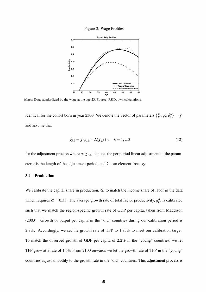
Figure 2: Wage Profiles
20 25 30 35 40 45 50 55 601
1.1
1.2
1.3
1.4
1.5
1.6
1.7
Age
Pro
duct
ivity
Productivity Profiles
Old CountriesYoung CountriesObserved US−Profile
Notes: Data standardized by the wage at the age 23. Source: PSID, own calculations.
identical for the cohort born in year 2300. We denote the vector of parameters {ξi,ψi,δ hi }= χi
and assume that
χi,k = χi= j,k +∆(χ j,k) · t k = 1,2,3, (12)
for the adjustment process where ∆(χ j,k) denotes the per period linear adjustment of the param-
eter, t is the length of the adjustment period, and k is an element from χi.
3.4 Production
We calibrate the capital share in production, α , to match the income share of labor in the data
which requires α = 0.33. The average growth rate of total factor productivity, gAi , is calibrated
such that we match the region-specific growth rate of GDP per capita, taken from Maddison
(2003). Growth of output per capita in the “old” countries during our calibration period is
2.8%. Accordingly, we set the growth rate of TFP to 1.85% to meet our calibration target.
To match the observed growth of GDP per capita of 2.2% in the “young” countries, we let
TFP grow at a rate of 1.5% From 2100 onwards we let the growth rate of TFP in the “young”
countries adjust smoothly to the growth rate in the “old” countries. This adjustment process is
20

assumed to be completed in 2300. Further, we compute relative GDP per capita from Maddison
(2003) for both regions in 1950 and use this ratio to calibrate the relative productivity levels at
the beginning of the calibration period. Initially, per capita GDP in the developing countries is
only 20% of income per capita in the industrialized nations. Finally, we calibrate δ such that
our simulated data match an average investment output ratio of 20% in the North which requires
δ = 0.035.
3.5 The Pension System
In our first social security scenario (“const. τ”) we fix contribution rates and adjust replacement
rates of the pension system. Since there is no yearly data on contribution rates for sufficiently
many countries, we use data from Palacios and Pallares-Miralles (2000) for the mid 1990s and
assume that the contribution rate was constant through the entire calibration period. On the
individual country level, we use the pension tax as a share of total labor costs weighted by the
share of contributing workers to compute a national average. Then we weight these numbers by
total GDP to compute a representative number for the two world regions. The contribution rate
in the “young” (“old”) region is then 4.1% (10.9%). Given the initial demographic structures,
the replacement rate is 13.8% (20.4%) in the “young” (“old”) region. In our baseline social
security scenario we freeze the contribution rate at the level used for the calibration period
for all following years. When simulating the alternative social security scenario with constant
replacement rates (“const. ρ”) we feed the equilibrium replacement rate obtained in the “const.
τ” scenario into the model and hold it constant at the level of year 2000 for all remaining
years.19 Then, the contribution rate endogenously adjusts each period to balance the budget of
the social security system. In both scenarios we assume that the retirement age is fixed at 65
years and agents do not expect any change. We label this scenario as “Benchmark” (“BM”) in
19The choice of year 2000 is motivated by the fact that this is the last year for which we had data on social security.
21
the following figures.
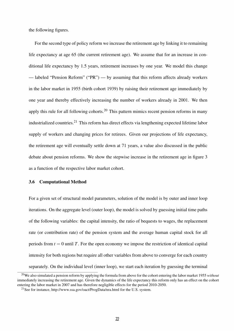
For the second type of policy reform we increase the retirement age by linking it to remaining
life expectancy at age 65 (the current retirement age). We assume that for an increase in con-
ditional life expectancy by 1.5 years, retirement increases by one year. We model this change
— labeled “Pension Reform” (“PR”) — by assuming that this reform affects already workers
in the labor market in 1955 (birth cohort 1939) by raising their retirement age immediately by
one year and thereby effectively increasing the number of workers already in 2001. We then
apply this rule for all following cohorts.20 This pattern mimics recent pension reforms in many
industrialized countries.21 This reform has direct effects via lengthening expected lifetime labor
supply of workers and changing prices for retirees. Given our projections of life expectancy,
the retirement age will eventually settle down at 71 years, a value also discussed in the public
debate about pension reforms. We show the stepwise increase in the retirement age in figure 3
as a function of the respective labor market cohort.
3.6 Computational Method
For a given set of structural model parameters, solution of the model is by outer and inner loop
iterations. On the aggregate level (outer loop), the model is solved by guessing initial time paths
of the following variables: the capital intensity, the ratio of bequests to wages, the replacement
rate (or contribution rate) of the pension system and the average human capital stock for all
periods from t = 0 until T . For the open economy we impose the restriction of identical capital
intensity for both regions but require all other variables from above to converge for each country
separately. On the individual level (inner loop), we start each iteration by guessing the terminal
20We also simulated a pension reform by applying the formula from above for the cohort entering the labor market 1955 withoutimmediately increasing the retirement age. Given the dynamics of the life expectancy this reform only has an effect on the cohortentering the labor market in 2007 and has therefore negligible effects for the period 2010-2050.
21See for instance, http://www.ssa.gov/oact/ProgData/nra.html for the U.S. system.
22

Figure 3: Retirement Age
1900 1950 2000 2050 2100 215063
64
65
66
67
68
69
70
71
72
73
Labor Market Cohort
Ret
irem
ent
Ag
e
Statutory Retirement Age
Benchmark (Constant Retirement)Pension Reform (Rising Retirment Age)
Notes: The jumps in the broken line indicate the cohort which is affected by the change in the retirement age and notthe actual time when the number of workers is increasing.
values for consumption and human capital. Then we proceed by backward induction and iterate
over these terminal values until convergence of the inner loop iterations. In each outer loop,
disaggregated variables are aggregated each period. We then update aggregate variables until
convergence using the Gauss-Seidel-Quasi-Newton algorithm suggested in Ludwig (2007).
To calibrate the model in the “const. τ” scenario, we consider additional “outer outer” loops
to determine structural model parameters by minimizing the distance between simulated aver-
age values and their respective calibration targets for the calibration period 1960− 2005. To
summarize the description above, parameter values determined in this way are β , ϕ , δ , and
{ξi,ψi,δ hi }.
4 Results
We divide the presentation of results into three parts. In the first part, in subsection 4.1, we look
at the evolution of economic aggregates such as the rate of return of detrended GDP per capita
along the transition. When we evaluate future trends of economic aggregates in this first part,
23

Table 1: Model Parameters
“Young” “Old”Preferences σ Inverse of Inter-Temporal Elasticity of Substitution 2.00
β Pure Time Discount Factor 0.985ϕ Weight of Consumption 0.370
Human Capital ξ Scaling Factor 0.176 0.166ψ Curvature Parameter 0.576 0.586δ h Depreciation Rate of Human Capital 1.4% 0.9%h0 Initial Human Capital Endowment 1.00 1.00
Production α Share of Physical Capital in Production 0.33δ Depreciation Rate of Physical Capital 3.5%gA Exogenous Growth Rate
Calibration Period 1.5% 1.9%Final Steady State 1.9% 1.9%
Notes: “Young” and “Old” refer to the region. Only one value in a column indicates that the parameter is identicalfor both regions.
we do so in two steps.
In our first step, we look at a comparison of open and counterfactual closed economy ver-
sions of our model for two pension scenarios (a “fixed contribution rate” and a “fixed replace-
ment rate” system) and two human capital scenarios (“exogenous” versus “endogenous” human
capital). What we learn from this exercise is that openness matters for the evolution of aggre-
gates such as GDP per capita but, probably surprisingly, not so much for rates of return. What
matters more for the time path of the latter is whether human capital is endogenous and how the
pension system is designed.
In our second step, we evaluate how our findings are affected by increasing the retirement
age. To distinguish increases in the retirement age semantically from the aforementioned pen-
sion “scenarios”, we label the experiment of increasing the retirement age as a “pension reform”
(“PR”). Given our findings from the first step, we focus our analysis only at the more realistic
and policy relevant open economy model version of our model. We find that increasing the
24

retirement age, by increasing labor supply and human capital, will significantly alter the time
path of future rates of return to capital and wages.
In the second part, subsection 4.2, we shed more light on how the increase in retirement age
affects effective labor supply. We ask how much of the exogenous increase in the retirement
age (extensive margin) is potentially offset by adverse endogenous labor supply reactions at
the intensive margin. Overall, we find little response at the intensive labor supply margin.
Consequently, increasing the retirement age is a very effective reform.
In the third part, subsection 4.3, we evaluate welfare of households who live through the
demographic transition and show that endogenous formation of human capital and the design
of the pension system are — via future time paths of wages and returns — key for the welfare
effects of aging. Consistently with the literature22, we find that, when the contribution rate
is held constant, increasing wages dominate for newborn households who experience welfare
gains whereby the converse applies to old and asset rich households. Gains of the young (and
losses of the old) are significantly higher (lower) when human capital can endogenously adjust
and when the retirement age increases. On the contrary, welfare differences between our closed
and open economy scenarios are small.
4.1 Macroeconomic Aggregates
Aggregate Variables for the Benchmark Model
Figures 4(a) and 4(b) depict the evolution of contribution and replacement rates for the bench-
mark pension system. Holding the replacement rate constant at 16.4% requires an increase of
the contribution rate to 18% in 2050. Conversely, keeping the contribution rate unchanged dur-
ing the entire period at 10.9% requires a drop in the replacement rate to 9.4% until 2050. Small
differences emanate in the graphs for the closed and open economy scenarios of our model.22E.g., Kruger and Ludwig (2007), Ludwig, Schelkle, and Vogel (2012).
25

These are induced by differential paths of wages and labor supply as well as human capital
formation in the respective model variants.
Figure 4: Adjustment of Pension System, Benchmark Pension System
(a) Replacement Rate
2010 2015 2020 2025 2030 2035 2040 2045 20509
10
11
12
13
14
15
16
17
Year
Rep
lace
men
t R
ate
in %
Replacement Rate
Constant τ, OpenConstant ρ, OpenConstant τ, ClosedConstant ρ, Closed
(b) Contribution Rate
2010 2015 2020 2025 2030 2035 2040 2045 205010
11
12
13
14
15
16
17
18
19
Year
Co
ntr
ibu
tio
n R
ate
in %
Contribution Rate
Constant τ, OpenConstant ρ, OpenConstant τ, ClosedConstant ρ, Closed
Notes: “Open” and “Closed” refer to the results obtained from the closed and open economy versions. All resultsobtained from the endogenous human capital scenario, benchmark pension system with constant retirement age(“BM”).
The evolution of important macroeconomic variables for the scenario with constant contribu-
tion rate (“const. τ”) is presented in figure 5. As in this subsection we concentrate on the model
comparison across capital market scenarios we report results for the alternative adjustment of
the pension system (“const. ρ”) in figure 10 in appendix B.
Figure 5(a) shows the evolution of the rate of return to physical capital for different model
variants. Looking at the development of the rate of return in a closed economy we observe the
well known result of falling returns due to population aging. However, we also observe that
the drop in the interest rate is much lower in the model where human capital is endogenous as
opposed to the “standard” model with an exogenously given life cycle productivity profile. This
effect is the result of higher investment into human capital due to falling returns to physical
capital. In the open economy variant, we observe a qualitatively similar result with two differ-
ences. As the “young” economy is importer of capital, the interest rate in the open economy is
26

initially higher than in the closed economy. This pattern is reversed after year 2030 when baby
boomers retire in the “old” economy and withdraw their funds (see below). Quantitatively,
initial differences are relatively small when human capital formation is endogenous.
We next report the level of de-trended GDP per capita in figure 5(d) where we have stan-
dardized the value for the year 2010 to 100. In both model versions with endogenous human
capital the income level in 2050 is by an economically significant amount above the level of
the “standard” model. This effect is due to more investment into human capital. Turning to the
comparison between closed and open economies we observe that income in 2050 in the open
economy tends to be higher compared to the closed economy (for endogenous and exogenous
human capital).
GDP per capita in the closed economy is initially higher than in the open economy. The
reason is the inflow and outflow of physical capital during the transition period. As can be seen
from figure 5(b), the “old” region has a positive net foreign asset position until 2035 (2040)
in the version with endogenous (exogenous) human capital. This initial outflow of capital de-
creases production at home and thereby GDP per capita. However, as the capital flows are
reversed and capital is repatriated, GDP per capita is surpassing the level of the closed econ-
omy.
These differences between the open and closed economy scenarios are most pronounced
when human capital adjusts. This can be seen in figure 5(c). Average human capital is higher
in the open economy compared to the closed economy after 2035. The initially lower time
investment into human capital accumulation in the open economy scenario can be attributed to
the lower wage growth and higher rate of return compared to the closed economy scenario. In
the closed economy, the demographic structure of the “old” economy leads to relatively more
pronounced accumulation of physical capital which can be only used domestically. Therefore,
27

opening up the economy and thereby exporting physical capital to regions with higher returns
is initially detrimental for investment into human capital at home.
Figure 5: Aggregate Variables for Constant Contribution Rate Scenario, Benchmark Pension System
(a) Rate of Return to Physical Capital
2010 2015 2020 2025 2030 2035 2040 2045 20506.8
7
7.2
7.4
7.6
7.8
8
Year
r in
%
Rate of Return
Endogenous, OpenEndogenous, ClosedExogenous, OpenExogenous, Closed
(b) Net Foreign Assets
2010 2015 2020 2025 2030 2035 2040 2045 2050−60
−40
−20
0
20
40
60
Year
For
eign
Ass
ets
/ GD
P
Foreign Assets as Percentage of GDP
EndogenousExogenous
(c) Average Human Capital
2010 2015 2020 2025 2030 2035 2040 2045 20502.2
2.3
2.4
2.5
2.6
2.7
2.8
2.9
Year
Ave
rag
e H
um
an C
apit
al
Average Human Capital
Endogenous, OpenEndogenous, ClosedExogenous, OpenExogenous, Closed
(d) Detrended GDP per Capita
2010 2015 2020 2025 2030 2035 2040 2045 205094
96
98
100
102
104
106
108
Year
Det
ren
ded
GD
P p
er C
apit
a
Detrended GDP per Capita
Endogenous, OpenEndogenous, ClosedExogenous, OpenExogenous, Closed
Notes: “Endogenous” and “Exogenous” refer to the human capital production profile. “Open” and “Closed” refer tothe results obtained from the closed and open economy versions. All results obtained from the constant contributionrate scenario, benchmark pension system with constant retirement age (“BM”).
The most striking result displayed in figure 5(d) is the increase of de-trended per capita GDP,
despite the seemingly detrimental effects of aging on raw labor supply. Endogenous human
capital formation in combination with a constant contribution rate pushes growth rates along
the transition above the long-run trend level of 1.8 percent. On the contrary, de-trended GDP
per capita decreases until about 2030 in the open economy when replacement rates are held
28

constant. In this case the associated increase in contribution rates — cf. figure 4(b) — reduces
incentives to invest in human capital, cf. figure 10 in appendix B.
Aggregate Variables when the Retirement Age is Increased
We now investigate how our results are affected once we let the retirement age increase accord-
ing to the pattern shown in figure 3. To focus our analysis, we do so in our benchmark open
economy model with endogenous human capital formation. We continue with our comparison
across the two pension designs – constant contribution and constant replacement rates.
Figure 6 displays the associated time paths of replacement and contribution rates. Observe
that, in case of a fixed contribution (replacement) rate, the base replacement (contribution) rate
is higher when the retirement age adjusts. This is so for mainly two reasons. First, there is
a higher exogenous amount of raw labor in the economy. Second, as shown below, higher
retirement ages increase the incentive to invest in human capital. Hence, also the quality of
labor is higher when retirement ages are raised. The figure also displays jumps in the relevant
variables. This is due to the fact that our smallest unit of time is one calendar year and it
is therefore not possible to implement more gradual changes in the retirement age leading to
smoother transitions.
Our results of this experiment on macroeconomic variables are summarized in figure 7. In-
creasing the retirement age has strong effects. The level of rates of returns are significantly
higher than in our benchmark scenario. This is so because of the aforementioned effects of
increasing the retirement age on total effective labor supply. As a consequence, even when re-
placement rates are held constant — and contribution rates adjust correspondingly — GDP per
capita is now found to increase.
Notice that in the endogenous human capital model the effect of increasing the retirement
29

Figure 6: Adjustment of Pension System, Pension Reform
(a) Constant Replacement Rate
2010 2015 2020 2025 2030 2035 2040 2045 20509
10
11
12
13
14
15
16
17
Year
Rep
lace
men
t R
ate
in %
Replacement Rate
Constant τ, BMConstant τ, PRConstant ρ, BMConstant ρ, PR
(b) Constant Contribution Rate
2010 2015 2020 2025 2030 2035 2040 2045 205010
11
12
13
14
15
16
17
18
19
Year
Co
ntr
ibu
tio
n R
ate
in %
Contribution Rate
Constant τ, BMConstant τ, PRConstant ρ, BMConstant ρ, PR
Notes: Results from the model with endogenous human capital and open capital markets.
age is stronger in the constant replacement rate scenario (e.g., compare panels (c) and (d) of
figure 7). To understand this, recall from figure 6 that the increase of contribution rates is
substantially dampened in the reform “PR”. The overall tax burden is therefore lowered which
induces additional incentives to invest in human capital. On the contrary, in the constant contri-
bution rate scenario, the replacement rate decreases by less. This just has the opposite incentive
effects on human capital formation.
In figure 11 in appendix B we plot changes in the same variables for the model with ex-
ogenous human capital. As expected, when human capital cannot adjust the effect of a higher
retirement age are generally found to be smaller.
4.2 Labor Supply over the Life Cycle
Key for understanding these adjustments at the aggregate level is the response of hours worked
and human capital formation over the life cycle. Theoretical insights on these life cycle effects
are developed in appendix B.2 by use of a simple two-period model. To shed light on these life
cycle adjustments quantitatively, we isolate the effects induced by a change in the retirement
30

Figure 7: Aggregate Variables in Open Economy Scenario, Benchmark vs. Pension Reform
(a) Rate of Return to Physical Capital, Constant τ
2010 2015 2020 2025 2030 2035 2040 2045 20507.5
7.6
7.7
7.8
7.9
8
8.1
Year
r in
%
Rate of Return
Endogenous, BMEndogenous, PR
(b) Rate of Return to Physical Capital, Constant ρ
2010 2015 2020 2025 2030 2035 2040 2045 20507.5
7.55
7.6
7.65
7.7
7.75
7.8
7.85
7.9
7.95
8
Yearr
in %
Rate of Return
Endogenous, BMEndogenous, PR
(c) Detrended GDP per Capita, Constant τ
2010 2015 2020 2025 2030 2035 2040 2045 2050100
102
104
106
108
110
112
114
Year
Det
ren
ded
GD
P p
er C
apit
a
Detrended GDP per Capita
Endogenous, BMEndogenous, PR
(d) Detrended GDP per Capita, Constant ρ
2010 2015 2020 2025 2030 2035 2040 2045 205094
96
98
100
102
104
106
108
110
112
Year
Det
ren
ded
GD
P p
er C
apit
a
Detrended GDP per Capita
Endogenous, BMEndogenous, PR
(e) Average Human Capital, Constant τ
2010 2015 2020 2025 2030 2035 2040 2045 2050
2.45
2.5
2.55
2.6
2.65
2.7
2.75
2.8
2.85
2.9
Year
Ave
rag
e H
um
an C
apit
al
Average Human Capital
Endogenous, BMEndogenous, PR
(f) Average Human Capital, Constant ρ
2010 2015 2020 2025 2030 2035 2040 2045 20502.3
2.35
2.4
2.45
2.5
2.55
2.6
2.65
2.7
2.75
2.8
Year
Ave
rag
e H
um
an C
apit
al
Average Human Capital
Endogenous, BMEndogenous, PR
Notes: Results from the model with endogenous human capital and open capital markets.
31

age from changes induced by general equilibrium feedback. First, we define our benchmark to
be the cohort entering the labor market in 1955. This is the first cohort affected by an increase
of the normal retirement age. Then, we take general equilibrium prices and policy instruments
from the benchmark economy (with retirement age 65) and increase the retirement age. This
enables us to compare household decisions in partial equilibrium. In order to isolate the dif-
ferent adjustment channels — labor supply and human capital — in this partial equilibrium
setting we perform three experiments. We start by holding constant the human capital profile of
the benchmark cohort from the benchmark social security scenario and endogenously compute
labor supply. We next hold the labor supply profile fixed and allow human capital to adjust.
Finally, we allow labor supply and human capital to be endogenous and thereby capture the
total effect (in partial equilibrium). As a last step, we compare our results to the life cycle pro-
files of households observed in general equilibrium after implementation of the pension reform.
This profile includes endogenous adjustments of labor, human capital, and prices. Using this
procedure we can identify the most important drivers of our results at the household level.
Results on this decomposition analysis are summarized in figure 8 as percent deviations from
the benchmark life cycle profile. Ignoring general equilibrium adjustments and human capital
accumulation, an increase in the retirement age has a negligible impact on labor supply at the
intensive margin. With both margins of adjustment at work (“both endogenous”) the young
invest more time in education and hence labor supply decreases relative to the benchmark. Older
agents work more to reap the benefits of higher levels of human capital. These predictions are
consistent with equation (29). Finally, in general equilibrium, the endogenous labor supply
and human capital response leads to higher pension payments, lower increase in wages and
relatively higher interest rates. This mitigates the incentives to invest into human capital and
increases (decreases) labor supply when young (old) relative to the case with constant prices.
32

As a consequence, once all general equilibrium adjustments are considered, incentives to work
and invest into human capital are weakened and lead only to a small change of labor supply on
the intensive margin.
Figure 8: Reallocation over the Life Cycle with PR, Partial vs. General Equilibrium
(a) Change in Labor Supply, Constant τ
10 20 30 40 50 60 70−3
−2
−1
0
1
2
3
4
5
Age
Cha
nge
in P
erce
nt
Change of Labor Supply Relative to Benchmark, const. τ
Labor EndogenousBoth EndogenousGE − Effect
(b) Change in Human Capital, Constant τ
10 20 30 40 50 60 700
0.5
1
1.5
2
2.5
Age
Cha
nge
in P
erce
nt
Change of Human Capital Relative to Benchmark, const. τ
HC EndogenousBoth EndogenousGE − Effect
Notes: “Endogenous” and “Exogenous” refer to the human capital production profile. Results with open capitalmarkets.
Table 2 documents the total effect of these behavioral adjustments as the sum of changes of
life cycle allocations shown in the previous figure. Moving from left to right in the table, we
observe a reaction of labor supply at the intensive margin in partial equilibrium only when edu-
cation and hours worked are simultaneously endogenous. This is offset in general equilibrium.
We can therefore conclude that the exogenous increase of the retirement age has a strong impact
on total aggregate effective labor supply only by inducing agents to work more in the marginal
year and investing more into human capital. On the contrary, reactions at the intensive margin
only shift allocations over the life cycle without affecting the aggregate much.23
23With the exception of the first few years after the reform during which increased human capital investments through eductioncrowd out labor supply. The effect is, however, small and therefore not shown.
33
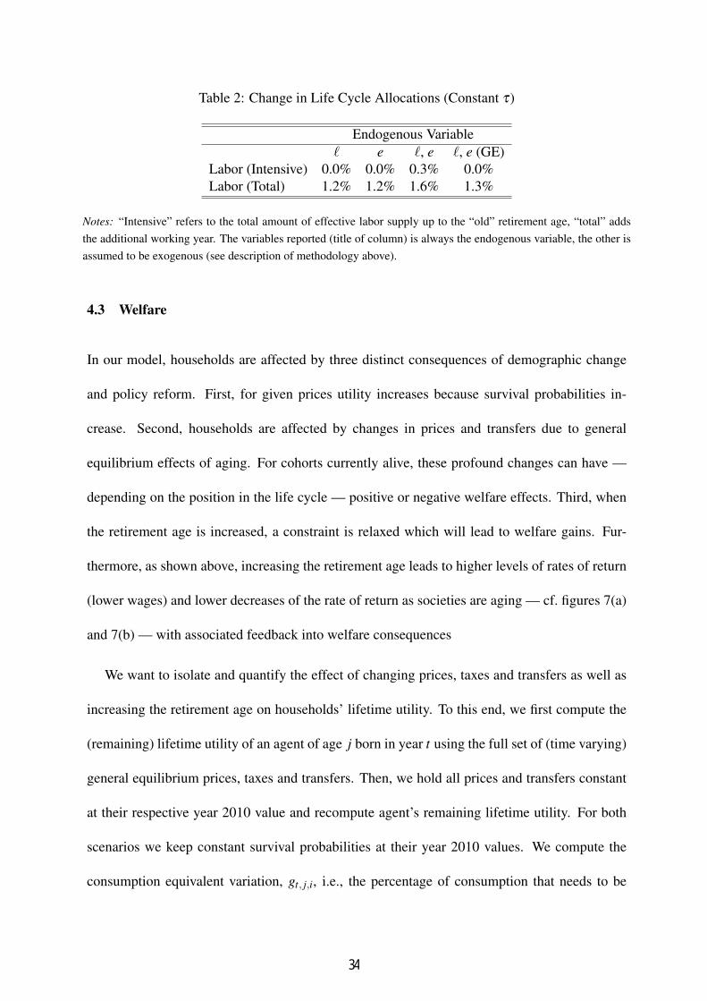
Table 2: Change in Life Cycle Allocations (Constant τ)
Endogenous Variableℓ e ℓ, e ℓ, e (GE)
Labor (Intensive) 0.0% 0.0% 0.3% 0.0%Labor (Total) 1.2% 1.2% 1.6% 1.3%
Notes: “Intensive” refers to the total amount of effective labor supply up to the “old” retirement age, “total” addsthe additional working year. The variables reported (title of column) is always the endogenous variable, the other isassumed to be exogenous (see description of methodology above).
4.3 Welfare
In our model, households are affected by three distinct consequences of demographic change
and policy reform. First, for given prices utility increases because survival probabilities in-
crease. Second, households are affected by changes in prices and transfers due to general
equilibrium effects of aging. For cohorts currently alive, these profound changes can have —
depending on the position in the life cycle — positive or negative welfare effects. Third, when
the retirement age is increased, a constraint is relaxed which will lead to welfare gains. Fur-
thermore, as shown above, increasing the retirement age leads to higher levels of rates of return
(lower wages) and lower decreases of the rate of return as societies are aging — cf. figures 7(a)
and 7(b) — with associated feedback into welfare consequences
We want to isolate and quantify the effect of changing prices, taxes and transfers as well as
increasing the retirement age on households’ lifetime utility. To this end, we first compute the
(remaining) lifetime utility of an agent of age j born in year t using the full set of (time varying)
general equilibrium prices, taxes and transfers. Then, we hold all prices and transfers constant
at their respective year 2010 value and recompute agent’s remaining lifetime utility. For both
scenarios we keep constant survival probabilities at their year 2010 values. We compute the
consumption equivalent variation, gt, j,i, i.e., the percentage of consumption that needs to be
34

given to the agent at each date for her remaining lifetime at prices from 2010 in order to make
her indifferent between the two scenarios. Positive values of gt, j,i thus indicate welfare gains
from the general equilibrium effects of aging.24 In order to isolate the effects of changing
prices, taxes and transfers, we do not account for the gain in households’ lifetime utility during
the additional life years generated by the increase in life expectancy.
In the remainder of this section we stick to the structure from the previous section. We first
report numbers from our welfare analysis for agents living in the benchmark pension scenario
holding the retirement age constant. Then we advance to the comparison of the effects of
increasing the retirement age. To work out distributional consequences across generations, we
first look at welfare consequences for agents alive in 2010, followed by an analysis of welfare
of future generations.
Welfare of Generations Alive in 2010 in the Benchmark Model
The analysis in this section performs an inter-generational welfare comparison of the conse-
quences of demographic change holding the retirement age at the current level. The results
for the “const ρ” (“const τ”) scenario are shown in figures 9(a) and 9(b). They can be sum-
marized as follows: for constant contribution rates, newborns in the endogenous (exogenous)
model benefit up to 0.7% (0.4%) of lifetime consumption from the general equilibrium effects
of aging. This is due to increasing wages and decreasing interest rates. Higher wage growth
makes investment into human capital more attractive and falling interest rates decrease the costs
of borrowing. Middle aged agents with high levels of physical assets incur welfare losses due
to falling interest rates. Further, their ability to change human capital investment is restricted
as they are in a relatively advanced stage of their life cycle. Retired agents additionally incur
24Using the functional form from equation (1) the consumption equivalent variation is given by gt, j,i =
(Vt, j,i
V 2010j
) 1ϕ(1−σ)
− 1
where Vt, j,i denotes lifetime utility using general equilibrium prices and V 2010j is lifetime utility using constant prices from 2010.
35

losses from falling pensions (due to constant contribution rates).
Figure 9: Consumption Equivalent Variation of Agents alive in 2010, Benchmark Pension System
(a) Constant Replacement Rate
10 20 30 40 50 60 70 80 90−4
−3.5
−3
−2.5
−2
−1.5
−1
−0.5
0
0.5
Age
CE
V
Consumption Equivalent Variation − Cohorts alive in 2010
Endogenous, OpenExogenous, Open
(b) Constant Contribution rate
10 20 30 40 50 60 70 80 90−7
−6
−5
−4
−3
−2
−1
0
1
Age
CE
V
Consumption Equivalent Variation − Cohorts alive in 2010
Endogenous, OpenExogenous, Open
Notes: “Endogenous” and “Exogenous” refer to the human capital production profile. Results from the model withendogenous human capital and open capital markets.
Of particular interest is that agents in the endogenous human capital investment model incur
much lower losses compared to households with a fixed human capital profile. With endogenous
human capital, maximum losses are about 32% lower compared to the model with a fixed human
capital profile. Thus, agents with the possibility to react to changing prices will do so and this
decreases their potential losses by a considerable amount.
On the contrary, openness per se does not have strong effects on welfare. This is directly
related to our insights from the previous part where we have shown that time paths of rates of
return to physical capital (and thereby wages) do not differ much between our open and our
counterfactual closed economy scenario. Welfare results for the closed economy are shown in
figure 12 in appendix B.
In the constant replacement rate scenario the majority of the population loses from the effects
of demographic change. Young agents are worse off as constant replacement rates require rising
36

contributions which depresses net wages and incentives to invest in human capital. Very old
agents experience small gains in lifetime utility due to rising pensions. Also notice that welfare
consequences are more evenly distributed under constant replacement rates where maximum
losses are considerably smaller than with constant contribution rates.25
We also summarize welfare consequences for newborns in our benchmark economy with
open capital markets in table 3 and the maximum welfare losses in table 4. Results for the
closed economy and can be found in appendix B in tables 5 and 6.
Table 3: Welfare Gains / Losses - Newborns 2010
Open EconomyPension System Constant τ Constant ρ
Endog. Exog. Endog. Exog.BM 0.8% 0.3% -3.0% -3.2%PR 1.2% 0.6% -1.7% -2.3%
Notes: “Endog.” and “Exog.” refer to the endogenous and exogenous human capital production profile. Resultsfrom the open economy scenario. “BM” denotes the benchmark pension system (constant retirement age), and “PR”denotes the pension reform (increase in the retirement age).
Table 4: Maximum Welfare Losses - Agents alive 2010
Open EconomyPension System Constant τ Constant ρ
Endog. Exog. Endog. Exog.BM -4.4% -6.5% -3.0% -3.6%PR -3.6% -6.0% -1.9% -3.0%
Notes: “Endog.” and “Exog.” refer to the endogenous and exogenous human capital production profile. Resultsfrom the open economy scenario.“BM” denotes the benchmark pension system (constant retirement age), and “PR”denotes the pension reform (increase in the retirement age).
25See Glomm and Kaganovich (2008) for the relationship between changes in social security, public education and welfare ina heterogenous agents model.
37

Welfare of Generations Alive in 2010 when the Retirement Age is Increased
We next look at differences in welfare changes for agents living in 2010 across all pension
reform scenarios. For sake of brevity, we focus on the summary of results in tables 3 and 4
and relegate the corresponding figure 13 to appendix B. Gains to newborn households increase
by 0.3 to 0.4 percentage points under constant replacement rates and losses decrease by more
than one percentage point under constant replacement rates.26
Welfare of Future Generations in the Benchmark Model
We now report welfare changes for newborns between 2010 and 2050, see figure 14 in ap-
pendix B. Holding the replacement rate constant has a strong negative impact on lifetime utility
for future generations. Even with endogenous investment into human capital, maximum welfare
losses can be up to 7% (5.9%) in the open (closed) economy. With an exogenous efficiency pro-
file, losses are even higher. With constant contribution rates, newborns gain up to 2.5% (1.5%)
in the open (closed) economy and endogenous human capital investment.
Welfare of Future Generations when the Retirement Age is Increased
In case of constant replacement rates, increasing the retirement age cannot totally eliminate
welfare losses from demographic change, see figure 15 in appendix B. However, the effect is
strong. In case of endogenous human capital, welfare losses of the cohort born in 2050 are now
at −2.6%, compared to −5.9% without the reform.
26GDP per capita and welfare increase due to higher capital accumulation and exogenous technical progress. Our methodologyto measure general equilibrium feedback effects, however, neglects these effects as we compare changing with constant prices(“purged” from aging induced effects) for any level of GDP per capita. In other words, for any cohort aggregate states (e.g. levelof GDP per capita) are identical in both scenarios at the beginning of the life-cycle but prices diverge later on.
38

5 Conclusion
This paper revisits the literature on the consequences of demographic change – aging – for wel-
fare of generations who live through the demographic transition in industrialized countries by
asking a straightforward question: How can the potentially detrimental consequences of aging
be mitigated by two margins of adjustment: investing abroad and human capital formation. We
address this question in combination with pension policy. That is, we ask how the design of
pension policy may contribute to dampening via these endogenous channels.
We conclude with a negative and a positive finding. Our negative finding is that openness
to international capital markets has only modest welfare implications vis-vis a counterfactual
closed economy world. The reason for this is that overall demographic trends across our two
highly aggregate world regions are very similar (despite strong differences in levels and the
heterogeneity within each region). To the extent that the group of industrialized countries is
relatively open to the rest of the world already today, this leads to relatively small price changes
over time when we contrast an open economy scenario with a counterfactual closed economy
scenario. Small price differences in turn lead to small welfare changes.
Our positive finding is that endogenous human capital formation in combination with con-
stant contribution rates to the pension system and increases of the statutory retirement age has
strong welfare effects. We find that, in general equilibrium, the exogenous increase of the re-
tirement age translates almost one for one into labor market participation of the elderly while
there is almost no reaction at the intensive margin of those already working. Hence, “reform
backlashes” (Borsch-Supan and Ludwig 2009) are small and effective labor supply is conse-
quently increased quite strongly. This leads to strong welfare gains for all future generations
(under constant contribution rates). Welfare losses for middle aged and asset rich households
39

who suffer from decreasing returns on savings and decreasing pension payments are 6.5% if
human capital cannot adjust and if the statutory retirement age is held constant. These losses
decrease to 3.6% if human capital endogenously adjusts and increases of the retirement age
roughly track life expectancy.
Our main conclusion from our analysis is therefore that labor market policies focusing at
the extensive margin (=increasing the retirement age) and adjustments at the intensive margin
(=human capital) are key vehicles to mitigate the adverse effects of demographic change. With
regard to human capital adjustments, we have, however, operated in a frictionless environment.
All endogenous human capital adjustments are driven by relative price changes, increases in life
expectancy and increases of the statutory retirement age. If, instead, human capital formation
is affected by market imperfections, such as borrowing constraints, then these automatic adjust-
ments will be inhibited. In this case, appropriate human capital policies in combination with
pension policies are an important topic for future research and the policy agenda.
40

References
Altig, David, Alan J. Auerbach, Laurence J. Kotlikoff, Kent A. Smetters, and Jan Walliser(2001). Simulating Fundamental Tax Reform in the United States. American EconomicReview 91(3), 574–594.
Arrazola, Maria and Jose de Hevia (2004). More on the estimation of the human capitaldepreciation rate. Applied Economic Letters 11, 145–148.
Attanasio, Orazio, Sagiri Kitao, and Giovanni L. Violante (2007). Global DemographicTrends and Social Security Reform. Journal of Monetary Economics 54(1), 144–198.
Auerbach, Alain J. and Laurence J. Kotlikoff (1987). Dynamic Fiscal Policy. Cambridge:Cambridge University Press.
Ben-Porath, Yoram (1967). The Production of Human Capital and the Life Cycle of Earnings.Journal of Political Economy 75(4), 352–365.
Borsch-Supan, Axel and Alexander Ludwig (2009). Living Standards in an Aging Germany:The Benefits of Reforms and the Costs of Resistance. Journal of Economics and Statis-tics 229(2-3), 163–179.
Borsch-Supan, Axel and Anette Reil-Held (2001). How Much Is Transfer and How MuchIs Insurance in a Pay-as-You-Go System? The German Case. Scandinavian Journal ofEconomics 103(3), 505–524.
Bosch-Supan, Axel, Alexander Ludwig, and Joachim Winter (2006). Ageing, Pension Re-form and Capital Flows: A Multi-Country Simulation Model. Economica 73, 625–658.
Broner, Fernando, Tatiana Didier, Aitor Erce, and Sergio L. Schmukler (2011). Gross CapitalFlows: Dynamics and Crises. mimeo.
Browning, Martin, Lars Peter Hansen, and James J. Heckman (1999). Micro Data and Gen-eral Equilibrium Models. In J. B. Taylor and M. Woodford (Eds.), Handbook of Macroe-conomics, Chapter 8, pp. 543–633. Amsterdam: Elsevier.
Buiter, Willem H. and Kenneth M. Kletzer (1995). Permanent International ProductivityGrowth Differentials in an Integrated Global Economy. Scandinavian Journal of Eco-nomics 95(4), 467–493.
Buyse, Tim, Freddy Heylen, and Renaat Van de Kerckhove (2012). Pension reform, employ-ment by age, and long-run growth. Journal of Population Economics, forthcoming.
De Nardi, Mariacristina, Selahattin Imrohoroglu, and Thomas J. Sargent (1999). ProjectedU.S. Demographics and Social Security. Review of Economic Dynamics 2(1), 575–615.
Diamond, Peter and Johathan Gruber (1999). Social Security and Retirement in the UnitedStates. In J. Gruber and D. Wise (Eds.), Social Security and Retirement Around the World,Chapter 11, pp. 437–474. Chicago: University of Chicago Press.
Domeij, David and Martin Floden (2006). Population Aging and International Capital Flows.International Economic Review 47(3), 1013–1032.
Fehr, Hans, Sabine Jokisch, and Laurence J. Kotlikoff (2005). Will China eat our lunch ortake us out for dinner? Simulating the transition paths of the U.S., EU, Japan, and China.NBER Working Paper No. 11668.
Fougere, Maxime and Marcel Merette (1999). Population Ageing and Economic Growth inSeven OECD Countries. Economic Modelling 16, 411–427.
French, Eric and John Jones (2012). Public pensions and labor supply over the life cycle.International Tax and Public Finance, 1–20. forthcoming.
41

Fuster, Luisa, Ayse Imrohoroglu, and Selahattin Imrohoroglu (2007). Elimination of SocialSecurity in a Dynastic Framework. Review of Economic Studies 74(1), 113–145.
Glomm, Gerhard and Michael Kaganovich (2008). Social security, public education and thegrowth-inequality relationship. European Economic Reviw 6(52), 1009–1034.
Gourieroux, Christian, Alain Monfort, and Eric Renault (1993). Indirect Inference. Journalof Applied Econometrics 8, S85–S118.
Guvenen, Fatih and Burhanettin Kuruscu (2009). A Quantitative Analysis of the Evolutionof the U.S. Wage Distribution: 1970-2000. In NBER Macroeconomics Annual. NBER.forthcoming.
Hall, Robert (1988). Intertemporal Substitution in Consumption. Journal of Political Econ-omy 96(2), 339–357.
Hansen, Gary D. (1993). The Cyclical and Secular Behaviour of the Labour Input: Compar-ing Efficiency Units and Hours Worked. Journal of Applied Econometrics 8(1), 71–80.
Hanushek, Eric A. and Dennis D. Kimko (2000). Schooling, Labor-Force Quality, and theGrowth of Nations. American Economic Review 90(2), 1184–1208.
Heckman, James, Lance Lochner, and Christopher Taber (1998). Explaining Rising WageInequality: Explorations with a Dynamic General Equilibrium Model of Labor Earningswith Heterogenous Agents. Review of Economic Dynamics 1, 1–58.
Huang, He, Selahattin Imrohoroglu, and Thomas J. Sargent (1997). Two Computations toFund Social Security. Macroeconomic Dynamics 1(1), 7–44.
Huggett, Mark, Gustavo Ventura, and Amir Yaron (2012). Sources of Lifetime Inequality.American Economic Review 101(7), 2923–54.
Hurd, Michael and Susann Rohwedder (2011). Trends in Labor Force Participation: HowMuch is Due to Changes in Pensions? Population Ageing 4, 81–96.
Imrohoroglu, Selahattin and Sagiri Kitao (2009). Labor supply elasticity and social securityreform. Journal of Public Economics 93(7-8), 867–878.
Imrohoroglu, Ayse, Selahattin Imrohoroglu, and Douglas Hugh Joines (1995). A Life CycleAnalysis of Social Securtiy. Economic Theory 6, 83–114.
Kruger, Dirk and Alexander Ludwig (2007). On the Consequences of Demographic Changefor Rates of Returns to Capital, and the Distribution of Wealth and Welfare. Journal ofMonetary Economics 54(1), 49–87.
Lane, Philip R. and Gian Maria Milesi-Ferretti (2007). The external wealth of nations markII: Revised and extended estimates of foreign assets and liabilities, 1970-2004. Journalof International Economics 73, 223–250.
Liao, Pei-Ju (2011). Does demographic change matter for growth? European EconomicReview 55(5), 659–677.
Ludwig, Alexander (2007). The Gauss-Seidel-Quasi-Newton Method: A Hybrid Algorithmfor Solving Dynamic Economic Models. Journal of Economic Dynamics and Con-trol 31(5), 1610–1632.
Ludwig, Alexander, Thomas Schelkle, and Edgar Vogel (2012). Demographic Change, Hu-man Capital and Welfare. Review of Economic Dynamics 15(1), 94–107.
Maddison, Angus (2003). The World Economy: Historical Statistics. Paris: OECD.Mastrobuoni, Giovanni (2009). Labor Supply Effects of the Recent Social Security Ben-
efit Cuts: Empirical Estimates Using Cohort Discontinuities. Journal of Public Eco-nomics 93(11-12), 1224–1233.
42

Oeppen, Jim and James W. Vaupel (2002). Broken Limits to Life Expectancy. Sci-ence 296(5570), 1029–1031.
Palacios, Robert and Montserrat Pallares-Miralles (2000). International Patterns of PensionProvision. World Bank Social Protection Discussion Paper Series No. 9.
Reinhart, Carmen M. and Kenneth S. Rogoff (2008). This time is different: A panoramicview of eight centuries of financial crisis. NBER Working Paper 13882.
Sadahiro, Akira and Manabu Shimasawa (2002). The Computable Overlapping GenerationsModel with Endogenous Growth Mechanism. Economic Modelling 20, 1–24.
Smith, Anthomy A. (1993). Estimating Nonlinear Time-Series Models Using Simulated Vec-tor Autoregressions. Journal of Applied Econometrics 8, S63–S84.
Storesletten, Kjetil (2000). Sustaining Fiscal Policy through Immigration. Journal of Politi-cal Economy 108(2), 300–323.
United Nations (2007). World Population Prospects: The 2002 Revision. United NationsPopulation Division. New York.
Whitehouse, Edward R. (2003). The Value of Pension Entitlements: A Model of Nine OECDcountries. OECD Social, Employment and Migration Working Papers No. 9.
43

A Computational Appendix
A.1 Household Problem
To simplify the description of the solution of the household model for given prices (wage andinterest rate), transfers and social security payments, we focus on steady states and thereforedrop the time index t and the country index i. Furthermore, we focus on a de-trended versionof the household problem in which all variables x are transformed to x = x
A where A is thetechnology level growing at the exogenous rate g. To simplify notation, we do not denotevariables by the symbol · but assume that the transformation is understood. The de-trendedversion of the household problem is then given by
V (a,h, j) = maxc,ℓ,e,a′,h′
{u(c,1− ℓ− e)+β s(1+g)ϕ(1−σ)V (a′,h′, j+1)
}s.t.
a′ =1
1+g((a+ tr)(1+ r)+ y− c)
y =
{ℓhw(1− τ) if j < jrp if j ≥ jr
h′ = g(h,e) (13)ℓ ∈ [0,1], e ∈ [0,1].
Here, g(h,e) is the human capital technology.
Let β = β s(1+ g)ϕ(1−σ) be the transformation of the discount factor. Using the budgetconstraints, now rewrite the above as
V (a,h, j) = maxc,ℓ,e,a′,h′
{u(c,1− ℓ− e)+ βV
(1
1+g((a+ tr)(1+ r)+ y− c) ,g(h,e), j+1
)}s.t.ℓ≥ 0.
where we have also replaced the bounded support of time investment and leisure with a one-sideconstraint on ℓ because the upper constraints, ℓ= 1, respectively e = 1, and the lower constraint,e = 0, are never binding due to Inada conditions on the utility function and the functional formof the human capital technology (see below). Denoting by µℓ the Lagrange multiplier on theinequality constraint for ℓ, we can write the first-order conditions as
c : uc − β1
1+gVa′(a
′,h′; j+1) = 0 (14a)
ℓ : −u1−ℓ−e + βhw(1− τ)1
1+gVa′(a
′,h′, j+1)+µℓ = 0 (14b)
e : −u1−ℓ−e + βgeVh′(a′,h′, j+1) = 0 (14c)
and the envelope conditions read as
a : Va(a,h, j) = β1+ r1+g
Va′(a′,h′, j+1) (15a)
h : Vh(a,h, j) = β(ℓw(1− τ)
11+g
Va′(a′,h′, j+1)+ghVh′(a
′,h′, j+1)). (15b)
44

Note that for the retirement period, i.e. for j ≥ jr, equations (14b) and (14c) are irrelevant andequation (15b) has to be replaced by
Vh(a,h, j) = βghVh′(a′,h′, j+1).
From (14a) and (15a) we get
Va = (1+ r)uc (16)
and, using the above in (14a), the familiar inter-temporal Euler equation for consumption fol-lows as
uc = β1+ r1+g
uc′ . (17)
From (14a) and (14b) we get the familiar intra-temporal Euler equation for leisure,
u1−ℓ−e = hw(1− τ)uc +µℓ. (18)
From the human capital technology (3) we further have
ge = ξ ψ(eh)ψ−1h (19a)
gh = (1−δ h)+ξ ψ(eh)ψ−1e. (19b)
We loop backwards in j from j = J−1, . . . ,0 by taking an initial guess of [cJ,hJ] as given andby initializing Va′(·,J) =Vh′(·,J) = 0. During retirement, that is for all ages j ≥ jr, our solutionprocedure is by standard backward shooting using the first-order conditions. However, duringthe period of human capital formation, that is for all ages j < jr, the first order conditions wouldnot be sufficient if the problem is not a convex-programming problem. And thus, our backwardshooting algorithm will not necessarily find the true solution. In fact this may be the case inhuman capital models such as ours because the effective wage rate is endogenous (it dependson the human capital investment decision). For a given initial guess [cJ,hJ] we therefore firstcompute a solution via first-order conditions and then, for each age j < jr, we check whetherthis is the unique solution. As an additional check, we consider variations of initial guessesof [cJ,hJ] on a large grid. In all of our scenarios we never found any multiplicities.
The details of our steps are as follows:
1. In each j, h j+1,Va′(·, j+1),Vh′(·, j+1) are known.
2. Compute uc from (14a).
3. For j ≥ jr, compute h j from (3) by setting e j = ℓ j = 0 and by taking h j+1 as given andcompute c j directly from equation (23) below.
4. For j < jr:
(a) Assume ℓ ∈ [0,1) so that µℓ = 0.(b) Combine (3), (14b), (14c) and (19a) to compute h j as
h j =1
1−δ h
h j+1 −ξ
(ξ ψ 1
1+gVh′(·, j+1)
ω(1− τ)Va′(·, j+1)
) ψ1−ψ (20)
45

(c) Compute e from (3) as
e j = 1h j
(h j+1−h j(1−δ h)
ξ
) 1ψ. (21)
(d) Calculate lcr j =1−e j−ℓ j
c j, the leisure to consumption ratio from (18) as follows: From
our functional form assumption on utility marginal utilities are given by
uc =(
cϕ (1− ℓ− e)1−ϕ)−σ
ϕcϕ−1(1− ℓ− e)1−ϕ
u1−ℓ−e =(
cϕ (1− ℓ− e)1−ϕ)−σ
(1−ϕ)cϕ (1− ℓ− e)−ϕ
hence we get from (18) the familiar equation:
u1−ℓ−e
uc= hw(1− τ) =
1−ϕϕ
c1− ℓ− e
,
and therefore:
lcr j =1− e j − ℓ j
c j=
1−ϕϕ
1hw(1− τ)
. (22)
(e) Next compute c j as follows. Notice first that one may also write marginal utility fromconsumption as
uc = ϕcϕ(1−σ)−1(1− ℓ− e)(1−σ)(1−ϕ). (23)
Using (22) in (23) we then get
uc = ϕcϕ(1−σ)−1(lcr · c)(1−σ)(1−ϕ)
= ϕc−σ · lcr(1−σ)(1−ϕ). (24)
Since uc is given from (14a), we can now compute c as
c j =
uc j
ϕ · lcr(1−σ)(1−ϕ)j
− 1σ
. (25)
(f) Given c j, e j compute labor, ℓ j, as
ℓ j = 1− lcr j · c j − e j.
(g) If ℓ j < 0, set ℓ j = 0 and iterate on h j as follows:i. Guess h j
ii. Compute e as in step 4c.iii. Noticing that ℓ j = 0, update c j from (23) as
c =(
uc
ϕ(1− e)(1−σ)(1−ϕ)
) 1ϕ(1−σ)−1
.
iv. Compute µℓ from (14b) as
µℓ = u1−ℓ−e − βhw(1− τ)Va′(·, j+1)
46

v. Finally, combining equations (14b), (14c) and (19a) gives the following distancefunction f
f = e−
(β ξ ψhψ 1
1+gVh′(·)βωh(1− τ)Va′(·)+µℓ
) 11−ψ
, (26)
where e is given from step 4(g)ii. We solve for the root of f to get h j by a non-linear solver iterating on steps 4(g)ii through 4(g)v until convergence.
5. Update as follows:
(a) Update Va using either (15a) or (16).(b) Update Vh using (15b).
Next, loop forward on the human capital technology (3) for given h0 and {e j}Jj=0 to compute
an update of hJ denoted by hnJ . Compute the present discounted value of consumption, PVC,
and, using the already computed values {hnj}J
j=0, compute the present discounted value of in-come, PV I. Use the relationship
cn0 = c0 ·
PV IPVC
(27)
to form an update of initial consumption, cn0, and next use the Euler equations for consumption
to form an update of cJ , denoted as cnJ . Define the distance functions
g1(cJ,hJ) = cJ − cnJ (28a)
g2(cJ,hJ) = hJ −hnJ . (28b)
In our search for general equilibrium prices, constraints of the household model are occasionallybinding. Therefore, solution of the system of equations in (28) using Newton based methods,e.g., Broyden’s method, is instable. We solve this problem by a nested Brent algorithm, that is,we solve two nested univariate problems, an outer one for cJ and an inner one for hJ .
Check for uniqueness: Observe that our nested Brent algorithm assumes that the functionsin (28) exhibit a unique root. As we adjust starting values [cJ,hJ] with each outer loop iterationwe thereby consider different points in a variable box of [cJ,hJ] as starting values. For all ofthese combinations our procedure always converged. To systematically check whether we alsoalways converge to the unique optimum, we fix, after convergence of the household problem, alarge box around the previously computed [cJ,hJ]. Precisely, we choose as boundaries for thisbox ±50% of the solutions in the respective dimensions. For these alternative starting valueswe then check whether there is an additional solution to the system of equations (28). We neverdetected any such multiplicities.
A.2 The Aggregate Model
To solve the open economy general equilibrium transition path we proceed as follows: for agiven r × 1 vector Ψ of structural model parameters, we first solve for an “artificial” initialsteady state in period t = 0 which gives initial distributions of assets and human capital. Wethereby presume that households assume prices to remain constant for all periods t ∈ {0, . . . ,T}and are then surprised by the actual price changes induced by the transitional dynamics. Next,we solve for the final steady state of our model which is reached in period T and supported by
47

our demographic projections. In the sequel, the superscripts c and o refer to the closed or openeconomy and M denotes the number of regions.
For the closed economy steady state, for each region j we solve for the equilibrium of theaggregate model by iterating on the mc×1 steady state vector Pc
ss, j =[p1, j, . . . , pmc, j
]′. p1, j is thecapital intensity, p2, j are transfers (as a fraction of wages), p3, j are social security contribution(or replacement) rates and p4, j is the average human capital stock for region j. We perform thisprocedure separately for both world regions.
To compute the open economy steady state we solve for the equilibrium of the aggregatemodel by iterating on the mo ×1 steady state vector Po
ss =[p1, . . . , pmo, j
]′ where the number ofvariables is given by mo = M(mc −1)+1. p1 is the common (world) capital intensity, p2, j aretransfers (as a fraction of wages), p3, j are social security contribution (or replacement) rates andp4, j is the average human capital stock for region j. Notice that all elements of Pc
ss and Poss are
constant in the steady state.
Solution for the steady states for each closed region j (where we drop the region index forbrevity) of the model involves the following steps:
1. In iteration q for a guess of Pc,qss solve the household problem.
2. Update variables in Pcss as follows:
(a) Aggregate across households to get aggregate assets and aggregate labor supply toform an update of the capital intensity, pn
1.(b) Calculate an update of bequests to get pn
2.(c) Using the update of labor supply, update social security contribution (or replacement)
rates to get pn3.
(d) Use labor supply and human capital decisions to form an update of the average humancapital stock, pn
4.
3. Collect the updated variables in Pc,nss and notice that Pc,n
ss = H(Pcss) where H is a vector-
valued non-linear function.
4. Define the root-finding problem G(Pcss) = Pc
ss−H(Pcss) and iterate on Pc
ss until convergence.We use Broyden’s method to solve the problem and denote the final approximate Jacobimatrix by Bss.
Solution for the steady states of the open economy of the model involves the following steps:
1. In iteration q for a guess of Po,qss solve the household problem.
2. Update variables in Poss as follows:
(a) Use the guess for the global capital intensity to compute the capital stock for regionj compatible with the open economy, perfect competition setup. Use this aggregatecapital stock with the aggregate labor supply to form an update of the global capitalintensity, pn
1.(b) Calculate an update of bequests to get pn
2, j ∀ j.(c) Using the update of labor supply, update social security contribution (or replacement)
rates to get pn3, j ∀ j.
(d) Use labor supply and human capital decisions to form an update of the average humancapital stock, pn
4 ∀ j.
48

3. Collect the updated variables in Po,nss and notice that Po,n
ss = H(Poss) where H is a vector-
valued non-linear function.
4. Define the root-finding problem G(Poss) = Po
ss−H(Poss) and iterate on Po
ss until convergence.We use Broyden’s method to solve the problem and denote the final approximate Jacobimatrix by Bss.
Next, we solve for the transitional dynamics for each of the closed economies (where weagain drop the region index j) by the following steps:
1. Use the steady state solutions to form a linear interpolation to get the starting values forthe mc(T −2)×1 vector of equilibrium prices, Pc = [p′1, . . . , p′mc ]
′, where pi, i = 1, . . . ,mc
are vectors of length (T −2)×1.
2. In iteration q for guess Pc,q solve the household problem. We do so by iterating backwardsin time for t = T − 1, . . . ,2 to get the decision rules and forward for t = 2, . . . ,T − 1 foraggregation.
3. Update variables as in the steady state solutions and denote by ˜Pc = H(Pc) themc(T −2)×1 vector of updated variables.
4. Define the root-finding problem as G(Pc) = Pc −H(Pc). Since T is large, this problemis substantially larger than the steady state root-finding problem and we use the Gauss-Seidel-Quasi-Newton algorithm suggested in Ludwig (2007) to form and update guessesof an approximate Jacobi matrix of the system of mc(T − 2) non-linear equations. Weinitialize these loops by using a scaled up version of Bss.
We then solve for the transitional dynamics for the open economy setup by the followingsteps:
1. Use the equilibrium transition solutions from the closed economies to get the startingvalues for the mo(T − t − 2)× 1 vector of equilibrium prices, Po = [p′1, . . . , p′mo]
′, wherepi, i = 1, . . . ,mo are vectors of length (T − t −2)×1 where t is the year of opening up.
2. In iteration q for guess Po,q solve the household problem. We do so by iterating backwardsin time for t = T − t −1, . . . ,2 to get the decision rules and forward for t = 2, . . . ,T − t −1for aggregation. For agents already living in year t we use their holdings of physical assetsand human capital from year t as state variables and solve their household problem onlyfor their remaining lifetime.
3. We then proceed as in the case for the closed economies (updating) but define the root-finding problem now for the open economy as G(Po) = Po−H(Po) which we solve by thesame method as above.
49
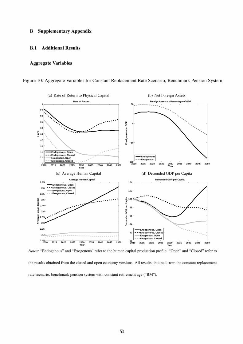
B Supplementary Appendix
B.1 Additional Results
Aggregate Variables
Figure 10: Aggregate Variables for Constant Replacement Rate Scenario, Benchmark Pension System
(a) Rate of Return to Physical Capital
2010 2015 2020 2025 2030 2035 2040 2045 20507
7.1
7.2
7.3
7.4
7.5
7.6
7.7
7.8
7.9
8
Year
r in
%
Rate of Return
Endogenous, OpenEndogenous, ClosedExogenous, OpenExogenous, Closed
(b) Net Foreign Assets
2010 2015 2020 2025 2030 2035 2040 2045 2050−100
−50
0
50
Year
For
eign
Ass
ets
/ GD
P
Foreign Assets as Percentage of GDP
EndogenousExogenous
(c) Average Human Capital
2010 2015 2020 2025 2030 2035 2040 2045 20502.15
2.2
2.25
2.3
2.35
2.4
2.45
2.5
2.55
2.6
2.65
Year
Ave
rag
e H
um
an C
apit
al
Average Human Capital
Endogenous, OpenEndogenous, ClosedExogenous, OpenExogenous, Closed
(d) Detrended GDP per Capita
2010 2015 2020 2025 2030 2035 2040 2045 205090
92
94
96
98
100
102
104
Year
Det
ren
ded
GD
P p
er C
apit
a
Detrended GDP per Capita
Endogenous, OpenEndogenous, ClosedExogenous, OpenExogenous, Closed
Notes: “Endogenous” and “Exogenous” refer to the human capital production profile. “Open” and “Closed” refer to
the results obtained from the closed and open economy versions. All results obtained from the constant replacement
rate scenario, benchmark pension system with constant retirement age (“BM”).
50
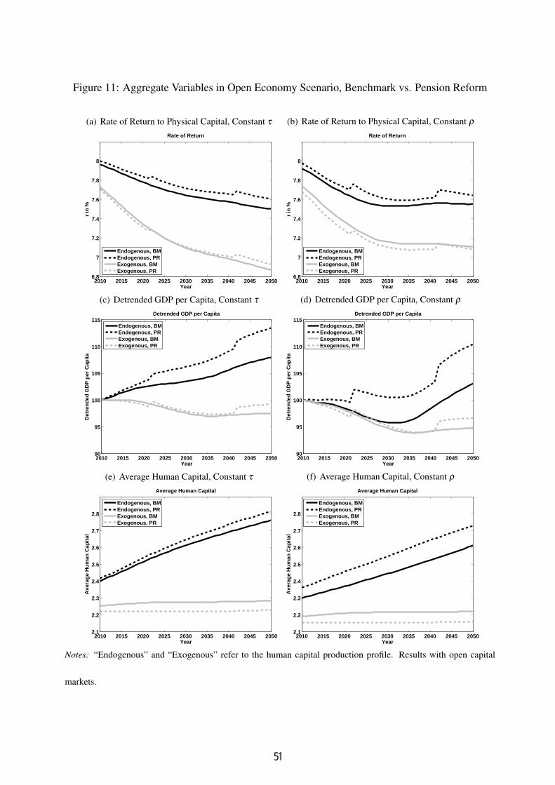
Figure 11: Aggregate Variables in Open Economy Scenario, Benchmark vs. Pension Reform
(a) Rate of Return to Physical Capital, Constant τ
2010 2015 2020 2025 2030 2035 2040 2045 20506.8
7
7.2
7.4
7.6
7.8
8
Year
r in
%
Rate of Return
Endogenous, BMEndogenous, PRExogenous, BMExogenous, PR
(b) Rate of Return to Physical Capital, Constant ρ
2010 2015 2020 2025 2030 2035 2040 2045 20506.8
7
7.2
7.4
7.6
7.8
8
Yearr
in %
Rate of Return
Endogenous, BMEndogenous, PRExogenous, BMExogenous, PR
(c) Detrended GDP per Capita, Constant τ
2010 2015 2020 2025 2030 2035 2040 2045 205090
95
100
105
110
115
Year
Det
ren
ded
GD
P p
er C
apit
a
Detrended GDP per Capita
Endogenous, BMEndogenous, PRExogenous, BMExogenous, PR
(d) Detrended GDP per Capita, Constant ρ
2010 2015 2020 2025 2030 2035 2040 2045 205090
95
100
105
110
115
Year
Det
ren
ded
GD
P p
er C
apit
a
Detrended GDP per Capita
Endogenous, BMEndogenous, PRExogenous, BMExogenous, PR
(e) Average Human Capital, Constant τ
2010 2015 2020 2025 2030 2035 2040 2045 20502.1
2.2
2.3
2.4
2.5
2.6
2.7
2.8
Year
Ave
rag
e H
um
an C
apit
al
Average Human Capital
Endogenous, BMEndogenous, PRExogenous, BMExogenous, PR
(f) Average Human Capital, Constant ρ
2010 2015 2020 2025 2030 2035 2040 2045 20502.1
2.2
2.3
2.4
2.5
2.6
2.7
2.8
Year
Ave
rag
e H
um
an C
apit
al
Average Human Capital
Endogenous, BMEndogenous, PRExogenous, BMExogenous, PR
Notes: “Endogenous” and “Exogenous” refer to the human capital production profile. Results with open capital
markets.
51

Welfare of Generations Alive in 2010 (Benchmark Model & Pension Reform)
Figure 12: Consumption Equivalent Variation of Agents alive in 2010, Benchmark Pension System
(a) Constant Replacement Rate
10 20 30 40 50 60 70 80 90−4
−3.5
−3
−2.5
−2
−1.5
−1
−0.5
0
0.5
Age
CE
V
Consumption Equivalent Variation − Cohorts alive in 2010
Endogenous, OpenEndogenous, ClosedExogenous, OpenExogenous, Closed
(b) Constant Contribution rate
10 20 30 40 50 60 70 80 90−7
−6
−5
−4
−3
−2
−1
0
1
Age
CE
V
Consumption Equivalent Variation − Cohorts alive in 2010
Endogenous, OpenEndogenous, ClosedExogenous, OpenExogenous, Closed
Notes: “Endogenous” and “Exogenous” refer to the human capital production profile. “Open” and “Closed” refer to
the results obtained from the closed and open economy versions.
Figure 13: Consumption Equivalent Variation of Agents alive in 2010, Pension Reform
(a) Constant Replacement Rate
20 30 40 50 60 70 80 90−4
−3.5
−3
−2.5
−2
−1.5
−1
−0.5
0
0.5
1
Age
CE
V
Consumption Equivalent Variation − Cohorts alive in 2010
Endogenous, BMEndogenous, PRExogenous, BMExogenous, PR
(b) Constant Contribution Rate
20 30 40 50 60 70 80 90−7
−6
−5
−4
−3
−2
−1
0
1
2
Age
CE
V
Consumption Equivalent Variation − Cohorts alive in 2010
Endogenous, BMEndogenous, PRExogenous, BMExogenous, PR
Notes: “Endogenous” and “Exogenous” refer to the human capital production profile. Results with open capital
markets.
52

Welfare of Future Generations (Benchmark Model & Pension Reform)
Figure 14: Consumption Equivalent Variation of Agents born 2010-2050, Benchmark Pension System
(a) Constant Replacement Rate
2010 2015 2020 2025 2030 2035 2040 2045 2050−8
−7
−6
−5
−4
−3
−2
Year
CE
V
Consumption Equivalent Variation − Cohorts born in 2010−2050
Endogenous, OpenEndogenous, ClosedExogenous, OpenExogenous, Closed
(b) Constant Contribution rate
2010 2015 2020 2025 2030 2035 2040 2045 20500
0.5
1
1.5
2
2.5
Year
CE
V
Consumption Equivalent Variation − Cohorts born in 2010−2050
Endogenous, OpenEndogenous, ClosedExogenous, OpenExogenous, Closed
Notes: “Endogenous” and “Exogenous” refer to the human capital production profile. “Open” and “Closed” refer
to the results obtained from the closed and open economy versions. “BM” denotes the benchmark pension system
(constant retirement age), and “PR” denotes the pension reform (increase in the retirement age).
Figure 15: Consumption Equivalent Variation of Agents born 2010-2050, Pension Reform
(a) Constant Replacement Rate
2010 2015 2020 2025 2030 2035 2040 2045 2050−6.5
−6
−5.5
−5
−4.5
−4
−3.5
−3
−2.5
−2
−1.5
Year
CE
V
Consumption Equivalent Variation − Cohorts born in 2010−2050
Endogenous, BMEndogenous, PRExogenous, BMExogenous, PR
(b) Constant Contribution Rate
2010 2015 2020 2025 2030 2035 2040 2045 20500
0.5
1
1.5
2
2.5
3
3.5
Year
CE
V
Consumption Equivalent Variation − Cohorts born in 2010−2050
Endogenous, BMEndogenous, PRExogenous, BMExogenous, PR
Notes: “Endogenous” and “Exogenous” refer to the human capital production profile. Results with open capital
markets.
53

Welfare in Closed and Open Economy
Table 5: Welfare Gains / Losses - Newborns 2010
Open EconomyPension System Constant τ Constant ρ
Endog. Exog. Endog. Exog.BM 0.8% 0.3% -3.0% -3.2%PR 1.2% 0.6% -1.7% -2.3%
Closed EconomyPension System Constant τ Constant ρ
Endog. Exog. Endog. Exog.BM 0.7% 0.3% -2.8% -3.1%PR 0.9% 0.7% -1.8% -2.1%
Notes: “Endog.” and “Exog.” refer to the endogenous and exogenous human capital production profile. “Open” and“Closed” refer to the results obtained from the closed and open economy versions. “BM” denotes the benchmarkpension system (constant retirement age), and “PR” denotes the pension reform (increase in the retirement age).
54

Table 6: Maximum Welfare Losses - Agents alive 2010
Open EconomyPension System Constant τ Constant ρ
Endog. Exog. Endog. Exog.BM -4.4% -6.5% -3.0% -3.6%PR -3.6% -6.0% -1.9% -3.0%
Closed EconomyPension System Constant τ Constant ρ
Endog. Exog. Endog. Exog.BM -4.3% -6.4% -2.8% -3.1%PR -3.6% -5.5% -1.8% -2.5%
Notes: “Endog.” and “Exog.” refer to the endogenous and exogenous human capital production profile. “Open” and“Closed” refer to the results obtained from the closed and open economy versions. “BM” denotes the benchmarkpension system (constant retirement age), and “PR” denotes the pension reform (increase in the retirement age).
55

B.2 Simple Model: Reallocation of Time over the Life Cycle
We want to understand theoretically the effects on labor supply and human capital at the inten-sive and extensive margin. We further decompose household’s reaction when we keep pricesand policy instruments fixed — i.e., wages, interest rates, the contribution rate and pensionpayments — and when we allow for general equilibrium feedback.
To understand the mechanisms theoretically, consider a simplified two-period version of themodel used in the quantitative part. Households maximize utility
U = ϕ ln(c1)+(1−ϕ) ln(1− ℓ1)+β (ϕ ln(c2)+(1−ϕ)1 ln(1− ℓ2))
s.t.
c1 +c2
1+ r= w1ℓ1(1− e)+
11+ r
(w2ℓ2h(e)1+(1−1)p)
with standard notation. h(e)≥ 1 is a strictly concave human capital production function wheree is time investment which has to be made in the first period. 1 is an indicator function takingon the value of 1 if the agent is working in the last (second) period and 0 if he is retired andreceives a pension p. Hence, changing the value of the indicator function from 0 to 1 mimicsthe pension reform of the quantitative model in a consistent way. Without loss of generality wenormalize w1 = 1. Denote first-period labor supply in the benchmark model — where 1= 0 —by ℓBM
1 and labor supply with the higher retirement age — where 1 = 1 — by ℓPR1 . Then, the
difference in labor supply after increasing the retirement age is
ℓPR1 − ℓBM
1 =β (1−ϕ)2
(1+β )(1+βϕ)− 1−ϕ
R(1+β )
(w2
h(e∗)1− e∗
− p1+β
1+βϕ
)(29)
with e∗ being the equilibrium investment into human capital. This means that — keeping humancapital constant — increasing the retirement age can in general either increase or decrease laborsupply in the first period. Labor supply in the first period increases if
β (1−ϕ)(1+βϕ)
>1R
(w2
h(e∗)1− e∗
− p1+β
1+βϕ
)whereby the right-hand-side of this condition can be interpreted as reflecting the (adjusted) dif-ference between human capital wealth — i.e., the discounted value of future income — betweenthe model without retirement — in term w2
h(e∗)1−e∗ — and with retirement — in term p 1+β
1+βϕ . If
future wages are relatively small, i.e., if w2h(e∗)1−e∗ < p 1+β
1+βϕ , then the discounted value of futureincome in case of the reform is small such that labor supply in the first period increases. Effectsare however ambiguous if future labor income is sufficiently high. An unambiguous finding isthat allowing for endogenous human capital increases h(e∗)
1−e∗ and therefore decreases labor supplywhen the retirement age increases.
56