WORKING PAPER SERIESNO 1426 / MARch 2012

cISS – A cOMPOSItE INdIcAtOR Of SyStEMIc StRESS

IN thE fINANcIAl SyStEM

by Dániel Holló, Manfred Kremer and Marco Lo Duca

NOTE: This Working Paper should not be reported as representing the views of the European Central Bank (ECB). The views expressed are

those of the authors and do not necessarily reflect those of the ECB.

MAcROPRudENtIAl RESEARch NEtWORK

© European Central Bank, 2012

Address Kaiserstrasse 29, 60311 Frankfurt am Main, GermanyPostal address Postfach 16 03 19, 60066 Frankfurt am Main, GermanyTelephone +49 69 1344 0Internet http://www.ecb.europa.euFax +49 69 1344 6000

All rights reserved.

ISSN 1725-2806 (online)

Any reproduction, publication and reprint in the form of a different publication, whether printed or produced electronically, in whole or in part, is permitted only with the explicit written authorisation of the ECB or the authors.

This paper can be downloaded without charge from http://www.ecb.europa.eu or from the Social Science Research Network elec-tronic library at http://ssrn.com/abstract_id=1611717.

Information on all of the papers published in the ECB Working Paper Series can be found on the ECB’s website, http://www.ecb.europa.eu/pub/scientific/wps/date/html/index.en.html

Macroprudential Research NetworkThis paper presents research conducted within the Macroprudential Research Network (MaRs). The network is composed of econo-mists from the European System of Central Banks (ESCB), i.e. the 27 national central banks of the European Union (EU) and the European Central Bank. The objective of MaRs is to develop core conceptual frameworks, models and/or tools supporting macro-prudential supervision in the EU.

The research is carried out in three work streams: 1) Macro-financial models linking financial stability and the performance of the economy; 2) Early warning systems and systemic risk indicators; 3) Assessing contagion risks.

MaRs is chaired by Philipp Hartmann (ECB). Paolo Angelini (Banca d’Italia), Laurent Clerc (Banque de France), Carsten Detken (ECB) and Katerina Šmídková (Czech National Bank) are workstream coordinators. Xavier Freixas (Universitat Pompeu Fabra) acts as external consultant and Angela Maddaloni (ECB) as Secretary.

The refereeing process of this paper has been coordinated by a team composed of Cornelia Holthausen, Kalin Nikolov and Bernd Schwaab (all ECB).

The paper is released in order to make the research of MaRs generally available, in preliminary form, to encourage comments and suggestions prior to final publication. The views expressed in the paper are the ones of the author(s) and do not necessarily reflect those of the ECB or of the ESCB.

AcknowledgementsWe thank Philipp Hartmann for inspiring and supporting this project throughout all stages. Philipp also invented the indicator’s name and its abbreviation CISS (pronounced like “kiss”). We thank Tommy Kostka for excellent research assistance and for several good ideas which helped improving the CISS. Very helpful comments from Geert Bekaert, Wolfgang Lemke, Simone Manganelli and an anonymous referee are gratefully acknowledged. We finally thank participants at the Euro Area Business Cycle Network conference “Econometric Modelling of Macro-Financial Linkages” in Florence and the 5th CSDA International Conference on Computational and Financial Econometrics in London for fruitful discussions and comments. However, the views expressed in this paper are those of the authors and do not necessarily reflect those of the European Central Bank, the Eurosystem or the Magyar Nemzeti Bank.

CISS indicatorPlease find weekly updates of the CISS data here.

Dániel Hollóat Magyar Nemzeti Bank, 1054 Szabadság tér 8/9, 1850 Budapest, Hungary; e-mail: hollod@mnb.hu

Manfred Kremer (corresponding author)at European Central Bank, Kaiserstrasse 29, D-60311 Frankfurt am Main, Germany; e-mail: manfred.kremer@ecb.europa.eu

Marco Lo Ducaat European Central Bank, Kaiserstrasse 29, D-60311 Frankfurt am Main, Germany; e-mail: marco.lo_duca@ecb.europa.eu

Abstract

This paper introduces a new indicator of contemporaneous stress in the financial system named

Composite Indicator of Systemic Stress (CISS). Its specific statistical design is shaped according to

standard definitions of systemic risk. The main methodological innovation of the CISS is the application

of basic portfolio theory to the aggregation of five market-specific subindices created from a total of 15

individual financial stress measures. The aggregation accordingly takes into account the time-varying

cross-correlations between the subindices. As a result, the CISS puts relatively more weight on situations

in which stress prevails in several market segments at the same time, capturing the idea that financial

stress is more systemic and thus more dangerous for the economy as a whole if financial instability

spreads more widely across the whole financial system. Applied to euro area data, we determine within a

threshold VAR model a systemic crisis-level of the CISS at which financial stress tends to depress real

economic activity.

Keywords: Financial system, Financial stability, Systemic risk, Financial stress index, Macro-financial

linkages

JEL Classifications: G01, G10, G20, E44

1

Non-technical Summary

The recent financial and economic crisis revealed considerable gaps in the theoretical and empirical

frameworks for analysing, monitoring and controlling systemic risk in the financial system. Academics

and financial authorities all around the globe accordingly have been stepping up their efforts to improve

the suit of tools and models in the field of systemic risk and macroprudential analysis, respectively. This

paper contributes to the empirical branch of this strand of literature by introducing a new indicator of

contemporaneous instability or “stress” in the financial system. The proposed indicator is named

Composite Indicator of Systemic Stress or simply CISS (pronounced “KISS”). The main general goal of

using stress indices such as the CISS is to measure the current state of instability, i.e. the current level of

frictions, stresses and strains (or the absence of these) in the financial system and to condense that state of

financial instability into a single statistic. The specific aim of the CISS is to emphasise the systemic

nature of existing stresses in the financial system, where systemic stress is interpreted as an ex post

measure of systemic risk, i.e. risk which has materialised already. The CISS permits not only the real time

monitoring and assessment of the stress level in the whole financial system, but may also help delineating

historical episodes of “financial crises” which might then be better compared and studied empirically in

the context of early warning signal models, for instance. Last but not least, composite financial stress

indicators can also be used to gauge the impact of policy measures directed towards mitigating systemic

stress.

The main strength of the CISS compared to alternative financial stress indicators is its explicit conceptual

foundation on standard definitions of systemic risk and the adoption of a statistical measurement

framework suitable to capture some of the main symptoms characterising systemic crises. The CISS

comprises the five arguably most important segments of an economy’s financial system: the sector of

bank and non-bank financial intermediaries, money markets, securities (equities and bonds) markets as

well as foreign exchange markets. The current level of stress in each of these five segments is measured

on the basis of three raw stress indicators capturing certain symptoms of financial stress such as increases

in agents’ uncertainty, investor disagreement or information asymmetries. Certain raw stress indicators

shall also capture flight-to-quality and flight-to-liquidity effects, respectively. The CISS measures such

stress symptoms mainly on the basis of securities market indicators which are quite standard in the

literature (such as volatilities, risk spreads and cumulative valuation losses). These indicators are readily

available for many countries at a daily frequency in general and with relatively long data histories. The

CISS can accordingly be updated more or less in real time and computed for a relatively broad set of

countries stretching even beyond the major developed economies.

The main methodological innovation of the CISS is the application of standard portfolio theory to the

aggregation of the five segment-specific stress measures into the composite indicator. Precisely, the sub-

indices are aggregated on the basis of weights which reflect their time-varying cross-correlation structure.

2

As a result, the CISS puts relatively more weight on situations in which stress prevails in several market

segments at the same time. This is why we claim the CISS to be a more appropriate measure of systemic

stress. Two differentiating features of the CISS are its targeted robustness to the arrival of new

information – mainly achieved by the specific quantiles-based transformation of raw stress indicators -

and its recursive (“real time”) computation over expanding samples.

An evaluation of the CISS applied to euro area data confirms its robustness over time such that it largely

avoids the problem of regime/event reclassification. In addition, the euro area CISS appears to peak

during well-known periods of elevated financial stress, but it also singles out the recent economic and

financial crisis as a unique event in terms of the levels of stress observed in the full data sample available

(starting in 1987). In contrast, if the CISS is calculated as a simple arithmetic average - which implicitly

assumes perfect correlation across all sub-indices all the times - it would not be able to differentiate so

clearly between the system-wide levels of stress prevailing for example, in the aftermath of September 11,

2001 and during several stages of the recent global financial and economic crisis. Hence, indicators not

incorporating the systemic nature of stress might provide misleading information regarding the “true

levels” of strains and imbalances in the financial system.

We also propose new ways to determine critical levels (i.e., crisis thresholds and regimes) for composite

financial stress indices as the endogenous outcome of two variants of parsimonious econometric regime-

switching models. The basic idea behind both modelling approaches is that the dynamics of the financial

system and its interactions with the real sector may be subject to multiple equilibria depending on

whether the economy is in a state of financial crises and non-crises, respectively. This may reflect the fact

that the interaction between externalities (e.g., contagion), information problems (e.g., phenomena related

to asymmetric information such as adverse selection) and certain special features of the financial sector

(e.g., the existence of illiquid assets, maturity mismatches, leverage) can lead to powerful feedback and

amplification mechanisms driving the system from a state of relative tranquillity to a state of turmoil, also

altering the system’s normal laws of motion. The first approach consists of an autoregressive Markov-

switching model that tries to capture such “phase transitions” by modelling the dynamics of the CISS

itself. The second econometric approach tries to capture such regime shifts by assessing the interaction of

the CISS with a measure of real economic activity. The approach comprises a threshold vector

autoregression model which identifies on statistical grounds a critical level of the CISS (the threshold

value) at or above which financial stress exerts a very strong negative impact on economic activity, while

no significant relationship can be found for periods when the CISS stands below that threshold.

It should be borne in mind, however, that the CISS can only provide a very rough, stylised and highly

imperfect view on the state of instability in a real-world financial system given its nature as a necessarily

very imperfect composite indicator on the one hand, and the complex, multifaceted and elusive nature of

systemic risk as well as severe data limitations on the other hand.

3

1. Introduction

The financial and economic crisis still ongoing at the time of writing, started with growing strains in the

US subprime mortgage market. In August 2007 BNP Paribas was forced to halt redemptions on three of

its investment funds with large exposures to securitisation assets backed by US subprime mortgages

which had become largely illiquid. This was the moment when local strains in one particular US asset

market triggered a truly “systemic event” in large parts of the global financial system. The crisis further

intensified in September 2008 in reaction to the failure of Lehman Brothers. This event clearly shifted the

crisis into a higher gear with financial frictions starting to have serious adverse impacts on the global

economy which, in turn, further aggravated the level of strains in the financial system. This vicious cycle

deepened further and widened the scope of the crisis in terms of its geographical coverage and the breadth

of affected market segments. For example, the crisis now also spilled over into many emerging markets

and eventually brought about the sovereign crisis in Europe in early 2010. In general, the levels of

tensions in the global and local financial systems varied over time, with catalytic events triggering new

stress peaks and subsequent periods of gradual and partial recovery and so forth.

While it makes sense to associate financial crises episodes to its main identifying events, a sufficient

characterisation of a particular crisis requires more systematic and quantified information. For example,

while the start of a crisis can be typically traced to a specific triggering event, its end point is usually left

open. The focus on events neither lends itself to a quantification of the stress levels reached at different

stages of a particular episode. In addition, although each financial crisis in a country’s history is unique in

its root causes, its propagating channels and market segments ultimately affected, it may still be

interesting to make these different events comparable along the dimension of the overall systemic stress

levels reached.

In order to address some of these issues, this paper introduces a new financial stress index called

“Composite Indicator of Systemic Stress” or simply “CISS”. The main general aim of financial stress

indices (FSIs) such as the CISS is to measure the current state of instability, i.e. the current level of

frictions, stresses and strains (or the absence thereof) in the financial system and to summarise it in a

single (usually continuous) statistic. While it would be unrealistic to expect that such a highly condensed

composite index can sufficiently characterise something as complex as systemic risk (Billio et al. 2011),

FSIs still have their merits. A comprehensive FSI not only permits the real time monitoring and

4

assessment of the stress level in the whole financial system, but it may also help to better delineate and

describe historical crisis episodes. FSIs may furthermore improve the statistical power and the

information content of macroprudential early warning signal models which typically use binary crisis

variables as dependent variables (see Illing and Liu 2006, and recent applications by Misina and Tkacz

2009 and Lo Duca and Peltonen 2011). Moreover, FSIs might also be used to gauge the impact of policy

measures aimed at alleviating financial instability.

The main distinguishing feature of the CISS vis-à-vis alternative FSIs is its focus on the systemic

dimension of financial stress. This is achieved by a specific statistical design which is shaped according to

standard definitions of systemic risk. The CISS comprises 15 mostly market-based financial stress

measures equally split into five categories, namely the financial intermediaries sector, money markets,

equity markets, bond markets and foreign exchange markets, arguably representing the most important

segments of an economy’s financial system. A separate financial stress subindex is computed for each of

these five market segments after appropriate transformation of the individual stress measures. The main

methodological innovation of the CISS is the application of basic portfolio theory to the aggregation of

the subindices into the composite indicator. The portfolio-theoretic aggregation takes into account the

time-varying cross-correlations between the subindices. As a result, the CISS puts relatively more weight

on situations in which stress prevails in several market segments at the same time which, in turn, captures

the idea that systemic risk/stress is high if financial instability is spread widely across the whole financial

system. The second element of the aggregation scheme featuring systemic risk, is the fact that the

“portfolio weights” attached to each of the five subindices are calibrated on the basis of the relative

strength of their dynamic impact on a measure of economic activity (“real-impact weights”). Two further

differentiating features of the CISS are its targeted robustness to the arrival of new information – mainly

achieved by transforming the raw stress indicators into order statistics from their empirical cumulative

distribution function (CDF) - and its recursive (“real time”) computation over expanding samples. Both

features shall mitigate the potential problem of regime/event reclassification which may affect in

particular those financial stress indicators whose statistical design relies strongly on stable distribution

properties of the underlying data in typically small samples.

Many alternative FSIs have been developed recently, in most cases in response to analytical demands

generated by the financial crisis. The following literature review is not exhaustive but focussed on

illustrating the broad range of existing methodologies and the country coverage. Illing and Liu (2006) is a

seminal paper in this strand of literature. They developed a daily financial stress index for the Canadian

financial system and proposed several approaches to the aggregation of individual stress indicators into a

composite stress index. Their preferred FSI-specification was chosen according to which variant performs

best in capturing crisis events in the Canadian financial system identified on the basis of a survey among

Bank of Canada policy-makers and staff. Their FSI comprises eleven financial market variables which are

aggregated on the basis of weights determined by the relative size of the market to which each of the

indicators pertain compared to a broad measure of total credit in the economy. Caldarelli, Elekdag and

5

Lall (2011) present a monthly financial stress index for 17 advanced economies computed as the

arithmetic average of twelve standardised market-based financial stress indicators, an aggregation method

also known as “variance-equal weighting”. While the individual indicators in that study are grouped into

three subindices - which can be thought of being associated with the banking, securities, and foreign

exchange markets -, the grouping itself is irrelevant for the computation of the composite indicator. The

same approach has been taken by Yiu, Ho and Jin (2010) in computing a monthly FSI for Hong Kong

with six financial market input series. The ECB (2009a) develops a “Global Index of Financial

Turbulence” (GIFT) from parsimonious stress indicators for 29 main economies each comprising six

market-based indicators - capturing stress in fixed income, equity and foreign exchange markets – which

are also variance-equal weighted and subsequently normalised by logistical transformation. Lo Duca and

Peltonen (2011) produced parsimonious FSIs for 10 advanced and 18 emerging economies by taking the

arithmetic average of five raw stress indicators, each transformed on the basis of its quartiles derived from

the empirical CDF.

Nelson and Perli (2007) at the Federal Reserve Board present a weekly “financial fragility indicator” for

the United States computed in two steps from twelve market-based financial stress measures. The

standardised input series are first reduced to three summary indicators, namely the level factor (the

variance-equal weighted average), the rate-of-change factor (rolling eight-week percentage change in the

level factor) and the correlation factor (percentage of total variation in the individual stress variables

explained by the first principal component over a rolling 26-week window). In the second step, the

financial fragility indicator is computed as the fitted probability from a logit model with the three

summary indicators as explanatory variables and a binary pre-defined crisis indicator as the dependent

variable. Following the approach by Nelson and Perli (2007), Blix Grimaldi (2010) computes a similar

weekly FSI for the euro area based on 16 financial market variables, whereby only the level and the rate-

of-change factor enter the probit regression as explanatory variables (the correlation factor does not turn

out statistically significant); crisis events for the computation of the binary indicator are identified on the

basis of a keyword-search through relevant parts of the ECB Monthly Bulletin.

Building on eleven daily financial market indicators as input series, Hakkio and Keeton (2009) at the

Federal Reserve Bank of Kansas City construct a monthly FSI (the “KCFSI”) applying principal

components analysis to US data. The idea is that financial stress is the factor most responsible for the

observed correlation between the indicators, and this factor is identified by the first principal component

(the first eigenvalue) of the sample correlation matrix computed for the standardised indicators. The

weights with which each individual indicator enters into the composite FSI are computed from the

indicators’ loadings to the first principal component, i.e. from the first eigenvector of the correlation

matrix. Applying the same methodology, Kliesen and Smith (2010) aggregate 18 weekly financial market

indicators into the “St. Louis Fed’s Financial Stress Index” (STLFSI). The weekly “financial conditions

index” (FCI) developed by Brave and Butters (2011a, 2011b) also builds on factor analysis but is more

complex and sophisticated than its competitors in terms of the number and the heterogeneity of the input

6

data and the statistical indicator design. The computation of the FCI is cast into a dynamic factor model in

state-space form which includes 100 indicators capturing conditions in money markets, debt and equity

markets, as well as in the banking system. The model, and thus the FCI, is estimated by a specific variant

of the EM algorithm, where Kalman filtering takes account of the missing data problem resulting from the

different sample lengths and frequencies of the input data. Van Roye (2011) pursues an approach similar

to the one by Brave and Butters (2011a) to construct a “financial market stress indicator” (FSMI) for

Germany and the euro area. The German and euro area indicators comprise 23 and 22 raw stress factors

covering the banking sector, securities markets and foreign exchange conditions.

The “Cleveland Financial Stress Index” (CFSI) developed by Oet et al. (2011) integrates 11 daily

financial market indicators which are grouped into four sectors (debt, equity, foreign exchange and

banking markets). The raw indicators are normalised by transforming the values of each series into the

corresponding value of their empirical CDF. The transformation method is basically identical to the one

developed independently in the present paper. The transformed indicators are then aggregated into the

composite indicator by applying time-varying credit weights which are proportional to the quarterly

financing flows through the four markets concerned. As in Illing and Liu (2006), the CFSI with credit

weights emerges as the preferred specification compared to alternative weighting schemes. Inspired by an

earlier version of the present paper, Louzis and Vouldis (2011) construct a monthly “Financial Systemic

Stress Index” for Greece where five subindices are aggregated based on portfolio-theoretic principles, i.e.

by taking into account their cross-correlations here estimated by a multivariate GARCH model. The

subindices comprise 14 individual stress measures derived from financial market data but also from

monthly bank balance sheet data. Principal component analysis is applied at the subindex level, and the

subindices are normalised using logistical transformation.

An evaluation of the CISS applied to euro area data confirms its robustness over time, ruling out

problems associated with ex post reclassifications of crisis events. Furthermore, the euro area CISS

appears to peak during well-known periods of elevated financial stress, and it singles out the recent

economic and financial crisis as a unique event in terms of the levels of stress observed in the data sample

available. In contrast, if the CISS is calculated as a simple arithmetic average of the five subindices -

which implicitly assumes perfect correlation across all subindices at all the times - it would not be able to

differentiate so clearly between the systemic levels of stress prevailing, for example, in the aftermath of

September 11, 2001 and several stages of the recent global financial and economic crisis. Hence,

indicators not incorporating the “systemic” nature of stress might underestimate the “true” levels of

strains and imbalances in the financial system. We moreover present two parsimonious econometric

approaches to endogenously identify different financial stress regimes. The first is an autoregressive

Markov-switching model that tries to capture such regime shifts by modelling the dynamics of the CISS

itself. The second approach consists of a threshold vector autoregression (TVAR) model which

determines a level of the CISS at which systemic financial stress becomes so severe that it substantially

impairs real economic activity. The results from the TVAR indeed suggest that the real effects of

7

financial stress differ dramatically between the low and the high stress regimes. While shocks in the CISS

do not exert any statistically significant output reactions during low-stress regimes, industrial production

truly collapses during high-stress regimes. Similarly, it is only during high stress regimes that for instance

a negative output shock leads to a subsequent increase in financial stress. Taken together, these mutual

reaction patterns seem to confirm the idea that when hit by a sufficiently large shock an economy faces

the risk of entering a vicious downward spiral with financial and economic stress reinforcing each other

over time, a finding which could be explained theoretically by some financial accelerator mechanism

(see, e.g., Bernanke, Gertler and Gilchrist 1999). The regime-dependence of the impact of financial stress

on economic activity broadly corroborates the findings of Davig and Hakkio (2010) from a bivariate

Markov-switching model with the above-mentioned KCFSI and a monthly measure of US economic

activity as endogenous variables. Hubrich and Tetlow (2011) for the US and Hartmann et al. (2012) for

the euro area provide qualitatively similar evidence on stronger impacts of financial stress on economic

activity in high-stress regimes within richer specifications of Markov-switching VARs, where the latter

study uses the CISS to measure financial stress. The present paper therefore also relates to the general

literature examining empirically the real impacts of financial stress (e.g., Hakkio and Keeton 2009,

Cardarelli, Elekdag and Lall (2011), Hatzius et al. 2010, Li and St-Amant 2010, Mallick and Sousa 2011,

Carlson, King and Lewis 2011, and van Roye 2011).

The remainder of this paper is organised as follows: Section 2 offers some theoretical considerations

motivating the specific statistical design of the CISS which rests on standard definitions of systemic risk.

Section 3 describes the statistical design of the indicator based on data for the euro area as a whole. The

euro area CISS is evaluated in Section 4 in terms of its robustness properties and its ability to identify

well-known periods of financial stress. This section also presents results from the two econometric

approaches applied to determine different regimes in the CISS. Section 5 concludes.

2. Theoretical background: Systemic risk and symptoms of financial stress

The CISS aims to measure the current state of instability in the financial system as a whole or,

equivalently, the level of “systemic stress”. Systemic stress is interpreted as that amount of systemic risk

which has already materialised. Systemic risk, in turn, can be defined as the risk that financial instability

becomes so widespread that it impairs the functioning of a financial system to the point where economic

growth and welfare suffer materially (de Bandt and Hartmann 2000, de Bandt, Hartmann and Peydro

2009, ECB 2009b).1 It distinguishes “(…) between a ‘horizontal’ perspective of systemic risk, where

attention is confined to the financial system, and a ‘vertical’ perspective of systemic risk in which the two-

sided interaction between the financial system and the economy at large is taken into account as well.

1 In substance similar definitions of systemic risk have become standard also in international policy circles, with the following definition as an example: “The paper defines systemic risk as a risk of disruption to financial services that is (i) caused by an impairment of all or parts of the financial system and (ii) has the potential to have serious negative consequences for the real economy” (IMF-BIS-FSB 2009).

8

Ideally, the severity of systemic risk and systemic events would be assessed by means of the effect that

they have on consumption, investment and growth or economic welfare broadly speaking” (ECB 2009b).

Against this background, the CISS shall be designed in a way such that it both operationalises the idea of

widespread financial instability (horizontal view) and captures the importance of financial stress for the

real economy (vertical view). Both requirements can be associated with the notion of systemic

importance. If the aim is to measure widespread, disruptive and economically harmful strains in the

financial system, the CISS has to capture the level of stress in its economically most important, i.e.

systemically most risky elements. Size, substitutability and interconnectedness are usually three of the

main criteria applied to identify systemically important financial institutions and markets. According to

the size criterion, the CISS comprises individual financial stress indicators which mostly reflect stability

conditions in large aggregated markets and financial sectors which collectively represent the core of any

financial system (see Sections 3.1 and 3.2). In addition, the markets and sectors included in the CISS are

aggregated to such an extent that in case financial stress disrupts all of them at the same time, no major

substitute forms of unimpaired finance presumably exist in the economy. The interconnectedness

criterion is not directly addressed. However, time-varying degrees of interconnectedness between the

included markets and sectors may be indirectly reflected in the proposed portfolio-theoretic aggregation

scheme for the composite indicator (see Section 3.4).

What remains to be specified is a more precise meaning of financial instability or stress itself and how it

can be measured. For this purpose, we draw on the main symptoms typically associated with crisis

situations in which the “normal functioning” of financial markets is impaired (Hakkio and Keeton 2009).

The literature suggests several key features of financial stress to be present under crisis conditions (e.g.,

Hakkio and Keeton 2009, Fostel and Geneakoplos 2008): an increase in uncertainty (e.g., concerning

asset valuations and the behaviour of other investors); an increase in disagreement (differences of

opinion) among investors; an increase in the asymmetry of information between borrowers and lenders

(intensifying problems of adverse selection and moral hazard); and a reduced preference for holding risky

assets (flight-to-quality) and/or illiquid assets (flight-to-liquidity) which may result from stronger risk or

uncertainty aversion, for instance (Caballero and Krishnamurthy 2008). These different features of

financial stress are often closely interrelated, with a tendency to reinforce each other as in the case of fire

sales and liquidity spirals, a situation in which declining market and funding liquidity exacerbate each

other (Brunnermeier 2009; Brunnermeier and Pedersen 2009; Krishnamurthy 2010). The various stress

features bring about observable symptoms of financial stress such as, inter alia, higher asset price

volatility, large asset valuation losses, as well as wider default and liquidity risk premia. Most of these

individual characteristics of financial stress can be captured more or less imperfectly by quite standard

financial market indicators (see Sections 3.2 and 3.3). It is far less clear, though, how to measure the

overall level of financial stress, which is the aim of the CISS.

9

3. Statistical design of the CISS

This section first presents the basic setup of the CISS (Section 3.1) and then compiles a set of indicators

which capture the typical symptoms of financial stress in five representative market segments on the basis

of euro area data (Section 3.2). These individual “raw stress indicators” are then standardised by means of

transformation into order statistics, and the arithmetic averages of the three transformed “stress factors” in

each submarket constitute the five subindices of financial stress (Section 3.3). These subindices are

finally aggregated into our “composite indicator of systemic stress” in an innovative manner following

portfolio-theoretical principles (Section 3.4). In our view, this novel aggregation scheme takes some of

the essential characteristics of systemic stress better into account. The section concludes with a

presentation of a backward extended version of the CISS starting in 1987, i.e. twelve years prior to the

introduction of the euro (Section 3.5).

3.1 Basic setup

Ideally, the CISS measures the level of stress in the financial system as a whole. However, a financial

system in the real world is a very complex and complicated network of financial markets, financial

intermediaries and financial infrastructures with all playing a crucial role for the stability properties of the

system. As it is practically impossible to measure the level of strains in all elements of the financial

system, it makes sense to focus on its systemically most important parts and to abstract from others. For

this purpose, we organise the selection of individual indicators for financial stress according to the

general and very basic structure for the construction of financial stress indices as sketched in Figure 1.

The financial system can be divided into three main building blocks: markets, intermediaries and

infrastructures. Each of these building blocks can be split into specific segments (e.g., the financial

intermediaries segment can be separated into different sectors like banks, insurance companies, hedge

funds etc.) which, in turn, can be further broken down into certain financial instruments, subsectors or

subinfrastructures, respectively. According to Figure 1 there principally exist three different levels at

which composite financial stress indexes can be computed from a certain set of individual “micro” stress

indicators (like a certain risk spread or asset volatility). The lower level of aggregation comprises

segment-specific stress indices which can be directly calculated by aggregating a representative set of

constituent individual stress indicators. The intermediate level is composed of stress indices for each of

the three building blocks which can, for instance, be computed by aggregating the lower-level stress

indices. Finally, the top level constitutes the composite financial stress indicator for the whole financial

system. It comprises elements from in principle all lower level building blocks and market segments.

However, due to data limitations the basic structure of none of the existing FSIs, including the CISS, is as

comprehensive as laid out in Figure 1. In particular, data limitations usually prevent computation of stress

10

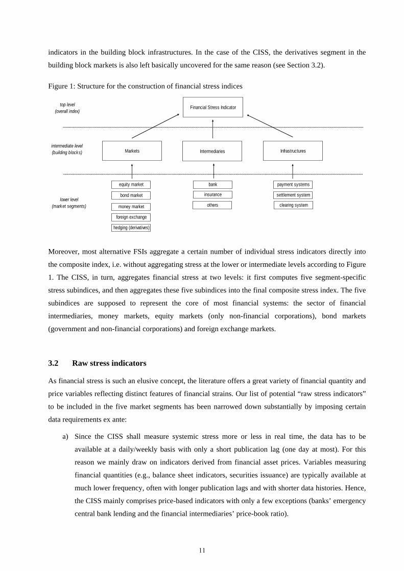
indicators in the building block infrastructures. In the case of the CISS, the derivatives segment in the

building block markets is also left basically uncovered for the same reason (see Section 3.2).

Figure 1: Structure for the construction of financial stress indices

lower level(market segments)

equity market

bond market

money market

foreign exchange

hedging (derivatives)

bank

insurance

others

payment systems

settlement system

clearing system

Markets Intermediaries Infrastructures

Financial Stress Indicatortop level(overall index)

intermediate level(building blocks)

Moreover, most alternative FSIs aggregate a certain number of individual stress indicators directly into

the composite index, i.e. without aggregating stress at the lower or intermediate levels according to Figure

1. The CISS, in turn, aggregates financial stress at two levels: it first computes five segment-specific

stress subindices, and then aggregates these five subindices into the final composite stress index. The five

subindices are supposed to represent the core of most financial systems: the sector of financial

intermediaries, money markets, equity markets (only non-financial corporations), bond markets

(government and non-financial corporations) and foreign exchange markets.

3.2 Raw stress indicators

As financial stress is such an elusive concept, the literature offers a great variety of financial quantity and

price variables reflecting distinct features of financial strains. Our list of potential “raw stress indicators”

to be included in the five market segments has been narrowed down substantially by imposing certain

data requirements ex ante:

a) Since the CISS shall measure systemic stress more or less in real time, the data has to be

available at a daily/weekly basis with only a short publication lag (one day at most). For this

reason we mainly draw on indicators derived from financial asset prices. Variables measuring

financial quantities (e.g., balance sheet indicators, securities issuance) are typically available at

much lower frequency, often with longer publication lags and with shorter data histories. Hence,

the CISS mainly comprises price-based indicators with only a few exceptions (banks’ emergency

central bank lending and the financial intermediaries’ price-book ratio).

11

b) The stress indicators should represent market-wide developments. We therefore prefer broad

market indices but sometimes also revert to certain assets with benchmark status for the pricing

of close substitutes (e.g., government bonds).

c) The CISS shall be computable for a wide range of (sufficiently developed) countries and thus

should be based on a comparable set of indicators.

d) The CISS shall be available for sufficiently long data samples such that it comprises several

episodes of financial stress as well as business cycles in the respective economies.

Requirements c) and d) imply that the CISS includes mainly standard indicators available for many

countries with relatively long data histories. This is also the reason why we have not made use of

financial derivatives prices, with the exception of interest rate swap data.2

Each subindex is furthermore restricted to include (at most) three stress indicators, such that the

composite indicator eventually comprises a total of 15 individual indicators of financial stress.3 In

principle, the three stress indicators of each subindex capture one or more of the typical symptoms of

financial stress. Moreover, the indicators should not convey identical but, to the extent possible,

complementary information about the level of strains in the same market segment. Ideally, all three

indicators in each subindex should be perfectly correlated only under severe levels of strains (such as

under totally dysfunctional market conditions), while lower levels of stress should leave some room for

differentiation across the subindex components.

We mostly rely on realised asset return volatilities (included in all five subindices) and on risk spreads to

capture the main symptoms of financial stress in the various market segments (details on the computation

and the data sources of all individual stress indicators are given in Table 1 located in Section 3.3). Asset

return volatilities tend to increase with investors’ uncertainty about future fundamentals and/or the

behaviour and sentiment of other investors. For instance, in Pastor and Veronesi (2009) volatility

increases caused by a higher “news elasticity” of asset prices when investors’ uncertainty about the

asset’s underlying fundamentals has increased. Veronesi (2004) furthermore shows that a small

probability of a long recession can induce volatility to cluster at high levels during recessions, a situation

which often occurs in the context of systemic crises. Chordia, Sarkar and Subrahmanyam (2005) present

evidence that volatility shocks in bond and stock markets tend to predict shifts in liquidity condition in

both markets, possibly explained by volatility-induced changes in the inventory risk borne by market

making agents. Apart from realised interest rate volatility, stress in the money market is also captured by

a euro area equivalent of the US TED spread, i.e. by the yield differential between a short-term

unsecured inter-bank market rate and a comparable essentially risk-free Treasury bill rate. This spread

2 Interest rate swaps have for long been a standard and very important instrument both in terms of volume and benchmark status.

12

reflects liquidity and counterparty risk in the inter-bank market (as in Heider, Hoerova and Holthausen

2010 or Acharya and Skeie 2011) as well as the convenience premium on short-term Treasury paper, and

thus captures stress features like flight-to-quality, flight-to-liquidity as well as the price impacts of

enhanced adverse selection problems in times of banking stress. Another variable measuring money

market stress is a scaled version of banks’ emergency lending at national central banks of the Eurosystem

reflecting, inter alia, strained liquidity conditions in the inter-bank market. A measure of bond market

stress is the yield spread of A-rated bonds of non-financial corporations against a comparable

government bond. This yield spread contains default and liquidity risk premia which shall capture flight-

to-quality and flight-to-liquidity phenomena, i.e., the spread should increase if investors become more

concerned about solvency issues and if liquidity conditions in the corporate bond market deteriorate, but

also in response to higher risk aversion and uncertainty.4 Drawing on the empirical findings of Feldhütter

and Lando (2009) for the US, the ten-year swap spread is arguably a relatively clean measure of the

convenience yield embedded in the prices of German government bonds – the presumably safest and

most liquid sovereign bonds in the euro area – which, in turn, captures well flight-to-liquidity and flight-

to-quality effects in this market segment.5 One measure of stress in the equity market is the so-called

CMAX measuring the maximum cumulated loss over a moving two-year window. It has originally been

developed to identify crisis periods in international stock markets (Patel and Sarkar 1998; see Coudert

and Gex 2006 for a more recent application) but is now often used as an ingredient in financial stress

indicators (e.g., Illing and Liu 2006). Stress in the equity market is furthermore measured by a time-

varying correlation coefficient between stock and government bond returns capturing, amongst others,

flight-to-liquidity and flight-to-quality phenomena (Baele, Bekaert and Inghelbrecht 2010). For instance,

in times of heightened systemic stress, investors try to shift funds out of more risky stocks into safer

government bonds, thereby driving the return correlation between these two asset classes into negative

territory. Since our stress factors shall all increase with higher levels of stress, we take the negative of the

short-term stock-bond correlation (measured as the deviation from a long-term correlation to account for

persistent correlation trends) as the stress indictor. Stress in the financial intermediaries sector is

measured by idiosyncratic stock return volatility of the banking sector and the yield differential between

A-rated financial and non-financial corporations. A partly novel stress measure of the financial

intermediaries segment is obtained by interacting the CMAX of this sector with its inverse price-book

3 The same number of indicators per subindex ensures that the subindices – which are computed as simple averages of the transformed stress factors – do not possess different statistical properties by construction. For example, if all individual stress indicators were standard normal distributed, the variance of the average of stress indicators would decrease with the number of indicators included. 4 The yield spreads of AAA-rated corporations may be an inferior measure of bond market stress compared to spreads on lower-rated bonds. Dick-Nielsen, Feldhütter and Lando (2012) have shown for the US corporate bond market that AAA-rated bonds benefited from flight-to-liquidity effects during the subprime crisis through lower liquidity premia, while the liquidity risk components in the yields spreads of corporate bonds with lower ratings went up instead. 5 On the convenience yields in US Treasuries see also Krishnamurthy and Vissing-Jorgensen 2010. Krishnamurthy (2010) describes how limits-to-arbitrage problems appeared to distort US swap spreads towards very unusual negative values during the subprime crisis, i.e. during periods of extreme stress.

13

ratio. The idea behind this indicator is that any given large stock market loss puts a financial

intermediary the more under stress the lower the current level of stock market valuation as measured for

the present purpose by the price-book ratio. Values of this ratio below one indicate that the present

market value of a corporation has fallen below its book value as it has been the case for the euro area

financial sector index since early October 2008. Financials reached their lowest valuation level during

the current crisis in March 2009, when their aggregate market value fell to a mere 40% of book values.

Stress in the foreign exchange market is exclusively represented by the realised volatility of three

bilateral euro exchange rates.

3.3 Transformation of raw indicators by means of order statistics

The aggregation of individual stress indicators is arguably the most difficult aspect of constructing

composite financial stress indicators (Illing and Liu 2006). The literature offers several options, all

coming with specific advantages and disadvantages. In most cases aggregation starts with putting the

individual raw stress indicators on a common scale by standardisation, i.e. by subtracting the sample

mean from the raw score and dividing this difference by the sample standard deviation. The standardised

indicators are then usually aggregated into a composite indicator by either taking their arithmetic average

(“variance-equal weighting”) or by applying principal components analysis. Standardisation, however,

implicitly assumes variables to be normally distributed. The fact that many standard stress indicators

clearly violate this assumption (e.g., in the case of variances) enhances the risk that the results obtained

from the use of standardised variables are sensitive to aberrant observations. In that case, for instance,

both the conditional means and the standard deviations - when calculated over expanding data samples -

can be subject to large revisions if more and more outliers are added to the sample (Hakkio and Keeton

2009) as it tends to happen in particular during extended periods of severe financial stress. Such problems

can distort the information content of financial stress indicators over time (see the general discussion of

the event reclassification problem in Section 4.1).6

We therefore put much emphasis from the outset on the robustness properties of our composite indicator

in the time dimension. In general, the problem of robustness as just described can be mitigated by

transforming the raw stress indicators on the basis of location and dispersion measures of their empirical

distribution function which are more robust than the mean and the standard deviation (see Stuart and Ord

1994). We instead propose a transformation of raw stress indicators based on their empirical cumulative

distribution function (CDF) involving the computation of order statistics.

Let us denote a particular data set of a raw stress indicator xt as ),,,( 21 nxxxx with n the total

number of observations in the sample. The ordered sample is denoted where ), ][nx,,( ]2[]1[ xx

14

][]2[]1[ nxxx and [r] referred to as the ranking number assigned to a particular realisation of xt.

All values of the original data set are arranged in ascending order such that the order statistic x[n]

represents the sample maximum, i.e. the highest level of a stress indicator in a given sample, and x[1]

accordingly the sample minimum. The transformed stress indicators (the stress factors) zt are now

computed from the raw stress indicators xt on the basis of the empirical CDF as follows: )( tn xF

][

]1[][

for1

1,,2,1,for:)(

nt

rtrtnt

xx

nrxxxn

rxFz

(1a)

for t = 1, 2, … , n. The empirical CDF therefore measures the total number of observations xt not

exceeding a particular value x* (which equals the corresponding ranking number r*) divided by the total

number of observations in the sample (see Spanos 1999). If a value in x occurs more than once, the

ranking number assigned to each of the observations is set to the average rankings involved. For instance,

if a certain value occurs twice in a sample of size 10, occupying ranks 3 and 4 in the ordered sample, the

function assigns the ranking number (3+4)/2 = 3.5 (and a CDF value of 0.35) to both observations. The

empirical CDF is hence a function which is non-decreasing and piecewise constant with jumps being

multiples of 1/n at the observed points.

)( *xFn

7 The transformation thus projects raw stress indicators into

variables which are unit-free and measured on an ordinal scale with range (0, 1].

However, (1a) does not yet feature the “real-time character” the CISS. To introduce this desired property,

the quantiles transformation will be applied recursively over expanding samples. Precisely, the non-

recursive transformation as defined in (1a) applies to all observations from the pre-recursion period

running from 8 January 1999 to 4 January 2002.8 All subsequent observations are transformed recursively

on the basis of ordered samples recalculated with one new observation added at a time:

, Tn

][

]1[][

for1

1,1,,2,1,for:)(

TnTn

rTnrTnTnTn

xx

nrxxxTn

rxFz

(1b)

6 Applying principal components analysis (PCA) to the aggregation of standardised indicators may aggravate the problem of sub-sample robustness since PCA itself is sensitive to outliers (as it minimises squared distances from the multidimensional mean). 7 The suggested transformation based on the sample CDF can also be interpreted in terms of its inverse function defining the sample quantiles: A given sample of size n is compartmentalised into the (n-1) variable values that divide the total frequency distribution into n equally spaced parts each of length 1/n. Each observation with ranking r is now equivalent to the r/n-th quantile, i.e. the data value where the empirical CDF crosses r/n. The transformation applied in this paper thus draws on the percentiles-based approach as first suggested by Illing and Liu (2006) as one option (though not their finally preferred one) for aggregating individual stress measures into a composite indicator. In a more recent contribution, Oet et al. (2011) independently propose a method of normalising raw stress indicators which is basically identical to ours with two exceptions: They do not perform the data transformation recursively, but they harmonise the sample start for all raw indicators considered (see next footnote). 8 The total number of observations included in the ordered samples varies from indicator to indicator depending on the availability of historical data. The longest data sample starts in 4 January 1980 (see Table 1) in which case the total number of observations in the pre-recursion period amounts to 1149. The shortest data sample starts in 8 January 1999.

15

for T = 1, 2, … , N, with N indicting the end of the full data sample (in this paper 24 June 2011).

Transforming our selected raw stress indicators according to (1a) and (1b) on the basis of euro area data

broadly confirms our presumption of robustness. Figure A.1 in the Appendix depicts the transformation

of all 15 raw stress indicators when computed recursively (where the recursion starts in January 2002)

and non-recursively (full-sample computation). In most cases the difference between the empirial CDFs

calculated in “real-time” and computed from the full data sample is very small. While in a few cases the

differences become somewhat more pronounced, they are still rather modest and thereby also contribute

to the strong robustness of the composite indicator against variations of the sample length (see Section

4.1).

We are now equipped with a set of 15 homogenised stress factors systematically grouped into five market

categories as shown in Table 1. The three stress factors (j = 1, 2, 3) of each market category

(i = 1, 2, … 5) are finally aggregated into their respective subindex by taking their arithmetic average:

3

1 ,,31

, j tjiti zs . This implies that each of the stress factors is given equal weight in the subindex

which, in turn, shall underscore their presumed complementary information.9

Table 1: Individual financial stress indicators included in the CISS

Money market: Realised volatility of the 3-month Euribor rate: realised volatility calculated as the weekly average of

absolute daily rate changes; transformed by its recursive sample CDF; data start 8 Jan. 1999; source: Datastream.

Interest rate spread between 3-month Euribor and 3-month French T-bills; weekly average of daily data; transformed by its recursive sample CDF; data start 8 Jan. 1999; source: Datastream.

Monetary Financial Institution’s (MFI) emergency lending at Eurosystem central banks: MFI’s recourse to the marginal lending facility, divided by their total reserve requirements; MFIs can use the marginal lending facility to obtain overnight liquidity from the national central banks against eligible assets and, typically, at a penalty rate (the interest rate on the marginal lending facility normally provides a ceiling for the overnight market interest rate); weekly average of daily data; transformed by its recursive sample CDF; data start 1 Jan. 1999; source: ECB.

Bond market: Realised volatility of the German 10-year benchmark government bond index: realised volatility

calculated as the weekly average of absolute daily yield changes; transformed by its recursive sample CDF; data start 5 Jan. 1990; source: Datastream.

9 When interpreted from the viewpoint of portfolio theory, simple averages would implicitly assume that the three stress factors in each subindex were perfectly correlated which would run against our idea of stress factors as complements in terms of their information content. Arithmetic averaging has certain advantages, though. As a first alternative, we could also apply correlation-weights within each subindex. In that case, however, the contribution of changes in subindices to changes in the composite indicator would be too much reduced while changes in correlations would tend to dominate. (Asymptotically, if more and more correlated assets are added to a portfolio, the joint contribution of individual asset-return variances to portfolio variance goes to zero.) As a second alternative, we could apply principal components analysis (PCA) within each subindex. Apart from the issue of sub-sample robustness, PCA would be more sensitive to changes in subindex compositions over time and across countries. For instance, in the case of smaller and less developed countries, but also when computing the CISS for more developed countries but much farther back in time, it often occurs that a certain subindex includes only a single or two stress factors which would render the application of PCA less meaningful.

16

Yield spread between A-rated non-financial corporations and government bonds (7-year maturity bracket); weekly average of daily data; transformed by its recursive sample CDF; data start 3 Apr. 1998; source: Datastream.

10-year interest rate swap spread: weekly average of daily data; transformed by its recursive sample CDF; data start 4 Mar. 1987; source: Datastream.

Equity market: Realised volatility of the Datastram non-financial sector stock market index: realised volatility

calculated as the weekly average of absolute daily log returns; transformed by its recursive sample CDF; data start 4 Jan. 1980; source: Datastream.

CMAX for the Datastream non-financial sector stock market index: maximum cumulated index losses over a moving 2-year window calculated as )],1,0|(max[/1 TjxxxCMAX jttt with

T = 104 for weekly data; transformed by its recursive sample CDF; data start 1 Jan. 1982; source: Datastream.

Stock-bond correlation: calculated as the weekly average of the difference between the 4-year (1040 business days) and the 4-week (20 business days) correlation coefficients between daily log returns of the Datastream total stock market price index and the 10-year German government benchmark bond price index, respectively; the indicator takes a value of zero for negative differences; transformed by its recursive sample CDF; data start 8 Jan. 1982; source: Datastream.

Financial intermediaries: Realised volatility of the idiosyncratic equity return of the Datastream bank sector stock market index

over the total market index; idiosyncratic return calculated as the residual from an OLS regression of the daily log bank return on the log market return over a moving 2-year window (522 business days); realised volatility calculated as the weekly average of absolute daily idiosyncratic returns; transformed by its recursive sample CDF; data start 1 Jan. 1982; source: Datastream.

Yield spread between A-rated financial and non-financial corporations (7-year maturity); weekly average of daily data; transformed by its recursive sample CDF; data start 3 Apr. 1998; source: Datastream.

CMAX as defined above interacted with the inverse price-book ratio (book-price ratio) for the financial sector equity market index: Both the CMAX and the book-price ratio are first transformed by their recursive sample CDF and then multiplied by each other; the final indicator is obtained by taking the square root of this product: data start 1 Jan. 1982; source: Datastream.

Foreign exchange market: Realised volatility of the euro exchange rate vis-à-vis the US dollar, the Japanese Yen and the British

Pound, respectively: realised volatility calculated as the weekly average of absolute daily log foreign exchange returns; transformed by its recursive sample CDF; data start 6 July 1990; source: Datastream.

3.4 Aggregation of subindices into the composite indicator

The main methodological innovation of the CISS compared to alternative financial stress indicators is the

application of standard portfolio theory to the aggregation of subindices. The subindices are aggregated

analogously to the aggregation of individual asset risks into overall portfolio risk by taking into account

the cross-correlations between all individual asset returns and not only their variances. It is essential for

our purpose that we allow for time-variation in the cross-correlation structure between subindices. In this

case, the CISS puts more weight on situations in which high stress prevails in several market segments at

the same time. The stronger financial stress is correlated across subindices, the more widespread is the

17

state of financial instability according to the “horizontal view” of the definition of systemic stress

presented in Section 2.

The second element of the aggregation scheme potentially featuring systemic risk is the fact that the

“portfolio share” of each subindex (the “subindex weights”) can be determined on the basis of its relative

importance for real economic activity. This specific feature in the design of the CISS not only offers a

way to capture the “vertical view” of systemic stress, but in doing so it also accounts implicitly for

country differences in the structure of their financial systems as long as these actually matter for the

transmission of financial stress to the real economy. In the present application to euro area data, we

roughly determine the portfolio weights for the subindices on the basis of their average relative impact on

industrial production growth measured by the cumulated impulse responses from a variety of different

specifications of standard linear VAR models. This approach leads to the following subindex weights:

money market: 15%, bond market: 15%, equity market: 25%, financial intermediaries: 30%, and foreign

exchange market: 15%.10

The CISS is now computed according to (2), implying that it is continuous, unit-free and bounded by the

half-open interval (0, 1] which are all properties inherited from its individual stress factors:11

,)()( tttt swCswCISS (2)

with the vector of (constant) subindex weights 54321 ,,,, wwwwww 12; tttttt ssssss ,5,4,3,2,1 ,,,, the

vector of subindices; and the Hadamard-product (i.e. element by element multiplication of the

vector of subindex weights and the vector of subindex values in time t). Ct is the matrix of time-varying

cross-correlation coefficients

ts

tij ,

w

between subindices i and j:

1

1

1

1

1

,45,35,25,15

,45,34,24,14

,35,34,23,13

,25,24,23,12

,15,14,13,12

tttt

tttt

tttt

tttt

tttt

tC

(3)

10 In the present application it turns out, however, that the differences between the CISS computed with real-impact weights and that with equal weights are not very large (see Figure A.2 in the Appendix). 11 The CISS can also be computed in “volatility-equivalent terms” - by taking the square root of the value resulting from equation 2 - analogous to portfolio risk measured in return standard deviations rather than in return variances. Which one to use may depend on the particular purpose at hand. In regular monitoring exercises the “variance-equivalent CISS” might be preferred, as it more strongly differentiates between episodes of stress and calmer periods. 12 In principle, the subindex weights could also be allowed to vary over time in line with potential structural changes in the dynamics of the economy as reflected in the VARs applied to determine the weights.

18

The time-varying cross-correlations tij , are estimated recursively on the basis of exponentially-weighted

moving averages (EWMA) of respective covariances ij,t and volatilities (see Figure 2) as

approximated by the following formulas:

2,ti

13

tjtitijtij

tititi

tjtitijtij

s

ss

,,,,

2,

21,

2,

,,1,,

/

~)1(

~~)1(

(4)

where i = 1,…, 5 , j = 1,…, 5, i ≠ j , t = 1,…, T with )5.0(~,, titi ss denoting demeaned subindices

obtained by subtracting their “theoretical” median of 0.5. The decay factor or smoothing parameter is

held constant through time at a level of 0.93.14 The covariances and volatilities are initialised (for t = 0,

i.e. 1 January 1999) at their average values over the pre-recursion period 8 January 1999 to 4 January

2002.

Figure 2. Cross-correlations between subindices

COR_12

COR_13

COR_14

COR_15

COR_23

COR_24

COR_25

COR_34

COR_35

COR_45

1999 2000 2001 2002 2003 2004 2005 2006 2007 2008 2009 2010 2011-1.00

-0.75

-0.50

-0.25

0.00

0.25

0.50

0.75

1.00

Notes: Correlation pairs are computed as exponentially-weighted moving averages with smoothing parameter =0.93. The cross-correlations are labelled as follows: 1 – money market, 2 – bond market, 3 – equity market, 4 – financial intermediaries, 5 – foreign exchange market. Weekly euro area data from 8 Jan. 1999 to 24 June 2011.

The recursive nature of EWMA-based correlation estimates, together with the fact that the smoothing

parameter is held constant, ensures consistency with the real-time character of the CISS. It should also be

stressed that in the present context, the cross-correlations simply indicate whether the historical ranking of

the level of stress in two market segments is relatively similar or dissimilar in any point in time - rather

13 In sufficiently large samples the above formulas for the conditional volatilities and covariances well approximate “true” exponentially weighted moving averages (see González-Rivera, Lee and Yoldas 2007). The approximate version of EWMA is equivalent to an IGARCH(1,1) model for the demeaned subindices. EWMA is used by many practitioners (e.g. RiskMetricsTM) to forecast daily conditional asset price volatilities and correlations (see Cuthbertson and Nitzsche 2004; González-Rivera, Lee and Yoldas 2007). For ease of exposition we slightly adapted the notation in the formulas above. The estimated covariance ij,t is indeed the EWMA covariance prediction for the next period t+1 based on information available up to period t.

19

than being an economic prediction of correlation risk as in Value-at-Risk frameworks. In statistical terms,

the cross-correlations can be broadly interpreted as a time-varying variant of Spearman’s rank correlation

coefficient.

Within the proposed portfolio-theoretic aggregation framework, the square of the simple arithmetic

average of the five subindices (i.e., the vector tt swy ) emerges as a special case within the general

formula, namely when all subindices were perfectly correlated. This would in our case imply a situation

in which all subindices stand either at historically low levels (extreme market tranquillity) or at

historically high levels (extreme market stress) at the very same time. Such situations, however, are still

the exception rather than the rule, with the period in the aftermath of the collapse of Lehman Brothers

clearly standing out in this regard. Figures 2 and 3 together demonstrate that the CISS and its perfect-

correlation counterpart – which actually serves as an upper boundary for the CISS - stand indeed

relatively close to each other when correlations are very high. This notwithstanding, most of the time

correlations are quite diverse and relatively moderate such that the CISS assumes much lower levels in

“normal times” than the simple-average composite indicator.

Figure 3. CISS versus the squared simple weighted-average of subindices (“perfect correlation”)

1999 2000 2001 2002 2003 2004 2005 2006 2007 2008 2009 2010 20110.00

0.25

0.50

0.75

1.00CISS

weighted-average

Notes: Weekly euro area data from 8 Jan. 1999 to 24 June 2011.

The comparison of the CISS with the weighted average of subindices forms also the basis for a

decomposition of the CISS into the contributions coming from each of the subindices and the overall

contribution from the cross-correlations. Such a decomposition (see Figure A.3 in the Appendix) is for

instance very helpful for regular monitoring exercises as part of the financial stability surveillance

functions performed by macroprudential authorities or other interested parties.15

14 The level of the smoothing parameter is close to the average level of the smoothing parameter estimated recursively within a simple specification of a five-dimensional IGARCH model for the demeaned subindices. 15 The euro area CISS has been included in the ECB’s analytical toolkit supporting its macroprudential functions. See ECB (2010) and ECB (2011).

20

3.5 Backward extension

Financial crises are rare events. However defined, episodes of severe financial stress occur on average

about once every five years or so world wide (Reinhart and Rogoff, 2009). Against this background, since

the euro was introduced as late as in January 1999, the sample of the CISS for the euro area only covers

eleven years of data rendering econometric analysis of financial stress in a time series context particularly

difficult. In order to facilitate empirical analysis on the basis of the euro area CISS we also calculate it

twelve years backwards on the basis of proxy variables which arguably represent aggregate euro area

developments sufficiently well.

For example, consistently calculated pre-EMU aggregate time series for the euro area as a whole exist for

all stock market information going into the CISS. These series are calculated by Datastream from

country-specific stock market data aggregated on the basis of a synthetic euro exchange rate vis-à-vis the

US dollar and all individual pre-EMU currency exchange rates against the US dollar and the ECU,

respectively. In some cases, however, pre-EMU developments are approximated on the basis of French

(e.g., money market spread) and German (e.g., money market volatility, yield spread between financial

and non-financial corporations) data, respectively.

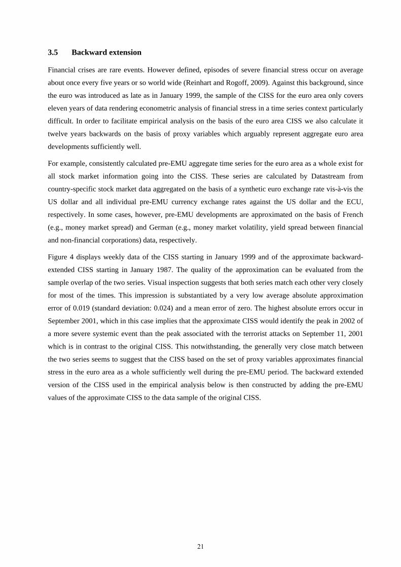
Figure 4 displays weekly data of the CISS starting in January 1999 and of the approximate backward-

extended CISS starting in January 1987. The quality of the approximation can be evaluated from the

sample overlap of the two series. Visual inspection suggests that both series match each other very closely

for most of the times. This impression is substantiated by a very low average absolute approximation

error of 0.019 (standard deviation: 0.024) and a mean error of zero. The highest absolute errors occur in

September 2001, which in this case implies that the approximate CISS would identify the peak in 2002 of

a more severe systemic event than the peak associated with the terrorist attacks on September 11, 2001

which is in contrast to the original CISS. This notwithstanding, the generally very close match between

the two series seems to suggest that the CISS based on the set of proxy variables approximates financial

stress in the euro area as a whole sufficiently well during the pre-EMU period. The backward extended

version of the CISS used in the empirical analysis below is then constructed by adding the pre-EMU

values of the approximate CISS to the data sample of the original CISS.

21

Figure 4. Original and backward-extended proxy-CISS

1987 1989 1991 1993 1995 1997 1999 2001 2003 2005 2007 20090.00

0.25

0.50

0.75

1.00proxy CISS

CISS

Notes: Weekly euro area data from 2 Jan. 1987 to 24 June 2011.

4. Evaluation

We argue that one of the main strengths of the CISS as a financial stress indicator is its explicit

foundation on the notion of systemic risk which the CISS aims to measure by compiling appropriately

transformed individual stress indicators into a single index through application of portfolio-theoretic

economic principles rather than based on purely statistical grounds. We maintain this claim despite the

fact that the CISS is far from being an “ideal” composite indicator in the sense that neither the selection of

raw stress indicators, their transformation, nor their weighting are determined on the basis of an

underlying structural model embedding the concept of systemic risk. The postulated conceptual

superiority of the CISS notwithstanding, this section attempts to evaluate empirically whether the CISS

measures what it is supposed to measure sufficiently accurately, namely the degree of stress prevailing in

the overall financial system.

Evaluating the performance of financial stress indicators is, however, inherently complicated. For

instance, given the fuzziness of the concept of systemic risk, the complexity of modern-world financial

systems and the difficulties in measuring financial stresses and strains, the construction of composite

financial stress indicators involves many arbitrary and subjective choices. As a result, any composite

financial stress indicator has to limit attention to only a few elements of the financial system and to select

from a broad array of largely imperfect measures of stress in the respective market segments. In addition,

reflecting the fact that financial crises are “rare events”, the data samples available for financial stress

indicators are typically rather short, covering only a few historical episodes of financial stress or even

crises and thereby limiting the statistical reliability of empirical analyses. This discrepancy between the

degrees of freedom available in constructing and in testing financial stress indicators, respectively, makes

it extremely difficult to assess whether a particular financial stress index performs well both in absolute

terms (What is a good indicator?) and in relative terms (Which indicator is better?). Against the

22

background of these caveats, the remainder of this section evaluates the performance of the CISS on the

basis of plausibility checks as well as a few statistical and econometric exercises.

4.1 Robustness

The signals issued by a financial stress indicator should be stable over time. This robustness property is

essential for regular usage of the CISS in the practical real-time monitoring of systemic stress, as it avoids

the so-called event reclassification problem. For instance, assume that in a particular point in time a

financial stress indicator suggests that the prevailing level of stress is unusually high by historical

standards. It is then desirable that the indicator still classifies this period as a particularly stressful episode

say ten years hence, i.e. when ten years of data are added to the sample for computing the indicator.

Otherwise no robust historical comparison could be made, and the calculation of certain threshold levels

for the indicator would not make sense either.

In order to limit the event reclassification problem from the outset, we have opted for a procedure that

transforms the raw indicators based on order statistics derived from their cumulative distribution

functions. While Figure A.1 in Appendix 1 illustrates the relative stability of the transformation for all

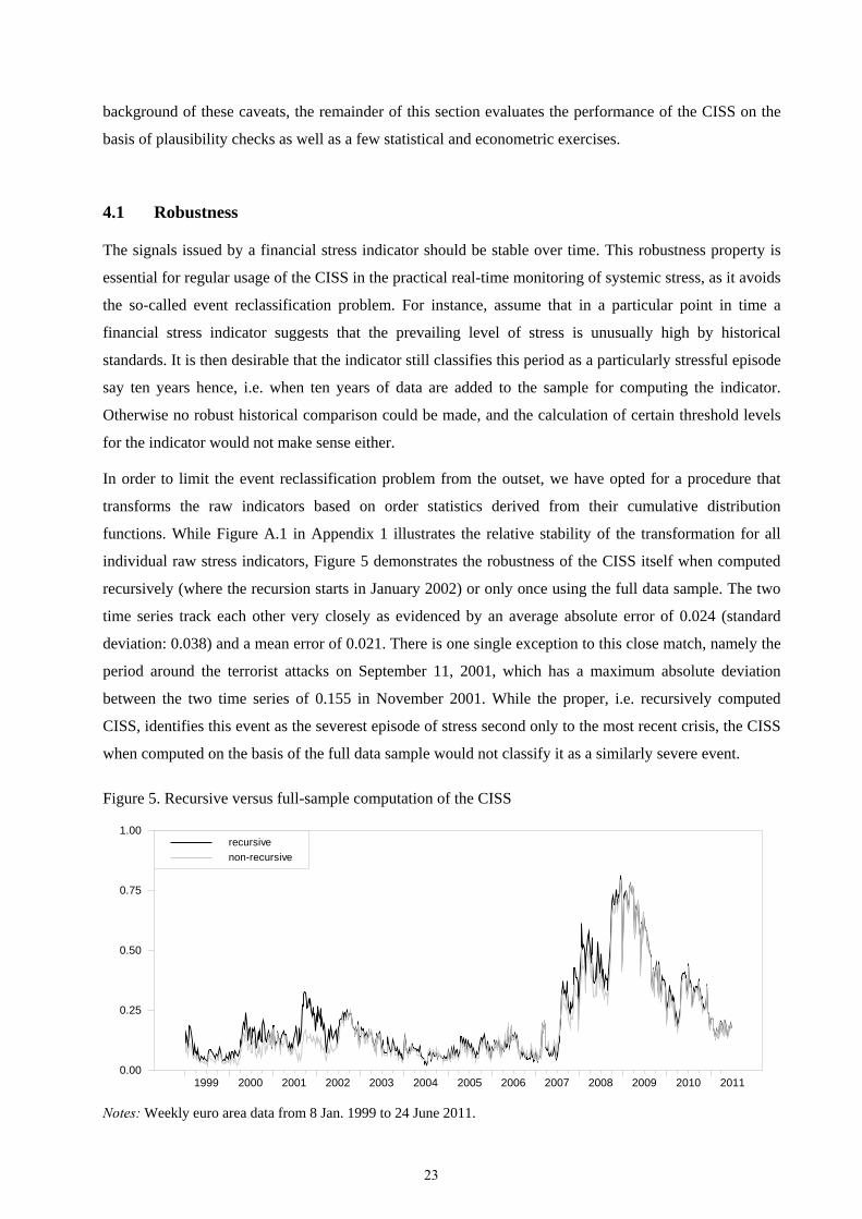
individual raw stress indicators, Figure 5 demonstrates the robustness of the CISS itself when computed

recursively (where the recursion starts in January 2002) or only once using the full data sample. The two

time series track each other very closely as evidenced by an average absolute error of 0.024 (standard

deviation: 0.038) and a mean error of 0.021. There is one single exception to this close match, namely the

period around the terrorist attacks on September 11, 2001, which has a maximum absolute deviation

between the two time series of 0.155 in November 2001. While the proper, i.e. recursively computed

CISS, identifies this event as the severest episode of stress second only to the most recent crisis, the CISS

when computed on the basis of the full data sample would not classify it as a similarly severe event.

Figure 5. Recursive versus full-sample computation of the CISS

1999 2000 2001 2002 2003 2004 2005 2006 2007 2008 2009 2010 20110.00

0.25

0.50

0.75

1.00recursive

non-recursive

Notes: Weekly euro area data from 8 Jan. 1999 to 24 June 2011.

23

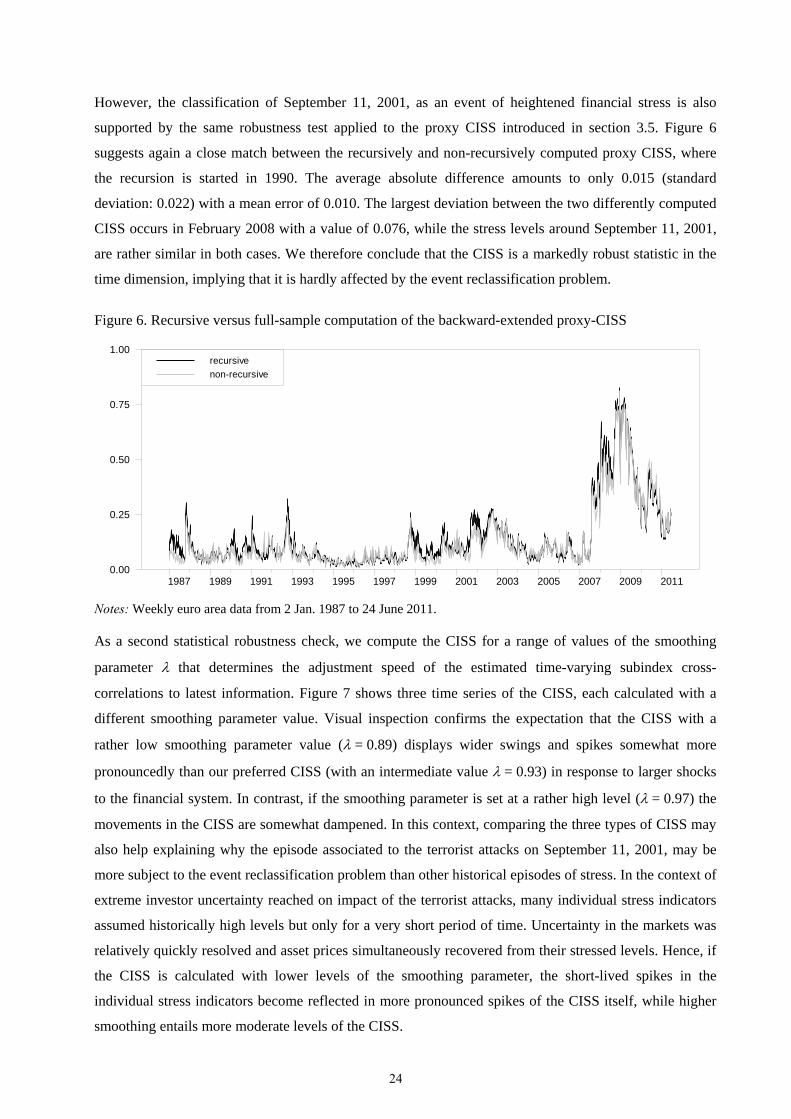
However, the classification of September 11, 2001, as an event of heightened financial stress is also

supported by the same robustness test applied to the proxy CISS introduced in section 3.5. Figure 6

suggests again a close match between the recursively and non-recursively computed proxy CISS, where

the recursion is started in 1990. The average absolute difference amounts to only 0.015 (standard

deviation: 0.022) with a mean error of 0.010. The largest deviation between the two differently computed

CISS occurs in February 2008 with a value of 0.076, while the stress levels around September 11, 2001,

are rather similar in both cases. We therefore conclude that the CISS is a markedly robust statistic in the

time dimension, implying that it is hardly affected by the event reclassification problem.

Figure 6. Recursive versus full-sample computation of the backward-extended proxy-CISS

1987 1989 1991 1993 1995 1997 1999 2001 2003 2005 2007 2009 20110.00

0.25

0.50

0.75

1.00recursive

non-recursive

Notes: Weekly euro area data from 2 Jan. 1987 to 24 June 2011.

As a second statistical robustness check, we compute the CISS for a range of values of the smoothing

parameter that determines the adjustment speed of the estimated time-varying subindex cross-

correlations to latest information. Figure 7 shows three time series of the CISS, each calculated with a

different smoothing parameter value. Visual inspection confirms the expectation that the CISS with a

rather low smoothing parameter value ( = 0.89) displays wider swings and spikes somewhat more

pronouncedly than our preferred CISS (with an intermediate value = 0.93) in response to larger shocks

to the financial system. In contrast, if the smoothing parameter is set at a rather high level ( = 0.97) the

movements in the CISS are somewhat dampened. In this context, comparing the three types of CISS may

also help explaining why the episode associated to the terrorist attacks on September 11, 2001, may be

more subject to the event reclassification problem than other historical episodes of stress. In the context of

extreme investor uncertainty reached on impact of the terrorist attacks, many individual stress indicators

assumed historically high levels but only for a very short period of time. Uncertainty in the markets was

relatively quickly resolved and asset prices simultaneously recovered from their stressed levels. Hence, if

the CISS is calculated with lower levels of the smoothing parameter, the short-lived spikes in the

individual stress indicators become reflected in more pronounced spikes of the CISS itself, while higher

smoothing entails more moderate levels of the CISS.

24

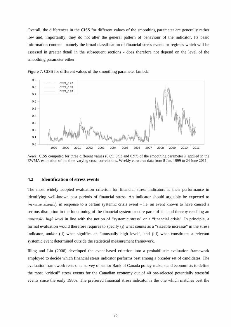
Overall, the differences in the CISS for different values of the smoothing parameter are generally rather

low and, importantly, they do not alter the general pattern of behaviour of the indicator. Its basic

information content - namely the broad classification of financial stress events or regimes which will be

assessed in greater detail in the subsequent sections - does therefore not depend on the level of the

smoothing parameter either.

Figure 7. CISS for different values of the smoothing parameter lambda

1999 2000 2001 2002 2003 2004 2005 2006 2007 2008 2009 2010 20110.0

0.1

0.2

0.3

0.4

0.5

0.6

0.7

0.8

0.9CISS_0.97

CISS_0.89

CISS_0.93

Notes: CISS computed for three different values (0.89, 0.93 and 0.97) of the smoothing parameter applied in the EWMA-estimation of the time-varying cross-correlations. Weekly euro area data from 8 Jan. 1999 to 24 June 2011.

4.2 Identification of stress events

The most widely adopted evaluation criterion for financial stress indicators is their performance in

identifying well-known past periods of financial stress. An indicator should arguably be expected to

increase sizeably in response to a certain systemic crisis event – i.e. an event known to have caused a

serious disruption in the functioning of the financial system or core parts of it – and thereby reaching an

unusually high level in line with the notion of “systemic stress” or a “financial crisis”. In principle, a

formal evaluation would therefore requires to specify (i) what counts as a “sizeable increase” in the stress

indicator, and/or (ii) what signifies an “unusually high level”, and (iii) what constitutes a relevant

systemic event determined outside the statistical measurement framework.

Illing and Liu (2006) developed the event-based criterion into a probabilistic evaluation framework

employed to decide which financial stress indicator performs best among a broader set of candidates. The

evaluation framework rests on a survey of senior Bank of Canada policy-makers and economists to define

the most “critical” stress events for the Canadian economy out of 40 pre-selected potentially stressful

events since the early 1980s. The preferred financial stress indicator is the one which matches best the

25

survey results balancing Type I errors (failure to report a high-stress event) against Type II errors (falsely

reporting a high-stress event).16

While the event-based criterion appears rather obvious and straight-forward, it still suffers from

substantial conceptual and measurement problems. First, in a certain sense it relies on knowing a priori

what the indicator is supposed to measure and detect in the first place, namely systemic stress and

financial crises, respectively. While it is relatively easy to identify historical events which are generally

perceived as having caused serious disruptions in certain segments of the financial system, it is far less

clear to establish which ones were also posing a truly systemic threat to the economy. Moreover, and in

particular when the data are measured at a higher frequency, the criterion also requires that one knows (or

assumes) when the stress began and when it ended.17 Second, the focus on popular crisis events excludes

periods of systemic stress which are not associated with a specific triggering event but which rather build

up gradually over time as a result of cumulated smaller pieces of bad news. The “dot-com” boom and bust

episode around the turn of the millennium may exemplify such a case. While the prices of high-tech

stocks peaked in the first quarter of 2000 after several years of strong appreciation, the subsequent crash

in the high-tech market segment still came in “instalments”, dragging on for quite a while, and was only

during later stages occasionally associated with specific crisis events. Hence, evaluation approaches

relying on “crises defined by events” are likely to miss such more hidden periods of systemic stress, while

“crises defined by quantitative thresholds” determined on the basis of financial stress indicators are less

prone to such Type I errors.18 In the light of these problems, we argue against relying too strongly on a

formalised version of the event-criterion when assessing and comparing the performance of financial

stress indicators.19

We prefer assessing whether peaks in the CISS are generally associated with well-known historical stress

events similar to the approach taken by, e.g., Hakkio and Keeton (2009). Figure 8 illustrates that the

sharpest spikes in the CISS indeed tend to occur around very well-known events which caused, at least

temporarily, severe stress in the global financial system. The first major stress event in the sample is the

stock market crash in October 1987. On October 19, the US stock market experienced its largest one-day

loss in market valuations ever, causing extreme stress in the financial industry. However, stress subsided

relatively quickly when market participants realised that financial firms had been able to remain

financially sound (Cardarelli, Elekdag and Lall 2011). The CISS spiked up again in early 1990 when

16 In the evaluation of the indicators’ ability to predict stress events, the authors assume that a financial stress indicator signals a high-stress event if it passes an arbitrary threshold of two standard deviations above its historical mean. 17 In fact, continuous-scale financial stress indicators such as the CISS can exactly be used as tools to delineate the start and end points of financial crises. 18 The distinction between “crises defined by events” and “crises defined by quantitative thresholds” is borrowed from Reinhart and Rogoff (2009). Sometimes this distinction is blurred, namely when events are identified on the basis of quantitative thresholds for certain key indicators. 19 The problems with the event-criterion are further aggravated in the case of a financial stress indicator for the euro area as a whole. For example, a formalisation of the criterion would require an assumption as to which specific events posed a threat to the financial systems of a sufficiently large part of the currency area.

26

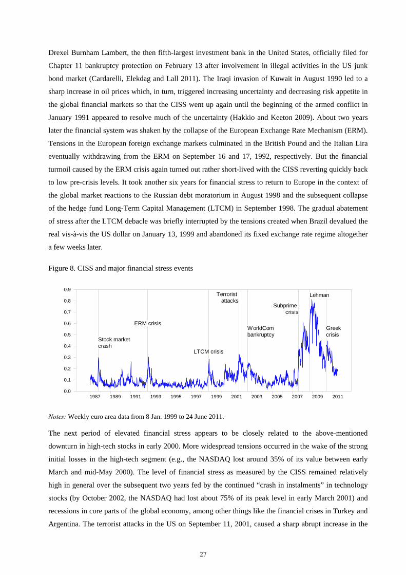
Drexel Burnham Lambert, the then fifth-largest investment bank in the United States, officially filed for

Chapter 11 bankruptcy protection on February 13 after involvement in illegal activities in the US junk

bond market (Cardarelli, Elekdag and Lall 2011). The Iraqi invasion of Kuwait in August 1990 led to a

sharp increase in oil prices which, in turn, triggered increasing uncertainty and decreasing risk appetite in

the global financial markets so that the CISS went up again until the beginning of the armed conflict in

January 1991 appeared to resolve much of the uncertainty (Hakkio and Keeton 2009). About two years

later the financial system was shaken by the collapse of the European Exchange Rate Mechanism (ERM).

Tensions in the European foreign exchange markets culminated in the British Pound and the Italian Lira

eventually withdrawing from the ERM on September 16 and 17, 1992, respectively. But the financial

turmoil caused by the ERM crisis again turned out rather short-lived with the CISS reverting quickly back

to low pre-crisis levels. It took another six years for financial stress to return to Europe in the context of

the global market reactions to the Russian debt moratorium in August 1998 and the subsequent collapse

of the hedge fund Long-Term Capital Management (LTCM) in September 1998. The gradual abatement

of stress after the LTCM debacle was briefly interrupted by the tensions created when Brazil devalued the

real vis-à-vis the US dollar on January 13, 1999 and abandoned its fixed exchange rate regime altogether

a few weeks later.

Figure 8. CISS and major financial stress events

1987 1989 1991 1993 1995 1997 1999 2001 2003 2005 2007 2009 20110.0

0.1

0.2

0.3

0.4

0.5

0.6

0.7

0.8

0.9

Stock market crash

ERM crisis

LTCM crisis

Terrorist attacks

WorldCom bankruptcy

Subprime crisis

Lehman

Greek crisis

Notes: Weekly euro area data from 8 Jan. 1999 to 24 June 2011.

The next period of elevated financial stress appears to be closely related to the above-mentioned

downturn in high-tech stocks in early 2000. More widespread tensions occurred in the wake of the strong

initial losses in the high-tech segment (e.g., the NASDAQ lost around 35% of its value between early

March and mid-May 2000). The level of financial stress as measured by the CISS remained relatively

high in general over the subsequent two years fed by the continued “crash in instalments” in technology

stocks (by October 2002, the NASDAQ had lost about 75% of its peak level in early March 2001) and

recessions in core parts of the global economy, among other things like the financial crises in Turkey and

Argentina. The terrorist attacks in the US on September 11, 2001, caused a sharp abrupt increase in the

27

CISS in between. Investors soon realised, though, that their initial fears about the potential financial and

real economic impacts of the attacks were exaggerated such that the global financial system recovered

relatively quickly from this severe shock. The accounting scandals around Enron and WorldCom (filing

for bankruptcy in December 2001 and July 2002, by the time the largest defaults in US corporate history)

further intensified financial strains by increasing the uncertainty about the health of the corporate sector

and the economy in general.

However, none of the above-mentioned events was able to push the CISS towards levels reached during

the most recent financial and economic crisis. The CISS first signalled an extreme level of stress in

August 2007, when BNP Paribas suspended three investment funds that invested in asset backed

securities linked to subprime mortgage debt which had become totally illiquid. Many announcements of

credit-losses and write-downs by banks, mortgage lenders and other institutional investors followed,

driving the CISS up further until it reached another peak when Bear Stearns collapsed in March 2008.

The situation remained jittery due to continued bad news such as the failure of IndyMac and emerging

signs of substantial trouble in Freddie Mae and Freddie Mac. The CISS surged again and achieved its

third largest value in September 2008, when Lehman Brothers filed for bankruptcy protection and AIG

was rescued to avoid bankruptcy. The index reached its historical maximum in November 2008 when the

US plan to buy toxic assets under the Troubled Asset Relief Program (TARP) was abandoned, which

undermined global market confidence. After November 2008 the CISS signalled a steady decline in

financial stress until mid-April 2010 when serious concerns about sovereign credit risk in the euro area

emerged.

To sum up, it appears that all extreme peaks in the CISS can be associated with specific financial stress

events suggesting that it does not suffer from type II errors. It is harder to judge whether it also performs

well on the dimension of type I errors, i.e. whether there are severe crises which it failed to indicate.

Potential candidates in this regard are the global bond market crisis and the Mexican peso crisis both in

1994 and the Asian crisis in 1997, for instance. The CISS suggests that these events did not trigger

significant systemic stress in the euro area financial system as a whole but rather represented more

isolated tensions in specific market segments and other parts of the world economy.20 Developments of

the CISS appear in general rather plausible, not least because it singles out very clearly the recent

financial and economic crisis as the most stressful period over the past quarter of a century of available

data for the euro area, comparable probably only to the Great Depression.

20 This is broadly consistent with findings from the international contagion literature (e.g., Bekaert, Harvey and Ang 2005) Furthermore, the Kansas City Financial Stress Index presented in Hakkio and Keeton (2006) does not identify these events as particularly stressful for the US financial system either.

28

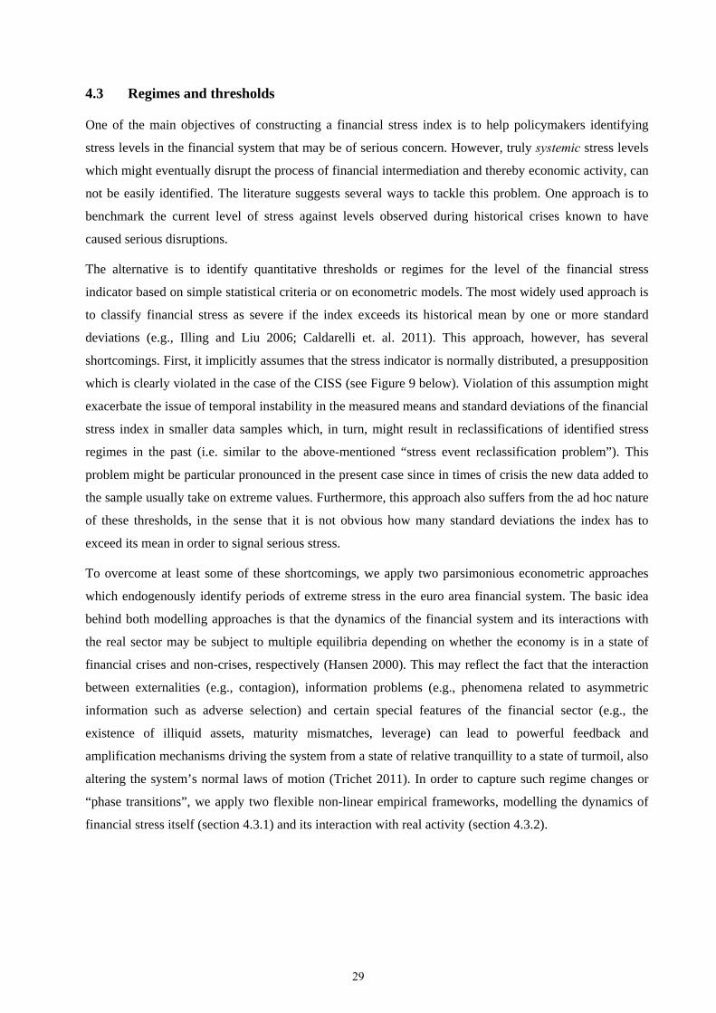
4.3 Regimes and thresholds

One of the main objectives of constructing a financial stress index is to help policymakers identifying

stress levels in the financial system that may be of serious concern. However, truly systemic stress levels

which might eventually disrupt the process of financial intermediation and thereby economic activity, can

not be easily identified. The literature suggests several ways to tackle this problem. One approach is to

benchmark the current level of stress against levels observed during historical crises known to have

caused serious disruptions.

The alternative is to identify quantitative thresholds or regimes for the level of the financial stress

indicator based on simple statistical criteria or on econometric models. The most widely used approach is

to classify financial stress as severe if the index exceeds its historical mean by one or more standard

deviations (e.g., Illing and Liu 2006; Caldarelli et. al. 2011). This approach, however, has several

shortcomings. First, it implicitly assumes that the stress indicator is normally distributed, a presupposition

which is clearly violated in the case of the CISS (see Figure 9 below). Violation of this assumption might

exacerbate the issue of temporal instability in the measured means and standard deviations of the financial

stress index in smaller data samples which, in turn, might result in reclassifications of identified stress

regimes in the past (i.e. similar to the above-mentioned “stress event reclassification problem”). This

problem might be particular pronounced in the present case since in times of crisis the new data added to

the sample usually take on extreme values. Furthermore, this approach also suffers from the ad hoc nature

of these thresholds, in the sense that it is not obvious how many standard deviations the index has to

exceed its mean in order to signal serious stress.

To overcome at least some of these shortcomings, we apply two parsimonious econometric approaches

which endogenously identify periods of extreme stress in the euro area financial system. The basic idea

behind both modelling approaches is that the dynamics of the financial system and its interactions with

the real sector may be subject to multiple equilibria depending on whether the economy is in a state of

financial crises and non-crises, respectively (Hansen 2000). This may reflect the fact that the interaction

between externalities (e.g., contagion), information problems (e.g., phenomena related to asymmetric

information such as adverse selection) and certain special features of the financial sector (e.g., the

existence of illiquid assets, maturity mismatches, leverage) can lead to powerful feedback and

amplification mechanisms driving the system from a state of relative tranquillity to a state of turmoil, also

altering the system’s normal laws of motion (Trichet 2011). In order to capture such regime changes or

“phase transitions”, we apply two flexible non-linear empirical frameworks, modelling the dynamics of

financial stress itself (section 4.3.1) and its interaction with real activity (section 4.3.2).

29

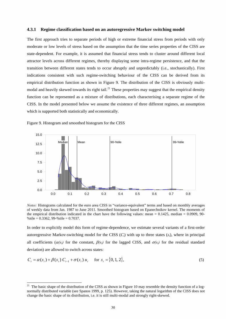
4.3.1 Regime classification based on an autoregressive Markov switching model

The first approach tries to separate periods of high or extreme financial stress from periods with only

moderate or low levels of stress based on the assumption that the time series properties of the CISS are

state-dependent. For example, it is assumed that financial stress tends to cluster around different local

attractor levels across different regimes, thereby displaying some intra-regime persistence, and that the

transition between different states tends to occur abruptly and unpredictably (i.e., stochastically). First

indications consistent with such regime-switching behaviour of the CISS can be derived from its

empirical distribution function as shown in Figure 9. The distribution of the CISS is obviously multi-

modal and heavily skewed towards its right tail.21 These properties may suggest that the empirical density

function can be represented as a mixture of distributions, each characterising a separate regime of the

CISS. In the model presented below we assume the existence of three different regimes, an assumption

which is supported both statistically and economically.

Figure 9. Histogram and smoothed histogram for the CISS

0.0 0.1 0.2 0.3 0.4 0.5 0.6 0.7 0.80.0

2.5

5.0

7.5

10.0

12.5

15.0

MeanMedian 90-%tile 99-%tile

Notes: Histograms calculated for the euro area CISS in “variance-equivalent” terms and based on monthly averages of weekly data from Jan. 1987 to June 2011. Smoothed histogram based on Epanechnikov kernel. The moments of the empirical distribution indicated in the chart have the following values: mean = 0.1425, median = 0.0909, 90-%tile = 0.3362, 99-%tile = 0.7037.

In order to explicitly model this form of regime-dependence, we estimate several variants of a first-order

autoregressive Markov-switching model for the CISS (Ct) with up to three states (st), where in principal

all coefficients ((st) for the constant, (st) for the lagged CISS, and (st) for the residual standard

deviation) are allowed to switch across states:

tttttt usCssC )()()( 1 for 2,1,0ts , (5)

21 The basic shape of the distribution of the CISS as shown in Figure 10 may resemble the density function of a log-normally distributed variable (see Spanos 1999, p. 125). However, taking the natural logarithm of the CISS does not change the basic shape of its distribution, i.e. it is still multi-modal and strongly right-skewed.

30

with residuals ut assumed to be standard, normal, independent and identically distributed (NID). The

model is completed with the assumption that the stochastic process generating the states st follows an

ergodic first-order Markov chain with transition probabilities jitt pjsisp |1 collected in the

transition matrix P:

2|12|01|11|00|10|0

2|11|10|1

2|01|00|0

2|21|20|2

2|11|10|1

2|01|00|0

111 pppppp

ppp

ppp

ppp

ppp

ppp

P , (6)

where the conditional probabilities in the third row of the right-hand matrix have been replaced by the

usual adding-up constraints for probabilities (implying that for a model with three regimes only six out of

nine transition probabilities can be estimated independently). The assumption that states follow a first-

order Markov process implies that next period’s regime only depends on the current regime but not on

previous ones (see, e.g., Hamilton 1994).

Table 2. Comparing different specifications of Markov-switching autoregressive models for the CISS

Scaled residuals (p-values)

ModelLog-

likelihoodNo. of

parameters AIC RCM Normality ARCH(1)Auto-

correlation

MS(3)-DR(1) 626.868 11 -4.2038 19.38 0.983 0.304 0.160MS(3)-AR(1) 633.452 14 -4.2283 25.95 0.868 0.149 0.202MS(2)-AR(1) 607.684 8 -4.0934 23.26 0.026 0.851 0.416

Notes: The RCM is the regime classification measure in its refined version of Baele (2005) as defined in equation (7) in the main text. RCM lies between zero and 100 where lower values are associated with better regime classification. The model abbreviations are to be read as follows: MS(s) stands for a Markov-switching model with s states. AR(p) denotes an autoregression model of order p in which both the intercept and the slope coefficient can switch across regimes. DR(p) restricts the slope coefficient to be identical across regimes. Estimations based on monthly averages of weekly data for the euro area from Jan. 1987 to June 2011.

Our preferred model specification is an autoregressive process of order one (AR(1)) with three regimes in

which the intercept and the residual variance are allowed to switch while the slope coefficient is restricted

to be identical across all three regimes.22 Following Doornik (2011) we call this a Markov-switching

dynamic regression model labelled MS(3)-DR(1) in contrast to a fully-fledged MS(3)-AR(1) model in

which also the slope coefficients can vary across regimes. In general, both model specifications deliver

quite similar quantitative results (e.g., statistical model properties, regime classification etc.). Some

summary statistics for both models are listed in Table 2 above. For instance, the MS(3)-AR(1) model

appears superior in terms of log-likelihood values and information criteria (AIC). The better fit compared

to the MS(3)-DR(1) is derived from the fact that it tracks the CISS somewhat better during the height of

the recent crisis after the collapse of Lehman Brothers (see the first panel of Figure 10 for the fit of the

MS(3)-DR(1) model). In terms of the scaled residuals, both model specifications survive standard

22 The lag order one is strongly supported by standard information criteria as well as by testing corresponding exclusion restrictions in the models discussed below with higher lag orders.

31

misspecification tests as shown in the last three columns of Table 2, where the p-values are higher in two

out of three cases for the MS(3)-DR(1) model. The fact that the null hypothesis of scaled residuals being

NID can not be rejected statistically supports our basic assumption that the right-skewed multi-modal

distribution of the CISS can be approximately modelled as a mixture of three normal distributions (the

raw and the scaled residuals are plotted in the second panel of Figure 10).23 The main argument speaking

in favour of the MS(3)-DR(1) model - apart from its more parsimonious representation (only 11 estimated

parameters instead of 14) - is its sharper regime classification as reflected in the Regime Classification

Measure (RCM) proposed by Ang and Bekaert (2002) and refined by Baele (2005) for multiple regimes

(see the fifth column of Table 2).24 The RCM is calculated as

T

t

K

jtj K

pTK

KKRCM

1 1

2

,

11

11100)( , (7)

where K is the number of regimes, T is the number of observations, and pj,t is the smoothed probability to

be in regime j = 1, . . . , K at time t. The RCM is normalised to lie between a value of zero and a value of

one hundred. A value of zero indicates perfect regime classification, as in this case one of the (smoothed)

regime probabilities would be unity at all the times. On the other hand, a value of one hundred implies

that the model reveals no information about the prevailing regimes since all regimes have the same

probability all the time. Weak regime inference, indicated by values close to one hundred, implies that a

Markov-switching model cannot successfully distinguish between regimes from the behaviour of the data

and may thus indicate misspecification (Sarno, Valente and Wohar, 2003). The RCM for the MS(3)-

DR(1) is indeed very low with a value of 19.38. The sharp regime identification of this model can also be

illustrated by the fact that the dominant regime has an average sample probability of 0.91 (see also the last

three panels of Figure 10) and is never below 0.5. The RCM value of 25.95 for the MS(3)-AR(1) is also

sufficiently small to indicate a successful regime classification, with an average probability of the

dominant regime of 0.88. This notwithstanding, the time series of the probability of the highest stress

regime the MS(3)-DR(1) model may also appear slightly more plausible compared with that of the

MS(3)-AR(1) model. For instance, the dynamic regression model singles out more clearly the recent

crisis as the most stressful period, only accompanied by the months of September and October 2001 as a

short period of similar levels of stress. The autoregressive model with state-dependent slope coefficients,

in contrast, associates four more short-lived spikes in the CISS with a crisis state, and it also advances the

start of the subprime crisis to March 2007 instead of August 2007.

23 The approximation seems to work rather well although the autoregressive Markov-switching model does not constrain the CISS to stay within its lower (zero) and upper (one) bounds. This claim is supported by a Monte-Carlo simulation generating 10,000 artificial time series of the CISS based on the MS(3)-DR(1) model. The simulation delivers 2,940,000 observations of which only 91 (0.0030952%) assume a negative value, while values greater than one even never occur. Further details of the simulation are available upon request. 24 For applications of the RCM see, e.g., Domanski and Kremer (2000) and Sarno, Valente and Wohar (2003).

32

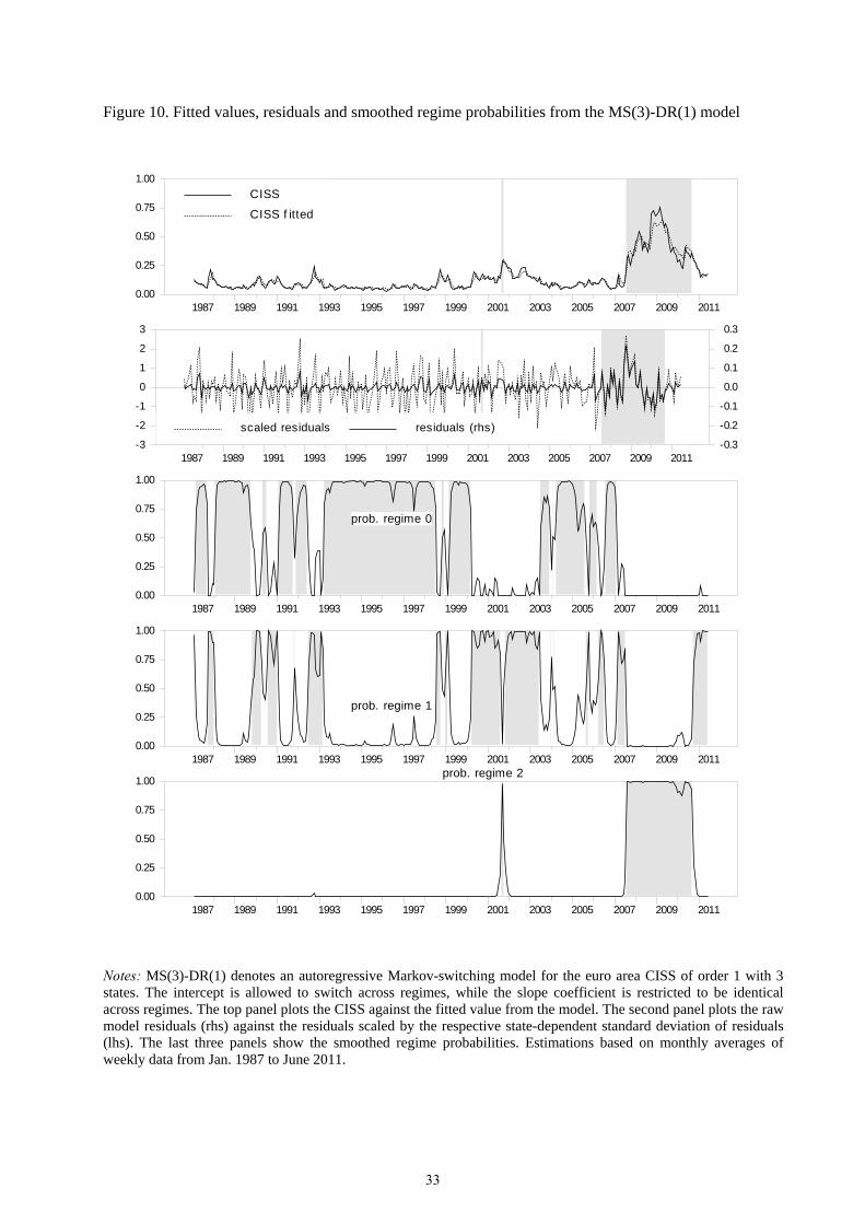
Figure 10. Fitted values, residuals and smoothed regime probabilities from the MS(3)-DR(1) model

1987 1989 1991 1993 1995 1997 1999 2001 2003 2005 2007 2009 20110.00

0.25

0.50

0.75

1.00

CISS

CISS f itted

1987 1989 1991 1993 1995 1997 1999 2001 2003 2005 2007 2009 2011-3

-2

-1

0

1

2

3

-0.3

-0.2

-0.1

0.0

0.1

0.2

0.3

scaled residuals residuals (rhs)

1987 1989 1991 1993 1995 1997 1999 2001 2003 2005 2007 2009 20110.00

0.25

0.50

0.75

1.00

prob. regime 0

1987 1989 1991 1993 1995 1997 1999 2001 2003 2005 2007 2009 20110.00

0.25

0.50

0.75

1.00

prob. regime 1

1987 1989 1991 1993 1995 1997 1999 2001 2003 2005 2007 2009 20110.00

0.25

0.50

0.75

1.00prob. regime 2

Notes: MS(3)-DR(1) denotes an autoregressive Markov-switching model for the euro area CISS of order 1 with 3 states. The intercept is allowed to switch across regimes, while the slope coefficient is restricted to be identical across regimes. The top panel plots the CISS against the fitted value from the model. The second panel plots the raw model residuals (rhs) against the residuals scaled by the respective state-dependent standard deviation of residuals (lhs). The last three panels show the smoothed regime probabilities. Estimations based on monthly averages of weekly data from Jan. 1987 to June 2011.

33

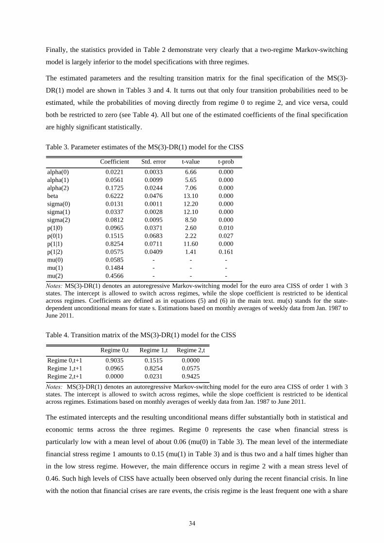
Finally, the statistics provided in Table 2 demonstrate very clearly that a two-regime Markov-switching

model is largely inferior to the model specifications with three regimes.

The estimated parameters and the resulting transition matrix for the final specification of the MS(3)-

DR(1) model are shown in Tables 3 and 4. It turns out that only four transition probabilities need to be

estimated, while the probabilities of moving directly from regime 0 to regime 2, and vice versa, could

both be restricted to zero (see Table 4). All but one of the estimated coefficients of the final specification

are highly significant statistically.

Table 3. Parameter estimates of the MS(3)-DR(1) model for the CISS

Coefficient Std. error t-value t-prob

alpha(0) 0.0221 0.0033 6.66 0.000alpha(1) 0.0561 0.0099 5.65 0.000alpha(2) 0.1725 0.0244 7.06 0.000beta 0.6222 0.0476 13.10 0.000sigma(0) 0.0131 0.0011 12.20 0.000sigma(1) 0.0337 0.0028 12.10 0.000sigma(2) 0.0812 0.0095 8.50 0.000p(1|0) 0.0965 0.0371 2.60 0.010p(0|1) 0.1515 0.0683 2.22 0.027p(1|1) 0.8254 0.0711 11.60 0.000p(1|2) 0.0575 0.0409 1.41 0.161mu(0) 0.0585 - - -mu(1) 0.1484 - - -mu(2) 0.4566 - - -

Notes: MS(3)-DR(1) denotes an autoregressive Markov-switching model for the euro area CISS of order 1 with 3 states. The intercept is allowed to switch across regimes, while the slope coefficient is restricted to be identical across regimes. Coefficients are defined as in equations (5) and (6) in the main text. mu(s) stands for the state-dependent unconditional means for state s. Estimations based on monthly averages of weekly data from Jan. 1987 to June 2011.

Table 4. Transition matrix of the MS(3)-DR(1) model for the CISS

Regime 0,t Regime 1,t Regime 2,t

Regime 0,t+1 0.9035 0.1515 0.0000Regime 1,t+1 0.0965 0.8254 0.0575Regime 2,t+1 0.0000 0.0231 0.9425

Notes: MS(3)-DR(1) denotes an autoregressive Markov-switching model for the euro area CISS of order 1 with 3 states. The intercept is allowed to switch across regimes, while the slope coefficient is restricted to be identical across regimes. Estimations based on monthly averages of weekly data from Jan. 1987 to June 2011.

The estimated intercepts and the resulting unconditional means differ substantially both in statistical and

economic terms across the three regimes. Regime 0 represents the case when financial stress is

particularly low with a mean level of about 0.06 (mu(0) in Table 3). The mean level of the intermediate

financial stress regime 1 amounts to 0.15 (mu(1) in Table 3) and is thus two and a half times higher than

in the low stress regime. However, the main difference occurs in regime 2 with a mean stress level of

0.46. Such high levels of CISS have actually been observed only during the recent financial crisis. In line

with the notion that financial crises are rare events, the crisis regime is the least frequent one with a share

34

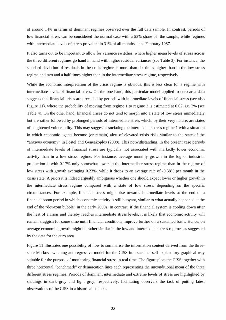
of around 14% in terms of dominant regimes observed over the full data sample. In contrast, periods of

low financial stress can be considered the normal case with a 55% share of the sample, while regimes

with intermediate levels of stress prevalent in 31% of all months since February 1987.

It also turns out to be important to allow for variance switches, where higher mean levels of stress across

the three different regimes go hand in hand with higher residual variances (see Table 3). For instance, the

standard deviation of residuals in the crisis regime is more than six times higher than in the low stress

regime and two and a half times higher than in the intermediate stress regime, respectively.

While the economic interpretation of the crisis regime is obvious, this is less clear for a regime with

intermediate levels of financial stress. On the one hand, this particular model applied to euro area data

suggests that financial crises are preceded by periods with intermediate levels of financial stress (see also

Figure 11), where the probability of moving from regime 1 to regime 2 is estimated at 0.02, i.e. 2% (see

Table 4). On the other hand, financial crises do not tend to morph into a state of low stress immediately

but are rather followed by prolonged periods of intermediate stress which, by their very nature, are states

of heightened vulnerability. This may suggest associating the intermediate stress regime 1 with a situation

in which economic agents become (or remain) alert of elevated crisis risks similar to the state of the

“anxious economy” in Fostel and Geneakoplos (2008). This notwithstanding, in the present case periods

of intermediate levels of financial stress are typically not associated with markedly lower economic

activity than in a low stress regime. For instance, average monthly growth in the log of industrial

production is with 0.17% only somewhat lower in the intermediate stress regime than in the regime of

low stress with growth averaging 0.23%, while it drops to an average rate of -0.38% per month in the

crisis state. A priori it is indeed arguably ambiguous whether one should expect lower or higher growth in

the intermediate stress regime compared with a state of low stress, depending on the specific

circumstances. For example, financial stress might rise towards intermediate levels at the end of a

financial boom period in which economic activity is still buoyant, similar to what actually happened at the

end of the “dot-com bubble” in the early 2000s. In contrast, if the financial system is cooling down after

the heat of a crisis and thereby reaches intermediate stress levels, it is likely that economic activity will

remain sluggish for some time until financial conditions improve further on a sustained basis. Hence, on

average economic growth might be rather similar in the low and intermediate stress regimes as suggested

by the data for the euro area.

Figure 11 illustrates one possibility of how to summarise the information content derived from the three-

state Markov-switching autoregressive model for the CISS in a succinct self-explanatory graphical way

suitable for the purpose of monitoring financial stress in real time. The figure plots the CISS together with

three horizontal “benchmark” or demarcation lines each representing the unconditional mean of the three

different stress regimes. Periods of dominant intermediate and extreme levels of stress are highlighted by

shadings in dark grey and light grey, respectively, facilitating observers the task of putting latest

observations of the CISS in a historical context.

35

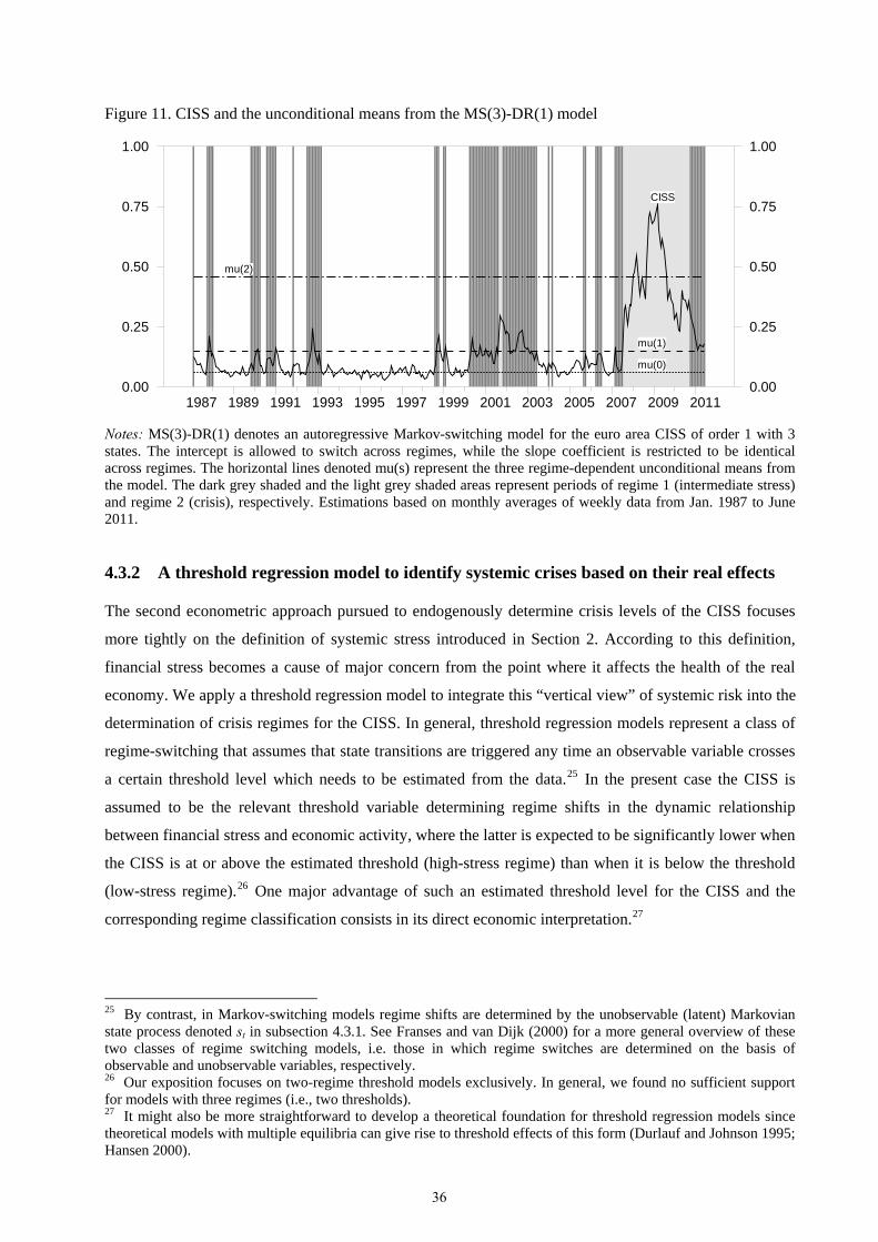
Figure 11. CISS and the unconditional means from the MS(3)-DR(1) model

1987 1989 1991 1993 1995 1997 1999 2001 2003 2005 2007 2009 20110.00

0.25

0.50

0.75

1.00

0.00

0.25

0.50

0.75

1.00

CISS

mu(0)

mu(1)

mu(2)

Notes: MS(3)-DR(1) denotes an autoregressive Markov-switching model for the euro area CISS of order 1 with 3 states. The intercept is allowed to switch across regimes, while the slope coefficient is restricted to be identical across regimes. The horizontal lines denoted mu(s) represent the three regime-dependent unconditional means from the model. The dark grey shaded and the light grey shaded areas represent periods of regime 1 (intermediate stress) and regime 2 (crisis), respectively. Estimations based on monthly averages of weekly data from Jan. 1987 to June 2011.

4.3.2 A threshold regression model to identify systemic crises based on their real effects

The second econometric approach pursued to endogenously determine crisis levels of the CISS focuses

more tightly on the definition of systemic stress introduced in Section 2. According to this definition,

financial stress becomes a cause of major concern from the point where it affects the health of the real

economy. We apply a threshold regression model to integrate this “vertical view” of systemic risk into the

determination of crisis regimes for the CISS. In general, threshold regression models represent a class of

regime-switching that assumes that state transitions are triggered any time an observable variable crosses

a certain threshold level which needs to be estimated from the data.25 In the present case the CISS is

assumed to be the relevant threshold variable determining regime shifts in the dynamic relationship

between financial stress and economic activity, where the latter is expected to be significantly lower when

the CISS is at or above the estimated threshold (high-stress regime) than when it is below the threshold

(low-stress regime).26 One major advantage of such an estimated threshold level for the CISS and the

corresponding regime classification consists in its direct economic interpretation.27

25 By contrast, in Markov-switching models regime shifts are determined by the unobservable (latent) Markovian state process denoted st in subsection 4.3.1. See Franses and van Dijk (2000) for a more general overview of these two classes of regime switching models, i.e. those in which regime switches are determined on the basis of observable and unobservable variables, respectively. 26 Our exposition focuses on two-regime threshold models exclusively. In general, we found no sufficient support for models with three regimes (i.e., two thresholds). 27 It might also be more straightforward to develop a theoretical foundation for threshold regression models since theoretical models with multiple equilibria can give rise to threshold effects of this form (Durlauf and Johnson 1995; Hansen 2000).

36

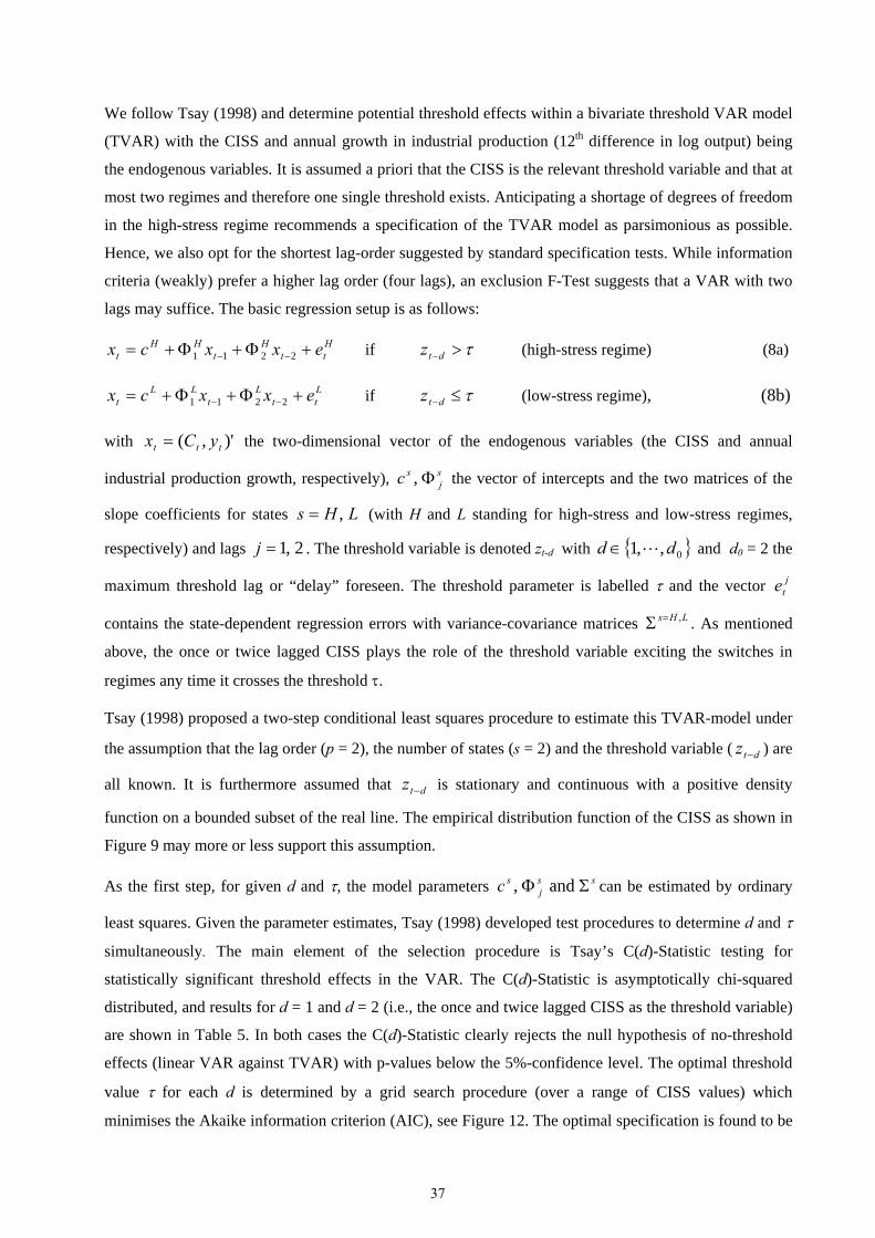
We follow Tsay (1998) and determine potential threshold effects within a bivariate threshold VAR model

(TVAR) with the CISS and annual growth in industrial production (12th difference in log output) being

the endogenous variables. It is assumed a priori that the CISS is the relevant threshold variable and that at

most two regimes and therefore one single threshold exists. Anticipating a shortage of degrees of freedom

in the high-stress regime recommends a specification of the TVAR model as parsimonious as possible.

Hence, we also opt for the shortest lag-order suggested by standard specification tests. While information

criteria (weakly) prefer a higher lag order (four lags), an exclusion F-Test suggests that a VAR with two

lags may suffice. The basic regression setup is as follows:

Htt

Ht

HHt exxcx 2211 if dtz (high-stress regime) (8a)

Ltt

Lt

LLt exxcx 2211 if dtz (low-stress regime), (8b)

with the two-dimensional vector of the endogenous variables (the CISS and annual

industrial production growth, respectively), the vector of intercepts and the two matrices of the

slope coefficients for states (with H and L standing for high-stress and low-stress regimes,

respectively) and lags

)',( ttt yCx

sj

sc ,

LHs ,

2,1j . The threshold variable is denoted zt-d with 0,,1 dd and d0 = 2 the

maximum threshold lag or “delay” foreseen. The threshold parameter is labelled and the vector

contains the state-dependent regression errors with variance-covariance matrices . As mentioned

above, the once or twice lagged CISS plays the role of the threshold variable exciting the switches in

regimes any time it crosses the threshold .

jte

LHs ,

Tsay (1998) proposed a two-step conditional least squares procedure to estimate this TVAR-model under

the assumption that the lag order (p = 2), the number of states (s = 2) and the threshold variable ( ) are

all known. It is furthermore assumed that is stationary and continuous with a positive density

function on a bounded subset of the real line. The empirical distribution function of the CISS as shown in

Figure 9 may more or less support this assumption.

dtz

dtz

As the first step, for given d and , the model parameters can be estimated by ordinary

least squares. Given the parameter estimates, Tsay (1998) developed test procedures to determine d and

simultaneously. The main element of the selection procedure is Tsay’s C(d)-Statistic testing for

statistically significant threshold effects in the VAR. The C(d)-Statistic is asymptotically chi-squared

distributed, and results for d = 1 and d = 2 (i.e., the once and twice lagged CISS as the threshold variable)

are shown in Table 5. In both cases the C(d)-Statistic clearly rejects the null hypothesis of no-threshold

effects (linear VAR against TVAR) with p-values below the 5%-confidence level. The optimal threshold

value for each d is determined by a grid search procedure (over a range of CISS values) which

minimises the Akaike information criterion (AIC), see Figure 12. The optimal specification is found to be

ssj

sc and,

37

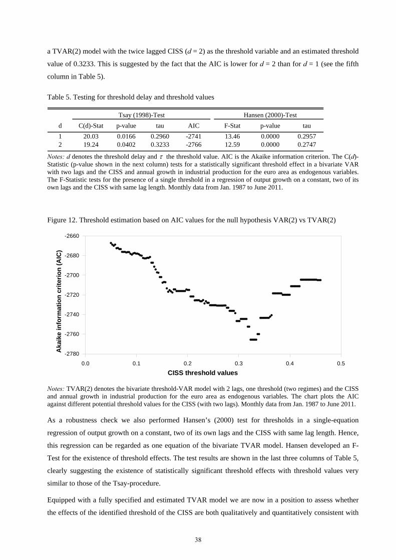
a TVAR(2) model with the twice lagged CISS (d = 2) as the threshold variable and an estimated threshold

value of 0.3233. This is suggested by the fact that the AIC is lower for d = 2 than for d = 1 (see the fifth

column in Table 5).

Table 5. Testing for threshold delay and threshold values

Hansen (2000)-Test

d C(d)-Stat p-value tau AIC F-Stat p-value tau

1 20.03 0.0166 0.2960 -2741 13.46 0.0000 0.29572 19.24 0.0402 0.3233 -2766 12.59 0.0000 0.2747

Tsay (1998)-Test

Notes: d denotes the threshold delay and the threshold value. AIC is the Akaike information criterion. The C(d)-Statistic (p-value shown in the next column) tests for a statistically significant threshold effect in a bivariate VAR with two lags and the CISS and annual growth in industrial production for the euro area as endogenous variables. The F-Statistic tests for the presence of a single threshold in a regression of output growth on a constant, two of its own lags and the CISS with same lag length. Monthly data from Jan. 1987 to June 2011.

Figure 12. Threshold estimation based on AIC values for the null hypothesis VAR(2) vs TVAR(2)

CISS threshold values

Aka

ike

info

rmat

ion

cri

teri

on

(A

IC)

0.0 0.1 0.2 0.3 0.4 0.5

-2780

-2760

-2740

-2720

-2700

-2680

-2660

Notes: TVAR(2) denotes the bivariate threshold-VAR model with 2 lags, one threshold (two regimes) and the CISS and annual growth in industrial production for the euro area as endogenous variables. The chart plots the AIC against different potential threshold values for the CISS (with two lags). Monthly data from Jan. 1987 to June 2011.

As a robustness check we also performed Hansen’s (2000) test for thresholds in a single-equation

regression of output growth on a constant, two of its own lags and the CISS with same lag length. Hence,

this regression can be regarded as one equation of the bivariate TVAR model. Hansen developed an F-

Test for the existence of threshold effects. The test results are shown in the last three columns of Table 5,

clearly suggesting the existence of statistically significant threshold effects with threshold values very

similar to those of the Tsay-procedure.

Equipped with a fully specified and estimated TVAR model we are now in a position to assess whether

the effects of the identified threshold of the CISS are both qualitatively and quantitatively consistent with

38

our expectation that extreme systemic financial stress exerts strong negative impacts on economic

activity. Visual inspection of a scatter plot relating output growth to the twice lagged CISS seems to

vindicate this expectation (see Figure A.4 in the Appendix). While at lower levels of the CISS (non-crisis

times) the scatter plot appears to be purely random, at higher levels of the CISS a clear negative

relationship seems to emerge between industrial production and financial stress, as one can expect if

financial stress becomes widespread and thus systemic.

In order to substantiate this claim formally we calculate the impulse response functions (IRFs) from the

estimated TVAR-coefficients separately for the high-stress and the low-stress regimes.28 Figure 13

displays the two state-dependent IRFs of industrial production growth for a uniform one-standard

deviation structural shock in the CISS from the high-stress regime. The dotted lines around the IRFs

represent analytical error bands of size one standard deviation (Lütkepohl 1990). The structural

innovations are obtained from the triangular Choleski-factorisation of the variance-covariance matrix of

residuals. The endogenous variables are ordered in such a way (CISS first, output second) that shocks in

the CISS can have a contemporaneous impact on economic output but not conversely. This structural

shock identification can be justified from an information perspective, for instance. Owing to the lag in the

publication of the industrial production index, one may argue that the current level of industrial

production can not be directly observed by financial market participants and thus can not yet be properly

reflected in contemporaneous asset prices.29 While it is possible that observers are able to anticipate to

some extent future releases of industrial production data for the current month based on their assessment

of real-time leading or coincident business cycle indicators, it is less likely that they are also able to

systematically “predict” the news content (as identified by the structural model residual) of data observed

almost two months later. In addition, it may appear plausible to assume that CISS shocks tend to originate

mainly from within the financial sector particularly during crisis times, and that producers react quickly to

large uncertainty shocks with a rapid drop in aggregate output reflecting a (temporary) pause in their

investment and labour hiring (“widespread wait-and-see attitude”) in response to increased uncertainty (as

in Bloom 2009). On the other hand, it might also happen periodically that output news drive simultaneous

shocks in financial stress even in crisis times: First, financial market participants may react

instantaneously to clear early signs of a substantial output adjustment as it may be the case, for instance,

either in later stages of a financial crisis (when the second lag of the vicious cycle between financial and

economic stress kicks in) or at the start of a financial crisis which is caused by a severe adverse aggregate

shock. This notwithstanding, it may still appear reasonable to assume that our favoured structural

identification is a better description of the causal ordering on average, i.e. during most of the time and in

particular during financial crises. The IRFs shown in Figure 13 may thus be seen as an upper bound (in

28 Conventional impulse response functions in non-linear VARs ignore their history- and shock-dependence in such setups and therefore are valid only under certain assumptions. More generally valid impulse response functions in non-linear models are introduced in Koop et al. (1996) based on the concept of generalised impulse response functions.

39

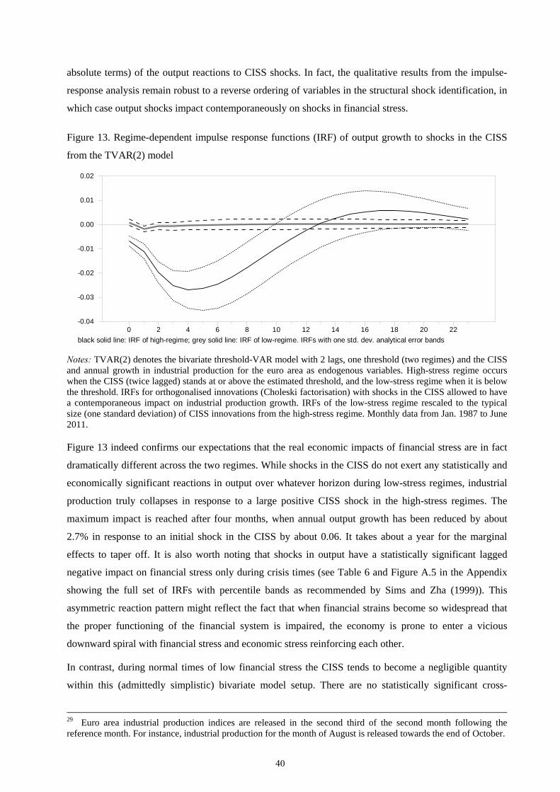
absolute terms) of the output reactions to CISS shocks. In fact, the qualitative results from the impulse-

response analysis remain robust to a reverse ordering of variables in the structural shock identification, in

which case output shocks impact contemporaneously on shocks in financial stress.

Figure 13. Regime-dependent impulse response functions (IRF) of output growth to shocks in the CISS

from the TVAR(2) model

black solid line: IRF of high-regime; grey solid line: IRF of low-regime. IRFs with one std. dev. analytical error bands

0 2 4 6 8 10 12 14 16 18 20 22-0.04

-0.03

-0.02

-0.01

0.00

0.01

0.02

Notes: TVAR(2) denotes the bivariate threshold-VAR model with 2 lags, one threshold (two regimes) and the CISS and annual growth in industrial production for the euro area as endogenous variables. High-stress regime occurs when the CISS (twice lagged) stands at or above the estimated threshold, and the low-stress regime when it is below the threshold. IRFs for orthogonalised innovations (Choleski factorisation) with shocks in the CISS allowed to have a contemporaneous impact on industrial production growth. IRFs of the low-stress regime rescaled to the typical size (one standard deviation) of CISS innovations from the high-stress regime. Monthly data from Jan. 1987 to June 2011.

Figure 13 indeed confirms our expectations that the real economic impacts of financial stress are in fact

dramatically different across the two regimes. While shocks in the CISS do not exert any statistically and

economically significant reactions in output over whatever horizon during low-stress regimes, industrial

production truly collapses in response to a large positive CISS shock in the high-stress regimes. The

maximum impact is reached after four months, when annual output growth has been reduced by about

2.7% in response to an initial shock in the CISS by about 0.06. It takes about a year for the marginal

effects to taper off. It is also worth noting that shocks in output have a statistically significant lagged

negative impact on financial stress only during crisis times (see Table 6 and Figure A.5 in the Appendix

showing the full set of IRFs with percentile bands as recommended by Sims and Zha (1999)). This

asymmetric reaction pattern might reflect the fact that when financial strains become so widespread that

the proper functioning of the financial system is impaired, the economy is prone to enter a vicious

downward spiral with financial stress and economic stress reinforcing each other.

In contrast, during normal times of low financial stress the CISS tends to become a negligible quantity

within this (admittedly simplistic) bivariate model setup. There are no statistically significant cross-

29 Euro area industrial production indices are released in the second third of the second month following the reference month. For instance, industrial production for the month of August is released towards the end of October.

40

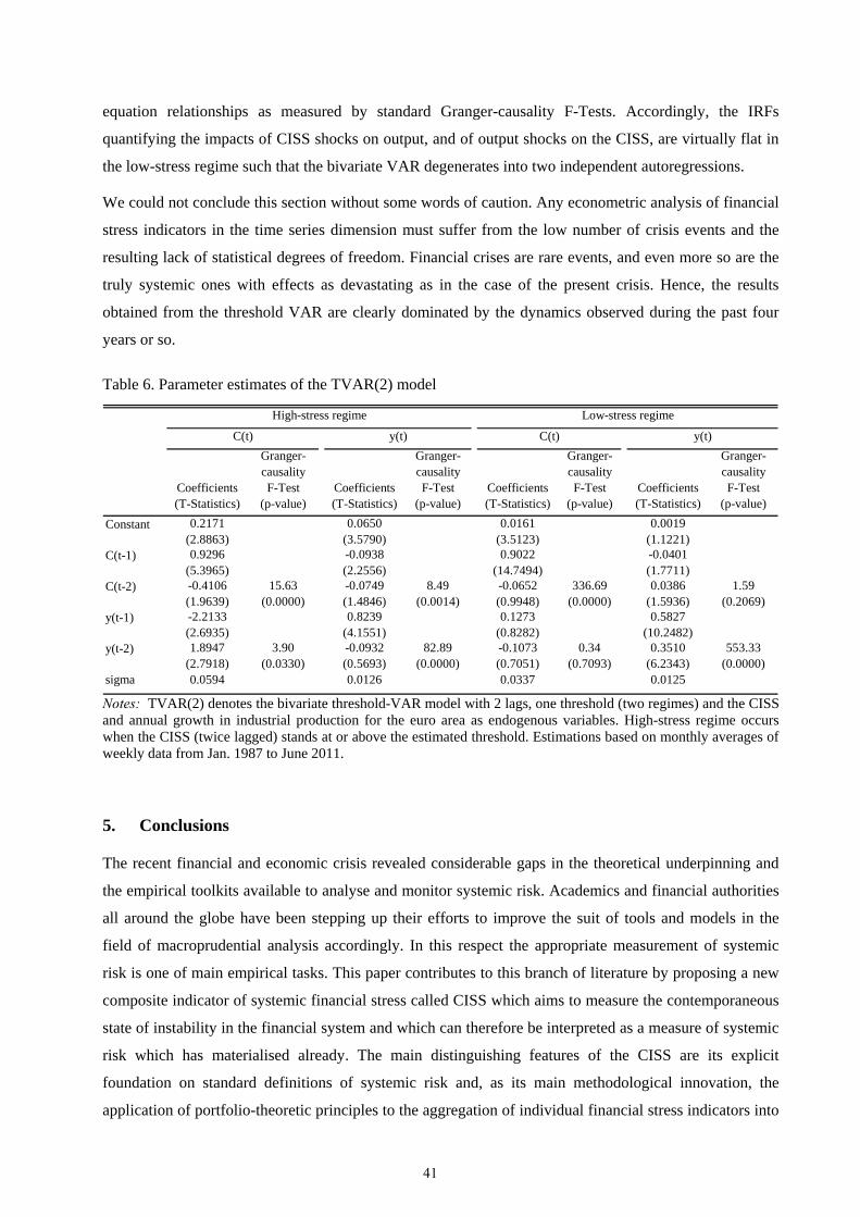
equation relationships as measured by standard Granger-causality F-Tests. Accordingly, the IRFs

quantifying the impacts of CISS shocks on output, and of output shocks on the CISS, are virtually flat in

the low-stress regime such that the bivariate VAR degenerates into two independent autoregressions.

We could not conclude this section without some words of caution. Any econometric analysis of financial

stress indicators in the time series dimension must suffer from the low number of crisis events and the

resulting lack of statistical degrees of freedom. Financial crises are rare events, and even more so are the

truly systemic ones with effects as devastating as in the case of the present crisis. Hence, the results

obtained from the threshold VAR are clearly dominated by the dynamics observed during the past four

years or so.

Table 6. Parameter estimates of the TVAR(2) model

Coefficients(T-Statistics)

Granger-causalityF-Test

(p-value)Coefficients(T-Statistics)

Granger-causalityF-Test

(p-value)Coefficients(T-Statistics)

Granger-causalityF-Test

(p-value)Coefficients(T-Statistics)

Granger-causalityF-Test

(p-value)

Constant 0.2171 (2.8863)

0.0650(3.5790)

0.0161(3.5123)

0.0019(1.1221)

C(t-1) 0.9296(5.3965)

-0.0938(2.2556)

0.9022(14.7494)

-0.0401(1.7711)

C(t-2) -0.4106(1.9639)

15.63(0.0000)

-0.0749(1.4846)

8.49(0.0014)

-0.0652(0.9948)

336.69(0.0000)

0.0386(1.5936)

1.59(0.2069)

y(t-1) -2.2133(2.6935)

0.8239(4.1551)

0.1273(0.8282)

0.5827(10.2482)

y(t-2) 1.8947(2.7918)

3.90(0.0330)

-0.0932(0.5693)

82.89(0.0000)

-0.1073(0.7051)

0.34(0.7093)

0.3510(6.2343)

553.33(0.0000)

sigma 0.0594 0.0126 0.0337 0.0125

C(t) y(t)

High-stress regime Low-stress regime

C(t) y(t)

Notes: TVAR(2) denotes the bivariate threshold-VAR model with 2 lags, one threshold (two regimes) and the CISS and annual growth in industrial production for the euro area as endogenous variables. High-stress regime occurs when the CISS (twice lagged) stands at or above the estimated threshold. Estimations based on monthly averages of weekly data from Jan. 1987 to June 2011.

5. Conclusions

The recent financial and economic crisis revealed considerable gaps in the theoretical underpinning and

the empirical toolkits available to analyse and monitor systemic risk. Academics and financial authorities

all around the globe have been stepping up their efforts to improve the suit of tools and models in the

field of macroprudential analysis accordingly. In this respect the appropriate measurement of systemic

risk is one of main empirical tasks. This paper contributes to this branch of literature by proposing a new

composite indicator of systemic financial stress called CISS which aims to measure the contemporaneous

state of instability in the financial system and which can therefore be interpreted as a measure of systemic

risk which has materialised already. The main distinguishing features of the CISS are its explicit

foundation on standard definitions of systemic risk and, as its main methodological innovation, the

application of portfolio-theoretic principles to the aggregation of individual financial stress indicators into

41

the composite indicator. We have also proposed new ways to determine critical levels (i.e., crisis

thresholds and regimes) for composite financial stress indices as the endogenous outcome of two variants

of econometric regime-switching models. The CISS can be updated quickly on a weekly and thus almost

real time basis. Its statistical robustness to computation over expanding samples ensures that past signals

issued by the CISS remain valid also at later points in time. The CISS is thus particularly suited for the

real time monitoring of the overall level of frictions and tensions in the financial system as typically done

in central banks and other macroprudential authorities.

As to the way forward, several tasks can be envisaged. An expansion of the geographical coverage of the

CISS promises to lead to a better understanding and assessment of its indicator properties. Based on the

experience from other countries the current composition of the euro area CISS could be revisited (“CISS

2.0”). In addition, the geographical expansion might also help improve the econometric analysis of the

CISS by exploiting the cross-country dimension. In a time series context, the aggregate effects of

financial stress in a single country can be more thoroughly and robustly investigated by including the

CISS in regime-switching VAR models along with a broader set of macroeconomic aggregates like in

Hartmann et al. (2012) for the euro area and in Hubrich and Tetlow (2010) for the United States based on

a different financial stress index.

References

Acharya, V. V. and D. Skeie (2011): “A Model of Liquidity Hoarding and Term Premia in Inter-bank

Markets”, CEPR Discussion Paper No. 8705, December.

Ang, A. and G. Bekaert (2002): “Regime Switches in Interest Rates”, Journal of Business and Economic

Statistics, Vol. 20, No. 2, pp. 163-182.

Baele, L. (2005): “Volatility Spillover Effects in European Equity Markets”, Journal of Financial and

Quantitative Analysis, Vol. 40, No. 2, pp. 373-401.

Baele, L., G. Bekaert and K. Inghelbrecht (2010): “The Determinants of Stock and Bond Return

Comovements”, Review of Financial Studies, Vol. 23, No. 6, pp. 2374-2428.

Bekaert, G., C. A. Harvey and A. Ng (2005): “Market Integration and Contagion”, Journal of Business,

Vol. 78, No. 1, pp. 39-69.

Bernanke, B. S., M. Gertler and S. Gilchrist (1999): “The Financial Accelerator in a Quantitative

Business Cycle Framework”, in J. Taylor and M. Woodford (eds.), Handbook of Macroeconomics,

Vol. 1, Part 3, Elsevier, pp. 1341-1393.

Billio, M., M. Getmansky, A.W. Lo and L. Pelizzon (2011): “Econometric Measures of Systemic Risk in

the Finance and Insurance Sectors”, Mimeo.

Blix Grimaldi, M. (2010): “Detecting and Interpreting Financial Stress in the Euro Area”, ECB Working

Paper Series No. 1214, June.

42

Bloom, N. (2009): “The Impact of Uncertainty Shocks”, Econometrica, Vol. 77, No. 3, pp. 623-685.

Brave, S. and R. A. Butters (2011a): “Monitoring Financial Stability: A Financial Conditions Index

Approach”, Federal Reserve Bank of Chicago, Economic Perspectives, First Quarter, pp. 22-43.

Brave, S. and R. A. Butters (2011b): “Gathering Insights on the Forest from the Trees: A New Metric for

Financial Conditions”, Mimeo, May.

Brunnermeier, M. (2009): “Deciphering the Liquidity and Credit Crunch 2007–08”, Journal of Economic

Perspectives, Vol. 23, No. 1, pp. 77–100.

Brunnermeier, M. and L. Pedersen (2009): “Market Liquidity and Funding Liquidity”, Review of

Financial Studies, Vol. 22, No. 6, pp. 2201–2238.

Caballero, R. J. and A. Krishnamurthy (2008): “Collective Risk Management in a Flight to Quality

Episode”, Journal of Finance, Vol. 63, No. 5, pp. 2195-2230.

Caldarelli, R., S. A. Elekdag and S. Lall (2011): “Financial Stress and Economic Contractions”, Journal

of Financial Stability, Vol. 7, pp. 78-97.

Carlson, M. A., T. King and K. Lewis (2011): “Distress in the Financial Sector and Economic Activity”,

B.E. Journal of Economic Analysis & Policy, Vol. 11, No. 1, Art. 35.

Chordia, T., A. Sarkar and A. Subrahmanyam (2005): “An Empirical Analysis of Stock and Bond Market

Liquidity”, Review of Financial Studies, Vol. 18, No. 1, pp. 85-129.

Coudert, V. and M. Gex (2008), “Does Risk Aversion Drive Financial Crises? Testing the Predictive

Power of Empirical Indicators”, Journal of Empirical Finance, Vol. 15, pp. 167-184.

Cuthbertson, K. and D. Nitzsche (2004), “Quantitative Financial Economics: Stocks, Bonds and Foreign

Exchange”, 2nd edition, Wiley.

Davig, T. and C. Hakkio (2010): “What is the Effect of Financial Stress on Economic Activity?”, Federal

Reserve Bank of Kansas City, Economic Review, Second Quarter, pp. 35-62.

De Bandt, O. and P. Hartmann (2000), “Systemic Risk: A Survey”, ECB Working Paper Series No. 35,

November.

De Bandt, O., P. Hartmann and J.-L. Peydro (2009), “Systemic Risk in Banking: An Update”, in A.

Berger, P. Molyneux and J. Wilson (eds.), Oxford Handbook of Banking, Oxford University Press.

Domanski, D. and M. Kremer (2000): “The Dynamics of International Asset Price Linkages and their

Effects on German Stock and Bond Markets”, Bank for International Settlements, Conference

Papers No. 8, pp. 134-158.

Doornik, J. A. (2011), “Markov-Switching Models”, University of Oxford and OxMetrics Technologies

Ltd., Mimeo.

Durlauf, S. N. and P. A. Johnson (1995): “Multiple Regimes and Cross-Country Growth Behavior”,

Journal of Applied Econometrics, Vol. 10, pp. 365-384.

43

European Central Bank (2009a), “Box 1: A Global Index of Financial Turbulence”, Financial Stability

Review, December, pp. 21-23.

European Central Bank (2009b), “Special Feature B: The Concept of Systemic Risk”, Financial Stability

Review, December, pp. 134-142.

European Central Bank (2010), “Special Feature B: Analytical Models and Tools for the Identification

and Assessment of Systemic Risks”, Financial Stability Review, June, pp. 138-146.

European Central Bank (2011), “Special Feature C: “Systemic risk methodologies”, Financial Stability

Review, June, pp. 141-148.

Feldhütter, P. and D. Lando (2008): “Decomposing Swap Spreads”, Journal of Financial Economics, Vol.

88, No. 2, pp. 375-405.

Fostel, A. and J. Geneakoplos (2008): “Leverage Cycles and the Anxious Economy”, American

Economic Review, Vol. 98, No. 4, pp. 1211-1244.

Franses, P. H. and D. van Dijk (2000): “Non-Linear Time Series Models in Empirical Finance”,

Cambridge University Press, Cambridge.

González-Rivera, Lee and Yoldas (2007): “Optimality of the RiskMetrics VaR Model”, Mimeo.

Hakkio, S. C. and W. R. Keeton (2009): “Financial Stress: What Is It, How Can It be Measured, and Why

Does It Matter?”, Federal Reserve Bank of Kansas City, Economic Review, Second Quarter, pp. 5-

50.

Hamilton, J. D. (1994): “Time Series Analaysis”, Princeton University Press, Princeton, New Jersey.

Hansen, B. E. (2000): “Sample Splitting and Threshold Estimation”, Econometrica, Vol. 68, No. 3, pp.

575-603.

Hartmann, P., K. Hubrich, M. Kremer and R. J. Tetlow (2012): “Widespread Instabilities and the

Macroeconomy - Regime Switching in the Euro Area”, European Central Bank and Federal Reserve

Board, Mimeo.

Hatzius, J., P. Hooper, F. Mishkin, K. L. Schoenholtz and M. W. Watson (2010): “Financial Conditions

Indexes: A New Look after the Financial Crisis”, NBER Working Paper 16150, July.

Heider, F., M. Hoerova and C. Holthausen (2009): “Liquidity Hoarding and Interbank Market Spreads:

The Role of Counterparty Risk, European Banking Center Discussion Paper No. 2009-11S.

Hubrich, K. and R. J. Tetlow (2010): “Financial Stress and Economic Dynamics: The Transmission of

Crises”, European Central Bank, Federal Reserve Board and IMF, Mimeo.

Illing, M. and Y. Liu (2006): “Measuring Financial Stress in a Developed Country: an Application to

Canada”, Journal of Financial Stability, Vol. 2, No. 4, pp. 243-265.

44

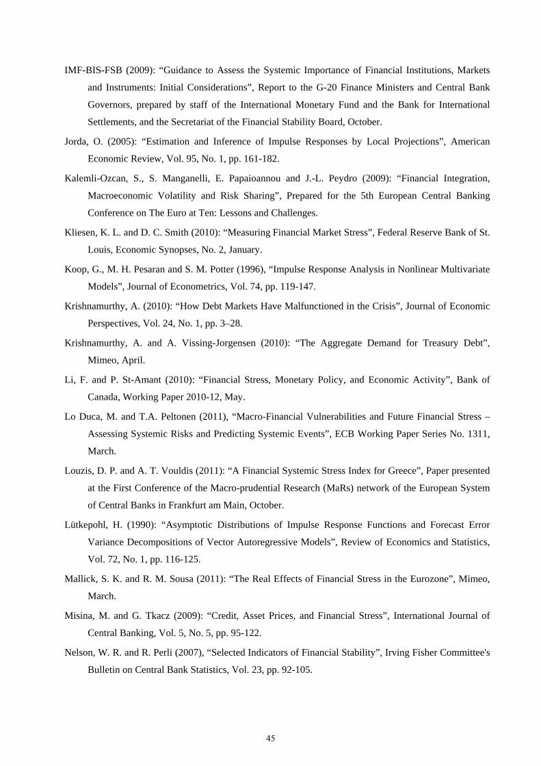
IMF-BIS-FSB (2009): “Guidance to Assess the Systemic Importance of Financial Institutions, Markets

and Instruments: Initial Considerations”, Report to the G-20 Finance Ministers and Central Bank

Governors, prepared by staff of the International Monetary Fund and the Bank for International

Settlements, and the Secretariat of the Financial Stability Board, October.

Jorda, O. (2005): “Estimation and Inference of Impulse Responses by Local Projections”, American

Economic Review, Vol. 95, No. 1, pp. 161-182.

Kalemli-Ozcan, S., S. Manganelli, E. Papaioannou and J.-L. Peydro (2009): “Financial Integration,

Macroeconomic Volatility and Risk Sharing”, Prepared for the 5th European Central Banking

Conference on The Euro at Ten: Lessons and Challenges.

Kliesen, K. L. and D. C. Smith (2010): “Measuring Financial Market Stress”, Federal Reserve Bank of St.

Louis, Economic Synopses, No. 2, January.

Koop, G., M. H. Pesaran and S. M. Potter (1996), “Impulse Response Analysis in Nonlinear Multivariate

Models”, Journal of Econometrics, Vol. 74, pp. 119-147.

Krishnamurthy, A. (2010): “How Debt Markets Have Malfunctioned in the Crisis”, Journal of Economic

Perspectives, Vol. 24, No. 1, pp. 3–28.

Krishnamurthy, A. and A. Vissing-Jorgensen (2010): “The Aggregate Demand for Treasury Debt”,

Mimeo, April.

Li, F. and P. St-Amant (2010): “Financial Stress, Monetary Policy, and Economic Activity”, Bank of

Canada, Working Paper 2010-12, May.

Lo Duca, M. and T.A. Peltonen (2011), “Macro-Financial Vulnerabilities and Future Financial Stress –

Assessing Systemic Risks and Predicting Systemic Events”, ECB Working Paper Series No. 1311,

March.

Louzis, D. P. and A. T. Vouldis (2011): “A Financial Systemic Stress Index for Greece”, Paper presented

at the First Conference of the Macro-prudential Research (MaRs) network of the European System

of Central Banks in Frankfurt am Main, October.

Lütkepohl, H. (1990): “Asymptotic Distributions of Impulse Response Functions and Forecast Error

Variance Decompositions of Vector Autoregressive Models”, Review of Economics and Statistics,

Vol. 72, No. 1, pp. 116-125.

Mallick, S. K. and R. M. Sousa (2011): “The Real Effects of Financial Stress in the Eurozone”, Mimeo,

March.

Misina, M. and G. Tkacz (2009): “Credit, Asset Prices, and Financial Stress”, International Journal of

Central Banking, Vol. 5, No. 5, pp. 95-122.

Nelson, W. R. and R. Perli (2007), “Selected Indicators of Financial Stability”, Irving Fisher Committee's

Bulletin on Central Bank Statistics, Vol. 23, pp. 92-105.

45

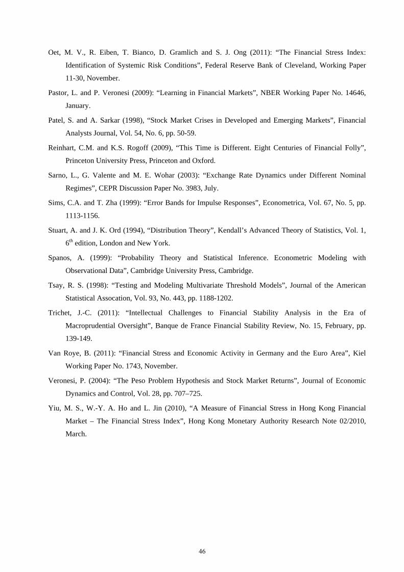
Oet, M. V., R. Eiben, T. Bianco, D. Gramlich and S. J. Ong (2011): “The Financial Stress Index:

Identification of Systemic Risk Conditions”, Federal Reserve Bank of Cleveland, Working Paper

11-30, November.

Pastor, L. and P. Veronesi (2009): “Learning in Financial Markets”, NBER Working Paper No. 14646,

January.

Patel, S. and A. Sarkar (1998), “Stock Market Crises in Developed and Emerging Markets”, Financial

Analysts Journal, Vol. 54, No. 6, pp. 50-59.

Reinhart, C.M. and K.S. Rogoff (2009), “This Time is Different. Eight Centuries of Financial Folly”,

Princeton University Press, Princeton and Oxford.

Sarno, L., G. Valente and M. E. Wohar (2003): “Exchange Rate Dynamics under Different Nominal

Regimes”, CEPR Discussion Paper No. 3983, July.

Sims, C.A. and T. Zha (1999): “Error Bands for Impulse Responses”, Econometrica, Vol. 67, No. 5, pp.

1113-1156.

Stuart, A. and J. K. Ord (1994), “Distribution Theory”, Kendall’s Advanced Theory of Statistics, Vol. 1,

6th edition, London and New York.

Spanos, A. (1999): “Probability Theory and Statistical Inference. Econometric Modeling with

Observational Data”, Cambridge University Press, Cambridge.

Tsay, R. S. (1998): “Testing and Modeling Multivariate Threshold Models”, Journal of the American

Statistical Assocation, Vol. 93, No. 443, pp. 1188-1202.

Trichet, J.-C. (2011): “Intellectual Challenges to Financial Stability Analysis in the Era of

Macroprudential Oversight”, Banque de France Financial Stability Review, No. 15, February, pp.

139-149.

Van Roye, B. (2011): “Financial Stress and Economic Activity in Germany and the Euro Area”, Kiel

Working Paper No. 1743, November.

Veronesi, P. (2004): “The Peso Problem Hypothesis and Stock Market Returns”, Journal of Economic

Dynamics and Control, Vol. 28, pp. 707–725.

Yiu, M. S., W.-Y. A. Ho and L. Jin (2010), “A Measure of Financial Stress in Hong Kong Financial

Market – The Financial Stress Index”, Hong Kong Monetary Authority Research Note 02/2010,

March.

46

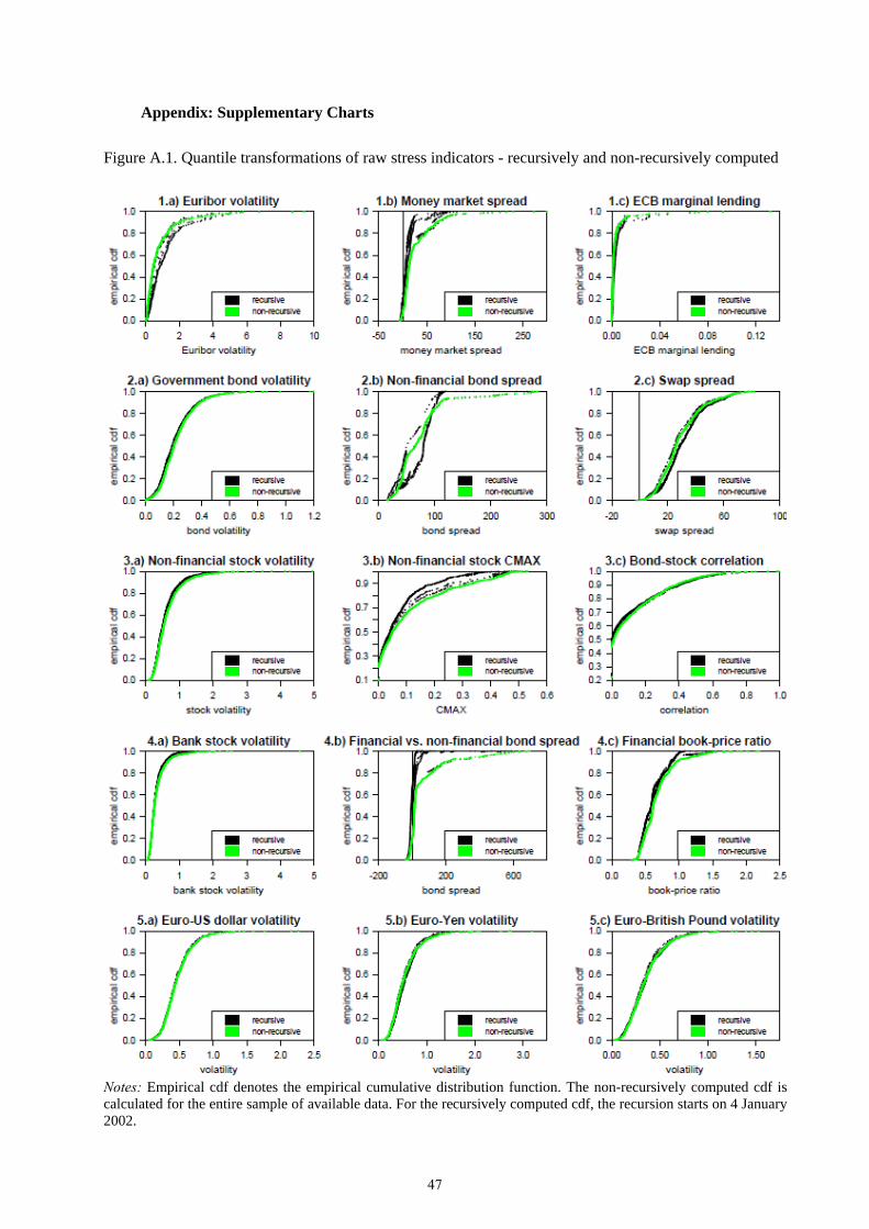
Appendix: Supplementary Charts

Figure A.1. Quantile transformations of raw stress indicators - recursively and non-recursively computed

Notes: Empirical cdf denotes the empirical cumulative distribution function. The non-recursively computed cdf is calculated for the entire sample of available data. For the recursively computed cdf, the recursion starts on 4 January 2002.

47

Figure A.2. CISS computed with different subindex weights

1987 1989 1991 1993 1995 1997 1999 2001 2003 2005 2007 2009 20110.00

0.25

0.50

0.75

1.00CISS imp. weight

CISS eq. weights

Notes: CISS computed for two different sets of subindex weights: “real-impact weights” (money market: 15%, bond market: 15%, equity market: 25%, financial intermediaries: 30%, and foreign exchange market: 15%, see section 3.4), and “equal weights” (with 20% weight assigned to each subindex). Weekly euro area data from 8 Jan. 1999 to 24 June 2011.

Figure A.3. Decomposition of the CISS

money market

bond market

equity market

financials

forex

correlations

CISS

1999 2000 2001 2002 2003 2004 2005 2006 2007 2008 2009 2010 2011-0.50

-0.25

0.00

0.25

0.50

0.75

1.00

-0.50

-0.25

0.00

0.25

0.50

0.75

1.00

Notes: This figure shows the decomposition of the CISS into contributions from each subindex (with real-impact weights) and from all cross-correlations jointly (calculated as the difference between the proper CISS and the squared weighted average of subindices). Weekly euro area data from 8 Jan. 1999 to 24 June 2011.

48

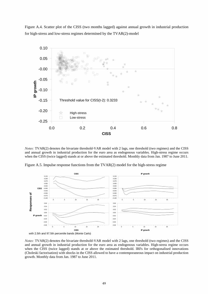
Figure A.4. Scatter plot of the CISS (two months lagged) against annual growth in industrial production

for high-stress and low-stress regimes determined by the TVAR(2)-model

CISS

IP g

row

th

0.0 0.2 0.4 0.6 0.8

-0.25

-0.20

-0.15

-0.10

-0.05

-0.00

0.05

0.10

High-stress

Low-stress

Threshold value for CISS(t-2): 0.3233

Notes: TVAR(2) denotes the bivariate threshold-VAR model with 2 lags, one threshold (two regimes) and the CISS and annual growth in industrial production for the euro area as endogenous variables. High-stress regime occurs when the CISS (twice lagged) stands at or above the estimated threshold. Monthly data from Jan. 1987 to June 2011.

Figure A.5. Impulse response functions from the TVAR(2) model for the high-stress regime

with 2.5th and 97.5th percentile bands (Monte Carlo)

Res

po

nse

s o

f

CISS

IP growth

CISS

CISS

IP growth

IP growth

0 5 10 15 20-0.100

-0.075

-0.050

-0.025

-0.000

0.025

0.050

0.075

0.100

0.125

0 5 10 15 20-0.100

-0.075

-0.050

-0.025

-0.000

0.025

0.050

0.075

0.100

0.125

0 5 10 15 20-0.08

-0.06

-0.04

-0.02

0.00

0.02

0.04

0.06

0 5 10 15 20-0.08

-0.06

-0.04

-0.02

0.00

0.02

0.04

0.06

Notes: TVAR(2) denotes the bivariate threshold-VAR model with 2 lags, one threshold (two regimes) and the CISS and annual growth in industrial production for the euro area as endogenous variables. High-stress regime occurs when the CISS (twice lagged) stands at or above the estimated threshold. IRFs for orthogonalised innovations (Choleski factorisation) with shocks in the CISS allowed to have a contemporaneous impact on industrial production growth. Monthly data from Jan. 1987 to June 2011.

49