Bank of Canada Banque du Canada

Working Paper 2000-3 / Document de travail 2000-3

Long-Term Determinants of the Personal Savings Rate:Literature Review and Some Empirical Results for Canada

by

Gilles Bérubé and Denise Côté

ISSN 1192-5434ISBN 0-662-28581-6Cat. FB3-2/100-3E

Printed in Canada on recycled paper

Bank of Canada Working Paper 2000-3

February 2000

Long-Term Determinants of the Personal Savings Rate:Literature Review and Some Empirical Results for Canada

byGilles Bérubé and Denise Côté

Research DepartmentBank of Canada

Ottawa, Canada K1A 0G9dcote@bank-banque-canada.ca

The views expressed in this paper are those of the authors.No responsibility for them should be attributed to the Bank of Canada.

iii

.....

...

.....

......

.....

........12

.......

...

......18

......24

.....25

...

..

......49

........51

Contents

Acknowledgements............................................................................................................ iv

Abstract/Résumé....................................................................................................................v

1. Introduction...............................................................................................................................1

2. Literature review.......................................................................................................................3

2.1 Demographics...............................................................................................................5

2.2 The real rate of return ..................................................................................................7

2.3 Liquidity constraints...................................................................................................10

2.4 Inflation............................................................................................................................11

2.5 Government fiscal balances .....................................................................................

2.6 Public pension plans .................................................................................................13

2.7 Private wealth ...............................................................................................................15

3. Empirical analysis...................................................................................................................16

3.1 Estimating the long-run parameters of the National Income and Expenditure

Accounts (NIEA) savings rate...................................................................................

3.2 Estimating the long-run parameters of the National Balance Sheet Accounts

(NBSA) savings rate..................................................................................................

3.3 Empirical interpretation of the trend NIEA savings rate............................................

4. Conclusions.............................................................................................................................27

Tables ..........................................................................................................................29

Figures ...........................................................................................................................39

Appendix 1: Description of the data.................................................................................

Appendix 2: Two measures of the personal savings rate................................................

Bibliography ...........................................................................................................................53

iv

on,

ike to

diting

Acknowledgements

The authors would like to thank Irene Ip, David Longworth, Tiff Macklem, Stephen Murchis

Brian O’Reilly, and Gerald Stuber for comments and suggestions. The authors would also l

thank Richard Lacroix for his assistance in preparing the graphs and Patricia Buchanan for e

the paper.

v

ver the

t rate,

tio of

of the

counts

ecent

nsitory

scal

ing a

ersonal

ed by

sonal

is not

rels de

nnées.

olde

ages à

taux

es. Selon

depuis

ielle du

actuel,

it que

ôt une

e des

sont

Abstract

This paper examines the structural determinants of the personal savings rate in Canada o

last 30 years, using cointegration techniques. The main finding is that the real interes

expected inflation, the ratio of the all-government fiscal balances to nominal GDP, and the ra

household net worth to personal disposable income are the most important determinants

trend in the personal savings rate, as measured in the National Income and Expenditure Ac

(NIEA). The results also suggest that the rapid decline in the NIEA personal savings rate in r

years largely reflects a change in the trend component of the savings rate, rather than a tra

departure from the trend. In the current environment of low inflation and government fi

balances moving into surpluses, the trend NIEA savings rate could remain low. When us

measure of the personal savings rate based on the change in the net worth position of the p

sector (as estimated in the National Balance Sheet Accounts [NBSA]), the trend is determin

the real interest rate, expected inflation, and the ratio of household net worth to per

disposable income. However, the statistical evidence supporting this long-run relationship

as conclusive as that for the NIEA savings rate.

JEL classifications: C22, E21

Bank classifications: Domestic demand and components

Résumé

Au moyen de techniques de cointégration, les auteurs étudient les déterminants structu

l’évolution du taux d’épargne des particuliers au Canada au cours des trente dernières a

Leur principale conclusion est que le taux d’intérêt réel, l’inflation attendue, le ratio du s

budgétaire de l’ensemble du secteur public au PIB nominal et le ratio de l’avoir net des mén

leur revenu disponible constituent les principaux déterminants de l’évolution à long terme du

d’épargne des particuliers mesuré dans les comptes nationaux des revenus et des dépens

les résultats obtenus par les auteurs, la baisse rapide que ce taux d’épargne connaît

quelques années refléterait essentiellement une modification de la composante tendanc

taux d’épargne plutôt qu’un écart transitoire par rapport à la tendance. Dans le contexte

caractérisé par un bas taux d’inflation et l’apparition d’excédents budgétaires, il se pourra

cette mesure du taux d’épargne tendanciel demeure faible. Si les auteurs utilisent plut

mesure fondée sur la variation de l’avoir net du secteur des particuliers (estimée à l’aid

comptes du bilan national), les déterminants de l’évolution tendancielle du taux d’épargne

vi

venu

me ne

ationaux

alors le taux d’intérêt réel, l’inflation attendue et le ratio de l’avoir net des ménages à leur re

disponible. Toutefois, les résultats statistiques obtenus à l’appui de cette relation à long ter

sont pas aussi concluants que dans le cas du taux d’épargne mesuré dans les comptes n

des revenus et des dépenses.

Classifications JEL : C22, E21

Classification de la Banque : Demande intérieure et composantes

1

emand

is an

Income

w of

umption

yzing

ot take

s do not

cern of

erated

rsonal

e, and

s. The

Capital

o not

es in

s are not

m

ture

fits are

part of

lance

retical

values,

flation

tion of

he most

1. Introduction

Savings play a central role in income determination, both in the short run through aggregate d

and in the long run through capital formation and wealth accumulation. Personal savings

important source of national savings (see Table 1 and Figure 1).1 Since the early 1980s, the

conventional measure of the personal savings rate in Canada, as calculated in the National

and Expenditure Accounts (NIEA), has been trending downwards. It reached an all-time lo

2.3 per cent in 1998. These developments have raised concerns that recent household cons

levels may not be sustainable.

Many analysts argue that the NIEA measure of personal savings is not reliable for anal

and forecasting households’ consumption behaviour because, among other things, it does n

into account changes in asset values such as capital gains or losses. Those gains or losse

affect measured income but they can have an impact on consumption. However, the main con

the NIEA is to provide estimates of the production of goods and services and the income gen

by those processes. Within that framework, personal savings is derived by first estimating pe

income, then subtracting current transfers to government to obtain personal disposable incom

then subtracting consumption and current transfers to corporations and to non-resident

savings rate is what is left over, expressed as a percentage of personal disposable income.

gains or losses are not included in the NIEA definition of savings on the basis that they d

represent added value, generated by the production process.

Even if one accepts the NIEA definition of savings, there still remain some asymmetri

the way income and taxes are treated. For instance, even though the changes in asset value

counted as investment income, taxes onrealizedcapital gains (or losses) are still subtracted fro

current income in the NIEA definition. Also, interest earned on accumulation of rights to fu

pensions is recorded as investment income but no tax is paid on that income until the bene

drawn down. Thus, the NIEA measure does not take into account trusteed pension benefits as

current income although it records taxes on those same benefits.

The change in the net worth of the personal sector, as estimated in the National Ba

Sheet Accounts (NBSA), provides an alternative measure of savings that is closer to the theo

concept. For instance, the NBSA estimates of household savings reflect changes in asset

include the stock of consumer durables in personal assets, and are not affected by the in

premium in asset returns. The change in the net worth of the personal sector, as a propor

1. Personal savings as a share of nominal GDP has decreased since the early 1980s but remained timportant source of national savings up to, and including, 1995.

2

re, the

lly low

vel of

risk for

ent of

. Is the

hould

erlying

-term

sis is

based

urement

[1998]

omic

rate of

ving/

h the

xpected

tio of

e trend

ted by

g-run

mixed

ich we

avings

rate.

lances

.

personal disposable income, is normally much higher than the NIEA savings ratio. Furthermo

most recent values of this alternative measure of the personal savings rate are not unusua

relative to their average of the last five years or so. This may suggest that the current le

personal savings does not present, as some analysts suggest, a substantial negative

household demand in the near term.

However, there still remains a problem with this kind of analysis: there is no assessm

the level of the savings ratio that one would expect to observe based on fundamental factors

observed ratio higher or lower than what would be consistent with the fundamentals? Where s

we expect the trend personal savings rate to go in the coming years, based on the und

fundamentals?

The objective of the present paper is to answer these questions by identifying the long

determinants of the personal savings rate, using cointegration techniques. Our analy

performed for both the NIEA measure of the personal savings rate and the alternative NBSA-

measure. However, it should be emphasized that our paper does not deal per se with meas

issues that are currently at the centre of the savings rate discussion in Canada. (See Coiteux

and Appendix 2 at the end of this paper for an overview on measurement issues.)

We consider in our analysis a number of factors that have been identified in the econ

literature as potential determinants of personal savings. These include demographics, the

return on savings, liquidity constraints, private wealth, public pension plans, government sa

dissaving, and uncertainty about future income growth. We begin our empirical analysis wit

NIEA measure of the personal savings rate. Our results suggest that the real interest rate, e

inflation, the all-government fiscal balances as a proportion of nominal GDP, and the ra

household net worth to personal disposable income are the most important determinants of th

in this measure of the personal savings rate over the 1965–96 period. This finding is suppor

formal statistical tests for cointegration. However, although our best equation captures lon

movement in the NIEA savings rate quite well, there remain some problems, such as the

evidence of long-run stability between the savings rate and the above structural factors, wh

suspect may be due to the variable used to measure expected inflation.

The results also suggest that the rapid decline in the NIEA measure of the personal s

rate in recent years is essentially attributable to the trend component of the savings

Furthermore, based on current projections for the inflation rate and government fiscal ba

moving into surpluses, the trend NIEA measure of the personal savings rate could remain low

3

orth of

end is

rth to

nship

irical

sider in

inants.

savings

of the

sets to

ut the

ition of

idered

ption

ing

d base

ate of

orrow

main

from

riod,

the

poral

me is

els of

life-

When using a measure of the personal savings rate based on the change in the net w

the personal sector (as estimated in the National Balance Sheet Accounts [NBSA]), the tr

determined by the real interest rate, expected inflation, and the ratio of household net wo

personal disposable income. However, the statistical evidence supporting this long-run relatio

is not as conclusive as that for the NIEA savings rate.

The plan of the paper is as follows. Section 2 surveys the existing theoretical and emp

literature on the structural determinants of the aggregate personal savings rate that we con

our empirical work and describes the specific variables that we use to represent these determ

Section 3 examines the long-run relationships between the two measures of the personal

rate and the variables identified in Section 2, using cointegration techniques. The final section

paper summarizes our main results and comments on future research.

2. Literature review

Personal savings decisions are driven by several motives, including the need to build up as

finance consumption after retirement, precautionary saving related to the uncertainty abo

future, the desire to leave bequests to a subsequent generation, and saving for the acquis

tangible assets or for large current expenditures. Saving for retirement is generally cons

quantitatively the most important saving motive. Much of the analysis of households’ consum

and savings decisions is conducted using versions of the life-cycle model.

In the basic life-cycle model, the motivation for saving is providing for consumption dur

retirement years. Simple versions of this model assume that individuals are far-sighted an

their decisions on future events (income, interest rate, family composition, rate of survival, d

death) that are known with certainty. Capital markets are perfect, so that individuals can b

against their future income to finance current consumption. As a result, one of the

implications of the life-cycle model is that individuals can separate their consumption profile

their income profile; that is, consumption is not affected by the timing of income. In any one pe

an individual’s consumption is constrained only by her/his lifetime resources.2

In order to equalize the discounted marginal utility of consumption from one period to

next, optimizing households aim to achieve a smooth level of consumption over time. Intertem

consumption smoothing is achieved by saving when income is high and dissaving when inco

low. Individuals tend to dissave (or borrow) when they are young, because of relatively low lev

2. See Browning and Lusardi (1996) for a theoretical discussion of the assumptions of the standardcycle model and their implications.

4

s, with

uring

lso, the

nd an

by a

uture

el are

rrow

w large

ns. By

zable

ows.

ly over

nada,

r cent

ulate

lderly

do not

unts of

for

life-

inties

tionary

ion. In

ce the

g (or

of an

or

995)ing isto

income and high expenditures related to household formation, and save in their middle year

asset holdings reaching their maximum at retirement age. Individuals dissave again d

retirement by drawing on their accumulated assets, which are entirely exhausted at death. A

life-cycle approach predicts a negative relationship between expected lifetime resources a

individual’s savings rate. For a given level of current income, the savings rate will be reduced

permanent increase in wealth, since fewer savings will be needed to provide for f

consumption.

However, several of the key assumptions and predictions of the basic life-cycle mod

not supported by empirical evidence. In practice, households face limits on their ability to bo

against future resources. For instance, marketable assets are required as collateral to borro

amounts of money, there are credit limits, and interest rates are higher on unsecured loa

preventing full intertemporal smoothing of consumption, borrowing constraints may lead a si

proportion of consumers to link consumption/savings decisions to disposable income fl

Indeed, empirical evidence suggest that consumption tracks household income quite close

the life cycle (Campbell and Mankiw 1989; Carroll and Summers 1991). In the case of Ca

Wirjanto (1995) estimates the proportion of liquidity-constrained consumers at about 46 pe

while Campbell and Mankiw (1991) estimate this proportion at about 25 per cent.

Also, most empirical evidence does not support the prediction that individuals decum

and exhaust their wealth during retirement. Rather, it appears that the savings rates of e

households are not significantly lower than those of working-age households; that the elderly

decumulate assets, or do so only slowly; and that elderly households transfer significant amo

wealth to their offspring (Carroll and Summers 1991; Kotlikoff 1988; Weil 1994).3

To account for such evidence, more recent versions of the life-cycle model allow

liquidity constraints and for imperfect markets for insurance. In these richer versions of the

cycle model, risk-averse behaviour in the presence of liquidity constraints and uncerta

regarding the length of life, earnings, medical expenses, and family support generate precau

saving, and people tend to die with positive wealth that is bequeathed to the next generat

particular, uncertainty about time of death tends to increase savings during retirement sin

elderly do not want to exhaust their wealth before they die (Davies 1981). Continuing savin

lack of dissaving) during the retirement phase of the life cycle may also reflect the working

explicit bequest motive and life planning for it, either because the utility of their children

3. Such evidence is usually obtained in studies that make use of household (micro) data. Meredith (1argues that income and wealth are often not defined appropriately in these studies, and that savinferred from hypothetically constructed wealth profiles of the elderly that may be subjectconsiderable mismeasurement problems.

5

e care

e that

olds

term

er the

ints,

nsion

in our

is by

inants

our

riately

ctors

e the

ure of

period.

regate

age. An

e the

less than

pre-

d a large

in the

rsonal

e been

ue

bequests per se enter their lifetime utility function, or owing to the use of bequests to purchas

and attention from their children. In a related paper, Banks, Blundell, and Tanner (1998) argu

the only way to fully reconcile the fall in consumption and rise in savings of retiring househ

with the life-cycle model is with the systematic arrival of unexpected adverse information.

The literature on household saving points to a number of potential important long-

determinants of the aggregate personal savings rate. In our empirical work, we consid

following structural factors: demographics, the rate of return on savings, liquidity constra

uncertainty about future income growth, inflation, government saving/dissaving, public pe

plans, and private wealth. We consider eight variables to represent these various factors

empirical work. Although this is a large number of variables to include in such an exercise, it

no means an exhaustive list of all the variables that can serve to represent the long-run determ

of the personal savings rate.4 The strength of the bequest motive, for example, is not included in

empirical work, due to the lack of indicators that could serve to represent such a factor approp

in a study using macrodata.

In the remainder of this section, we review the existing literature on the fundamental fa

of personal saving that are taken into consideration in our empirical work. We also describ

specific variables that we have selected to represent these factors in our equations.

2.1 Demographics

Demographic dimensions of particular importance in life-cycle models include the age struct

the population and the expected length of the retirement span relative to the income earning

In the basic life-cycle model, the age distribution of households has an effect on the agg

personal savings rate because the savings rates of individuals are assumed to vary with their

increase in the proportion of elderly households in the population is expected to reduc

aggregate savings rate because retired households are assumed to dissave, or at least save

those of working age. Similarly, an increase in the proportion of the population that is of

working age is also expected to reduce the aggregate personal savings rate as parents spen

proportion of their income on taking care of their children.

Most empirical studies using aggregate (macro) data have found that increases

proportions of both the youth and the elderly in the population depress the aggregate pe

savings rate, as predicted by the basic life-cycle model. Studies using cross-country data hav

4. Collinearity may increase with the number of variables, complicating the identification of a uniqcointegrating relationship.

6

ficant

ution

of a

of the

1991).

g age

ast 30

ggregate

lation

gs rate,

r the

holds

results

uch as

ds may

pected

ns for

groups,

rtant

ment

se the

savings

often

dency

of the

20 to

ment

use a

e

rsonal

more successful than studies using time-series data for individual countries in finding signi

effects of the age distribution, probably because the variation over time in the age distrib

within one country is relatively small (Masson, Bayoumi, and Samiei 1995). The impact

change in the proportion of the population represented by the elderly typically exceeds that

proportion represented by the young (Meredith 1995; Bosworth, Burtless, and Sabelhaus

Nevertheless, for a country like Canada, where the decline in the proportion of the pre-workin

population has dominated the increase in the proportion of the elderly population over the l

years, the net effect of these changes in the age structure might have been to increase the a

personal savings rate.

While studies using aggregate data show that increases in the proportion of the popu

represented by the elderly have a significant negative effect on the aggregate personal savin

studies using household (micro) data (including data for Canada) find little or no tendency fo

elderly to dissave or to save at rates markedly lower than those of working-age house

(Bosworth, Burtless, and Sabelhaus 1991). Weil (1994) suggests that these contradictory

may be reconciled by taking into account intergenerational relations between households, s

bequests, that would be picked up in aggregate data, but not in microdata. Younger househol

lower their savings rate if they expect to receive bequests (as the latter increase their ex

lifetime resources). As a result, a negative coefficient on the elderly population ratio in equatio

the aggregate personal savings rate could reflect a reduction in the savings of younger age

rather than dissaving by the elderly.

As mentioned above, the expected length of the retirement period is another impo

demographic variable in life-cycle models. Increases in the expected length of the retire

period, either through a higher life expectancy or through a decline in the retirement age, rai

need for more saving in younger ages, putting upward pressure on the aggregate personal

rate. Evidence supporting this assumption is reported in Sturm (1983).

In previous empirical work, the age structure of the population has been included more

than the length of the retirement period. In particular, these studies consider the youth-depen

ratio and the elderly-dependency ratio. The youth-dependency ratio is defined as the ratio

pre-working age population (age category 0 to 19 years) to the working-age population (aged

64). The elderly-dependency ratio is represented by the ratio of the population in the retire

phase (aged 65 and over) to the working-age population (aged 20 to 64). Several studies

“dependency ratio” variable that combines the two age groups.5 We have elected to consider th

5. This choice amounts to assuming that the net effects of each age group on the aggregate pesavings rate are identical, which is something that cannot be determineda priori.

7

er of

t of

ct on

his is

lation

st of

tting

ds to

in order

hange

er or

ebt. In

present

resent

ate to

w to a

fect of

ncome

t lender

,

fect on

r real

ue of

buttion

1998

latter demographic variable in our set of explanatory variables in order to limit the numb

variables used in the cointegration analysis.

Although the expected length of the retirement period is not included in our se

determinants, the coefficient on the ratio of the elderly population will be influenced by the effe

saving of the expectation of a longer retirement period arising from a higher life expectancy. T

so because increases in the elderly population ratio come about not only from slower popu

growth (due to lower fertility rates) but also from greater longevity.6

2.2 The real rate of return

The net result of a change in the real rate of return, i.e., a change in the opportunity co

consumption in the current period, is theoretically ambiguous because of potentially offse

substitution, income, and revaluation effects. An increase in the real rate of interest ten

encourage individuals to postpone consumption and increase savings in the present period

to achieve higher consumption levels later. That is, the intertemporal substitution effect of a c

in the real rate of interest on savings is positive.

The direction of the income effect depends on whether the individual is a net lend

borrower. A net lender receives more in investment income than he has to pay to service his d

that case, higher interest rates increase net investment income, thus encouraging

consumption and lessening the need to save in order to finance future consumption. If p

consumption and future consumption are normal goods, it is possible for a higher interest r

cause present consumption to rise, while the smaller amount of savings will nevertheless gro

larger amount of future consumption. Hence, for net lenders (net savers), the overall direct ef

an increase in the rate of return on savings behaviour is ambiguous, since substitution and i

effects act in opposite directions. Even though in the aggregate the household sector is a ne

to other sectors in the economy (i.e., net source of capital),7 the positive income effects on lenders

which may be substantially reduced by taxes, can be outweighed by the negative income ef

borrowers (Montplaisir 1997).

The real rate of interest has also another, and indirect, effect on savings. A highe

interest rate results in a fall in non-human wealth, mostly through a decline in the real val

6. Slower population growth due to lower fertility rate leaves individual savings profiles unchanged,can lead to lower aggregate savings as the proportion of the low-saving elderly in the populaincreases if the elderly have low savings rates (Sturm 1983).

7. The household sector was a net lender since the early 1970s with the exception of 1997 andduring which it was a net borrower.

8

lower

real

ected

s with

titution

tant the

rate is

of the

trated

hat the

tive of

nd no

each,

) who

er, the

te of

x real

x rate is

tax real

period

dway,

total

the rate

NIEA)

referred

reaser returngher

ct as

nsionterest

financial assets on which the interest rate is fixed for several years in advance and through

equity prices since the income flows of equities typically do not rise proportionately with the

interest rate. A higher real interest rate also results in lower human wealth as the exp

discounted value of current and future after-tax labour income and public sector transfers fall

an increase in the interest rate. The revaluation effect works in the same direction as the subs

effect, as it acts to reduce present consumption and increase saving in order to maintain cons

real value of the stock of wealth.8

The usual presumption is that the total effect on saving of a change in the real interest

positive. However, empirical research has reported mixed results with respect to the sign

direct effect of interest rates on saving. The weight of the empirical evidence, which is concen

on the United States but also includes studies for the other industrial countries, suggests t

partial correlation between the real interest rate and the savings rate is rather small, irrespec

its sign. Empirical studies focusing more particularly on Canadian data have generally fou

significant large real interest rate effects on personal saving (Burbidge and Davies 1994; B

Boadway, and Bruce 1988; Salgado and Li 1998). An exception is Thomas and Towe (1996

obtain a relatively large effect of the real interest rate on personal saving in Canada. Howev

sign of the effect is sensitive to the measure of the savings rate.9

Although what really matters for consumption/savings decisions is the after-tax real ra

return on savings, most empirical studies of personal saving (or consumption) use a pre-ta

interest rate. This is presumably done because measuring the aggregate marginal income ta

not straightforward. In the studies on the personal savings rate in Canada that use an after-

interest rate, the marginal income tax rate is usually assumed to be constant over the sample

at 30 per cent (Beach, Boadway, and Bruce 1988; Carroll and Summers 1987). Beach, Boa

and Bruce (1988) also adjust the marginal tax rate for the fraction of tax-sheltered saving to

household saving. This adjustment reflects the view that tax-deferred savings plans increase

of return to savings (at the margin) and thus contribute to increased saving.10Carroll and Summers

(1987) argue that the upward trend in the Canadian personal savings rate (as measured in the

in the 1970s and up until 1982 may have been caused by the expansion of the access to tax-p

8. Note that the presence of target savers may lessen the effect of higher rates of return to incaggregate household savings since target savers may reduce their saving in response to a higheon existing wealth. On the other hand, higher rates of return may force higher saving as himortgage services costs will reduce the amount available to pay off the principal.

9. In most studies, the coefficient on the real interest rate will be influenced by the revaluation effethe regressions do not include a human wealth variable.

10. In Canada, tax-sheltered saving includes employer/employee contributions to registered peplans, registered retirement savings plans, and registered home-ownership plans, plus tax-free inon the stock of sheltered saving.

9

tion in

in the

tered

ates of

imates

over the

each,

iduals

ressive

e effect

ltered

work

tle

nal tax

et of

of an

t as in

n the

ce for a

ost of

sists of

ears.

most

t rate

g, nototion

d theirisevingnot

ted

saving through the RRSP program. Also, Burbidge and Davies (1994) suggest that the reduc

the Canadian personal savings rate after 1982 may have been caused by a reduction

generosity of tax incentives for saving.11

A marginal income tax rate of 30 per cent, before adjustments for the fraction of shel

saving, seems rather low for Canada. For instance, the OECD has recently published estim

the marginal income tax rates for production workers in Canada in 1978 and 1995. These est

suggest that the marginal income tax rate in Canada was above 30 per cent and increasing

last 20 years or so (OECD 1998). Also, the adjustment for tax-sheltered savings made by B

Boadway, and Bruce (1988) may not be appropriate. Ragan (1994) shows that, when indiv

have access to both tax-sheltered and unsheltered saving instruments and when a prog

income tax system is in place, savings plans that defer taxable income to later years have th

of increasing future marginal income tax rates. Thus the after-tax return on marginal unshe

saving is lowered, with the result that the substitution effect of tax-deferred savings plans may

to reduce the level of saving.12 In any event, Beach, Boadway, and Bruce (1988) found lit

difference in their estimation results between assuming a zero marginal tax rate and a margi

rate of 30 per cent adjusted for the proportion of tax-sheltered savings.

Given this background, we prefer to include the pre-tax real rate of interest in our s

explanatory variables. We then test the sensitivity of the estimation results to the introduction

after-tax real rate of return, obtained by assuming a constant marginal tax rate of 30 per cen

previous studies.13 The pre-tax real rate of interest is measured as the difference betwee

interest rate on 3- to 5-year government bonds and a measure of expected inflation. The choi

3- to 5-year maturity term is based on the existing evidence for Canada, which indicates that m

interest-bearing assets and financial liabilities on the household sector’s balance sheet con

medium- and long-term fixed-rate instruments—particularly contracts with terms of 3 to 5 y

This suggests that interest rates associated with these maturities are likely to exert the

influence on household investment income and liquidity constraints. Short-term interes

11. Carroll and Summers (1987) suggest that tax-deferred saving vehicles can generate new savinbecause of the deferral of taxes, but rather because the increased availability and intensive promof such vehicles may have made consumers more aware of the benefits of saving and reshapeattitudes towards saving for retirement. A similar suggestion is made by Poterba, Venti, and W(1996), who present microeconomic evidence supporting the view that tax-deferred retirement savehicles in the United States (IRA and 401(k) plans) represent largely new saving that wouldotherwise have occurred.

12. Tax-sheltered saving may reduce non-registered saving.13. The after-tax real rate of return is calculated as follows: nominal interest rate *(1-.3) - expec

inflation.

10

t on

s in

1993;

holds to

ify for

and a

1992;

ional

ts in

umers.

in the

some of

nsumer

eilings

ive to

.

e as a

umer

before

rowing

s and

ss toeen

g thet anvings

largelyace

developments will influence consumption and savings decisions through their effec

expectations about future rates (Montplaisir 1997).

2.3 Liquidity constraints

Relative to a world with perfect capital markets, borrowing constraints increase saving

anticipation of future consumption needs that cannot be financed through credit (De Gregorio

Jappelli and Pagano 1994). For instance, down-payment requirements tend to induce house

postpone consumption early in the life cycle in order to accumulate enough assets to qual

buying a house. Also, borrowing constraints, together with uncertainty about future income

propensity towards prudence by households, generates precautionary savings (Carroll

Carroll and Samwick 1995). The inability to borrow when times are bad provides an addit

motive for accumulating assets when times are good, even for impatient consumers.

However, in many industrial countries, changes in the functioning of financial marke

recent decades appear to have resulted in less stringent borrowing constraints for cons

Improved access to credit markets should, in principle, lead to a permanent reduction

households’ aggregate propensity to save. Indeed, several empirical studies have attributed

the decline in the personal savings rate over the past decades to improved accessibility to co

credit. This is due to factors like increased use of personal credit cards and increased credit c

for two-income-earner households (Bovenberg and Evans 1989; Sturm 1983).14 At the same time,

in many countries, the average down-payment for first-time home buyers has fallen relat

median family income (often as a result of lower down-payment requirements, as in Canada)

In the present study, we use the ratio of consumer credit to personal disposable incom

rough indicator of the potential lessening of borrowing constraints. The rapid increase in cons

credit relative to income in the 1980s suggests that households may need to do less saving

major purchases. However, developments in consumer credit reflect changes not only in bor

constraints, but also in the demand for loans induced by factors such as demographic

preferences.15

14. Some studies argue that a rising female participation rate has contributed to facilitating acceconsumer credit by increasing the proportion of two-earner families (Sturm 1983). It has also bargued that the rising female participation rate has reduced precautionary saving by reducinvariability of household income. However, Summers and Carroll (1987) do not find evidence thaincrease in the relative importance of two-earner families has reduced the aggregate personal sarate in the United States.

15. For instance, there has been a substantial increase in credit card balances in the 1990s, whichreflects a substitution by consumers of transitory credit (without interest cost; paid within the grperiod) for cash to finance consumer purchases (Lau 1997).

11

in the

in the

proved

aving

level

also

dexed

rowth,

n the

stem.

e in the

minal

uring

of the

d the

that

ving

ers for

IEA,(i.e.,bles isthese

wtheases.the

r ofrisk-theircome

It should be noted that a negative coefficient on the ratio of consumer credit to income

estimations using the NIEA savings rate can reflect more the treatment of durable goods

NIEA (which tends to depress the measured personal savings rate) than the effect of an im

accessibility by households to debt financing.16, 17

2.4 Inflation

Inflation may influence personal saving through several channels. In particular, personal s

may rise in an inflationary environment if consumers mistake an increase in the general price

for an increase in some relative prices and refrain from buying (Deaton 1977). Inflation may

induce households to increase their saving in order to maintain the real value of imperfectly in

financial assets. Furthermore, when inflation raises uncertainty regarding future income g

risk-averse households may increase their precautionary saving (Sandmo 1970).18

Since we do not use an after-tax real interest rate in our estimations, the coefficient o

inflation variable may also be affected by the interplay between inflation and the tax sy

Because taxes are levied on nominal capital income instead of real capital income, an increas

inflation rate leads to a reduction in the after-tax real yield on savings, even when the no

interest rate rises in line with inflation. This interaction tends to reduce the savings rate d

periods of low inflation (as the real purchasing power of savings tends to be higher because

smaller tax take) rather than in periods of high inflation. The interaction between inflation an

tax system, which is not explored in this paper, may help to explain the role of inflation beyond

of expectation.

Also, inflation has important long-run effects on the NIEA measure of personal sa

because measured income in the NIEA includes the inflation premium that compensates lend

16. Consumer credit is extended to persons largely to finance the purchase of durable goods. In the Nexpenditure on consumer durables is classified as consumption in the year in which it takes placepurchase), and therefore depresses personal saving, although expenditure on consumer duraakin to investment rather than consumption as the associated stream of services provided bygoods may stretch over a long period of time (see Appendix 2).

17. Mortgage debt is not included in our indicator of the severity of borrowing constraints because groin mortgage debt has been influenced considerably by actual and prospective housing price incrIncluding mortgage debt in our indicator would probably reduce further the relation betweenindicator and what it is intended to represent.

18. In empirical studies, the unemployment rate, along with inflation, often serves as an indicatouncertainty about future income prospects. An increase in the unemployment rate may induceaverse individuals to perceive the working environment as more risky. They therefore increaseprecautionary saving as a means of insuring their consumption against adverse shocks to their instreams.

12

t of the

lly find

f our

e of the

ation

onary

ersonal

tion-

lts is

that

re be

de the

purely

on of

ich are

ot be

ers are

t that

entivate

ncebinerate,nceits/

the expected decline in the purchasing power of their assets (see Appendix 2). Indeed, mos

empirical studies of aggregate personal savings use the NIEA measure of savings and usua

that inflation raises saving (assuming a fixed real interest rate).

In this study, we use the measure of expected inflation that enters in the calculation o

real interest rate as a separate regressor. In the empirical analysis using the NIEA measur

personal savings rate, the effect of this regressor will be determined by the impact of the infl

premium on measured income and the impact of inflation-related uncertainty on precauti

savings. In the work that uses the change in the estimate of personal net worth to measure p

savings, the coefficient on the inflation rate is expected to reflect mostly the impact of infla

related uncertainty on precautionary saving. Note that the sensitivity of our estimation resu

tested against an alternative measure of inflation expectation.

2.5 Government fiscal balances

According to the modern Ricardian paradigm, rational and far-sighted individuals realize

government spending must be paid for either now or later. Government dissaving will therefo

compensated fully by increased personal saving, in anticipation of future tax liabilities.19However,

Ricardian equivalence is obtained under a number of stringent assumptions. These inclu

absence of liquidity constraints and the assumption that successive generations are linked by

altruistically motivated bequests. This implies that consumption is determined as a functi

dynastic resources (the total resources of an individual and all of his/her descendants), wh

unaffected by the timing of taxes (Bernheim 1987; 1989).20

The most widely accepted view holds that an increase in the government deficit will n

fully offset by higher personal saving because (among other factors) intergenerational transf

neither universal nor predominantly altruistic in nature. Consequently, households will expec

at least part of the future tax liabilities will be borne by subsequent generations.

19. However, an increase in the deficit that reflects additional public spending on productive investmprojects would not be expected to require further taxes later on and thus should not elicit a prsaving response.

20. This dynastic view of the family assumes that each family is an infinitely lived unit, a central differecompared with the life-cycle model that assumes finite lifetimes. Other intertemporal models comthe infinite-horizon approach with a constant probability of death, no bequests, and a positive birththereby introducing a wedge in equilibrium between rates of interest and rates of time prefere(Yaari 1965; Blanchard 1985; Buiter 1988). These latter models imply that government deficsurpluses are largely but not completely offset by private saving.

13

the

t each

about

se the

proxy

O) was

s

heir

form

lue of

al or

th can

tributed

effect

ption

may

s the

owth

med to

nsion

vity

unt of

than

are

Indeed, empirical studies fail to support a full offset of fiscal actions as predicted by

Ricardian equivalence paradigm. Existing evidence for industrial countries suggests tha

dollar increase in the government deficit is associated with an increase in private saving of

0.5 to 0.6 dollars (Bernheim 1987; Masson, Bayoumi, and Samiei 1995). In this study, we u

ratio of the all-government fiscal balances to nominal GDP (on a national accounts basis) as a

to test for the Ricardian equivalence paradigm.

2.6 Public pension plans

In Canada, a compulsory public pension scheme financed on a pay-as-you-go basis (PAYG

introduced in 1966 (the Canada Pension Plan).21 Members of the initial generation of beneficiarie

of a public pension plan typically contributed only for relatively short periods, if at all. Thus, t

implicit return is much higher than the market rate of return and they receive a windfall in the

of positive public pension wealth (the present value of pensions exceeds the present va

contributions), inducing them to reduce their saving. However, if retirement leisure is a norm

superior good, an increase in expected lifetime resources in the form of public pension weal

encourage earlier retirement. Indeed, there is evidence that public pension systems have con

to reduce the age of retirement in OECD countries (OECD 1998). This induced retirement

can cause individuals to increase private saving while working in order to maintain consum

over a longer retirement period.

Members of subsequent generations who contribute throughout their working life

receive negative public pension wealth as the implicit rate of return on their contributions i

economic growth rate (the sum of the growth rates of productivity and of labour input). This gr

rate, over long periods of time, tends to be below the market rate of return (workers are assu

discount contributions and benefits at the market rate of return). This negative public pe

wealth would induce them to increase their personal saving.

Also, by providing insurance for retirement consumption in the face of uncertain longe

and in the absence of private market annuities, public pension plans can reduce the amo

precautionary saving motivated by the desire to cover the contingency of living longer

expected (Evans 1983). Indeed, one of the arguments for publicly provided pensions (which

21. Quebec operates its own public pension plan, which is very similar to the CPP.

14

e to

titutes

until

nor be

onary

lan is

cause

gate

y

act on

pirical

macro

tributed

y using

sion

ffects.

ent of

tudies

that

rtaint all

ingveryifer,

skyayuid

erentfor

nuity

offsbilityhaveour

typically indexed to price or wage inflation) is that they compensate for the market’s failur

provide indexed annuities (Diamond 1977).22, 23

On the other hand, public pension wealth and private wealth are rather poor subs

because of different degrees of liquidity. Savings in public pension plans are locked up

retirement. Public pension wealth can neither be spent in emergencies before retirement,

used as collateral for obtaining bank credit, and cannot function as a vehicle for precauti

saving, as can bank deposits or other financial investments. Even if the public pension p

perceived as being actuarially fair, personal saving would tend to be higher than otherwise be

of the illiquidity of public pension wealth.

Clearly, the net effect of a compulsory PAYGO public pension scheme on the aggre

personal savings rate cannot be determined ona priori grounds. Empirical studies, and particularl

those using U.S. data, tend to find that public pension systems have an overall negative imp

household saving (Mackenzie, Gerson, and Cuevas 1997). In the case of Canada, the em

evidence about the impact of public pensions on household saving is mixed. In a study using

time-series data, Denny and Rea (1979) found that the Canada Pension Plan (CPP) had con

to increase the personal savings rate through an induced-retirement effect. In another stud

macro time-series data, Boyle and Murray (1979) found no significant effect from public pen

wealth on household saving, suggesting the presence of offsetting wealth and retirement e

However, the authors also argue that their results may reflect both an incomplete adjustm

household saving behaviour to the CPP and the influence of omitted variables. Finally, two s

using microdata on Canadian households (Daly 1983; Dicks-Mireaux and King 1984) found

public pensions led to lower personal saving.

22. In a life-cycle model without allowance for bequest motives but where the date of death is unceand where there is no social security, uncertainty about longevity should induce individuals to putheir retirement reserves into life annuities. By doing so, they would not run the risk of leavbequests (which are not valued at all) or the risk of bankruptcy. However, annuity contracts arerare. The literature identifies a number of reasons that could explain this situation (Bernheim, Shleand Summers 1985; Kotlikoff, Shoven, and Spivak 1986; Kotlikoff 1988; Friedman and Warshaw1988). First, annuities are usually unindexed. Therefore, uncertainty with respect to inflation mreduce demand for such annuities. Second, totally annuitizing one’s wealth might leave one illiqand unable to pay major one-time expenses. Third, adverse selection, in the presence of diffmortality probabilities, could be sufficiently severe to preclude the operation of a private marketannuities. Fourth, significant bequest motives may explain the absence of demand for anprotection even when available on quite favourable terms.

23. Over the post-war period, growing insurance against the financial risk of illness, disability, and layhas been provided by the public sector through various programs (unemployment insurance, disainsurance, and health insurance). As with public pensions, these social insurance programs mayreduced the precautionary motive for saving. We do not take these programs into account inempirical work.

15

public

f public

s made

rkers’

hich

artial

ned as

income

d

).

tantial

ing the

alth is

Evans

iables

ure of

ent on

on the

(e.g.,

BSA

bably

herenefits.nsion

As suggested by the discussion above, several studies rely on the construction of a

pension wealth variable, an approach pioneered by Feldstein (1974). The estimated effects o

pension wealth on household saving have been found to be very sensitive to the assumption

in constructing the public pension wealth variable, especially the assumption regarding wo

expectations of future pension benefits (Mackenzie, Gerson, and Cuevas 1997).24 For that reason,

we prefer to control for the effects of the public pension plan with an indicator of the extent to w

public pensions replace pre-retirement income. This indicator, however, offers only a p

account of the effects that public pensions may have on personal saving. Our indicator is defi

the ratio of public pension payments per person aged 65 and over to the personal disposable

per person aged 15 to 64 (excluding public pension payments).25 Similar variables have been use

in previous studies (Modigliani and Sterling 1980; Feldstein 1980; Summers and Carroll 1987

2.7 Private wealth

In most industrial countries, revaluations of equities and housing have contributed to a subs

increase in the value of household net worth through most of the 1980s and 1990s, reduc

need for saving out of personal income. Empirical studies generally support the view that we

an important variable in explaining long-run movements in personal saving (Bovenberg and

1989; Bosworth, Burtless, and Sabelhaus 1991). Therefore, our set of explanatory var

includes the ratio of personal net worth to disposable income. We do not include a meas

human wealth. As with public pension wealth, estimates of human wealth are highly depend

the assumptions regarding expectations of future income.

In the equations using the NIEA measure of the personal savings rate, the coefficient

wealth ratio will also be influenced by the fact that the increase in the value of pension

employer-sponsored pension plans) and mutual fund holdings—which is reflected in the N

estimate of personal net worth but not in the NIEA measure of personal income—has pro

substituted for saving out of personal income.

24. It is impossible to determine which assumptions workers actually use.A priori, given the uncertaintyabout the length of the retirement period and the level of future contributions and entitlements, tare several plausible assumptions that workers can make about their future net public pension be

25. Using persons aged 15 to 64 or persons aged 20 to 64 yields similar trends for the public pebenefit replacement rate proxy.

16

iour in

ng (or

he data

thods

r (non-

avings

ental

sing

tistical

rs, nor

986).

work.

ctural

ption

gs rate

nd an

timated

vings

ghout

er cent,

ure is

ely

tem ofd by

3. Empirical analysis

As noted in Thomas and Towe (1996), research into household saving/consumption behav

recent years has tended to focus on searching for long-run relationships between savi

consumption) and selected macroeconomic variables. In large part, this reflects the fact that t

involved have been found to be non-stationary. This implies that conventional statistical me

cannot be used to test relationships between movements in the savings rate and othe

stationary) macro variables. This approach also implies that short-run movements in the s

rate may be driven by deviations from the long-run relationship between saving and its fundam

determinants.

Our contribution is to examine the long-run determinants of the savings rate, u

cointegration techniques. Because of the non-stationary nature of our data, conventional sta

procedures would not result in asymptotically efficient estimates of the estimated paramete

would they lead to valid inferences regarding them (Granger and Newbold 1974; Phillips 1

Our approach to estimating the trend savings rate is performed within a single-equation frame

We examine the possibility that the savings rate is cointegrated with one or more of the stru

factors discussed in our literature review. Implicit in our single-equation approach is the assum

that there is only one endogenous variable that is given the economic interpretation of a savin

equation.26

Our analysis is performed for both the NIEA measure of the personal savings rate a

alternative measure based on the change in the net worth position of the personal sector as es

in the National Balance Sheet Accounts (NBSA). Figures 2 and 3 show the NIEA personal sa

rate and the balance-sheet alternative over the period 1963Q1-97Q4.

The NBSA-based savings rate is substantially higher than the NIEA savings rate throu

the entire period. The average value of the NBSA-based savings rate over the period is 27.0 p

compared with 10.0 per cent for the NIEA savings rate. Although the NBSA-based meas

much more volatile than the NIEA measure, the broad movements in the two series are relativ

26. The long-run relationship between the savings rate and the various structural factors using a sysequations approach, such as the VECM methodology (Vector Error Correction Model) proposeJohansen (1988) and by Johansen and Juselius (1990), is reserved for future research.

17

in the

0 toion of

n, the

ot and

gs rate

arterly

he

rend-

lance

nt

rsonalings,

ned bythethe

holdulated

ghout

similar. Both series display an upward trend during the 1970s followed by a downward trend

1980s and 1990s.27, 28

The structural factors considered in our analysis are the following:

rr = expected real long-term interest rate (ex ante)

ecpi = expected inflation rate

pgdef = all-government fiscal balances as a share of nominal GDP (+ : deficit; - : surplus)

ppbrr = a proxy for the public pension benefit replacement rate

rnu = unemployment rate

rbs = ratio of net worth to personal disposable income

rconsc = ratio of consumer credit to personal disposable income

pyold = dependency ratio: proportion of the population of pre-working age (population aged19 years) and of population retired (population aged 65 years and over) as a proportthe population aged 20 to 64 years

The above variables are illustrated in Figures 5 to 12. Based on casual observatio

savings rate and the structural factors appear to be non-stationary and hence unit-ro

cointegration tests are used to examine the long-run relationship between the personal savin

and its potential long-run determinants. Note that all the variables are measured at a qu

frequency and are seasonally adjusted.29 Tables 2 and 3 report the results of unit-root tests.30 For

the level of the savings rate (savrnaandsavrbs) and for the eight structural factors considered, t

ADF and PP tests are unable to reject the null hypothesis of a unit root with drift against the t

stationary alternative hypothesis (Table 3). Mixed evidence is found, however, for the Ba

Sheet measure of the savings rate (savrbs) and for the public pension benefit replaceme

27. For the NBSA-based measure of the personal savings rate, disposable income is defined as peconsumption (as measured in the NIEA) plus the NBSA-based estimate of personal savconsistent with the identity “personal disposable income = consumption + savings.”

28. Net worth is an annual series, measured at year-end. The quarterly series on net worth was obtaicombining the annual net worth estimates and quarterly data from the Financial Flow Accounts onhousehold sector’s net acquisition of assets, minus its net accumulation of liabilities. Becausefinancial flows do not include capital gains on the assets already in the portfolios of the housesector, as well as some other adjustments, there is a discrepancy at year-end between the cumflows and the net worth estimates. In our series, this annual discrepancy is spread evenly throuthe year.

29. See Appendix 1 for a detailed description of the data.30. For the ADF test, we follow the lag-selection procedure advocated by Ng and Perron (1995).

18

le 2)

an the

rence,

ce

This

on the

of the

tors are

hich

ors are

pirical

d by

ation

d is in

illips

(SW),

onald FMblesr theandple

rate (ppbrr). Stationary tests performed on the first differences of all these variables (Tab

indicate that the first difference of each series is mean-stationary (in most cases at less th

.01 per cent level). The exception is the demographic variablepyoldfor which both the ADF and PP

tests cannot reject the unit-root hypothesis against the mean-stationary in the first diffe

suggesting that the dependency ratio (pyold) is I(2). Based on casual observation, the first differen

of the demographic variable is not stationary over our sample period (see Figure 13).

conclusion is clearly supported by our statistical stationarity tests. Stationary tests performed

second difference of that variable (bottom of Table 2) indicate that the second difference

demographic variable is mean-stationary (at the .025 level).

Taken together, these tests suggest that the savings rate and most of the structural fac

integrated of order one, that is, they are I(1)—with the exception of the demographic variable w

is I(2))—and it is therefore appropriate to examine the possibility that they are cointegrated.

3.1 Estimating the long-run parameters of the National Income andExpenditure Accounts (NIEA) savings rate

We established in the previous section that the savings rate and most of the structural fact

integrated processes of order I(1), a necessary condition for cointegration. We pursue the em

analysis by estimating the parameters of the following long-run relationship represente

equation (1):

SAVRt = αLRt + υt (1)

where the “residual”υt is I(0) under the cointegration hypothesis.SAVRt is the savings rate, andLRt

is a vector comprising the structural factors listed above.

We estimate the long-run savings rate function (equation 1) using five different estim

procedures. The first estimation procedure is from Engle and Granger (1987) (EG), the secon

the error-correction framework (ECM), the third is the estimation procedure proposed by Ph

and Loretan (1991) (PL), the fourth is the Stock and Watson (1993) leads-and-lags procedure

while the fifth is the fully modified (FM) procedure developed by Phillips and Hansen (1990).31We

31. In our analysis, it is unlikely that the real interest rate and the ratio of household net worth to persdisposable income are strongly exogenous with respect to the savings rate. The PL, SW, anestimators correct for the endogeneity bias that is likely to be present in the right-hand-side variaand results in cointegrating parameters that are asymptotically efficient, which is not the case foEG and ECM estimates. In addition, simulation studies by Phillips and Loretan (1991) and StockWatson (1993) indicate that the FM, PL, and SW estimates have more desirable finite samproperties than the EG and ECM estimates.

19

t to the

ight

er to

s rate.

least

ADF

onding

nted in

atson

all the

never

be an

cation

uctural

e PP

meters

s

to a

, under

turaltical

eacht is

use more than one estimation procedure to ensure that our results are robust with respec

choice of procedure.

We examine all combinations of possible cointegrating vectors involving the e

structural factors listed above and follow a “general-to-specific” testing procedure in ord

isolate a combination of the structural factors that is cointegrated with the observed saving

This involves eliminating structural factors in a step-wise manner, on the basis of the

significant long-run parameter and/or on the basis of a counterintuitive sign.32

The general specification is the following:

αLR = α1rr + α2ecpi + α3pgdef + α4rbs + α5rconsc+ α6ppbrr + α7rnu + α8pyold. (1.1)

As for the unit-root test, the evidence of cointegration is evaluated on the basis of the

test and the Phillips-Perron normalized bias test. The estimated long-run parameters corresp

to equation (1.1) over the 1965Q1-96Q4 period along with the cointegration tests are prese

Table 4. To simplify our presentation, we report the estimation results using the Stock and W

procedure only. Note that these estimates are derived with four lags and four leads on

variables. Several points are noteworthy. First, among all the combinations examined, there is

evidence of cointegration whenever the dependency ratio (pyold) is included in the specification

(see first line in Table 4). This result may reflect the fact that the dependency ratio appears to

I(2) process over our sample period. Excluding the dependency ratio from the general specifi

results in the following vector:

αLR = α1rr + α2ecpi + α3pgdef + α4rbs + α5rconsc+ α6ppbrr + α7rnu. (1.2)

Second, the evidence that the savings rate is cointegrated with the above seven str

factors is mixed. The ADF test fails to reject the null of non-cointegration at a .10 level, while th

test rejects the same null at the .05 level. As can be seen from Table 4, all the estimated para

are of the expected signs and statistically significant with the exception ofppbrr and rnu. The

estimated parameter forα6 (ppbrr) is positive implying thatppbrrhas positive effects on the saving

rate in the long run. Although it is not impossible for PAYGO public pension plans to lead

32. Under the cointegration hypothesis, the parametersα have well-defined statistical properties and validinferences can be made, provided that the appropriate statistical procedures are used. Howeverthe null of no-cointegration, estimates ofα would have no well-defined statistical interpretation(Phillips 1986). Moreover, the estimated t-statistics corresponding to the parameters of the strucfactorsα would be biased upwards. Consequently, inferences made using conventional statisprocedures would be invalid. Hence, in our methodology, cointegration tests are performed forlong-run relationship examined in order to isolate a combination of the structural factors thacointegrated with the observed savings rate and for which valid inferences can be performed.

20

h the

ublic

of

ect the

vel. In

t rate

ADF

r at the

ar

spect

and is

ce of

ith the

eters

ange

n, we

ts for

nd Lc—

gainst

FM

over

ate and

, whileSupF,

higher personal savings rate, the positively signed coefficient is contrary to our priors. Althoug

estimated parameter forα7 (rnu) is correctly signed, it is not statistically different from zero.

In line three of Table 4, we report the hypothesized cointegration vector when the p

pension benefit replacement rate (ppbrr) is excluded from the long-run equation. The evidence

cointegration increased somewhat but remains nevertheless mixed. The ADF test fails to rej

null of non-cointegration at the .10 level, while the PP test rejects the same null at the .025 le

addition, the estimated parameter corresponding to the unemployment rate (rnu) remains

statistically insignificant. Estimates of the long-run parameters excluding the unemploymen

(rnu) from the vector are reported in the fourth line of Table 4. When onlyrr, ecpi, pgdef, rbs,and

rconscare included in the vector, there is more convincing evidence of cointegration. Both the

and the PP statistics reject the null of no cointegration, the former at the .10 level and the latte

.05 level.

Table 5 reports the estimated long-run parameters corresponding to the vector: (α1rr +

α2ecpi + α3pgdef+ α4rbs + α5rconsc) using all the alternative estimation procedures. It is cle

from Table 5 that the estimated long-run parameters are not robust, even qualitatively, with re

to different estimation procedures. In particular, the long-run estimated parameterα5 associated

with therconscvariable changes substantially depending on the estimating procedure used

statistically significant only in the case of the SW procedure. Moreover, there is no eviden

cointegration when the ECM and PL procedures are used and mixed evidence is obtained w

EG and FM procedures.

Implicit in the inferences presented above is the assumption that the long-run param

reported in Table 5 are invariant with respect to time. If the long-run parameters were to ch

through time, these inferences would be invalid. In order to test for this type of misspecificatio

examine the stability of the estimated long-run parameters using Hansen’s (1992) tes

parameter non-constancy for I(1) processes. Hansen proposes three tests—SupF, MeanF, a

that examine the null hypothesis of a stable cointegrating relationship among I(1) variables a

different alternative hypotheses.33 We apply these tests using estimates obtained from the

procedure, which are presented in the first line of Table 7. Overall, stability tests when applied

the 1965–96 period suggest that the estimated long-run relationship between the savings r

therr, ecpi, pgdef, rbs, and rconsc variables is unstable.

33. The SupF test is designed to detect a discrete break in the parameters at an unknown break pointthe MeanF and Lc tests are designed to detect gradual time variation in the parameters.TheMeanF, and Lc tests were implemented using a GAUSS procedure provided by Bruce Hansen.

21

ration

native

also

n by

an the

ct

les is

) and

is:

r

nding

for

ation

d FM

-step

tor ofamics

les, and

oting

We examine an alternative specification in which therconscvariable is excluded. The

estimated long-run parameters corresponding to the vector (α1rr + α2ecpi+ α3pgdef+ α4rbs) are

reported in Table 6. As for the previous specifications examined above, we test for cointeg

using the “residual-based” version of the ADF t-test and the PP parameter bias test. An alter

approach to testing for cointegration performed within the error-correction framework is

examined. This involves estimating an error-correction model with a general form give

equation (2):

C(L)∆savrt = D(L)∆LRt + γ[savrt-1 - αLRt-1] + νt (2)

where∆savrt is the first difference in the savings rate and∆LRt is a vector of the first difference in

the long-run determinants that is intended to capture dynamics arising from factors other th

random error term,νt. The variables comprising∆LRt are I(0) and hence have no permanent effe

on savrt. The dynamic relationship between the savings rate and the explanatory variab

modelled using an unrestricted autoregressive distributed lag specification defined by C(L

D(L), the polynomial lags operators. Forγ < 0, the error-correction term ensures thatsavrtconverges towardsαLRt in the long-run and provides further evidence of cointegration.34 A

rejection of thenon-cointegrationhypothesis,γ = 0, against the (stationary) alternative hypothes

γ < 0 is evidence thatsavrt and αLRt are cointegrated. This suggests that one can test fo

cointegration in the context of (2) by making inferences on the basis of the t-statistic correspo

with γ, which we will refer to asτγ.35As with the “residual-based” tests for cointegration, we test

cointegration within the error-correction framework using alternative estimates of the cointegr

vector derived using the four estimation procedures outlined above. For the EG, PL, SW, an

estimation procedures, we test for cointegration in the error-correction framework, using a two

procedure. In the first step, we estimate the cointegration vectorα using the EG, PL, SW, and FM

procedures. In the second step, we estimate the parameter,γ, within the error-correction framework

conditional on the estimates of the cointegration vector obtained from the first step (i.e.,αEG, αPL,αSWandαFM). For the ECM estimation procedure, this involves estimating the cointegration

34. The Granger Representation Theorem states that, if two variables (or a variable versus a vecvariables) are cointegrated, then there exists an error-correction model that can capture the dynunderlying the cointegrating relationship between the variables (see Engle and Granger 1987).

35. The limiting distribution ofτγ is notinvariantwith respect to the specification of the error-correctionmodel. The limiting distribution ofτγ depends on the data generating process underlying the variabin the error correction model. (See Banerjee, Dolado, and Mestre [1993] and Kremers, EricssonDolado [1992].) Banerjee, Dolado, and Mestre (1993) have calculated critical values forτγ bysimulating an error-correction model with artificial data. Although these critical values do ncorrespond with the error-correction model that we estimate, they provide a guideline for makinferences about cointegration within the error-correction framework.

22

e

ithin

ration

d signs

using

at the

ration

rating

tion

five

r

ficant

ate

he

sen’s

here is

gs rate

nger

gradual

nd the

lating

dure,finite

vector,αECM, simultaneously with the parameter,γ, by applying non-linear least squares to th

error-correction framework. This allows us to examine whether the tests for cointegration w

the error-correction framework are robust with respect to alternative estimates of the cointeg

vector.

As can be seen from Table 6, the estimated long-run parameters are all of the expecte

and statistically significant, in most cases at conventional levels. Also, the estimates obtained

the alternative estimation procedures are qualitatively the same. These estimates suggest thrr,

ecpi,andpgdefhave a positive effect on the savings rate in the long run whilerbs has a negative

effect. Moreover, the cointegration test results indicate definitely stronger evidence of cointeg

when compared to the previous specification examined. The evidence supporting a cointeg

relationship between the savings rate and the vector represented by the structural factorsrr, ecpi,

pgdef,and rbs is quite robust—we can reject thenon-cointegrationhypothesis (at least at the

.10 level) on the basis of the ADF and PP tests with virtually all the alternative estima

procedures.36 Cointegration tests results within the error-correction framework using the

estimation procedures are presented in the last column ofTable 6. The estimated paramete

associated with the error-correction term is negative, as expected, and statistically signi

in all five error-correction models. We canreject thenon-cointegrationhypothesis (at the

.05 level) based on the ECM t-statistics (τγ), regardless of the estimation procedure used to estim

the cointegration vector. This findingprovides further evidence of cointegration between t

savings rate and the structural factorsrr, ecpi, pgdef,andrbsover the 1965–96 period.

We examine the stability of the above estimated long-run parameters using Han

stability tests. The results, presented in the second line of Table 7, are somewhat mixed. T

some evidence of a discrete break in the parameters at an unknown break point in the savin

specification—the probability value for the SupF statistic is .04. There is, however, stro

evidence of stability when the Lc and MeanF tests are used. The latter are designed to detect

time variation in the parameters. The mixed evidence of stability between the savings rate a

vector represented by the structural factorsrr, ecpi, pgdef, and rbs may be suggestive of

misspecification arising from measurement error.

In our analysis up to this point, we have examined estimates of long-run parameters re

the savings rate to various structural factors. We have found that the real interest rate (rr) , expected

inflation (ecpi), the all-government fiscal balances as a share of nominal GDP (pgdef), and the ratio

36. In our empirical analysis, we put more emphasis on the results of the Phillips and Loretan procethe Stock and Watson procedure, and the Fully modified procedure—given their more desirablesample properties (see Footnote 31).

23

in

ructural

to be

ur of

tor of

rtant in

, from

ts are

for the

uspect

ors

ed,

mewhat

at an

of our

erated

ess

meters

though

y for

s rate

dence

. This

n goes

for the

e re-

on and

-side

ctation

lding

ggests

other

e real

of net worth to personal disposable income (rbs)are significant determinants of trend movements

the observed savings rate. Although the trend in the savings rate is best captured by these st

factors, there is still a theoretical case for the other variables left out in the final specification

important in identifying trend saving. For instance, the absence of statistical evidence in favo

cointegration when the demographic and public pension variables are included in the vec

structural factors does not necessarily mean that the effects of these factors are not impo

explaining movements in saving across business cycles. Misspecification arising, for instance

measurement error may play an important role in determining which long-run determinan

relevant for explaining the trend savings rate. As much as possible, we have used proxies

structural factors constructed in a manner that is consistent with other research. Also, we s

that the mixed evidence of long-run stability between the savings rate and the structural factrr,

ecpi, pgdef, and rbs may be due to the variable used to proxy expected inflation. Inde

measurement of an unobservable variable, such as expected inflation, has proved to be so

difficult in empirical work (Ricketts, 1996). The evidence of a discrete break in the parameters

unknown break point in the savings rate specification reported earlier may reflect that fact.

We use an alternative measure of inflation expectations to explore the robustness

results to our measure of expected inflation. More specifically, we use a measure that is gen

by a 3-state Markov-switching model for inflation that allows for shifts in the inflation proc

(Ricketts 1995). Table 8 presents the estimation results. The estimates of the long-run para

defining the trend savings rate are very similar to those of the benchmark estimates (Table 6)

the evidence of cointegration is not quite as convincing as that of our benchmark equation.

In an effort to isolate the possible measurement bias related to the use of a prox

expected inflation, we examine the long-run relationship between a measure of saving

adjusted for inflation and our selected structural factors. Interestingly, we never found any evi

of cointegration whenever expected inflation is absent from the structural factors considered

result seems to suggest that the positive relationship between the savings rate and inflatio

beyond the one that is related to the inflation premium necessary to compensate lenders

expected decline in the purchasing power of their assets (see Appendix 2). Accordingly, w

examined the long-run relationship between the measure of savings rate adjusted for inflati

our selected structural factors, this time adding expected inflation this time to the right-hand

variables. We found that the estimated long-run parameter associated with our inflation expe

variable was reduced by about half of a percentage point. Moreover, cointegration was still ho

with little change to the estimated parameters on the other structural factors. This result su

that the positive relationship between the savings rate and inflation has to be explained by

factors, such as uncertainty. For instance, inflation may create uncertainty regarding futur

24

1970).

at of

dures

ation

tion

tes of

to the

see

gration

ing the

or the

t with

ate are

orth to

fiscal-

interest

as and

result

urn on

ated

ce-sheet

s (see

te ofinal

ted tofter

income and lead risk-averse households to increase their precautionary savings (Sandmo

The interaction between inflation and the tax system may also play a role beyond th

expectation.37

The estimation results reported in Tables 4 through 6 for the ECM, PL, and SW proce

are derived with four lags and four leads on all variables. This fourth-order dynamic specific

was selected in part on the basis of the Final Prediction Error, Akaike’s (1969) Informa

Criterion, and Schwarz’s (1978) Bayesian Information Criterion.38 When we apply an alternative

dynamic specification to the ECM, PL and SW procedures, we generally obtain similar estima

the long-run parameters. For example, estimates of the long-run parameters corresponding

vectorα1rr + α2ecpi+ α3pgdef+ α4rbs, obtained using a second-order dynamic specification (

Table 9), are qualitatively the same as those of the benchmark estimates (Table 6). The cointe

tests results reported in Table 9 are overall robust with respect to the dynamic specification.

3.2 Estimating the long-run parameters of the National Balance SheetAccounts (NBSA) savings rate

We also attempted to estimate the underlying trend in the balance-sheet savings rate follow

methodology outlined in the previous section. We took into account the same variables as f

NIEA measure since the fundamental factors influencing savings decisions should be invarian

respect to measurement issues.

Preliminary results suggest that long-run movements in the balance-sheet savings r

best explained by the real interest rate, expected inflation, and the ratio of household net w

personal disposable income over our sample period (see Table 10). The all-government

balances variable is not part of the final equation and the estimated parameter on the real

rate is now negative. Similar results on the effect of the real interest rate are reported in Thom

Towe (1996). They note that the inclusion of consumer durables in a measure of savings may

in a downward bias on the estimated parameter of the real interest rate. A measure of ret

competitive assets was also included without improving the estimation results. The estim

parameter on the real interest rate remained negative. Nevertheless, the decline in the balan

measure of savings since the early eighties seems to reflect the effect of trend factor

37. We also tested the sensitivity of the estimation results to the introduction of an after-tax real rareturn obtained by assuming a constant marginal tax rate of 30 per cent calculated as follows: nominterest rate *(1-.3) - expected inflation, and found similar estimates of the long-run parameters.

38. Cozier and Tkacz (1994) finds evidence that changes in the term structure, for example, are relaconsumption growth over a period of up to two years, although the maximum effect is reached aone year.

25

t as

imated

ork is

of the

.

es, the

t the

over

gs rate

m its

e all-

ncome

h it has

d the

in the

in the

of the

asure

s can

justed

ar. The

7 has

y that,

ationted

Figure 16). However, the statistical evidence supporting this long-run relationship is no

conclusive as that for the NIEA savings rate. For instance, stability tests suggest that the est

long-run relationship for the balance-sheet savings rate is unstable and, thus, further w

warranted.

3.3 Empirical interpretation of the trend NIEA savings rate

In this section, we examine empirically the trend savings rate based on the estimates

following equation (α1rr + α2ecpi + α3pgdef + α4rbs) using the SW estimation procedure

Although the alternative estimation procedures produce different long-run parameter estimat

resulting trends are, however, qualitatively similar. The differences in the estimates affec

relative contribution of each long-run factor to the trend savings rate.

Figure 14 illustrates the observed NIEA savings rate along with the trend savings rate

the 1965Q1–98Q3 period. Our results suggest that the upward increase in the trend savin

from the mid-sixties to the early eighties and the downward trend thereafter stem largely fro

strong relationship with expected inflation and, to a lesser extent, from its relationship with th

government fiscal balances (see Figure 15). The ratio of net worth to personal disposable i

has played a more modest role in explaining long-run movements in the savings rate, althoug

been more an important factor since the early nineties.

The strong relationship between the NIEA measure of the personal savings rate an

expected-inflation variable reflects in large part a measurement problem. Measured income

NIEA includes the inflation premium that compensates lenders for the expected decline

purchasing power of their assets. An implication of this treatment is that the NIEA measure

personal savings rate tends to rise and fall with the rate of inflation (see Appendix 2).

Figure 4 presents the NIEA measure of the personal savings rate along with a me

adjusted for inflation. The latter was obtained using the methodology outlined in Lau (1993). A

be seen, although the inflation adjustment reduces the amplitude of movements in the ad

savings rate, the broad movements between the two measures are, however, very simil

decline in inflation from about 5-1/2 per cent in 1991 to about 1 per cent by the end of 199

contributed significantly to narrowing the gap between these two measures. It is noteworth

after adjusting for inflation, the savings rate remains correlated with inflation.39

39. Over the 1965Q1–96Q4 period, the correlation between the NIEA savings rate and expected inflis 0.73 while the correlation between the NIEA savings rate adjusted for inflation and expecinflation is 0.53.

26

tation

flation.

sitive

uch as

lead

on may

d that

ng in

ining

of net

NIEA

of the

rise in

irical

saving

987;

in the

the

ge in

direct

1 over

As was reported earlier, the estimated long-run parameter on our inflation-expec

variable was reduced by about half when using a measure of the savings rate adjusted for in

One possible interpretion for this result is that, in addition to the measurement issue, the po

relationship between the savings rate and inflation could be explained by other factors, s

uncertainty. In particular, inflation may add to the uncertainty regarding future real income and

risk-averse households to increase their precautionary savings. Another possible interpretati

be found in the interaction between inflation and the tax system, which may play a role beyon

of expectation.

While the contribution of expected inflation to the trend savings rate has been declini

recent years, the role of the net worth to disposable income ratio as a factor in expla

movements in the trend savings rate has increased markedly (Figure 9). The rise in the ratio

worth to personal disposable income between 1990 and 1997 has contributed to reduce the

savings rate by about 2 percentage points according to our long-run estimates.40

Another important determinant of the trend savings rate, over our sample, is the ratio

all-government fiscal balances to nominal GDP. This ratio appears to have played a role in the

the savings rate in the early eighties and nineties and contributed to its decline since 1993.41 Our

coefficient estimate on the all-government fiscal-balances ratio is consistent with other emp

studies for industrial countries, which suggest that a persistent increase in the government dis

would be offset in a proportion of 50 to 60 per cent by higher household saving (Bernheim 1

Masson, Bayoumi, and Samiei 1995). The response of households to a persistent change

government sector fiscal situation may well reflect consumption-smoothing behaviour in

expectation that the shift in fiscal policy would eventually lead in the future either to a chan

taxes or government spending.

40. In recent years, households have significantly increased their holdings of stocks, either throughownership or through mutual funds. Stocks have increased sharply in value.

41. The correlation between the savings rate and the all-government fiscal-balances variable is 0.5the 1965Q1–96Q4 period.

27

a over

e real

P, and

inants

A). In

to the

with

nment

tively

ween

uce the

to be

and

n low.

espect

nts that

ratio of

orting

work

onal

issues

lying

t run.

tentially

in the

other,

idual

atory

4. Conclusions

In this paper, we examined the long-run determinants of the personal savings rate in Canad

the 1965–96 period. To summarize, the main conclusion we draw from our analysis is that th

interest rate, expected inflation, the ratio of the all-government fiscal balances to nominal GD

the ratio of household net worth to personal disposable income are the most important determ

of the trend savings rate as defined in the National Income and Expenditure Accounts (NIE

particular, our results suggest that the upward trend in the savings rate from the mid-sixties

early eighties and the downward trend thereafter stem largely from its strong relationship

expected inflation and, to a lesser extent, from the effects of persistent changes in all-gover

fiscal balances. Although the ratio of net worth to personal disposable income played a rela

modest role in explaining long-run movements in the savings rate prior to 1990, its rise bet

1990 and 1997, boosted by capital gains on equities, is estimated to have contributed to red

NIEA measure of the savings rate by about 2 percentage points. While our results need

interpreted with caution, they suggest that in the current environment of low inflation

government fiscal balances moving into surpluses, the trend NIEA savings rate could remai

Our results are supported by formal statistical tests for cointegration and appear to hold with r

to alternative measures of expected real interest rates and to several econometric issues.

In the case of the balance-sheet savings rate, the results suggest that the determina

seem to explain its long-run movements are the real interest rate, expected inflation, and the

household net worth to personal disposable income. However, the statistical evidence supp

this long-run relationship is not as conclusive as that for the NIEA savings rate and so further

would be helpful.

We would like to draw attention to the nature of the statistical evidence relating the pers

savings rate and the various long-run determinants. First, our analysis has abstracted from

relating to the cyclical component of the savings rate by focusing exclusively on its under

trend. Accordingly, we have little to say about how the savings rate is determined in the shor

Second, the analysis presented in this paper does not encompass all the factors that could po

influence the savings rate. We have limited our analysis to the factors most discussed

literature. Many of the potential determinants of personal savings are correlated with each

making the identification of statistical relationships between the savings rate and its indiv

structural determinants difficult irrespective of whether the correlation between explan

variables is spurious or based on causal links.

28

to be

may

g-run

that are

f the

ng-run

es, for

long-

bsence

poor

ions

d non-

search.

ues,

namic

NIEA

g-run

ted to

on on

to

nd the

, to a

esult

ving and

Third, although there is a theoretical case for all the structural factors considered

important in identifying trend savings rate, misspecification arising from measurement error

be important in determining which structural factors seem the most relevant for explaining lon

movements in the personal savings rate. We have used proxies for the long-run determinants

consistent with previous research. Our empirical proxies provide only rough measures o

structural factors that are of economic interest. For these reasons, the absence of a lo

relationship between the savings rate, and the demographic and public pension variabl

example, does not necessarily imply that there is no role for the latter two factors in explaining

run movements in the personal savings rate. In the case of the public pension variable, the a

of a long-run relationship with the savings rate may well reflect the fact that our proxy is a

approximation of the complexity of this program. More generally, when analyzing the implicat

of pension plans for trend savings rate, it may also be necessary to consider contractual an

contractual pension plans separately. Issues of this nature, however, are deferred to future re

Fourth, while our main results are qualitatively robust with respect to a variety of iss

they are quantitatively sensitive to alternative estimation procedures as well as alternative dy

specifications. Moreover, although our best equation captures long-run movements in the

savings rate quite well, there remain some problems such as the mixed evidence of lon

stability between the savings rate and the structural factorsrr, ecpi, pgdef, andrbs. We suspect that

the mixed evidence of long-run stability may result from the measurement error issue (rela

expected inflation) discussed earlier in the paper, and points the way for further investigati

trend savings rate.

We would like to end by commenting briefly on our main empirical findings. According

our results, the upward trend in the savings rate from the mid-sixties to the early eighties a

downward trend thereafter stem largely from its strong relationship with expected inflation and

lesser extent, from its relationship with the all-government fiscal balances. The latter r

represents an interesting avenue for future research on the relationship between personal sa

fiscal policy.

29

Table 1

Net savings per major sectors as a percentage of nominal GDPAnnual averages (1961–1998)

Personalsavings

Businesssavings

Govern-ment

savings

Non-residentssavings

Net totalsavings

TotalCCA

Totalgross

savings

1961-69 3.7 3.9 2.7 1.4 11.6 11.7 23.3

1970-79 6.7 3.3 1.0 1.4 12.5 11.3 23.7

1980-89 8.9 2.5 -3.1 1.5 9.8 11.7 21.5

1990-98 4.9 1.8 -3.3 2.3 5.9 12.5 18.4

1995 4.7 4.1 -3.6 0.4 5.5 12.5 18.0

1996 3.4 3.4 -1.5 -0.7 4.5 12.8 17.3

1997 1.3 3.3 1.3 1.2 7.1 12.7 19.9

1998 0.7 2.3 1.8 2.2 7.1 12.9 20.0

30

Table 2

Stationarity tests

Tests in theabsence of drifta

a. In theabsence of drift the ADF and PP tests include a constant term but donot include a linear time trend whereas in thepresence of drift they includea constant term as well as a linear time trend.

Unit-root testsb

b. The ADF and PP normalized bias statistics test the null hypothesis of non-stationarity (i.e., H0: y is I(1)) against the alternative hypothesis ofstationarity (i.e., H1: y is I(0)). P-values for the ADF t-statistics and the PPnormalized bias statistics (reported in square brackets) are obtained fromthe critical values reported by Davidson and MacKinnon (1993, Table20.1).

Variables ADF:τµ PP: Z(α)

Sample: 1965Q1–96Q4 (128 observations)

∆savrna -10.34 [<.01] -153.05 [<.01]

∆savrnaaj -10.81 [<.01] -141.49 [<.01]

∆savrbs -5.76 [<.01] -137.95 [<.01]

∆rr -5.11 [<.01] -86.56 [<.01]

∆ecpi -4.38 [<.01] -21.71 [<.01]

∆pgdef -3.04 [.05] -132.96 [<.01]

∆pyold -0.59 [>.10] -2.13 [>.10]

∆ppbrr -12.71 [<.01] -130.73 [<.01]

∆rconsc -2.71 [.10] -185.03 [<.01]

∆rbs -2.98 [.05] -154.42 [<.01]

∆rnu -6.16 [<.01] -56.15 [<.01]

∆2pyold -3.28 [.025] -17.52 [.025]

31

Table 3

Stationarity tests

Tests in thepresence of drifta

a. See notes to Table 2.

Unit-root tests

Variables ADF:ττ PP: Z(~α)

Sample: 1965Q1-96Q4 (128 observations)

savrna -1.03 [>.10] -4.29 [>.10]

savrnaaj -1.40 [>.10] -7.45 [>.10]

savrbs -1.96 [>.10] -41.66 [<.01]

rr -2.00 [>.10] -9.93 [>.10]

ecpi -1.42 [>.10] -6.39 [>.10]

pgdef -1.90 [>.10] -6.79 [>.10]

pyold -2.10 [>.10] 1.65 [>.10]

ppbrr -3.75 [.025] -14.63 [>.10]

rconsc -1.98 [>.10] -5.29 [>.10]

rbs 0.44 [>.10] -0.23 [>.10]

rnu -1.90 [>.10] -4.65 [>.10]

32

Table 4

Cointegration tests for the national accounts savings rate

Estimates of the long-run parameters

Sample: 1965Q1-96Q4, 128 observations

Cointegration testsa

a. The ADF and PP statistics test the null hypothesis ofnon-cointegration(i.e., H0: St - αLRt is I(1)) against the alternativehypothesis ofcointegration(i.e., H1: St - αLRt is I(0)). Probability values for the ADF t-statistics (reported in square brack-ets) are obtained from the critical values reported by MacKinnon (1991, Table 1) while those for the PP normalized bias sta-tistics are obtained from the critical values reported by Haug (1992, Table 2).

(αLRt)b

b. The estimates of the long-run parameters reported above are obtained using the Stock-Watson procedure.

ADF τµ PP Z(α)

.57 - .10rr + .24ecpi + .28pgdef -.02rbs - .44rconsc - .19ppbrr -. 12rnu - .32pyold

(5.31)c (0.77) (1.25) (2.63) (3.26) (3.87) (2.62) (0.53) (3.85)

c. Absolute t-statistics reported in parentheses in Table 4 through Table 10.

-1.23

[>.10]

-19.62

[>.10]

.16 + .33rr + .88ecpi + .39pgdef - .03rbs - .22rconsc + .04ppbrr + .04rnu

(5.91) (7.89) (13.61) (4.48) (3.81) (2.42) (1.36) (0.31)

-4.17

[>.10]

-54.49[.05]

.11 + .37rr + .96ecpi + .41pgdef - .02rbs - .11rconsc + .11rnu

(5.60) (8.12) (15.69) (5.55) (2.76) (1.63) (0.99)

-4.60

[>.10]

-56.26[.025]

.14 + .27rr + .89ecpi + .69pgdef - .02rbs - .17rconsc

(7.88) (4.56) (18.07) (12.80) (3.10) (2.27)

-4.67[.10]

-43.51[.05]

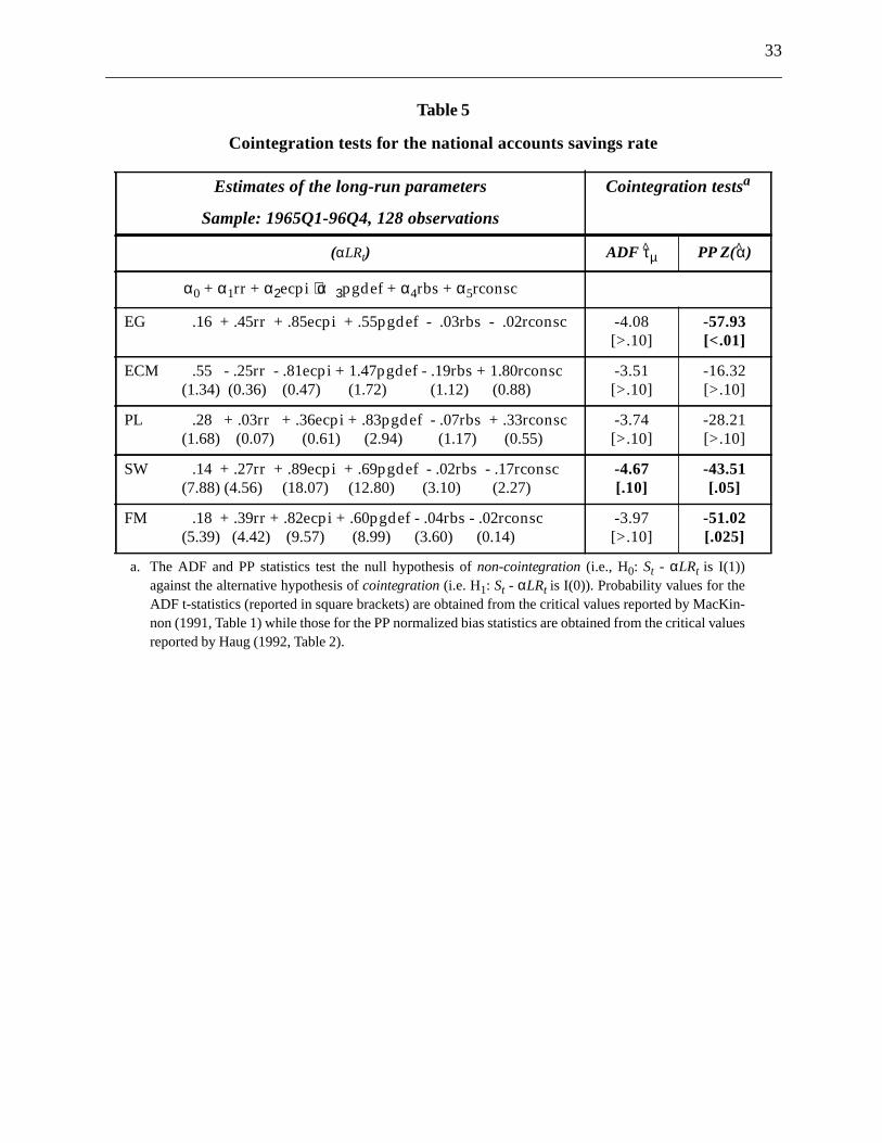
33

Table 5

Cointegration tests for the national accounts savings rate

Estimates of the long-run parameters

Sample: 1965Q1-96Q4, 128 observations

Cointegration testsa

a. The ADF and PP statistics test the null hypothesis ofnon-cointegration(i.e., H0: St - αLRt is I(1))against the alternative hypothesis ofcointegration(i.e. H1: St - αLRt is I(0)). Probability values for theADF t-statistics (reported in square brackets) are obtained from the critical values reported by MacKin-non (1991, Table 1) while those for the PP normalized bias statistics are obtained from the critical valuesreported by Haug (1992, Table 2).

(αLRt) ADF τµ PP Z(α)

α0 + α1rr + α2ecpi + α3pgdef + α4rbs + α5rconsc

EG .16 + .45rr + .85ecpi + .55pgdef - .03rbs - .02rconsc -4.08

[>.10]

-57.93[<.01]

ECM .55 - .25rr - .81ecpi + 1.47pgdef - .19rbs + 1.80rconsc

(1.34) (0.36) (0.47) (1.72) (1.12) (0.88)

-3.51

[>.10]

-16.32

[>.10]

PL .28 + .03rr + .36ecpi + .83pgdef - .07rbs + .33rconsc

(1.68) (0.07) (0.61) (2.94) (1.17) (0.55)

-3.74

[>.10]

-28.21

[>.10]

SW .14 + .27rr + .89ecpi + .69pgdef - .02rbs - .17rconsc

(7.88) (4.56) (18.07) (12.80) (3.10) (2.27)

-4.67[.10]

-43.51[.05]

FM .18 + .39rr + .82ecpi + .60pgdef - .04rbs - .02rconsc

(5.39) (4.42) (9.57) (8.99) (3.60) (0.14)

-3.97

[>.10]

-51.02[.025]

34

Table 6

Cointegration tests for the national accounts savings rate

Estimates of the long-run parameters

Sample: 1965Q1-96Q4, 128 observations

Cointegration testsa

Error-correction term ( )

a. The ADF and PP statistics test the null hypothesis of non-cointegration (i.e., H0: St - αLRt is I(1)) against thealternative hypothesis of cointegration (i.e., H1: St - αLRt is I(0)). Probability values for the ADF t-statistics(reported in square brackets) are obtained from the critical values reported by MacKinnon (1991, Table 1)while those for the PP normalized bias statistics are obtained from the critical values reported by Haug (1992,Table 2). The error-correction term is represented by the parameter and the critical values forτγ in the caseof the ECM one-step procedure are from Banerjee et al. (1993, Table 4).

(αLRt) ADF τµ PP Z(α) ECM:τγ

α0 + α1rr + α2ecpi + α3pgdef + α4rbs γ

EG .16 + .45rr + .85ecpi + .55pgdef - .03rbs -4.09

[>.10]

-58.17[<.01]

-0.21(2.25)

ECM .21 + .26rr + .77ecpi + .84pgdef - .04rbs

(2.88) (1.33) (4.41) (4.27) (2.54)

-3.76

[>.10]

-36.88[.10]

-0.25(2.42)

PL .12 + .35rr + .99ecpi + .60pgdef - .02rbs

(1.65) (1.58) (5.07) (2.57) (1.40)

-4.69[.025]

-47.15[.025]

-0.22(2.24)

SW .11 + .33rr + .96ecpi + .68pgdef - .02rbs

(4.75) (4.98) (15.00) (8.29) (3.95)

-4.74[.025]

-45.43[.025]

-0.23(2.32)

FM .15 + .48rr + .90ecpi + .58pgdef - .03rbs

(4.19) (4.90) (10.00) (8.26) (3.78)

-4.35[.10]

-58.22[<.01]

-0.23(2.35)

γ

γ

35

Table 7

Sensitivity analysis of the national accounts savings rate long-run equation estimates

Stability tests

(Sample: 1965Q1-96Q4, 128 observations)

Table 8

Sensitivity analysis of the national accounts savings rate long-run equation estimates

Alternative measure of expected inflation from Markov-switching model

(Sample: 1965Q1-96Q4, 128 observations)

Estimates of long-run parametersa

a. The estimates of the long-run parameters reported above are obtained using the Phillips-Hansen fully mod-ified estimator procedure (FM) as presented in the last row of Tables 5 and 6. The FM estimator uses resid-uals that are prewhitened with a VAR(2) to correct for serial correlation.

Stability testsb

b. The Lc, MeanF and SupF tests examine the null hypothesis of a stable long-run relationship among I(1)variables against different alternative hypotheses. A rejection of the null hypothesis provides evidence ofparameter instability. Probability values are reported in square brackets.

(αLRt) Lc MeanF SupF

.18 + .39rr + .82ecpi + .60pgdef - .04rbs - .02rconsc

(5.39) (4.42) (9.57) (8.99) (3.60) (0.14)

0.78

[.15]

11.45

[.03]

27.50

[.01]

.15 + .48rr + .90ecpi + .58pgdef - .03rbs

(4.19) (4.90) (10.00) (8.26) (3.78)

0.53

[>.20]

6.67

[.19]

19.62

[.04]

Estimates of long-run parameters Cointegration testsa

a. See notes to Table 5.

(αLRt) ADF τµ PP Z(α)

α0 + α1mrr + α2msm + α3pgdef + α4rbs

ECM .21 + .29mrr + .78msm + .80pgdef - .04rbs

(3.30) (1.43) (4.79) (4.41) (2.89)

-3.98

[>.10]

-68.35[<.01]

PL .12 + .40mrr + 1.06msm + .52pgdef - .02rbs

(1.88) (2.00) (5.96) (2.53) (1.60)

-3.71

[>.10]

-66.45[<.01]

SW .12 + .38mrr + .95msm + .66pgdef - .02rbs

(5.55) (5.73) (16.22) (7.23) (4.81)

-4.63[.05]

-73.74[<.01]

36

Table 9

Sensitivity analysis of the national accounts savings rate long-run equation estimates

2th-order dynamic specification

(Sample: 1965Q1-96Q4, 128 observations)

Estimates of the long-run parameters Cointegration testsa

a. See notes to Table 5.

(αLRt) ADF τµ PP Z(α)

α0 + α1rr + α2ecpi + α3pgdef + α4rbs

ECM .20 + .31rr + .67ecpi +.85pgdef - .04rbs

(2.02) (1.12) (2.60) (3.14) (1.71)

-4.34[.10]

-36.37[.10]

PL .16 + .39rr + .83ecpi + .67pgdef - .03rbs

(2.68) (2.12) (5.32) (3.87) (2.30)

-4.37[.10]

-51.76[<.01]

SW .14 + .36rr + .88ecpi + .67pgdef - .03rbs

(8.24) (5.82) (17.51) (8.72) (7.45)

-4.60[.05]

-50.13[<.01]

37

Table 10

Cointegration tests for the balance-sheet savings rate

Estimates of the long-run parameters

Sample: 1965Q1-96Q4, 128 observations

Cointegration testsa

a. The ADF and PP statistics test the null hypothesis ofnon-cointegration(i.e., H0:: St - αLRt is I (1))against the alternative hypothesis ofcointegration(i.e., H1: St - αLRt is I(0)). Probability values for theADF t- statistics (reported in square brackets) are obtained from the critical values reported by MacKin-non (1991, Table 1) while those for the PP normalized bias statistics are obtained from the critical valuesreported by Haug (1992, Table 2).

(αLRt) ADF τµ PP Z(α)

α0 + α1rr + α2ecpi + α3pgdef + α4rbs

EG .61 - .24rr + .52ecpi - .38pgdef - .09rbs -3.78

[>.10]

-80.70[<.01]

PL .95 - 1.48rr + .08ecpi + 1.01pgdef - .17rbs

(3.54) (2.04) (0.12) (1.42) (2.69)

-4.00

[>.10]

-60.04[<.01]

SW .68 - .86rr + .72ecpi + 0.48pgdef - .11rbs

(8.40) (3.57) (3.95) (2.29) (5.72)

-4.29[.10]

-66.21[<.01]

α0 + α1rr + α2ecpi + α3rbs

EG .68 - .46rr + .32ecpi - .10rbs -3.86[.10]

-79.51[<.01]

PL .75 - .71rr + .45ecpi - .12rbs

(3.19) (1.41) (0.86) (2.22)

-4.16[.05]

-76.65[<.01]

SW .58 - .49rr + .89ecpi - .09rbs

(8.83) (1.99) (4.21) (5.63)

-4.40[.025]

-73.32[<.01]

39

Figure 1Net savings per major sectors as a percentage of nominal GDP

Annual averages (1961–1998)

1965 1970 1975 1980 1985 1990 1995-10

-5

0

5

10

15

-10

-5

0

5

10

15

Personal

Business

Non-residents

Government

%

40

Figure 2The national accounts measure of the personal savings rate (NIEA)

(1963Q1-97Q4)

Figure 3The balance-sheet measure of the personal savings rate (NBSA)

1965 1970 1975 1980 1985 1990 1995-5

0

5

10

15

20

-5

0

5

10

15

20

savrna

%

1965 1970 1975 1980 1985 1990 19955

10

15

20

25

30

35

40

45

50

5

10

15

20

25

30

35

40

45

50

savrbs

%

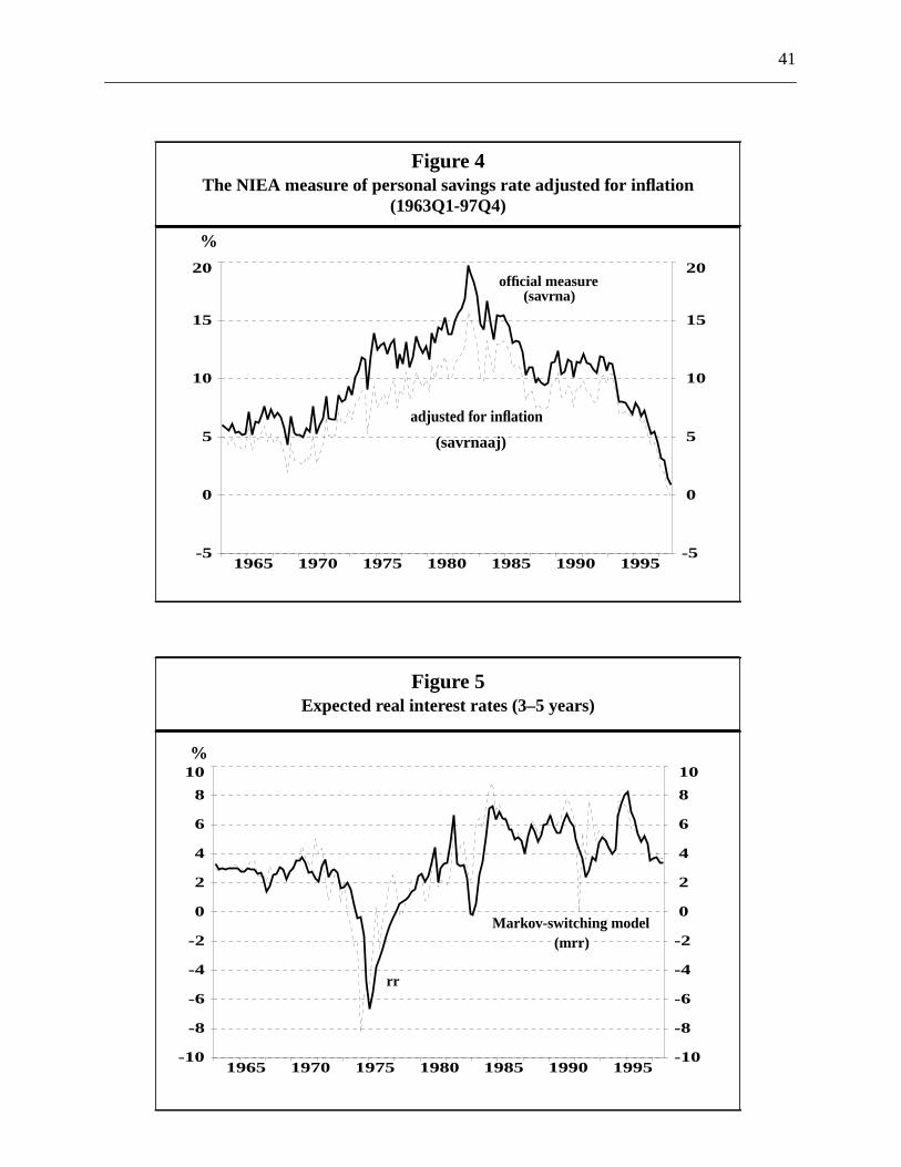
41

Figure 4The NIEA measure of personal savings rate adjusted for inflation

(1963Q1-97Q4)

Figure 5Expected real interest rates (3–5 years)

1965 1970 1975 1980 1985 1990 1995-5

0

5

10

15

20

-5

0

5

10

15

20

adjusted for inflation

official measure(savrna)

%

(savrnaaj)

1965 1970 1975 1980 1985 1990 1995-10

-8

-6

-4

-2

0

2

4

6

8

10

-10

-8

-6

-4

-2

0

2

4

6

8

10

rr

%

(mrr)Markov-switching model

42

Figure 6Expected inflation rate

(1963Q1-97Q4)

Figure 7All-government fiscal balances as a share of nominal GDP

1965 1970 1975 1980 1985 1990 19950

2

4

6

8

10

12

14

16

18

0

2

4

6

8

10

12

14

16

18

ecpi

Markov-switching model

%

(msm)

1965 1970 1975 1980 1985 1990 1995-4

-2

0

2

4

6

8

10

-4

-2

0

2

4

6

8

10

pgdef+ deficit

- surplus

%

43

Figure 8The unemployment rate

(1963Q1-97Q4)

Figure 9The ratio of balance-sheet net worth to personal disposable income

1965 1970 1975 1980 1985 1990 19952

4

6

8

10

12

14

2

4

6

8

10

12

14

rnu

%

1965 1970 1975 1980 1985 1990 19953.4

3.6

3.8

4.0

4.2

4.4

4.6

4.8

5.0

5.2

3.4

3.6

3.8

4.0

4.2

4.4

4.6

4.8

5.0

5.2

rbs

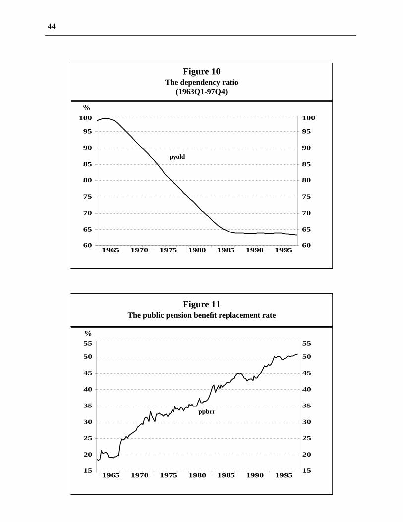
44

Figure 10The dependency ratio

(1963Q1-97Q4)

Figure 11The public pension benefit replacement rate

1965 1970 1975 1980 1985 1990 199560

65

70

75

80

85

90

95

100

60

65

70

75

80

85

90

95

100

pyold

%

1965 1970 1975 1980 1985 1990 199515

20

25

30

35

40

45

50

55

15

20

25

30

35

40

45

50

55

ppbrr

%

45

Figure 12The ratio of consumer credit to personal disposable income

(1963Q1-97Q4)

Figure 13The change in the dependency ratio

1965 1970 1975 1980 1985 1990 199514

16

18

20

22

24

26

14

16

18

20

22

24

26

rconsc

%

1965 1970 1975 1980 1985 1990 1995-0.6

-0.5

-0.4

-0.3

-0.2

-0.1

0.0

0.1

0.2

0.3

0.4

-0.6

-0.5

-0.4

-0.3

-0.2

-0.1

0.0

0.1

0.2

0.3

0.4

dpyold

%

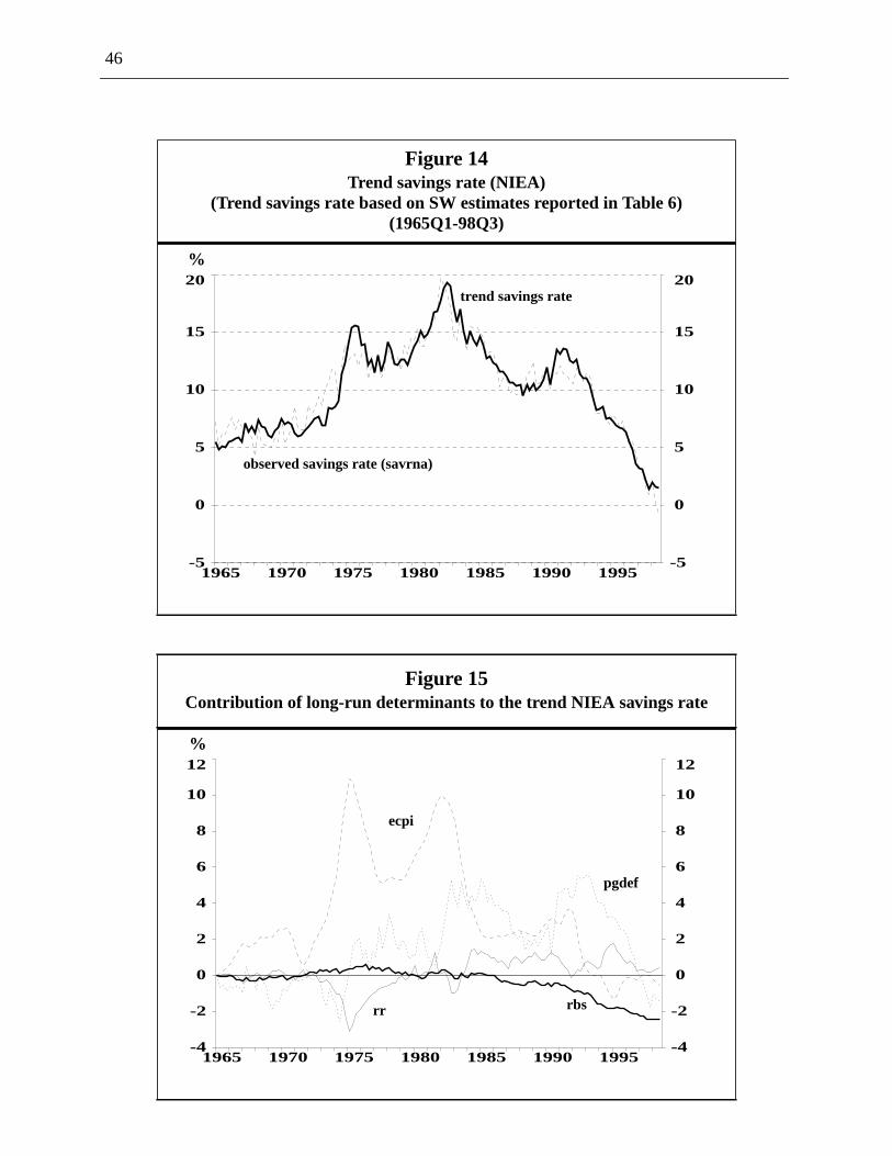
46

Figure 14Trend savings rate (NIEA)

(Trend savings rate based on SW estimates reported in Table 6)(1965Q1-98Q3)

Figure 15Contribution of long-run determinants to the trend NIEA savings rate

1965 1970 1975 1980 1985 1990 1995-5

0

5

10

15

20

-5

0

5

10

15

20trend savings rate

observed savings rate (savrna)

%

1965 1970 1975 1980 1985 1990 1995-4

-2

0

2

4

6

8

10

12

-4

-2

0

2

4

6

8

10

12

ecpi

rbsrr

pgdef

%

47

Figure 16Trend balance-sheet savings rate (NBSA)

(Trend savings rate based on SW estimates reported in Table 10)(1965Q1-97Q4)

1965 1970 1975 1980 1985 1990 19955

10

15

20

25

30

35

40

45

50

5

10

15

20

25

30

35

40

45

50

savrbs

trend savings rate

%

49

income

ome

sureowstheatrix

l CPI

el

orth

rterlyrterlyntsthe

ationnts

Appendix 1: Description of the data1

savrna = national accounts personal saving as percentage of personal disposable(D14915/100)

savrnaaj = the NIEA personal savings rate, adjusted for inflation

savrbs = balance-sheet personal saving as percentage of personal disposable incdefined as: (diff(qknetworth)*4)/(ydp+(diff(qknetworth)*4)-savp)

ydp = personal disposable income (nominal) - D14914

savp = national accounts personal saving (nominal) - D14913

qknetworth = quarterly stock of net worth. The quarterly estimates of the net worth meahave been generated by cumulating quarterly financial flows. The flestimates are from the Financial Flow Accounts (Matrix 000701) andstocks estimates are taken from the National Balance Sheet Accounts (M000751).

ecpi = expected inflation: an eight quarter moving average of year-over-year tota(B820600) with geometrically declining weights

rr = G. of C. Bond Yield Averages (3-5 years - nominal (B14010)) minus ecpi

msm = expected inflation for total CPI (B820600) using a Markov-switching mod

mrr = G. of C. Bond Yield Averages (3-5 years - nominal (B14010)) minus msm

pgdef = all-government fiscal balances as a share of nominal GDP(-1*D15075/(D14816 or D14840)). + : Deficit; - : Surplus

rbs = ratio of quarterly stock of net worth to personal disposable income: qknetw/ydp

rconsc = ratio of consumer credit to personal disposable income (ydp). The quaconsumer credit estimates have been generated by cumulating the quafinancial flows. The flows estimates are from the Financial Flow Accou(Matrix 000701: D150070) and the stocks estimates are taken fromNational Balance Sheet Accounts (Matrix 000751: D160041).

1. The mnemonics given in parentheses refer to Cansim data series. All data series include informavailable up to the beginning of December 1998 (including the Third Quarter 1998 National Accoufrom Statistics Canada, on a 1992 base year). They are available upon request.

50

ber oftics

ior tont.

08

149

21 tonsim

ears:

rnu = the percentage of the labour force that is unemployed defined as: the numunemployed/total labour force, D980745 or D980712/D980562. The StatisCanada labour force series are available beginning in 1976. The series pr1976 have been linked at the Bank of Canada by the Research Departme

ppbrr = public pension benefit replacement rate defined as:

((old_age_security + can_pension + que_pension)/pop6599)/((ydp-(old_age_security + can_pension + que_pension))/pop1564).

old_age_security = old age security fund payments, (s.a. millions): D18144

can_pension = transfer payments to persons-Canada pension plan (s.a. millions): D151

que_pension = transfer payments to persons-Quebec pension plan (s.a. millions): D15

Population estimates per age group are from the Demographic Division. Data from 191971 are from Cansim Matrix no.: 6430. Demographic Data from 1971 to 1997 are from CaMatrix no.: 6367-6379.

pop0019 = population , 0-19 years, both sexes , CANADA (thousands)

pop1564 = population , 15-64 years, both sexes , CANADA (thousands)

pop2064 = population , 20-64 years, both sexes , CANADA (thousands)

pop6599 = population , 65+ years, both sexes , CANADA (thousands)

pyold = population age 0-19 and 65+ years as a proportion of population 20-64 y(pop0019+pop6599)/pop2064.

Nominal GDP = Gross Domestic Product at market prices: D14816 or D14840

Net personal savings: D15234

Net business savings: D15235

Net government savings: D15236

Net non-residents savings: D15237

Total net savings: D15233

Total capital consumption allowances: D15238

Total gross savings: D15233+D15238

51

tional

asure

ational

e and

nsfers

centage

te has a

holds’

ore, an

aving,

ovided

f fixed

osses

urns on

This

eholds

tion,

at the

n.

s and

rather

stretch

in the

which

IEA

assets

Appendix 2: Two measures of the personal savings rate

Our empirical work uses two different measures of the personal savings rate: the conven

measure from the National Income and Expenditure Accounts (NIEA), and an alternative me

defined as the change in the net worth position of the personal sector, as measured in the N

Balance Sheet Accounts (NBSA).1

In the NIEA, personal saving is the difference between personal disposable incom

outlays. The bulk of the outlays consists of personal consumption but also includes current tra

from persons to corporations and to non-residents. The personal savings rate is then the per

of personal saving to personal disposable income. This measure of the personal savings ra

number of shortcomings (Dagenais 1992).

On theoretical grounds, personal saving can be defined to equal the change in house

wealth, or equivalently, as a broad measure of disposable income less consumption. Theref

appropriate measure of saving requires that disposable income includes all returns on prior s

and that returns be measured in real terms. Also, consumption should include the services pr

by consumer durables, rather than the gross outlay, and should reflect the depreciation o

physical assets. However, in the NIEA, returns on prior saving do not reflect capital gains or l

caused by changes in the market value of physical and financial assets. Furthermore, the ret

prior saving included in the NIEA measure of income are measured in nominal terms.

treatment does not recognize that a portion of interest and dividend income received by hous

is simply compensation for the erosion of the real value of their asset holdings owing to infla

and hence does not increase households’ real net worth. An implication of this treatment is th

conventional measure of the personal savings rate tends to rise and fall with the rate of inflatio

Also, in the NIEA, personal consumption and personal expenditure on consumer good

services are equivalent. Although expenditure on consumer durables is akin to investment

than consumption—since the associated stream of services provided by these goods may

over a long period of time—expenditure on consumer durables is classified as consumption

year in which it takes place. (This is unlike the housing services received by homeowners, for

the NIEA include an imputed rent in current expenditure.) An additional drawback of the N

estimate of consumption is that it does not take into account the depreciation of physical

owing to wear and tear.

1. See Statistics Canada (1989) for a description of the NIEA and NBSA.

52

e and

nslate

end to

iven the

rors in

worth

entional

re not

flect

ake into

change

nce, in

ctures,

ities are

, or at

e and

een

hemes

s

been

sing the

e thissectories ofness

credit,l and

ed as

A,rtains that

Also, since personal saving is obtained as the difference between current incom

current outlays, any measurement errors in the calculation of personal income or outlays tra

directly into errors in the measure of personal saving. Important data for the personal sector t

be estimated as residuals from the activities of other sectors that are easier to measure. G

relative magnitude of personal income and personal outlays, relatively small measurement er

either of these aggregates can be quite large in relation to personal saving.2

The change in the National Balance Sheet Accounts’ estimate of personal net

provides an alternative measure of saving that presents several advantages over the conv

measure. Estimates of personal net worth in the National Balance Sheet Accounts (NBSA) a

affected by the inflation premium in asset returns. Also, the NBSA estimates of net worth re

changes in asset values, include the stock of consumer durables in personal assets, and t

account the depreciation of physical assets.

Although closer to the relevant theoretical concepts, a saving measure based on the

in the NBSA estimates of personal wealth also presents a number of shortcomings. For insta

the NBSA, assets are not recorded at their market value: tangible assets (residential stru

consumer durables) are measured at replacement cost while most financial assets and liabil

recorded either at book value (i.e., acquisition cost), as in the case of government bonds

“current value,” as is the case for equity, with current value obtained as the sum of book valu

cumulated retained earnings.3 Also, household savings held in mutual funds that have not b

established solely for investing the proceeds of RRSP contributions and similar tax shelter sc

are not included in the estimate of personal net worth.4 Furthermore, as in the NIEA, the value

ascribed to most of the asset and liability items of the personal sector in the NBSA have

obtained as residuals from the activities of the other sectors. Hence, all errors made in asses

values pertaining to the other sectors affect the net worth estimates of the personal sector.5

2. In addition, the personal sector includes the activities of the unincorporated business sector, sincsector is not accounted for elsewhere in the national accounts. The unincorporated businessencompasses private non-profit institutions, trusteed pension plans, and the investment activitlife insurance companies. Clift (1988) suggests that the inclusion of the unincorporated busisector has little impact on measured personal saving.

3. The most important items in the balance sheet of the personal sector are mortgages, consumerand bank loans on the liability side, and shares, currency and deposits, bonds (mainly federaprovincial government bonds), life insurance, and pensions on the asset side.

4. Note also that contributions to public pension plans and related investment income are not counthousehold savings because households do not own these plans.

5. Human capital is omitted from the NBSA measure of personal net worth. Similarly, in the NIEspending on education, training, and health is treated entirely as consumption when in fact cetypes of health, training, and education services could be regarded as investment on the groundthey increase the expected life and productivity of a nation’s stock of human capital.

53

tion

sis.

sts of

Paper

ehold

ent and

Time

Bibliography

Akaike, H. 1969. “Statistical Predictor Identification.”Annals of the Institute of Statistical Mathematics21:203–207.

Andrews, D. W. K. and J. C. Monahan. 1992. “An Improved Heteroskedasticity and AutocorrelaConsistent Covariance Matrix Estimator.”Econometrica60: 953–966.

Aubry, J. P. and D. Fleurent. 1980.Simulation Analysis of a Model Based on the Life-Cycle HypotheTechnical Report No. 18. Ottawa: Bank of Canada.

Banerjee, A., J. J. Dolado, and R. Mestre. 1993. “On Some Simple Tests for Cointegration: the CoSimplicity.” Bank of Spain Working Paper No. 9302.

Banks, J., R. Blundell, and S. Tanner. 1998. “Is There a Retirement-Savings Puzzle?”AmericanEconomicReview88 : 769–788.

Beach, C. M., R. W. Boadway, and N. Bruce. 1988. “Taxation and Savings in Canada.” Technicalprepared for the Economic Council of Canada.

Bernheim, B. D. 1987. “Ricardian Equivalence: An Evaluation of Theory and Evidence.” InNBERMacroeconomics Annual, edited by S. Fischer. Cambridge, MA: MIT Press.

———. 1989. “A Neoclassical Perspective on Budget Deficits.”Journal of Economic Perspectives3 (2):55–72.

Bernheim, B. D., A. Shleifer, and L. H. Summers. 1985. “The Strategic Bequest Motive.”Journal of PoliticalEconomy93: 1045–1076.

Blanchard, O. J. 1985. “Debt, Deficits, and Finite Horizons.”Journal of Political Economy93:223–247.

Bosworth, B., G. Burtless, and J. Sabelhaus. 1991. “The Decline in Saving: Evidence from HousSurvey.”Brookings Papers on Economic Activity1: 183–256.

Bovenberg, A. L. and O. Evans. 1989. “National and Personal Saving in the United States: MeasuremAnalysis of Recent Trends.” IMF Working Paper/89/99.

Boyle, P. and J. Murray. 1979. “Social Security Wealth and Private Saving in Canada.”Canadian Journal ofEconomics12: 456–468.

Browning, M. and A. Lusardi. 1996. “Household Saving: Micro Theories and Micro Facts.”Journal ofEconomic Literature34: 1797–1855.

Buiter, W. H. 1988. “Death, Birth, Productivity Growth and Debt Neutrality.”Economic Journal98: 279–293.

Burbidge, J. B. and J. B. Davies. 1994. “Government incentives and houseold saving in Canada.’ InPublicPolicies and Household Saving, edited by J. M. Poterba. Chicago: University of Chicago Press.

Campbell, J. Y. and N. G. Mankiw. 1989. “Consumption, Income and Interest Rates: Reinterpreting theSeries Evidence.” NBER Working Paper No. 2924.

54

ction

No.

anada

on:

.

s

rking

nada.”

lan on

wing

Campbell, J. Y. and N. G. Mankiw. 1991. “The Response of Consumption to Income, A Cross-SeInvestigation.”European Economic Review35: 723–767.

Canada. Statistics Canada. 1989.A User Guide to the Canadian System of National Accounts. Cat. No. 13-589E (Occasional).

Carroll, C. D. 1992. “The Buffer-Stock Theory of Saving: Some Macroeconomic Evidence.”BrookingsPapers on Economic Activity2: 61–156.

———. 1997. “Buffer-Stock Saving and the Life Cycle/Permanent Income Hypothesis.”Quarterly Journalof Economics112: 1–55.

Carroll, C. D. and A. A. Samwick. 1995. “The Nature of Precautionary Wealth.” NBER Working Paper5193.

Carroll, C. and L. H. Summers. 1987. “Why Have Private Savings Rates in the United States and CDiverged?”Journal of Monetary Economics20: 249–279.

———. 1991. “Consumption Growth Parallels Income Growth: Some New Evidence.” InNational Savingand Economic Performance, edited by B. D. Bernheim and J. B. Shoven. Chicago and LondUniversity of Chicago Press.

Clift, B. 1988. “Components of Personal Saving.”Canadian Economic Observer. Ottawa: Statistics Canada

Coiteux, M. 1998. “Are Canadian Households Getting Richer by Saving Less?”École des Hautes ÉtudesCommerciales (HÉC). Mimeo. (Published later in December 1999 inCanadian Business Economic7 (4): 79–89.)

Cozier, B. and G. Tkacz. 1994. “The Term Structure and Real Activity in Canada.” Bank of Canada WoPaper No. 94-3.

Dagenais, M. G. 1992. “Measuring Personal Savings, Consumption, and Disposable Income in CaCanadian Journal of Economics25: 681–707.

Daly, M. 1983. “Some Microeconometric Evidence Concerning the Effect of the Canada Pension PPersonal Saving.”Economica50: 63–69.

Davidson, R. and J. G. MacKinnon. 1993.Estimation and Inference in Econometrics.New York: OxfordUniversity Press.

Davies, J. 1981. “Uncertain Lifetime, Consumption, and Dissaving in Retirement.”Journal of PoliticalEconomy89: 561–577.

Deaton, A. S. 1977. “Involuntary Savings Through Unanticipated Inflation.”American Economic Review67: 899–910.

De Gregorio, J. 1993. “Savings, Growth and Capital Markets Imperfections: The Case of BorroConstraints.” IMF Working Paper 93-31.

Denny, M. and S. A. Rea, Jr. 1979. “Pensions and Saving in Canada.” InSocial Security Versus PrivateSaving, Volume 1, edited by G. M. Von Furstenberg. Cambridge, MA: Ballinger.

Diamond, P. A. 1977. “A Framework for Social Security Analysis.”Journal of Public Economics8: 275–298.

55

ith a

ess.”

g.” Inton:

ation

ank of

s.” Innd

te of

RWP

tion --

Dickey, D. A. and W. A. Fuller. 1979. “Distribution of the Estimators for Autoregressive Time Series wUnit Root.”Journal of the American Statistical Association74: 427–431.

Dicks-Mireaux, L. and M. King. 1984. “Pension Wealth and Household Savings: Tests of RobustnJournal of Public Economics23: 115–139.

Engen, E. M. and W. G. Gale. 1997. “Effects of Social Security Reform on Private and National SavinSocial Security Reform, edited by S. A. Sass and R. K. Triest. Conference Series No. 41. BosFederal Reserve Bank of Boston.

Engle, R. F. and C. W. J. Granger. 1987. “Co-Integration and Error Correction: Representation, Estimand Testing.”Econometrica55: 251–276.

Evans, O. 1983. “Social Security and Household Saving in the United States: A Re-Examination.”IMF StaffPapers30: 601–618.

Feldstein, M. 1974. “Social Security, Induced Retirement, and Aggregate Capital Accumulation.”Journal ofPolitical Economy82: 905–926.

———. 1980. “International Differences in Social Security and Saving.”Journal of Public Economics14:225–244.

———. 1995. “Social Security and Saving: New Time Series Evidence.” NBER Working Paper 5054.

Fillion, J.-F. 1996. “L’endettement du Canada et ses effets sur les taux d’intérêts de long terme.” BCanada Working Paper No. 96-14.

Friedman, B. M., and M. Warshawsky. 1988. “Annuity Prices and Saving Behavior in the United StatePensions in the U.S. Economy,edited by Z. Bodie, J. B. Shoven, and D. A. Wise. Chicago: NBER aUniversity of Chicago Press.

Granger, C. W. J. and P. Newbold. 1974. “Spurious Regressions in Econometrics.”Journal of Econometrics2: 111–120.

Hansen, B. E. 1992. “Tests for Parameter Instability in Regressions with I(1) Processes.”Journal of Businessand Economic Statistics10: 321–335.

Hansen, H. and K. Juselius. 1995. “CATS in RATS: Cointegration Analysis of Time Series.” InstituEconomics, University of Copenhagen.

Haug, A. A. 1992. “Critical Values for theZα - Phillips-Ouliaris Test for Cointegration.”Oxford Bulletin ofEconomics and Statistics54: 473–480.

Hess, G. D. and B. K. Wilson. 1994. “Reinterpreting Excess Sensitivity with Precautionary Savings.”94-10, Federal Reserve Bank of Kansas City.

Jappelli, T. and M. Pagano. 1994. “Saving, Growth, and Liquidity Constraints.”Quarterly Journal ofEconomics109: 83–109.

Johansen, S. 1988. “Statistical Analysis of Cointegration Vectors.”Journal of Economic Dynamics andControl12: 231–254.

Johansen, S. and K. Juselius. 1990. “Maximum Likelihood Estimation and Inference on CointegraWith Applications to the Demand for Money.”Oxford Bulletin of Economics and Statistics52: 169–210.

56

and

nada.”

l Paper

d

ries.”look

No.

Rolen the

r the

PE/

m

ment

Kotlikoff, L. J. 1988. “Intergenerational Transfers and Savings.”Journal of Economic Perspectives2: 41–58.

Kotlikoff, L. J., J. Shoven, and A. Spivak. 1986. “The Effect of Annuity Insurance on SavingsInequality.”Journal of Labor Economics4: S183–S207.

Kremers, J., N. Ericsson, and J. Dolado. 1992. “The Power of Cointegration Tests.”Oxford Bulletin ofEconomics and Statistics54: 325–348.

Lau, H.-H. 1993. “Behaviour of the personal saving rate in Canada in recent years: A note.”Bank of CanadaReview(Spring): 57–68.

———. 1997. “Recent developments in the personal sector financial position and savings in CaResearch Department, Bank of Canada, March 31.

Mackenzie, G. A., P. Gerson, and A. Cuevas. 1997. “Pension regimes and Saving.” IMF Occasiona153.

MacKinnon, J. G. 1991. “Critical Values for Cointegration Tests.” Chapter 13 inLong-Run EconomicRelationships: Readings in Cointegration, edited by R. Engle and C. Granger. Oxford: OxforUniversity Press.

Macklem, R. T. 1994.Wealth, Disposable Income and Consumption: Some Evidence for Canada.TechnicalReport No. 71. Ottawa: Bank of Canada.

Masson, P., T. Bayoumi, and H. Samiei. 1995. “Saving Behavior in Industrial and Developing CountWorld Economic and Financial Surveys, IMF Staff Studies for the World Economic Out(September): 1-27.

Meredith, G. 1995. “Demographic Change and Household Saving in Japan.” InSaving Behavior and theAsset Price “Bubble” in Japan, edited by U. Baumgartner and G. Meredith. Occasional Paper124.

Modigliani, F. and A. Sterling. 1980. “Determinants of National Saving with Special Reference to theof Social Security - Cross Country Tests.” International Economic Association Conference oDeterminants of National Saving and Wealth, Bergamo, 9–14 June, 1980.

Montplaisir, M.-C. 1996–1997. “The maturity structure of household financial assets and liabilities.”Bank ofCanada Review(Winter): 33–46.

Ng, S. and P. Perron 1995. “Unit Root Tests in ARMA Models with Data Dependent Methods foSelection of the Truncation Lag.”Journal of the American Statistical Association90:268–281.

OECD. 1998. “The Retirement Decision in OECD Countries.” ECO/CPE/WP1(98)2 and ECO/CWP1(98)2/ANN1.

Osterwald-Lenum, M. 1992. “A Note with Quantiles of the Asymptotic Distribution of the MaximuLikelihood Cointegration Rank Test Statistics.”Oxford Bulletin of Economics and Statistics54: 461–472.

Paquet, A. 1994. “A Guide to Applied Modern Macroeconometrics.” Working Paper No. 94-05, Departof Finance, Government of Canada.

57

n with

tion.”

ction

Asset

sented

”

ground, 15

rder

Phillips, P. C. B. 1986. “Understanding Spurious Regressions in Econometrics.”Journal of Econometrics33: 311–340.

Phillips, P. C. B. and B. E. Hansen. 1990. “Statistical Inference in Instrumental Variables RegressioI(1) Processes.”Review of Economic Studies57: 99–126.

Phillips, P. C. B. and M. Loretan. 1991. “Estimating Long-run Economic Equilibria.”Review of EconomicStudies58: 407–436.

Phillips, P. C. B. and S. Ouliaris. 1990. “Asymptotic Properties of Residual Based Tests for CointegraEconometrica58: 165–193.

Phillips, P. C. B. and P. Perron. 1988. “Testing for a Unit Root in Time Series Regression.”Biometrica75:335–346.

Pitarakis, J. Y. 1993. “Cointegration Analysis in Large Systems: New Test Criteria and a Model SeleProcedure.” Department of Economics, Boston University. Mimeo.

Poterba, J. M., S. F. Venti, and D.A. Wise. 1996. “Personal Retirement Saving Programs andAccumulation: Reconciling the Evidence.” NBER Working Paper 5599.

Ragan, C. 1994. “Progressive Income Taxes and the Substitution Effect of RRSP.”Canadian Journal ofEconomics27: 43–57.

Ricketts, N. 1995. “Regime switching models of expected inflation and real interest rates.” Paper preat the 1995 Meeting of the Canadian Economic Association, Montréal, Québec. 23–39.

———. 1996. “Real short-term interest rates and expected inflation: Measurement and interpretation.Bankof Canada Review(Summer): 23–39.

Sabelhaus, J. 1997. “Public Policy and Saving in the United States and Canada.”Canadian Journal ofEconomics30: 253–275.

Salgado, R. and Y. Li. 1998. “Recent Trends in Personal Saving in Canada.” Selected Issues, backinformation to the staff report on the 1997 Article IV consultation discussions with Canada, IMFJanuary.

Sandmo, A. 1970. “The Effect of Uncertainty on Saving Decisions.”Review of Economic Studies37: 353–360.

Schwarz, G. 1978. “Estimating the Dimension of a Model.”Annals of Statistics6: 461–464.

Smith, R. S. 1990. “Factors Affecting Saving, Policy Tools, and Tax Reform: A Review.”IMF Staff Papers37: 1–70.

Stock, J. H. and M. W. Watson. 1993. “A Simple Estimator of Cointegrating Vectors in Higher OIntegrated Systems.”Econometrica61: 783–820.

Sturm, P. H. 1983. “Determinants of Saving: Theory and Evidence.”OECD Economic Studies1: 147–196.

Summers, L. and C. Carroll. 1987. “Why Is U.S. National Saving So Low?”Brookings Papers on EconomicActivity2: 607–642.

58

Issues,with

dian

Thomas, A. and C. Towe. 1996. “Recent Trends in Personal Saving in Canada.” Canada, Selectedbackground information to the staff report on the 1996 Article IV consultation discussionsCanada, IMF, 19 March.

Weil, D. N. 1994. “The Saving of the Elderly in Micro and Macro Data.”Quarterly Journal of Economics109: 55–81.

Wirjanto, T. S. 1995. “Aggregate Consumption Behaviour and Liquidity Constraints: the CanaEvidence.”Canadian Journal of Economics28: 1135–1152.

Yaari, M. E. 1965. “Uncertain Lifetime, Life Insurance, and the Theory of the Consumer.”Review ofEconomic Studies32: 137–150.

Bank of Canada Working PapersDocuments de travail de la Banque du Canada

Working papers are generally published in the language of the author, with an abstract in both official lan-guages.Les documents de travail sont publiés généralement dans la langue utilisée par les auteurs; ils sontcependant précédés d’un résumé bilingue.

20002000-2 GAUSSTM Programs for the Estimation of State-Space Models with

ARCH Errors: A User’s Guide M. Kichian

2000-1 The Employment Costs of Downward Nominal-Wage Rigidity J. Farès and S. Hogan

199999-20 The Expectations Hypothesis for the Longer End of the Term Structure:

Some Evidence for Canada R. Lange

99-19 Pricing Interest Rate Derivatives in a Non-ParametricTwo-Factor Term-Structure Model J. Knight, F. Li, and M. Yuan

99-18 Estimating One-Factor Models of Short-Term Interest Rates D. Mc Manus and D. Watt

99-17 Canada’s Exchange Rate Regime and North American Econo-mic Integration: The Role of Risk-Sharing Mechanisms Z. Antia, R. Djoudad, and P. St-Amant

99-16 Optimal Currency Areas: A Review of the Recent Literature R. Lafrance and P. St-Amant

99-15 The Information Content of Interest Rate Futures Options D. Mc Manus

99-14 The U.S. Capacity Utilization Rate: A New Estimation Approach R. Lalonde

99-13 Indicator Models of Core Inflation for Canada R. Dion

99-12 Why Canada Needs a Flexible Exchange Rate J. Murray

99-11 Liquidity of the Government of Canada Securities Market: Stylized Factsand Some Market Microstructure Comparisons to the United States T. Gravelle

99-10 Real Effects of Collapsing Exchange Rate Regimes:An Application to Mexico P. Osakwe and L. Schembri

99-9 Measuring Potential Output within a State-Space Framework M. Kichian

99-8 Monetary Rules When Economic Behaviour Changes R. Amano, D. Coletti, and T. Macklem

99-7 The Exchange Rate Regime and Canada’s Monetary Order D. Laidler

99-6 Uncovering Inflation Expectations and Risk Premiumsfrom Internationally Integrated Financial Markets B.S.C. Fung, S. Mitnick, and E. Remolona

99-5 The Quantity of Money and Monetary Policy D. Laidler

99-4 An Intraday Analysis of the Effectiveness of Foreign ExchangeIntervention N. Beattie and J-F. Fillion

99-3 Forecasting GDP Growth Using Artificial Neural Networks G. Tkacz and S. Hu

Copies and a complete list of working papers are available from:Pour obtenir des exemplaires et une liste complète des documents de travail, prière de s’adresser à:

Publications Distribution, Bank of Canada Diffusion des publications, Banque du Canada234 Wellington Street Ottawa, Ontario K1A 0G9 234, rue Wellington, Ottawa (Ontario) K1A 0G9

E-mail / Adresse électronique: publications@bank-banque-canada.caWWW: http://www.bank-banque-canada.ca/