THE IMPACT OF HURRICANES ON HOUSING PRICES: EVIDENCE FROM US COASTAL CITIES

ANTHONY MURPHY AND ERIC STROBL

RESEARCH DEPARTMENT

WORKING PAPER 1009

 

 

Federal Reserve Bank of Dallas

1

The Impact of Hurricanes on Housing Prices:

Evidence from US Coastal Cities*

Anthony Murphy

Federal Reserve Bank of Dallas

and

Eric Strobl Ecole Polytechnique

October 2010

Abstract

We investigate the effect of hurricane strikes on housing prices in US coastal cities. To this end, we construct a new index of hurricane destruction which varies over time and space. Using this index and an annual, two equation, dynamic equilibrium correction panel model with area and time fixed effects, we model the effects of hurricanes on real house prices and real incomes. In our model hurricanes have a direct effect on house prices and an indirect effect via a fall in local incomes. Our results show that the typical hurricane strike raise real house prices for a number of years, with a maximum effect of between 3 to 4% three years after occurrence. There is also a small negative effect on real incomes. These results are stable across models and sub-samples. JEL Classification: Q56, R20

Keywords: hurricanes, housing prices, US coastal cities.

*We thank our discussant Cliff Kerr and other session participants at the 2010 American Economic Association Meeting for their useful comments. The views expressed are those of the authors and not those of the Federal Reserve Bank of Dallas or the Federal Reserve System. The authors are responsible for any errors or omissions.

2

Section 1: Introduction

The general fascination with hurricanes is in large part attributable to their potentially

devastating destructiveness. For instance, Hurricane Andrew in August 1992 demolished

large parts of the southeastern part of Florida, where the total cost has been estimated to have

been at least US$20 billion dollars. An important part of the damages due to hurricanes is of

course due to destruction of residential property. In the case of Hurricane Andrew, for

example, it is believed that around 25,000 homes were completely destroyed while another

100,000 were damaged (Fronstin and Holtmann, 1994). More recently, Ewing et al. (2007, p.

315) point out that Hurricane Katrina in August 2005:

“…wreaked havoc on the United States. The total impact of this killer storm in all of

its human and environmental dimensions will not be determined for several years.

Estimates of the monetary impact indicate that Katrina was the costliest storm in U.S.

history. More than a million Gulf Coast residents were displaced by the storm.”

Ewing et al. (2009) cite insured losses of $81 billion and a death toll (including indirect

deaths) of over 1,800 lives.

A large exogenous shock to housing supply such as a hurricane may, of course, have

considerable implications for the real estate market, although the a priori net effect is not

clear.1 On the one hand, the shortage in supply is likely to cause an increase in prices in the

short run. In other words, markets surge from a housing shortage immediately following a

storm and then correct in the medium and long term as supply gradually returns to prior

levels. At the same time, however, hurricanes may cause enough disruption to local

economic activity so as to negatively affect income and consequently the demand for

housing, at least in the short run.2 Moreover, if in response to the hurricane strike, current or

potential homeowners update their subjective probability of a hurricane strike occurring, this 1 Belasen and Polachek (2008) similarly note that the effect of hurricanes on wages and employment in local

labour markets is not obvious, a priori. 2 Strobl (2009) found that an average destructive hurricane caused per capita economic growth rates in US

coastal counties to fall by 0.8 percentage points, but then partially recover by 0.2 percentage points. While the

pattern is qualitatively similar at the state level, the net effect over the long term is negligible.

3

may reduce the attractiveness of hurricane-prone areas and reduce housing demand even in

the long-run.

While there are a now a handful of studies of the impact of hurricane strikes on

housing prices, the empirical evidence is rather inconclusive. For instance, Bin and Polasky

(2004) study residential property values in Pitt County, North Carolina between 1992 and

2002 using a hedonic price model and find that the flooding due to Hurricane Floyd in 1999

reduced the market value of houses inside floodplain areas. On the other hand, focusing on

much larger areas, Graham and Hall (2001), Beracha and Prati (2008), and Speyrer and

Ragas (1991) find no discernable effect of hurricane strikes on house prices. In contrast,

Aqeel (2009) using difference-in-difference pooled OLS regressions and quarterly data for 75

MSAs from 2000 to 2008, finds that that Hurricane Katrina caused house prices in directly

affected areas to rise by about 7 per cent, with a smaller increase in nearby areas.

Taking a slightly different approach, Hallstrom and Smith (2005) focus on the impact

of hurricanes on house prices in nearby but unaffected counties and discover that house prices

dip by as much as 19 per cent in a hedonic pricing model, suggesting that there is a proximity

effect due to the updating of subjective beliefs on the probability of occurrence. Carbone,

Hallstrom and Smith (2006) obtain similar results. Using a difference in difference model and

repeat home sales data, they find that Hurricane Andrew in 1992 significantly reduced the

increase in home prices from 1993 to 2000 in areas of two coastal counties in Florida which

are prone to storm surge flooding, consistent with increased perception of risk on the part of

the public.3

In this paper, we re-examine this effect of hurricanes on house prices in US coastal

cities. We make three contributions to the literature. Firstly, we use a more general house

price model than other studies. Our model includes both short run house price and income

dynamics as well as long run equilibrium correction terms. These short and long run terms

are the so-called “bubble builder” and “bubble burster” effects found in almost all

3 The two counties are Dade County, where the majority of the damage caused by Hurricane Andrew occurred,

and Lee County, which was largely unaffected.

4

econometric house price models (e.g. Abraham and Hendershott, 1996). In addition, we

model the effect of hurricane strikes on both house prices and incomes. In our model

hurricanes have a direct effect on house prices and an indirect effect via a fall in local

incomes.

Secondly, previous studies have modeled hurricane strikes solely in terms of whether

or not they affected a local area. However, hurricanes are large spatial phenomena and their

destructive effect varies over time and across space. For example, the same hurricane will

have different destructive effects in different areas depending on where these areas are

located relative to the ‘eye’ of the hurricane, the hurricane’s maximum wind speed at the time

and the level of local property exposed. In this paper we capture these effects using a

hurricane destruction index. The index is based on a monetary loss equation, local wind speed

estimates derived from a physical wind field model as well as local exposure characteristics.

This hurricane destruction index dominates a simple hurricane incidence indicator.

Thirdly, our annual, panel dataset of coastal areas (CBSA’s) covers a longer time

period, more areas and includes more hurricanes strikes than many other studies. Using this

dataset and our index of hurricane destructiveness, we are able to estimate and test quite

general dynamic models. Our basic model is a two equation, dynamic equilibrium correction

panel model for house prices and incomes with area and time fixed effects. Our results show

that the typical hurricane strike raises real house prices for a number of years, with a

maximum effect of between 3 to 4% three years after occurrence. There is also a small

negative effect on real incomes. These results are stable across models and sub-samples.

The remainder of the paper is as follows. In the next section we provide a brief

description of hurricanes and their destructive power. Section 3 describes the construction of

our hurricane destruction proxy. In Section 4 we outline the data sources used in the

empirical analysis. Our econometric specification and subsequent results are contained in the

Section 5. Finally we conclude in Section 6.

5

2. Some Basic Facts about Hurricanes and their Destructive Power

A tropical cyclone is a meteorological term for a storm system, characterized by a low

pressure system center and thunderstorms that produce strong winds and flooding rain, which

generally first forms, and hence its name, in tropical regions of the globe.4 Depending on

their location and strength, tropical cyclones are referred to by various other names, such as

hurricane, typhoon, tropical storm, cyclonic storm, and tropical depression. Tropical storms

in the North Atlantic Basin, as we study here, are termed hurricanes if they are of sufficient

strength.5 Their season can start as early as the end of May and last until the end of

November, although it generally takes place between July and October.

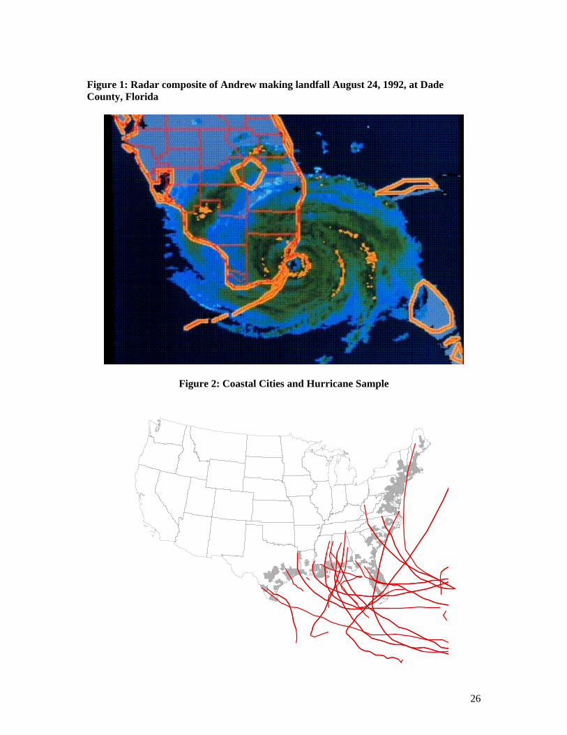
--- Figure 1 About Here ---

We depict a radar composite picture of Hurricane Andrew, which made landfall in

Florida on August 24 in 1992, as a typical example of a hurricane in Figure 1. In terms of its

structure, a hurricane will generally harbor an area of sinking air at the center of circulation,

known as the ‘eye, where weather in the eye is normally calm and free of clouds.6 Outside of

the eye curved bands of clouds and thunderstorms move away from the eye wall in a spiral

fashion, where these bands are capable of producing heavy bursts of rain, wind, and

tornadoes. One may want to note that a hurricane can affect a large area surrounding its eye

and that its structure is not symmetric. As a matter of fact, hurricane strength tropical

cyclones are on average about 500 km wide, although their size can vary considerably.

Physical damage due to hurricanes typically takes a number of forms. Firstly, the

strong winds associated with the storm may cause considerable structural damage to

buildings as well as crops. Secondly, the high winds pushing on the ocean’s surface can

4 The term "cyclone" derives from the cyclonic nature of such storms, with counterclockwise rotation in the

Northern Hemisphere and clockwise rotation in the Southern Hemisphere. 5 In order to be considered a tropical storm, the storm must have maximum wind speed of at least 55 km/hr. To

be upgraded to a hurricane these speeds must reach at least 119 km/hr. 6 National Weather Service (October 19, 2005). Tropical Cyclone Structure. JetStream - An Online School for

Weather. National Oceanic & Atmospheric Administration.

6

cause the water near the coast to pile up higher than the ordinary sea level, and this effect

combined with the low pressure at the center of the weather system and the bathymetry of the

body of water results in storm surges. Generally these surges are the most damaging aspect

of hurricanes. In particular, storm surges can cause severe property damage, as well as

destruction and salt contamination of agricultural areas.7 Such flooding may extend up to

40km or more from the coast for maximum strength storms. Finally, there is generally strong

rainfall associated with a hurricane, which can also result in extensive flooding and, in sloped

areas, landslides. One may want to note that while the latter two effects are not directly

related to wind, the extent of damage to these is highly correlated with the wind speed of a

hurricane.

3. A Hurricane Destruction Proxy

Ewing et al. (2005) used a simply incidence dummy to investigate the impact of

hurricanes on local housing prices. However, the extent of their destruction is unlikely to be

uniform across localities, but will depend on the position relative to the eye, the maximum

wind speed, direction of movement, and local characteristics, amongst other things.8 In

order to take account of the complex nature of hurricanes we thus here, as in Strobl (2009),

avail of a proxy of local wind speed experienced that is derived from a model of the spatial

structure and movement of hurricanes, and hence of wind speeds experienced directly along

the track as well as locations around it. We then translate these local wind speeds into a

proxy of local destruction. More precisely, Emanuel (2005) noted that both the monetary

losses in hurricanes as well as the power dissipation of these storms are related to their

maximum observed wind speed. Consequently, he proposed an index of hurricane damages

based on a simplified version of a power dissipation equation:

(1) 0

PDI V dt

7 Yang (2007). 8 In the case of tornados, De Silva et al. (2008) highlight the spatial dependence in housing losses due to

tornadoes.

7

where V is the maximum sustained wind speed, is the lifetime of the storm as accumulated

over time intervals t, and λ is a parameter that relates local wind speed to the local level of

damage.

We modify this index to obtain a proxy of damages due to hurricanes at the city level

using census tract data. Let i and j denote city i and census track 1 ij N respectively.

More precisely, the total destruction due to the 1 itr K storms that affected city i at time t

is defined as:

(2) 1 1

i iN K

i t i j t i j r tj r

HURR w V

where i j r tV is an estimate of the wind speed due to storm r observed in census tract j of city i

at time t. The 'si j tw are weights assigned according to characteristics of the affected census

tracks. They capture geographical differences within areas, in terms of the potential exposure

if a hurricane were to strike. Given data for V and w and a value for λ, equation (2) provides

us with a local level proxy of hurricane damages that enables us to quantify the impact of

hurricane strikes on local housing prices. In the next section we discuss the main data sources

that we used to construct our hurricane destructiveness index.

3. Data

3.1 Geographic Area of Study

Only a small proportion of the total geographic land mass of the US, namely areas

relatively close to the coast, is normally affected by hurricanes since hurricanes quickly lose

speed once they make a landfall. Moreover, as noted earlier, most hurricane damage is

caused by storm surges in coastal areas. We thus specifically focus our analysis on US

coastal areas in the North Atlantic Basin Region. In terms of the level of spatial unit of our

analysis, we are restricted by the spatial level of aggregation of the home price data,

described in greater detail below. The most disaggregated home price data are available at the

core based statistical area (CBSA) level. CBSAs consists of (i) metropolitan statistical areas,

which have at least one urbanized area of 50,000 or more population and an adjacent territory

8

that has a high degree of social and economic integration with the core in terms of

commuting ties, and (ii) micropolitan statistical areas which contain an urban core of between

10,000 and 50,000 individuals. We identified ‘coastal’ CBSA’s using the list of coastal

counties generated by the Strategic Environmental Assessments Division of the National

Oceanic and Atmospheric Administration (NOAA). Accordingly, coastal counties are

defined as those which have at least 15 per cent of their land in the coastal watershed9 or that

comprise at least 15 per cent of a coastal cataloging unit. If a CBSA intersects at least one

coastal county, we classify it as a coastal CBSA.

3.2 House Prices

Our measure of house prices within CBSAs is the Office of Federal Housing

Enterprise Oversight’s (OFHEO) quarterly housing price index (HPI).10 The HPI is a

measure of the movement of single-family house prices at the CBSA level. It is a weighted

repeat-sales index, derived from the average price changes in repeat sales or refinancing of

the same properties. As such, it is the most geographically comprehensive house price

indicator for the US.

3.3 Personal Income

We use the Bureau of Economic Analysis’ (BEA) estimates of per capita, local

personal income. Personal income in the BEA data is defined as the income received by all

persons from all sources, and constitutes the sum of net earnings by place of residence, rental

income of persons, personal dividend income, personal interest income, and personal current

transfer receipts as taken from IRS tax returns. We convert these nominal values to constant

2005 dollars using the US consumer price index. Finally, we also use the BEA’s estimate of

US national level per capita personal income, in constant 2005 dollars.

9 A coastal watershed is composed of all lands within Esturaine Drainage Areas (EDA) or Coastal Drainage

Areas (CDA) in the NOAA’s Coastal Assessment Framework. 10 The house price indices are now produced by the Federal Housing Finance Agency (FHFA).

9

The BEA discusses how natural disasters are likely to be accounted for in their

personal income estimates. In particular they argue that natural disasters will generally have

two major effects on the data. Firstly, there will be destruction of property, where property

losses net of the associated insurance claims will be incorporated as one-time effects. In this

regard, damage to property of household enterprises will reduce proprietors’ income and

rental income by the amount of uninsured losses, measured by consumption of fixed capital

less of business transfers. Damage to consumer goods, on the other hand, will affect personal

current transfer receipts net of the amount of insured losses of these goods. The second effect

of natural disasters is likely to be a disruption of the flow of income in the economy as

normal economic activity is interrupted. This will generally be embedded within the data on

which the personal income estimates are based. For example, many industries in the directly

affected area will experience a reduction in earnings as production is interrupted, while for

others there may be an increase.

3.4.1 Population weights

We use local population shares as a proxy for the relative local exposure to

hurricanes. More specifically, our census tract level population shares (i.e. the w’s in equation

(2) above) are from the decennial population censuses in 1970, 1980, 1990 and 2000, linearly

interpolated to obtain annual values for intervening years.

3.4.2 Hurricane Wind Speed

Since historical data on hurricanes normally only provide wind speeds at locations

over which the eye of the hurricane passes, one needs to estimate wind speeds for areas

surrounding the eye. Russel (1968) initiated the use of Monte Carlo simulation methods to

estimate local hurricane wind speeds and a large number of studies since then have used this

approach.11 The basic methodology in all of these studies has been to take site specific

statistics of key hurricane parameters (including the radius to maximum wind speed, heading,

translation speed, and the coast crossing position or distance to closest approach);

11 See, for instance, Batts et al. (1980) and Vickery and Twisdale (1995).

10

incorporate the sample path data into a mathematical model of hurricane wind speeds along

these paths; select random draws from the historical data; simulate the model and record the

average simulated wind speeds in areas around the eye of the hurricanes.

Here we use wind speed data generated from a new wind field model that is arguably

superior to previous methods.12 This model now provides the underlying data for hurricane

loss modeling in the well known HAZUS software.13 In this model, the full track of a

hurricane is modeled, beginning with its initiation over the ocean and ending with its final

dissipation. In essence, the model has two main components: (a) a mean flow wind model

that describes upper level winds, and, (b) a boundary layer model that allows one to estimate

wind speeds at the surface of the earth over a set of rectangular nested grids, given the

estimated upper level wind speeds.

The mean flow model underlying the HAZUS data is that developed by Vickery et al.

(2000). The model solves the full nonlinear equations of motion of a translating hurricane

and then parameterizes them for use in simulations. Compared to previous approaches, this

allows for a more accurate characterization of asymmetries in fast-moving hurricanes. The

boundary layer model of Vickery et al. (2008) is based on a combination of velocity profiles

computed using dropsond data and a linear hurricane boundary layer model. It produced

better estimates of the effect of the sea-land interface in reducing wind speeds and a more

realistic representation of the wind speeds near the surface. Extensive verification, via

comparisons of simulated and actual hurricane wind speeds, showed that this new wind speed

model provides a good representation of hurricane wind fields (FEMA, 2007). In the most

recent release of HAZUS (version MR3), the model was implemented at the census tract

level to generate maximum hurricane wind speeds per tract (if these were at least 50 miles per

hour). The model uses historical hurricane track data for all tropical storms between 1900 and

12 See FEMA (2007). 13 HAZUS is a GIS-based natural hazard loss estimation software package developed and freely distributed by

FEMA.

11

2005 that were at least SS category 3 at the time of US landfall, as recorded in the HURDAT

database.14

3.4.3 Estimation of λ

An important input variable in equation (2) is λ, the parameter that links wind speed to

its level of destruction, as derived from equation (1). In this regard Emanuel (2005) noted

that monetary damage figures of hurricanes tended to increase in the cubic power of the

maximum observed wind speed. This suggests that λ should be approximately equal to 3.

However, it should be noted that his proposed ‘cubic’ relationship between monetary

damages and wind speed is based only on a few rudimentary calculations by Southern (1979)

for Australia.

In contrast, Nordhaus (2006) conducts a more comprehensive statistical analysis and

shows that data for the US suggest that the relationship between wind speed and damages is

closer to the 8th power. More specifically, he takes data on total costs and maximum wind

speeds for a set of 20th century hurricanes. He then regresses the log of the cost per hurricane,

normalized by US GDP, on the logged maximum wind speed and finds a coefficient of

around eight. However, total US GDP is unlikely to be a good normalization for costs, since

hurricanes typically affect areas close to the coast, which constitute only a small proportion

of the US. Moreover, the relative local wealth that was affected is likely to have changed

substantially over the period, as coastal communities have grown in size and income.15

Given that many of the hurricanes in the latter half of the 20th century were particularly

strong, neglecting these features is likely to bias his estimate of λ upward. For example, if

you regress the log of the normalized cost values in Pielke et al. (2008) - who use real

hurricane damages normalized with regard to the population and wealth of the affected

counties only - on the log of the maximum observed hurricanes wind speeds in Nordhaus

14 The HURDAT database consists of six-hourly positions and corresponding intensity estimates in terms of

maximum wind speed of tropical cyclones in the North Atlantic Basin over the period 1851-2006 and is the

most complete and reliable source of North Atlantic hurricanes. 15 See Rappaport and Sachs (2003).

12

(2006), the estimated coefficient implies that costs rise to the 3.8th and not to the 8th power of

wind speed.

Given the arguable shortcomings of both Emmanuel’s (2005) and Nordhaus’ (2006)

estimates, we use the detailed information in the HAZUS dataset, which lists wind speeds at

the census tract level by affected counties, to generate a more accurate estimate of λ. We

estimate a log-linear equation relating damages to maximum wind speed:

(3) 1

ln lnr tN

r t r t r j t j r t r tj

DAMAGES N w V

where the subscripts j, r and t refer census tract j, hurricane r and time t respectively.

r tDAMAGES is the total monetary hurricane damage, r tN is the number of census tracts

affected, j r tV is the local wind speed estimate, r j tw is the share of total affected population

that is resident in affected county j and r t is a random error term. In estimating (3), the

parameter of interest is . Our hurricane damage figures are from Landsea and Pielke

(2008). Information on which census tracts were affected, as well as the corresponding wind

speed estimates, are from the HAZUS dataset. The local population shares of the affected

census tracts were calculated using our interpolated census data.

For the 1970 to 2005 period, estimating (3) produced a statistically significant

estimate of 3.35 for λ. This is much lower than the value obtained by Nordhaus (2006). We

investigated the possibility that our lower estimated is due to our shorter time span by re-

estimating (3) over the period 1900 to 2005. Given the sparse information on population size

at the census tract level prior to 1960, this limited us to estimating a county level version of

equation (3), which produced a marginally higher estimate of of 3.52, much smaller than

Nordhaus’ (2006) estimate of 8 or so. Since our estimates of λ are close to the value of 3

proposed by Emmanuel (2005), we set λ equal to 3.

Using a value of λ greater than unity implies that local damages increase more than

proportionally with the wind speed. For instance, for λ=3, if there are two regions with a

single inhabitant, then the one which is exposed to winds of 240 km/hr (level 4 on the SS

13

scale) is assumed to experience almost 14 times as much damage as the one that was

subjected to winds of only 120 km/hr (level 1 on the SS scale).

3.5 Sample

The limited OFHEO data on local area house prices means that our econometric

analysis is limited to a sub-sample of all coastal CBSAs. More specifically, we have annual

data from 1975 to 2005 for 99 CBSAs, spread over 19 coastal states, for the majority of the

variables listed above. We depict these in grey in Figure 2.

--- Figure 2 About Here ---

We have local wind field (speed) estimates for the 19 hurricanes in the HURDAT

database that made the HAZUS cut-off criteria, cited above, in the years from 1975 to 2005.16

We depict the tracks of these 19 hurricanes in Figure 2. Two points are noteworthy. Firstly,

various counties along the whole coastline were affected, especially in Florida, Alabama,

Mississippi, Louisiana, and Texas. Secondly, most hurricanes lose wind speeds fairly quickly,

and are not considered hurricanes or even tropical storms once they leave the coastal area.

3.6 The Hurricane Destruction Proxy

To demonstrate the role of the individual wind speed V and population sharea

components in our hurricane damage proxy, HURR, we consider the example of Hurricane

Andrew, shown in Figure 1. It first made landfall in Miami-Dade County in Florida on the

24th of August 1992 and then crossed into southwest Louisiana. Hurricane Andrew is

considered to be the second-most-destructive hurricane in U.S. history17, and the last of three

Category 5 hurricanes that made U.S. landfall during the 20th century. Wind speeds during

landfall reached over 115 miles per hour and storm surges as high as 5.2 meters were

16 These are Eloise [1975], Frederic [1979], Allen [1980], Alicia [1983], Elena [1985], Gloria [1985], Hugo

[1989], Andrew [1992], Opal [1995], Fran [1996], Bret [1999], Charley [2004], Frances [2004], Jeanne [2004],

Ivan [2004], Dennis [2005], Wilma [2005], Katrina [2005], and Rita [2005]. 17 It was the most destructive hurricane until the arrival of Katrina in 2005.

14

recorded in Southern Florida. In terms of damage, Andrew caused around $26.5 billion

worth ($38.1 billion in 2006 US dollars), with most of that damage cost in south Florida.

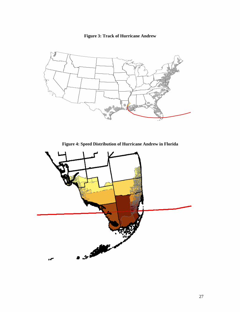
--- Figures 3 and 4 About Here ---

Hurricane Andrew’s complete track as taken from HURDAT is shown in Figure 3,

where again the red portion of the line indicates when the storm was of hurricane intensity.

As can be seen, Andrew maintained hurricane strengths even as it made a second landfall in

Louisiana, but then was reclassified as a tropical storm once it left the state. The wind speeds

generated from the HAZUS wind field model for Florida for the CBSAs in our sample along

with the actual hurricane tract (the dotted purple line) are shown in Figure 4, where darker

shading indicates stronger wind speeds. These correspond fairly well to what one would

expect for Florida from the radar composite image of the hurricane given in Figure 1. The

highest wind speeds were experienced along the track of the hurricane18, but even CBSAs

over 180km away from the actual track of the hurricane eye were subject to potential wind

damage.19

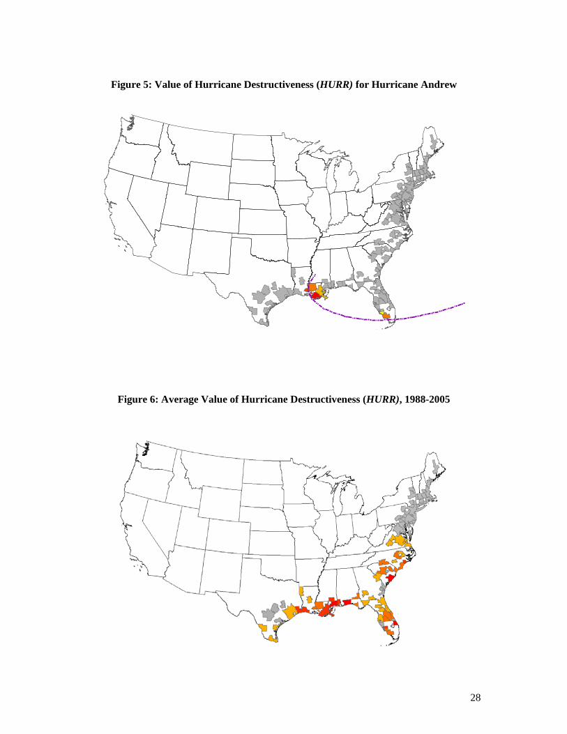
--- Figures 5 and 6 About Here ---

As an example of the impact of single hurricane on these, we graph our measure of

hurricane destructiveness, HURR, in Figure 5, where darker shading indicates higher values.

While most of the damage is found along the hurricane’s path, it is obvious that other

counties, both neighboring and further away, were also affected. In Florida, almost all of the

southern tip was affected, while in Louisiana large parts of the state was subject to damaging

wind speeds. In addition, a small part of Mississippi was affected when Andrew first entered

the state. Finally, we show the mean value of HURR for all CBSAs in our sample over our

sample period 1988 to 2005 in Figure 6. Accordingly, almost all counties were affected at

least once since the beginning of our sample period. Most destruction was, unsurprisingly

given Figure 6, suffered in Florida, Alabama, Mississippi, Louisiana, and Texas.

18 The highest wind speed, of approximately 157 miles per hour, was calculated to be in Dade County. 19 For example, census tracts within Broward County at the time of landfall experienced wind speeds of up to 92

miles per hour.

15

4. Econometric Model and Estimation Results

Our basic model is a two equation, dynamic equilibrium correction model for log real

house prices, ln ithp , and log real per capita personal disposable income ln ity , where the

subscripts i and t refer to CBSA i and year t respectively. Both variables are (1)I , i.e. have

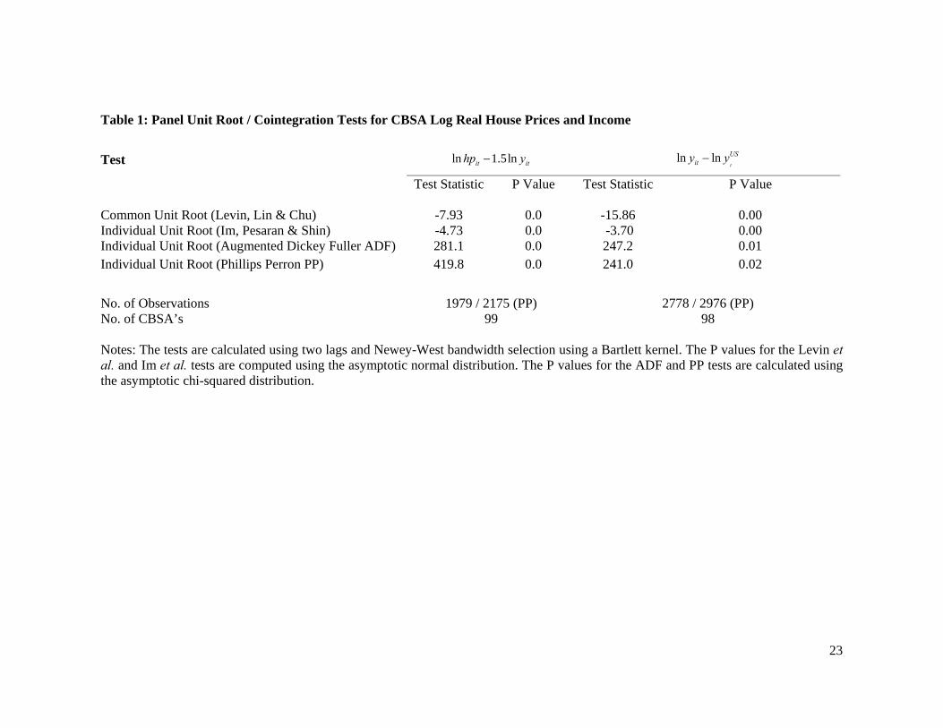
a unit root. However the panel unit root / cointegration tests in Table 1 show that, at the

CBSA level, (i) log real house prices and real income, ln ithp and ln ity , are cointegrated

with a long run elasticity of house prices w.r.t income of 1.5, and (ii) log real income at the

CBSA and national level, ln ity and ln USty , are also cointegrated with a unit coefficient.

The long run cointegrating coefficients of 1.5 and 1 were specified a priori, but these

restrictions are easily “accepted” by the data and in line with the consensus view in the

literature.20

--- Table 1 About Here ---

Inter alia, the two equation system allows hurricanes to affect both house prices and

incomes, and in turn, incomes to affect house prices. Following Abraham and Hendershott

(1996), our house price equation has both “bubble builder” (lagged house price

appreciation) and “bubble burster” (equilibrium correction) terms. The parsimonious

version of the two equation model is:

(4)

1

1 1 11 12 1 13 1

4 31 1 1 1 10

2 2 21 1 22 1

4 32 1 2 20

ln ln ln ln

ln 1.5ln

ln ln ln

ln lnt

it i t it it it

it it s t s its

it i t it it

USit s t s its

hp y hp y

hp y wspeed u

y hp y

y y wspeed u

20 Our finding that log real house prices and incomes are cointegrated at the CBSA level is consistent with the

findings of Malpezzi (1999), but at odds with those of Gallin (2006). Ideally, one would like to estimate a more

general model of long run house prices, possibly along the lines of Capozza et al. (2004).

16

where ithp = CBSA real house price, ity = CBSA real per capita personal income, USty =

US real per capita personal income, 3wspeed = weighted hurricane wind speed cubed (i.e.

HURR) and the 'su are white noise random error terms. The model has a two way (CBSA

and year) fixed effects structure represented by the parameters. The i CBSA fixed

effects pick up area specific effects, whilst the t year dummies pick up any common time

varying factors, such as changes in US personal incomes and changes in interest rates.

The terms in equation (4) capture the short run dynamics. We started with a

general, unrestricted model with four lags in ln ithp and ln ity . We then eliminated

insignificant lags to obtain the parsimonious version of the model set out above. The

equilibrium correction / long run cointegration terms are the terms with the coefficients.

Finally, current and four, unrestricted lags of weighted hurricane wind speed cubed

( 3wspeed ) are included in both equations to pick up the current and lagged effects of

hurricanes on real house prices and real incomes.

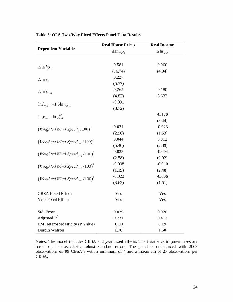
--- Table 2 About Here ---

The model was estimated in TSP (Hall and Cummins, 2005) using the least squares

dummy variables method for the year effects, which is equivalent to the panel fixed effects

method. The results are set out in Table 2. The t statistics in parentheses are based on

heteroscedastic robust standard errors. The lagged ln ithp and ln ity variables are

correctly signed and highly significant, both from an economic and statistical point of view.

Significant short run house price and income dynamics are a common feature of most

estimated house price models. The two equilibrium correction terms, 1 1ln 1.5lnit ithp y

and 11ln ln

it

USity y

, are also highly significant, although the estimated speeds of adjustment

of real house prices and real incomes to their long equilibria are relatively slow at 0.09 and

0.17 respectively.

The majority of the estimated coefficients on the weighted hurricane wind speed

cubed variables are statistically significant. In the short run, the estimated wind speed

17

coefficients in the house price equation are initially positive (lags 0 to 2) and then turn

negative (lags 3 and 4), suggesting that hurricanes raise house prices for a number of years.

--- Figure 7 About Here ---

In order to get a better feel for the results, Figure 7 show the simulated the effect of a

typical hurricane on real house prices and real incomes. The figure shows the simulated

deviations of real house prices and real per capita personal income from their baseline paths

when an average wind speed hurricane occurs at time 0. The simulation results are based on

OLS two way fixed effect estimation results set out in Table 2.

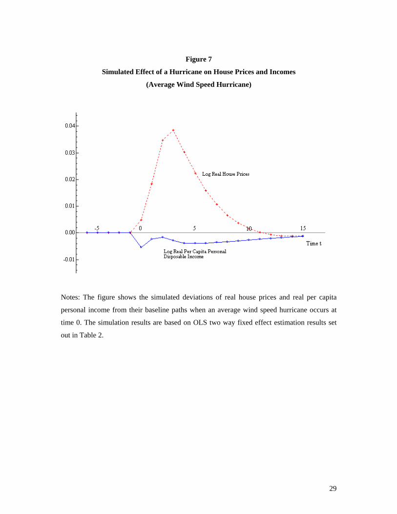
Figure 7 suggests that a typical hurricane raise real house prices in the CBSA for quite

a few years.21 It also has a small negative, albeit rather persistent, effect on real incomes.

The maximum effect on house prices shows up two to three years after the hurricane occurs,

when real house prices are about 4% higher than they would otherwise be. The economic

rationale for these results is that, in the short to medium run, most hurricanes reduce the

effective housing stock (or housing services produced by the housing stock) proportionately

more than they reduce the population living in the area, which drive up the real price of

houses (e.g. Vigdor, 2008). However, our findings are at odds with the recent findings of

Ewing et al. (2007) who, inter alia, model the change in nominal house prices in three

hurricane prone areas without including any equilibrium correction terms in their model to

tie down the long run equilibrium.22

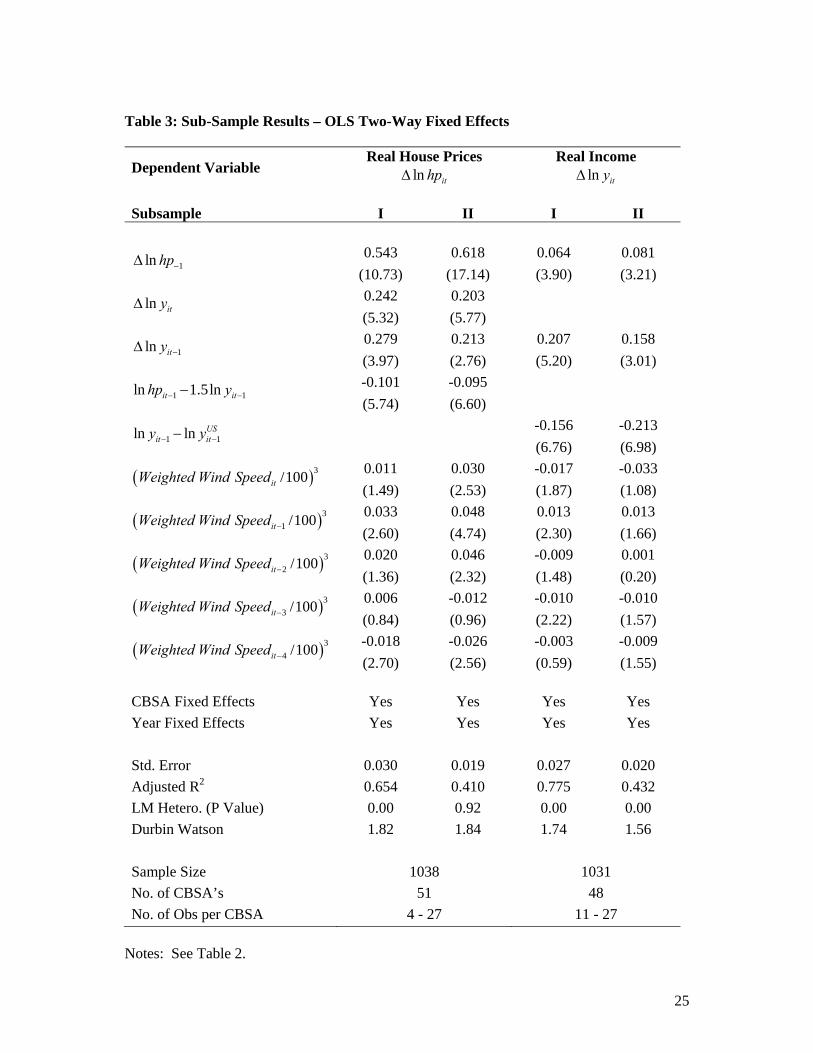
--- Table 3 About Here ---

21 Ceteris paribus, the long run level of real house prices in a CBSA is likely to be negatively affected by the

incidence of hurricanes. However, we cannot identify this effect in our model since the CBSA fixed effects

capture all CBSA time invariant, specific effects. 22 Ewing et al. (2007) model the quarterly change (log first differences) in nominal house prices in Corpus

Christ, TX, Miamai FL and Wilmington TC. Their explanatory variables are the lagged change in nominal

house prices, the current changes in state and national nominal house prices, the current change in nominal state

personal income and hurricane specific dummies as explanatory variables. Apart from the use of nominal

variables and the absence of equilibrium correction terms, endogeneity bias is likely to be an issue.

18

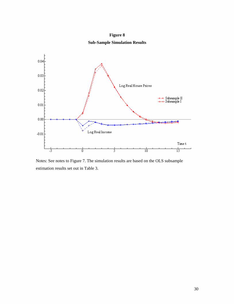
In order to check the robustness of our results, we split the sample into two arbitrary

subsamples based on CBSA number and compared the estimates (Table 3) and simulated

effects of a hurricane on real house prices and incomes (Figure 8). The results are reassuring

– the estimation results are fairly similar and the simulated effects of a hurricane are almost

identical in the two subsamples. In our model, ln ithp depends on current ln ity , inter alia,

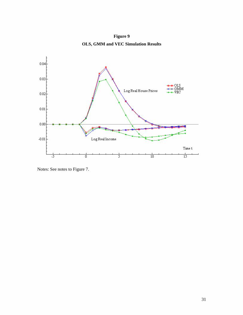
so endogeneity bias may be an issue. As a check, we estimated our model using GMM and

obtained very similar estimates of the effects of a hurricane (Figure 9).

--- Figures 8 and 9 About Here ---

Finally, we estimated a general, unrestricted vector equilibrium correction (VEC)

model i.e. a vector autoregression (VAR) with equilibrium correction terms. The VEC model

is:

(5)

1

4 4

1 1 11 121 1

4 311 1 1 12 1 1 10

4 4

2 2 21 221 1

21 1 1 22

ln ln ln

ln 1.5ln ln ln

ln ln ln

ln 1.5ln ln

it

it i t s it s s it ss s

USit it it s t s its

it i t s it s s it ss s

it it

hp hp y

hp y y y wspeed u

y hp y

hp y

1

4 31 2 20

lnit

USit s t s its

y y wspeed u

The common explanatory are the two way (CBSA and year) fixed effects, four lags of

ln ithp and ln ity , the two equilibrium correction terms i.e. 1 1ln 1.5lnit ithp y and

11ln lnit

USity y

, as well as the current value and four lags of 3itwspeed , the cubed weighted

hurricane wind speed variable.

To preserve space, the VEC model estimation results are not presented here.

However, the simulated effects of a typical hurricane from the VEC model are qualitative

similar to those from our basic model (Figure 9), i.e. the typical hurricane raises real house

prices and, to a lesser extent, reduces real incomes for a few years. However, the VEC results

suggest that the maximum rise in real house prices is about 3%, as opposed to 4%. In

19

addition, the VEC results suggest that real house prices and real incomes undershoot by about

1% in year, and only revert slowly to their long run values.

5. Conclusion

In this paper we examined the impact of hurricanes on house prices in US coastal

cities. A priori, the effects can go either way and the existing empirical evidence is mixed.

We make three contributions to the literature. Firstly, we construct a measure of local

hurricane destructiveness that is based on a hurricane wind field model and local exposure

characteristics. This measure dominates simple hurricane dummy variable indicators.

Secondly, we estimate a more general house price model than other studies. Our model

includes both short run dynamics and long run equilibrium correction terms. In our model

hurricanes have a direct effect on house prices and an indirect effect via the fall in local

incomes that occurs when hurricanes strike. Thirdly, our annual, panel dataset of coastal areas

covers a longer time period (1988 to 2005), more areas (99 CBSAs spread over 19 coastal

states) and includes more hurricanes strikes (13 hurricanes) than most other studies.

Using this dataset and our index of hurricane destructiveness, we are able to estimate

and test fairly general dynamic models. Our basic model is a two equation, dynamic

equilibrium correction panel model for house prices and incomes with area and time fixed

effects. Our results show that the typical hurricane strike in our sample raises real house

prices for a number of years, with a maximum effect of between 3 to 4% three years after

occurrence. There is also a small negative effect on real incomes. These results are stable

across models and sub-samples. Thus, hurricanes play an important role in the real estate

market of US coastal cities.

20

References

Aqeel, S. (2009), “House prices and vacancies after Hurricane Katrina: Empirical analysis of

a search and matching model”, mimeo.

Abraham, J. and Hendershott, P. (1996), “Bubbles in metropolitan housing markets”, Journal

of Housing Research, 7, 191–207.

Batts, M. E., Cordes, M. R., Russell, L. R., Shaver, J. R., and Simiu, E.(1980), “Hurricane

wind speeds in the United States”, Rep. No. BSS-124, National Bureau of Standards,

U.S. Department of Commerce, Washington, D.C.

Belasen, A. and Polachek, S. (2008), “How hurricanes affect wages and employment in local

Labor Markets”, American Economic Review, 98(2), 49-53.

Beracha, E. and Prati, R. (2008), “How major hurricanes impact housing prices and

transaction volume”, Real Estate Issues, 33(1), 45-57.

Bin, O. and Polasky, S. (2004), “Effects of flood hazards on property values: Evidence before

and after Hurricane Floyd”, Land Economics, 80, 490-500.

Breitung, J. (2000), “The local power of some unit root tests for panel data”, in Baltagi, B.

(ed.), Advances in Econometrics, Vol. 15: Nonstationary Panels, Panel Cointegration,

and Dynamic Panels, Amsterdam, JAI Press, 161-78.

Carbone, J., Hallstrom, D. and Smith, K. (2006), “Can natural experiments measure

behavioral responses to environmental risks?”, Environmental and Resource

Economics, 33, 273-97.

Capozza D., Hendershott, P. and Mack C. (2004), “An anatomy of price dynamics in illiquid

markets: Analysis and evidence from local housing markets”, Real Estate Economics,

32(1), 1-32.

Choi, I. (2001), “Unit root tests for panel data”, Journal of International Money and Finance,

20, 249-72.

De Silva, D., Kruse, J. and Wang, Y. (2008), “Spatial dependencies in wind-related housing

damage”, Natural Hazards, 47(3), 317-30.

Emanuel, K. (2005), “Increasing destructiveness of tropical cyclones over the past 30 years”,

Nature, 686-88.

Ewing, B., Kruse, J. and Sutter, D. (2007), “Hurricanes and economic research: An

introduction to the hurricane Katrina symposium”, Southern Economic Journal, 74(2),

315-25.

21

Ewing, B., Kruse, J. and Sutter, D. (2009), “An overview of Hurricane Katrina and economic

loss”, Journal of Business Valuation and Economic Loss Analysis, 4(2), 1-12.

Ewing, B., Kruse, J. and Wang, Y. (2005), “Local housing price index analysis in wind-

disaster-prone areas”, Natural Hazards, 40, 463-83.

Federal Emergency Management Agency (FEMA) (2007), Multi-Hazard Loss Methodology –

Hurricane Model. Technical Manual, Washington D.C.

Fronstin, P. and Holtman, A. (1994), “The determinants of residential property damage

caused by Hurricane Andrew”, Southern Economic Journal, 61, 127-48.

Gallin, J. (2006), “The long-run relationship between house prices and income: Evidence

from local housing markets”, Real Estate Economics, 34(3), 417-38.

Graham, E. and Hall, W. (2002), “Catastrophic risk and the behavior of residential real estate

market participants”, Natural Hazards Review, 3, 92-7.

Hall, B. and Cummins, C. (2005), TSP 5.0 User’s Guide, TSP International: Palo Alto.

Hallstrom, D., and Smith, V. (2005), “Market responses to hurricanes”, Journal of

Environmental Economics and Management, 50, 541-61.

Hadri, K. (2000), “Testing for stationarity in heterogeneous panel data”, Econometric

Journal, 3, 148-61.

Im, K. S., Pesaran, M. H. and Shin, Y. (2003), “Testing for unit roots in heterogeneous

panels”, Journal of Econometrics, 115, 53-74.

Levin, A., Lin, C. F. and Chu, C. (2002), “Unit root tests in panel data: Asymptotic and

finite-sample properties”, Journal of Econometrics, 108, 1-24.

Maddala, G. S. and Wu, S. (1999), “A comparative study of unit root tests with panel data

and a new simple test”, Oxford Bulletin of Economics and Statistics, 61, 631-52.

Malpezzi, S. (1999), "A simple error correction model of housing prices”, Journal of Housing

Economics, 8, 27-62.

National Association of Realtors (2006), The Impact of Hurricanes on Housing and

Economic Activity: A Case Study for Florida, NAR Research Division.

Nordhaus, W. (2006), “The economics of hurricanes in the United States”, mimeo.

Pielke, R., Gratz, J., Landsea, C., Collins, D., Saunders, M. and Musulin, R. (2008),

“Normalized hurricane damage in the United States: 1900-2005”, Natural Hazards

Review, 9, 29-42.

22

Russell, L. R. (1968). ‘‘Probability distribution for Texas Gulf Coast hurricane effects of

engineering interest’’, PhD thesis, Stanford University, Stanford, Calif.

Speyrer, J., and Ragas, W. (1991). “Housing prices and flood risk: An examination using

spline regression”, Journal of Real Estate Finance and Economics, 4, 395-407.

Strobl, E. (2009). “The economic growth impact of hurricanes: Evidence from US coastal

counties”, IZA discussion paper no 3619.

Vickery, P. J., and Twisdale, L. A. (1995), “Wind-field and filling models for hurricane wind-

speed predictions”, Journal of Structural Engineering, ASCE, 121(11), 1700–09.

Vickery, P., Wadhera, D., Powell, M., and Chen, Y. (2008), “A hurricane boundary layer and

wind field model for use in engineering applications”, Journal of Applied

Meteorology, forthcoming.

Vigdor, J. (2008), “The economic aftermath of Hurricane Katrina”, Journal of Economic

Perspectives, 22(4), 135-54.

Yang, D. (2007), “Coping with disaster: The impact of hurricanes on international financial

flows, 1970-2002”, Advances in Economic Analysis and Policy (B.E. Press),

forthcoming.

23

Table 1: Panel Unit Root / Cointegration Tests for CBSA Log Real House Prices and Income

Test

ln 1.5lnit ithp y ln lnt

USity y

Test Statistic P Value Test Statistic P Value Common Unit Root (Levin, Lin & Chu) -7.93 0.0 -15.86 0.00 Individual Unit Root (Im, Pesaran & Shin) -4.73 0.0 -3.70 0.00 Individual Unit Root (Augmented Dickey Fuller ADF) 281.1 0.0 247.2 0.01 Individual Unit Root (Phillips Perron PP) 419.8 0.0 241.0 0.02

No. of Observations 1979 / 2175 (PP) 2778 / 2976 (PP) No. of CBSA’s 99 98 Notes: The tests are calculated using two lags and Newey-West bandwidth selection using a Bartlett kernel. The P values for the Levin et al. and Im et al. tests are computed using the asymptotic normal distribution. The P values for the ADF and PP tests are calculated using the asymptotic chi-squared distribution.

24

Table 2: OLS Two-Way Fixed Effects Panel Data Results

Dependent Variable Real House Prices Real Income

ln ithp ln ity

1ln hp 0.581 0.066

(16.74) (4.94)

ln ity 0.227

(5.77)

1ln ity 0.265 0.180

(4.82) 5.633

1 1ln 1.5lnit ithp y -0.091

(8.72)

1 1ln ln USit ity y

-0.170 (8.44)

3/100itWeighted Wind Speed

0.021 -0.023

(2.96) (1.63)

3

1 /100itWeighted Wind Speed 0.044 0.012

(5.40) (2.89)

3

2 /100itWeighted Wind Speed 0.033 -0.004

(2.58) (0.92)

3

3 /100itWeighted Wind Speed -0.008 -0.010

(1.19) (2.48)

3

4 /100itWeighted Wind Speed -0.022 -0.006

(3.62) (1.51)

CBSA Fixed Effects Yes Yes

Year Fixed Effects Yes Yes

Std. Error 0.029 0.020

Adjusted R2 0.731 0.412

LM Heteroscedasticity (P Value) 0.00 0.19

Durbin Watson 1.78 1.68

Notes: The model includes CBSA and year fixed effects. The t statistics in parentheses are based on heteroscedastic robust standard errors. The panel is unbalanced with 2069 observations on 99 CBSA’s with a minimum of 4 and a maximum of 27 observations per CBSA.

25

Table 3: Sub-Sample Results – OLS Two-Way Fixed Effects

Dependent Variable Real House Prices

ln ithp Real Income

ln ity

Subsample I II I II

1ln hp 0.543 0.618 0.064 0.081

(10.73) (17.14) (3.90) (3.21)

ln ity 0.242 0.203

(5.32) (5.77)

1ln ity 0.279 0.213 0.207 0.158

(3.97) (2.76) (5.20) (3.01)

1 1ln 1.5lnit ithp y -0.101 -0.095

(5.74) (6.60)

1 1ln ln USit ity y

-0.156 -0.213 (6.76) (6.98)

3/100itWeighted Wind Speed

0.011 0.030 -0.017 -0.033

(1.49) (2.53) (1.87) (1.08)

3

1 /100itWeighted Wind Speed 0.033 0.048 0.013 0.013

(2.60) (4.74) (2.30) (1.66)

3

2 /100itWeighted Wind Speed 0.020 0.046 -0.009 0.001

(1.36) (2.32) (1.48) (0.20)

3

3 /100itWeighted Wind Speed 0.006 -0.012 -0.010 -0.010

(0.84) (0.96) (2.22) (1.57)

3

4 /100itWeighted Wind Speed -0.018 -0.026 -0.003 -0.009

(2.70) (2.56) (0.59) (1.55)

CBSA Fixed Effects Yes Yes Yes Yes

Year Fixed Effects Yes Yes Yes Yes

Std. Error 0.030 0.019 0.027 0.020

Adjusted R2 0.654 0.410 0.775 0.432

LM Hetero. (P Value) 0.00 0.92 0.00 0.00

Durbin Watson 1.82 1.84 1.74 1.56

Sample Size 1038 1031

No. of CBSA’s 51 48

No. of Obs per CBSA 4 - 27 11 - 27

Notes: See Table 2.

26

Figure 1: Radar composite of Andrew making landfall August 24, 1992, at Dade County, Florida

Figure 2: Coastal Cities and Hurricane Sample

27

Figure 3: Track of Hurricane Andrew

Figure 4: Speed Distribution of Hurricane Andrew in Florida

28

Figure 5: Value of Hurricane Destructiveness (HURR) for Hurricane Andrew

Figure 6: Average Value of Hurricane Destructiveness (HURR), 1988-2005

29

Figure 7

Simulated Effect of a Hurricane on House Prices and Incomes

(Average Wind Speed Hurricane)

Notes: The figure shows the simulated deviations of real house prices and real per capita

personal income from their baseline paths when an average wind speed hurricane occurs at

time 0. The simulation results are based on OLS two way fixed effect estimation results set

out in Table 2.

30

Figure 8

Sub-Sample Simulation Results

Notes: See notes to Figure 7. The simulation results are based on the OLS subsample

estimation results set out in Table 3.

31

Figure 9

OLS, GMM and VEC Simulation Results

Notes: See notes to Figure 7.