Embed Size (px)
Citation preview
Worked examples and exercises are in the textSTROUD
PROGRAMME 27
STATISTICS
Worked examples and exercises are in the textSTROUD
Programme 27: Statistics
Introduction
Arrangement of data
Histograms
Measure of central tendency
Dispersion
Frequency polygons
Frequency curves
Normal distribution curve
Standardized normal curve
Worked examples and exercises are in the textSTROUD
Programme 27: Statistics
Introduction
Arrangement of data
Histograms
Measure of central tendency
Dispersion
Frequency polygons
Frequency curves
Normal distribution curve
Standardized normal curve
Worked examples and exercises are in the textSTROUD
Programme 27: Statistics
Introduction
Statistics is concerned with the collection, ordering and analysis of data.
Data consists of sets of recorded observations or values. Any quantity that can have a number of values is a variable. A variable may be one of two kinds:
(a) Discrete – a variable whose possible values can be counted
(b) Continuous – a variable whose values can be measured on a continuous scale
Worked examples and exercises are in the textSTROUD
Programme 27: Statistics
Introduction
Arrangement of data
Histograms
Measure of central tendency
Dispersion
Frequency polygons
Frequency curves
Normal distribution curve
Standardized normal curve
Worked examples and exercises are in the textSTROUD
Programme 27: Statistics
Arrangement of data
Table of values
Tally diagram
Grouped data
Grouping with continuous data
Relative frequency
Rounding off data
Class boundaries
Worked examples and exercises are in the textSTROUD
Programme 27: Statistics
Arrangement of data
Table of values
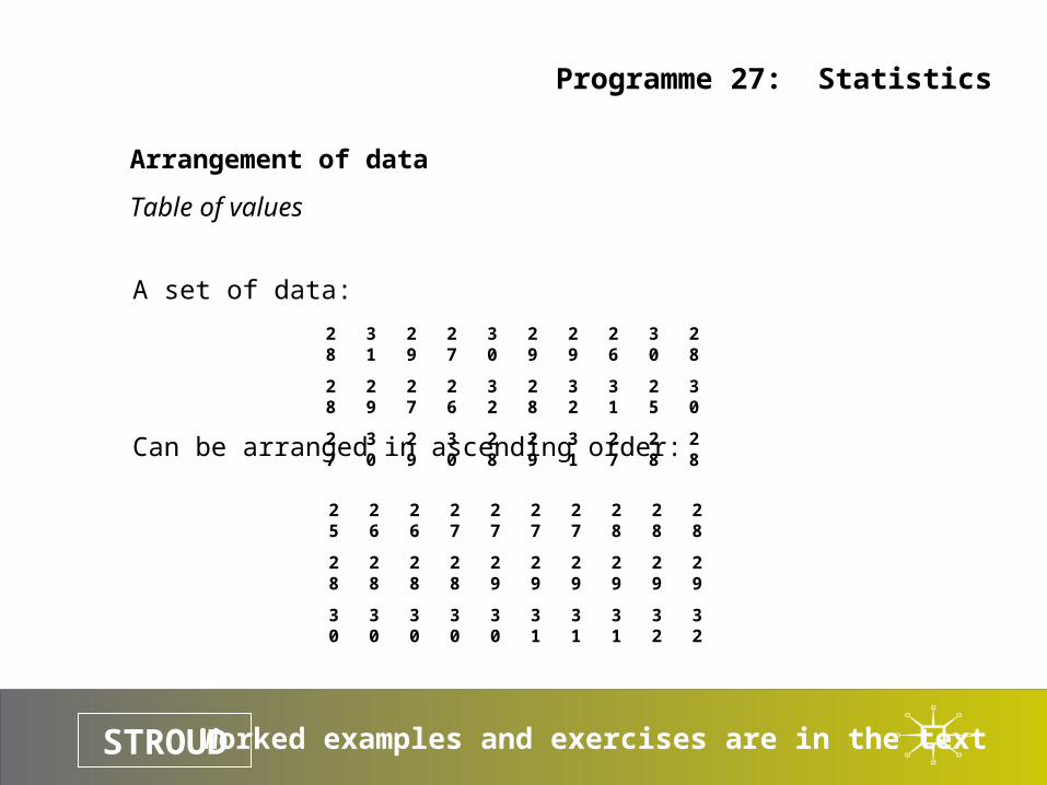
A set of data:
Can be arranged in ascending order:
28 31 29 27 30 29 29 26 30 28
28 29 27 26 32 28 32 31 25 30
27 30 29 30 28 29 31 27 28 28
25 26 26 27 27 27 27 28 28 28
28 28 28 28 29 29 29 29 29 29
30 30 30 30 30 31 31 31 32 32
Worked examples and exercises are in the textSTROUD
Programme 27: Statistics
Arrangement of data
Table of values
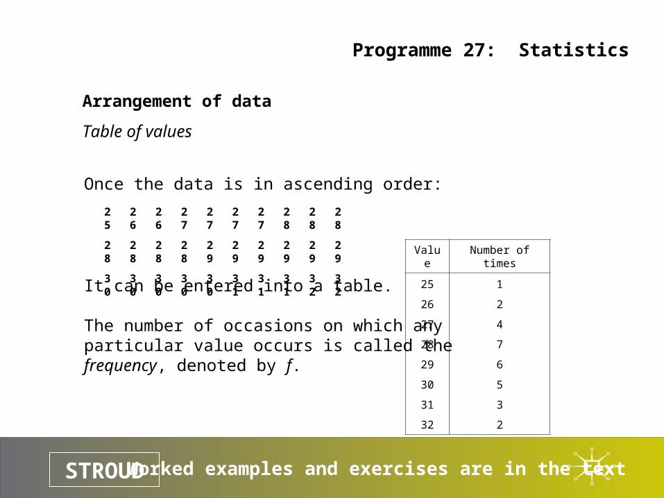
Once the data is in ascending order:
It can be entered into a table.
The number of occasions on which anyparticular value occurs is called the frequency, denoted by f.
25 26 26 27 27 27 27 28 28 28
28 28 28 28 29 29 29 29 29 29
30 30 30 30 30 31 31 31 32 32 Value Number of times
25 1
26 2
27 4
28 7
29 6
30 5
31 3
32 2
Worked examples and exercises are in the textSTROUD
Programme 27: Statistics
Arrangement of data
Tally diagram
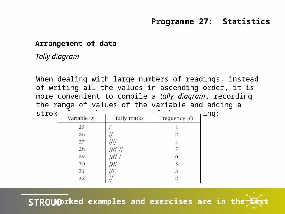
When dealing with large numbers of readings, instead of writing all the values in ascending order, it is more convenient to compile a tally diagram, recording the range of values of the variable and adding a stroke for each occurrence of that reading:
Worked examples and exercises are in the textSTROUD
Programme 27: Statistics
Arrangement of data
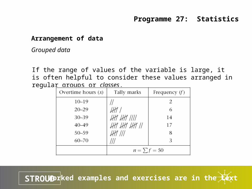
Grouped data
If the range of values of the variable is large, it is often helpful to consider these values arranged in regular groups or classes.
Worked examples and exercises are in the textSTROUD
Programme 27: Statistics
Arrangement of data
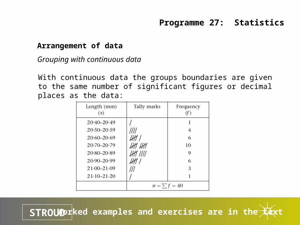
Grouping with continuous data
With continuous data the groups boundaries are given to the same number of significant figures or decimal places as the data:
Worked examples and exercises are in the textSTROUD
Programme 27: Statistics
Arrangement of data
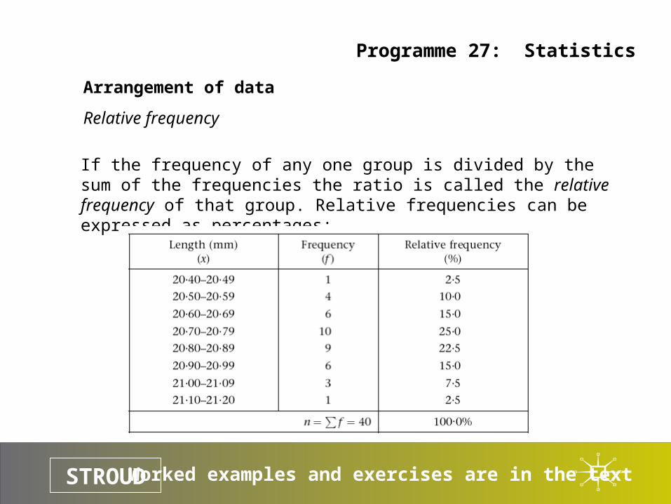
Relative frequency
If the frequency of any one group is divided by the sum of the frequencies the ratio is called the relative frequency of that group. Relative frequencies can be expressed as percentages:
Worked examples and exercises are in the textSTROUD
Programme 27: Statistics
Arrangement of data
Rounding off data
If the value 21.7 is expressed to two significant figures, the result is rounded up to 22. similarly, 21.4 is rounded down to 21.
To maintain consistency of group boundaries, middle values will always be rounded up. So that 21.5 is rounded up to 22 and 42.5 is rounded up to 43.
Therefore, when a result is quoted to two significant figures as 37 on a continuous scale this includes all possible values between:
36.50000… and 37.49999…
Worked examples and exercises are in the textSTROUD
Programme 27: Statistics
Arrangement of data
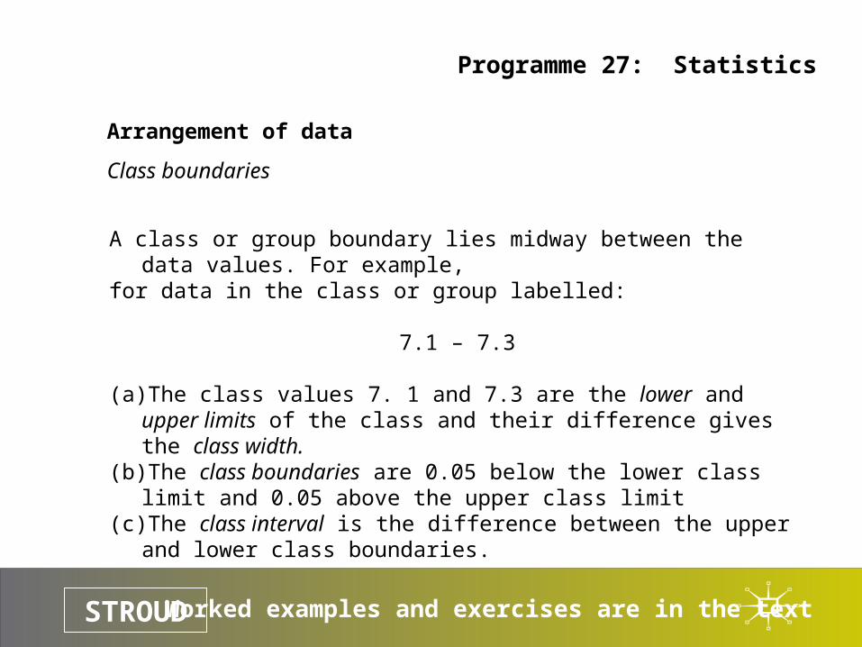
Class boundaries
A class or group boundary lies midway between the data values. For example, for data in the class or group labelled:
7.1 – 7.3
(a) The class values 7. 1 and 7.3 are the lower and upper limits of the class and their difference gives the class width.
(b) The class boundaries are 0.05 below the lower class limit and 0.05 above the upper class limit
(c) The class interval is the difference between the upper and lower class boundaries.
Worked examples and exercises are in the textSTROUD
Programme 27: Statistics
Arrangement of data
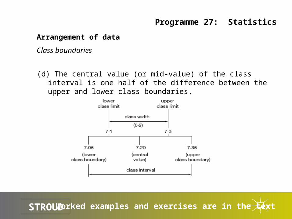
Class boundaries
(d) The central value (or mid-value) of the class interval is one half of the difference between the upper and lower class boundaries.
Worked examples and exercises are in the textSTROUD
Programme 27: Statistics
Introduction
Arrangement of data
Histograms
Measure of central tendency
Dispersion
Frequency polygons
Frequency curves
Normal distribution curve
Standardized normal curve
Worked examples and exercises are in the textSTROUD
Programme 27: Statistics
Histograms
Frequency histogram
Relative frequency histogram
Worked examples and exercises are in the textSTROUD
Programme 27: Statistics
Histograms
Frequency histogram
A histogram is a graphical representation of a frequency distribution in which vertical rectangular blocks are drawn so that:
(a) the centre of the base indicates the central value of the class and
(b) the area of the rectangle represents the class frequency
Worked examples and exercises are in the textSTROUD
Programme 27: Statistics
Histograms
Frequency histogram
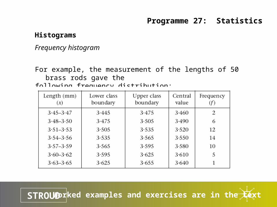
For example, the measurement of the lengths of 50 brass rods gave the following frequency distribution:
Worked examples and exercises are in the textSTROUD
Programme 27: Statistics
Histograms
Frequency histogram
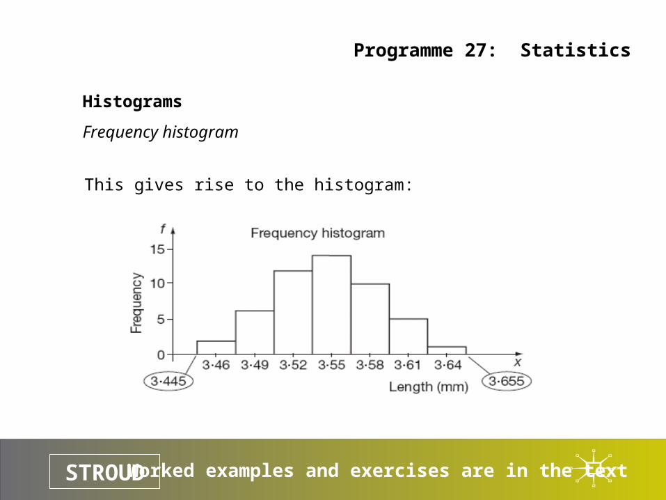
This gives rise to the histogram:
Worked examples and exercises are in the textSTROUD
Programme 27: Statistics
Histograms
Relative frequency histogram
A relative frequency histogram is identical in shape to the frequency histogram but differs in that the vertical axis measures relative frequency.
Worked examples and exercises are in the textSTROUD
Programme 27: Statistics
Introduction
Arrangement of data
Histograms
Measure of central tendency
Dispersion
Frequency polygons
Frequency curves
Normal distribution curve
Standardized normal curve
Worked examples and exercises are in the textSTROUD
Programme 27: Statistics
Measure of central tendency
Mean
Mode of a set of data
Mode of a grouped frequency distribution
Median of a set of data
Median with grouped data
Worked examples and exercises are in the textSTROUD
Programme 27: Statistics
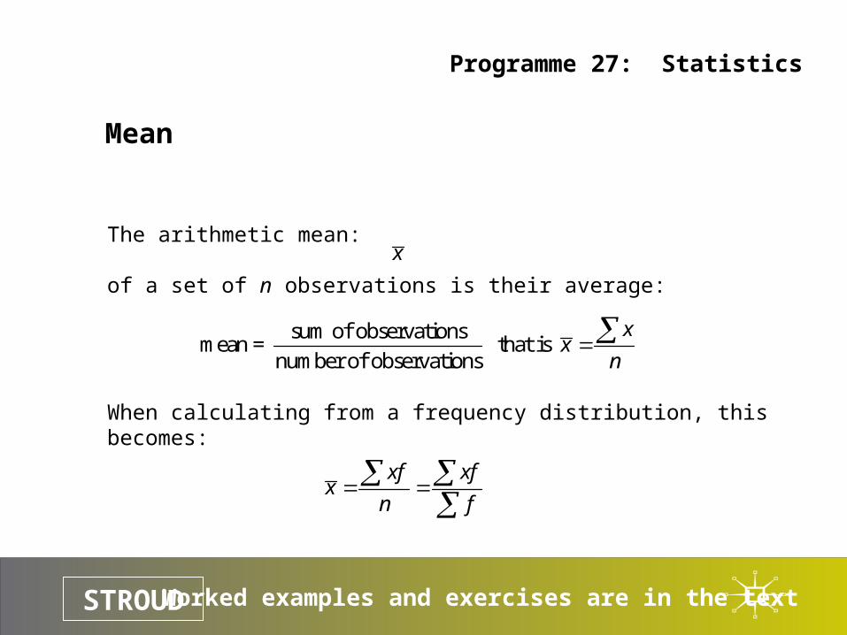
Mean
The arithmetic mean:
of a set of n observations is their average:
When calculating from a frequency distribution, this becomes:
x
sum of observationsmean = that is
number of observations
xx
n
xf xfx
n f
Worked examples and exercises are in the textSTROUD
Programme 27: Statistics
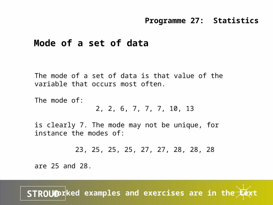
Mode of a set of data
The mode of a set of data is that value of the variable that occurs most often.
The mode of:2, 2, 6, 7, 7, 7, 10, 13
is clearly 7. The mode may not be unique, for instance the modes of:
23, 25, 25, 25, 27, 27, 28, 28, 28
are 25 and 28.
Worked examples and exercises are in the textSTROUD
Programme 27: Statistics
Mode of a grouped frequency distribution
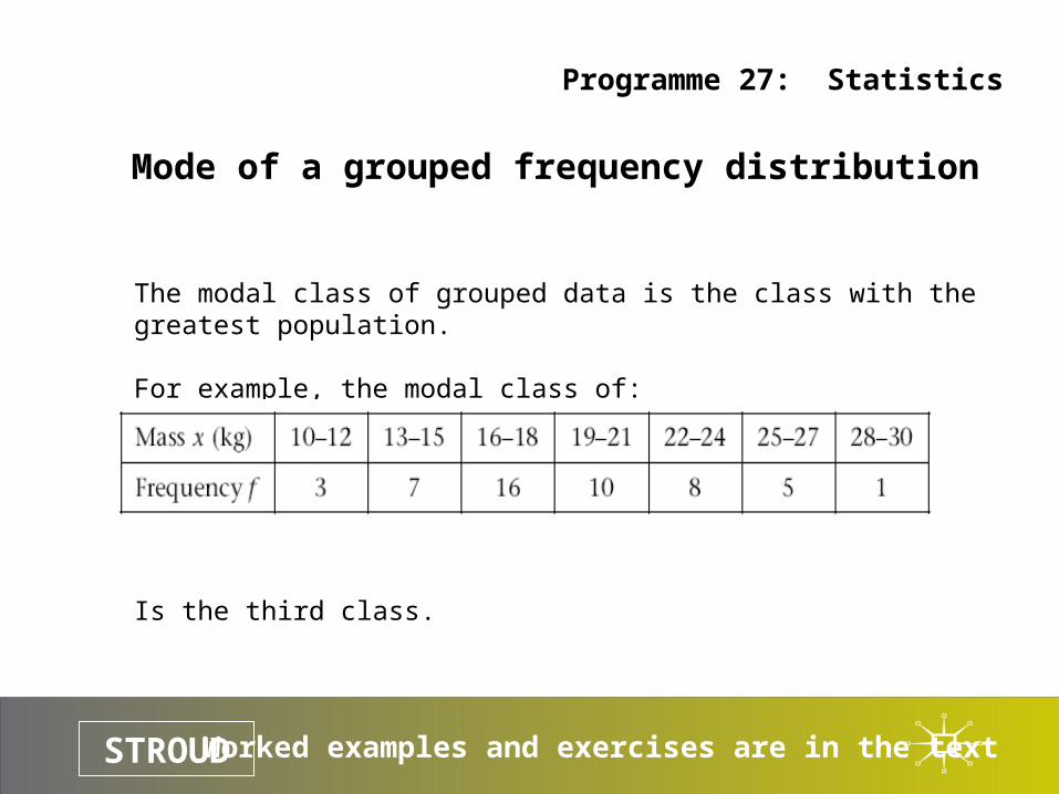
The modal class of grouped data is the class with the greatest population.
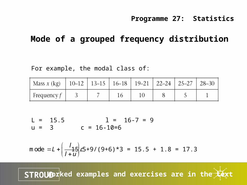
For example, the modal class of:
Is the third class.
Worked examples and exercises are in the textSTROUD
Programme 27: Statistics
Mode of a grouped frequency distribution
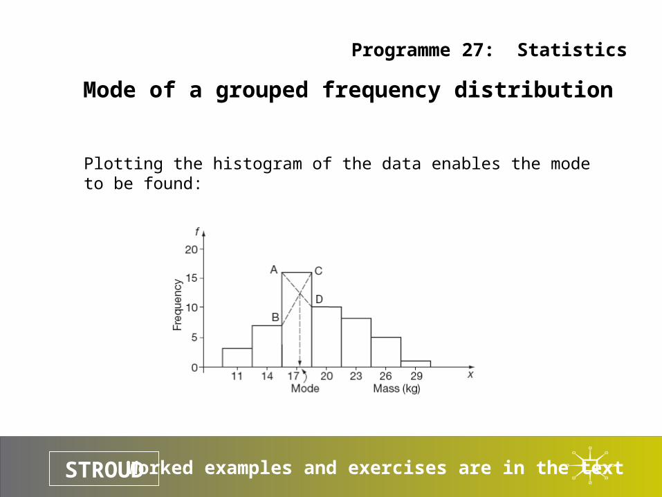
Plotting the histogram of the data enables the mode to be found:
Worked examples and exercises are in the textSTROUD
Programme 27: Statistics
Mode of a grouped frequency distribution
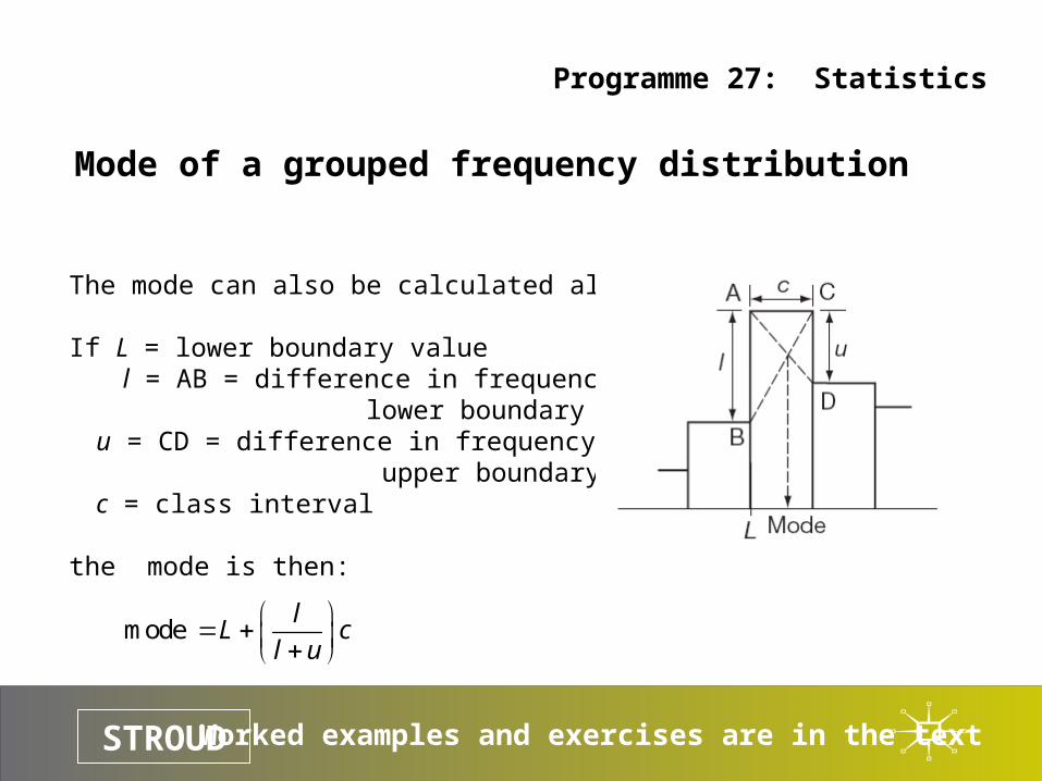
The mode can also be calculated algebraically:
If L = lower boundary value l = AB = difference in frequency on the lower boundary u = CD = difference in frequency on the upper boundary c = class interval
the mode is then:
mode l
L cl u
Worked examples and exercises are in the textSTROUD
Programme 27: Statistics
Mode of a grouped frequency distribution
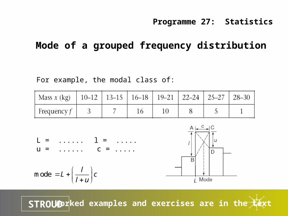
For example, the modal class of:
L = ...... l = .....u = ...... c = .....
mode l
L cl u
Worked examples and exercises are in the textSTROUD
Programme 27: Statistics
Mode of a grouped frequency distribution
For example, the modal class of:
L = 15.5 l = 16-7 = 9u = 3 c = 16-10=6
mode l
L cl u
15.5+9/(9+6)*3 = 15.5 + 1.8 = 17.3
Worked examples and exercises are in the textSTROUD
Programme 27: Statistics
Median of a set of data
The median is the value of the middle datum when the data is arranged in ascending or descending order.
If there is an even number of values the median is the average of the two middle data.
Worked examples and exercises are in the textSTROUD
Programme 27: Statistics
Median with grouped data
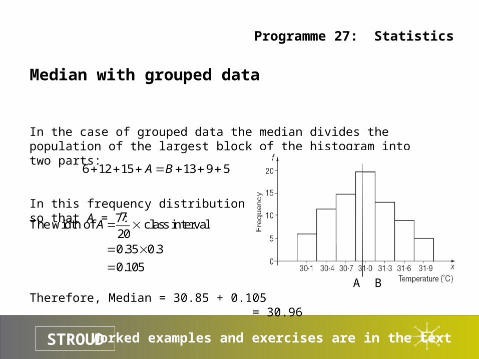
In the case of grouped data the median divides the population of the largest block of the histogram into two parts:
In this frequency distribution A + B = 20so that A = 7:
Therefore, Median = 30.85 + 0.105 = 30.96
6 12 15 13 9 5A B
7The width of class interval
200.35 0.3
0.105
A
A B
Worked examples and exercises are in the textSTROUD
Programme 27: Statistics
Introduction
Arrangement of data
Histograms
Measure of central tendency
Dispersion
Frequency polygons
Frequency curves
Normal distribution curve
Standardized normal curve
Worked examples and exercises are in the textSTROUD
Programme 27: Statistics
Dispersion
Range
Standard deviation
Alternative formula for the standard deviation
Worked examples and exercises are in the textSTROUD
Programme 27: Statistics
Dispersion
Range
The mean, mode and median give important information about the central tendency of data but they do not tell anything about the spread or dispersion about the centre.
For example, the two sets of data:
26, 27, 28 ,29 30 and 5, 19, 20, 36, 60
both have a mean of 28 but one is clearly more tightly arranged about the mean than the other. The simplest measure of dispersion is the range – the difference between the highest and the lowest values.
Worked examples and exercises are in the textSTROUD
Programme 27: Statistics
Dispersion
Standard deviation
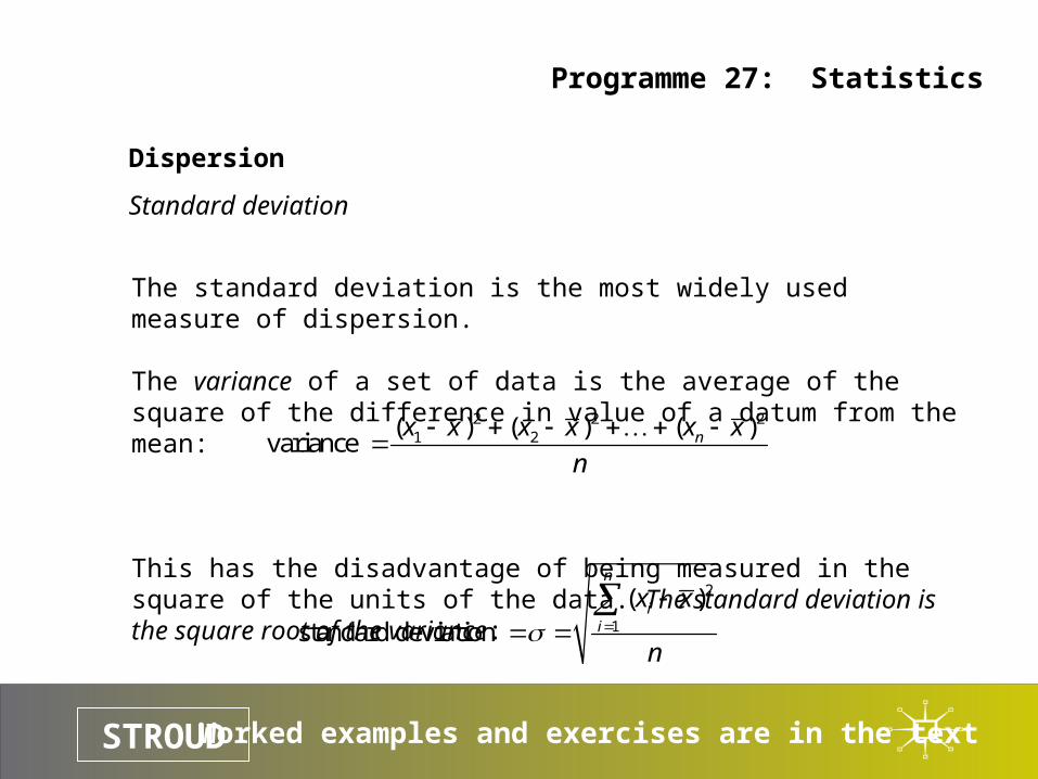
The standard deviation is the most widely used measure of dispersion.
The variance of a set of data is the average of the square of the difference in value of a datum from the mean:
This has the disadvantage of being measured in the square of the units of the data. The standard deviation is the square root of the variance:
2 2 21 2( ) ( ) ( )
variance nx x x x x x
n
2
1
( )standard deviation
n
ii
x x
n
Worked examples and exercises are in the textSTROUD
Programme 27: Statistics
Dispersion
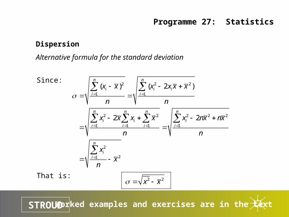
Alternative formula for the standard deviation
Since:
That is:
2 2 2
1 1
2 2 2 2 2
1 1 1 1
2
21
( ) ( 2 )
2 2
n n
i i ii i
n n n n
i i ii i i i
n
ii
x x x x x x
n n
x x x x x nx nx
n n
xx
n
2 2x x