WHOI-2010-05

Woods Hole Oceanographic Institution

Stratus 10Tenth Setting of the Stratus Ocean Reference Station

Cruise RB-10-01January 2 - January 30, 2010

Charleston, South Carolina - Valparaiso, Chileby

Sebastien Bigorre,1 Robert Weller,1 Jeff Lord,1 Nancy Galbraith,1 Sean Whelan,1

Chris Zappa,2 William Otto,3 Jessica Ram,4 Raul Vasquez,5 Diane Suhm6

Woods Hole Oceanographic Institution, Woods Hole, Massachusetts 02543

May 2010

Technical Report

Funding was provided by the National Oceanic and Atmospheric Administration under Grant No. NA17RJ1223 for the Cooperative Institute for Climate and Ocean Research (CICOR).

Approved for public release; distribution unlimited.

UP

PE

R O

C

EA

N P R O CE

S

SE

S

GR

OU

P

Upper Ocean Processes GroupWoods Hole Oceanographic InstitutionWoods Hole, MA 02543UOP Technical Report 2010-02

1 Woods Hole Oceanographic Institution, Woods Hole, MA 2 Lamont Dohery Earth Observatory, NY3 NOAA, Earth System Research Laboratory, CO 4 Colorado State University, Boulder, CO5 Dirección de Hidrografia y Navegación, Peruvian Navy, Perú6 Volunteer, WHOI

WHOI-2010-05

Stratus 10 Tenth Setting of the Stratus Ocean Reference Station

Cruise RB-10-01 January 2 -January 30, 2010

Charleston, South Carolina - Valparaiso, Chile

by

Sebastien Bigorre, Robert Weller, Jeff Lord, Nancy Galbraith, Sean Whelan, Chris Zappa, William Otto,Jessica Ram, Raul Vasquez, Diane Suhm

Woods Hole Oceanographic Institution Woods Hole, Massachusetts 02543

May 2010

Technical Report

Funding was provided by the National Oceanic and Atmospheric Administration under grant No. NA17RJ1223 and the Cooperative Institute for Climate and Ocean Research (CICOR).

Reproduction in whole or in part is permitted for any purpose of the United States Government. This report should be cited as Woods Hole Oceanographic Institution Tech.

Report, WHOI-2010-05.

Approved for public release; distribution unlimited.

Approved for Distribution:

Robert A. Weller, Chair

Department of Physical Oceanography

ii

iii

Abstract The Ocean Reference Station at 20°S, 85°W under the stratus clouds west of northern Chile is being maintained to provide ongoing climate-quality records of surface meteorology, air-sea fluxes of heat, freshwater, and momentum, and of upper ocean temperature, salinity, and velocity variability. The Stratus Ocean Reference Station (ORS Stratus) is supported by the National Oceanic and Atmospheric Administration’s (NOAA) Climate Observation Program. It is recovered and redeployed annually, with past cruises that have come between October and December. Due to necessary repairs on the electric motors of the ship’s propulsion system, this year the cruise was delayed until January. During the 2009/2010 cruise on the NOAA ship Ronald H. Brown to the ORS Stratus site, the primary activities were the recovery of the Stratus 9 WHOI surface mooring that had been deployed in October 2008, deployment of a new (Stratus 10) WHOI surface mooring at that site, in-situ calibration of the buoy meteorological sensors by comparison with instrumentation installed on the ship by staff of the NOAA Earth System Research Laboratory (ESRL), and collection of underway and on station oceanographic data to continue to characterize the upper ocean in the stratus region. Both underway CTD (UCTD) profiles and Vertical Microstructure Profiles (VMP) were collected along the track and during surveys dedicated to investigating eddy variability in the region. Surface drifters were also launched along the track. The intent was also to visit a buoy for the Pacific tsunami warning system maintained by the Hydrographic and Oceanographic Service of the Chilean Navy (SHOA). This DART (Deep-Ocean Assessment and Reporting of Tsunami) buoy had been equipped with IMET sensors and subsurface oceanographic instruments, and a recovery and replacement of the IMET sensors was planned. However, the DART buoy broke free from its mooring on January 3rd and was recovered by the Chilean navy; the work done at that site during this cruise was the recovery of the bottom pressure unit.

iv

v

TABLE OF CONTENTS Abstract ............................................................................................................................. iii Table of Contents ............................................................................................................ v-vi List of Figures ............................................................................................................. vii-viii List of Tables ................................................................................................................... viii I. Introduction ...............................................................................................................1 A. Timeline ................................................................................................................1 B. Background and Purpose ......................................................................................4

II. Cruise preparations ..................................................................................................6 A. Sensor Evaluation and Burn-in .............................................................................6 B. Staging and Loading in Charleston .....................................................................11 C. Buoy Spin............................................................................................................12

III. Stratus 10 Mooring ................................................................................................13 A. Mooring Design ..................................................................................................13 B. Buoy Instrumentation..........................................................................................15 1) ASIMET .........................................................................................................16 2) Sea Surface Temperature ................................................................................17 3) Air Temperature and Relative Humidity ........................................................18 4) Precipitation ....................................................................................................18 5) Shortwave radiation ........................................................................................18 6) Longwave radiation ........................................................................................18 7) Barometric pressure ........................................................................................18 8) Wind ...............................................................................................................18 9) Subsurface Argos Transmitter ........................................................................19 10) Telemetry ......................................................................................................19 11) PCO2 .............................................................................................................19 12) Wave Package ...............................................................................................19 C. Subsurface Instrumentation ................................................................................19 1) VMCMs ..........................................................................................................21 2) RDI Acoustic Doppler Current meter .............................................................21 3) Nortek .............................................................................................................22 4) Sontek Argonaut MD Current Meter ..............................................................22 5) Aanderaa RCM 11s ........................................................................................22 6) Aanderaa Seaguard RCM ...............................................................................22

7) SBE-39 Temperature Recorder ......................................................................22 8) SBE-37 Microcat Conductivity and Temperature Recorder ..........................22 9) SBE-16 Seacat Conductivity and Temperature Recorder ..............................22 10) Brancker XR-420 Temperature and Conductivity Recorder ........................23 11) Acoustic Release...........................................................................................23 D. Current Meter Setup ............................................................................................23 E. Antifouling Coatings ...........................................................................................24 F. Mooring Operations. ...........................................................................................25 1) Deployment ....................................................................................................25 2) Anchor Survey ................................................................................................30

vi

G. Instrument Intercomparisons ...............................................................................31 IV. Stratus 9 Mooring ...................................................................................................37 A. Recovery .............................................................................................................37 B. Mooring Failure ..................................................................................................40 C. Stratus 9 Data Return ..........................................................................................41 1) Status Upon Recovery ....................................................................................41 2) Data Return .....................................................................................................45 D. Instrument Intercomparisons ..............................................................................52 E. Stratus 9 Anti-Fouling Performance ...................................................................59 V. Ancillary Projects ....................................................................................................62 A. Underway Conductivity Temperature Depth (UCTD) .......................................62 1) Operation ........................................................................................................62 2) CTD Sensor Specifications .............................................................................63 3) Data Processing ..............................................................................................63 4) UCTD Results.................................................................................................67 B. Vertical Microstructure Profiler (VMP) .............................................................68 C. Ridge Survey .......................................................................................................73 D. Drifter Deployments ...........................................................................................74 E. CTD casts ............................................................................................................78 F. Atmospheric Observations ..................................................................................81 1) Weather ...........................................................................................................81 2) WHOI turbulent flux sensor ...........................................................................82 3) Earth System Research Laboratory (ESRL) Observations .............................82 G. DART ..................................................................................................................87 1) Overview ........................................................................................................87 2) BPR Recovery ................................................................................................89 H. ADCP .................................................................................................................91 I. Student Note (Jessica Ram) ................................................................................92 Thanks and Acknowledgments .......................................................................................94

References .........................................................................................................................94

Appendix 1: Buoy Spins ..................................................................................................95 Appendix 2: Subsurface Seabird Recorders Setup ........................................................103 Appendix 3: Acoustic Current Meters Setup ................................................................107 Appendix 4: VMCM Setup .............................................................................................108 Appendix 5: Stratus 10 Mooring Log .............................................................................111 Appendix 6: Stratus 9 Mooring Diagram ........................................................................118 Appendix 7: Stratus 9 Mooring Log ...............................................................................120 Appendix 8: VMP Pre/post Calibrations for Stratus 2008/2010 ...................................128

vii

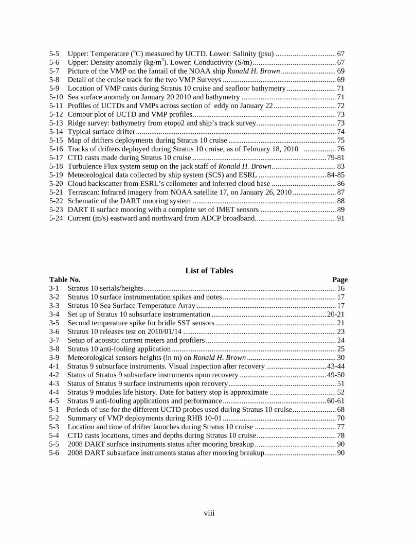
List of Figures Fig No. Page 1-1 Stratus 10 cruise itinerary from Charleston, South Carolina to Valparaiso, Chile ................. 4 2-1 Air temperature as of end of burn-in period ........................................................................... 7 2-2 Air relative humidity as of end of burn-in period .................................................................. 7 2-3 Wind speed as of end of burn-in period ................................................................................. 8 2-4 Wind direction as of end of burn-in period ............................................................................ 8 2-5 Longwave radiation as of end of burn-in period .................................................................... 9 2-6 Shortwave radiation as of end of burn-in period .................................................................... 9 2-7 Barometric pressure as of end of burn-in period .................................................................. 10 2-8 Burnin time series for final ASIMET systems on Stratus10 ................................................ 11 2-9 Buoy spin on Stratus 10 buoy .............................................................................................. 12 3-1 Representation of Stratus 9 ASIMET buoy .......................................................................... 13 3-2 Stratus 10 mooring diagram ................................................................................................. 14 3-3 Seabeam bathymetric survey and deployment track for Stratus 10 ..................................... 27 3-4 Ship deployment track and survey points ............................................................................ 30 3-5 Stratus 10 anchor survey details ........................................................................................... 31 3-6 Outboard profile of the NOAA Ship Ronald H. Brown ....................................................... 32 3-7 Inboard profile of the NOAA Ship Ronald H. Brown .......................................................... 32 3-8 Sea surface temperature. Ships values adjusted to skin value, buoy data ............................ 33 3-9 Wind speed. Zbuoy refers to adjustment to height of sensor on buoy .................................... 33 3-10 Wind direction (oceanographic convention) ........................................................................ 34 3-11 Air temperature. Zbuoy refers to adjustment to height of sensor on buoy .............................. 34 3-12 Air specific humidity. Zbuoy refers to adjustment to height of sensor on buoy ..................... 35 3-13 Downward solar radiation .................................................................................................... 35 3-14 Downward longwave radiation ............................................................................................ 36 3-15 Barometric pressure (ship data adjusted to buoy sensor height) .......................................... 36 4-1 First clump of wire and instruments to be hauled to the surface .......................................... 38 4-2 Broken stainless steel load bar on the 8.4 m dual Nortek instruments ................................. 40 4-3a Picture of RCM-11 recovered .............................................................................................. 41 4-3b Picture of Sontek Argonaut-MD recovered ......................................................................... 41 4-3c Picture of Nortek AS ADCM recovered .............................................................................. 42 4-3d Picture of SBE-39 recovered ................................................................................................ 42 4-4 Surface ASIMET one-minute data from loggers 4 and 15 on Stratus 9 .......................... 45-46 4-5 Subsurface temperature data return on Stratus 9 .................................................................. 47 4-6 Data return from VMCMs and Aanderaa RCM on Stratus 9 ............................................... 47 4-7 Ship and Stratus 9 buoy data inter-comparison on January 19th. Air temperature. .............. 53 4-8 As in Figure 4-7. Specific humidity ..................................................................................... 54 4-9 As in Figure 4-7. Shortwave downward radiation ............................................................... 54 4-10 As in Figure 4-7. Longwave downward radiation ................................................................ 55 4-11 As in Figure 4-7. Sea surface temperature ........................................................................... 55 4-12 Water temperature (°C) on October 26 2008 ....................................................................... 56 4-13 As in Figure 4-12, except on June 21 2009 .......................................................................... 56 4-14 As in Figure 4-12, except on November 21 2009 ................................................................ 57 4-15 SST from SBE37 on buoy’s bridle ....................................................................................... 57 4-16 As in Figure 4-15 but for conductivity ................................................................................. 58 4-17 As in Figure 4-15 but for salinity ......................................................................................... 58 5-1 UCTD Assembled ................................................................................................................ 62 5-2 Pressure time series during CTD/UCTD comparison .......................................................... 64 5-3 CTD/UCTD comparison ...................................................................................................... 65 5-4 Two UCTDs done just before and after CTD cast ............................................................... 66

viii

5-5 Upper: Temperature (oC) measured by UCTD. Lower: Salinity (psu) ................................ 67 5-6 Upper: Density anomaly (kg/m3). Lower: Conductivity (S/m) ............................................ 67 5-7 Picture of the VMP on the fantail of the NOAA ship Ronald H. Brown ............................. 69 5-8 Detail of the cruise track for the two VMP Surveys ............................................................ 69 5-9 Location of VMP casts during Stratus 10 cruise and seafloor bathymetry .......................... 71 5-10 Sea surface anomaly on January 20 2010 and bathymetry .................................................. 71 5-11 Profiles of UCTDs and VMPs across section of eddy on January 22 ................................. 72 5-12 Contour plot of UCTD and VMP profiles ............................................................................ 73 5-13 Ridge survey: bathymetry from etopo2 and ship’s track survey .......................................... 73 5-14 Typical surface drifter .......................................................................................................... 74 5-15 Map of drifters deployments during Stratus 10 cruise ......................................................... 75 5-16 Tracks of drifters deployed during Stratus 10 cruise, as of February 18, 2010 ................. 76 5-17 CTD casts made during Stratus 10 cruise ....................................................................... 79-81 5-18 Turbulence Flux system setup on the jack staff of Ronald H. Brown .................................. 83 5-19 Meteorological data collected by ship system (SCS) and ESRL .................................... 84-85 5-20 Cloud backscatter from ESRL’s ceilometer and inferred cloud base .................................. 86 5-21 Terrascan: Infrared imagery from NOAA satellite 17, on January 26, 2010 ....................... 87 5-22 Schematic of the DART mooring system ............................................................................ 88 5-23 DART II surface mooring with a complete set of IMET sensors ........................................ 89 5-24 Current (m/s) eastward and northward from ADCP broadband. .......................................... 91

List of Tables Table No. Page 3-1 Stratus 10 serials/heights ...................................................................................................... 16 3-2 Stratus 10 surface instrumentation spikes and notes ............................................................ 17 3-3 Stratus 10 Sea Surface Temperature Array .......................................................................... 17 3-4 Set up of Stratus 10 subsurface instrumentation ............................................................. 20-21 3-5 Second temperature spike for bridle SST sensors ................................................................ 21 3-6 Stratus 10 releases test on 2010/01/14 ................................................................................. 23 3-7 Setup of acoustic current meters and profilers ..................................................................... 24 3-8 Stratus 10 anti-fouling application ....................................................................................... 25 3-9 Meteorological sensors heights (in m) on Ronald H. Brown ............................................... 30 4-1 Stratus 9 subsurface instruments. Visual inspection after recovery ................................ 43-44 4-2 Status of Stratus 9 subsurface instruments upon recovery .............................................. 49-50 4-3 Status of Stratus 9 surface instruments upon recovery ......................................................... 51 4-4 Stratus 9 modules life history. Date for battery stop is approximate ................................... 52 4-5 Stratus 9 anti-fouling applications and performance ....................................................... 60-61 5-1 Periods of use for the different UCTD probes used during Stratus 10 cruise ....................... 68 5-2 Summary of VMP deployments during RHB 10-01 ............................................................ 70 5-3 Location and time of drifter launches during Stratus 10 cruise ........................................... 77 5-4 CTD casts locations, times and depths during Stratus 10 cruise .......................................... 78 5-5 2008 DART surface instruments status after mooring breakup ........................................... 90 5-6 2008 DART subsurface instruments status after mooring breakup...................................... 90

1

I. Introduction

A. Timeline

The cruise began in Charleston, South Carolina, on January 2, 2010, and ended in Valparaiso, Chile, on January 30, 2010. An overview of the chronology of the cruise is provided below. Jan 2. Departure from Charleston at 10:00 EST. Northwest wind. Jan 3. Stopped near Jacksonville, Florida, to pick up technician for inspection of ship’s engine sparking. Cold weather, northwest wind. Jan 4. Stopped near Key Biscayne to drop off technician. Setup pCO2 system. Jan 5. Chief scientist presented results from the Stratus mooring data. Passed Florida Keys, turned south and crossed the Loop current. Swell from the west, choppy sea, cloudy then clearing in evening. Fire alarm. Passed Cuba’s western tip at night. Jan 6. Entered Caribbean Sea (Yucatan Basin). UCTD training 09:00 EST. Jan 7. (17°27’N, 81°44’W) at 08:18 EST. Dumped data from buoy loggers and standalones. Spiked subsurface temperature sensors, including Norteks. Jan 8. (13°51’N, 80°36’W) at 07:00 EST. Replaced HRH231 (L-2) with spare HRH223 and PRC208 (SA) with spare PRC205 (including electronic unit) at 12:32 EST. Started VMCMs around 14:00 EST. Jan 9. (9°35’N, 79°56’W) at 07:30 EST. Near Cristobal, Panama canal entrance. Ship’s speed 7 knots, water depth 48m. Turned off pCO2 system for safety on deck (water flushing stopped). Ship’s data underway system shut down (water pump), 08:30 EST. Erased memory card on WAMDAS, 13:30 EST. Pulled seasnake out of water. Entered Panama Canal 16:30 EST. Entered Miraflores locks 22:00 EST. Jan 10. Anchored in Rodman, Panama. Foreign observers and remaining scientists arrived on board 09:00 EST. Departed Rodman, 09:30 EST. Seasnake back in water 10:00 EST. Safety briefing and introduction for new personnel 11:00 EST. Science meeting 13:00 EST. Jan 11. (3°58’N, 80°51’W) at 08:20 EST. Training mooring operation on fantail. Jan 12. Entered Peruvian EEZ at 23:43 EST. Jan 13. UCTD started around 00:00 EST; 1 cast per hour. (4°59’S, 83°43’W) at 09:00 EST. Biofouling painting. Exit Peruvian EEZ (6°56.75’S, 84°21.03’W) at 19:48 EST. Jan 14. UCTD continues. CTD cast at 1500m depth, with acoustic releases attached for ping test (result OK). Drifter 1 (ID 90189) deployed at (10°30.047’N, 84°54.829’W) at 21:42 UTC.

2

Jan 15. UCTD continues. Drifter 2 (ID 90188) launched at 08:17 UTC at (12°31.327’S, 85°02.491’W). Drifter 3 (ID 90170) launched at 16:15 UTC at (14°00.878’S, 85°09.085’W). Jan 16. UCTD continues. Entering high pressure eddy. Launched drifter 4 (ID 90194), drifter 5 (ID 90175). Launched drifters inside eddy: drifter 6 (ID 90186) at (18°29.89’S, 85°29.38’W) at 15:46 UTC, drifter 17 (ID 90185) launched at (18°58.03’S, 85°31.78’W) at 18:16 UTC. Drifter 18 (ID 90187) launched at (19°14.74’S, 85°33’W) at 19:46 UTC. Arrived at Stratus 9 mooring site at 16:00 EST for quick visual check. Jan 17. Stratus 10 deployment (07:30 to 15:00 EST). Anchor survey (4 points). Three UCTDs at survey points. Parked downwind of Stratus 10 mooring at 22:00 EST for 24 hours of instrument inter-comparison, facing wind (about 140° heading). Jan 18. Deep CTD (4000m) next to Stratus 10 site at 15:00 UTC. Shallow CTD and Nortek test for Chris Zappa. UCTD comparison with CTD (UCTD probe 29 has a high bias in conductivity). SST experiment. Fire/abandon ship drills. Started “Volume” experiment at 20:30 EST: VMPs and UCTDs around stratus 10, in a square with 6 nm length sides. Jan 19. Volume experiment ends at 05:00 EST. Rain (maybe for the first time during this cruise) in the early morning. Move to Stratus 9 and keep station at 07:00 EST for next 24 hours. Deep CTD (4000m, with cups) from 13:00 to 15:00 EST. Prepare plan for eddy survey. Jan 20. Anchor released at 06:30 EST. Glass balls on deck at 08:30. Buoy parted from mooring. Slow recovery due to high tension on line. 20:00 EST, all the mooring line is on deck. Many instruments broken, entangled together, covered with mud. Some fishing gear. Heading northwest (330° true) towards drifting buoy. Jan 21. Stratus 9 drifting buoy recovered. Failure point identified at welding point on load bar of shallow microstructure Nortek. Cleaned instruments and buoy. Started eddy survey with VMP/UCTD sections. Jan 22. Finished first transect (SW to NE diagonal). Interruption of VMP due to damaged wire, UCTD continues. Longitudinal transect NE to NW. Jeff and Chris cut damaged wire and reconnected VMP. VMP resumes for diagonal transect (NW to SE), with one UCTD between stations. Jan 23. Finished last transect of eddy survey with VMP/UCTD. Drifter 7 (90173) launched at 10:10 UTC at (19°41.60’S, 83°58.00’W). Drifter 8 (ID 75453) launched at (19°42.00’S, 83°00’W) at 20:06 UTC. Drifter 19 (ID 75456) launched at (19°11.72’S, 85°17.18’W) at 00:54 UTC. Drifter 20 (ID 90172) launched at (19°25.50’S, 85°02’W) at 03:44 UTC. Drifter 21 (ID 90198) launched at (19°38.00’S, 85°49.50’W) at 06:43 UTC. Steamed east towards DART site. Jan 24. Ship time change from EST (UTC-5) to UTC-4. Stopped 10 nm west of seamount (part of Nazca ridge) for 600m VMP cast at 09:00 UTC. Multibeam sonar turned on for bathymetric survey. Second VMP on east side of seamount at 13:00 UTC. Resumed transit east towards DART site. Drifter 9 (ID 90171) launched at (19°40.04’S, 81°59.50’W) at 00:57 UTC. Drifter 10

3

(ID 90197) launched at (19°39.82’S, 80°59.34’W) at 06:07 UTC. Drifter 11 (ID 90174) launched at (19°39.21’S, 80°00’W) at 12:44 UTC. Drifter 12 (ID 90179) launched at (19°38.578’S, 78°59.49’W) at 17:58 UTC. Drifter 13 (ID 75455) launched at (19°38.01’S, 78°00’W) at 22:53 UTC. Half hour UCTDs continue. Jan 25. Calm sea, no wind and sunny, northwest swell. Arrived at DART site. Released BPR of DART buoy from its anchor. Recovered BPR. CTD (1000m). Drifter 14 (ID 90176) launched at (19°37.316’S, 76°59.106’W) at 03:55 UTC. Drifter 15 (ID 90178) launched at (19°36.7’S, 75°59.18’W) at 09:03 UTC. Drifter 16 (ID 90177) launched at (19°36.127’S, 75°01.004’W) at 13:56 UTC. One hour UCTDs. Ship’s speed reduced to 7 kn, heading 170◦ true. Jan 26. Calm sea, northwest swell, wind and waves picked up in early afternoon. Drifter 22 (ID 75454) launched at (21°30.51’S, 74°20.896’W) at 11:08 UTC. UCTD continues. Entered Chile EEZ at 14:06 (21°53.082’S, 74°16.116’W). Jan 27. UCTD continues. Drifter 23 (ID 75457) launched at (23°30.24’S, 73°53.51’W) at 03:50 UTC. Drifter 24 (ID 90195) launched at (25°29.4’S, 73°25.97’W) at 19:57 UTC. Jan 28. Drifter 25 (ID 90196) launched at (27°30’S, 72°58.03’W) at 12:20 UTC. Jan 29. En route to Valparaiso, Chile. UCTD stopped. Ship met data stopped. Jan 30. Enter Valparaiso’s port.

4

Figure 1-1. Stratus 10 cruise itinerary from Charleston, South Carolina, to Valparaiso, Chile.

B. Background and Purpose

The presence of a persistent stratus deck in the subtropical eastern Pacific is the subject of active research in atmospheric and oceanographic science. Its origin and maintenance are still open to discussion. A better understanding of the processes responsible for this system is desirable not only because better understanding of the nature of air-sea interactions in this region is needed, but also because climate models presently have SST fields that are too warm in the eastern South Pacific. There is also the need to collect in-situ data to provide ground truth for remote sensing. The Ocean Reference Station at 20°S, 85°W under the stratus clouds west of northern Chile is being maintained to provide ongoing, climate-quality records of surface meteorology, of air-sea fluxes of heat, freshwater, and momentum, and of upper ocean temperature, salinity, and velocity variability. The Stratus Ocean Reference Station (ORS Stratus) is supported by the National Oceanic and Atmospheric Administration’s (NOAA) Climate Observation Program. It has been recovered and redeployed annually, with cruises that have come between October and December. The cruise described by this report was planned for October 2009. The equipment was shipped to Charleston and loaded on the NOAA Ship Ronald H. Brown in October 2009. Just before the planned sailing date, the cruise was cancelled and repairs made to the electric motors. The cruise was rescheduled for January 2010.

5

During the 2010 cruise of NOAA’s Ronald H. Brown (RHB) to the ORS Stratus site, the primary activities were recovery of the WHOI surface mooring that had been deployed in October 2008, deployment of a new WHOI surface mooring at that site, and in-situ calibration of the buoy meteorological sensors by comparison with the ship’s sensors and with instrumentation put on board by staff of the NOAA Earth System Research Laboratory (ESRL, formerly ETL). The ORS Stratus buoys are equipped with two Improved Meteorological (IMET) systems, which provide surface wind speed and direction, air temperature, relative humidity, barometric pressure, incoming shortwave radiation, incoming longwave radiation, precipitation rate, and sea surface temperature. The buoy is also outfitted with a PCO2 sampling system. The IMET data are made available in near real time using satellite telemetry. The mooring line carries instruments to measure ocean salinity, temperature, and currents. The ESRL instrumentation used during the 2010 cruise included sensors for mean and turbulent surface meteorology. In recent years, collaboration with the Chilean Navy Hydrographic and Oceanographic Service (SHOA) has allowed IMET sensors to be added to a surface buoy at 20°S, 75°W and also for ocean temperature and salinity sensors to be attached to the mooring line of that buoy. Every year the IMET sensors are recovered and replaced, while every two years the ocean sensors are recovered and replaced. When initially planning the cruise to recover Stratus 9 and deploy Stratus 10, the cruise had been scheduled on the Brown for October 2009. The WHOI UOP group loaded all gear, including the buoy on the Brown. However, the cruise was cancelled due to mechanical problems. The cruise was rescheduled as the first cruise for Brown in 2010, so it is labeled RHB 10-01. The ship sailed from Charleston, SC, on January 2, 2010. On January 3, Weller was informed that the DART surface buoy was adrift. A few days later, he learned that the Chilean Navy had the surface buoy and that the mooring line had parted near the surface. This meant that the WHOI oceanographic instrumentation on that mooring was lost. IMET modules that had survived were being taken to Valparaiso. SHOA did ask at that time that the DART BPR be recovered. In preparation for the cruise, Weller had applied for clearance to sample in Peruvian and Chilean waters (Figure 1-1). As a result, the cruise was planned around the beginning of sampling, with the UCTD on entry into Peruvian waters, on the way to the Stratus ORS, mooring work at ORS Stratus, UCTD sampling going east to the DART site, work at the DART site, and UCTD sampling along the track to Valparaiso. A Vertical Microstructure Profiler (VMP) was on board. The reduction of mooring work at DART allowed more time to be devoted to UCTD sampling and VMP deployments. Two surveys were done in the vicinity of the Stratus ORS in support of the VOCALS-related and ongoing science at that site.

6

II. Cruise Preparations

A. Sensor Evaluation and Burn-in

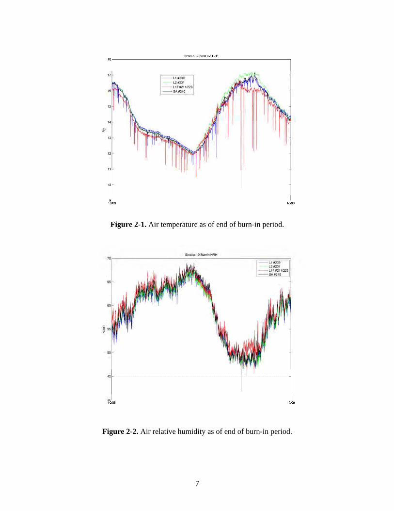
Testing for the ASIMET units deployed on the Stratus 9 buoy began on July 17, when the primary loggers SN L-1 and L-2 were powered up, as well as a spare system L-17, and continued until the instruments were powered down and disassembled for shipping in early October. Plots of the internally recorded 1-minute data from the last data dump of the burn-in period at WHOI is shown in Figures 2-1 to 2-7. The SBE-37 SSTs were found to be functioning as expected and are not plotted here (maximum discrepancy between instruments was observed at mid day when temperature of water in bucket was maximum and was 0.03°C and 0.01 S/m for temperature and conductivity respectively).We usually see some effect of RF noise caused by the Argos PTT transmitters, especially in burn-in data (see for example Figure 2-1); this effect is almost always much less after deployment. Modules that did not perform well during burn-in were replaced. At the end of this initial burn-in period at WHOI, all instruments were performing well when the buoy was disassembled for shipping to Charleston. Once the buoy was reassembled in Charleston, a last phase of the instrument check-out for meteorological sensors began. Using an Alpha Omega Uplink Receiver on the ship, hourly averaged data transmitted by the loggers to the Argos satellite system were continuously monitored until after the buoy was deployed. A data retrieval was also done on January 7 using the RS-232 connections so that 1-minute data from the 2 primary loggers and standalone units was available. It appeared HRH 231 on logger L-2 had a high bias and was therefore replaced by the spare HRH 223 on January 8, while en route to the Panama Canal. Similarly, PRC 208 standalone was replaced by the spare PRC 205 (sensor and electronic unit). Figure 2-8 shows the burnin time series for the final ASIMET systems deployed on Stratus 10, based on hourly averaged data transmitted through Argos telemetry. This shows the effect of the replacement of the HRH unit on Logger 2, to the spare unit HRH223. The humidities are in better agreement after the swap on January 8 (see spike in ATMP and HRH) although there is still a bias visible. Note that the buoy was located on the fantail at this time, which had very heterogeneous conditions because of the wind distortion from the ship and seaspray projections from the port side. These conditions are probably the cause of the apparent diurnal cycle in ATMP from January 8 until Stratus 10 deployment.

7

Figure 2-1. Air temperature as of end of burn-in period.

Figure 2-2. Air relative humidity as of end of burn-in period.

8

F

Figure 2-3. Wind speed as of end of burn-in period.

Figure 2-4. Wind direction as of end of burn-in period.

9

Figure 2-5. Longwave radiation as of end of burn-in period.

Figure 2-6. Shortwave radiation as of end of burn-in period.

10

Figure 2-7. Barometric pressure as of end of burn-in period.

11

Figure 2-8. Burn-in time series for final ASIMET systems on Stratus 10, based on hourly data transmitted through Argos.

B. Staging and Loading in Charleston

In mid-October the equipment was shipped by truck from Woods Hole to Charleston. The equipment was then loaded onboard the NOAA Ship Ronald H. Brown, the tower for the meteorological instruments was mounted on the buoy and the whole assembly loaded on the ship’s deck. The scientific laboratory was also set up. At that point, a problem with the ship’s engines compromised the safety for the coming cruise which was then delayed for 2 ½ months while the ship was being repaired. Most of the equipment was then stored in a container on the main deck. On December 29, 2009, the UOP group arrived in Charleston to resume preparations. A sonic sensor was installed on the bow mast and Hasse rain gauge and Vaisala sensor (VWXT520) installed on O2 deck. The build up of the buoy well and tower was completed, and the system was checked for proper function. The buoy was moved into an empty parking lot to perform a check of the compasses on the buoy’s wind modules (buoy spin, see next section and Appendix 1). Transmissions from the

12

instruments on the buoy were received with an Alpha Omega uplink receiver to check the validity of data as part of the final burn-in. The buoy was then loaded onto the ship. C. Buoy spin

Buoy spins were conducted and were found to meet expectations. The buoy spin is a procedure to check the compasses on the buoy. A visual reference direction is first set using an external compass. The buoy is then oriented successively at 8 different angles and the vanes of the anemometers are visually oriented towards the reference direction, and blocked. Wind is recorded for 15 minutes at the end of which the average compass and wind direction is read. The sum should correspond to the reference heading, within errors due to approximations in orientation, compass precision, and any deformation of the magnetic field due to the buoy metallic structure. A first buoy spin was made in Woods Hole and a second one in Charleston. Buoy spin results are shown in Figure 2-9. See Appendix 1 for the details of the buoy spin.

Stratus 10 Charleston Buoy Spin Deviation

-6

-4

-2

0

2

4

6

8

0 45 90 135 180 225 270 315

Degrees Clockwise Turn

Deg

rees

Dev

iati

on

L-01 Sonic

L-02

SL

Figure 2-9. Buoy spin on Stratus 10 buoy.

13

III. Stratus 10 Mooring

A. Mooring Design

The buoys used in the Stratus project are equipped with surface meteorological instrumentation, including two Improved Meteorological (IMET) systems (see Figure 3-1). The mooring line also carries subsurface instrumentation that measures conductivity and temperature and a selection of acoustic current meters and vector measuring current meters (VMCM). The WHOI mooring is an inverse catenary design utilizing wire rope, chain, nylon and polypropylene line and has a scope of 1.25 (scope is defined as slack length/water depth). The Stratus 10 surface buoy has a 2.7-meter diameter foam buoy with an aluminum tower and rigid bridle. The design of these surface moorings takes into consideration the predicted currents, winds, and sea-state conditions expected during the deployment duration. See Figure 3-2 for the full mooring drawing.

Figure 3-1: Representation of Stratus 9 ASIMET buoy.

14

Figure 3-2. Stratus 10 mooring diagram.

15

B. Buoy Instrumentation

The Air-Sea Interaction Meteorology (ASIMET) system is a suite of meteorological and sea surface sensors that are deployed with different housing and packaging depending on the application. ASIMET modules (one or more sensors plus front-end electronics) may be self-powered and self-logging, connected to a central power supply and logger, or both. Together, these modules measure Air temperature (ATMP), relative humidity (HRH), sea surface temperature and conductivity (SST, SSC), wind speed and direction (WSPD, WDIR), barometric pressure (BPR), shortwave radiation (SWR), longwave radiation (LWR), and precipitation (PRC). These variables are used to compute air-sea fluxes of heat, moisture and momentum using bulk aerodynamic formulas. On buoys, modules are packaged in titanium cylinders that include provisions for batteries and internal logging. Buoy modules are typically deployed in pairs, with 6 meteorological module pairs mounted on the buoy tower and a pair of temperature-conductivity sensors attached to the bridle leg. A central logger records one minute data from all the modules on a common time base, and also creates hourly averaged data that are transmitted to shore via Argos satellite telemetry. Some of the one minute data are averages within each minute (see ASIMET documentation on http://frodo.whoi.edu/asimet). The Stratus mooring also includes a pCO2 system from Dr. Chris Sabine of NOAA PMEL and an NDBC wave sensor package. Table 3-1 lists the ASIMET sensors deployed on Stratus 10, while Table 3-2 has the time of the spikes imposed in their data records before deployment.

16

1) ASIMET

Table 3-1: Stratus 10 Serials/Heights

Stratus 10 Serials/Heights System 1 Module Serial Firmware Version Height Cm

Logger L01 HRH 239 VOS HRH53 V4.29CF 228 BPR 502 VOS BPR53 3.3 (Heise) 237 SWND 210 SONIC WND53V4.04 CF 298 PRC 218 VOS PRC53 V4.03cf 247 LWR 502 VOS LWR53 V3.5 279 SWR 213 VOS SWR53 V3.3 279 SST 1725

PTT 99538 ID's = 14644, 14652, 14653

System 2 Module Serial Firmware Version Height Cm

Logger L02 HRH 223 VOS HRH53 V3.2 226 BPR 210 VOS BPR53 V3.3 (Heise) 237 WND 348 VOSWND53 V3.5 270 PRC 219 VOS PRC53 V4.03 CF 247 LWR 221 VOS LWR53 V3.5 279 SWR 218 VOS SWR53 V4.01CF 279 SST 1839 PTT 14709 ID's = 09805, 09807, 09811

Stand-Alone Modules Module Serial HeightCm

HRH 240 VOS HRH53 V4.29CF 228 BPR 506 VOS BPR53 V3.3 (Heise) 237 WND 343 VOSWND53 V3.5 270 PRC 205 VOS PRC53 V3.4 247 LWR 208 VOS LWR53 V3.5 279 SWR 504 VOS SWR53 V3.3 279 MINIMET 238 1/5/10 0100 Start 1hr rate 231 MINIMET 310 1/5/10 0100 Start 1hr rate 198 PC02

WAMDAS 4002 Iridium = 24277 SIS 22 ID 11427 Buoy Waterline Height (as observed on 2010/01/18) 65

17

Table 3-2: Stratus 10 surface instrumentation spikes and notes.

Spikes for Surface Instrumentation

PRC

Fill / drain 1/7/10 12:57 1/10/10 12:58 1/16/10 14:29

SOLARS spikes on off

1/17/10 11:31 1/17/10 11:46 Notes: power up system l system 1/3/10 16:40 switched PRC and HRH 1/9/10 17:45 SSTs off 1/4/10 14:31 waves off 1/9 18:00 back on 1/9 18:30

2) Sea Surface Temperature

Two Sea-Bird SBE 37s are mounted to the bottom of the buoy hull at approximately 1 meter depth. These instruments are part of the IMET system and provide data of temperature and conductivity near the sea surface from one single measurement each minute. Hourly averages are also transmitted through Argos in near real time. In addition to these SST sensors, a Sea-Bird SBE-39 was placed in a floating holder (a buoyant block of syntactic foam that slides up and down along 3 stainless steel guide rods with stainless springs) in order to sample the sea temperature as close as possible to the sea surface. A Brancker TR-1060 temperature was also fixed to the floating SST frame and an array of TR-1060s were placed in holes in the buoy hull. Table 3-3 lists the SST instrument array on the buoy hull.

Table 3-3: Stratus 10 Sea Surface Temperature Array

Instrument Serial Location Meters Below Deck

Orientation Degrees

TR-1060 14881 Hole #1 0.66 90 TR-1060 14876 Hole #2 0.83 90 TR-1060 14877 Hole #3 0.9 90 TR-1050 10983 FSST

Bracket 0.94 0

SBE39 1446 FSST float

18

3) Air Temperature and Relative Humidity

Rotronic MP-101A sensor. Accuracy after UOP lab calibration, 1%RH, 0.05°C. Drift (post vs. pre cal after 1 yr): 1%RH, 0.05°C (Colbo and Weller, 2009). The sensor probe is protected by a Rotronic MF25 membrane filter and placed inside a modified R.M. Young multi-plate radiation shield for standard use. Sensors are installed opposite to the buoy vane to provide unobstructed air flow and minimize heat-island effects. Measurement is formed from one single snapshot each minute. 4) Precipitation

RM Young 50202 Self-siphoning rain gauge. Accuracy of rain rate after lab calibration, 1 mm/hr (Serra et al., 2001). Measurement is formed from one single snapshot each minute. 5) Shortwave radiation

Eppley Precision Spectral Pyranometer (PSP). Accuracy from comparison to standard, 2 W/m2 (Colbo and Weller, 2009). Drift (post vs. pre calibration after 1 yr): 2 W/m2 (Colbo & Weller, 2009). Sensor mounted higher than other instruments on buoy to avoid shadowing. One minute sample is formed by averaging over 6 snapshot measurements taken 10 seconds apart. 6) Longwave radiation

Eppley Precision Infrared Radiometer (PIR). Accuracy from comparison to standard, 2 W/m2 (Colbo and Weller, 2009). Drift (post vs. pre calibration after 1 yr): 2 W/m2 (Colbo and Weller, 2009). Measurement is formed from one single snapshot each minute. 7) Barometric pressure

Heise DXD (Dresser Instruments). Accuracy after UOP lab calibration, 0.2 mb. Drift (post vs. pre cal after 1 yr): 1.5 mb (Colbo and Weller, 2009). Measurement is formed from one single snapshot each minute. 8) Wind

R.M. Young 5103 wind monitor. Accuracy after UOP lab calibration, 1%, 3 degrees. Drift (post vs. pre cal after 1 yr): 0.1 m/s, 2.0 deg (Colbo and Weller 2009). Sensor is mounted opposite to the buoy vane to avoid flow disturbance. Velocity speed is measured from propeller rotations over 5 seconds, one vane measurement each second, and a single snapshot of compass during these 5 seconds. For each 5 seconds segment, a vector average is formed from the 5 seconds average vane and single snapshot compass. Eleven of these 5 seconds velocity vector are averaged at the end of the minute interval to form the final velocity output. A scalar average of wind speed is also computed from the rotations of the propellers, but this measurement is noisier. A Gill Sonic Wind Sensor was incorporated on the Stratus 9 and 10 buoy. The anemometer measures the time taken for an ultrasonic pulse to travel from one transducer to the opposite transducer and then compares it with the time taken for another pulse to travel in the opposite direction. Likewise, differences are measured between other pairs of transducers allowing calculations of both wind speed and direction. This sensor samples at 40 Hz and the one minute data is formed from eleven 5-seconds averages, similar to the RM Young wind processing.

19

9) Subsurface Argos Transmitter

A Subsurface Mooring Monitoring Beacon (SMM 500), built by Sensoren Instrumente Systeme GmbH (SiS), was mounted upside down on the bottom of the buoy. This is a backup recovery aid in the event that the mooring parts and the buoy capsizes.

10) Telemetry

Each ASIMET module onboard the buoy samples data every minute and records it on a dedicated flashcard. The logger receives and stores this data. It also computes hourly averages for Argos transmissions. These Argos transmissions can be picked up as well by an Alpha Omega Uplink receiver directly from the Argos antenna on the buoy. The hourly averages help to monitor the status of instruments and the quality of data they provide. 11) PCO2

Upwelling in the equatorial Pacific leads to enhanced productivity and degassing of CO2 across a region ranging from the coast of South America to past the International Date Line. The vast area affected makes this region a significant contributor to global biogeochemical cycles. Variability in the South American upwelling region has been linked to a wide range of ecosystem and biogeochemical changes. Understanding this variability is a primary reason for the ongoing work at the Stratus site. The PCO2 system on the Stratus mooring is a component of the OceanSITES moored PCO2 network.

CO2 measurements are made every three hours in marine boundary layer air and air equilibrated with surface seawater using an infra-red detector. The detector is calibrated prior to each reading using a zero gas derived by chemically stripping CO2 from a closed loop of air and a span gas (414 ppm CO2) produced and calibrated by NOAA's Earth System Research Laboratory (ESRL).

A summary file of the measurements is transmitted once per day and plots of the data are posted in near real-time to the web. To view the daily data, visit the NOAA PMEL Moored CO2 Website:http://www.pmel.noaa.gov/co2/moorings/stratus/stratus_main.htm. Within a year of system recovery, the final processed data are submitted to the Carbon Dioxide Information Analysis Center (CDIAC) for release to the public. 12) Wave Package

The WAMDAS wave system used on the Stratus 10 buoy is made by Neptune Sciences and acquired from NDBC. This includes wave measurements, GPS positions, and GPS times. It utilizes a 3-axis motion package made by MicroStrain Inc. The WAMDAS is capable of transmitting and storing data. The transmitted data is sent via Iridium communications on an hourly basis. This message is ultimately transmitted to NDBC where the data are subjected to automated quality-control checks and then posted on the NDBC web site. The data is stored in raw and processed format on a 1 GB compact flash card in the instrument. C. Subsurface Instrumentation

The following sections describe individual instruments on the buoy bridle and mooring line. Where possible, instruments were protected from being fouled by fishing lines using “trawl-guards” designed and fabricated at WHOI. These guards are meant to keep lines from hanging up on the in-line instruments.

20

Before a buoy launch and after its recovery, different physical signals are imprinted in the instruments’ records at determined times. These spikes reveal the possible presence of a drift in the internal clock of instruments. Temperature and salinity sensors are plunged into a large bucket filled with ice and fresh water for about an hour. The SSTs were spiked a second time while on deck. VMCM rotors are spun and then blocked.

Tables 3-4 and 3-5 summarize the subsurface instrumentation set up. The details of the set up are shown in Appendix 2, 3 and 4. Appendix 5 contains the mooring log of Stratus 10 mooring at deployment, with a list of all the instruments that were deployed.

Table 3-4. Set up of Stratus 10 subsurface instrumentation.

Instrument Serial Depth

(m) Sample

(s) Start Date Start Time Spike Start Spike Stop

SBE37 SST 1725 sst 300 5-Jan-10 0100 1/7/10 12:54 In bucket SBE37 SST 1839 sst 300 5-Jan-10 0100 1/7/10 12:54 In bucket SBE37 1304T 2 300 5-Jan-10 0100 1/7/10 14:28 1/7/10 14:49 SBE37 3639T 3.7 300 5-Jan-10 0100 1/7/10 14:28 1/7/10 14:49 SBE37 1899 7 300 5-Jan-10 0100 1/7/10 14:28 1/7/10 14:49 SBE37 1900 16 300 5-Jan-10 0100 1/7/10 14:28 1/7/10 14:49 SBE37 1901 30 300 5-Jan-10 0100 1/7/10 14:28 1/7/10 14:49 SBE37 1902 40 300 5-Jan-10 0100 1/7/10 14:28 1/7/10 14:49 SBE37 1903 62.5 300 5-Jan-10 0100 1/7/10 14:28 1/7/10 14:49 SBE37 1905 85 300 5-Jan-10 0100 1/7/10 14:28 1/7/10 14:49 SBE37 1907 130 300 5-Jan-10 0100 1/7/10 14:28 1/7/10 14:49 SBE37 1912 160 300 5-Jan-10 0100 1/7/10 14:28 1/7/10 14:49 SBE37 9 190 300 5-Jan-10 0100 1/7/10 14:28 1/7/10 14:49 SBE37 2011 220 300 5-Jan-10 0100 1/7/10 14:28 1/7/10 14:49 SBE37 1910p 250 300 5-Jan-10 0100 1/7/10 14:28 1/7/10 14:49 SBE37 10 295 300 5-Jan-10 0100 1/7/10 14:28 1/7/10 14:49 SBE39 0203 25 300 5-Jan-10 0100 1/7/10 16:47 1/7/10 17:56 SBE39 0721 35 300 5-Jan-10 0100 1/7/10 16:47 1/7/10 17:56 SBE39 1502 70 300 5-Jan-10 0100 1/7/10 16:47 1/7/10 17:56 SBE39 3423 77.5 300 5-Jan-10 0100 1/7/10 16:47 1/7/10 17:56 SBE39 3434 92.5 300 5-Jan-10 0100 1/7/10 16:47 1/7/10 17:56 SBE39 3435 115 300 5-Jan-10 0100 1/7/10 16:47 1/7/10 17:56 SBE39 3437 175 300 5-Jan-10 0100 1/7/10 16:47 1/7/10 17:56 SBE39 3438 361 300 5-Jan-10 0100 1/7/10 16:47 1/7/10 17:56 SBE39 3439 411 300 5-Jan-10 0100 1/7/10 16:47 1/7/10 17:56 SBE39 1446 FSST 300 5-Jan-10 0100 1/7/10 16:47 1/7/10 17:56 XR420 CT 10515 2 300 5-Jan-10 0100 1/7/10 16:47 1/7/10 17:56 TR-1060 14812 array 60 6-Jan-10 0100 1/7/10 16:47 1/7/10 17:56 TR-1060 14813 array 60 6-Jan-10 0100 1/7/10 16:47 1/7/10 17:56 TR-1060 14877 array 60 6-Jan-10 0100 1/7/10 16:47 1/7/10 17:56 TR-1060 14881 array 60 6-Jan-10 0100 1/7/10 16:47 1/7/10 17:56

21

TR-1060 14876 spare 60 6-Jan-10 0100 1/7/10 16:47 1/7/10 17:56 TR-1050 10983 FSST 60 6-Jan-10 0100 1/7/10 16:47 1/7/10 17:56 VMCM 003 100 60 10-Jan-10 ~ 1/17/10 11:37 1/17/10 11:44 VMCM 014 145 60 10-Jan-10 ~ 1/17/10 11:37 1/17/10 11:44 VMCM 029 183 60 10-Jan-10 ~ 1/17/10 11:37 1/17/10 11:44 VMCM 034 235 60 10-Jan-10 ~ 1/17/10 11:37 1/17/10 11:44 VMCM 037 280 60 10-Jan-10 ~ 1/17/10 11:37 1/17/10 11:44 VMCM 040 311 60 10-Jan-10 ~ 1/17/10 11:37 1/17/10 11:44 VMCM 053 814 60 10-Jan-10 ~ 1/17/10 11:37 1/17/10 11:44 VMCM 076 1517 60 10-Jan-10 ~ 1/17/10 11:37 1/17/10 11:44 RDI ADCP 12254 135 3600 6-Jan-10 0100 1/7/10 14:53 1/7/10 16:43 NORTEK 333 10 3600 6-Jan-10 0100 1/7/10 14:53 1/7/10 16:43 NORTEK 1666 15 3600 6-Jan-10 0100 1/7/10 14:53 1/7/10 16:43 NORTEK 1688 20 3600 6-Jan-10 0100 1/7/10 14:53 1/7/10 16:43 NORTEK 357 32.5 3600 6-Jan-10 0100 1/7/10 14:53 1/7/10 16:43 NORTEK 2064 45 3600 6-Jan-10 0100 1/7/10 14:53 1/7/10 16:43 NORTEK 2082 55 3600 6-Jan-10 0100 1/7/10 14:53 1/7/10 16:43

Table 3-5. Second temperature spike for bridle SST sensors.

On System Start Spike End Spike Spike Start Spike Stop 1/15/10 13:54 1/15/10 14:16 1/15/10 13:54 1/15/10 14:16

1) VMCMs

The VMCM has two orthogonal cosine response propeller sensors that measure the components of horizontal current velocity parallel to the axles of the two-propeller sensors. The orientation of the instrument relative to magnetic north is determined by a flux gate compass. East and north components of velocity are computed continuously, averaged and then stored. All the VMCMs deployed from Stratus 4 onward have been next generation models that have newer circuit boards and record on flash memory cards instead of cassette tape. Temperature was also recorded using a thermistor mounted in a fast response pod, which was mounted on the top end cap of the VMCM. 2) RDI Acoustic Doppler Current Profiler

The RD Instruments (RDI) Workhorse Acoustic Doppler Current Profiler (ADCP, Model WHS300-1) is mounted looking upwards on the mooring line. The RDI ADCP measures a profile of current velocities.

22

3) Nortek

The Nortek Aquadopp current profiler uses Doppler technology to measure currents. It has 3 beams tilted at 25 degrees and has a transmit frequency of 1 MHz. The internal tilt and compass sensors give current direction. 4) SonTek Argonaut MD Current Meter (Stratus 9)

SonTek Argonaut MD current meters have been used in the upper portion of the mooring line. The three-beam 1.5Mhz single point current meter is designed for long term mooring deployments, and can store over 90,000 samples. 5) Aanderaa RCM 11s (Stratus 9)

The Aanderaa RCM 11 measures the horizontal current speed and direction, as well as temperature. The instrument can operate continuously or in eight intervals from 1 to 120 minutes. 6) Aanderaa SEAGUARD RCM (Stratus 9)

The new SEAGUARD RCM series replaces the industry Standard RCM 9 and RCM 11 series. It has been completely redesigned from bottom up and employs modern technology in the datalogger section and in the different sensor solutions.

7) SBE-39 Temperature Recorder

The Sea-Bird model SBE-39 is a small, light weight, durable and reliable temperature logger. It is a high-accuracy temperature recorder (pressure optional) with internal battery and non-volatile memory for deployment at depths up to 10,500 meters (34,400 feet).

8) SBE37 MicroCat Conductivity and Temperature Recorder

The MicroCat, model SBE37, is a high-accuracy conductivity and temperature recorder with internal battery and memory. It is designed for long-term mooring deployments and includes a standard serial interface to communicate with a PC. Its recorded data are stored in non-volatile FLASH memory. The temperature range is -5° to +35ºC, and the conductivity range is 0 to 6 Siemens/meter. The pressure housing is made of titanium and is rated for 7,000 meters. The instruments were mounted on in-line tension bars and deployed at various depths throughout the moorings. The conductivity cell is protected from bio-fouling by the placement of antifoulant cylinders at each end of the conductivity cell tube. 9) SBE16 SeaCat Conductivity and Temperature Recorders

The model SBE 16 SeaCat was designed to measure and record temperature and conductivity at high levels of accuracy. Powered by internal batteries, a SeaCat is capable of recording data for periods of a year or more. Data are acquired at intervals set by the user. An internal back-up battery supports memory and the real-time clock in the event of failure or exhaustion of the main battery supply. These were mounted on in-line tension bars and deployed at various depths throughout the moorings. The conductivity cell is protected from bio-fouling by the placement of antifoulant cylinders at each end of the conductivity cell tube.

23

10) Brancker XR-420 Temperature and Conductivity Recorder

The Brancker XR-420 CT is a self-recording temperature and conductivity logger. The operating temperature range for this instrument is -5° to 35°C. It has internal battery and logging, with the capability of storing 1,200,000 samples in one deployment. A PC is used to communicate with the Brancker via serial cable for instrument set-up and data download. 11) Acoustic Release

The acoustic release used on the Stratus 9 mooring is an EG&G Model 8242. This release can be triggered by an acoustic signal and will release the mooring from the anchor. Releases are tested at depth prior to deployment to ensure that they are in proper working order (Table 3-6).

Table 3-6: Stratus 10 releases test on 2010/01/14

enable range disable fire disable Stratus 10 30841 depth 200 y y y y y depth 1500 y y y y y Stratus 10 30288 depth 200 y y y y y depth 1500 y y y y y

D. Current Meter Setup On Stratus 10 mooring, 3 current profilers (2 Nortek and 1 RDI) and 4 Nortek current meters were deployed. These acoustic instruments were deployed in the upper water column (above 55m, except for the RDI at 135m). Nortek ADCPs were deployed at 10m (SN 333, operating frequency 1 MHz) and 32.5m (SN 357, operating frequency 2 MHz). In addition, 8 VMCMs were deployed, below 100m depth.

The setup of these sensors is a trade off between measurement precision and length of the record (battery life). For profilers, the number of cells and subsequent range is also a criterion. The setup of acoustic current meters and profilers is summarized in Table 3-7.

Norteks sample at 1 Hz and the typical averaging period is 60s so each velocity output is based on an averaging over 60 pings. The setup for the Nortek profiler with 20 cells (0.5 m size) is a bit ambitious and we may collect inaccurate data in the last bins. This should be investigated when data is recovered. Probably for future deployments, there should be more emphasis on precision rather than range. This would require less bins, or bigger size. For example, 4 bins of 0.5 m each, with 90s averaging period, would result in precision of 0.3 and 0.8 cm/s for vertical and horizontal velocities respectively, and a battery utilization of 296%. The battery utilization computed by the Nortek software during instrument setup, is based on a 50 W.h Alkaline batteries. We usually used Lithium batteries, with for example, 160 W.h capacity. This would thus lead to a battery utilization of 320% (320/50). The current setup for Nortek 357 has a projected battery utilization of 392%, so this sensor may run out of power prematurely.

24

Similarly, the setup for the Nortek current meters indicates a battery utilization of 375%. If this is a problem when we recover, changing the power level to HIGH- should help for future deployments (software indicates that battery utilization would be 300%, all other setup parameters kept constant), without altering the data quality since a lot of backscatter is present near the surface.

The RDI Workhorse Sentinel (SN 12254) operates at 307200 Hz, with 4 beams at 20 o from the vertical. It was set up with a blanking distance of 1.76 m, 12 cells of 10 m size, 60 pings per ensemble and 1 s per ping and 1 hr for output sampling.

Note that for a profiler near the surface, by choosing cells that are higher than the water surface, it is possible to diagnose possible problems in the data because there is a lot of backscatter caused by the air-water interface. For example, if a beam does not show a maximum in the signal intensity near the surface, its record should be used with caution. Also, if the maximum in intensity appears in different cells for different beams, it indicates that the instrument (and therefore the mooring line) was probably tilted. However, the signal is valid only below and away from the surface because of the side lobe reflections (maximum distance is therefore a function of cos(α), where α is the angle of the beam with the vertical). For Nortek 333, with a beam angle of 25°, the valid cells should be within 9m of the sensor.

Table 3-7. Setup of acoustic current meters and profilers.

(* battery utilization based on alkaline batteries)

SN 333 357 1688 2064 2082 1666 12254

Sampling Freq kHz 1000 2000 307.2

Measurement Interval (s) 3600 3600 900 900 900 900 3600 Number cells 13 20 N/A N/A N/A N/A 12 Cell size (m) 1 0.5 N/A N/A N/A N/A 10 Blanking distance (m) 0.4 0.4 0.35 0.35 0.35 0.35 1.76

Average Interval (s) 60 60 60 60 60 60 60 Measurement load (%) 75 65 9 9 9 9 Power level HIGH HIGH HIGH HIGH HIGH HIGH Battery utilization (%) 294 392 375 375 375 375 Compass update rate (s) 2 2 1 1 1 1

Vertical precision (cm/s) 0.5 0.3 1.7 1.7 1.7 1.7 Horizontal precision (cm/s) 1.6 1 1 1 1 1

E. Antifouling Coatings

Early moorings at this site have been used as test beds for a number of different antifouling coatings. The desire has been to move from organotin-based antifouling paints to a product that is less toxic to the user, and more environmentally friendly. These tests have previously led the Upper Ocean Process group to rely on E Paint Company’s, Sunwave and Econominder products as the anti fouling coating used on the buoy hull, and ZO for the majority of instruments deployed from the surface down to 70 meters.

Instead of the age-old method of leaching toxic heavy metals, the patented E Paint approach takes visible light and oxygen in water to create peroxides that inhibit the settling larvae of fouling organisms. Photogeneration of peroxides and the addition of an organic co-biocide,

25

which rapidly degrades in water to benign by-products, make E Paint’s products an effective alternative to organotin antifouling paints. This paint has been repetitively tested in the field and has shown acceptable bonding and anti-fouling characteristics, as well as a good service life up to one year. However, certain instruments are adversely affected by even the slightest fouling. To date, adjuncts must be used to insure the most protection on those instruments.

Table 3-8 below shows methods used for coating the buoy hull and instrumentation for the Stratus 10 deployment, as well as observations of each instrument.

Table 3-8. Stratus 10 anti-fouling application

Depth Instrument Anti Fouling Applied

Surface Buoy Hull E-Paint, Sunwave, 2 coats – white E-Paint Ecominder – 4 coats – blue. Nanotech coating right side

Surface Floating SST and Fixed SSTs (4)

E-Paint ZO, 2 heavy coats

1 M SBE 37 – SST (2)

E-paint ZO- 2 heavy coats, copper shield.

2 M XR 420 – (CT) E-paint ZO- 2 heavy coats, bio-grease around coil

2, 3.7, 7, 16, 30, 40, 62.5 M

SBE 37 (C/T) E-paint ZO- 2 heavy coats on pressure case, copper shield. Paint on Ti bar along length of instrument.

25, 35, M SBE - 39 E-paint ZO - 2 heavy coats

15, 20, 45, 55 M NORTEK ADCP

E-paint ZO- 2 heavy coats over plastic tape, bio grease on transducer heads ***one had tape only

10, 32.5 M NORTEK ADCM

ZO over tape on body & at seams near heads. Bio-grease on transducer heads

F. Mooring Operations

1) Deployment

The Stratus 10 surface mooring was set using a two-phase mooring technique. Phase 1 involves the lowering of approximately 50 meters of instrumentation followed by the buoy, over the port side of the ship. Phase 2 is the deployment of the remaining mooring components through the A-frame on the stern.

26

The TSE winch drum was pre-wound with the following mooring components listed from deep to shallow:

200 m 7/8” nylon – nylon to wire shot 100 m 3/8” wire - nylon to wire shot 300 m 3/8” wire 200 m 3/8” wire 500 m 3/8” wire 500 m 3/8” wire 28.5 m 7/16” wire 28.5 m 7/16” wire 21.3 m 7/16” wire 27.8 m7/16”wire 38 m 7/16” wire – working wire

A tension cart was used to pre-tension the nylon and wire during the winding process. The ship was positioned 13 nautical miles downwind and down current from the center of the target site. An earlier bottom survey indicated this track would take the ship over large area with consistent ocean depth (Figure 3-3).

Prior to the deployment of the mooring, the working wire was passed out through the center of the A-frame, around the aft port quarter then forward along the port rail to the instrument lowering area.

Four wire handlers were stationed around the aft port rail and A-frame. The wire handlers’ job was to keep the hauling wire from fouling in the ship’s propellers and to pass the wire around the stern to the line handlers on the port rail.

To begin the mooring deployment, the ship hove to with the bow positioned with the wind slightly on the port bow. The crane boom was positioned over the instrument lowering area to allow a vertical lift of at least five meters. All subsurface instruments for this phase had been staged in order of deployment on the port side main deck. All instrumentation had chain or wire rope shackled to the top of the instrument load bar or cage. A shackle and ring were attached to the top of each shot of chain or wire.

The first instrument segment to be lowered was a Nortek current meter at 45m. This instrument had a 3.66-meter shot of chain shackled to the top of the instrument cage, and an 8.75-meter wire rope segment shackled to the bottom. This segment of wire was shackled into the working line coming from the winch. The crane hook, suspended over the instrument lowering area, was lowered to approximately 1 meter off the deck. An eight-foot sling was hooked onto the crane and passed through a ring to the top of the 3.66-meter shot of chain shackled to the top of the current meter.

27

Figure 3-3. Seabeam bathymetric survey and deployment track for Stratus 10.

The crane was raised so the chain and instrument were lifted off the deck. The crane slowly lowered the wire and attached mooring components into the water. The wire handlers positioned around the stern eased line over the port side, paying out enough to keep the mooring segment vertical in the water. An air tugger with a chain hook was used to haul on the chain and take the load from the crane. A stopper was attached to the top link of the instrument array as a back up. The hook on the crane was removed. Lowering continued with 10 more instruments and chain segments being picked up and placed over the side.

The operation of lowering the upper mooring components was repeated up to the 7 meter SBE 37 MicroCat. The load from this instrument array was stopped off using a slip line passed through a pear link shackled into the termination above the load bar. The 2 and 3.7-meter instruments were shackled to hardware and chain connecting them to the universal joint on the bottom of the buoy. The vertical instrument array hanging in the water was joined to the two instruments attached to the bottom of the buoy.

The next phase of the operation was launching the buoy. Three slip lines were rigged on the buoy to maintain control during the lift. Lines were rigged on the buoy bottom, the tower, and a buoy

28

deck bail. The 30 ft. slip line was used to stabilize the bottom of the buoy at the start of the lift. The 50 ft. tower slip line was rigged to check the tower as the hull swung outboard. A 75 ft. buoy deck bail slip line was rigged to prevent the buoy from spinning as the buoy settled in the water. This is used so the quick release hook, hanging from the crane, could be released without fouling against the tower. The deck slip line was removed just following the release of the buoy. An additional line was tied to the crane hook to help pull the crane block away from the tower’s meteorological sensors once the quick release hook had been triggered and the buoy cast adrift.

With the three slip lines in place, the crane was positioned over the buoy. The quick release hook, with a 1” sling link, was attached to the crane block. Slight tension was taken up on the crane to hold the buoy. The ratchet straps securing the buoy to the deck were removed. The buoy was raised up and swung outboard as the slip lines kept the hull in check. The stopper line holding the suspended 45 meters of instrumentation was eased off to allow the buoy to take the hanging load. The lower slip line was removed first, followed by the tower slip line. Once the buoy had settled into the water (approximately 20 ft. from the side of the ship), and the release hook had gone slack, the quick release was tripped. The crane swung forward to keep the block away from the buoy. The slip line to the buoy deck bail was cleared at about the same time. The ship then maneuvered slowly ahead to allow the buoy to come around to the stern.

The winch operator slowly hauled in the slack wire once the buoy had drifted behind the ship. The ship’s speed was increased to 1 knot through the water to maintain a safe distance between the buoy and the ship. The bottom end of the shot of wire shackled to the hauling wire was pulled in and stopped off at the transom.

A traveling block was suspended from the A-frame using the heavy-duty air tugger to adjust the height of the block. The free end of the working wire was passed through the block. The next instrument, a 55 meter depth frame with a Nortek current meter and pre-attached wire shot was shackled to the end of the stopped off mooring. The bottom of this wire was shackled into top of the working wire. The hauling line was pulled onto the TSE winch to take up the slack. The winch slowly took the mooring tension from the stopper lines.

The block was hauled up to about 8 feet off the deck, lifting the current meter off the deck as it was raised. By controlling the A-frame, block height, and winch speed, the instrument was lifted clear of the deck and over the transom. The winch was payed out to the next termination. The termination was stopped off using lines on cleats, and the hauling wire removed while the next instrument was attached to the mooring.

The next several instruments were deployed in a similar manner. When pulling the slack on the longer shots of wire, the terminations were covered with a canvas wrap before being wound onto the winch drum. The canvas covered the shackles and wire rope termination to prevent damage from point loading the lower layers of wire rope and nylon on the drum. This process of instrument insertion was repeated for the remaining instruments down to 1517 meters.

The winch continued to pay out wire and nylon line until all mooring components that had been pre-wound were payed out. The end of the 200 m nylon was stopped off about 15 feet from the transom using a sling though the thimble.

An H-bit cleat was positioned aft of the TSE winch and secured to the deck. The free end of the 3000 meter shot of nylon/polypropylene line, stowed in three wood-lined wire baskets was wrapped onto the H-bit and passed to the stopped off mooring line. The shackle connection

29

between the two nylon shots was made. The line handler at the H-bit pulled in all the residual slack and held the line tight against the H-bit. The stopper lines were then eased off and removed.

The person handling the line on the H-Bit kept the mooring line parallel to the H-bit with moderate back tension. The H-bit line handler and one assistant eased the mooring line out of the wire basket and around the H-bit at the appropriate payout speed relative to the ship’s speed. Another person sprayed water on the h-bit to keep the line from heating up.

While the wire and nylon line were being payed out, the crane was used to lift the 84 glass balls out of the rag top container. These balls were staged fore and aft, in four ball segments, on the port side of the deck. When all the wire and nylon on the winch drum were payed out, the end of the nylon was stopped off to a deck cleat.

When the end of the polypropylene line was reached, pay out was stopped and a Yale grip was used to take tension off the polypropylene line. The winch tag line was shackled to the end of the polypropylene line. The polypropylene line was removed from the H-Bit. The winch line and mooring line were wound up taking the mooring tension away from the stopper line on the Yale grip. The stopper lines and Yale grip were removed. The TSE winch payed out the mooring line until all but one meter of the polypropylene line was over the transom.

The 84 glass balls were bolted on 1/2” trawler chain in 4 ball (4 meter) increments. The first two sets of glass balls were dragged into position and shackled together. One end was attached to the mooring at the transom. The other end was shackled to the winch leader. The winch pulled the mooring line tight, stopper lines were removed, and the winch payed out until seven of the eight balls were off the stern. Stopper lines were attached, the winch leader was removed, and the process repeated until all 84 balls were deployed.

A 5-meter shot of chain was shackled to the last glass ball segment. The acoustic releases were shackled to the chain. Another 5-meter chain section was shackled to the releases. A 20-meter Nystron anchor pendant was shackled to that chain, and another 5-meter section of ½” chain was shackled to the anchor pendant. The mooring winch wound up these components until it had the tension of the mooring. The acoustic releases were laying flat on the deck.

The air tugger hauling line was passed through a block hung in the A-frame. A ½” chain hook was shackled to the end of the tugger line. The chain hook was attached to the mooring about two meters below the acoustic releases. The A-frame was positioned all the way in. The tugger line was pulled in and the releases were raised from the deck. As the winch payed out, the A-frame moved out and eased the release over the transom without touching the deck. The tugger payed out and the chain hook was removed.

The winch continued to pay out until the final 5-meter shot of chain was just going over the transom. A shackle and link was attached one meter up this segment of chain. A heavy-duty slip line was passed through the link and secured to two cleats on the deck. The winch payed out until tension was transferred to the slip line. The chain lashings were removed from the anchor. The end of the chain was removed from the winch and shackled to the anchor on the tip plate.

A decision was made to drop the anchor as soon as the rigging was prepared. The bottom depth was acceptable, and there was no reason to tow the mooring, or hit the exact target on the deployment.

30

The starboard crane was shifted so the crane boom would hang over, and slightly aft of the anchor. Deck bolts were removed from the anchor tip plate. The crane was lowered and the hook secured to the tip plate bridle. A slight strain was applied to the bridle. The slip line was removed, transferring the mooring tension to the 1/2” chain and anchor. The line was pulled clear and the crane raised 0.5 meters lifting the forward side of the tip plate causing the anchor to slide overboard.

The deployment started at 13:16 (UTC), 17 January, and the anchor was dropped at 18:23 (UTC).

2) Anchor Survey

Following the anchor drop, the Brown moved off the deployment line and allowed time for the anchor to reach the sea floor. Three points were selected for the anchor survey at ranges approximately 1000 meters from the estimated anchor location (Figure 3-4).

Figure 3-4. Ship deployment track and survey points.

At each of these sites an Edgetech 8011A deck unit was used to communicate with the acoustic release on the mooring. Signal travel time was recorded at each site. Travel time and ship’s coordinates for each site were entered into Arthur Newhall’s Acoustic Survey Software to calculate anchor position. The program uses the intersection of each range arc to calculate anchor position, see Figure 3-5.

31

Figure 3-5. Stratus 10 anchor survey details.

G. Instrument Intercomparisons After the deployment of the Stratus 10 surface mooring and the anchor survey, the Ronald H. Brown was parked downwind of the buoy (ship’s heading around 140° true) for a 24 hours period of inter-comparison between the buoy and the ship sensors, starting at 22:00 EST on January 17, 2010. The buoy sensors heights are described in Table 3-1 (note that sensors heights in Table 3-1 are relative to the buoy deck, which is 65 cm higher than the waterline). Sensors on the ship consist of the SCS and ESRL systems. The ship's meteorological sensors are integrated into the Scientific Computing System (SCS), which allows for centralized data acquisition and logging from numerous sensors with different sampling rates. One central data set of all sensors is logged continuously, and user-specified subsets of sensor data and independent sampling rates may also be logged simultaneously. All data are time stamped from the ship's high-precision UTC clock and GPS navigation parameters can be easily included within any data set. For more information about the scientific equipment on Ronald H. Brown, see http://www.moc.noaa.gov/rb/science/equipment.htm. Another set of high precision sensors is installed and operated on the ship by ESRL. Most relevant sensors are installed on the meteorological tower (see Figure 5-18) on the O1 deck. Deck O1 is about 5.6 m above the waterline (see Figures 3-6 and 3-7). The thermosalinograph (TSG) unit is a SBE 21 installed below the bow, 5.6 m below the waterline. Another water temperature measurement is made from the water intake. These values are in Table 3-9. Data acquired during the inter-comparison period on the ship was averaged to 1 hour values to match the data received from the buoy through Argos satellite transmissions. Using COARE 3.0, the ship data was further adjusted to heights of corresponding sensors on the buoy. The results are presented in Figures 3-8 to 3-15.

32

Table 3-9. Meteorological sensors heights (in m) on Ronald H. Brown.

SCS ESRL WSPD 14.14 18.5 HRH 13.04 15

ATMP 13.04 15 SST -5.6 -0.05 (seasnake) BPR 15.54

Figure 3-6. Outboard profile of the NOAA Ship Ronald H. Brown. Meteorological tower is installed on the bow, on O1 deck.

Figure 3-7. Inboard profile of the NOAA Ship Ronald H. Brown. Waterline is about 17 ft above the baseline and O1 deck 18.5 ft above waterline.

33

Figure 3-8. Sea surface temperature. Ships values adjusted to skin value, buoy data unchanged. Vertical black lines delimit the inter-comparison period.

Figure 3-9. Wind speed. Zbuoy refers to adjustment to height of sensor on buoy.

34

Figure 3-10. Wind direction (oceanographic convention).

Figure 3-11. Air temperature. Zbuoy refers to adjustment to height of sensor on buoy.

35

Figure 3-12. Air specific humidity. Zbuoy refers to adjustment to height of sensor on buoy.

Figure 3-13. Downward solar radiation.

36

Figure 3-14. Downward longwave radiation.

Figure 3-15. Barometric pressure (ship data adjusted to buoy sensor height).

37

IV. Stratus 9 Mooring

A. Recovery

The Stratus 9 mooring was recovered on January 20-21, 2010. To prepare for recovery the Ronald Brown was positioned roughly 1/2 mile to the side of the anchor position, with the buoy streaming down wind. The release command was sent to the acoustic release to separate the anchor from the mooring line at 11:30 UTC on January 20. After about 60 minutes, the glass balls surfaced. Once the glass balls were on the surface, the ship approached the cluster of balls along the starboard side. Only about 10 of the glass balls were at the surface, the rest hung below the surface. The polypropylene line, usually floating on the surface, could not be seen. Recovery commenced by grappling the glass balls, and connecting them to the winch leader with a pickup pole and snap hook. The winch hauled in as the ship steamed ahead to get the balls lined up behind it. At this point, the ship was towing the glass balls from the winch. With the A-frame fully outboard, the glass balls were slowly lifted from the water. The A-frame was brought inboard as the winch hauled in, lifting the cluster of glass above the deck. Three air tuggers were used to stabilize the cluster, and haul it forward. When the cluster was clear of the transom, it was lowered to the deck. A stopper line was used to secure the chain hanging over the stern with two acoustic releases attached to it. The winch was disconnected from the glass ball cluster, and shackled to the release chain. The chain was disconnected from the glass ball cluster, and the winch hauled in to get the releases onto the deck. At this point it was observed that there was an unexpected amount of tension on the polypropylene line, and it was hanging straight down off the transom. A call to the bridge told us the buoy was 3 miles from the ship, and moving down wind. At this point, we decided that the mooring had separated from the buoy. A Yale grip was installed on the polypropylene line, and stopper lines were shackled to it to remove mooring tension as the glass balls were separated and hauled to the port side to be lifted by crane into the ragtop container on the main deck. The ship continued to steam slowly into the wind during this operation. Once the deck was clear, the deck was rigged for recovery using the trawl block on the A-frame, and a rope master block shackled to the winch frame. The winch hauled in on the poly line until it was just above the rope master block. A second Yale grip was installed onto the polypro line, and tension was removed from the winch leader using stopper lines on the Yale grip. A working line was tied to the 1-1/8” polyethylene line, led through the block, and wrapped onto the capstan. The 1500m of polypropylene, 100m of 1” nylon and 1750m of 7/8” nylon were hauled in slowly and fed into three wire baskets. There was a tremendous amount of tension on the mooring line as the top section of the mooring was dragged along the sea floor. The ship held position in dynamic positioning mode while the mooring was hauled in. When the termination between the nylon line and the wire to nylon transition piece was at the transom the mooring was stopped off to make the transition from the capstan to the winch for the remainder of the recovery.

38

Hauling stopped at the end of the 1750-meter shot of nylon. Stopper lines were connected into the link between the 1750 and 200-meter shots of nylon and made fast to the deck cleats. The mooring load was then transferred from the capstan to the stopper lines. The shackle to the 1750-meter shot of nylon was removed. A traveling block was rigged with a working line rigged from the capstan, through the rope master block and A-frame trawl block. The winch leader was led through the traveling block and shackled to the mooring line on the stoppers. The winch then took the load and the stopper lines were removed.

The winch continued recovering the 200nylon/100m 3/8” wire rope with special termination and wire rope. The Sea Beam on the ship was running, and the Survey Tech noticed a “target” 200 meters below the ship. It was no surprise when a “wuzzle” (a tangled mess of wire rope and instruments) appeared at the surface (Figure 4-1).

Figure 4-1. First clump of wire and instruments to be hauled to the surface. With the A-frame positioned near the transom, the winch hauled in as much wire as possible, bringing the clump of wire and instruments up to the deck level. The air tuggers helped to bring the clump onto the deck and hold the mooring in place. At the bottom of the clump, the deck

39

crew determined which pieces of wire rope had tension, and which were just loose loops of wire. Using a combination of wire clamps, Yale grips and cable grips, the crew got control of the mooring and cut the first clump away from the mooring line. The winch continued hauling up wire, sometimes 7 strands of wire rope at a time, until another clump of instruments and wire came to the surface. The same procedure was used to secure the mooring each time a clump of instruments came to the surface, until the entire mooring had been recovered. The mooring recovery had taken 14 hours, instruments and wire covered the deck, and the smell of saturated lithium batteries lingered in the air. The Chief Scientist called off operations for the day. The ship would locate the drifting buoy and sit by it over night. The recovery of the buoy and remaining instruments would continue at 10:00 am the next morning. Recovery of the buoy and remaining instruments was a standard operation. Lines, cleats, tuggers and deck equipment were readied for the final recovery. The port crane was positioned above the recovery area on the port side. The NOAA Ship Ronald H. Brown approached the buoy and held position approximately 600 feet down wind. The ship’s rescue boat was launched with personnel to attach a lifting line to the buoy. This is done to minimize the time the ship maneuvers beside the buoy. It provides a positive hookup the first time and reduces the risk of multiple approaches. Once the recovery line was attached to the buoy, the ship made its approach. At the same time, the rescue boat towed the buoy toward the ship. A heaving line was thrown down to the rescue boat and attached to the recovery line. The recovery line was hauled aboard slowly until the lifting eye could be attached to the crane hook. Once the lifting line was attached to the crane it was lifted from the water and swung inboard so the buoy would rest on the side of the ship. Tugger lines were attached to a buoy deck bale, and a steadying line was looped through the crash bar on the tower of the buoy. The buoy was hoisted up and then swung inboard while the tuggers kept the buoy from swinging. Once the buoy was on deck aircraft straps were used to secure the buoy. A stopper line was used to stop off the link between the first and second instruments. The large port side crane was disconnected from the buoy and positioned above the instruments hanging from the deck. Tugger lines were removed from the buoy. The shackle was disconnected from the bottom of the 3-meter SBE 39 releasing the lower instruments from the buoy. An eight-foot sling was passed through the link above the 3.7-meter Microcat and secured to the crane hook. The crane took the load, and the stopper line was eased off and cleared. The crane hoisted the remaining instrument out of the water and onto the deck in one pick. The instrument array was gently lowered to the deck, thus completing the recovery.

40

B. Mooring Failure

Figure 4-2 shows the failed part, which was at the lower end of the load bar for the 8.4 m pair of Nortek acoustic Doppler current meters deployed by Zappa and Farrar. Post recovery examination of the temperature records showed that the moored instrumentation fell to the sea floor, starting down at approximately 03:55 UTC on January 20, 2010, some hours before the anchor was released at 11:30:30 UTC on January 20, 2010. This supports the observation by the bridge watch that, during the ship-buoy comparison with Stratus 9 being conducted before recovery, the ship had to keep moving to stay by the buoy.

Figure 4-2. Broken titanium alloy load bar at lower end of load bar on the 8.4 m dual Nortek instruments.

41

C. Stratus 9 data return

1) Status upon Recovery

The SBE37 (10 instruments) and SBE 16 (1) were all recovered intact, as well as the VMCMs (10), 3 Aanderaa RCM-11s, and the RDI Workhorse Sentinel ADCP with deep pressure casing (1).

Figures 4-3a through 4-3d show the damaged instruments.

The Aanderaa SeaGuard; Maximum depth: 300 meters:

Figure 4-3a. RCM-11 recovered (back), SeaGuard crushed (foreground).

Sontek Argonaut (1 out of 1); Maximum depth: 600 meters:

Figure 4-3b. Sontek Argonaut-MD recovered.

42

Nortek Aquadopp (11 out of 12); Maximum depth: 200/300 meters:

Figure 4-3c. Nortek AS ADCM recovered.

SBE39 (1 out of 15); Maximum depth: 300 (shallow, plastic case) and 10500 meters (titanium case):

Figure 4-3d. SBE-39 recovered, shallow case in the middle.

43

Table 4-1 below lists the visual observations made on the subsurface instruments recovered on Stratus 9 after they were hauled on deck. Appendix 6 has the mooring diagram for Stratus 9 and Appendix 7 contains the mooring log of Stratus 9 at recovery with notes about the recovery process and conditions of instruments.

Table 4-1. Stratus 9 subsurface instruments. Visual inspection after recovery. Corresponding picture numbers included.

ID# Depth Description Notes/Observations Photo #s 1 0 Floating SST DSC 07680 2 0 pCO2 Sensor Barnacles DSC 07681-07682 3 0 Bridle SST DSC 07683 4 0 Brancker Temp. Barnacles 5999-6002 5 15218 2 Brancker XR 420 TC 6014, DSC 07667 6 0035 3 SBE 39 DSC 07673 7 1325 3.7 SBE 37 - Microcat DSC 07665 8 0038 5 SBE 39 DSC 07674 9 0048 6 SBE 39 DSC 07665

10 1326 6.75 SBE 37 - Microcat DSC 07684-07686 11 0049 7.9 SBE 39 DSC 07665 12 8.4 Cause of snapped

mooring Broken frame

5825-5830

13 0079 10 Aanderaa ADCM Barnacles! 5922-5927 14 0102 12 SBE 39 Barnacles! 5935-5937 15 2128 15 Nortek ADCP Electronics exposed, barnacles! 5831-5835, 5873-

5874 16 1328 16 SBE 37 - Microcat Barnacles, incl. by sensors 5885-5889 17 0013 20 Aanderaa ADCM Covered in barnacles 5837-5841 18 0103 25 SBE 39 Barnacles, mud 5932-5934 19 1329 30 SBE 37 - Microcat Barnacles, incl. by sensors; mud

5898-5904

20 0078 32.5 Aanderaa ADCM Barnacles 5848-5851 21 0284 35 SBE 39 Barnacles, mud 5929-5931 22 1330 37.5 SBE 37 - Microcat Barnacles, incl. by sensors 5881-5884 23 1906 40 SBE 37 - Microcat Barnacles, incl. by sensors 5890-5892 24 0009 45 VMCM paint Barnacles 5860-5862 25 0106 50 Aanderaa Sea

Guard ADCM Barnacles, imploded/crushed 5842-5847, 5952-

5956 26 0021 55 VMCM Some barnacles, loose temp.

sensor 5852-5854

27 1908 62 SBE 37 - Microcat Barnacles, mud, bent sensor guard 5905-5908

28 0476 70 SBE 39 Casing gone, imploded, barnacles (1 near sensor), mud 5962-5965

29 0276 77.5 SBE 39 Barnacle by sensor, mud 5962, 5966-5968 30 1909 85 SBE 37 - Microcat Barnacles 5879-5880 31 0719 92 SBE 39 Barnacles (1 near sensor) 5962, 5969-5971

44

32 2012 96.3 SBE 37 - Microcat Some barnacles, fishing gear 5895-5897 33 0720 100 SBE 39 Some barnacles, algae (brown) 5962, 5972-5974 34 1498 115 SBE 39 Some barnacles, algae (green) 5962, 5975-5977 35 2015 130 SBE 37 - Microcat Some barnacles 5893-5894

36 1218 135 RDI ADCP Some barnacles, mud near head 5869-5872

37 0004 145 VMCM Barnacles, crack on top edge of casing, barnacles on lower prop

5765-5767, 5770-5773, 5775

38 0146 160 SBE 16 - SeaCat Some barnacles, no mud 5913-5914 39 1499 175 SBE 39 Clean except mud on clamps 5962, 5978-5979 40 0012 183 VMCM Barnacles, cracked paint, dirt on

bottom 5752-5756, 5761

41 0991 190 SBE 16 - SeaCat Some mud, mud by sensor 5915-5918 42 0197 192 Sontek ADCP Exploded 5875-5878 43 1873 220 SBE 16 - SeaCat Some mud by sensor 5909-5912 44 0016 235 VMCM Missing pair of propellers,

damaged top edge of instrument 5865-5868

45 1875 250 SBE 16 - SeaCat Clean, no mud 5919-5921 46 0019 290 VMCM Top propeller missing nut 5757-5758, 5763 47 1881 310 SBE 16/ SeaCat 5959-5961 48 0042 320 VMCM 12.83 Slightly loose temp. sensor 5855-5856, 5859 49 0008 350 VMCM Missing propeller 5863-5864 50 1500 400 SBE 39 Clean, scrapes on clamps 5962, 5980-5981 51 1501 450 SBE 39 Clean, 1 clamp broken 5962, 5982-5985 52 0075 852 VMCM Broken screw at bottom 5776-5778 53 0083 1605 VMCM Missing propeller 5750-5751

54 3131 8.4 Twin Nortek

ADCMs Barnacles! (Separate: Cause of snapped mooring)

6012-6013, DSC 07665B, 5825-5830

55 3224 8.4

56 3132 27.5 Twin Nortek ADCMs

Barnacles, imploded 5938-5941, 5997

57 3184 27.5 58 3128 47.5 Twin Nortek

ADCMs Barnacles, mud, bent volume sensor, imploded

5946-5949, 5987-5988

59 4630 47.5 60 3133 66.7 Twin Nortek

ADCMs Barnacles, bent frame, mud, imploded

5957-5958, 5986

61 3185 66.7 62 3183 87.4 Twin Nortek

ADCMs Fishing line, barnacles mostly on vane, mud, imploded

5942-5945, 5989

63 3223 87.4 64 3135 107.5 Twin Nortek

ADCMs Barnacles esp. on vane, mud, bent frames & vanes, imploded

5951, 5995-5996

65 3181 107.5

45

2) Data Return

Figure 4-4. Surface ASIMET one-minute data from loggers 4 and 15 on Stratus 9. From top to bottom: Air temperature (atmp) and relative humidity (hrh), barometric pressure (bpr), precipitation (precip), longwave (lwr) and shortwave radiation (swr), wind east (wnde) and north (wndn), sea surface temperature (sst) and salinity (sal).

46

Figure 4-4 (continued)

47

Figure 4-5. Subsurface temperature data return on Stratus 9.

Figure 4-6. Data return from VMCMs and Aanderaa RCM on Stratus 9.

48

Upon recovery, several instruments were destroyed due to the pressure experienced at the ocean bottom. This concerned the Nortek ADCPs deployed on Stratus 9 for measurements of micro-turbulence which had shallow pressure casings. One Aanderaa Seaguard and a Sontek were also destroyed for the same reason (see section IV.C.1). Table 4-2 refers to the destroyed instruments as KIA. Other instruments had empty batteries because of the unexpectedly long duration of the deployment and are referred to as DB. No spikes are available for these instruments. The data return was unknown for some of these instruments at the time this report was written. Available data are shown in Figures 4-4 to 4-6. Status of instruments is shown in Tables 4-2 and 4-3.

49

Table 4-2. Status of Stratus 9 subsurface instruments upon recovery (see text for annotations).

[---------TIME CHECK----------] [------DATA-----] [-----Post Recovery Spike--------]Instrument Serial Depth Time

UTC Date UTC

Time Internal

Date Internal

Stop Samp-ling

Records

Start Time

Start Date

Stop Time

Stop Date

SBE37 1325 3.7 1:27:00 1/23/10 1:28:02 1/23/10 1:24:00 135497 17:20 1/22/10 19:10:00 1/22/10 SBE37 1326 6.75 1:29:00 1/23/10 1:29:51 1/23/10 1:27:00 135498 17:20 1/22/10 19:10:00 1/22/10 SBE37 1328 16 1:23:00 1/23/10 1:24:02 1/23/10 1:22:00 135497 17:20 1/22/10 19:10:00 1/22/10 SBE37 1329 30 22:56:00 1/22/10 22:56:02 1/22/10 22:55:00 135468 17:20 1/22/10 19:10:00 1/22/10 SBE37 1330 37.5 22:58:00 1/22/10 22:58:36 1/22/10 22:57:00 135468 17:20 1/22/10 19:10:00 1/22/10 SBE37 1906 40 22:57:00 1/22/10 22:57:17 1/22/10 22:56:00 135468 17:20 1/22/10 19:10:00 1/22/10 SBE37 1908 62 12:01:00 1/23/10 12:02:10 1/23/10 12:00:00 135627 17:20 1/22/10 19:10:00 1/22/10 SBE37 1909 85 20:24:00 1/22/10 20:25:15 1/22/10 20:23:00 135437 17:20 1/22/10 19:10:00 1/22/10 SBE37 2012 96.3 20:26:00 1/22/10 20:26:54 1/22/10 20:25:00 135438 17:20 1/22/10 19:10:00 1/22/10 SBE37 2015 130 20:28:00 1/22/10 20:30:02 1/22/10 20:27:00 135438 17:20 1/22/10 19:10:00 1/22/10 SBE39 0718 FSST 11:42:00 1/22/10 11:41:40 1/22/10 11:41:00 135639 21:30 1/21/10 22:19:00 1/21/10 SBE39 0035 3 3:51:00 1/22/10 3:50:44 1/21/10 3:49:00 135682 21:30 1/21/10 22:19:00 1/21/10 SBE39 0038 5 23:48:00 1/21/10 23:48:00 1/21/10 23:39:00 135632 21:30 1/21/10 22:19:00 1/21/10 SBE39 0048 6 23:52:00 1/21/10 23:52:00 1/21/10 23:41:00 135633 21:30 1/21/10 22:19:00 1/21/10 SBE39 0049 7.9 3:45:00 1/22/10 3:44:53 1/22/10 3:44:00 135547 21:30 1/21/10 22:19:00 1/21/10 SBE39 0102 12 2:00:00 1/22/10 2:00:06 1/22/10 1:58:00 135660 21:30 1/21/10 22:19:00 1/21/10 SBE39 0103 25 DB DB DB DB DB 14905 21:30 1/21/10 22:19:00 1/21/10 SBE39 0276 77.5 23:50:00 1/21/10 23:49:48 1/21/10 23:40:00 135633 21:30 1/21/10 22:19:00 1/21/10 SBE39 0284 35 11:48:00 1/22/10 11:47:50 1/22/10 23:46:00 135778 21:30 1/21/10 22:19:00 1/21/10 SBE39 0476 70 KIA KIA KIA KIA KIA KIA ~ ~ ~ ~ SBE39 0719 92 11:46:00 1/22/10 11:45:50 1/22/10 11:44:00 163816 21:30 1/21/10 22:19:00 1/21/10 SBE39 0720 100 1:58:00 1/22/10 1:57:48 1/22/10 1:57:00 135660 21:30 1/21/10 22:19:00 1/21/10 SBE39 1498 115 3:47:00 1/22/10 3:48:07 1/22/10 3:45:00 135681 21:30 1/21/10 22:19:00 1/21/10 SBE39 1499 175 1:56:00 1/22/10 1:57:03 1/22/10 1:54:00 135659 21:30 1/21/10 22:19:00 1/21/10 SBE39 1500 400 3:49:00 1/22/10 3:50:38 1/22/10 3:47:00 135682 21:30 1/21/10 22:19:00 1/21/10 SBE39 1501 450 2:02:00 1/22/10 2:03:16 1/22/10 2:00:00 135661 21:30 1/21/10 22:19:00 1/21/10 XR420 CT 15218 2 16:20:00 1/22/10 DB DB 16:21:00 598K 13:48 1/22/10 ~ ~ TR-1060 14874 Bracke

t LOST LOST LOST LOST LOST LOST ~ ~ ~ ~

TR-1060 14875 Hole # 1

14:26:00 1/22/10 14:26:43 1/22/10 ~ 2491K 21:30 1/21/10 22:19:00 1/21/10

TR-1060 14878 Hole # 2

15:15:00 1/22/10 DB DB DB 1835K 21:30 1/21/10 22:19:00 1/21/10

TR-1060 14879 Hole # 3

15:51:00 1/22/10 15:51:42 1/22/10 ~ 2491K 21:30 1/21/10 22:19:00 1/21/10

TR-1060 14880 Hole # 4

14:53:00 1/22/10 DB DB DB 1082K 0:35 1/21/10 1:14:00 1/22/10

TR-1060 14883 Hole # 5

15:31:00 1/22/10 DB DB DB 2073K 0:35 1/21/10 1:14:00 1/22/10

SBE16 146 160 18:48:00 1/22/10 18:46:29 1/22/10 18:48:00 134818 20:10 1/21/10 20:16:00 1/21/10 SBE16 991 190 16:56:00 1/22/10 16:54:21 1/22/10 16:55:00 134796 20:10 1/21/10 20:16:00 1/21/10 SBE16 1873 220 18:50:00 1/22/10 18:46:46 1/22/10 18:51:00 134819 20:10 1/21/10 20:16:00 1/21/10 SBE16 1875 250 16:54:00 1/22/10 16:50:26 1/22/10 16:51:00 134795 20:10 1/21/10 20:16:00 1/21/10 SBE16 1881 310 16:59:00 1/22/10 16:54:55 1/22/10 16:57:00 134796 20:10 1/21/10 20:16:00 1/21/10 VMCM paint

9 45 19:22:00 1/25/10 19:23:14 1/25/10 DB 613000 Full

DB DB DB DB

VMCM paint

21 55 18:45:00 1/25/10 18:41:27 1/25/10 DB 613000 Full

DB DB DB DB

VMCM 4 145 18:37:00 1/25/10 18:37:43 1/25/10 DB 523375 DB DB DB DB VMCM 012 183 13:56:00 1/25/10 13:54:00 1/25/10 DB 599798 DB DB DB DB VMCM 016 235 18:27:00 1/25/10 18:26:58 1/25/10 DB 20MB

Full DB DB DB DB

VMCM 019 290 13:37:00 1/25/10 13:32:58 1/25/10 DB 613000 Full

DB DB DB DB

50

VMCM 042 320 18:09:00 1/25/10 18:05:23 1/25/10 DB 173740 DB DB DB DB VMCM 008 350 13:24:00 1/25/10 13:39:04 1/25/10 DB 466161 DB DB DB DB VMCM 075 852 18:54:00 1/25/10 18:45:39 1/25/10 DB 613000

Full DB DB DB DB

VMCM 083 1605 NO COMMS AANDERRA

13 20 ~ ~ ~ ~ 1/24/10 16:01

5:9741 No spike loose necks?

AANDERRA

78 32.5 ~ ~ ~ ~ 1/24/10 16:13

3:7322 No spike loose necks?

AANDERRA

79 10 ~ ~ ~ ~ 1/24/10 16:03

37322 No spike loose necks?

SEAGUARD 106 50 KIA KIA KIA KIA KIA KIA ~ ~ ~ ~ RDI ADCP 1218 135 19:29:00 1/23/10 19:30:15 1/23/10 19:32:00 453691

0 22:22 1/21/10 1:00:00 1/22/10

NORTEK WHOI

3131 8.4m Data on memory card 0:09 1/22/10 1:00:00 1/22/10

SONTEK ADCM

197 192 KIA KIA KIA KIA KIA KIA ~ ~ ~ ~

NORTEK ADCP

2128 15 KIA KIA KIA KIA KIA KIA ~ ~ ~ ~

NORTEK WHOI

3133 66.7 KIA KIA KIA KIA KIA KIA ~ ~ ~ ~

NORTEK WHOI

3223 87.4 KIA KIA KIA KIA KIA KIA ~ ~ ~ ~

NORTEK WHOI

3128 47.5 KIA KIA KIA KIA KIA KIA ~ ~ ~ ~

NORTEK WHOI

3181 107.5 KIA KIA KIA KIA KIA KIA ~ ~ ~ ~

KIA KIA KIA KIA KIA KIA ~ ~ ~ ~ NORTEK WHOI

3184 27.5 KIA KIA KIA KIA KIA KIA ~ ~ ~ ~

NORTEK Ldeo

3224 Data on memory card DB DB DB DB DB DB

ADV ldeo 4630 KIA KIA KIA KIA KIA KIA ~ ~ ~ ~ NORTEK Ldeo

3185 KIA KIA KIA KIA KIA KIA ~ ~ ~ ~

NORTEK Ldeo

3135 KIA KIA KIA KIA KIA KIA ~ ~ ~ ~

NORTEK Ldeo

3183 KIA KIA KIA KIA KIA KIA ~ ~ ~ ~

NORTEK Ldeo

3132 KIA KIA KIA KIA KIA KIA ~ ~ ~ ~

51

Table 4-3. Status of Stratus 9 surface instruments upon recovery [-----------TIME CHECK-------] [----------DATA----------] [-------Post Recovery Spike-------]

Time UTC

UTC Date

Internal Time

Internal Date

Stop Sampling

Records Unplug Start Time

Start Date

Stop Time

Stop Date

System 1 L-04

HRH 501

16:55 1/26 17:07:57 1/26 11340 depleted power

20:49 21-Jan-10

System 2 L-15

HRH 213

16:47 1/26 17:07:24 1/26 11613 depleted power

20:49 21-Jan-10

System 1 L-04

BPR 218 cf

16:38 1/26 16:51:54 1/26 11/19/2009 cf 2469888

depleted power

System 2 L-15

BPR 207

16:35 1/26 16:47:39 1/26 8398 depleted power

System 1 L-04

SWND 002

16:44 1/26 16:54:11 1/26 cf 1378407

6

depleted power

System 2 L-15

WND 344

20:34 1/26 20:47:19 1/26 not recorded

depleted power

System 1 L-04

PRC 216

16:31 1/26 16:39:00 1/26 11340 depleted power

System 2 L-15

PRC 501

16:33 1/26 16:45:00 1/26 11613 depleted power

System 1 L-04

LWR 503

16:56 1/26 16:55:43 1/26 11347 depleted power

19:46 21-Jan-10

System 2 L-15

LWR 219

16:58 1/26 17:08:13 1/26 11613 depleted power

19:46 21-Jan-10

System 1 L-04

SWR 502

17:00 1/26 17:12:06 1/26 11339 depleted power

19:46 21-Jan-10

System 2 L-15

SWR 212

17:02 1/26 17:29:26 1/26 11605 depleted power

19:46 21-Jan-10

System 1 L-04

SBE37 2053

15:48 1/23 15:49:28 1/23 15:47:00 139642 ~ 17:05 21-Jan-10

System 2 L-15

SBE37 1838

11:59 1/23 11:59:16 1/23 11:58:00 139596 ~ 17:05 21-Jan-10

LASCAR

11609 1/26 14:00 11246

WAMDAS

1/24/2010 18:37

Memory card

System 1 L-04 20:03 24-

Jan-10 20:04:08 24-Jan-10 Hung

Logger 19:30:00

System 2 L-15 20:01 24- Jan-10

20:02:00 24-Jan-10 Hung Logger

654000 FULL

19:30:00

Voltage Logger P-13 Module P-14 PTT P-19 SONIC WAVES

System 1 L-04

13.37 2.29 12.15 9.3 13.16

System 2 L-15

13.27 7.95 10.83

52

D. Instrument Intercomparisons

The ship was parked downwind of the Stratus 9 on January 19, 2010, at 12:00 UTC for a 24 hour period. Logger 4 on Stratus 9 stopped recording on December 23, 2009, and logger 15 on January 17, 2010. This occurred because memory cards were full. The card on logger 4 had not been initialized prior to deployment. Logger data could therefore not be used for inter-comparison with the ship measurements. We present here the data available from modules. Clocks on modules drifted at different rates, resulting sometimes in a difference of more than 10 minutes with UTC after more than a year of deployment. In the following comparisons, we did not correct these clock drifts (except for a crude 12 minutes delay in the buoy SWR data). We present here comparisons based on hourly averages of data from the buoy and from the ship.

Modules ran out of battery power at different times. Table 4-4 below summarizes the life history of the ASIMET modules on Stratus 9. Note that modules that were mounted on logger 4 ran out of battery power before the ones mounted on logger 15. Logger 4 also stopped recording before logger 15.

Table 4-4. Stratus 9 modules life history. Date for battery stop is approximate.

Inst SN Logger Stopped Notes

BPR 207 15 2009/9/26 Bad data start on 2009/8/23

BPR 218 4 2009/11/19

HRH 213 15 2010/1/26

HRH 501 4 2010/1/14

PRC 501 15 2010/1/26 bad data after Nov 2008

PRC 216 4 2010/1/15 bad data after Nov 2008

SWR 212 15 2010/1/26 12mn advance on internal clock

SWR 502 4 2010/1/14

WND 344 15 2010/1/8

SWND 002 4 2009/9/20

The following figures show the data available during the inter-comparison period. All the wind sensors on the buoy had stopped recording; same for PRCs and BPRs. The LWR data all agreed very well. SWR on buoy was lower than ship’s measurements. However comparing both SWR measurements from the buoy indicated they tracked each other well during all of the deployment (relative difference about 1%). If there was indeed a low SWR bias on the buoy it affected both sensors. The presence of guano was noted at recovery, but closer inspection showed that lenses on SWR 212 and 502 were relatively clean. There was some guano residue on SWR 502 on the titanium casing, so it is possible that the lens had guano at some point which was washed away by rain or sea spray. It is also possible that the protective caps were not on the radiations sensors when the buoy was pressure washed while on deck, after its recovery. A postcal was done to insure these sensors were working properly. Postcalibration for SWR 502 indicated it was low by 69 Wm-2 (7.3% low bias). Postcalibration for SWR 212 will be done also. LWR 503 had some

53

algae on the lens. Again, this could have happened due to projections from the pressure washer. At this point it is not sure if the caps were on during the pressure wash. In the future we really need to make a point to protect the radiation domes before the buoy pressure wash. There was no wind data from the buoy during the data inter-comparison period. But closer look at the buoy data showed that both sensors agreed very well in terms of wind speed. The wind direction seemed to agree on average, although the Gill sonic sensor had more spread. BPRs also agreed very well and only a small bias was noticeable, 0.1 mb which is lower than our claimed accuracy (Colbo and Weller, 2009). PRCs data on the buoy agreed for the first few hours of the deployment only. Most of the data looks like noise or a flat signal. LWR data looks good and agrees with ship data. ATMP looks good too. ATMP 213 seemed lower than ATMP 501 near the end of the record by 0.05 to 0.1oC. The agreement with ship data is good. HRH 213 is 1% RH lower than HRH 501 above 75% RH and 2% RH above 85% RH. The agreement in terms of specific humidity compared with the ship data is relatively good. Note that ASIMET sensors on the ship from SCS had not been calibrated for more than a year. Figures 4-7 to 4-11 show all data available during the instrument inter-comparison period on January 19, 2010.

We also show more details about water temperature measurements near the surface. Figures 4-12 to 4-14 show water temperature measurements near the surface on the buoy at different times of the deployment. The stability and repeatability of measurements is good throughout the length of the record for almost all sensors. Only one TR1060 seemed to show a slight drift. Figures 4-15 to 4-17 focus on the two SBE 37sensors on the bridle of the buoy. Temperature measurements agree quite well throughout the deployment. Only conductivity drifted in time. Postcalibration will show which of the two sensors drifted.

Figure 4-7. Ship and buoy measurement during instrument inter-comparison on January 19th (24 hour period, delimited by black vertical lines, during which ship was parked downwind of buoy). Ship’s measurements are shown with and without adjustment of height to measurement level on buoy (z buoy). Air temperature.

54

Figure 4-8. As in Figure 4-7. Specific humidity.

Figure 4-9. As in Figure 4-7. Shortwave downward radiation.

55

Figure 4-10. As in Figure 4-7. Longwave downward radiation.

Figure 4-11. As in Figure 4-7. Sea surface temperature. Skin values computed using COARE 3.0.

56

Figure 4-12. Water temperature (oC) on October 26, 2008. Data from near surface sensors on buoy. TR denotes TR1060 array instruments inside foam protection of buoy hull.

Figure 4-13. As in Figure 4-12, except on June 21, 2009.

57

Figure 4-14. As in Figure 4-12, except on November 21, 2009.

Figure 4-15. SST from SBE37 on buoy’s bridle. Left: values near deployment (October 26, 2008). Right: values near recovery (January 20, 2010). Bottom: difference between SBE 37 # 2053 and SBE 37 # 1838.

58

Figure 4-16. As in Figure 4-15 but for conductivity. Note the drift over time. Post calibration will be necessary for these instruments.

Figure 4-17. As in Figure 4-15 but for salinity. The drift in conductivity leads to a salinity offset of 0.06 psu.

59

E. Stratus 9 Anti-Fouling Performance To prevent bio-fouling near sensors, anti-fouling paint was applied on instruments that were deployed within the euphotic zone. These paints contain toxic chemical and should be handled with caution. For details on the application of anti-fouling paint on Stratus 9, refer to the previous year’s report or to Table 4-5 below. The performance of anti-fouling paint on Stratus 9 is listed below and summarized in Table 4-5.

Evidence of SUNWAVE paint was still visible on the entire foam section of the buoy hull, especially on the chine where additional coats of paint were applied. Gooseneck barnacles were attached to the foam from the waterline to the base of the buoy. The heaviest fouling on the foam was above the chine, at the water line. There were a few mature barnacles, but most appeared to be young. The application of a tie coat, plus additional coats of SUNWAVE appears to have improved performance of the SUNWAVE product.

Barnacles were heavy and hard to remove in areas where paint was rubbed off the buoy foam prior to deployment.

Fouling on the buoy base was moderate. Mature barnacles were mostly on areas with little or no coatings, such as the tie rods and hardware.

Barnacles on the foam and buoy base were easily removed with a scraper.

Overall fouling on instrumentation appeared typical for the Stratus moorings. Instruments in the first 20 meters were heavily fouled.

The coil on the XR420 C/T at 2 meters was surrounded by barnacles. The heads of all acoustic Doppler current meters and profilers remained clear.

Moderate fouling ended at 30 meters, and fouling below 70 meters was negligible. There were no barnacles below 170 meters.

Most of the E-paint used on instruments had ablated almost completely. On some instruments below 20 meters, it appears to have been effective at reducing fouling near the instrument sensors.

There is no significant fouling on Ti trawl guards or Stainless Steel cage parts. It does not appear worthwhile to paint these parts.

Load bars get some fouling whether coated or not due to hardware, clamps, seams and holes.

Barnacle density is heaviest near neoprene strips, and at crevices such as where Delrin clamps wrap around an instrument, or where T/C shields mount to pressure cases.

The application of 2” wide electrical tape on some of the pressure cases seemed to reduce the number of barnacles, and make cleaning of the pressure cases much easier.

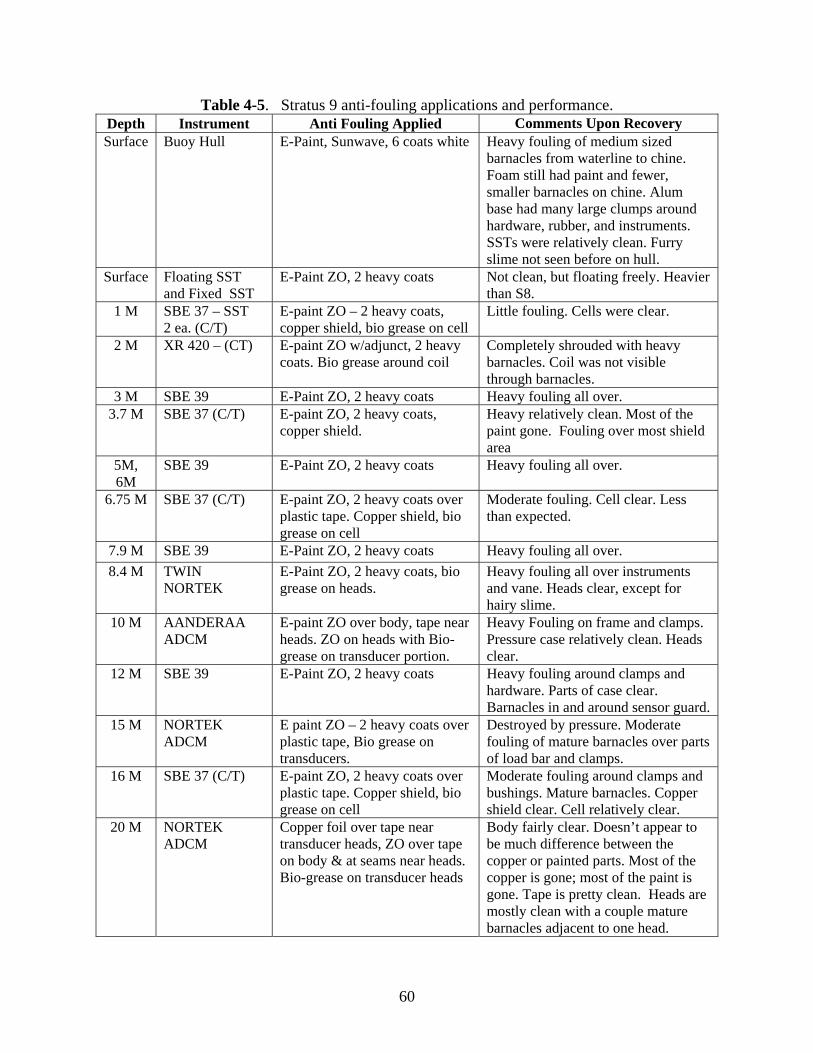
60

Table 4-5. Stratus 9 anti-fouling applications and performance. Depth Instrument Anti Fouling Applied Comments Upon Recovery Surface Buoy Hull E-Paint, Sunwave, 6 coats white Heavy fouling of medium sized

barnacles from waterline to chine. Foam still had paint and fewer, smaller barnacles on chine. Alum base had many large clumps around hardware, rubber, and instruments. SSTs were relatively clean. Furry slime not seen before on hull.

Surface Floating SST and Fixed SST

E-Paint ZO, 2 heavy coats Not clean, but floating freely. Heavier than S8.

1 M SBE 37 – SST 2 ea. (C/T)

E-paint ZO – 2 heavy coats, copper shield, bio grease on cell

Little fouling. Cells were clear.

2 M XR 420 – (CT) E-paint ZO w/adjunct, 2 heavy coats. Bio grease around coil

Completely shrouded with heavy barnacles. Coil was not visible through barnacles.

3 M SBE 39 E-Paint ZO, 2 heavy coats Heavy fouling all over. 3.7 M SBE 37 (C/T) E-paint ZO, 2 heavy coats,

copper shield. Heavy relatively clean. Most of the paint gone. Fouling over most shield area

5M, 6M

SBE 39 E-Paint ZO, 2 heavy coats Heavy fouling all over.

6.75 M SBE 37 (C/T) E-paint ZO, 2 heavy coats over plastic tape. Copper shield, bio grease on cell

Moderate fouling. Cell clear. Less than expected.

7.9 M SBE 39 E-Paint ZO, 2 heavy coats Heavy fouling all over.

8.4 M TWIN NORTEK

E-Paint ZO, 2 heavy coats, bio grease on heads.

Heavy fouling all over instruments and vane. Heads clear, except for hairy slime.

10 M AANDERAA ADCM

E-paint ZO over body, tape near heads. ZO on heads with Bio-grease on transducer portion.

Heavy Fouling on frame and clamps. Pressure case relatively clean. Heads clear.

12 M SBE 39 E-Paint ZO, 2 heavy coats Heavy fouling around clamps and hardware. Parts of case clear. Barnacles in and around sensor guard.

15 M NORTEK ADCM

E paint ZO – 2 heavy coats over plastic tape, Bio grease on transducers.

Destroyed by pressure. Moderate fouling of mature barnacles over parts of load bar and clamps.

16 M SBE 37 (C/T) E-paint ZO, 2 heavy coats over plastic tape. Copper shield, bio grease on cell

Moderate fouling around clamps and bushings. Mature barnacles. Copper shield clear. Cell relatively clear.

20 M NORTEK ADCM

Copper foil over tape near transducer heads, ZO over tape on body & at seams near heads. Bio-grease on transducer heads

Body fairly clear. Doesn’t appear to be much difference between the copper or painted parts. Most of the copper is gone; most of the paint is gone. Tape is pretty clean. Heads are mostly clean with a couple mature barnacles adjacent to one head.

61

25 M SBE 39 (Temp) E-paint ZO, 2 heavy coats Body pretty clean. Mature barnacles on load bar around clamps and bushings.

27.5 M TWIN NORTEK

E-Paint ZO, 2 heavy coats, bio grease on heads.

Instruments destroyed by pressure. Cases pretty clean. Heavy fouling on vanes. Light fouling on bars and aluminum clamps.

30 M SBE 37 (C/T) E-paint ZO, 2 heavy coats over plastic tape. Copper shield, bio grease on cell

Very few barnacles on body. Cells clear. Few mature barnacles on load bar and clamps.

32.5 M AANDERAA ADCM

E-paint ZO over body, tape near heads. ZO on heads with Bio-grease on transducer portion.

Much cleaner than 10 m unit. Heads completely clear. Few barnacles on case. Mostly on cage, clamps and bushings.

35 M SBE 39 (Temp) E-paint ZO, 2 heavy coats Body pretty clean. Few mature barnacles on load bar around clamps and bushings.

37.5 M SBE 37 (C/T) E-paint ZO, 2 heavy coats over plastic tape. Copper shield, bio grease on cell

Very few barnacles on body. Cells clear. Few mature barnacles on load bar and clamps.

40 M SBE 37 (C/T) E-paint ZO, 2 heavy coats over plastic tape. Copper shield, bio grease on cell

Very few barnacles on body. Cells clear. Few mature barnacles on load bar and clamps.

45 M VMCM ZO on propellers and sting Pretty clean. Slime and a couple barnacles on props. Body and clamps had mature barnacles.

47.5 M TWIN NORTEK

E-Paint ZO, 2 heavy coats, bio grease on heads.

Instruments destroyed by pressure. Cases pretty clean. Light fouling on vanes. Very little fouling on bars and aluminum clamps. Mostly brown slime.

50 M AANDERAA Sea Guard ADCM

E-paint ZO over body, tape near heads. ZO on heads with Bio-grease on transducer portion.

Destroyed by pressure. Much cleaner than 10 m unit. Very few, but mature barnacles on cage and clamps.

55 M VMCM ZO on propellers and sting Pretty clean. Slime and a couple barnacles on props. Body and clamps had mature barnacles. Really no difference from 45 M

62 M SBE 37 (C/T) E-paint ZO, 2 heavy coats over plastic tape. Copper shield,

Pretty clean. Some paint left. Mostly just slime over paint. A couple barnacles.

66.7 TWIN NORTEK

E-Paint ZO, 2 heavy coats, bio grease on heads.

Instruments destroyed by pressure. Cases pretty clean. Light fouling on vanes. Very little fouling on bars and aluminum clamps. Mostly brown slime.

70 SBE 39 (Temp) None Destroyed by pressure. Some slime and a couple immature barnacles.

62

V. Ancillary Projects

A. Underway Conductivity Temperature Depth (UCTD)

1) Operation

The UCTD is an underway system for acquiring conductivity and temperature profiles at ship speed up to and exceeding 13 knots. It is manufactured, packaged, and sold by Oceanscience in Oceanside, California. Our experience during the Stratus cruise was that a maximum ship speed of 11 to 11.5 knots was preferable to attain a depth between 250 and 300m, using a 500 lbs line.

The system was operated from the after portion of the stern deck. A length of line equal to the desired cast depth was wound onto the CTD's tail spool. While the ship steamed away from the drop site, the probe plunged vertically with a nearly constant drop rate independent of the ship’s speed.

Line was spooled automatically off the probe’s tail while it dropped through the water and line was manually payed out from the winch spool. The simultaneous payout of line from the probe’s tail and winch effectively made the line horizontal velocity through water zero, allowing freefall.

The CTD probe sampled conductivity, temperature, and depth at a sampling rate of 16 Hz while descending vertically through the water column at ~4 meters per second. Data was stored internally in flash memory and downloaded wirelessly via Bluetooth to a host computer or PDA after recovery. Figure 5-1 shows the UCTD winch installed on the fantail of the NOAA Ship Ronald H. Brown.

The latitude and longitude of individual casts was obtained by matching an internal time stamp in the data file header to an externally collected GPS file. Synchronization of instrument and GPS time was important. MATLAB scripts were used for processing.

Figure 5-1: UCTD Assembled.

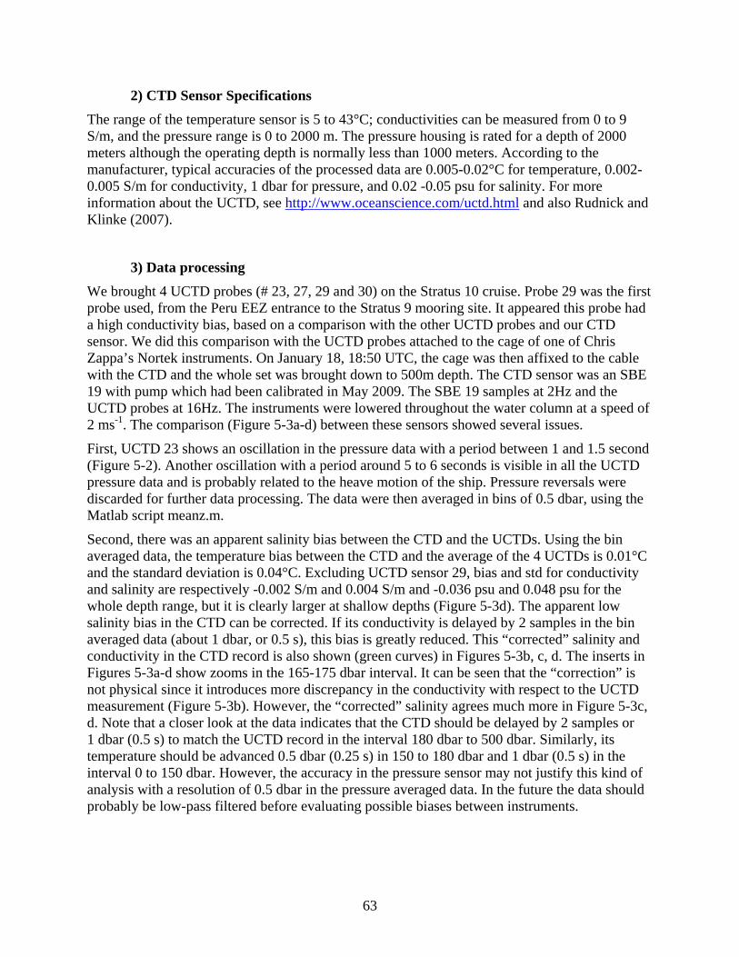
63

2) CTD Sensor Specifications

The range of the temperature sensor is 5 to 43°C; conductivities can be measured from 0 to 9 S/m, and the pressure range is 0 to 2000 m. The pressure housing is rated for a depth of 2000 meters although the operating depth is normally less than 1000 meters. According to the manufacturer, typical accuracies of the processed data are 0.005-0.02°C for temperature, 0.002-0.005 S/m for conductivity, 1 dbar for pressure, and 0.02 -0.05 psu for salinity. For more information about the UCTD, see http://www.oceanscience.com/uctd.html and also Rudnick and Klinke (2007).

3) Data processing

We brought 4 UCTD probes (# 23, 27, 29 and 30) on the Stratus 10 cruise. Probe 29 was the first probe used, from the Peru EEZ entrance to the Stratus 9 mooring site. It appeared this probe had a high conductivity bias, based on a comparison with the other UCTD probes and our CTD sensor. We did this comparison with the UCTD probes attached to the cage of one of Chris Zappa’s Nortek instruments. On January 18, 18:50 UTC, the cage was then affixed to the cable with the CTD and the whole set was brought down to 500m depth. The CTD sensor was an SBE 19 with pump which had been calibrated in May 2009. The SBE 19 samples at 2Hz and the UCTD probes at 16Hz. The instruments were lowered throughout the water column at a speed of 2 ms-1. The comparison (Figure 5-3a-d) between these sensors showed several issues.

First, UCTD 23 shows an oscillation in the pressure data with a period between 1 and 1.5 second (Figure 5-2). Another oscillation with a period around 5 to 6 seconds is visible in all the UCTD pressure data and is probably related to the heave motion of the ship. Pressure reversals were discarded for further data processing. The data were then averaged in bins of 0.5 dbar, using the Matlab script meanz.m.

Second, there was an apparent salinity bias between the CTD and the UCTDs. Using the bin averaged data, the temperature bias between the CTD and the average of the 4 UCTDs is 0.01°C and the standard deviation is 0.04°C. Excluding UCTD sensor 29, bias and std for conductivity and salinity are respectively -0.002 S/m and 0.004 S/m and -0.036 psu and 0.048 psu for the whole depth range, but it is clearly larger at shallow depths (Figure 5-3d). The apparent low salinity bias in the CTD can be corrected. If its conductivity is delayed by 2 samples in the bin averaged data (about 1 dbar, or 0.5 s), this bias is greatly reduced. This “corrected” salinity and conductivity in the CTD record is also shown (green curves) in Figures 5-3b, c, d. The inserts in Figures 5-3a-d show zooms in the 165-175 dbar interval. It can be seen that the “correction” is not physical since it introduces more discrepancy in the conductivity with respect to the UCTD measurement (Figure 5-3b). However, the “corrected” salinity agrees much more in Figure 5-3c, d. Note that a closer look at the data indicates that the CTD should be delayed by 2 samples or 1 dbar (0.5 s) to match the UCTD record in the interval 180 dbar to 500 dbar. Similarly, its temperature should be advanced 0.5 dbar (0.25 s) in 150 to 180 dbar and 1 dbar (0.5 s) in the interval 0 to 150 dbar. However, the accuracy in the pressure sensor may not justify this kind of analysis with a resolution of 0.5 dbar in the pressure averaged data. In the future the data should probably be low-pass filtered before evaluating possible biases between instruments.

64

Third, the conductivity bias between sensor 29 and average of the 3 other UCTDs is 0.036 S/m (0.039 S/m with respect to CTD). In terms of salinity this induces a bias of 0.33 psu (0.37 psu). The bias in conductivity is responsible for most of the salinity discrepancy. The conductivity bias varied from 0.0409 to 0.0479 S/m between 100 dbar and the surface. For depths > 300 dbar, the bias was under 0.0300 S/m. This may be a dependence on temperature. This results in a high bias in salinity of about 0.25 to 0.4 psu. Another test was made with all these instruments in a bucket of seawater on deck. The bucket was left undisturbed for 10 to 15 minutes (another attempt with stirring produced too much noise in the collected data). The salinity bias in UCTD#29 was also observed when two UCTD casts were done near a CTD station (Figure 5-4). All these tests point to the high conductivity bias in UCTD#29.

Another issue with the UCTD measurements is the tendency for spikes in salinity, caused by the different response time in the conductivity and temperature sensor. Using the AlignCTD option in the Seaterm software provided by Seabird, we advanced the temperature record by 0.09s with respect to conductivity which greatly reduced the salinity spikes. The advance time mentioned above works well for the UCTD probes with a fall rate of ~ 4ms-1, but this would have to be changed for a different fall rate. Note that you can align multiple files at once.

Figure 5-2. Pressure time series during CTD/UCTD comparison. Time vectors from instruments were synchronized visually and probably explain the apparent pressure biases between sensors.

65

Figure 5-3. CTD/UCTD comparison. Based on 0.5 db bin averaged data. Inserts are zooms on 165 to 175 dbar interval.

a. Pressure vs temperature. b. Pressure vs conductivity.

c. Pressure vs salinity. d. Temperature vs salinity.

66

Figure 5-4. Two UCTDs done just before and after CTD cast. T-S plot: all CTD cast (upper) and shallow part of cast (lower).

67

4) UCTD Results

All UCTD profiles were interpolated and gridded using Matlab scripts and the resulting contour plots are shown in Figures 5-5 and 5-6. Note that salinity in these plots is not corrected for the high salinity/conductivity bias in UCTD probe #29. Periods of use of the different probes is summarized in Table 5-1.

Figure 5-5. Upper: Temperature (oC) measured by UCTD. Lower: Salinity (psu) derived from measured pressure, temperature and conductivity.

Figure 5-6. Upper: Density anomaly (kg/m3). Lower: Conductivity (S/m) measured by UCTD.

68

Table 5-1. Periods of use for the different UCTD probes used during Stratus 10 cruise.

SN Usage period 29 01.13.2010 04:55 to 01.17.2010 21:27 30 01.19.2010 02:28 to 01.24.2010 02:52

01.24.2010 13:00 to 01.29.2010 03:00 01.24.2010 03:33 to 01.24.2010 04:00* 01.24.2010 05:08*

23 01.24.2010 03:10 to 01.24.2010 12:11 (except *)

B. Vertical Microstructure Profiler (VMP)

During the STRATUS 2010 cruise, measurements of upper ocean microstructure were made with the Vertical Microstructure Profiler (VMP) from Rockland Scientific. The VMP 750 and VMP 2000 are tethered microstructure profilers for the measurement of dissipation-scale turbulence in coastal and continental shelf regions. It is equipped with state-of-art microstructure velocity probes (shear probes), high-resolution temperature sensors (thermistors), and high-accuracy CTD sensors. All sensors, mechanical components, and electronics are of the highest quality. A summary of pre and post calibrations for the VMP probes is in Appendix 8. The VMP is shown in Figure 5-7 in preparation for deployment on the fantail of the NOAA Ship Ronald H. Brown. These data give a direct estimate of turbulence and mixing as well as temperature, salinity all as a function of depth. A primary goal of these data will be to compare the estimates of turbulent kinetic energy dissipation rate from the pulse-to-pulse coherent sonars deployed from the S9 buoy. A second primary goal is to survey an eddy determined from sea surface height (SSH; from satellite altimetry). Eddies are thought to contribute to the upper ocean mixing and the evolution of the mixed layer. A third goal is to measure the mixing processes and rates associated with the Eastern South Pacific Intermediate Water (ESPIW). During the STRATUS 2010 cruise, the VMP sampling consisted of two distinct surveys outlined in Table 5-2. Both surveys are shown in Figure 5-8 in the track imposed upon the plot of ADCP currents and temperature. The first survey (“Volume survey”) was a tight 6 nautical miles square around the STRATUS 10 mooring with 8 equally spaced sampling stations. The final sampling station was not completed and no data is available. This survey was completed in the SW corner of the track in Figure 5-8 (denoted by the purple spot). The second survey (“Eddy survey”) covered an area of roughly 100 nautical miles square in the region of a persistent mesoscale eddy (Figures 5-9 and 5-10). Peter Gaube (COAS, Oregon State University) provided data of satellite altimetry, which was used to locate eddies, as seen in Figure 5-10. The first leg of VMP stations began just below the STRATUS 10 mooring survey region and ran SW to NE. The top leg ran from the NE corner due West to the NW corner with UCTDs. The final leg of VMP stations ran from the NW corner to the SE corner (red diamond). A cluster of drifters was deployed during this final leg near the center of the survey. The stations for VMP sampling made an X-pattern when the survey was completed.

69

Figure 5-7. Picture of the VMP on the fantail of the NOAA ship Ronald H. Brown prior to deployment.

Figure 5-8. Detail of the cruise track for the two VMP Surveys. Purple dot denotes the location for the 1st survey around the STRATUS 10 mooring and beginning of the 2nd survey. Red diamond denotes the end of the 2nd survey of the eddy. Arrows are current vectors near surface from ships’s ADCP, colored according to water temperature.

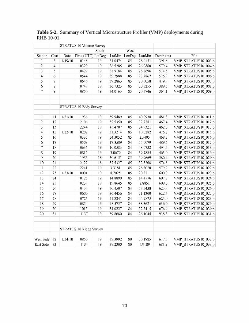
70

Table 5-2. Summary of Vertical Microstructure Profiler (VMP) deployments during RHB 10-01.

71

Figure 5-9. Location of VMP casts (blue squares) during Stratus 10 cruise and seafloor bathymetry (colored contours).

Figure 5-10. Sea surface anomaly on January 20, 2010 (colored contours) and bathymetry (black contours, contour interval 1000m).

The raw data were consolidated into *.p files. A Matlab script (“VMP_quick_look.m”) is provided to convert the raw data files into *.MAT files and to plot the relevant oceanographic data. A number of diagnostic variables are provided as well. As for the UCTD data, the GPS position of each cast was located by synchronizing the time of cast with the GPS data file from the ship. All UCTD and VMP profiles (Figure 5-11) were combined and interpolated to produce a gridded data which can be contoured as in Figure 5-12.

72

Figure 5-11. Profiles of UCTDs and VMPs during the section of the eddy survey on January 22. From top left, clockwise: conductivity, temperature, salinity and density.

73

Figure 5-12. Contour plot of UCTD and VMP profiles.

C. Ridge Survey

While heading east towards the DART buoy, two VMP profiles (600m depth) were made west and east of a seamount that is part of the Nazca ridge. A low pressure eddy was located in the area (Figure 5-10) and may have been crossing the ridge there because of a gap in the topography (Figures 5-9 and 5-13). A Seabeam survey was also done in anticipation of use in a future cruise.

Figure 5-13. Ridge survey: bathymetry (contours) from etopo2 and ship’s track survey (black line). Triangles denote the 2 VMP stations made on each side of the Nazca ridge.

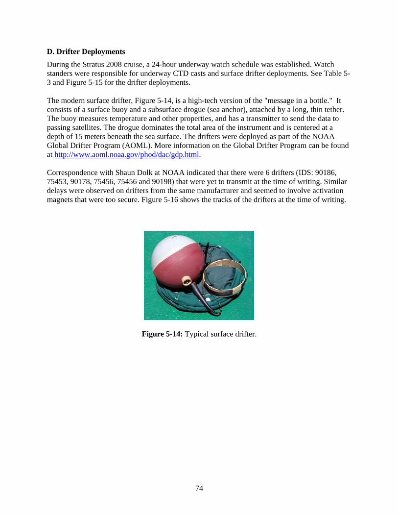
74

D. Drifter Deployments

During the Stratus 2008 cruise, a 24-hour underway watch schedule was established. Watch standers were responsible for underway CTD casts and surface drifter deployments. See Table 5-3 and Figure 5-15 for the drifter deployments.

The modern surface drifter, Figure 5-14, is a high-tech version of the "message in a bottle." It consists of a surface buoy and a subsurface drogue (sea anchor), attached by a long, thin tether. The buoy measures temperature and other properties, and has a transmitter to send the data to passing satellites. The drogue dominates the total area of the instrument and is centered at a depth of 15 meters beneath the sea surface. The drifters were deployed as part of the NOAA Global Drifter Program (AOML). More information on the Global Drifter Program can be found at http://www.aoml.noaa.gov/phod/dac/gdp.html.

Correspondence with Shaun Dolk at NOAA indicated that there were 6 drifters (IDS: 90186, 75453, 90178, 75456, 75456 and 90198) that were yet to transmit at the time of writing. Similar delays were observed on drifters from the same manufacturer and seemed to involve activation magnets that were too secure. Figure 5-16 shows the tracks of the drifters at the time of writing.

Figure 5-14: Typical surface drifter.

75

Figure 5-15. Map of drifters deployments during stratus 10 cruise (green squares). Stratus 9 and 10 mooring locations (red squares).

76

Figure 5-16. Tracks of drifters deployed during Stratus 10 cruise, as of February 18, 2010 (courtesy of Shaun Dolk, NOAA).

77

Table 5-3. Location and time of drifter launches during Stratus 10 cruise.

Drifter # ID Day Time (UTC)

hh:mm Deploy Lat

deg mm.mm Deploy Long deg mm.mm

1 90189 1/14/2010 21:42 10 30.047 84 54.829

2 90188 1/15/2010 8:17 12 31.327 85 02.491

3 90170 1/15/2010 16:15 14 00.878 85 09.085

4 90194 1/16/2010 0:13 15 32.273 85 15.947

5 90175 1/16/2010 7:59 17 01.155 85 22.984

6 90186 1/16/2010 15:46 18 29.897 85 29.386

7 90173 1/23/2010 10:10 19 41.6 83 58

8 75453 1/23/2010 20:06 19 41 83 00

9 90171 1/24/2010 0:57 19 40.4 81 59.5

10 90197 1/24/2010 6:07 19 39.82 80 59.34

11 90174 1/24/1900 12:44 19 39.21 79 59.99

12 90179 1/24/2010 17:58 19 38.58 78 59.49

13 75455 1/24/2010 22:53 19 38.011 78 00

14 90176 1/25/2010 3:55 19 37.32 76 59.11

15 90178 1/25/2010 9:03 19 36.7 75 59.18

16 90177 1/25/2010 13:56 19 36.13 75 01

17 90185 1/16/2010 18:16 18 58.031 85 31.781

18 90187 1/16/2010 19:46 19 14.744 85 33.005

19 75456 1/23/2010 0:54 19 11.72 85 17.18

20 90172 1/23/2010 3:44 19 25.5 85 02

21 90198 1/23/2010 6:43 19 38 85 49.5

22 75454 1/26/2010 11:08 21 30.51 74 21

23 75457 1/27/2010 3:50 23 30.24 73 53.510

24 90195 1/27/2010 19:57 25 29.4 73 25.97

25 90196 1/28/2010 12:20 27 30.0 72 58.037

78

E. CTD casts Two deep CTD casts (4000m) were made during this cruise, at the locations of the Stratus 9 and 10 moorings. Another one was made at the DART location (1000m). Two other casts were made for testing acoustic releases and comparing with UCTD probes. All CTD casts are shown in Figures 5-17 and summarized in Table 5-4. The CTD sensor used was a SBE19 (SN 2361) with pump, calibrated in May 2009. The CTD cable was lowered through the winch on the starboard side of the ship at a rate of 2 ms-1. The setup for the SBE 19 is shown below as issued by the command DS in the Seasoft program from Seabird: * SEACAT PROFILER V3.1 SN 2361 01/14/10 12:42:21.505 * strain gauge pressure sensor: SN = 178340, range = 10000 psia, tc = -996 * clk = 32768.070 iop = 144 vmain = 8.0 vlith = 5.8 * mode = PROFILE ncasts = 4 * sample rate = 1 scan every 0.5 seconds * minimum raw conductivity frequency for pump turn on = 3221 hertz * pump delay = 45 seconds * samples = 10879 free = 163249 lwait = 0 msec * SW1 = C0 battery cutoff = 5.8 volts * number of voltages sampled = 0 * logdata = NO

Table 5-4. CTD casts locations, times and depths during Stratus 10 cruise.

CTD #

Date Time In

Time Out

Depth (m)

lat Lon notes

1 1/14/2010 11:23 12:39 1500 -8.83846 -84.76963 with releases stop at 200m 2 1/18/2010 14:00 16:30 4000 -19.57596 -85.33055 3 1/18/2010 18:50 19:35 500 -19.59153 -85.36848 test with 4 UCTD probes 4 1/18/2010 21:59 50 test with Zappa's Nortek 5 1/19/2010 17:37 4000 -19.6643 -85.61765 6 1/25/2010 18:00 1000 DART location

Postcalibration from Seabird on SBE19 SN2361, made on 2010/04/28, indicates proper operating of this instrument (drifts since last calibration: -0.0001 PSU/month and 0.00076°C/yr for conductivity and temperature, respectively).

79

Figure 5-17. CTD casts made during Stratus 10 cruise, in chronological order from top to bottom.

80

Fig 5-17 (continued)

81

Fig 5-17 (continued)

F. Atmospheric Observations

1) Weather

During the Stratus 10 cruise, the weather conditions experienced near the buoy site were typical of the marine stratocumulus area under which the buoy is located. Relative humidity varied around 65-85%, and winds were steady from the SE usually ranging from 5-10 m/s. The air temperature was nearly constant around 20°C while SST was nearly constant around 20.5°C. Normally the atmospheric temperature is slightly cooler than SST, however these values are slightly below typical January temperatures by about 0.5-1°C. The weather for this region is fairly constant as it is dominated by the semi-permanent subtropical high. The flow around the high produces steady winds from the southeast, also known as the trade winds, which rarely reach a speed above 10 m/s. Subsidence along with cooler SSTs are associated with the high which forms stable atmospheric conditions necessary for the formation and maintenance of low level marine stratocumulus cloud decks that typically blanket the area. Consequently, this

82

general weather pattern allows for very few convective systems to affect the area. Occasionally, some mid and upper level clouds were present during the cruise near the stratocumulus region, but these were mostly advected from the Peruvian Andes and covered relatively little area. Very little rainfall is reported for this area even though these clouds frequently drizzle, especially at night when they are driven by radiative cooling. Often times, the drizzle will evaporate before it reaches the surface, altering the boundary layer conditions yet recording little to no measurements in rain gauges. For example, on the mornings of January 17 and 19, observations from the crew noticed some drizzle, even consistent rain on the 19th, yet the rain sensors on the ship recorded no or little precipitation.

2) WHOI turbulent flux sensor

The WHOI Direct Covariance Flux System (DCFS) consists of a Gill three-axis sonic anemometer-thermometer R3A-100 and a Systron Donner MotionPAK. The sonic anemometer records the three components of wind velocity used to derive direct estimates of the wind vector stress (τ) using the eddy correlation technique. The MotionPAK, attached below the sonic anemometer, contains three-axis linear accelerometers and rotational rate sensors which measure the stabilized pitch, roll and yaw and are used to help correct for the effects of platform motion. The DCFS was mounted on the fore bow mast of the Ron Brown (see Figure 5-18) at a height of 11.4 m above the mean sea surface (O1 deck is 5.6 m above waterline and sensor is 5.8 m above O1 deck, on jackstaff). Since no relative humidity sensor was available only the momentum stress can be derived from the system. The data from this sensor is processed after the cruise and includes platform motion corrections.

3) Earth system Research Laboratory (ESRL) Observations

The Physical Sciences Division (PSD) of the Earth System Research Laboratory (ESRL) ran its turbulent flux system in support of the overall meteorological part of the Stratus 10 cruise. The PSD Turbulent flux system consists of four components. A fast turbulence system with ship motion corrections mounted on the jack staff, which includes an ultrasonic anemometer, Gill Wind Master model R3A, and a Systron Donner Inertia Motion-pak unit with serial number 0681. Solar and IR radiation sensors are radiometers from The Eppley Lab, two pyranometers and two pyrgeometers mounted in a high and unobstructed sky-see location on the O2 deck. The bulk meteorology sensors are a Vaisala T/RH sensor in aspirator, a skin surface semperature (SST) made with a floating (YSI 46040) thermistor deployed off port side with outrigger, and an Optical Scientific Inc.-Optical Precipitation Sensor model ORG-815 DA. Finally, a fast sampling humidity sensor, Li-COR 7500 fast CO2/H2Ogas analyzer is mounted on the top of bow tower.

83

Figure 5-18. Turbulence Flux system setup on the jack staff of the NOAA Ship Ronald H. Brown. WHOI turbulent anemometer is at lowest level.

All the data files are in ASCII text format. The description of the data format for each data file is covered in the attached document “NOAA/PSD Ship-based Primary Turbulent Flux Data Acquisition System.”

In conjunction with the flux system PSD ran a Vaisala CL31 ceilometer for the measurement of cloud base altitude. The first processing of the raw data from the ceilometer produces 2 plots for each day. One of the plots is of the laser backscatter intensity, and the other plot is the cloud base altitude determined from the backscatter. The Vaisala output format is read by a Matlab code named “read_daily_rawceilo_CL31_STRATUS_2009.m.”

Other data collected by PSD are a series of satellite image from various meteorological or environmental satellites. The system to collect these images is called TeraScan made by the Sea Space Corporation. They are used in the final analysis of the flux data.

Raw data from the ship (SCS) and ESRL are shown in Figures 5-19. Figure 5-20 shows the ceilometer data for January 17-18 when the ship was stationed near the newly deployed Stratus 10 buoy. A Terascan image is in Figure 5-21 for January 26. Note that most Terascan pictures have very little information because of the persistent clouds in the region. The one shown here has unusually little clouds.

84

Figure 5-19. Meteorological data collected by ship system (SCS) and ESRL.

85

Figure 5-19 (continued).

86

Figure 5-20. Cloud backscatter from ESRL’s ceilometer (upper) and inferred cloud base (lower) on January 17 and 18, 2010, during Stratus 10 cruise.

87

Figure 5-21. Terrascan: Infrared imagery from NOAA satellite 17, on January 26, 2010.

G. DART

1) Overview

The Hydrographic and Oceanographic Service of the Chilean Navy (SHOA) made an effort to acquire and deploy a DART II system (Deep-Ocean Assessment and Reporting of Tsunami) for its early tsunami detection and real-time reporting capability. Although seismic networks and coastal tide gauges are indispensable for assessing the hazard during an actual event, an improvement in the speed and accuracy of real-time forecasts of tsunami inundation for specific sites requires direct tsunami measurement between the source and a threatened community. Currently, only a network of real-time reporting, deep-ocean bottom pressure (BPR) stations can provide this capability.

The DART mooring system is illustrated in Figure 5-22. Each system consists of a seafloor BPR and a moored surface buoy with related electronics for real-time communications. The BPR uses a pressure transducer manufactured by Paroscientific, Inc., to make 15-second averaged measurements of the pressure exerted on it by the overlying water column. These transducers use a very thin quartz crystal beam, electrically induced to vibrate at their lowest resonant mode. In DART II applications, the transducer is sensitive to changes in wave height of less than a millimeter. An acoustic link is used to transmit data from the BPR on the seafloor to the surface

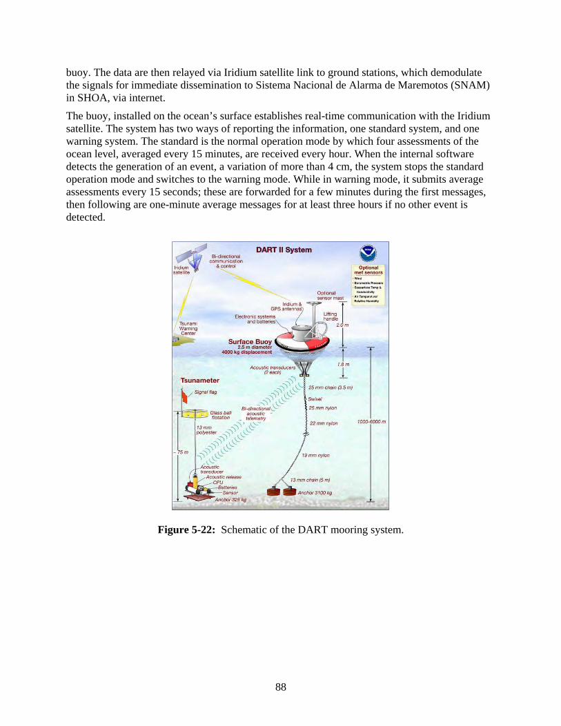
88

buoy. The data are then relayed via Iridium satellite link to ground stations, which demodulate the signals for immediate dissemination to Sistema Nacional de Alarma de Maremotos (SNAM) in SHOA, via internet.

The buoy, installed on the ocean’s surface establishes real-time communication with the Iridium satellite. The system has two ways of reporting the information, one standard system, and one warning system. The standard is the normal operation mode by which four assessments of the ocean level, averaged every 15 minutes, are received every hour. When the internal software detects the generation of an event, a variation of more than 4 cm, the system stops the standard operation mode and switches to the warning mode. While in warning mode, it submits average assessments every 15 seconds; these are forwarded for a few minutes during the first messages, then following are one-minute average messages for at least three hours if no other event is detected.

Figure 5-22: Schematic of the DART mooring system.

89

Figure 5-23: DART II surface mooring with a complete set of IMET sensors.

2) BPR Recovery

The intent on this cruise had been to go to the DART site and recover the meteorological sensors on the surface buoy (Figure 5-23), then replace them with recently calibrated meteorological sensors. This would continue the sampling of meteorology and upper ocean temperature and salinity that had begun in 2006. The DART surface mooring is recovered and redeployed on Stratus cruises every other year. The bottom pressure recorder (BPR) of the DART installation is recovered and redeployed every four years (last deployment in 2006). The DART surface mooring had last been recovered and redeployed in October 2008 and carried WHOI temperature and salinity sensors on the mooring line. While the ocean instruments were set up to sample for two years, the meteorological instruments, self-contained IMET modules and LASCAR humidity/temperature sensors were set up to sample more rapidly to match the sampling rate at the Stratus ORS. With this rapid sampling, they have to be replaced each year. During the Stratus cruise 2008, the SHOA people in accordance with WHOI scientists, replaced the batteries, mooring and anchor as well as subsurface instruments. The work was carried out between October 31 and November 1, 2008.

As this cruise began, we learned that the DART surface mooring was adrift following a break in the mooring line. As a result of the break most of the oceanographic instruments were lost. What equipment was recovered by the Chilean Navy when they found the surface buoy is summarized in Tables 5-5 and 5-6. Note that they protected the domes of the radiation sensors.

90

The Chilean Navy did ask that we recover the oceanic BPR. We went to the DART site, released and disabled the WHOI acoustic release on the sea floor at the base of the failed surface mooring (no buoyancy on this mooring), and then released the BPR acoustic release. The BPR surfaced in about 2 hours and was recovered.

Table 5-5: Status of DART surface instruments (deployed in 2008).

SURFACE INSTRUMENTATION

Post-Recovery Time

Check

MODULE Serial FIRMWARE STATUS UTC Internal HRH 505 VOSHRH53 v3.2 Good 3/23/10 13:40 13:53:13

WND 228 VOSWND53 v3.5 Good 3/23/10 15:04 15:17:00

PRC 503 VOSPRC53 v3.4 Good 3/23/10 15:44 15:53:20

LWR 206 VOSLWR53 v3.5 Good 3/23/10 14:43 14:49:03

SWR 216 VOSSWR53 v3.3 Good 3/23/10 13:55 14:04:02

BPR 201 VOSBPR53 v3.3 FLOODED

LASCAR 5 Pending 3024kb

Table 5-6: Status of DART subsurface instruments (deployed in 2008). SUBSURFACE INSTRUMENTATION

Instrument Serial Depth Status Time check UTC

Time check Internal

SBE39 44 Bridle Good data,

93774 records 3/23/10 13:40 3/23/10 17:08

SBE39 46 30m Lost

SBE39 47 40m Lost

SBE39 282 62.5m Lost

SBE39 1503 77.5m Lost

SBE39 1504 115m Lost

SBE39 1505 175m Lost

SBE39 1506 220m Lost

SBE39 1508 250m Lost

SBE39 1510 310m Lost

XR420 10514 145 Lost

XR420 15214 10 FLOODED, cell damaged

XR420 15215 20 Lost

XR420 15216 50 Lost

XR420 15217 92.5 Lost

Release 8242

33038 4943 Lost

91

H. ADCP

Currents were measured using the Acoustic Doppler Current Profiler (ADCP) mounted on the hull of the NOAA Ship Ronald H. Brown. This ADCP is a RDI Ocean Surveyor that operates at 75 kHz (OS75). It can be used in a narrow or broadband mode (nb75 and bb75 respectively). The resolution of nb75 is 16 m which corresponds to the bin size and there are 70 bins (8m and 75 bins for bb75). The transducer’s depth is 5m and the blanking distance is 8m for both modes so that the shallowest bin is 29m for nb75 and 21m for bb75.

Figure 5-24 below shows an example of the velocity profile during the southward transit between the Peru EEZ (dashed black lines) and the location of Stratus 10 deployment. The broadband had a better resolution but would sometimes miss data (white regions), which the narrowband did not seem to have (not shown).

Figure 5-24. Current (m/s) eastward and northward from ADCP broadband.

92

I. Student Note (Jessica Ram)

As a graduate student in atmospheric science studying marine stratocumulus, participating in the Stratus 10 cruise was an amazing opportunity. My master’s thesis focuses on satellite observations of marine stratocumulus in three subtropical regions, one of them being the region off of the South American coast. The main focus for the cruise was to recover and deploy a buoy that takes in-situ measurements for this stratocumulus region. Until this experience all of my work has been done sitting at a desk in front of a computer, and this cruise was an opportunity to experience in person the phenomena that I study.

An added benefit to being on the cruise was that while we were in the buoy region, the satellite that I am using for my research, CloudSat, passed by very close to the ship. On January 18th CloudSat came within 5.51 km and on the 20th it was within 10.69 km. At these times I took pictures and recorded observations. I look forward to comparing my observations and the ships data with the satellite products for these passes. In-situ observations and verifications for satellite data are almost non-existent for this region, so this is undoubtedly exciting information to have.

One of the first things I learned on the cruise was how much I did not know about oceanography, even though the ocean-atmosphere interactions play a huge role in atmospheric science. That being said, I certainly learned a lot as well. As an atmospheric scientist, I first think of SST when it comes to the ocean. The first week on the cruise there was a science team meeting that explained the importance of the many processes under the ocean surface that have an equally important influence over oceanic and atmospheric dynamics.

After we entered the Peruvian EEZ, we began casting UCTDs. This was my first experience with an oceanographic instrument. Learning to cast a UCTD was interesting because of the complications of taking measurements from the ocean. I thought it was clever how the instrument was spooled so that the CTD would drop straight down while the boat was still moving. When I first saw the plots that came from a CTD cast, they immediately reminded me of an atmospheric sounding, only for the ocean. The wealth of knowledge that can come from just one of these plots is incredibly useful.

When the ship was stopped near the buoy sites, we were able to use other instruments such as the deep CTD, which was a more thorough version of the UCTD, and the VMP. The VMP, or vertical microstructure profiler, is equipped with prong like sensors that measure turbulence among other things beneath the surface. The deep CTDs and the VMP data were taken intermittently around the buoy sites when the ship was not moving. There were also drifters, which were packaged instruments that we threw overboard at certain predetermined coordinates. The drifters help to track surface currents over the timescale of years for locations that scientists rarely have in-situ measurements for. All of these instruments above were new to me before this cruise.

When it came time to retrieve the old buoy and deploy the new buoy, I was impressed by the efficiency of how these processes were done. The acoustic release to find the buoy line and the cranes and winches used to maneuver things in and out of the water were proof of how well thought out and planned everything was. I can see why it is essential to have a research vessel of this size that is so well equipped. After recovering the Stratus 9 buoy, it became apparent why it is necessary to plan this cruise on an annual basis. The condition of the instruments themselves needs to be checked as well as making sure that the data is always calibrated correctly. Of course for this particular cruise, some of the instruments did not make it due to a break in one of the

93

instrument cages causing the mooring line to split. This sent some instruments to depths and pressures much further than they were designed for, destroying some of the data. This was certainly an interesting twist to the recovery, as I’m sure it doesn’t happen very often. There are still more questions to be answered about why this would happen.

In between the two sites, we spent one day close to the new buoy and one day close to the old buoy. This was so that the ship’s data could later be compared to the data from each buoy for about a 24 hour period and used in calibrations. This was especially neat to be around because every instrument used in the scientific community needs to be calibrated, but usually this process is taken for granted and assumed to have taken place.

Overall this research cruise has been an eye-opening experience for me in terms of what it takes to maintain in-situ data. Over land I’ve seen that the process can also be difficult, but with its own set of complications. It appears that in order to study oceanographic science, one needs to know equally as much about topics not directly related to oceanographic science so that they can produce useful and accurate measurements. Learning about the antifoulants and special paints to protect against ocean conditions and marine life are just part of the process to obtain these measurements. Also, the design of the instruments and the tools used to put them in place were another set of concerns that needed to be thought of.

While the importance of the data coming from these buoys and cruises cannot be overstated, this cruise was also a reminder to me of how important remote sensing is for isolated regions such as this. This single buoy provides data that represents a large area in a location that we would otherwise have no other surface observations for. Another amazing feat about the buoy is the amount of time it has been around, providing years of data. Combining the in-situ data for this area with satellite observations can only enhance our understanding of the processes being studied.

One of the last things I’ve gained from this experience was meeting the other scientists on board. On this trip I met Bob Weller and other WHOI scientists, as well as Chris Zappa from the Lamont-Doherty Earth Observatory and Bill Otto from the Earth System Research Laboratory. Everyone was extremely accommodating and very patient in helping explain everything to me. The connections I’ve made with these people could certainly serve as useful resources for the future.

I am extremely thankful for all that I have experienced during the Stratus 10 cruise. Not only was it a unique opportunity to travel to the remote location that I am researching, but I also leave this trip with abundantly more knowledge, and data, than I came with. Every scientist should have an opportunity such as this to experience what it takes in order to collect the data they use.

94

Thanks and Acknowledgements We wish to thank the officers and crew of the NOAA Ship Ronald H. Brown for their great work, especially during the difficult recovery of the Stratus 9 mooring, and for making us feel welcome onboard. A special thank you goes to Bruce Cowden and the deck crew and to Jonathan Shannahof for his help with the ship scientific equipment and his participation, early in the morning, in the ridge survey. Personnel on the bridge were very helpful and we appreciate all the time they spent to understand our work and accommodate our projects. We also thank Peter Gaube and Dudley Chelton for providing sea surface anomaly data. All contributors to this report as well as Fernando Mingram (SHOA) and Ben Pietro (WHOI) are greatly acknowledged, especially for their dedication during UCTD watches. References Colbo K. and Weller R. A., 2009. Accuracy of the IMET Sensor Package in the Subtropics.

Journal of Atmospheric and Oceanic Technology, vol. 26, pp 1867-1890. Rudnick D. L. and Klinke J., 2007. The underway Conductivity-Temperature-Depth instrument.

Journal of Atmospheric and Oceanic Technology, vol. 24, pp 1910-1923. Serra Y. L. and A’Hearn P., Freitag H. P., McPhaden M. J., 2001. ATLAS self-siphoning rain

gauge error estimates. Journal of Atmospheric and Oceanic Technology, vol.18, pp 1989-2002.

95

APPENDIX 1: Buoy Spins

Stratus 10 Buoy Spin Charleston, SC

73 Heading

Time Date Vanes Secured UTC 14:12:00 31-Dec-09

System 1 Vane Compass Direction Sample Time Logger L-01 Stop Sampling 14:50:00 SWND 210 30.80 207.30 14:51:00Restart Sampling 14:51:00 SL WND343 351.80 83.90 75.70 14:55:00

System 2 Vane Compass Direction Sample Time Logger L-02 Stop Sampling 14:52:00 WND348 354.10 781.10 72.20 14:53:00Restart Sampling 14:55:00

96

Stratus 10 Buoy Spin Charleston, SC

73 Heading

Time Date Vanes Secured UTC 15:03:00 31-Dec-09

System 1 Vane Compass Direction Sample Time Logger L-01 Stop Sampling 15:18:00 SWND 210 346.20 250.80 15:19:00Restart Sampling 15:20:00 SL WND343 308.60 125.90 74.50 15:22:00

System 2 Vane Compass Direction Sample Time Logger L-02 Stop Sampling 15:20:00 WND348 310.50 120.10 70.60 15:21:00Restart Sampling 15:22:00

97

Stratus 10 Buoy Spin Charleston, SC

73 Heading

Time Date Vanes Secured UTC 15:28:00 31-Dec-09

System 1 Vane Compass Direction Sample Time Logger L-01 Stop Sampling 15:45:00 SWND 210 262.90 300.60 15:46:00Restart Sampling 15:47:00 SL WND343 259.80 174.20 74.00 15:51:00

System 2 Vane Compass Direction Sample Time Logger L-02 Stop Sampling 15:47:00 WND348 263.00 166.90 69.90 15:48:00Restart Sampling 15:50:00 Page 3

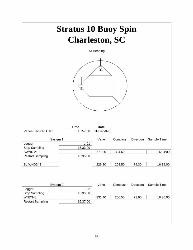
98

Stratus 10 Buoy Spin Charleston, SC

73 Heading

Time Date Vanes Secured UTC 15:57:00 31-Dec-09

System 1 Vane Compass Direction Sample Time Logger L-01 Stop Sampling 16:33:00 SWND 210 271.00 334.60 16:34:00Restart Sampling 16:35:00 SL WND343 225.80 208.50 74.30 16:39:00

System 2 Vane Compass Direction Sample Time Logger L-02 Stop Sampling 16:35:00 WND348 231.40 200.50 71.90 16:36:00Restart Sampling 16:37:00

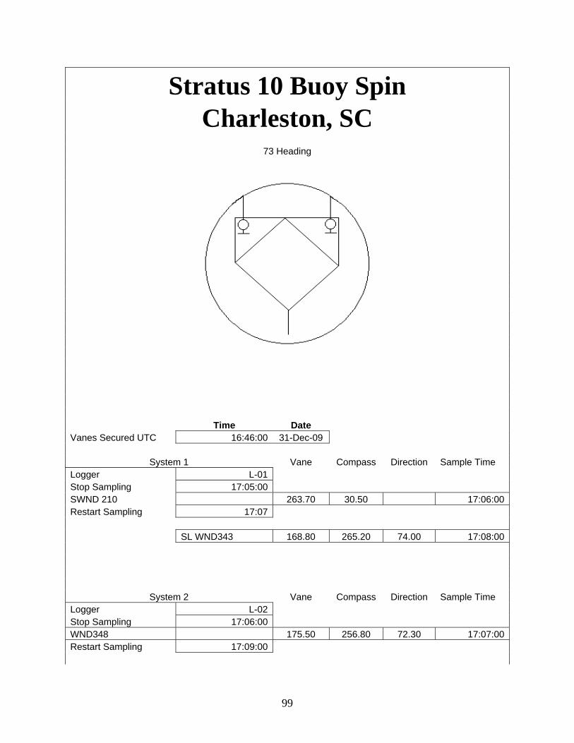
99

Stratus 10 Buoy Spin Charleston, SC

73 Heading

Time Date Vanes Secured UTC 16:46:00 31-Dec-09

System 1 Vane Compass Direction Sample Time Logger L-01 Stop Sampling 17:05:00 SWND 210 263.70 30.50 17:06:00Restart Sampling 17:07 SL WND343 168.80 265.20 74.00 17:08:00

System 2 Vane Compass Direction Sample Time Logger L-02 Stop Sampling 17:06:00 WND348 175.50 256.80 72.30 17:07:00Restart Sampling 17:09:00

100

Stratus 10 Buoy Spin Charleston, SC

73 Heading

Time Date Vanes Secured UTC 17:15:00 31-Dec-09

System 1 Vane Compass Direction Sample Time Logger L-01 Stop Sampling 17:30:00 SWND 210 175.60 76.10 17:31:00Restart Sampling 17:32:00 SL WND343 124.50 308.60 73.10 17:35:00

System 2 Vane Compass Direction Sample Time Logger L-02 Stop Sampling 17:31:00 WND348 131.90 303.00 74.90 17:32:00Restart Sampling 17:33:00

101

Stratus 10 Buoy Spin Charleston, SC

73 Heading

Time Date Vanes Secured UTC 17:42:00 31-Dec-09

System 1 Vane Compass Direction Sample Time Logger L-01 Stop Sampling 18:00:00 SWND 210 170.50 117.80 18:01:00Restart Sampling 18:02:00 SL WND343 83.60 350.60 74.20 18:04:00

System 2 Vane Compass Direction Sample Time Logger L-02 Stop Sampling 18:02:00 WND348 90.10 343.60 73.70 18:03:00Restart Sampling 18:32:00

102

Stratus 10 Buoy Spin Charleston, SC

73 Heading

Time Date Vanes Secured UTC 18:10:00 31-Dec-09

System 1 Vane Compass Direction Sample Time Logger L-01 Stop Sampling 18:30:00 SWND 210 189.80 155.80 18:31:00Restart Sampling 18:32:00 SL WND343 45.30 30.30 75.60 18:33:00

System 2 Vane Compass Direction Sample Time Logger L-02 Stop Sampling 18:35:00 WND348 49.90 24.30 74.20 18:36:00Restart Sampling 18:37:00 Page 8

103

APPENDIX 2: Subsurface Seabird Recorders Setup

SST SBE 37: SBE37-SM 485 V 2.3b SERIAL NO. 1839 05 Jan 2010 15:00:38 logging data sample interval = 300 seconds samplenumber = 169, free = 21520670 A/D cycles to average = 4 temperature = 20.72 deg C SBE37-SM 485 V 2.3b SERIAL NO. 1725 05 Jan 2010 15:01:42 logging data sample interval = 300 seconds samplenumber = 169, free = 21520670 A/D cycles to average = 4 temperature = 20.79 deg C Subsurface SBE 37s: SBE37-SM V 2.6b SERIAL NO. 1304 05 Jan 2010 13:56:44 logging data sample interval = 300 seconds samplenumber = 156, free = 232860 number of samples to average = 2 wait time after serial sync sampling = 30 seconds temperature = 20.56 deg C SBE37-SM V 1.6 SERIAL NO. 0009 05 Jan 2010 13:57:41 logging data sample interval = 300 seconds samplenumber = 156, free = 112711 A/D cycles to average = 2 wait time after serial sync sampling = 30 seconds temperature = 20.69 deg C SBE37-SM V 1.6 SERIAL NO. 0010 05 Jan 2010 13:58:46 logging data sample interval = 300 seconds samplenumber = 156, free = 115442 A/D cycles to average = 2 wait time after serial sync sampling = 120 seconds temperature = 20.45 deg C SBE37-SM V 2.6b SERIAL NO. 1912 05 Jan 2010 13:59:44 logging data sample interval = 300 seconds samplenumber = 156, free = 190494 number of samples to average = 4 wait time after serial sync sampling = 30 seconds temperature = 20.66 deg C

104

SBE37-SM V 2.6b SERIAL NO. 1907 05 Jan 2010 14:00:46 logging data sample interval = 300 seconds samplenumber = 157, free = 232859 number of samples to average = 4 wait time after serial sync sampling = 30 seconds temperature = 20.65 deg C SBE37-SM V 2.6b SERIAL NO. 1905 05 Jan 2010 14:01:39 logging data sample interval = 300 seconds samplenumber = 157, free = 232859 number of samples to average = 4 wait time after serial sync sampling = 30 seconds temperature = 20.67 deg C SBE37-SM V 2.6b SERIAL NO. 1903 05 Jan 2010 14:02:20 logging data sample interval = 300 seconds samplenumber = 157, free = 232859 number of samples to average = 4 wait time after serial sync sampling = 30 seconds temperature = 20.66 deg C SBE37-SM V 2.6b SERIAL NO. 1902 05 Jan 2010 14:03:26 logging data sample interval = 300 seconds samplenumber = 157, free = 232859 number of samples to average = 4 wait time after serial sync sampling = 30 seconds temperature = 20.73 deg C SBE37-SM V 2.6b SERIAL NO. 1910 05 Jan 2010 14:04:12 logging data sample interval = 300 seconds samplenumber = 157, free = 190493 number of samples to average = 4 wait time after serial sync sampling = 30 seconds temperature = 20.73 deg C SBE37-SM V 2.6b SERIAL NO. 2011 05 Jan 2010 14:04:51 logging data sample interval = 300 seconds samplenumber = 157, free = 232859 number of samples to average = 4 wait time after serial sync sampling = 30 seconds temperature = 20.70 deg C SBE37-SM V 2.6b SERIAL NO. 1901 05 Jan 2010 14:05:39 logging data sample interval = 300 seconds

105

samplenumber = 158, free = 232858 number of samples to average = 4 wait time after serial sync sampling = 30 seconds temperature = 20.65 deg C SBE37-SM V 2.6b SERIAL NO. 1900 05 Jan 2010 14:06:21 logging data sample interval = 300 seconds samplenumber = 158, free = 232858 number of samples to average = 4 wait time after serial sync sampling = 30 seconds temperature = 20.57 deg C SBE37-SM V 2.6b SERIAL NO. 1899 05 Jan 2010 14:07:10 logging data sample interval = 300 seconds samplenumber = 158, free = 232858 number of samples to average = 4 wait time after serial sync sampling = 30 seconds temperature = 20.50 deg C SBE37-SM V 2.6b SERIAL NO. 3639 05 Jan 2010 14:11:28 logging data sample interval = 300 seconds samplenumber = 157, free = 190493 number of samples to average = 4 wait time after serial sync sampling = 30 seconds temperature = 20.56 deg C Subsurface SBE 39s: SBE 39 V 2.0 SERIAL NO. 1502 05 Jan 2010 14:25:38 battery voltage = 9.1 logging data sample interval = 300 seconds samplenumber = 162, free = 599024 temperature = 20.80 deg C SBE 39 V 2.2 SERIAL NO. 1446 05 Jan 2010 14:26:43 battery voltage = 9.2 logging data sample interval = 300 seconds samplenumber = 162, free = 599024 temperature = 20.51 deg C SBE 39 V 3.0a SERIAL NO. 3439 05 Jan 2010 14:29:22 battery voltage = 9.2 logging data sample interval = 300 seconds samplenumber = 162, free = 599024 temperature = 21.08 deg C

106

SBE 39 V 3.0a SERIAL NO. 3435 05 Jan 2010 14:31:01 battery voltage = 9.1 logging data sample interval = 300 seconds samplenumber = 163, free = 599023 temperature = 21.52 deg C SBE 39 V 3.0a SERIAL NO. 3434 05 Jan 2010 14:32:24 battery voltage = 9.2 logging data sample interval = 300 seconds samplenumber = 163, free = 599023 temperature = 20.55 deg C SBE 39 V 3.0a SERIAL NO. 3438 05 Jan 2010 14:35:14 battery voltage = 9.1 logging data sample interval = 300 seconds samplenumber = 164, free = 599022 temperature = 20.65 deg C SBE 39 V 3.0a SERIAL NO. 3437 05 Jan 2010 14:37:45 battery voltage = 9.1 logging data sample interval = 300 seconds samplenumber = 21, free = 599165 temperature = 21.03 deg C SBE 39 V 1.7 SERIAL NO. 00203 05 Jan 2010 14:39:32 logging data sample interval = 300 seconds samplenumber = 164, free = 299429 temperature = 20.99 deg C SBE 39 V 1.7a SERIAL NO. 00721 05 Jan 2010 14:41:54 logging data sample interval = 300 seconds samplenumber = 165, free = 299428 temperature = 20.53 deg C SBE 39 V 3.0a SERIAL NO. 3423 05 Jan 2010 14:43:41 battery voltage = 9.1 logging data sample interval = 300 seconds samplenumber = 165, free = 599021 temperature = 20.88 deg C

107

APPENDIX 3: Acoustic Current Meters Setup Compass calibrations of Nortek current meters and profilers and RDI for Stratus 10

Compass Calibration for Norteks and RDI: Heading Nortek Nortek Nortek Nortek Nortek Nortek RDI

S/N: 2082 2064 1666 1688 333 357 12254 0 0.8 0.7 359.8 0.3 0.7 1.4 0.51 20 21.1 22 20.3 21.4 21.4 22.6 20.25 40 41.1 42.3 40.1 42.1 40.8 42.1 40.29 60 60.8 62.5 60.5 62.6 60.5 62.2 60.53 80 80.7 81.8 79.9 83 79.3 82.6 80.3

100 100.1 101.6 99.4 102.8 99.3 103.3 100.37 120 119.3 121.1 119 123.2 118.1 123.2 119.89 140 138.9 140 138 142.3 138.1 143.1 139.85 160 158.7 159.8 157.5 161.5 157.5 162.3 159.84 180 178.1 178.8 177.6 180.6 177.4 180.6 179.98 200 197.6 197.6 197.7 199.2 197.4 199.2 199.83 220 217.5 217 218.1 218.3 217.4 218.8 219.75 240 237.6 236.4 237.8 237.6 237.1 237 239.39 260 257.8 256.1 257.8 257.1 257.2 256.2 259.64 280 278.1 277.5 278.6 277.2 277.6 276.6 279.35 300 298.2 297.7 298.1 296.9 298.1 297.9 299.91 320 319.3 318.8 319.1 318 320.1 319.5 320.31 340 340.2 340.5 339.3 338.4 341.3 140.4 340.23

0 0.6 1 0 0.1 1 1.5 0.39

108

APPENDIX 4: VMCM Setup VM001 Model: STAR ENGINEERIN SerNum: VM2034 CfgDat: 09APR02 Firmware: VMCM2 v3.10 RTClock: 2010/01/10 19:34:15 Logging Interval: 60; Current Tick: 15 EDI Intel-compatible 20MB PCMCIA CARD present - CARD OK! FLASH card capacity: 20840436 Records used: 72; available: 612882 Main Battery Voltage: 15.13 TPOD Firmware: VMTPOD53 v3.00 TPOD Info: VMTPOD VMT034 25JUN09 THERM034 Sampling GO VM001 Model: STAR ENG. SerNum: VM2003 CfgDat: 05APR02 Firmware: VMCM2 v3.10 RTClock: 2010/01/10 19:34:37 Logging Interval: 60; Current Tick: 6 EDI Intel-compatible 20MB PCMCIA CARD present - CARD OK! FLASH card capacity: 20840436 Records used: 54; available: 612900 Main Battery Voltage: 15.19 TPOD Firmware: VMTPOD53 v3.00 TPOD Info: VMTPOD VMT013 24JUL09 THERM013 Sampling GO VM001 Model: STAR ENGINEERIN SerNum: VM2076 CfgDat: 16APR02 Firmware: VMCM2 v3.10 RTClock: 2010/01/10 19:34:56 Logging Interval: 60; Current Tick: 7 EDI Intel-compatible 20MB PCMCIA CARD present - CARD OK! FLASH card capacity: 20840436 Records used: 48; available: 612906 Main Battery Voltage: 15.12 TPOD Firmware: VMTPOD53 v3.00 TPOD Info: VMTPOD VMT033 24JUL09 THERM033 Sampling GO

109

VM001 Model: STAR ENGINEERIN SerNum: VM2014 CfgDat: 08APR02 Firmware: VMCM2 v3.10 RTClock: 2010/01/10 19:35:16 Logging Interval: 60; Current Tick: 7 EDI Intel-compatible 20MB PCMCIA CARD present - CARD OK! FLASH card capacity: 20840436 Records used: 42; available: 612912 Main Battery Voltage: 15.22 TPOD Firmware: VMTPOD53 v3.00 TPOD Info: VMTPOD VMT066 24JUL09 THERM066 Sampling GO VM001 Model: STAR ENGINEERIN SerNum: VM2037 CfgDat: 09APR02 Firmware: VMCM2 v3.10 RTClock: 2010/01/10 19:35:35 Logging Interval: 60; Current Tick: 55 EDI Intel-compatible 20MB PCMCIA CARD present - CARD OK! FLASH card capacity: 20840436 Records used: 34; available: 612920 Main Battery Voltage: 15.20 TPOD Firmware: VMTPOD53 v3.00 TPOD Info: VMTPOD VMT002 24JUL09 THERM002 Sampling GO VM001 Model: STAR ENGINEERIN SerNum: VM2040 CfgDat: 09APR02 Firmware: VMCM2 v3.10 RTClock: 2010/01/10 19:35:56 Logging Interval: 60; Current Tick: 46 EDI Intel-compatible 20MB PCMCIA CARD present - CARD OK! FLASH card capacity: 20840436 Records used: 30; available: 612924 Main Battery Voltage: 15.05 TPOD Firmware: VMTPOD53 v3.00 TPOD Info: VMTPOD VMT040 25JUN09 THERM040 Sampling GO

110

VM001 Model: STAR ENGINEERIN SerNum: VM2053 CfgDat: 15APR02 Firmware: VMCM2 v3.10 RTClock: 2010/01/10 19:36:29 Logging Interval: 60; Current Tick: 45 EDI Intel-compatible 20MB PCMCIA CARD present - CARD OK! FLASH card capacity: 20840436 Records used: 25; available: 612929 Main Battery Voltage: 14.99 TPOD Firmware: VMTPOD53 v3.00 TPOD Info: VMTPOD VMT063 24JUL09 THERM063 Sampling GO VM001 Model: STAR ENGINEERIN SerNum: VM2029 CfgDat: 09APR02 Firmware: VMCM2 v3.10 RTClock: 2010/01/10 19:37:00 Logging Interval: 60; Current Tick: 41 EDI Intel-compatible 20MB PCMCIA CARD present - CARD OK! FLASH card capacity: 20840436 Records used: 20; available: 612934 Main Battery Voltage: 15.22 TPOD Firmware: VMTPOD53 v3.00 TPOD Info: VMTPOD VMT029 25JUN09 THERM029 Sampling GO

111

APPENDIX 5: Stratus 10 Mooring Log

112

113

114

115

116

117

118

APPENDIX 6: Stratus 9 Mooring Diagram

119

120

APPENDIX 7: Stratus 9 Mooring Log

121

122

123

124

125

126

127

128

APPENDIX 8: VMP probes used in 2008/2010 Stratus cruises and available pre/post-calibration summaries. Probe Cruise Pre Cal Post Cal Notes C22 Vocals 2008 M383 Vocals 2008 09/18/2008 Error [-1.3 0.8]/1000 (pre) M382 Vocals 2008 09/18/2008 Error [-0.4 0.5]/1000 (pre) T209 Vocals 2008 T276 Vocals 2008 C22 Stratus 10,

2010

M309 Stratus 10, 2010

Error [-0.3 0.4]/1000 (pre)

M307/317 Stratus 10, 2010

M305 Stratus 10, 2010

09/19/2008 Error [-0.2 0.5]/1000 (pre)

T199 Stratus 10, 2010

T275 Stratus 10, 2010

SBE 03F SN 032874

09/16/2008 04/21/2010 drift: 0.68 mdeg/yr

SBE 04C SN 042053

09/09/2008 04/21/2010 drift: -0.5 10-3 PSU/month

SBE05T SN 054099

04/21/2010 Passed 10,000PSI test Replaced O-rings, washers

1. REPORT NO.

4. Title and Subtitle

7. Author(s)

9. Performing Organization Name and Address

12. Sponsoring Organization Name and Address

15. Supplementary Notes

16. Abstract (Limit: 200 words)

17. Document Analysis a. Descriptors

b. Identifiers/Open-Ended Terms

c. COSATI Field/Group

18. Availability Statement

REPORT DOCUMENTATIONPAGE

2. 3. Recipient's Accession No.

5. Report Date

6.

8. Performing Organization Rept. No.

10. Project/Task/Work Unit No.

11. Contract(C) or Grant(G) No.

(C)

(G)

13. Type of Report & Period Covered

14.

50272-101

19. Security Class (This Report)

20. Security Class (This Page)

21. No. of Pages

22. Price

OPTIONAL FORM 272 (4-77)(Formerly NTIS-35)Department of Commerce

(See ANSI-Z39.18) See Instructions on Reverse

UNCLASSIFIED

WHOI-2010-05

Stratus 10 Tenth Setting of the Stratus Ocean Reference Station Cruise RB-10-01

January 2 - January 30, 2010 Charleston, South Carolina - Valparaiso, Chile

May 2010

Sebastien Bigorre, Robert Weller, Jeff Lord, Nancy Galbraith, Sean Whelan,Chris Zappa, William Otto, Jessica Ram, Raul Vasquez, Diane Suhm

Woods Hole Oceanographic InstitutionWoods Hole, Massachusetts 02543

NA17RJ1223

Technical ReportNOAA/CICOR

The Ocean Reference Station at 20°S, 85°W under the stratus clouds west of northern Chile is being maintained to provide ongoing climate-quality records of surface meteorology, air-sea fluxes of heat, freshwater, and momentum, and of upper ocean temperature, salinity, and velocity variability. The Stratus Ocean Reference Station (ORS Stratus) is supported by the National Oceanic and Atmospheric Administration’s (NOAA) Climate Observation Program. It is recovered and redeployed annually, withpast cruises that have come between October and December. Due to necessary repairs on the electric motors of the ship’s propulsion system, this year the cruise was delayed until January. During the 2009/2010 cruise on the NOAA ship Ronald H. Brown to the ORS Stratus site, the primary activities were the recovery of the Stratus 9 WHOI surface mooring that had been deployed in October 2008, deployment of a new (Stratus 10) WHOI surface mooring at that site, in-situ calibration of the buoy meteorological sensors by comparison with instrumentation installed on the ship by staff of the NOAA Earth System Research Laboratory (ESRL), and collection of underway and on station oceanographic data to continue to characterize the upper ocean in the stratus region. Both underway CTD (UCTD) profiles and Vertical Microstructure Profiles (VMP) were collected along the track and during surveys dedicated to investigating eddy variability in the region. Surface drifters were also launched along the track. The intent was also to visit a buoy for the Pacific tsunami warning system maintained by the Hydrographic and Oceanographic Service of the Chilean Navy (SHOA). This DART (Deep-Ocean Assessment and Reporting of Tsunami) buoy hadbeen equipped with IMET sensors and subsurface oceanographic instruments, and a recovery and replacement of the IMET sensors was planned. However, the DART buoy broke free from its mooring on January 3rd and was recovered by the Chilean navy; the work done at that site during this cruise was the recovery of the bottom pressure unit.

Ocean Reference StationCruise ReportAir-Sea Interaction

139Approved for public release; distribution unlimited.

This report should be cited as: Woods Hole Oceanographic Institution Tech. Report, WHOI-2010-05.