455 WOODS HOLE OCEANOGRAPHIC INSTITUTION MASS · PDF fileAD-AGG82 455 WOODS HOLE OCEANOGRAPHIC INSTITUTION MASS FIG8/ ... Charles D. Hollister ... Bert University of Gothenburg

AD-AGG82 455 WOODS HOLE OCEANOGRAPHIC INSTITUTION MASS FIG8/1979 SUMMER STUDY PROGRAM IN GEOPHYSICAL FLUID DYNAMICS AT THE --ETC(U)NOV 79 M E STERN, F K MELLOR N0001-79-C-0671

UNCLASSIFIED WHOI-79-84-VOL-2 HL

. EEEEEEEEEEEEllllEllllEEEE-EEEEEEEllEEEEEEIIIIIIIEEIEEEIIIIEEEEIIEEmmhmhEEImhmh-mEEEmmhmhhmhE

007

WH01-79-844 /

19797-1 VOLUME ]I7-

......................................... ... ..................................

........... .. .............. ....... .............

...................

....... ................ ......... ..... .. .......... .. ..... ............ .......... ...... .......... ....... ...... ...... ..... ........ ..... ............. .. ...... .... .

........ ....... .......... .... X ..............

... ...... .. . ...

.. ... .. ... ...... .. ...... - T.P.".... . .....

.. .......... .... ...... ..... ..... ....................'s + WT

...... .. .... .. ...... .... ..... ....... .... .... ....... ......... ...... .. ........ ........ ...... .... .... ...... ....... ... .. ............... .... ..................................

...... .....

..... .. .. .

....... ............ ............. ....... .................. . .................................. . .................................. ............... ....................... .... ..................................................... .... ................ ............. ..... .................................. ....................... .......................... .......I .,.................... ......................... ..........I ............................. ........................................ ................1 ...................... ......................... ......... ............................ ....... ................................................ .... ..... . ......., ................ .. ..... .......... .. . .. ....... ..................................I ...............................I ........I ... ........... ........... .....................

....... ........ .................... .. ........... ......................... ... .. ..... ......... ............ ....... .............................

Me d ent nfar pt&blc czP-PrOvedcaftibutiM a and Salo; 11.3

ndted.

LECTURES of the FELLOWS

C)L- -- )

(2 1979 SUERTUDY~gROGRA4

'I

1 ~ -EOPHYSICAL JLUID DNM\THE.OODS _OLE QCEAAOGRAPHIC INSTITUTION,, .

NOTES ONPOLAR QCEANOGRAPHY - VoltS , .

L) Melvin E. Stern Directorand-

Florence K. Mellor Editor

WOODS HOLE OCEANOGRAPHIC INSTITUTION

Woods Hole, Massachusetts 02543

(::) CHNICAL P

Prepared for the Oftice of Naval Research underfGoatr 4*14-79-C7 0671 .

LReproduction in whole or in part is permitted for any purpose

of the United States Government. This report should be cited as:/Woods Hole Oceanographic Institution Technical Report WHOI-79-84'

Approved for public release; distribution unlimited.

Approved for Distribution - ,i L -Charles D. Hollister

Dean of Graduate Studies

Lii

1979 SUMMER STUDY PROGRAM

in

GEOPHYSICAL FLUID DYNAMICS

at

,. THE WOODS HOLE OCEANOGRAPHIC INSTITUTION

NOTES ON POLAR OCEANOGRAPHY

T

~Access on For

~DDC TABUAnsimounred

JuStif ication

[By__

, [ ~ ~~~Avbilt I :,Dist. a:,ior

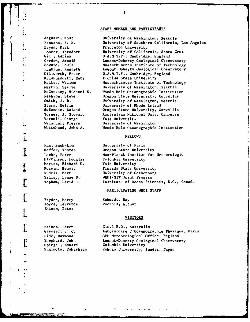
STAFF MEMBER AND PARTICIPANTS

Aagaard, Knut University of Washington, SeattleBrowand, F. K. University of Southern California, Los AngelesBryan, Kirk Princeton UniversityFoster, Theodore University of California, Santa CruzGill, Adrian D.A.M.T.P., Cambridge, England

* Gordon, Arnold Lamont-Doherty Geological ObservatoryHoward, Louis Massachusetts Institute of TechnologyHunkins, Kenneth Lamont-Doherty Geological ObservatoryKillworth, Peter D.A.M.T.P., Cambridge, EnglandKrishnamurti, Ruby Florida State UniversityMalkus, Willem Massachusetts Institute of TechnologyMartin, Seelye University of Washington, SeattleMcCartney, Michael S. Woods Hole Oceanographic InstitutionNeshyba, Steve Oregon State University, CorvallisSmith, J. D. University of Washington, Seattle

Stern, Melvin University of Rhode IslanddeSzoeke, Roland Oregon State University, CorvallisTurner, J. Stewart Australian National Univ, CanberraVeronis, George Yale UniversityWelander, Pierre University of WashingtonWhitehead, John A. Woods Hole Oceanographic Institution

jFELLOWSHua, Bach-Lien University of ParisKeffer, Thomas Oregon State University

Lemke, Peter Max-Planck Institut fur MeteorologieMartinson, Douglas Columbia UniversityMoritz, Richard E. Yale UniversityRoisin, Benoit Floiida State UniversityRudels, Bert University of GothenburgTalley, Lynne D. WHOI/MIT Joint Program

[ Topham, David R. Institute of Ocean Sciences, B.C., Canada

PARTICIPATING WHOI STAFF

Bryden, Harry Schmidt, RayJoyce, Terrence Voorhis, Arthur

Ii Rhines, Peter

VISITORS

Baines, Peter C.S.I.R.O., AustraliaGascard, J. C. Laboratoire d'Oceanographie Physique, ParisHide, Raymond GFD Meteorological Office, EnglandShepherd, John Lamont-Doherty Geological ObservatorySpiegel, Edward Columbia UniversitySugimoto, Takashige Tohoku University, Sendai, Japan

EDITOR'S PREFACEVOLUME II

This volume contains the manuscripts of research lectures by the nine

fellows of the summer program. Some reports are obviously related to the main

theme; some are related to crucial physical processes in the Polar Oceans;

some are pure fluid dynamics or related to particular educational goals of the

fellows.

These lecture reports have not been edited or reviewed in a manner

appropriate for published papers, but we hope that several of them have the

beginnings of an idea which will eventually find its way into the literature.

Therefore, readers who wish to reproduce any parts of these fUnpublished

Manuscripts should seek permission directly from the authors.

Seven of the fellows were supported by ONR, NASA and NOAA. One of the

fellows was supported by The West German Government through the Max Plank

Institute for Meteorology, and one of the fellows was supported by the

Canadian Government through the Institute of Ocean Sciences.

Melvin E. Stern

4f

U) -H

'Ilk

V4CO - ca

PO $4 w

4-4co 43: .:3:00

Ncnw >% 0cz $4

6, All

COw

r. z

0) 0

$4 $4

NIA IN4

41w

1-4 0 41

p co 0

0 04 p

po0) 0

-4 $4

..4e$4cou0)

-0

- iv -

Contents of Volume I: Course Lectures, Seminars, and Abstracts of Seminars

CONTENTS OF VOLUME IILectures of the Fellows

Page No.Penetrative Convection: Modelling with DiscreteConvecting Elements

Benoit Roisin 1

Penetrative Convection Behind a Moving HorizontalTemperature Discontinuity

Richard Moritz 29

A Laboratory Model of Chimney InstabilityThomas Keffer 63

A Model for the Seasonal Variation of the Mixed Layerin the Arctic Ocean

Peter Lemke 82

Steady Two-Layer Source-Sink FlowLynne Talley 97

A Study of Thermal Convection in a Rotating Annuluswith Applied Wind Stress and Surface Velocity

David Topham 119

i. Cycling Polynya States in the AntarcticDouglas G. Martinson 149

Experiment with Double Diffusive Intrusionsin a Rotating System

(Bert Rudels 176

Boundary Density Currents of Uniform Potential VorticityBach-Lien Hua 197

1./

1 -

PENETRATIVE CONVECTION: MODELLING WITH DISCRETE CONVECTING ELEMENTS

Benoit Roisin

Introduction

The atmostpheric tropopause, the oceanic thermocline and the solar

photosphere are dynamic processes controlled by the heat flux through them. On

one side of these transition regions heat is carried by turbulent convection.

On the other side, radiation, conduction, or steady advection is responsible

for the flux. The position, thickness and mean structure of these regions

depend upon the balance struck between the penetrating convection and the com-

peting heat flux mechanism. Moreover, entrainment may or may not be super-

imposed on the structure.

It is worthwhile to state here the distinction between penetration and

" - entrainment. The penetration layer is the zone where the convective hear flux

is decreasing, progressively replaced by conduction, any other heat transfer

mechanism, or used to change the temperature of the medium, the fluid being

itself the sink of all heat. The penetration layer is mainly characterized by

its thickness and structure. It may be steady, or changing with time, in

which case entrainment occurs; the entrainment is therefore characterized by a

velocity of progression of the penetration into the stable fluid. If the con-

i" vective region narrows, we may speak of detrainment. The steady situation of

water cooled below 4 C on its bottom (Malkus, 1963; Moore and Weiss, 1973)

is a case of penetration without entrainment, while the deepening of a sharp

thermocline (Turner, 1967; Pollard, Rhines and Thompson, 1973; Heidt, 1977) is

one of entrainment and penetration.[

I1

"I

AtI

Modelling by Discrete Convecting Elements: the Thermals

In this work, the convection is modelled by the motion of thermals, con-

vecting elements of fluid particles at a temperature different from the sur-

roundings. The convective heat flux is partly carried by the fast moving

thermals and partly by the slow return flow of the surroundings. The buoyant

thermals are accelerated, mix with the ambient fluid and may also mix with one

another, until they reach the neutral level where they are not longer buoyant.

Because of their non-zero velocity at that level and their inertia, they over-

shoot their equilibrium position and are progressively slowed down. In view of

that mechanism, the penetration layer is that latter region extending from the [neutral level to the position of vanishing velocity. One might fear that still

because of their inertia, the thermals oscillate back and forth until their j

motion is damped by mixing or viscosity. In reality, as one may observe in

clouds , for instance, the thermals are critically damped; i.e., when their 1

velocity first vanishes, they lose their identity and mix with the surroundings.

In this work, we will assume with Manton (1975) that the fraction f of the area

at any level occupied by thermals is constant. This leads to the proportion- I

* ality between the velocity and the volume of the convecting elements, such that

when the velocity vanishes so does the volume. Therefore, the thermals lose

their identity after only one overshooting.U

The penetration strongly depends upon the structure of the adjacent

stable region as well as upon the way the thermals carry heat. Is the heat

carried by a few fat thermals of low temperature contrast or by many smalla

thermals of high temperature contrast? Are the thermals moving fast or slowly?

The answer to these questions is found by analyzing the thin unstable region

near the boundary where the thermals are formed, as well as their travel

-3-

throughout the convective layer. But this is the subject of another work.

Roughly, we may say that the solution of that problem yields the bound-

ary conditions at the entrance of the penetration layer in terms of velocity,

volume and flux of thermals, as functions of a Rayleigh number and the forcing

of the system.

Equations for Thermals

The thermals are characterized by their velocity w, their volume V,

their temperature T' as well as the number n of those which flow through a

horizontal plane per unit area and unit time. The environment is only char-

acterized by its return velocity w eand temperature T e. The resulting

*averaged temperature T we may observe is a combination of T' and T e.More-

over, we introduce the fraction f of the area at any level occupied by convec-

ting elements (Manton, 1975). According to that definition, the product fw

represent the flux of volume of thermals at any level, which is obviously equal

to nV so that:

fw = nV(1

The fraction of the area available for the return flow is 1-f and continuity re-

quires

(l-f)w + fw 0 (2)I. e

It also follows that the averaged temperature T is given by

T=(I-f)T + fT' (3)

* .. The convective part of the heat flux (divided by p c, as usual) is the

correlation wT, i.e.,

H = wT =fwT' + (l-f'w Tcony e e

-4-

or, using (2),

H cov fw(T'-T) (4

Using (1), the part of H covdue to the thermals may be also written as

nVT'

the product of the heat content of one thermal VT' and the number n of ther-

mals flowing per unit time and area. This could have been another way to

establish (4).u

To be complete, the description must include an equation of motion for

w, an equation predicting the change in T' due to changes in volume, as well

as a closure hypothesis telling how the volume changes by mixing or leakage

processes.L

Equation of Motion

Contrary to Turner (1973), we assume that the environment may be con-

sidered a source or sink of momentum such that a change in volume does not lead

to any change of momentum of the elements, the environment accounting for such

changes. Turner (1973) assumed that the environment may not gain or lose any

momentum from the elements. The reality lies in between. With our hypothesis,

in an Eulerian frame L( = wL) , the equation of motion reads:

vCK3 V T' - )(5)

where V does not appear behind the operator a .In the case of water over

ice, the non-linearity of the equation of state leads us to replace T' T T

by TV- T 2 if the temperatures are referred to 40 C

-5

We have to be aware that equation (5) is also based on other assump-

tions. Firstly, the Boussinesq approximation is made and viscosity is neglec-

ted. Then, all the thermals are supposed to be identical, such that there are

not extra terms due to the underlying averaging process. Finally, in a non-

steady state, the sinking time of the thermal is assumed to be small compared

to the evolution time scale of the system, such that there is no NLterm.

Equation for Temperature

If the element entrains some environmental fluid, its temperature will

tend to Te according to the law (.,L

(6)

But on the other hand, if the element loses mass, its temperature remains

unchanged:

T'=constant (7)

Closure Hypothesis

In the case of the convection below the atmospheric inversion (Manton,

1975), the value of f ranges between 0.45 and 0.5, although extreme values of

0.33 and 0.6 may be encountered. For the oceanic mixed layer, we did not find

corresponding values of f in the literature, but the same narrow range seems

likely.

With Manton (1975), we assume that the fractional area f is constant.

This means that after an isotropic expansion period, the thermals begin to

-6-

feel the presence of one another in such a way as to keep constant the

available surface for the return flow. Therefore we write:

f = nV = constant (8)

This closure hypothesis has the advantages that no new parameter is introduced

(everything may be determined by the upstream conditions) and a diagnostic

equation is obtained. An immediate consequence of (8) is that since no

thermals are created nor lost at any level (n = constant), the volume is

proportional to the velocity. In the convection region, the velocity

increases and so does the volume, implying that (6) must be used there to

predict V'. But, in the penetration layer, where the velocity decreases, the

volume diminishes in proportion and (7) must be used.

The Case of Water Cooled Below 4 0 Con its Bottom

A typical example of penetrative convection is the one of a horizontal

layer of water cooled below 4 0 Con its bottom surface. The density maximum

admits two layers: a top stably stratified layer (above 4 0 C) and a bottom

convective layer (below 4 0C). Experiments were carried out by Furumoto and

Rooth (1961). Simple insight, confirmed by the experiments, reveals that

convecting elements may overshoot the density maximum and penetrate the stable

layer to some extent, creating a penetration zone. The system is driven by

the temperature difference across the layer, and if this forcing is kept

constant, a steady state takes place (no entrainment). The mean temperature

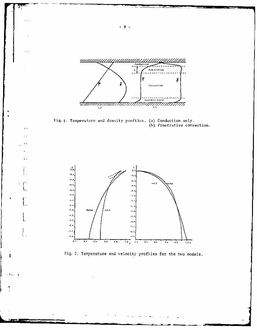
profile is distorted (Fig. 1): the initially stable region is deeply penetra- I

ted by the denser water, and is compressed until the temperature gradient isp

sufficient to produce the heat flux required for a steady state in the entire

layer; the convective region is nearly homogeneous, limited on its top by the

-7-

penetration layer and on its bottom by the intermittent, unstable layer where

the thermals are generated. The stability and initial finite amplitude behav-

ior of this system have been studied by Veronis (1963). Using the stability

criterion and the property of constant heat flux throughout the layer, Malkus

(1963) determined" the ratio of the depth of the convective region to the

total layer thickness, and the Nusselt number, as functions of a Rayleigh

number. Moreover, making some assumptions, he was also able to determine the

thickness of the penetration layer as well as its temperature profile. His

assumptions and results will be compared to the present attempt. Moore and

Weiss (1973), extending Malkus' first results, used global arguments and

showed that for Rayleigh numbers close to, but less than the critical value,

two regimes are equally likely, pure conduction or convective regime. As one

might expect, between two stable regimes exists an unstable one, and so a

third solution is found (another but less active convective regime). A

criterion of stability is built which easily leads to the instability of the

intermediate solution and to the stability of the subcritical convective

regime. The authors also built a non-linear numerical model for a

two-dimensional cell of given geometry, and compared their results.

Our interest here is not in the global heat flux relationship but in

predicting the thickness and the structure of the penetrative region.

The model of Malkus (1963) pictures the convective elements reaching

the top of the convective layer with an r.m.s. vertical velocity w and a mean

temperature excess T, such that

H con wT=v T (9)

Assuming a non-dissipative rising motion, T does not change through the

layer, it will also be considered small. As thermals penetrate, more and more

of the constant heat flux is taken over by conduction, the total heat flux

reads:

H K -IC + T :; (10)

with, at the bottom,

H w Wmax T (pure convection) (1

and at the top,K

H = K (pure conduction) (12)

The deceleration of the conservative convective element in the environment,

T e, is given by the Boussinesq relation:

W = (13)

when S T <,- T e(All the temperatures are measured from 4 0C).

Eliminating S T by the use of (11), considering the heat flux as given,

E~qs. (10) and (13) constitute a set of two equations for two unknowns T eand

W.e

On the other hand, our assumptions lend to (4) and (5), i.e.

H K ITA + WT-T~(4

9-

Fig. 1. Temerature an density poiesd()conucioooly(b Pnertie

ovetin

-0.2 -- - - - - - -

-0.4-

.0. -0.6- --

-1.6-

.1.0j -1.0tr nddniypofls a onuto ny

-c.0 -. 0,4

-2.2 .2.2

F .3 .20. . OJ L 04 .0 0.2 0:- 06 0.0 1.0

-10-

I .cT'Z TL (15)

where H, F and T' are constants related by H =f (T'-T (0)). Thismax e

constitutes another more accurate system for the same two unknowns.

The scaling of the above sets of equations leads to a scale for the

thickness d of the penetration layer. Indeed, let us scale the vertical

velocity w by its initial maximum value w mx, the environment temperature

T eby T 1 the order of magnitude of the unknown temperature at the top of

the layer, and the coordinate z by the unknown scale thickness d:

T.%(16)r

The pure conductive process at the top of the layer requires, by using

(10) or (14)

while the balance of (13) or (15) yields:

~hU. =(18)

Eliminating Tl, between the two previous relationships, a scale for d isL

found to be

.z . 2 j N Y3 1 9

- 11-

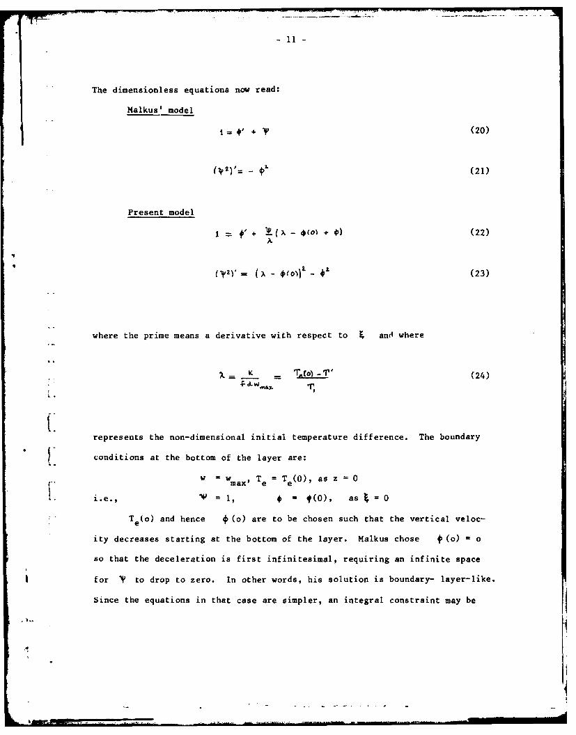
The dimensionless equations now read:

Malkus' model

=4 V * (20)

(¥L)' - (21)

Present model

+" - 4$ ( o + 4) (22)

i = + -(23)

where the prime means a derivative with respect to Fand where

K = - (24)

1..

represents the non-dimensional initial temperature difference. The boundary

'I conditions at the bottom of the layer are:

w =w max, Te T (0), as z 0

1. i.e., = 1, = (O), as = 0

T e(o) and hence * (o) are to be chosen such that the vertical veloc-

ity decreases starting at the bottom of the layer. Malkus chose f (o) = o

so that the deceleration is first infinitesimal, requiring an infinite space

for 'Y to drop to zero. In other words, his solution is boundarylayer-like.

Since the equations in that case are simpler, an integral constraint may be

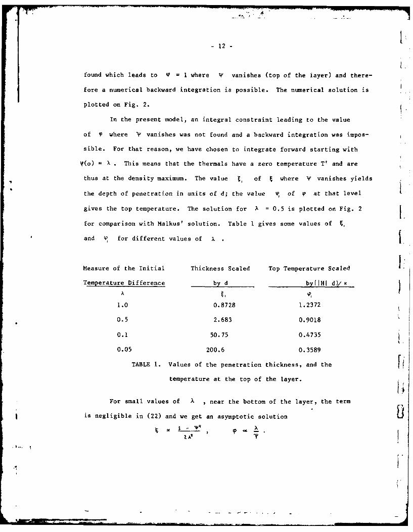
-12-

found which leads to (F' 1 where W4 vanishes (top of the iayer) and there-

fore a numerical backward integration is possible. The numerical solution is

plotted on Fig. 2.

In the present model, an integral constraint leading to the value

of V where Vf vanishes was not found and a backward integration was impos-

sible. For that reason, we have chosen to integrate forward starting with

Y(o) = X. This means that the thermals have a zero temperature T' and are

thus at the density maximum. The value t, of where Y' vanishes yields

the depth of penetration in units of d; the value tP, of lp at that level

gives the top temperature. The solution for X- 0.5 is plotted on Fig. 2

for comparison with Malkus' solution. Table I gives some values of ~

and (P for different values of x.

Measure of the Initial Thickness Scaled Top Temperature Scaled ITemperature Difference by d by(IHI d)/K

A E P

1.0 0.8728 1.2372

0.5 2.683 0.9018

0.1 50.75 0.4735

0.05 200.6 0.3589

TABLE 1. Values of the penetration thickness, and thef

temperature at the top of the layer.

For small values of ?.,near the bottom of the layer, the term

is negligible in (22) and we get an asymptotic solution

1P L__

-13-

The first relation seems to hold all across the layer and allows us to find

the value of ~.for small A when V vanishes, we get:

_5LT (25)

which is in perfec. agreement with the previous numerical solutions. This

shows that when x is small, , is no longer of order one and the variables

must be rescaled. In that case, the thickness of penetration appears to be:

thickness =-(26)2)0 4,52o

which increases if A , i.e., T (o), decreases. This is understandable

since a small T e(o) implies fast moving thermals of low beat content which

* penetrate deep into the stable region.

While there is no value of X for which the two models are identical,

V the value k 0.5 leads to close profiles. The velocity profile is very

similar except that, for the present model, 'Wv equals one for a finite value

of (-2.683 from the top). The curves of temperature differ, the present

model leading to a smaller temperature difference across the layer.

The advantage of the new calculations is to show that there is no uni-

versal profile of temperature, nor of velocity, but rather a series of profiles

depending upon the manner in which the convective elements hit the stable

region. The bottom instability of the convective layer selects the structure.

It also shows that for fast-moving elements the penetration becomes very deep,

and that a new scaling is necessary.

14

The Case of Ocean Surface Cooling

During the Fall and Winter, when the ocean surface is cooled insta-

bility and convection occur. A mixed layer is formed, penetrating in the

stable stratification below. This mixed layer, contrary to the diurnal thermo-

dline formation, is generally very efficient and may mix, in some cases, the

top 500 m of the water column. The wind stirring may play an important role

at the start but rapidly convection dominates the processes, supplying, by

itself, the kinetic energy required for stirring and deepening. In this

present attempt, we will therefore ignore the wind effect. At the bottom of

the mixed layer is the penetration layer; this layer too, deepens with time

and entrainment is present. In this case molecular conduction of heat is not

important and, in the penetration layer, the convective heat flux is progres-

sively consumed for changing the temperature of the water. Our interest is

again in predicting the thickness and the structure of the penetration layer,

by modelling the convection by thermals sinking from the surface down to thej

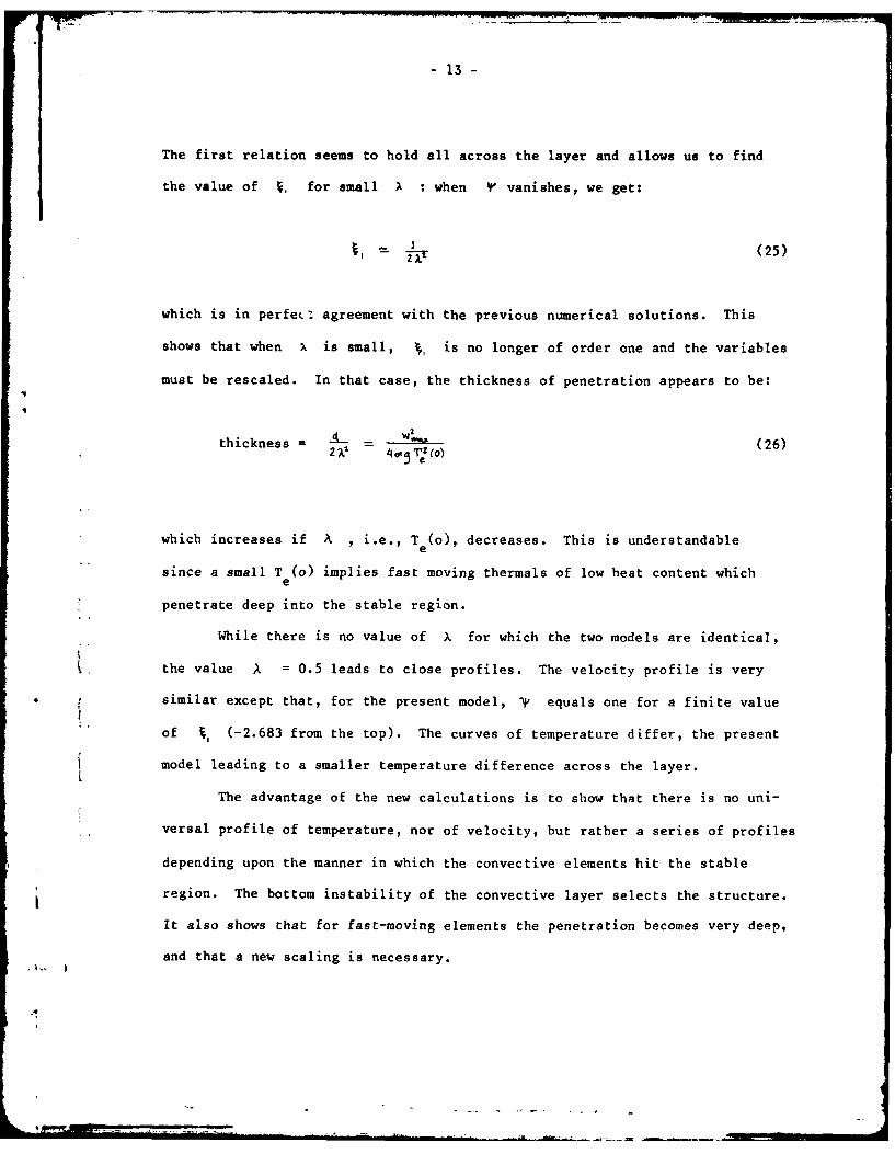
stable fluid. The situation may be depicted as on Fig. 3.

Apart from a thin unstable layer near the surface, the mixed layer of

depth h is considered of homogeneous temperature T 0. This layer is progres-

sively cooled and thus leads to a linear decrease of the heat flux from its

imposed surface value Q (Q ) o for cooling). In the unstable layer, con-

vective elements are produced with a temperature T',,during their sinking

motion they gradually mix with their environment and T' becomes closer to

T 0. When the temperature profile curves, the temperature will first equal

and then exceed the environmental temperature, there noted by T .Where T'

Tealmost at the top of the penetration layer, the convective heat flux is

exactly zero, according to (4). In the penetration layer, the convective

-15-

,-0 ,0 a

Sunstlable layr--------- ------------------------------- ---- -

/

ixed yr 110

Fig. 3. Schematic diagram of the temperature and heat fluxprofiles in case of penetration in a stable ocean

by surface cooling.

I M 0 .2 .4 .6 .8 .

(z.O) '

f2 2it Teperat- AE ," - (1_6C2

,"¢ ! the t!l-mals

(R(E

,~Ieat flu..

(.......... ----- -- --------

2. 1.9 1.6 1.4 ,8 .6 .4 .2 0 .2 .4 .6 .8 1.

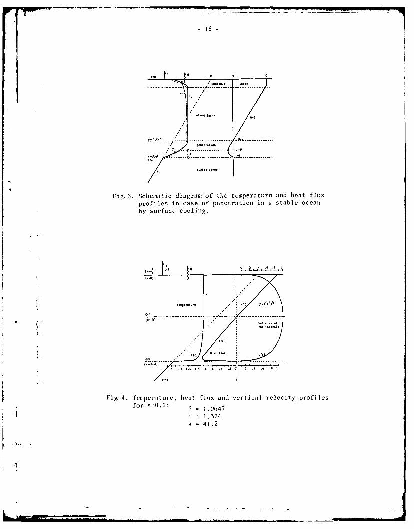
1.4c

Fig. 4. "Temperature, heat flux and vertical velocity profilesfor s=O.1; 6 1.0647

1. 324A = 41.2

. ''W OMB

/9+

-16-

elements are warmer than their surroundings, the heat flux is therefore down-

ward (negative) and they decelerate. The time scale of the entrainment process

is much greater than the time required for an element to sink all the way down.

We may therefore assume that an element sees a steady temperature profile and

stops exactly at the bottom of the penetration layer. According to (4), the

convective heat flux, there again is zero. If we neglect the conduction, the

heat flux exhibits the profile shown on Fig. 3, with a negative minimum value

inside the penetration layer.

The heat conservation equation is:

(27)

and tells us that above the minimum value of H the temperature decreases while

beneath the minimum it increases with time. A short time after, the tempera- Iture profile will look like the dotted profile on Fig. 3. Somewhere in the

penetration layer, Te did not change. Of course that level deepens with

time, allowing every level of fluid to be cooled after a short time of heating.

Above the intersection point of the T' and T e profiles, the convective

elements are denser than their environment. They thus accelerate and mix with

the surroundings, equations (6) and (8) hold. Below that point, the elements

are less dense and decelerate; there equations (7) and (8) are to be used; the

temperature T' is therefore constant, approximately equal to T (see Fig. 3).0

In the present model we will assume that the changes in temperature follow the

deepening, having in mind the search of a similarity solution. We note

T 0=T' - -E rh (28)

T e-n f(~ (29)

17 -

where r is the temperature gradient in the stable layer, £ a pure number

to be determined by the model, f( 4 ) an unknown function of the similarity

coordinate through the penetration layer (see Fig. 3).

0 at the top of the layer

at 1 at the bottom of the layer

must match the temperature profiles above and below the penetration layer,

i.e.,

f(O) = £ , f(l) - 1 + d. (30)

For similarity to be used, the last condition requires that d grow in time as

h does. We therefore note:

d = S (31)

where S is a second pure number to be determined by the model.

Firstly, a few properties inside the mixed layer will be deduced to

help to solve the penetration dynamics. Then, the equations for the pene-

tration will be established, an integral constraint, found, and a numerical

solution presented. Finally, an analytical solution will be given for the

case of strong initial stratification, and this solution will be compared to

the model of Krauss and Turner (1967).

A Few Properties Inside the MixedLayer:

In the mixed layer the temperature T0 is z-independent and the heat

conservation equation (27) may thus be integrated to find the heat flux:

(32)

where Q is the surface value considered as the forcing of the system. Using

18 -

(28) and the fact that H vanishes at the bottom of the mixed layer (z =-h),

we get:

Q = E r h. (33)

If Q may be considered constant and if h is initially zero, we may integrate

and find h at any time, provided that C is known.

We neglect any conduction, assuming it plays a negligible role in the

entrainment process. The definition of the heat flux (4) and the equation of

motion (5) may be solved with the use of (32) and (33) to get:

w"S= "10) + + f

tr (k+ t)

where N = o fr is the Brunt-Vaisala frequency in the stable layer. For a

mixed layer deep enough, at the bottom of the layer the value w (z=0) has no

effect, and we getw(-h_- (34)

T '(- = -Eri.k (35)

The latter relationship is a repetition of (28) and gives the temperature T

across the penetration layer.

- 19-

The SimilarityEquations_ For_ the Penetration Layer:

We introduce in place of T e H and w the similarity functions f( Y,e

( ) and v ( ) such that:

T = - fhf( )e

H = - Qg( P ) = - fhlg( 4 ) (36)

w =-hNv( )

and we also introduce a dimensionless measure of the underlying stratification:

= ,14 (37)

The equations (4), (5) and (27) yield:

- (38)

v f {((- £39)

+ &-) .((),)-= - '((40)

The boundary conditions are:

-at the top:

=0 f(0)--

v(O) = (41)

g(O) = 0

EbbI

-20-

- at the bottom + =1 f(1) - 1 3

v(1) 0 (42)

g(l) 0. i

According to (38), the two conditions on g( ) are redundant. Equation (38)

is algebraic;. the system is of second order and required only two boundary

conditions. We are thus left with two extra conditions, precisely those which

will enable us to determine E and S. The problem is therefore closed and

self-consistent.

Replacing f( ) by its expression from (39) into (40), we may

integrate with respect to . and use the top boundary conditions (41):

- v - E 3 ('P) . . (43)

Using the bottom boundary conditions (42), we obtain a relationship between

and

61 3j 0.(44)

This i's an integral constraint. It may be shown that it is identical to the

global heat budget of the system: the amount of heat lost at the surface was Iiused to cold the fluid from its initial stratification to its present state: U

Qd(l - " a%l o -'-a i"

ii - il a I i r- . - F " ' :-, :jl±-: , " .... . li II II I I

-21-

On the other hand, looking at the conversion of potential to kinetic energy we

are led to consider the integral

0 0

;;T at H ai4z

The computations reveal that the integration across the mixed layer exactly

balances the integration across the penetration layer, leading to a net zero

global conversion. This is understandable: since the model is conservative

(inviscid and nonconducting), the potential energy in the mixed layer is given

to the accelerating thermals and recovered in the penetration layer where the

thermals decelerate. Because there is no conversion, no dissipation and no

energy impact from the wind, the total kinetic energy in the system is

conserved. But, the kinetic energy in the mixed layer always increases with

time.

From (38) and (39), we may express g( Fe ) and f( in terms of N( )

Replacing in (43), we end up with a single first-order nonlinear differential

equation:

V2 ( t FSk t0.

A Numerical Solution

If we were able to solve analytically that equation by using the top

boundary condition on v, we could find the second relationship between 'j

and S by using the bottom boundary condition on v. But this is not the case

and the problem must be addressed in a different way if we want to find a

A".

-22-

numerical solution. For that purpose let us note:

VSt (44)

= (47)

s= (48)

and the problem becomes:

(49)I' + - + 1 0 [

with

u = 1 as V= 0 (50)

u W 0 as = S (51)

The coefficient s contains the unknown f and the known X . Let us

assign a value to s, and set X free, so that we may solve (49) with the aid

of (50). The value S of where u vanished will be given by the numerical

M

-23-

solution. Going back to the integral constraint (44) transformed into

(52)

+ 2(1- Os+ (I(fsp= 0

we solve for E Finally, the definition of s will tell us for which value

of ?X the solution was found.

Calculations were carried out for the value s = 0.1. The solution as

well as the analytical solutions for the mixed layer are shown on Fig. 4. The

penetration layer is found as thick as the mixed layer C£very close to one)

but the variation in temperature and heat flux are concentrated near the

bottom of the layer. This might be surprising but will be understood in light

of the analytical solution for the asymptotic case of strong underlying

stratification.

The Case-of Strong-Underlying Stratification

According to (37) and (48), strong stratification in the stable layer

(large Brunt-Vaisala frequency) leads to a small value of s. (A small rate of

entrainment h leads to a small value of s, too). The present paragraph is

devoted to finding an asymptotic analytic solution for s close to zero.

For s = o, equation (49) joined to u( ~ 0) = 1, yieldb the solution

u3 rL2 (53)

which is, by the way, exactly the solution in the mixed layer. The solution

leads to an unbounded bracketed quantity in (49) near rL= 1. We have thus

to consider a boundary layer near ' = ,anticipating that 5 is close

to unity. Scaling arguments show that in the boundary layer, u is of order s

- 24 -

and S - of order s3 . The solution satisfying u( - S ) o is found

to be: ju3 + s(l+ 8 )u2 = 2 & ( (54)

This solution for increasing u and -L must match the interior solution

(53) for small u and S -Y The matching implies

(55)

and the two solutions may be combined to yield a simple expression valid

throughout the layer to order s:3 2 2

u + 2su 2 = 1-11. (56)

The use of the integral constraint (52) gives, to first order

_/2, (57)

and therefore the solution is found for large values of x g-.ven by

(58)

Back to the initial variables, the solution reads:

Xv3 + 3v' " - ( ,. (59)

* f ( 4 + ) (60)3t )L, +

- 25 -

(61)It

3.

The thickness of the boundary layer was found to be s in units

of v . Back to the variable z, the actual thickness is (without a factor

27

t (62)h t

inversely proportional to N 2 . The larger the underlying stratification,

the thinner the boundary layer and the sharper the transition between pene-

tration and stable fluid.

The thickness t is to be considered as the thickness of the thermocline.

So, by this model we are led to establish a distinction between penetration

layer and thermocline. The penetration is a layer as thick as the mixed

layer, and is usually incorporated in the latter from a double layer, theVso-called "mixed layer". The thermocline, on the other hand, is a thin region

of large transition, the front of the penetration.

It is worthwhile to confront the solution of Krauss and Turner (1967)

with the present asymptotic case. They model the "mixed layer" as homogeneous

bounded below by an infinitely sharp thermocline. Their model contains two

unknowns: the depth h of the mixed layer and its temperature T . The first

equation they use is identical to (32). To form their second equation they

-26-

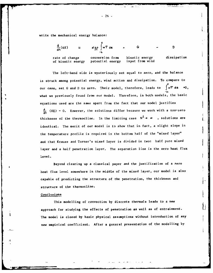
write the mechanical energy balance:

(K= 1 WT': + Gr D

rate of change conversion from kinetic energy dissipationof kinetic energy potential energy input from wind

The left-hand side is mysteriously set equal to zero, and the balance

is struck among potential energy, wind action and dissipation. To cmpare to

our case, set G and D to zero. Their model, therefore, leads to JwT da =0,

what we previously found from our model. Therefore, in both models, the basic

equations used are the same apart from the fact that our model justifies

4 (KE) = 0. However, the solutions differ because we work with a non-zero

thickness of the thermocline. In the limiting case Nt Z_# 0 solutions are

identical. The merit of our model is to show that in fact, a slight slope in

the temperature profile is required in the bottom half of the 'mixed layer'

and that Krauss and Turner's mixed layer is divided in two: half pure mixed

layer and a half penetration layer. The separation line is the zero heat flux

level.

Beyond clearing up a classical paper and the justification of a 7ero

heat flux level somewhere in the middle of the mixed layer, our model is also

capable of predicting the structure of the penetration, the thickness and

structure of the thermocline.

Conclusions[

This modelling of convection by discrete thermals leads to a new

approach for studying the effects of penetration as well as of entrainment.

The model is closed by basic physical assumptions without introduction of any

new empirical coefficient. After a general presentation of the modelling by

-27

convective elements, the model was applied to steady and unsteady cases. In

the study case of water cooled below 40C on its bottom, the structure of the

penetration was compared to a previous model (Malkus, 1963), and we pointed

out the non-universality of that structure and its dependence upon the bottom

instability. In the non-steady case of the mixed layer deepening, the model

leads to a penetration layer as thick as the mixed layer. Therefore, the

so-called mixed layer as we observe it has in fact a double structure and

contains the pure mixed layer and the penetration layer. For a strong

underlying stratification, the model predicts a sharp thermocline, front of

the penetration layer.

This model is to be understood as a compromise between depth integrated

models with an infinitely sharp thermocline (Krauss and Turner, 1967; Pollard,

Rhines, and Thompson, 1973; Heidt, 1977), and more elaborate numerical models

where the full partial differential equations are solved for a particular

geometry (Moore and Weiss, 1973). By its situation of a compromise and its

physical background (convective elements are actually observed), the model may

be fruitful, especially if certain weaknesses are removed and improvements

made.

Among the weaknesses are the assumptions of identical thermal elements

and the absence of wind and shear effects. In the mixed layer deepening case,

the assumption of crossing and profiles exactly where T starts to curve

might be reconsidered. Indeed, in the limiting case of strong underlying

stratification, the curvature of the T eprofile is trapped in the thermo-

dline.

Among the possible improvements as starting points for a future work,

we propose to relax the assumption of identical elements by introducing property

-28

L.

distributions and a statistical treatment. We also plan to ivestigate the

generation of internal gravity waves in the penetration layer, and to study

the case of a more general relationship between volume and velocity.

Acknowledgments

My sincere thanks go to Professor Malkus for suggesting to me the

problem. His continuous guidance throughout this work is deeply appreciated.

I am grateful to the Staff Members for giving me the chance to participate in

the GFD summer program and for financial support.

REFERENCES I.

Furumoto, A. and Rooth, C., 1961. Observations on convection in water cooledfrom below. Geophysical Fluid Dynamics, Woods Hole OceanographicInstitution, WHOI-61-39(3). i

Heidt, F. D., 1977. The growth of the mixed layer in a stratified fluid due

to penetrative convection. Boundary Layer Meteorology, 12, 439-461.

Krauss, E. B. and Turner, J. S., 1967. A one-dimensional model of theseasonal thermocline, II. Tellus, 19, 98-105.

Malkus, W.V.R., 1963. A laboratory example of penetrative convection. Proc.3rd. Tech. Conf. on Hurricanes and Tropical Meteorology, Mexico, W-95.

Manton, M. J., 1975. Penetrative convection due to a field of thermals. Jour.Atm. Sci., 32, 2272-2277.

Moore, D. R. and Weiss, N. 0., 1973. Nonlinear penetrative convection. Jour.Fluid Mech., 61, 553-581.

Pollaid, R. T., Rhines, P. B. and Thompson, R., 1973. The deepening of thewind-mixed layer. Geophysical Fluid Dynamics, 4, 381-404.

Turner, J. S., 1973. Buoyancy effects in fluids. Cambridge Univ. Press,367 p.

Veronis, G., 1963. Penetrative convection. Astrophys. J., 137, 641-663.

.4

-29-

PENETRATIVE CONVECTION BEHIND A MOVING,

HORIZONTAL TEMPERATURE DISCONTINUITY

Richard E. Moritz

I. Introduction

The motivation for this study comes from a desire to better understand

the sea-to-air energy exchange processes over isolated openings (e.g. leads or

polynyas) in an otherwise continuous canopy of sea ice. Given that a stably-

stratified shear boundary layer comprises a typical upstream boundary con-

dition, one is confronted with the problems of penetrative convection and

shear turbulence in a horizontally-inhomogeneous internal boundary CIBL)

(Venkatram, 1977). A simpler problem, requiring fewer assumptions and empiri-

cal parameters, is obtained by eliminating the effects of mean shear flow so

as to isolate the problem of convective heat transfer due to buoyancy. While

we may not expect quantitative agreement between the latter model and measure-

ments in the pack ice (because the shear flow is undeniably crucial to heat

fluxes in the real atmosphere), it is the author's opinion that the simpler

problem is interesting in its own right and can provide insight into the more

complete problem. A significant component of the physics is retained here,

namely, the internal boundary layer processes associated with penetrative

convection in an initially stable fluid. Moreover, a well-established theory

for the heat flux is available, requiring only two empirical constants, both

of which are known from careful laboratory experiments. Finally, a controlled

laboratory simulation of our model IBL may be feasible, so that the

conclusions might be subject to verification. In the next section we describe

the simple convective system to be studied.

-30-

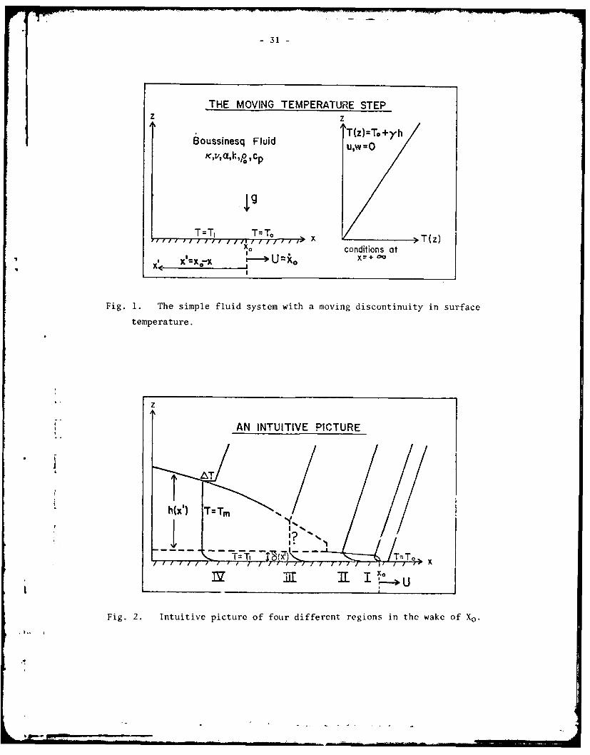
II. The Moving Temperature Discontinuity

Consider a two-dimensional "Boussinesq" fluid system in the (x,z) plane

(Fig. 1). We assume that the fluid is at rest (u,w 0) and is linearly

stratified (T(z) = T0 + Yz) at x = + 0O Here T is the fluid temperature,

is a constant vertical temperature gradient, (u,w) are the (x,z) velocity com-

ponents and T is the surface temperature at x = + 00 The fluid is acted0

upon by a body force field (0,g) and is completely characterized by its mean

density , , specific heat capacity (at constant pressure) c , thermal con-Q0 p

ductivity k, thermal diffusivity K = k/oC p, molecular viscosity V and

thermal expansion coefficient o (all assumed constant). Hence our equation

of state reads

(i-TT') (1)

I

where T'- T-T,

and P is a convenient reference pressure. Equation (1) corresponds to a0

linear decrease in density with height at x = + 00 that can be characterized

as hydrostatically stable by incorporating the assumed state of rest and the

body force g into the z-momentum equation. Thus Y is our stability para-

meter. We imagine that the system is a half-plane, bounded at z = 0 by a

smooth, perfectly conducting plate. At the moving coordinate x x (t) is

maintained a step change in the temperature of the plate, such that T(x,0,t) -

T for x > x and T(x,0,t) = T > T for x 4 x . This tempera-o o o,.. ture discontinuity moves along the plate at constant speed U = where C * )

0

.4

- 31

THE MOVING TEMPERATURE STEPz z

oussinesq Fluid T(z)=T.+Yh

KIVIC1110u,W=O

T:Tj T=:TO/ ,,,,,TrT 0 , , ,> x T(z)

xo conditions atx = X l; x -- U = i o X =+ e

9 IX.C

Fig. 1. The simple fluid system with a moving discontinuity in surface

temperature.

z

AN INTUITIVE PICTURE

TATNOx T=Tm

.1 / iT44

,,T - ,? -. 7X 0

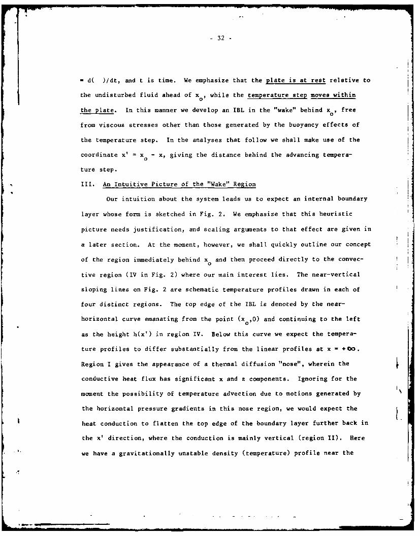
Fig. 2. Intuitive picture of four different regions in the wake of Xo .

...1 - - -- _

-32-

=d( )/dt, and t is time. We emphasize that the plate is at rest relative to

the undisturbed fluid ahead of x 0, while the temperature step moves within

the plate. In this manner we develop an IBL in the "wake" behind x 0, free

from viscous stresses other than those generated by the buoyancy effects of

the temperature step. In the analyses that follow we shall make use of the

coordinate x' =x - x, giving the distance behind the advancing tempera-

ture step.

III. An Intuitive Picture of the "Wake" Region

Our intuition about the system leads us to expect an internal boundary

layer whose form is sketched in Fig. 2. We emphasize that this heuristic

picture needs justification, and scaling arguments to that effect are given in

a later section. At the moment, however, we shall quickly outline our concept

of the region immediately behind x 0and then proceed directly to the convec-

tive region (IV in Fig. 2) where our main interest lies. The near-vertical

sloping lines on Fig. 2 are schematic temperature profiles drawn in each of

four distinct regions. The top edge of the IBL is denoted by the near-

horizontal curve emanating from the point (x,0) and continuing to the left

as the height h(x') in region IV. Below this curve we expect the tempera-

ture profiles to differ substantially from the linear profiles at x = + 00.

Region I gives the appearance of a thermal diffusion "nose", wherein the

conductive heat flux has significant x and z components. Ignoring for the

moment the possibility of temperature advection due to motions generated by

the horizontal pressure gradients in this nose region, we would expect the

heat conduction to flatten the top edge of the boundary layer further back in

the x' direction, where the conduction is mainly vertical (region II). Here

we have a gravitationally unstable density (temperature) profile near the

- 33 -

plate, giving way to the linear, stable gradient X above the edge of the

IBL. Further behind the step x the diffusion has had more time (t = x'/U)0

to thicken the thermal boundary layer, which eventually reaches a height z

- at which the growth rate of (convectively unstable) perturbations is no

longer negligible relative to the diffusive growth rate K/&(Howard,

1964). At this point vertical convection sets in, in.earnest, penetrating

the overlying fluid (region III). As the process continues, we assume that a

mixed layer, wherein temperature is effectively constant with height, develops

between the unstable surface layer (zo.. 6 ) and stable fluid above (z =

h(x')). Such layers are observed, for example, in penetrative convection in

laboratory tanks (Heidt, 1977), the essential difference being that we have

assumed a similar process in a system with horizontal variations. Again, our

worries about the possible horizontal circulation set up by the horizontal

temperature gradient will be deferred. At some point, then, we enter region

IV, within which h(x') is so much larger than the local thermal boundary layer

thickness ( x') that we can adopt the "1/3 power law" for the Nusselt number,

namely

Nu = cRaI/3 (2)

The Nusselt number is defined as the ratio of the total vertical heat flux H

in the freely-convecting region to the flux that would occur by conduction

alone acting on the vertical mean temperature gradient. If T is defined tof m

be the mixed layer temperature then

(3)

NLA [ (T T .---Jl k(

- 34 -

I -

The Rayleigh number Ra is given here by

(T. - r) 4

while c is an empirically-determined constant (that may, however, vary with

the Prandtl number Cr = V/j . The "1/3 power law" is the only com-

bination that makes the heat flux H independent of the height h(x') as h--0

(Stern, 1975), as is easily seen by combining (2), (3) and (4) and solving for

H. Once more we defer until later questions involving the production of shear

by the convection itself in such a way as to alter the heat flux in a way that

depends on h and Or . We now consider the convective region IV in more

detail.

IV. The Penetrative Convection Region

We now focus our thoughts on region IV (Fig. 3). For convenience sake

we have here reversed the directions of the horizontal coordinates, so x' now

increases to the right and x0 moves to the left with speed U. In order to

obtain a tractable mathematical representation of the system, we adopt the

idealized geometry and temperature profile shown in Fig. 3. In the lowest

layer (0 -C z S ) the vertical heat transport is accomplished chiefly by

molecular conduction and a correspondingly large fraction of the total mean

temperature difference across the system is therefore confined to this

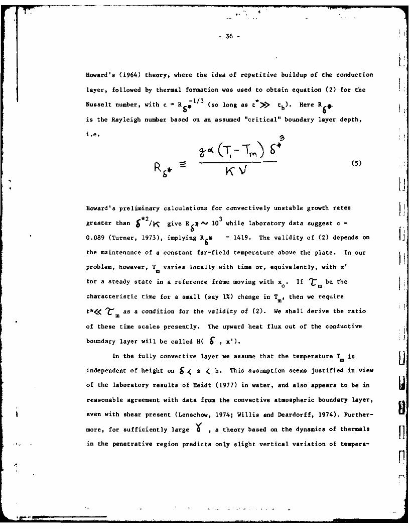
stratum. At the top of this layer there is convective activity in the form of

intermittent "thermals"-plumes of heated boundary layer fluid which, when

sufficiently unstable, rip away from the plate, as shown schematically in

Fig. 4. Laboratory experiments in air (Townsend, 1959) and water (Heidt,

1977) demonstrate clearly the existence of the thermals. Figure 4 is based on

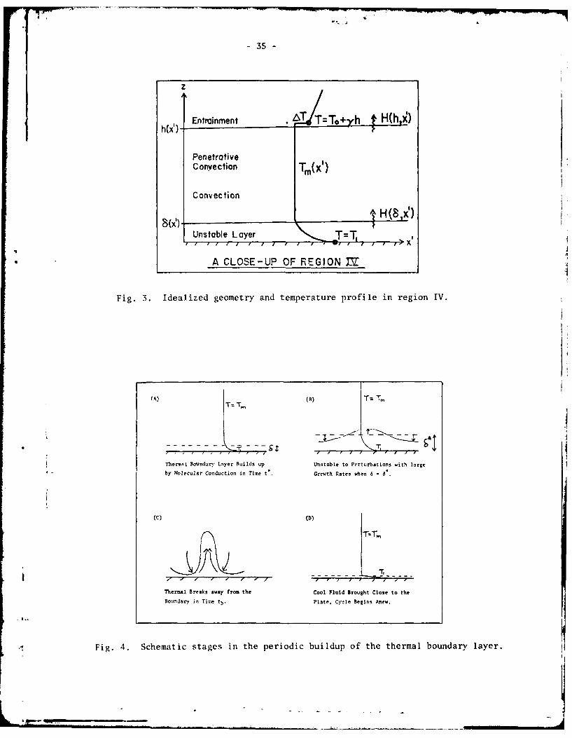
35 -

Entrainment . =T To xh H(h, x)

Penetrative

Convection Tm(X')

ConvectionS~x)I H (8,x )

Unstable Layer TTI I '1 1 I I /I I I X

q A CLOSE-UP OF REGION

Fig. 3. Idealized geometry and temperature profile in region IV.

SThermil Boundary" Layer Builds up Unstable to Perturbations with large

• by Molecular Conduction in Time re, Grow'th Rates when 6 - 6'.

(C) (D) Tf / / f I j '< f _

T-TII

Theral Breaks away fra the Cool Fluid Brought Close to the

Boundary in Tine tb. Plate, Cycle Begins Anew.

Fig. 4. Schematic stages in the periodic buildup of the thermal boundary layer.

- 36 -

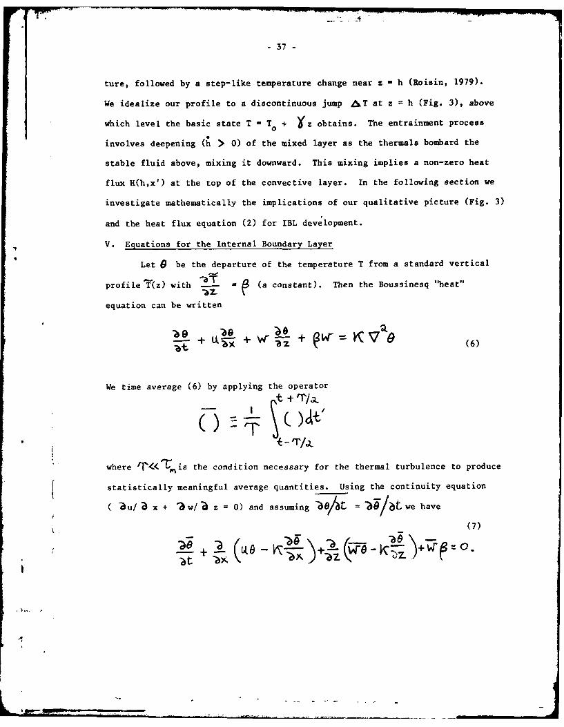
Howard's (1964) theory, where the idea of repetitive buildup of the conduction

layer, followed by thermal formation was used to obtain equation (2) for the

Nusselt number, with c = R 1 /3 (so long as t>> tb). Here R 6 *

is the Rayleigh number based on an assumed "critical" boundary layer depth,

i.e.

R K Vii

Howard's preliminary calculations for convectively unstable growth rates

greater than *2 /K give R# F- 103 while laboratory data suggest c

0.089 (Turner, 1973), implying R i = 1419. The validity of (2) depends on

the maintenance of a constant far-field temperature above the plate. In our

problem, however, T varies locally with time or, equivalently, with x'm

for a steady state in a reference frame moving with x0 . If 7 be the

characteristic time for a small (say 1%) change in Tm, then we require

t*<< 7m as a condition for the validity of (2). We shall derive the ratio

of these time scales presently. The upward heat flux out of the conductive

boundary layer will be called H( 6 , x').

In the fully convective layer we assume that the temperature Tm is

independent of height on S/, z < h. This assumption seems justified in view

of the laboratory results of Heidt (1977) in water, and also appears to be in

reasonable agreement with data from the convective atmospheric boundary layer,

even with shear present (Lenschow, 1974; Willis and Deardorff, 1974). Further-

more, for sufficiently large * , a theory based on the dynamics of thermals Hin the penetrative region predicts only slight vertical variation of tempera-

., p , • ' , _ , . . . .. .... . . -

- 37 -

ture, followed by a step-like temperature change near z h (Roisin, 1979).

We idealize our profile to a discontinuous jump AT at z = h (Fig. 3), above

which level the basic state T = T + Yz obtains. The entrainment process

involves deepening (h > 0) of the mixed layer as the thermals bombard the

stable fluid above, mixing it downward. This mixing implies a non-zero heat

flux H(h,x') at the top of the convective layer. In the following section we

investigate mathematically the implications of our qualitative picture (Fig. 3)

and the heat flux equation (2) for IBL development.

V. Equations for the Internal Boundary Layer

Let 9 be the departure of the temperature T from a standard vertical

profile f(z) with - = (a constant). Then the Boussinesq "heat"

equation can be written

'b i e , + K=it- bxV TZ(6)

We time average (6) by applying the operator

t I-/a

,- Iwhere fr< is the condition necessary for the thermal turbulence to produce

statistically meaningful average quantities. Using the continuity equation

Zu/ Z x + '3w/ z = 0) and assuming Td1t = /btwe have

(7)

at -ax

* b..

.4I

-38-

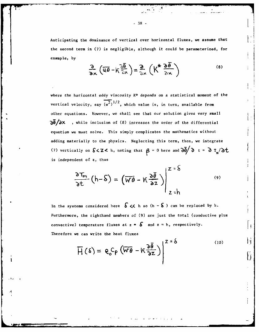
Anticipating the dominance of vertical over horizontal fluxes, we assume that

the second term in (7) is negligible, although it could be parameterized, for

example, by

10C)

where the horizontal eddy viscosity K* depends on a statistical moment of the

vertical velocity, say 7w-2)1/, which value is, in turn, available from

9 other equations. However, we shall see that our solution gives very small

X while inclusion of (8) increases the order of the differential

equation we must solve. This simply complicates the mathematics without

adding materially to the physics. Neglecting this term, then, we integrate

(7) vertically on C/, Z- h, noting that =0 here andO/ t T m ,~~

is independent of z, thus

In the systems considered here C <h so (h - )can be replaced by h.

Furthermore, the righthand members of (9) are just the total (conductive plus

convective) temperature fluxes at z = 6'and z h, respectively.

Therefore we can write the heat fluxes

- (10) L

-39-

and

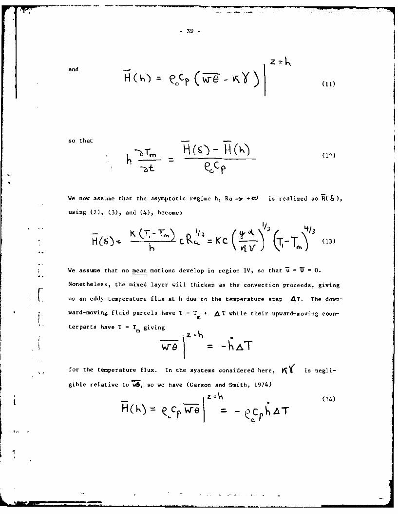
so that

We now assume that the asymptotic regime h, Ra -) +CO is realized so H(S),

using (2), (3), and (4), becomes

H, C KC - (i-T') (13)

We assume that no mean motions develop in region IV, so that = = 0.a.

Nonetheless, the mixed layer will thicken as the convection proceeds, giving

[ us an eddy temperature flux at h due to the temperature step AT. The down-

ward-moving fluid parcels have T = Tm + AT while their upward-moving coun-

mm"terparts have T = T mgiving

for the temperature flux. In the systems considered here, K is negli-

gible relative tc _j, so we have (Carson and Smith, 1974)

HN = cp = - c T (14)

- 40 -

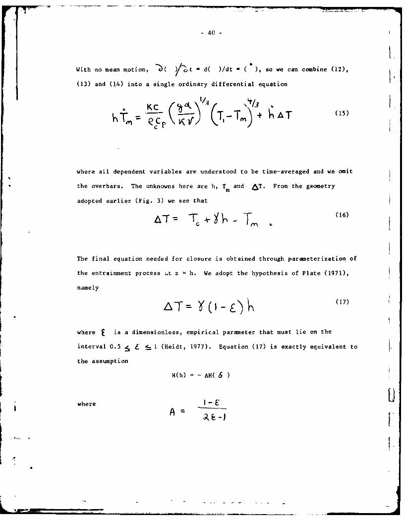
With no mean motion, ( t d( )/dt = ( ), so we can combine (12),

(13) and (14) into a single ordinary differential equation

i

.- 1 f/3 A (15)

where all dependent variables are understood to be time-averaged and we omit

the overbars. The unknowns here are h, Tm and &T. From the geometry

adopted earlier (Fig. 3) we see that

,67 T (16)

The final equation needed for closure is obtained through parameterization of

the entrainment process t z = h. We adopt the hypothesis of Plate (1971),

namely

~ ~'i-5)k(17)

where E is a dimensionless, empirical parameter that must lie on the

interval 0.5 r_ 1 (Heidt, 1977). Equation (17) is exactly equivalent to

the assumption

H(h) = - AH( )

where _- UA - I"

- 41 -

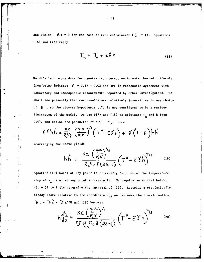
and yields AT - 0 for the case of zero entrainment (E = 1). Equations

(16) and (17) imply

0 (18)

Heidt's laboratory data for penetrative convection in water heated uniformly

from below indicate 6 = 0.87 + 0.03 and are in reasonable agreement with

laboratory and atmospheric measurements reported by other investigators. We

shall see presently that our results are relatively insensitive to our choice

of £ , so the closure hypothesis (17) is not considered to be a serious

limitation of the model. We use (17) and (18) to eliminate T and h fromm

(15), and define the parameter T* = T - T0, hence

1 C

Rearranging the above yields

~ ((A &-I* (Ta 5/3 (19)

'Q 'C

Equation (19) holds at any point (sufficiently far) behind the temperature

step at xo, i.e. at any point in region IV. We require an initial height

hit = 0) to fully determine the integral of (19). Assuming a statistically

steady state relative to the coordinate xo, we can make the transformation

St = = x'/U and (19) becomes

It/

S(20)

-42-

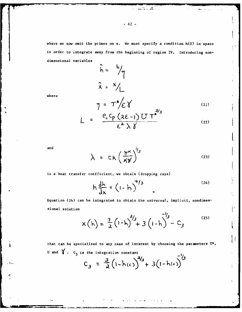
where we now omit the primes on x. We must specify a condition h(O) in space

in order to integrate away from the beginning of region IV. Introducing non-

dimensional variables

where

T (21)

L:p x ) U(22)

La.N.

and 1

X (23)

is a heat transfer coefficient, we obtain (dropping caps)

- 'i-f3 (24)

Equation (24) can be integrated to obtain the universal, implicit, nondimen-

sional solution

/jv+ ~(25)

that can be specialized to any case of interest by choosing the parameters T*,

U and Y C3 is the integration constant

-c 3 - + 3 0

- 43 -

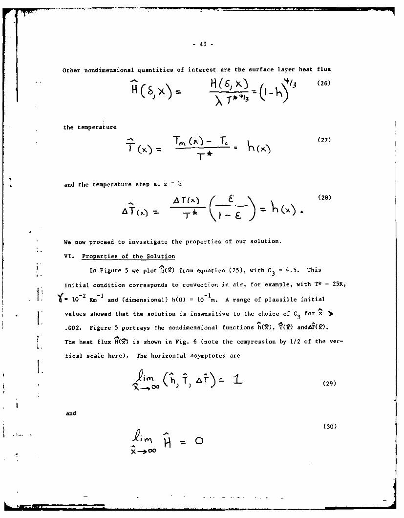
Other nondimensional quantities of interest are the surface layer heat flux

H(6,K413 (26)

the temperature

% T= T (27)T - T) = TTA

and the temperature step at z = h

AT x, (28)

* We now proceed to investigate the properties of our solution.

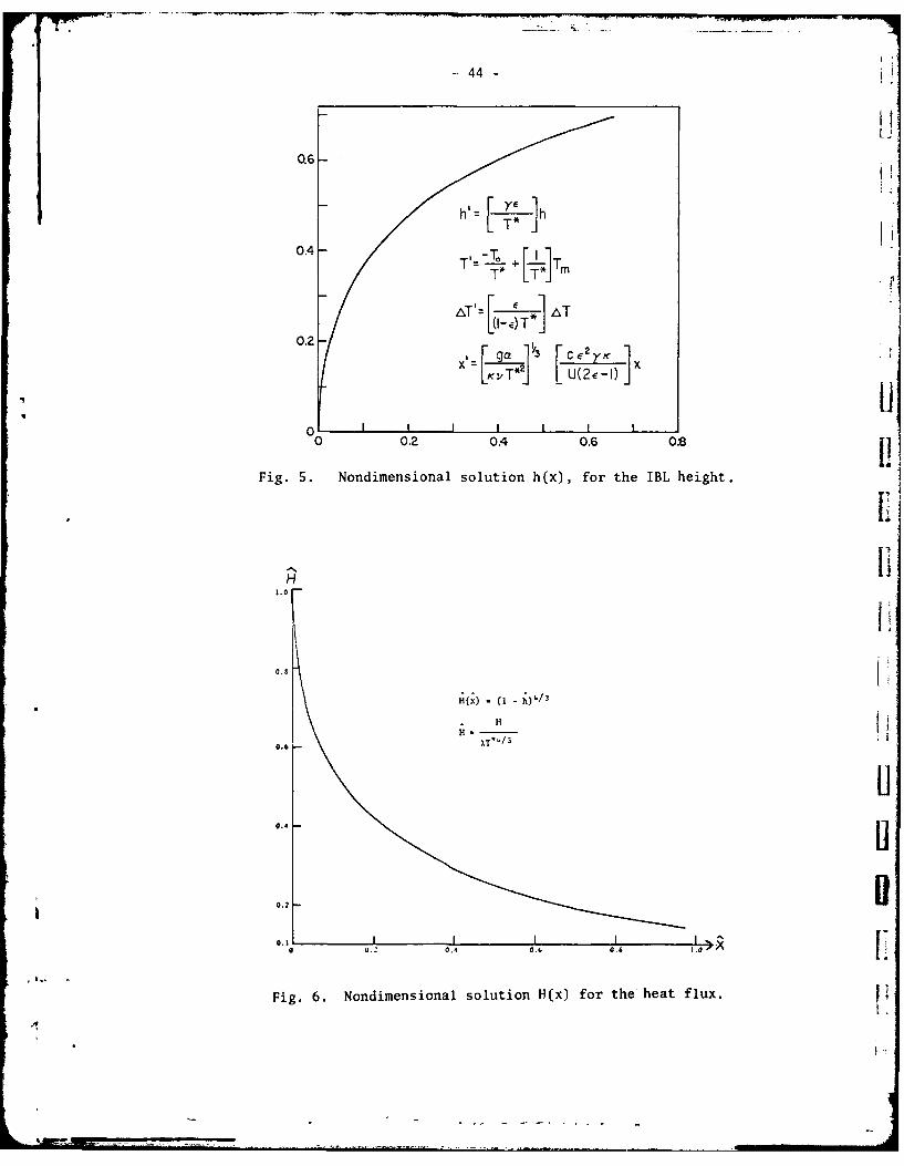
VI. Properties of the Solution

In Figure 5 we plot h(x) from equation (25), with C3 = 4.5. This

initial condition corresponds to convection in air, for example, with T* f 25K,

-2 - -1q= 10. Km and (dimensional) h(0) = 10 m. A range of plausible initial

* values showed that the solution is insensitive to the choice of C3 for x

.002. Figure 5 portrays the nondimensional functions h(S), T(5) andAX().

The heat flux %(') is shown in Fig. 6 (note the compression by 1/2 of the ver-

tical scale here). The horizontal asymptotes are

* .1 (29)

and

'.,,,, (30)

% 00

44-

LJ

.6 -

0.4 -T FIT

T

T'I U(2-I)

I I I I I I I

0 0.2 0.4 0.6 0.8

Fig. S. Nondimensional solution h(x), for the IBL height.

H

0.6 LT

0.4 s

0.2 D

0 0. 0.4 0.6 0.6 .

Fig. 6. Nondimensional solution H(x) for the heat flux.

45 -

corresponding to h-- T*/F , Tm - TI, AT-T*(1- F /C ) and H--* 0,

all as x -- V . Note that H(O) = 2T* 4 /3 . We can see from the plots

that all variables change rapidly with x near x = 0, which point corresponds

to the temperature step, x0 . If we define X n as the nondimensional

distance from x to x (the analog of "fetch" if the fluid were moving at0

speed U) at which a dependent variable has changed by a factor n of the

difference between its initial and asymptotic values, then

• . ,, ) = .2

((1

o ;L .O (33)

and

(34)

where the superscripts denote the dependent variables. In order to assess the

qualitative significance of these numbers, we must multiply by the length scale

L. First, however, let us note the qualitative dependence of 11 , the asymp-

totic mixed layer height, and L on the parameters of the problem. From (22)

we have L proportional to the heat capacity e cp, and inversely relatedto the heat transfer coefficient ;. The combination (21 - _ and the

parameter UT*2/ 3/ 1 (as given in any particular problem) also vary directly

as L. The former quotient increases from 0.76 to I as S is varied from 0.67

- 46 -

to 1, so our choice of is not crucial within wide limits as regards the

qualitative analyses of L that follow.

As one might expect, the maximum height i is proportional to the tem-

perature difference T* and inversely proportional to . Thus a hotter sur-

face heats a deeper layer, but the stability can confine the mixing. One

interesting effect of f is to keep the heat capacity 9 cph of the mixed

layer smaller, leading to larger temperature changes for a given heat flux.

The heat flux scales with X T*4 /3 , independent of Y. For this reason,'II

then, L is inversely proportional to and a larger stability implies a

smaller "fetch" required for significant changes in h, Tm, T and H. L

also varies directly with U, which might be viewed as the analog to the rate

of cold air input to the heated lead. When this rate is large, a longer fetch

is required to attenuate the heat flux and vice versa. The dependence of L on

T*2 is a direct consequence of equation (2) for the Nusselt number. A

different power of T* determines the length scale when the transfer of heat by

shear turbulence is parameterized in a simple way as we shall see shortly.

Despite the rather questionable correspondence between our -nodel IBL

and a real flow over leads, we can adopt the following values characteristic

of the lead problem in winter

. = 1.11 - 0 K Sm

ICT k ;

and see what happens. The resulting length scale is

L = 4769 Km

- 47 -

so for exampleXY. is 114 km. Although wintertime open water features onY I

such a scale have been observed in the Arctic (Muench, 1975) and the

Antarctic (Gordon, 1978) pack ice, it is typically assumed that most of the

open water and thin ice occurs on smaller scales, i.e. tens to hundreds of

meters (Maykut, 1978). If our simple, no-shear model is even in order-of-

magnitude agreement with the real atmospheric situation, then it seems justi-

fied to compute I-le large-scale sea-to-air heat flux in polar regions by

assuming no variation with fetch over the leads. This assumption is implicit

in the computations of Maykut (1978) and Gordon (1979). The fetch required to

significantly alter the surface flux by warming the convective layer is simply

too long. Ho-,ever, we emphasize that the largest scale openings, by their very

nature, account for a large proportion of the surface area of open water. Also

the inclusion of the shear processes may cut L down to the size of more typical

open water features. Plugging in our typical values for T* and X yields

the asymptotic convective layer height = 2.87 km. Coupled with X we

hdve a mixed layer 718 m deep at 190 km downwind. If the model considered here

is analogous to the real atmospheric case with shear, we might then expect to

see a qualitatLve feature of the large-scale atmospheric circulation, due to

the presence of recurring areas of open water on a 100+ km scale. The "North

Water" of Baffin Bay and the Weddell Polynya off Antarctica are examples of

recurrent, large-scale open water features. Our calculations would imply a

considerable vertical penetration of the heating over such features.

We consider now the scale appropriate to a laboratory experiment,

wherein we might test the qualitative picture put forward in Fig. 2.

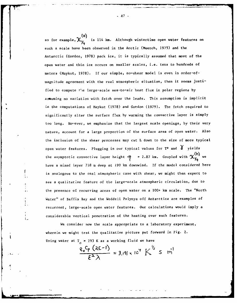
Using water at T = 293 K as a working fluid we have

*. = 3.19 II& q1,4

- 48 -

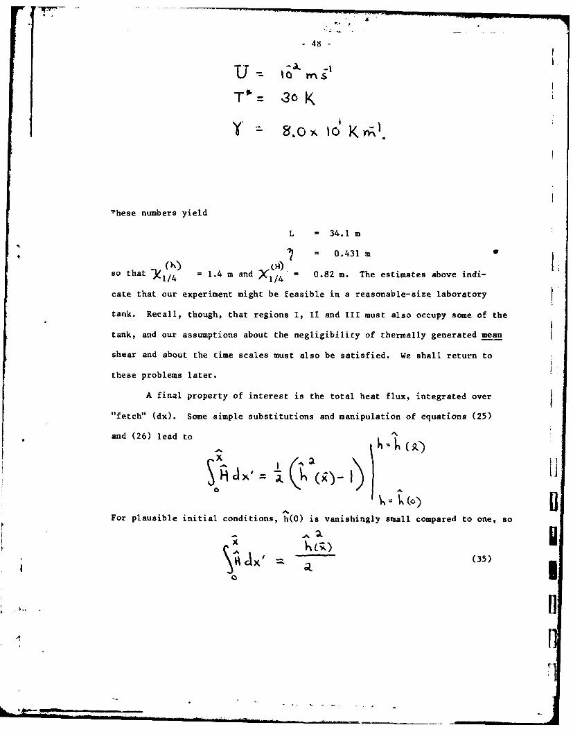
T*' = o K

These numbers yield

L = 34.1 m

= 0.431 m

so that =/4 1.4 m and X -/4 0.82 m. The estimates above indi-

cate that our experiment might be feasible in a reasonable-size laboratory

tank. Recall, though, that regions I, II and III must also occupy some of the

tank, and our assumptions about the negligibility of thermally generated mean

shear and about the time scales must also be satisfied. We shall return to

these problems later.

A final property of interest is the total heat flux, integrated over

"fetch" (dx). Some simple substitutions and manipulation of equations (25)

and (26) lead to

XX

For plausible initial conditions, h(O) is vanishingly small compared to one, so

Ii- (35)-.,.. !]

f

- 49 -

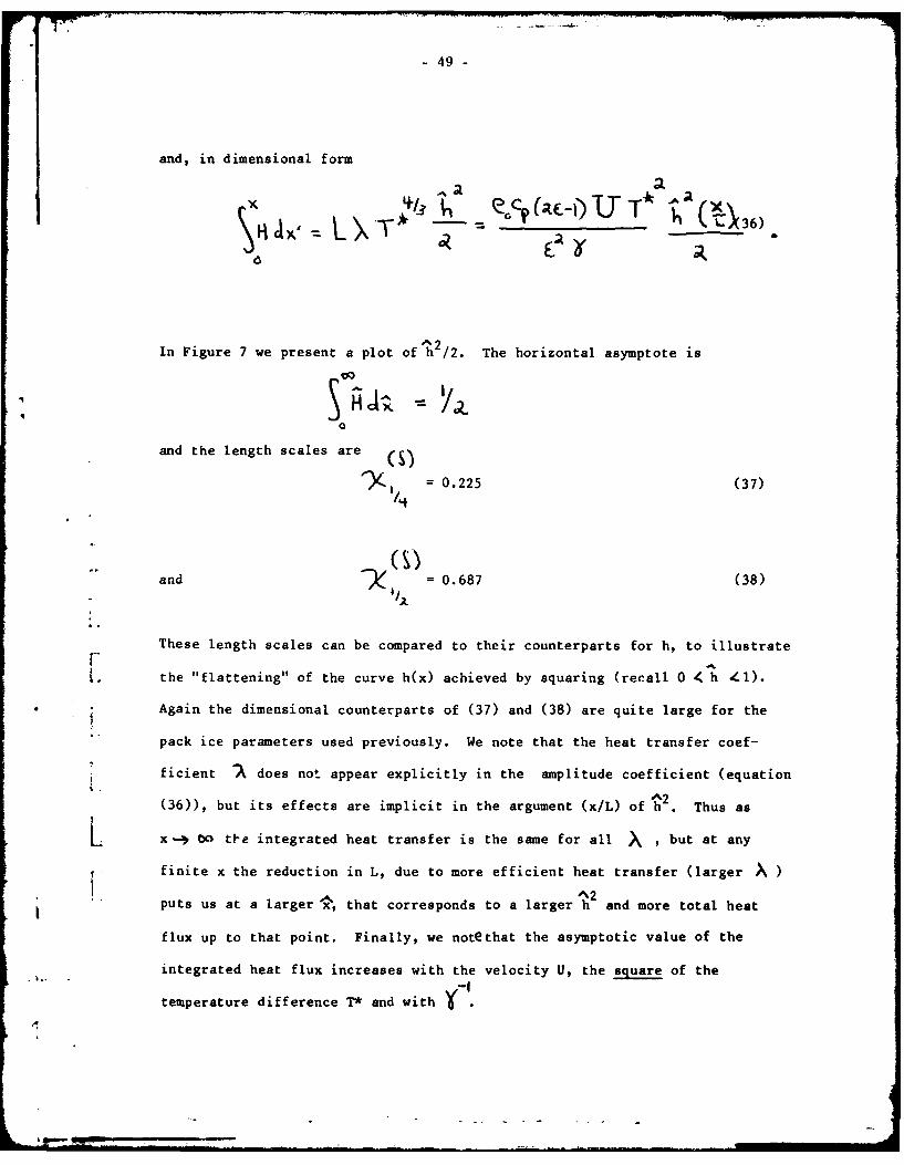
and, in dimensional form

A~ _

^2

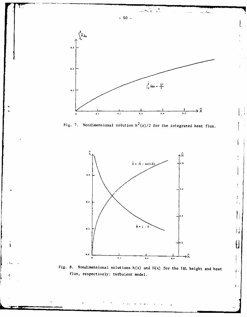
In Figure 7 we present a plot of h /2. The horizontal asymptote is

01

and the length scales are

= 0.225 (37)

(Sand - = 0.687 (38)

These length scales can be compared to their counterparts for h, to illustrate

V. the "flattening" of the curve h(x) achieved by squaring (recall 0 4 h 41).

*Again the dimensional counterparts of (37) and (38) are quite large for the

pack ice parameters used previously. We note that the heat transfer coef-

ficient A does not appear explicitly in the amplitude coefficient (equation

^2(36)), but its effects are implicit in the argument (x/L) of h . Thus as

L ~ x- 0o tfe integrated heat transfer is the same for all \ , but at any

finite x the reduction in L, due to more efficient heat transfer (larger X )

^2puts us at a larger x, that corresponds to a larger h and more total heat

flux up to that point. Finally, we notethat the asymptotic value of the

integrated heat flux increases with the velocity U, the square of the

temperature difference T* and with

50 -

0.31.

0.3

0.22

0.1

q0 0.1 0.:. O.S 0.4 O.S

Fig. 7. Nondimensional solution h (x)/2 for the integrated heat flux.

A.i

0..8

00.

0.2 I0..2

0.0 )-

00. 0.4 0.6

Fig. 8. Nondimensional solutions h(x) and 11(x) for the IBL height and heatflux, respectively: turbulent model.

-51 -

VII. Observations of the Heat Flux from Open Water

Measurements of the type needed for a reasonably complete description

of the IBL over open water in the midst of ice are non-existent (to the best

of our knowledge). Ideally we would like transects of the IBL height h(x),

the surface layer heat flux (measure via eddy correlation techniques) H(x)

Poc pw& , mean air temperature and wind speed profiles 8(x,z) and u(xz),

and the surface layer stress component Z(x) = 77iW, in addition to the0

external parameters U, T 1 and * The logistical problems associated with

* this desideratum are staggering, particularly in view of the long fetches

necessary to obtain meaningful differences in the downwind direction. Some

IBL properties over small leads (tens of meters) are reported by Andreas, et

al. (1979). Briefly, their data include calculations of the average heat flux

over 6 to 20 m wide leads, with T* in the range 23 K to 30 K. The wind speeds

u at z = 2 m vary from 2 to 4.5 m s- in the cases reported. The heat

fluxes are based on a simple conservation of energy argument, utilizing upwind

and downwind lr(z) and 0(z) profiles to compute the sea-air exchange over the

lead as a residual, and are therefore independent of assumptions about the

nature of the turbulent energy transfer over the lead. The upwind stability

is described as "stable" or "unstable" in each case. These data show a

significant positive relationship between H and S, such that the heat flux

-2 -2 --increases from 189 W m to 370 W m as u goes from 2.2 m s to

3.4 m s- and T* decreases from about 30 K to about 25 K. Our model, of

course, makes no allowance for the effects of shear embodied in G, and H.T4/3. -2

varies as T* . For T* = 30 K at x = 0 our model gives H = 103 W m

compared to about 400 W m- 2 from Andreas, et al. and over 500 W m

- 2

* .

S -

52

calculated by Maykut (1978). These last values were computed using a turbu-

lent transfer coefficient and the same ; and T* as assumed above. Surprising-

ly our simple, no-shear model gives the same order of magnitude for the flux.

On the other hand, we fear that our estimates for L and I may be seriously

in error due to our choice for the coefficieint . We make a brief digres-

sion here to pursue some of the gross differences between the "4/3-law" and a

turbulent transfer formulation for the flux.

If we assume that the turbulent IBL has adjusted to the temperature

step in a shallow surface layer, then we can apply simple empirical formulas

for steady, homogeneous shear turbulence. According to Deardorff (1968) the

turbulent heat flux can be calculated from

C C ( 7,)(39)

where the wind speed 7 and transfer coefficient CH apply at a given heightH!

z. Deardorff uses "bulk" (i.e. finite difference) stability parameters to

compute the ratio CH/CN as a function of C and the bulk Richardson

number -O( T

~.. (40)

where CHN is the transfer coefficient for neutral stability. When the

surface layer is neutral, it is useful to assume that the same eddy mechanisms Utransport heat and momentum, so that CHN C DN and CDN is a neutral

drag coefficient. Deacon and Webb (1962) present an approximate formula for

CDN over ocean surfaces

CDN (a + a2 ) (41) bri

- 53 -

where a 1 = 10- 3

=- -1

a2 7 x s0- 5 a m

If we assume a reference height z = 10 m where u f U f 5 m s and T -

T If= -20K, we have CDN = CHN = 1.35 x 10- 3 (from (41)) and RiB =

-0.27. Deardorff's calculations then give CH/CHN = 1.7, so we get CH

2.3 x 10- 3. We define AT = eocCH as a turbulent transfer coef-

ficient. In the case under consideration, X T = 2.88 J m- 3 K - . If we

retain all of the assumptions made in our earlier model, except that now we

allow the fluid to move at speed U, and carry through the analysis just as

before, using H( 6 ) = TU(TI - T ), we have

(42)

The nondimensionalization is achieved using the same as before and the

new turbulent length scale

LT J*TLr- -(43)

Equation (42) integrates to

XCh) =-(h + nlb)(44)1.

in nondimensional form. This solution is similar to the one obtained by

Fleagle and Businger (1963, p. 206), using a somewhat different approach. The

graph of (44) is shown in Fig. 8, along with the nondimensional heat flux

H(H fi - h (45)

.4

-54-

The length scales in this problem are

= 0.038

(k)

0.038

9/ = 0.193

where again we have h = T = Al in nondimensional form. The length scale (43)

may be compared with (22) for the no-shear problem. The most obvious differ-

ence is the disappearance of U. This is a result of the heat flux equation

(39), that varies directly with U. This proportionality just offsets increases

in the cold air input rate with increased heat transfer, and is a clear-cut

difference between the no-shear case and the shearing case. Also apparent is

the linear factor T* in (43) compared to T*2 /3 in (22). The linear tempera-

ture-dependence requires a longer length L to deepen the convective layer to a

given height, other factors being equal. Other factors are not equal, however,

which fact brings us to "hT* The surface heat transfer is much more effi-

cient in the turbulent case, i.e. XTU o.-3- . We can see this by

plugging in our T* and from the earlier estimate (L f 4769 kcm), to get

icLT - 1066 Km

r

so that

. i .038 --> X1/4 41 Km

.03 --- 41 .x1/4

-55-

The length scales are substantially closer to the typical extent of open water

areas. Also the heat flux ;k TUT* - 360 Wt m- 2 is in better agreement with

the objective measurements of Andreas, et al., at least for this particular

Richardson number. We are still far from the 10 to 100 m scale suggested by

Maykut for typical leads, but the simple turbulent model points quite strongly

to the importance of air mass modification cutting down the heat flux over the

larger open water features. For example, at 200 km downwind from the ice-water

edge, our heat flux would be cut by half. Gordon (1978) notes that the Weddell

Polynya can have horizontal dimensions of 200 km x 500 km at certain times.

In this case, the assumption of heat flux constant with fetch would be incor-

rect, according to our calculations. We note, however, that we have kept the

Richardson number constant, when, in fact, as the air warms Ri is reduced,

thus reducing the heat flux from our earlier estimate. This simply reinforces

our conclusion, because it implies, for the complete heat flux, a higher power

than T*1 and a larger A T than . However, L T will be a little larger

than we calculated above. It seems that the simple, no-shear model can provide

us with some qualitative insight into the nature of the parameters that deter-

mine the IBL properties. The flux and length scales are correct to order of

magnitude, but incorporation of the shear effects is necessary to bring the

scales into more quantitative agreement with measurements. Also, the dif-

ference in length scales is such that the inclusion of shear just brings the

modification of the heat flux to the status of an "important" parameter, due

to the scales of open water found in nature.

VIII. Scale Analysis of Some Processes in the No-shear Model

In this section we just briefly mention some rough measures of the

validity of our picture (Fig. 2), given typical parameters. Our primary

-56-

assumptions are

1) T is constant on 5 < Z <m

2) j& T is a step change in temperature

3)H(6 ) (T T 4/3

4) Steady conditions prevail with respect to the coordinate X . j0

We shall not treat (1) and (2) here, but simply reiterate that they are

consistent with observations, and the results are not sensitive to (2). Our

third assumption is valid if shear turbulence is not generated and the time

scale for individual thermals t* is much less than m , the scale for a

small (say 5%) change in T . If this last is satisfied then we can suc-m

cessfully exploit the averaging operator (page 6) by sandwiching its time

scale T between t* and t'"m. We intuitively expect (4) to hold, but a

laboratory experiment is needed to verify this.

Let's look at assumption (3). To avoid shear effects we would hope to

minimize mean horizontal circulations, because our fluids are viscous and

bounded by a solid plate. In the case of uniform heating from below

(e.g. U-0,o) there is no tendency to generate mean horizontal pressure

gradients. ft

However, we have horizontal variations in 6 on level surfaces,

indicating that pressure gradients will form in regions I through IV. In

region IV we already have seen that L is large, and the horizontal pressure

gradients induced by the heating will vary as L -. Furthermore, the thermal

turbulence should produce an extremely large "mixing length" for momentum, ,

because thermals near the plate have effectively zero ;-moment,- and rise all

the way up to z - h. The horizontal circulations in IV might, then, be

acceptably small, but this problem requires further work.

.., . - .. . . . .4. -. . . . . . . . . . . . .... . ., .. . . . . , . . .. . . , . ,,

57 -

In regions I and II we would like molecular diffusion to build up the

thermal boundary layer so that it can rapidly convect. Hopefully this would

occur before the thermally-generated mean flow develops substantially,

although we still might expect eventual thermal plumes even if the boundary

layer were disrupted by shear for small x'. For order-of-magnitude purposes,

we introduce a boundary layer

depth (46)

9

characteristic of thermal diffusion. If the "critical" Rayleigh number for

this layer is about 1500 (Howard, 1964) then S , the critical depth is

In the following computations we choose the nominal values for air: T* = 25K,

10 f 2 km- 1 U = 5 ins 1 and for water (in the lab): T* =30 =

80 1 U = 10 -ms

From these values we have, for air

0.8cm

t* I sec

X*= 5m

and for water

SS 0.2 cm

t. --, sec

X* -% 5 cm

Notice that X* is quite acceptable for a laboratory tank roughly 2 m long.

Qualitatively, Heidt's (1977) h(t) data for uniform heating indicate a length

of less than 10 cm for region III, assuming t = X'/TJ , so, in principle, we

could see more than I m of region IV in a 2 m tank. Now, just ahead of region

-58-

I, the fluid is at rest. If we linearize the 2-D Boussinesq vorticity

equation about u - w o, we have

-- 3L-ay, (47)

where = - is the vorticity. If the temperature gradient is

assumed known from molecular diffusion and is set to zero, we will

have just enough vorticity so that viscosity balances the pressure gradient.

Because a finite time is required for the fluid to obtain this vorticity,

and " would be smoothed out by the motion, 5 estimated this way should

be larger than the value that occurs. If we assume a linear temperature

gradient in the vertical T*/6 where = , than we get

We scale the vorticity dissipation as

aa Z3

Our hypothetical balance requires

a o =T T '

Where Or is the Prandtl number. Region II ends where so our nominal3x0 - 3 for airand 3 -1

values give us 3x -e-1= for air and a m

for water. These numbers are overestimates, and indicate the insignificance of

.-.

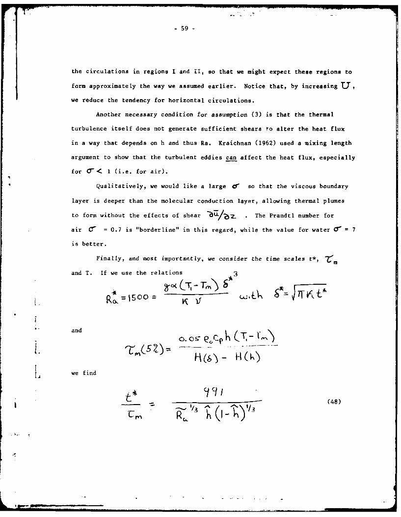
59 -

the circulations in regions I and iI, so that we might expect these regions to

form approximately the way we assumed earlier. Notice that, by increasing U,we reduce the tendency for horizontal circulations.

Another necessary condition for assumption (3) is that the thermal

turbulence itself does not generate sufficient shears to alter the heat flux

in a way that depends on h and thus Ra. Kraichnan (1962) used a mixing length

argument to show that the turbulent eddies can affect the heat flux, especially

for Cr < 1 (i.e. for air).

Qualitatively, we would like a large e so that the viscous boundary

layer is deeper than the molecular conduction layer, allowing thermal plumes

to form without the effects of shear . The Prandtl number for

air C' = 0.7 is "borderline" in this regard, while the value for water = 7

is better.

Finally, and most importantly, we consider the time scales t*, 7'

and T. If we use the relations

and 0(C(T, ( N )

wend

i .O .. ..

~we find

-"- -(48)

Cv1/3R ..

60 -

where

Thus t*/-. m should be small to guarantee the existence of a T for valid

averaging.

This ratio decreases as h increases, and we useh = 0.1 along with our

nominal , * and J values to obtain

t* =2.5 x 10-

1

for air, and

t* = 3.15

for water. Thus we have about 400 thermals in the time needed for T - T

to change by 5% in air at h = 0.1. This seems sufficient. However, the water

case looks quite bad, and we might expect the 4/3 law not to apply to pene-

trative convection wherein Tm is not constant with time. We hope to assess

the data of Heidt (1977) in future work to see if his heat fluxes follow a 4/3

power law.

IX. Conclusion

We have constructed simple models of IBL properties and investigated

the resulting scales as they depend on T*, U and f . For the pure

*. convective case (no-shear) the "fetch" scales are quite long for air.

- 61 -

However, a simple shear-turbulence model indicates that heat fluxes may vary

significantly with fetch over the larger open water areas of the polar

oceans. The analyses of a possible laboratory simulation of the convective

model indicate problems with the 4/3 law. We hope to pursue this in future

work. Also, the linearized vorticity and heat equations can be solved for an

imposed surface temperature step at Xo, eliminating the need for scaling

arguments in regions I and II.

Acknowledgements

I would like to thank the entire GFD Staff, and Dr. Melvin Stern in

particular, for their constructive advice and encouragement this summer.

REFERENCES

Andreas, E. L., C. A. Paulson, R. M. Williams, A. W. Lindsay and J. A.Businger, 1979. The turbulent heat flux from Arctic leads. BoundaryLayer Meteorology (in press).

Carson, D. J. and F. B. Smith, 1974. Thermodynamic model for the developmentof a convectively unstable boundary layer. Advances in Geophysics,18A, 111-124.

Deacon, E. L. and E. K. Webb, 1962. Small-scale interactions. The Sea,New York, Interscience, 43-87.

Deardorff, J. W. 1968. Dependence of air-sea transfer coefficients on bulkability. Jour. Geophys. Res., 73, 2549-2557.

Fleagle, R. G. and J. A. Businger, 1963. An Introduction to AtmosphericPhysics. New York, Academic Press, 206-207.

Gordon, A. L., 1978. Deep Antarctic convection west of Maud Rise. Jour.Phys. Oceanogr., 8, 600-612.

Gordon, A. L., 1979. Meridional heat and salt fluxes in the Southern Ocean.

WHOI GFD Lecture.

Heidt, F. D., 1977. The growth of the mixed layer in a stratified fluid due

to penetrative convection. Boundary Layer Meteorology, 12, 439-461.

Howard, L. N., 1964. Convection at high Rayleigh number. Proc. llth Inter.Congress of Appl. Mechanics, Berlin, Springer-Verlag, 1109-1115.

L k , - _ , . .

62- L.

Kraichnan, R. H., 1962. Turbulent thermal convection at arbitrary Prandtl

number. Physics of Fluids, 5, 1374-1389.

Lenschow, D. H., 1974. Model of the height variation of the turbulencekinetic energy budget in the unstable planetary boundary layer. J.Atmos. Sci., 31, 465-474.

Maykut, G. A., 1978. Energy exchange over young sea ice in the centralArctic. Jour. Geophys. Res., 83, 3646-3658.

Plate, E. J., 1971. Aerodynamic characteristics of atmospheric boundarylayers. U. S. Atomic Energy Commission, Oak Ridge.

Roisin, B., 1979. Penetrative convection. WHOI GFD Lecture.

Stern, M. E., 1975. Ocean Circulation Physics. Academic Press,New York, 181-183.

Townsend, A. A., 1959. Temperature fluctuations over a heated horizontal

surface. Jour. Fluid Mech., 5, 209-241.

Turner, J. S., 1973. Buoyancy effects in fluids. Univ. Press, Cambridge,U.K., 367 pp.

Willis, G. E. and J. W. Deardorff, 1974. A laboratory model of the unstableplanetary boundary layer. Jour. Atmos. Sci., 31, 1297-1307.

L

Ii

- 63 -

A LABORATORY MODEL OF CHIMNEY INSTABILITY

Thomas Keffer

I. The Physical Problem

One might ask why the ocean would choose such a complicated process as

chimneying to release its heat to the atmosphere. Why not just simple con-

vection or the deepening of a mixed layer? The answer is that, in general,

the ocean does not lose much heat via the relatively rare process of chim-

neying. But the resulting water products are often dramatically different

from surrounding waters and hence attract much attention. Relatively large

quantities of dense water can be created in the mid-ocean and moved to the bot-

tom in an organized manner without losing its characteristics to surrounding

waters.

II. Observational Background

Chimneying has been observed or suspected to occur in four areas. Of

these, the Gulf of Lions in the northwest Mediterranean is by far the most

intensively studied. It has been the subject of studies by the MEDOC group in

1979, 1975, and 1970. The consensus from these studies is that chimneying

occurs in three distinct phases (at least in the Mediterranean) (Killworth,

1979):

1) Preconditioning:

This stage is characterized by a doming of the isopycnals in a small (1200

km2 ) area of the ocean (Fig. 1), geostrophically balanced by a surrounding

cyclonic circulation. The static stability is much reduced in the center of

the dome from values a small distance away. The exact causes of precon-

ditioning are unknown but, in the case of the Gulf of Lions, topographic

constraints are suspected (Hogg, 1973).

ow-

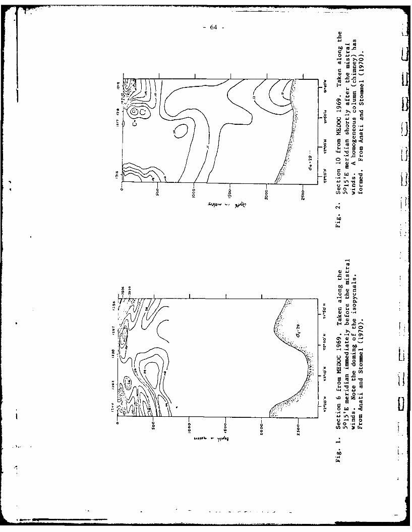
-64 -

00 C.

Cu4 to>%09.

CO C- -

04"

* C 0 03

1001

*.4 COO

07 -).4 0

-4C

-na)

0 0

0 ) '0 J-4-0

-4 4 C 0 % L04)

0 6

4-400

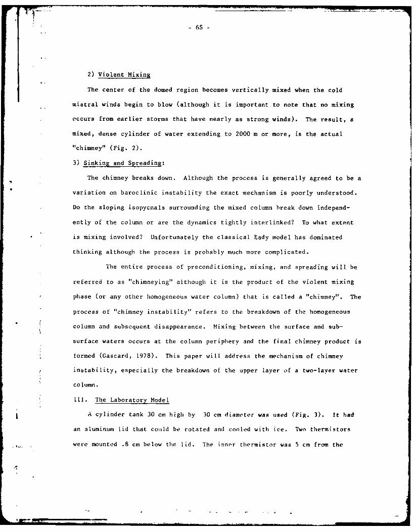
65 -

2) Violent Mixing

The center of the domed region becomes vertically mixed when the cold

mistral winds begin to blow (although it is important to note that no mixing

occurs from earlier storms that have nearly as strong winds). The result, a

mixed, dense cylinder of water extending to 2000 m or more, is the actual

"chimney" (Fig. 2).

3) Sinking and Spreading:

The chimney breaks down. Although the process is generally agreed to be a

variation on baroclinic instability the exact mechanism is poorly understood.

Do the sloping isopycnals surrounding the mixed column break down independ-

ently of the column or are the dynamics tightly interlinked? To what extent

is mixing involved? Unfortunately the classical Eady model has dominated

thinking although the process is probably much more complicated.

The entire process of preconditioning, mixing, and spreading will be

referred to as "chimneying" although it is the product of the violent mixing

phase (or any other homogeneous water column) that is called a "chimney". The

process of "chimney instability" refers to the breakdown of the homogeneous

column and subsequent disappearance. Mixing between the surface and sub-

surface waters occurs at the column periphery and the final chimney product is

formed (Gascard, L978). This paper will address the mechanism of chimney

instability, especially the breakdown of the upper layer of a two-layer water

column.

Ill. The Laboratory Model

A cylinder tank 30 cm high by 30 cm diameter was used (Fig. 3). It had

an aluminum Lid that could be rotated and cooled with ice. Two thermistors

were mounted .8 cm below the lid. The inner thermistor was 5 cm from the

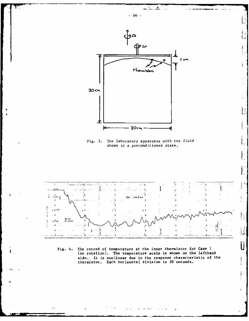
-66-

30 C-%

Fig. 3. The laboratory apparatus with the fluid7

shown in a preconditioned state. L

1, /VSI - I. .

.. . . .. .. . . . . . . . .. . . . .- 4. . . . . . . . .. . . . . . . . . . . . . . . .. . . . . . . . .t ' $. . .. . . . . . . . . . . . .I ,

Fig 4. Th eodo eprtr tte ie ----------- rCas a1

(n rottin) Th eprtr cl s hw ntelfhn

sie It is nolna du to th repos chrceitco h

thrmstr Eahhrznaldvso s.0scns

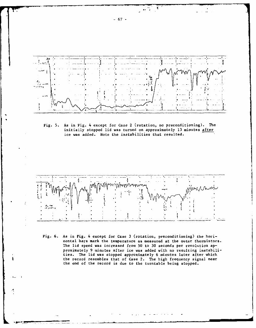
- 67 -

I I '

- • +.. .. . .. .. . .. . .. .-... .. . ' -. -.. .. .. . .. . .. .. . .. .. . ...... . . .... ... .... ...

I7.

Fig. 5. As in Fig. 4 except for Case 2 (rotation, no preconditioning). Theinitially stopped lid was turned on approximately 13 minutes after

ice was added. Note the instabilities that resulted.

. ... . .... .......... . .......... ....... ............................................

.! .. u . ...... . ... .... .. _1.... ....t _ _..J. ... .... .................. ..J+_ .....-L

Fig. 6. As in Fig. 4 except for Case 3 (rotation, preconditioning) . he

ntiall sTope lid was ppedo approximately 13 minutes afterhcthe recor ree.bNoe that ofnsbles That hg reuenc. gana

........................ ............. .i.

Fig. 6. As in Fig. 4 except for Case 3 (rotation, preconditioning) the hori-zontal bars mark the temperature as measured at the outer thermistors.The lid speed was increased from 50 to 30 seconds per revolution ap-proximately 9 minutes after ice was added with no resulting intabili-ties. The lid was stopped approximately 6 minutes later after whichthe record resembles that of Case 2. The high frequency signal nearthe end of the record is due to the turntable being stopped.

.,.

A!

q iii

Fig. 7. A typical picture for Case 2 (rotation, no preconditioning) using adyed upper layer (taken approximately 10 minutes after ice was added).Note the columns below the interface with length scale of approxi-mately the Rossby radius of deformation (2 cm).

Fig. 8. A typical picture for Case 3 (rotation, preconditioning) usingfluoroscein dye in the upper layer, taken 3 minutes after ice wasadded. Long, growing columns extend into the interior of the lowerlayer. Within 10 minutes the entire lower layer was filled with

S..dye.

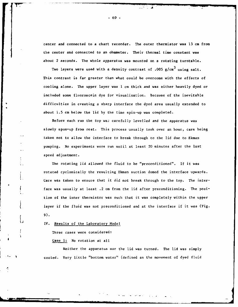
- 69 -

center and connected to a chart recorder. The outer thermistor was 13 cm from

the center and connected to an ohmmeter. Their thermal time constant was

about 2 seconds. The whole apparatus was mounted on a rotating turntable.

Two layers were used with a density contrast of .005 g/cm 3 using salt.

This contrast is far greater than what could be overcome with the effects of

cooling alone. The upper layer was 1 cm thick and was either heavily dyed or

included some fluoroscein dye for visualization. Because of the inevitable

difficulties in creating a sharp interface the dyed area usually extended to

about 1.5 cm below the lid by the time spin-up was completed.

Before each run the top waz carefully levelled and the apparatus was

slowly spun-up from rest. This process usually took over an hour, care being

taken not to allow the interface to break through to the lid due to Ekman

pumping. No experiments were run until at least 20 minutes after the last

speed adjustment.

The rotating lid allowed the fluid to be "preconditioned". If it was

rotated cyclonically the resulting Ekman suction domed the interface upwards.

Care was taken to ensure that it did not break through to the top. The inter-

face was usually at least .2 cm from the lid after preconditioning. The posi-

tion of the inner thermistor was such that it was completely within the upper

i layer if the fluid was not preconditioned and at the interface if it was (Fig.

9).

IV. Results of the Laboratory Model

Three cases were considered:

Case 1: No rotation at all

Neither the apparatus nor the lid was turned. The lid was simply

cooled. Very little "bottom water" (defined as the movement of dyed fluid

L" = '' . . " i ... . . ' l - ' . . . ' .. . .. . .

rJ

70 -

downward into the interior) was produced. Time scales as seen by the inner

thermistor were very long (Fig. 4). What production there was seemed to be due

to mixing at the interface where enough salt could be mixed in to allow the

fluid to sink. No signs of the formation of double diffusive interfaces could

be seen within the short time it was watched (30 minutes).

Case 2: Rotation but no Preconditioning.

There was, again, very little bottom water production. Time scales

were long and temperature perturbations, as measured by the inner thermistor,

were small (Fig. 5). Small bulges (Fig. 7) with a scale on the order of the

Rossby radius (2 cm) could be seen on the interface. The inner thermistor was

4-8 0C colder than the outer thermistor, probably due to their relative dis-

tance from the cylinder's edge.

Case 3: Rotation and Preconditioning

The fluid was preconditioned before ice was added. The resulting tem-

perature record at the inner thermistor can be seen in Fig. 6. Large tempera-

ture fluctuations (100 C) with short time scales (10-15 seconds per spike)

can be seen. There was extensive bottom water production (Fig. 8). Close

analysiL of movies taken immediately after ice was added showed that insta-

bilities of the interface started at about 5 cm from the center of the cylinder

and "grew into" the thicker parts of the upper layer. The preconditioned

interface was thin, but still sloping, at the preferred starting point.

The observations suggest a structure as in Fig 9. The interface was

originally dome shaped and then developed small, wavelike, azimuthal,

perturbations that rapidly grew until they produced long columns as in Fig. 8.

The thermistor record can be explained as follows: When the interface was

high the thermistor was exposed to the warm water of the lower layer. When

.- 1

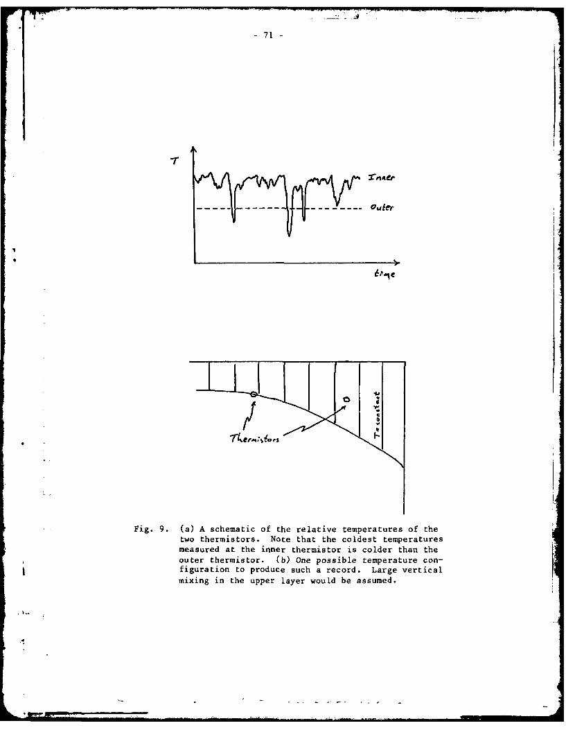
- 71!

"I

1

Fig. 9. (a) A schematic of the relative temperatures of thetwo thermistors. Note that the coldest temperaturesmeasured at the inner thermistor is colder than theouter thermistor. (b) One possible temperature con-figuration to produce such a record. Large verticalmixing in the upper layer would be assumed.

-72-

the interface moved down the thermistor felt the cold water of the upper layer

but it was even colder than the water at the outer thermistor. The difference

of 3-60C represents a density difference of about 5x1_ 4 g/cm 3 or one-

tenth of the density contrast between the two layers. This small density

gradient in the upper layer can be extremely destabilizing as will be shown in

Section 6.

In the lab experiment the density gradient could be created by any of

the three different mechanisms. First, of course, is the relative distance jfrom the edge of the cylinder. The effects of this were seen in Case 2.

Second, for a constant heat flux thinner parts of the upper layer will become

colder than the thicker parts. Finally, if mixing with the lower layer were -

to occur it will happen at the thinnest parts of the upper layer first. The

mixed in salt would increase the density at the center relative to the edges.

In the ocean, the last two mechanisms could operate and suggest looking care-

fully for correlations in changes of radial density gradients with subsequent

chimney breakdown.

It is worth noting that if the fluid is "preconditioned" after ice is

added the resulting action resembles Case 3 very closely. This was done with

the run showed in Fig. 5. Hence, a cooled fluid can be "postconditioned" and

still result in chimney instability. This may be difficult to do in the ocean

due to the long time scale usually associated with doming of the interface.

V. Theoretical Model14

A theoretical model is developed using a rotating annulus of width L with

rigid lid containing a two-layer fluid of density contrast

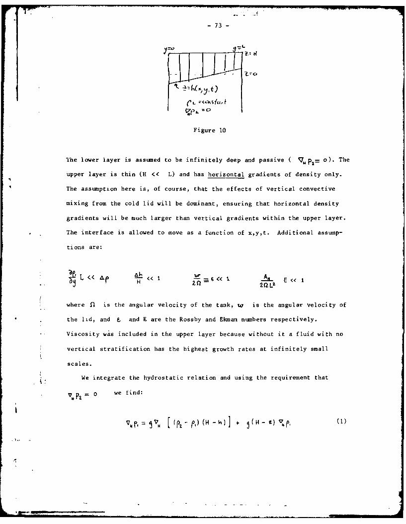
- 73 -

y, = .o' ,, -

Figure 10

The lower layer is assumed to be infinitely deep and passive ( o 0). The

upper layer is thin (H << L) and has horizontal gradients of density only.

The assumption here is, of course, that the effects of vertical convective

mixing from the cold lid will be dominant, ensuring that horizontal density

gradients will be much larger than vertical gradients within the upper layer.

The interface is allowed to move as a function of x,y,t. Additional assump-

tions are:

L< << &- << - E < 1H - 2 <L1

where fl is the angular velocity of the tank, ur is the angular velocity of

the lid, and & and E are the Rossby and Ekman numbers respectively.

• Viscosity was included in the upper layer because without it a fluid with no

vertical stratification has the highest growth rates at infinitely small

scales.

We integrate the hydrostatic relation and using the requirement that

V t 2 o we find:

,V

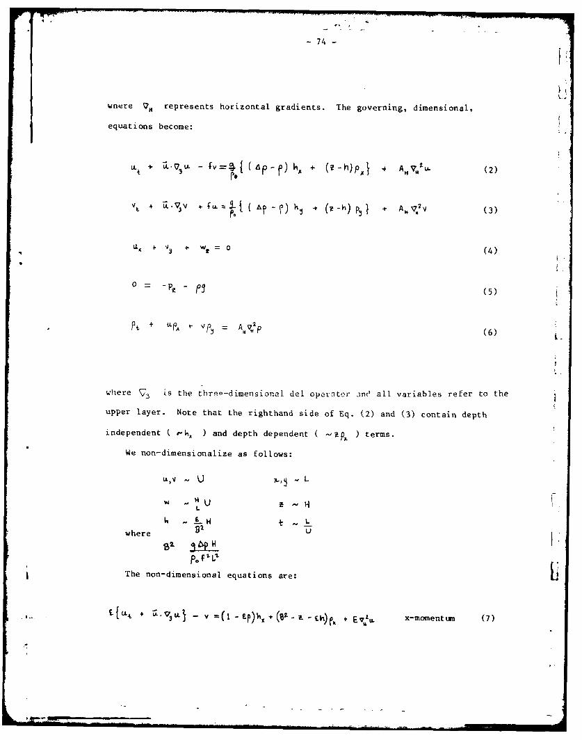
- 74 -

wnere V. represents horizontal gradients. The governing, dimensional,

equations become:

LL t + Lk LA.e ' )hA + (.~p P 1 A IVOU (2)

,,V t~ ,, M :[. V3-I) v, L,_ p } + A. V. (3)

LI + V + w 0 (4)

0 = -p - (5)

+ 'PA~ V~ A49p (6)

where V. is the threF-dimensional del operator anO all variables refer to the

upper layer. Note that the righthand side of Eq. (2) and (3) contain depth

independent ( k, ) and depth dependent ( ,p, ) terms.

We non-dimensionalize as follows:

W 4U Hw HU •,,L

6 L .H .tL

where 91

. f ;po f1L" LThe non-dimensional equations are:

. . - v - ' -f h) Eu. x-momentum (7)

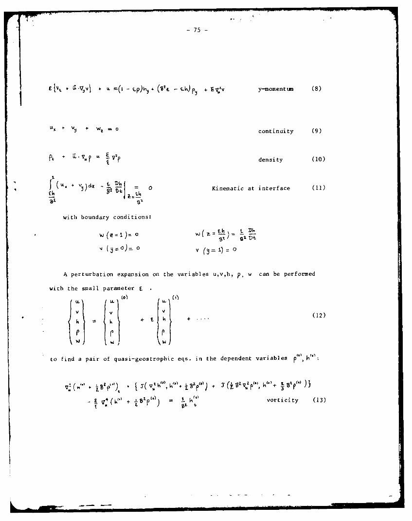
- 75 -

C. --VA +,t ( PE -).') (1;2 E; y-momentum (8)

LA A 3 * w = o continuity (9)

Pt + UVVO density (10)

+ _ 0 Kinematic at interface (ii)

with boundary conditions:

( =o)V 0 L) (= = o

A perturbation expansion on the variables u,v,h, p, w can be performed

with the small parameter F-

(0)

V V v (2S + +(12)

~W

to find a pair of quasi-geostrophic eqs. in the dependent variables p ,

L B ' I k °01vorticity (13)B&

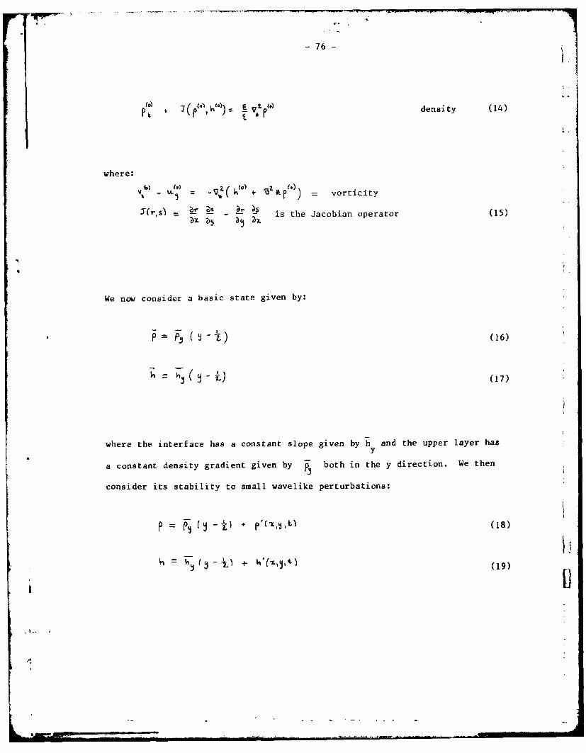
-76-

) -= WO) density (14)

a.

where:

V ( (o) 4- B = vorticity

Y(rss _ v- D S is the Jacobian operator (15)

We now consider a basic state given by:

where the interface has a constant slope given by h and the upper layer hasY

a constant density gradient given by T both in the y direction. We then

consider its stability to small wavelike perturbations:

p = t)--i) ' (18)

+4

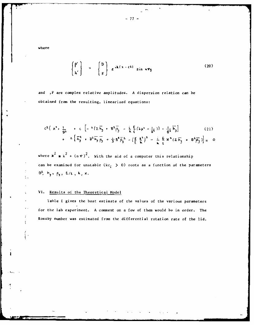
- 77 -

where

fCI X ( t)Si}n (20)

and ,F are complex relative amplitudes. A dispersion relation can be

obtained from the resulting, linearized equations:

( K'- + C ... (21)

2 2 2where - k + (nir) With the aid of a computer this relationship

can be examined for unstable (kc. > 0) roots as a function of the parameters

: 1 I , p , EI. k .

VI. Results of the Theoretical Model

Table I gives the best estimate of the values of the various parameters

for the lab experiment. A comment on a few of them would be in order. The

Rossby number was estimated from the differential rotation rate of the lid.

b[ ."

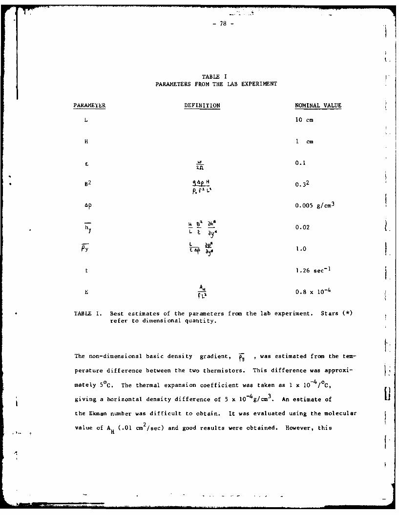
-78-

t.

TABLE IPARAMETERS FROM THE LAB EXPERIMENT

PARAMETER DEFINITION NOMINAL VALUE

L 10 cm

H 1cm

! 0.1

• B2 0.32

4P p 0.005 g/cm3141

L -0.02L t. ,

1 0L ,VY E&P5 % 1.0

1.26 sec - 1

tI

E 0.8 x 10 - 4

TABLE I. Best estimates of the parameters from the lab experiment. Stars (*)refer to dimensional quantity.

The non-dimensional basic density gradient, , was estimated from the tem-

perature difference between the two thermistors. This difference was approxi-

mately 50C. The thermal expansion coefficient was taken as I x 10-4 / C,

giving a horizontal density difference of 5 x 10-4 g/cm 3 . An estimate of

the Ekman number was difficult to obtain. It was evaluated using the molecular

value of AH (.01 cm2/sec) and good results were obtained. However, this

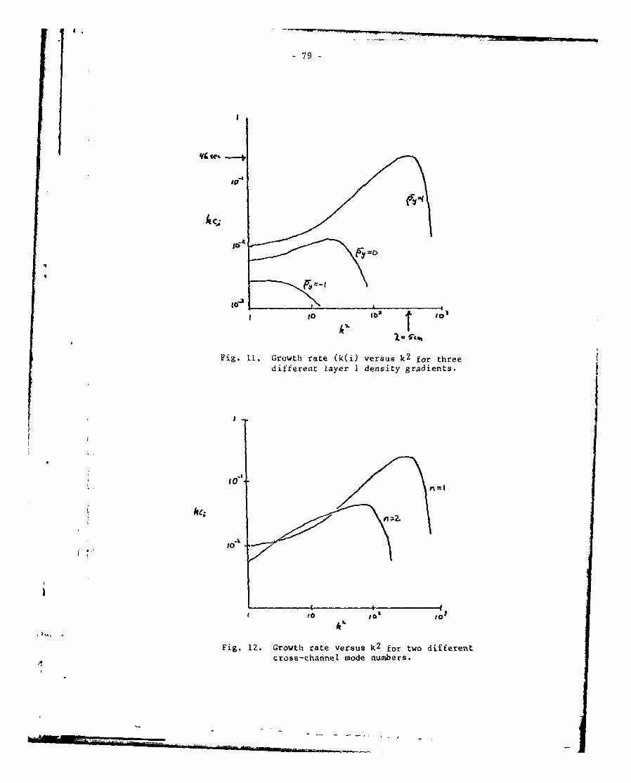
47

-79-

to

Fig. 12. Growth rate ()versus k2 for tdifretdcfros n-chane 1ode nimyer. ens

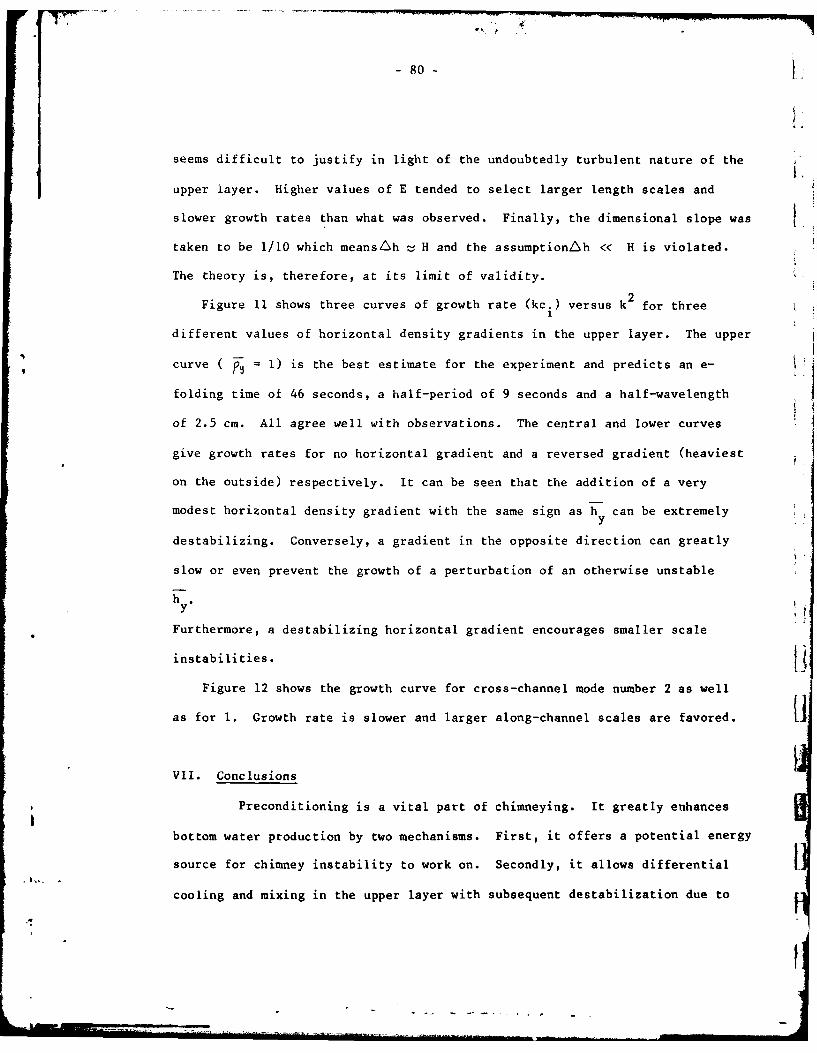
-80-

seems difficult to justify in light of the undoubtedly turbulent nature of the

upper layer. Higher values of E tended to select larger length scales and

slower growth rates than what was observed. Finally, the dimensional slope was

taken to be 1/10 which meansLh z, H and the assumptionZh << H is violated.

The theory is, therefore, at its limit of validity.

Figure 11 shows three curves of growth rate (kc.) versus k 2for three

different values of horizontal density gradients in the upper layer. The upper

curve P4 p 1) is the best estimate for the experiment and predicts an e-

folding time oi 46 seconds, a half-period of 9 seconds and a half-wavelength

of 2.5 cm. All agree well with observations. The central and lower curves

give growth rates for no horizontal gradient and a reversed gradient (heaviest

on the outside) respectively. It can be seen that the addition of a very

modest horizontal density gradient with the same sign as h ycan be extremely

destabilizing. Conversely, a gradient in the opposite direction can greatly

slow or even prevent the growth of a perturbation of an otherwise unstable

h.* y*

Furthermore, a destabilizing horizontal gradient encourages smaller scale

instabilities. 1Figure 12 shows the growth curve for cross-channel mode number 2 as well

as for 1. Growth rate is slower and larger along-channel scales are favored. i

VII. Conclusions

Preconditioning is a vital part of chimneying. It greatly enhances

bottom water production by two mechanisms. First, it offers a potential energy

source for chimney instability to work on. Secondly, it allows differential

cooling and mixing in the upper layer with subsequent destabilization due to

-81-

the resulting horizontal gradients. What is not known is the role of the homo-

geneous column as an energy source. A follow up study should address the dy-

namics of this central column.

Instabilities seem to start on the slopes of the thinnest parts of the

upper layer and "grow into" the thicker parts. This may be due to the largest

horizontal density gradients being created here by nearby mixing. As the in-

stabilities grow they may mix in dense fluid, moving the density gradient out-

wards, and the instabilities follow.

Finally, the fastest growing wavelengths are not necessarily of theI

order of the Rossby radius of deformation. The theoretical analysis indicates

that the horizontal scale may be set by friction and the magnitude of the

layer 1 horizontal density gradients.

VIII Acknowledgments

Special thanks are due to Peter Killworth and John Whitehead for their

guidance and assistance. Many thanks is also owed to Robert Frazel for his

helpful technical assistance.

REFERENCES

Anati, D. and H. Stommel, 1970. The initial phase of deep-water formation inthe Northwest Mediterranean, during MEDOC, 1969. CabiersOceanographiques, 22, 347-351.

Gascard, J. C., 1978. Mediterranean deep water formation, baroclinic insta-bility and oceanic eddies. Oceanologica Acta, 1(3), 315-330.

Hogg, N. G., 1973. The preconditioning phase of MEDOC 1969. I. Topographiceffects. Deep-Sea Res., 20, 449-459.

(Killworth, P. D., 1979. On chimney formations in the ocean. J. Phys.Oceanogr., 9, 531-554.

* .

4.

-82-

A MODEL FOR THE SEASONAL VARIATION OF

THE MIXED LAYER IN THE ARCTIC OCEAN

PETER LEMKE

1. Introduction

Models bor the oceanic mixed layer are of special importance in climate

related problems, since the mixed layer represents the link between the

atmosphere and the interior ocean.

There are a variety of models that describe the time evolution of the

mixed layer pi-operties in the open oceans, where wind mixing and seasonal

varying heating and cooling are the dominant forcing mechanisms that form the

mixed layer. For a review see Niiler and Kraus (1977).

Despite the heavy ice cover a well developed mixed layer is also

ooserved in the Arctic Ocean. 'ihe dominant forcing mechanisms here are ice

melting and freezing and mechanical mixing due to keel stirring induced by the

ice motion. Observations show (McPhee, 1978; Hunkins, Bauer and Amos, 1977)1

that during most of the year the base of the mixed layer is sharply defined,j

the depth of which varies from 40-50 m in late May to 15-25 m in the sumnmer.

The salinity varies from 30.5 0/00 to 29.8 o/oo respectively.

In this paper a rough quantitative description of the observed data is

achieved from a one-dimensional mixed layer model.

iI. One-Dimensional Mixed Layer Model

One-dimensional models of the upper ocean are useful since vertical

variations of temperature and salinity are more pronounced than horizontal

changes. For many purposes the upper ocean layers can therefore be treated as

homogeneous along the horizontal, so that the horizontal derivatives can be Iomitted in the governing equations. This is especially true for the Arctic

Ucean (see Fig. 2, SCOR Report). Since temperature, salinity, density and

-83-

velocity fields interact with each other, a complete model has to describe the

evolution ot each of these properties. The prognostic equations can be

derived from a set of one-dimensional conservation equations. In particular,

the salt flux balance leads to an equation for the bulk salinity

W'6' 0_(1)

where S' S an S W' W - W are the deviations from their mean

values. Similar equations can be derived for temperature, buoyancy and hori-

zontal velocity V (Niiler and Kraus, 1977).

lo solve this set of equations one has to find explicit expressions for

the turbulent fluxes. This has been done in several ways, i.e., in turbulence

closure models, by eddy coefficient. and mixing length hypothesis and in mixed

layer models.

In the latter models it is assumed that mean temperature, salinity and

horizontal velocity are uniform in the vertical within the mixed layer. This

assumption permits vertical integration of (1) and the equivalent equations

tor temperature, buoyancy and horizontal momentum from the bottom to the top

of the mixed layer. Now these mixed layer properties are described as

functions of exchanges with the air above and the deep ocean below.

Since with the time-dependent mixed layer depth H(t) a new variable is

introduced, the system has to be closed by an equation for the entrainment

velocity w e defined by

w adH for dli > 0

w=0 for di <0e At

rT-7 --- - - PRMOIPIP

V. p.

-84-

Entrainment is associated with layer deepening. There is no

entrainment during the retreat of the mixed layer. The closure of the system

is achieved by introduction of the turbulence energy equation. This is given

in simplified form by (Niiler and Kraus, 1977).

%(0 Z V"U: 41 nHi8 +- 1 (2)6!

with c2 = H 6 b, where i/kb is the buoyancy step at the lower interface of1.y

the mixed layer, c i is the velocity of the long interval waves at the lower

interface, u, is the friction velocity, B is the buoyancy flux at the

surface and I is the rate of potential energy change produced by penetrating

solar radiation, C , m and n are parameters. The meanings of the terms are:

A: Work per unit time needed to lift the dense entrained water and to

mix it through the layer;

C: rate at which energy of the mean velocity field is reduced by mixing

across the layer base;

D: rate of working by the wind;

L: rate of potential energy change produced by fluxes across the sea

surface.

In order to complete Eq. (2) a dissipative term has to be added. But

it is assumed that this term is composed of terms which are individually

proportional to the active turbulence generating process, described by C, D

and also by b during the cooling period when B is positive.

Therefore the parameters , m and n in Eq. (2) include a Uparameterization of the dissipation (n = 1 during the heating period when

B < 0). With the turbulence energy equation (2) the set of differential

equations for the mixed layer is closed.

' '-For given fluxes at the surface and at the lower interface the

evolution of the mixed layer properties can be described. Usually mixed layer

L(

---- ----

models are applied to open ocean, where wind mixing and time varying buoyancy

flux at the surface, due to heating and cooling, determine the seasonal

variation of the mixed layer. Since the seasonal variation is more pronounced

in heating and cooling than in evaporation and precipitation the main

variables in these models are temperature and depth. The important features

of the evolution of the mixed layer described in such one-dimensional models

are:

a) a pronounced retreat of the mixed layer during the period of

increased heating,

b) a slow deepening of the mixed layer during the period of decreased

heating,

c) a faster deepening during the cooling period, due to wind mixing and

mixing through thermal convection.

III. Application to the Arctic Ocean

The one-dimensional mixed layer model described by Niiler and Kraus

(1977) is now applied to an ice covered ocean. In this case the seasonal

variation of the air temperature (heating, cooling) has nearly no effect on

the temperature of the mixed layer. Observations indicate that the mixed

layer temperature exhibits nearly no seasonal variation and is near the

freezing point down to a depth of 60 m all over the year (Hunkins, Bauer and

Amos, 1977). All net heat fluxes are used to freeze and melt ice. During ice

melting fresh water is added on top of the mixed layer that tends to stabilize

the stratification. During the freezing period brine is excluded from the

newly formed ice, a layer of dense salty w'ater destabilizes the stratification

and brine convection starts to develop.

Therefore, the seasonal variation of surface air temperature manifests

itself in a seasonal varying buoyancy flux due to positive fresh water flux in

86

summer and negative tresh water flux (out of the mixed layer) during winter-

time. Consequently, in contrast to the open ocean, the main variables in a

polar mixed layer model must be salinity and depth. For simplicity it is

assmed in this paper that the mean horizontal velocity in the mixed layer is

zero t- = U).

'Ihere are two principal stirring mechanisms that may form a mixed

La)er: brine convectton and mechanical mixing due to keel stirring by ice

drift. Usually it is considered that brine convection is the most important

mixing mechanism. One purpose of this paper is to show the relative

importance of the mechanical mixing which has not conclusively been shown in

previous studies (Soiomon, 197).

1he two main features of our polar mixed layer model are therefore the

Kinetic energy input due to mechanical stirring by the ice motion and the

seasonally varying buoyancy flux at the sea surface.

a) Mechanical Mixing

Since the ice is rather rough at the bottom, ice motion may be an I.ettective mixing mechanism. The ice keels have an average depth of 5-10 m,

but may extend through the whole mixed layer (40-50 m).

It was one of the major oceanographic goals during AIDJEX to express

the drag exerted on the ice as a function of the speed of the ice relative to

the undisturbed ocean. It was found that the drag was fairly constant over a

wide speed range and could be expressed as I PI = p cw Iu , where i

is the speed of the ice relative to the ocean below the frictional layer and

the drag coefficient, c , was about 0.0034 (McPhee, 1975; McPhee and Smith,

197Tb). For U0 in the mixed layer, V is the ice velocity, and the rate of

working K is

K = pc U cosC (3)w)

iU

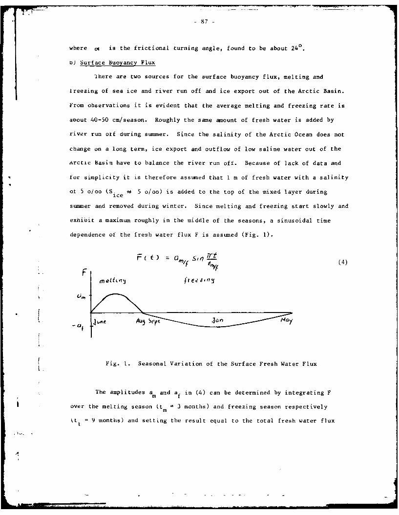
- 87 -

where is the frictional turning angle, found to be about 240.

o) Surface Buoyancy Flux

1here are two sources for the surface buoyancy flux, melting and

freezing of sea ice and river run off and ice export out of the Arctic Basin.

From observations it is evident that the average melting and freezing rate is

aDout 40-50 cm/season. Roughly the same amount of fresh water is added by

river run off during summer. Since the salinity of the Arctic Ocean does not

change on a long term, ice export and outflow of low saline water out of the

Arctic Basin have to balance the river run off. Because of lack of data and

for simplicity it is therefore assumed that 1 m of fresh water with a salinity

ot 5 o/oo (S. 5 o/oo) is added to the top of the mixed layer duringice

summer and removed during winter. Since melting and freezing start slowly and

exhibit a maximum roughly in the middle of the seasons, a sinusoidal time

dependence of the fresh water flux F is assumed (Fig. 1).

F"cf t0S ~ (4)

F IV

t"0

Fig. 1. Seasonal Variation of the Surface Fresh Water Flux

The amplitudes a and af in (4) can be determined by integrating F, mf

over the melting season (t = 3 months) and freezing season respectivelym

U = 9 months) and setting the result equal to the total fresh water flux

* b.

-88-

per season Ul m). The buoyancy flux B associated with this fresh water flux F

is given by

B =-g P F(S-5) (5)

where g is the gravitational acceleration and ( = -£ describes the

dependence of the water density p as a function of the salinity S of the

mixed layer. For T = 00 C and p = po z 0.8 • 10 - 1 [-/00 (Sverdrup, I

johnson, Fleming, 1942).

c) Parameterization of the Dissipation

vot all of the kinetic energy supplied by the keel stirring is used to

entrain water trom below; some part of it is dissipated on its way to the

mixed layer base. Besides the (poorly known) dependence on surface properties

it seems to be appropriate to model the dissipation of kinetic energy due to

mechanical mixing as a function of depth. It also seems reasonable to assume

a cut-off depth H at which all of the kinetic energy input is dissipated.

With the assumption of a linear dependence on depth, the factor m in (2) is

given by

mm I -mH (6)with m I c cos (from Eq. 3). HO

w

During the freezing period, a certain amount of the convective energy

kdescribed by 1-n in Eq. (2)) is dissipated. From laboratory tank experiments [Deardorft, Willis, and Lilly (1969) found that n = 0.015. Farmer (1975)

, J.A

AD-A82 45 WOODS HOLE OCEANOGRAPHIC INSTITUTION MASS F G /81979 SUMMER STUDY PROGRAM IN GEOPHYSICAL FLUID DYNAMICS AT THE ETC(U)NOV 79 M E STERN, F K MELLOR NOOOO-79-C-0671

UNCLASSIFIED WHO0-79G-84VOL-2 NLEaE ////////IEEIIIIEIIIIIIEIIIIEIIIEEEIIIEEIIIEIIIEII-mEEEIIIIIII-mEllllllllllE-IIEIIIIIII.E

-89-

derived a mean of n -0. 036 from observations of a mixed layer under the ice

of a frozen lake. Gill and Turner (1976) obtained the best agreement with

observations of the mixed layer in the North Atlantic when convective stirring

is non-penetrative (n = 0).

From the model described in the following sections, it is found that

the assumption of a cut-off depth H 0in (6) is necessary to obtain a finite

and complete cyclical response of the mixed layer to forcing with cyclical B

(Eq. (5)). The assumption of a cut-off depth is also necessary for n, since

convection and keel stirring would otherwise continuously deepen the mixed

layer from one cycle to the other. Therefore, during the freezing period, n

is taken to be

n =I- H (7)

otherwise n = 1.

d) Model Equations

Eq. (2) and the vertical integral of Eq. (1) rewritten as

We L -' (8)

as W. __ -G-S) (9)At H

represent the two governing differential equations for the polar mixed layer.

The buoyancy step 6 b at the lower interface is proportional to the salinity

step A S, tb = -g fAS ,and no solar radiation penetrates through the

ice, I = 0 in Eq. (2). In Eqs. (8) and (9) S stands for S-S.ic = S-5.

As usual, it is assumed that the mechanical stirring is insufficient to

produce entrainent (w e= 0) during the period of increased melting (in-

* .. creased stability). In this case Eqs. (8) and (9) simplify to

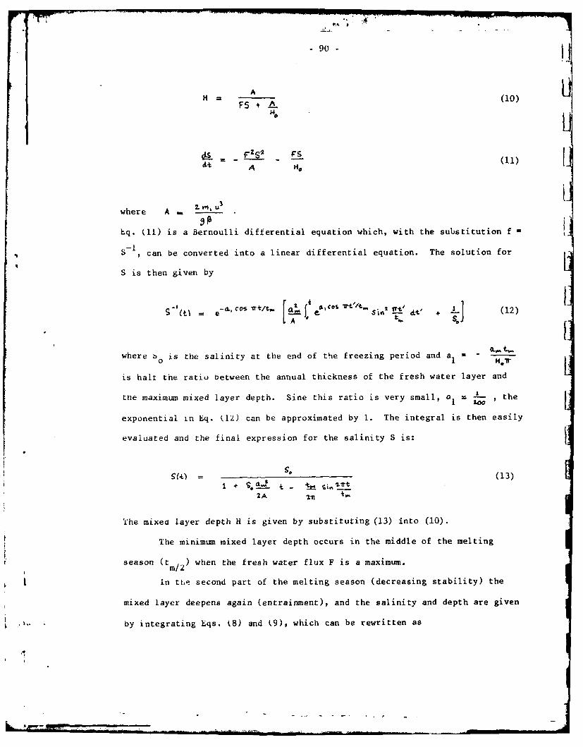
90 -

S= (10)

A HO

where A .

Eq. k1) is a Bernoulli differential equation which, with the substitution f =

S can be converted into a linear differential equation. The solution for

S is then given by

(o, .ne' e'.t ' "' 1 (12)

where b is the salinity at the end of the freezing period and a1 - olt

0

is halt the ratio between the annual thickness of the fresh water layer and

the maximum mixed layer depth. Sine this ratio is very small, 1 -I , the

exponential in Eq. k12) can be approximated by 1. The integral is then easily

evaluated and the final expression for the salinity S is:

9 (-0 0 (13)

2A W

The mixed layer depth H is given by substituting (13) into (10).

The minimum mixed layer depth occurs in the middle of the melting

season (t i/z) when the fresh water flux F is a maximum.

In tte second part of the melting season (decreasing stability) the

mixed layer deepens again (entrainment), and the salinity and depth are given

,b,- by integrating Eqs. (8) and (9), which can be rewritten as

.,o

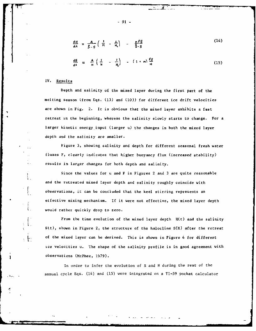
-91-

CL_4_ ,FS14

as A + (15)

IV. Results

Depth and salinity of the mixed layer during the first part of the

melting season (from Eqs. (13) and (10)) for different ice drift velocities

are shown in Fig. 2. It is obvious that the mixed layer exhibits a fast

retreat in the beginning, whereas the salinity slowly starts to change. For a

larger kinetic energy input (larger u) the changes in both the mixed layer

depth and the salinity are smaller.

Figure 3, showing salinity and depth for different seasonal fresh water

fluxes F, clearly indicates that higher buoyancy flux (increased stability)

results in larger changes for both depth and salinity.

Since the values for u and F in Figures 2 and 3 are quite reasonable

and the retreated mixed layer depth and salinity roughly coincide with

V observations, it can be concluded that the keel stirring represents an

etfective mixing mechanism. If it were not effective, the mixed layer depth

would rather quickly drop to zero.

From the time evolution of the mixed layer depth H(t) and the salinity

S(t), shown in Figure 2, the structure of the halocline S(H) after the retreat

V of the mixed layer can be derived. This is shown in Figure 4 for different

ice velocities u. The shape of the salinity profile is in good agreement with

observations (McPhee, 1979).

In order to infer the evolution of S and H during the rest of the

* annual cycle Eqs. (14) and (15) were integrated on a TI-59 pocket calculator

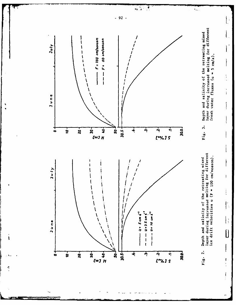
-, 1

-92 A

Cc LOg W

.4 11

I 3,

V, 50) $4

11 4

I U40'- UK

., 0~

C~ >~

S4.-

CDC.cs ..

-93-

0. 0 A-

= %..,-4 0

-4 0 cd

=n *4 "? I

C 4J

all~ 00-

04r2%:~4 .44I

*~~ * *

0 .4 -d

U )

fdC V)I4J 44+4 c C13

a0 $..4 4.. o 4j I

0 W--U> d)

q0 r-q PA

-U 4 4 Im 41 4-4

co r-

0 -4 '-4

24.4 -4

U.4-41co

41' -4

-,4

CS, 0

0>44 4.4 $4 1

C-4 m-

41 W .4

C) 1

~ 0 0

C4 0 ,

"'4.

-94- [

I.0- 3 . S. QA1,1_L.Lt A M!

10 11 H

nu- 2o.

20

30

30.5

Fig. 6. Seasonal variation of the mixed layer depth H and salinity S for fully(dashed-dotted line) and partly penetrative convection (solid line).(Ice drift u = 7.5 cm/s; fresh water flux F 100 cm/season.)

I

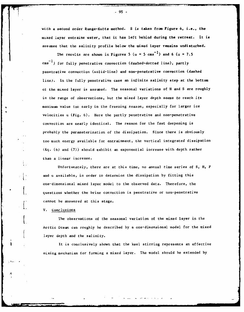
-95-

with a second order Runge-Kutta method. S is taken from Figure 4, i.e., the

Mixed layer entrains water, that it has left behind during the retreat. It is

assumed that the salinity profile below the mixed layer remains undisturbed.

The results are shown in Figures 5 Cu = 5 cas ) and 6 (u - 7.5

cms )for fully penetrative convection (dashed-dotted line), partly

penetrative convection (solid-line) and non-penetrative convection (dashed

line). In the fully penetrative case an infinite salinity step at the bottom

ot the mixed layer is assumed. The seasonal variations of H and S are roughly

in the range of observations, but the mixed layer depth seems to reach its

maximum value too early in the freezing season, especially for larger ice

velocities u (Fig. b). Here the partly penetrative and non-penetrative

convection are nearly identical. The reason for the fast deepening is

probably the parameterization of the dissipation. Since there is obviously

too much energy available for entrainment, the vertical integrated dissipation

(Eq. (6) and (7)) should exhibit an exponential increase with depth rather

than a linear increase.

Unfortunately, there are at this time, no annual time series of S, H, F

and u available, in order to determine the dissipation by fitting this

one-dimensional mixed layer model to the observed data. Therefore, the

questions whether the brine convection is penetrative or non-penetrative

cannot be answered at this stage.

V. Conclusions

The observations of the seasonal variation of the mixed layer in the

Arctic Ocean can roughly be described by a one-dimensional model for the mixed

layer depth and the salinity.

It is conclusively shown that the keel stirring represents an effective

mixing mechanism for forming a mixed layer. The model should be extended by

-96 -

including an equation for the mean horizontal velocity and for the tempera-

ture although the latter one does not seem to be very important. The

parameterization of the dissipation has to be improved, perhaps by fitting [1models to observed data.

Acknowledgements

I would like to thank the GFD Staff, especially K. Hunkins, P.

Killworth and A. Gill, for very stimulating discussions.

REFERENCES

Deardorff, J. W., G. E. Willis and D. K. Lilly, 1969. Laboratoryinvestigation of a nonsteady penetrative convection. J Fluid Mech.,35, 7-31.

Farmer, D. M., 1975. Penetrative convection in the absence of mean shear.Quart. J. R. Met. Soc., 101, 869-891.

Gill, A. E. and J. S. Turner, 1975. A comparison of seasonal thermoclinemodels with observations. Deep-Sea Res., 23, 391-401.

Hunkins, K., L. Bauer and A. Amos, 1977. Salinity and temperaturemeasurements from AIDJEX manned array. Proc. of the Symposium on SeaIce Processes and Models, Sept., 1977, Seattle.

McPhee, M. G., 1975. The effect of ice motion on the mixed layer under Arcticpack ice. AIDJEX Bull., 30, 1-27.

McPhee, M. G., 1978. AIDJEX Oceanographic Data Report, AIDJEX Bull., 39,

33-77.

McPhee, M. G., 1979. Unpublished AIDJEX data, private communication.

McPhee, M. G. and J. D. Smith, 1976. Measurements of the turbulent boundarylayer under pack ice. Jour. Phys. Oceanogr., 6, 696-711.

Niller, P. P. and E. B. Kraus, 1977. One-dimensional models of the upperocean. In E. B. Kraus (ed.) Modelling and Prediction of the UpperLayers of the Ocean. Pergamon Press, 143-172.

SCOR Working Group 58, 1979. The Arctic Ocean Heat Budget. Univ. of Bergen,

Sverdrup, H. U., M. W. Johnson and R. Fleming, 1942. The Oceans,

Prentice-Hall, N. J.

k . ... ..I.. . . . . . . . . .... . . . .. . ... I I II

-97-

STEADY TWO-LAYER SOURCE-SINK FLOW

Lynne Talley

I. Introduction

Ocean circulation can be thought of as being forced almost entirely by

heating and cooling, whether directly, as a result of heat transfer across the

ocean surface, or indirectly by the winds which arise from heating and cooling

of the atmosphere. In this paper we will be mainly interested in extremely

idealized circulation produced directly by cooling and heating. Many simpli-

* fications are made with respect to the flow, the basin geometry and the type

of forcing but it is hoped that insight will be gained into the circulation in

regions where cooling and heating are particularly important. We specifically

have in mind the circulation of the northern North Atlantic, the Norwegian-

Greenland Sea and to a lesser extent, the Labrador Sea. The Norwegian--

Greenland Sea is particularly well known as the source of the cold saline

[ Bottom Water which enters the North Atlantic in deep western boundary currents

and which contributes its characteristics to the North Atlantic Deep Water.

Bottom Water is formed in the large cyclonic gyre occupying the Greenland Sea

from inflowing Atlantic Water (Cartnack and Aagaard, 1973) which enters the

L. Norwegian Sea as the broad northward Norwegian Current. It subsequently

L appears to become more topographically controlled as it strengthens on the

eastern flank of the Jan Mayen Ridge, flows through the gap in the East Jan

F Mayen Ridge and then along the eastern side of the Greenland Basin where it

forms the eastern side of the cyclonic Greenland Sea gyre (Metcalf, 1960).

To some extent, there is a similar process in the Labrador Sea, although

the dense water which is formed there is an Intermediate Water rather than

.ai

-98-

Bottom Water. There also, a cyclonic gyre is the scene of production of dense

water, fueled by the inflow of Atlantic Water in the West Greenland Current

and colder fresher water from the north.

The model discussed here is a steady extension of the time dependent two-

layer model investigated analytically and numerically by Gill (1979b) and the

time dependent axisymmetric model of Gill et. al. (1979). It is a steady two-

layer model, intended for instance to model the upper Atlantic Water and deep

Bottom Water of the Norwegian-Greenland Sea, in which cooling is introduced as

simple mass and momentum transfer from a layer of density p. ,to a layer of

density .We will not concern ourselves with the actual mechanism for

production of denser water, but rather with the resulting circulation. Steady

linear solutions for the baroclinic mode will be sought for various types of

distributed transfer in a meridional channel and then for point transfer in a

horizontally infinite ocean, on the f and pplanes, motivated by the appar-

ent presence of large scale density currents and localized Bottom Water forma-

tion in the Norwegian-Greenland Sea. The effects of bottom friction and

topography are not included.

Formulation in terms of a two-layer model is largely motivated by the

apparent two component nature of the Norwegian-Greenland Sea circulation. We

undoubtedly lose some information about the vertical structure of the flow but

can, nevertheless, see the broad outlines of the forced solution.

We will see that inclusion of diffusion in a steady two-layer model implies

the possibility of eastern boundary layers in both f and L'plane steady

ocean circulation models.

II. Equations

The two-layer system is illustrated in Fig. 1. h I is the variable height

of the upper layer, H2 it etvleadh H1 -h 1= h 2 the height of

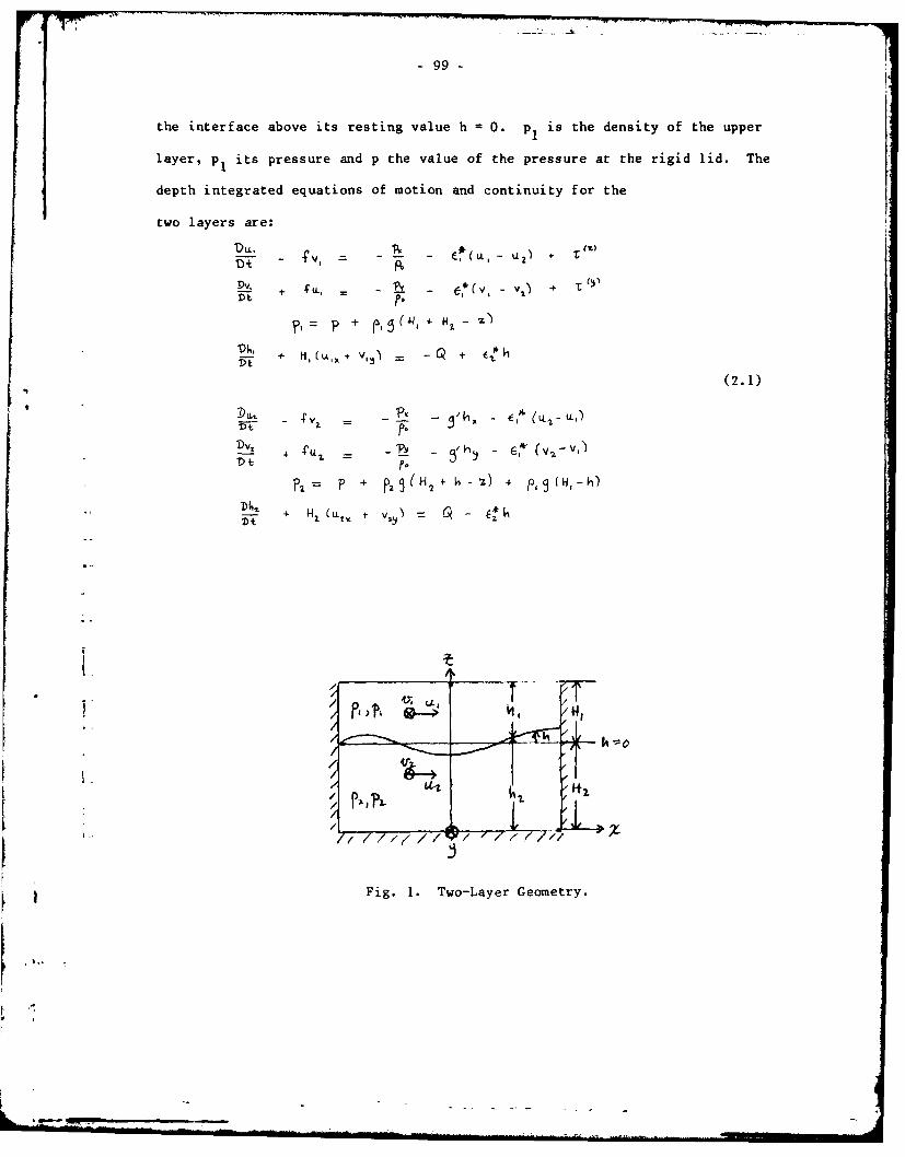
- 99 -

the interface above its resting value h 0 0. pI is the density of the upper

layer, p1 its pressure and p the value of the pressure at the rigid lid. The

depth integrated equations of motion and continuity for the

two layers are:

D-T - 4 , = - -

+)-" = --DU.,

DVI + , + Qh

(2.1)

__ =(v-V

H+ ks) 4 Wo- + =~' P +p? + - ,9(,H

F/14

Fig. 1. Two-Layer Geometry.

- 100 -

I!

II

e

We make the Boussinesq approximation and have already included hydrostatics in

writing the x and y momentum equations where P. LPo Q is the mass

transfer from the top to bottom layer, C' the coefficient of momentum

transfer and g* the coefficient of diffusion. We have also included wind

stress although, in the absence of bottom friction, the barotropic component

of the flow can never be steady. The term E?(h is absolutely crucial for the

existence of steady solutions in the presence of a nonzero mass transfer Q

since continual transfer without damping would imply continual spinup. One

way of obtaining diffusion terms of this form is by using a normal mode analy-

sis. If the buoyancy frequency N is constant, the variations in the vertical

are sinusoidal with a fixed wave number m for each mode. Thus the operator

can be replaced by

+ Km2

for this particular mode, and the latter operator is the one used here. The

coefficient Km2 varies from mode to mode, but here only one is considered.

The same method can be used if N is not constant, but only if the diffusion

coefficient varies with height in a suitable manner.

We look for steady and linear solutions. The appropriate scaling for the

problem is

=Lu == ,____. [~1 = TIL.', L" i, 'j"1. U [ T

where P= P, Itfl, W2

ho

101 -

The resulting nondimensional equations are

-- , - -1 (L - l -L- * ....

v4 . C (2.3)

=.- - £e4h - (:1{Va-V, '+ V, I = , Q - a

where e, =- and ez-

(If the primary driving force were the wind, velocity would be scaled accor-

ding to wind stress T and not mass transfer Qo).o

We would like to look separately at the baroclinic and barotropic flows

and therefore form the sum and difference equations with 5 = u u and

u 2 -u - -2 -l+ + 60[:,'.,

U + -(2 + - .;QoR (2.4a)

and 1 V, H2 (U" +V, 0and

AA

1. * [ o---- -hT. (2.4b)

If we now introduce a stream function V for the baroclinic solution which is

102- L

geostrophic to lowest order h), and arbitrarily assume that 2 1 =

2 , the baroclinic vorticity equation is approximately

-, ( ) (2.5)

The boundary conditions are for no normal flow through any barriers, that

is

L= 0 - at meridional barriers (2.6)

V = t C = at zonal barriers

(In general, the apparently more rigorous conditions u1 = u2 = 0 or vI

v= 0 will be met by solutions with boundary conditions (2.6) as long as no

extra conditions are put on the flow.)

Ill. Meridionally Uniform Flow

i) f plane, c = 0

We will begin with the simplest possible case: steady, meridionally

uniform forcing of the form Q(x) on the f plane with no wind stress, in a

channel of width 2L centered at x = 0. The f plane, y independent vorticity

equation which must be satisfied is

6(h - h) = -Q (3.1a)xx

subject to the boundary conditions LL= - n C C) 91 L

The simplest subcase of this is uniform sinking everywhere, Q A The

equally simple result is that

V A

(3.2)

- 103 -

In other words, the upward motion of the interface due to uniform sinking

everywhere is balanced by upward diffusion everywhere. There are no veloci-

ties associated with this displacement.

If we allow for x variation in the forcing so that Q Ax, the principle

balance in the interior is still between forcing and diffusion (the particular

solution to (2.5) is -'= _ ) • However, because the interface is now tilted,

meridional geostrophic velocities are generated which have zonal O(W) veloci-

ties associated with them. The resulting solution which satisfies the no nor-

mal flow boundary conditions at x = + L is

h = A x - sinhx (3.3)

which is the interior particular solution corrected with boundary layers at

the two walls. In the neighborhood of the wall x = L, the solution (3.3) is

of the form A ( - L) with an exponential boundary layer correction.

The dimensional width of the boundary layers is the Rossby radius R =

If we had retained the separate friction and diffusion parameters 2C, and1!

62 from 2.4b), the dimensional boundary layer width would be -" iAs the "friction" 2G, is increased the boundary layer width increases, and

as "diffusion" c2 is increased, the boundary layer width decreases.2rThe boundary layers result from the deformation of the interface at the

wall caused by the nonzero zonal velocities in the interior. As the interface

is pushed up or down, geostrophic boundary currents are created which in turn

have O(E) zonal velocities associated with them which oppose the interior zonal

.4

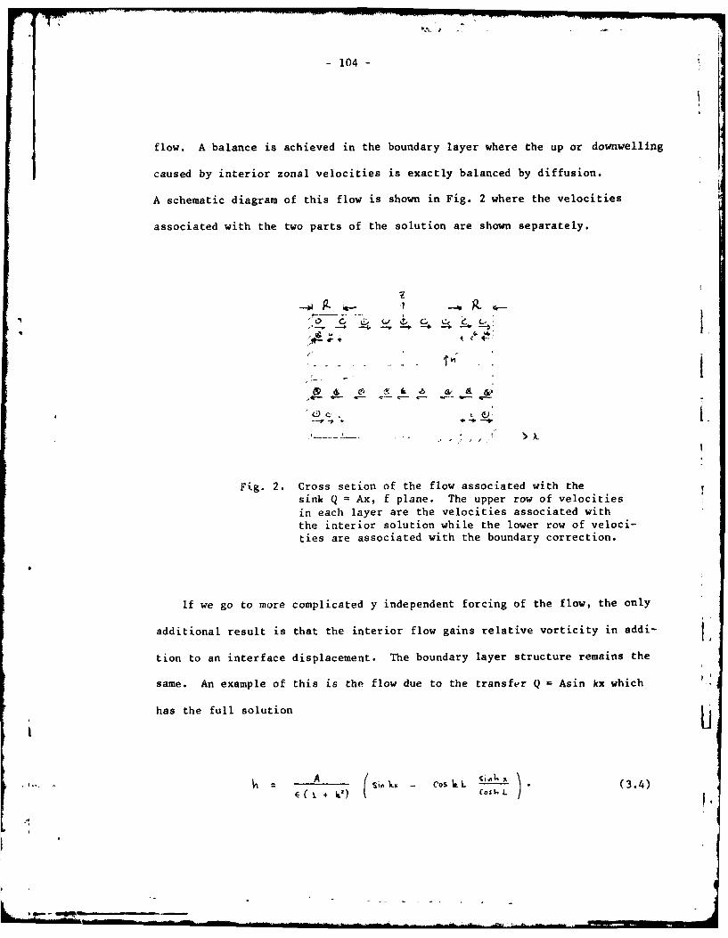
: ; , : .. . .. .. .. .. .. . . . . . . - .. . . . , .- 1

- 104 -

f low. A balance is achieved in the boundary layer where the up or downwelling

caused by interior zonal velocities is exactly balanced by diffusion.

A schematic diagram of this flow is shown in Fig. 2 where the velocities

associated with the two parts of the solution are shown separately.

r{

"' ~~< ... .4-

01

Fig. 2. Cross setion of the flow associated with the

sinh = Ax, f plane. The upper row of velocities

in each layer are the velocities associated with

the interior solution while the lower row of veloci-

ties are associated with the boundary correction.

If we go to more complicated y independent forcing of the flow, the only

additional result is that the interior flow gains relative vorticity in addi-

Lion to an interface displacement. The boundary layer structure remains the

same. An example of this s the flow due to the transfer iAsin kx which

has the full solution iut-

.... =A ( Si nk 6 os k It L. (3 .4 )tIes ae ad w the b

A -. Cs.. . .(3.4

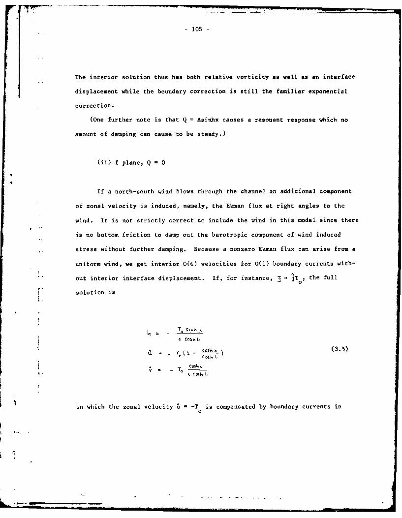
- 105 -

The interior solution thus has both relative vorticity as well as an interface

displacement while the boundary correction is still the familiar exponential

correction.

(One further note is that Q = Asinhx causes a resonant response which no

amount of damping can cause to be steady.)

(ii) f plane, Q = 0

If a north-south wind blows through the channel an additional component

of zonal velocity is induced, namely, the Ekman flux at right angles to the

wind. It is not strictly correct to include the wind in this model since there

is no bottom friction to damp out the barotropic component of wind induced

stress without further damping. Because a nonzero Ekman flux can arise from a

uniform wind, we get interior O(e) velocities for 0(0) boundary currents with-A

out interior interface displacement. If, for instance, t jT , the full

solution is

T. Sivk

e CotL.

A -- - - )_,Coik L

i / _To CostX

c- cav L

in which the zonal velocity O = -T is compensated by boundary currents in0

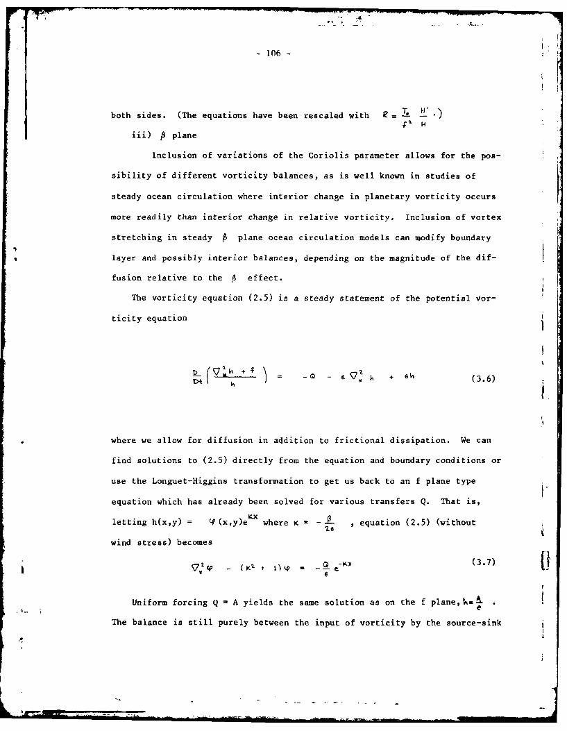
-106-

both sides. (The equations have been rescaled with e= T ')

iii) A plane

Inclusion of variations of the Coriolis parameter allows for the pos-

sibility of different vorticity balances, as is well known in studies of

steady ocean circulation where interior change in planetary vorticity occurs

more readily than interior change in relative vorticity. Inclusion of vortex

stretching in steady A plane ocean circulation models can modify boundary

layer and possibly interior balances, depending on the magnitude of the dif-

fusion relative to the A effect.

The vorticity equation (2.5) is a steady statement of the potential vor-

ticity equation

D . (3.6)

where we allow for diffusion in addition to frictional dissipation. We can

find solutions to (2.5) directly from the equation and boundary conditions or

use the Longuet-Higgins transformation to get us back to an f plane type

equation which has already been solved for various transfers Q. That is,

letting h(x,y) = (?(x,y)e x where K --- , equation (2.5) (without

wind stress) becomes

9 V - (K'- + 1 ) -(x (3.7)

Uniform forcing Q A yields the same solution as on the f planefi= .e

The balance is still purely between the input of vorticity by the source-sink

.4i

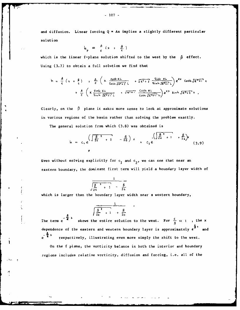
- 107 -

and diffusion. Linear forcing Q = Ax implies a slightly different particular

solution

=A (X+

which is the linear f-plane solution shifted to the west by the A effect.

Using (3.7) to obtain a full solution we find that

A ) +Co,*1 K I-'4 I_ k'C_ Cos k J W Tj L s i n J 1c +7 ,/

A ( ii 1 Cosiq KL

Si.il' FK4 L CoSh . "

q Clearly, on the ( plane it makes more sense to look at approximate solutions

in various regions of the basin rather than solving the problem exactly.

The general solution from which (3.8) was obtained is

a( J- 2 1 ) ( -1 'c C2 e (3.9)

Even without solving explicitly for cI and c2 9 we can see that near an

eastern boundary, the dominant first term will yield a boundary layer width of

+

J 2C 2

which is larger than the boundary layer width near a western boundary,

2&

The term e skews the entire solution to the west. For - i , the x

dependence of the eastern and western boundary layer is approximately e * and

e-6 respectively, illustrating even more simply the shift to the west.

On the f plane, the vorticity balance in both the interior and boundary

regions includes relative vorticity, diffusion and forcing, i.e. all of the

/4

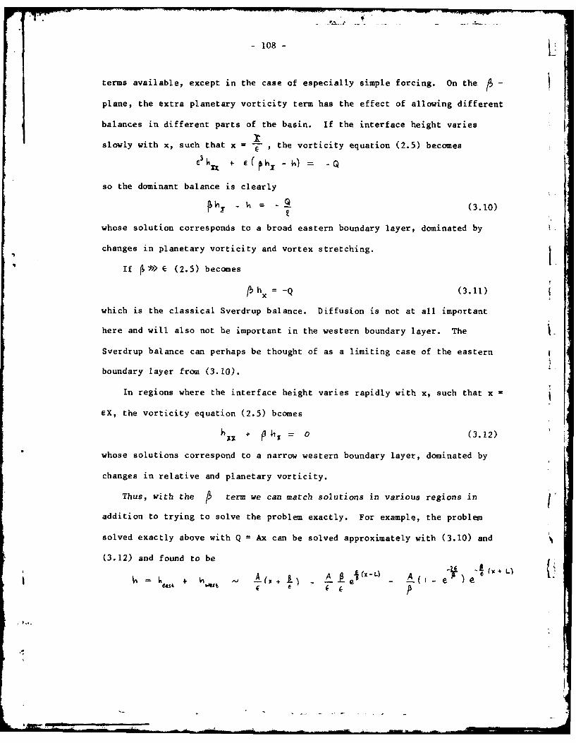
-108 L

terms available, except in the case of especially simple forcing. On the -

plane, the extra planetary vorticity term has the effect of allowing different

balances in different parts of the basin. If the interface height varies

slowly with x, such that x = , the vorticity equation (2.5) becomes

f3 k E(h x -) = -Q

so the dominant balance is clearly

- = - (3.10)

whose solution corresponds to a broad eastern boundary layer, dominated by

changes in planetary vorticity and vortex stretching.

If e 3 (2.5) becomes

hx = -Q (3.11)

which is the classical Sverdrup balance. Diffusion is not at all important

here and will also not be important in the western boundary layer. The

Sverdrup balance can perhaps be thought of as a limiting case of the eastern

boundary layer from (3.10).

In regions where the interface height varies rapidly with x, such that x =

EX, the vorticity equation (2.5) bcomes

0 (3.12)

whose solutions correspond to a narrow western boundary layer, dominated by

changes in relative and planetary vorticity.

Thus, with the term we can match solutions in various regions in

addition to trying to solve the problem exactly. For example, the problem

solved exactly above with Q f Ax can be solved approximately with (3.10) and

(3.12) and found to be

(X -- -Lx+)+- V A l *(K-L A , e ) eWAi e C-

109 -

a substantial simplification of (3.8) for

On both the f and P planes we see that eastern and western boundarylayers occur whenever the interior zonal velocity is nonzero, whether it is

forced directly as an Ekman flux by the wind or more indirectly as a result of

the geostropic flow due to divergences created by mass transfer or wind stress

curl. Steady solutions with this boundary layer structure are possible only

because of the diffusion term eh which allows a damped form of vortex stretch-

ing to occur in steady flow.

With the structure of solutions on the f and planes for meridionally

uniform flow in mind, we move to forcing which may vary with latitude.

IV. Zonally Uniform Forcing in a Meridional Channel

What is the result of cooling which varies with latitude? As a simple

case, we will consider cooling which is uniform and positive (transfer to the

lower layer) in a northern basin and zero to the south with a transition region

I

between which is wider than the Rossby radius but not as wide as . (We

could equally well choose any uniform value for the two halves of the basin.)

We have in mind an enclosed sea like the Norwegian Sea bu: make the simplifica-

tions that a) the basin length is greater than - and b) curvature of the

* basin occurs on a scale larger than the Rossby radius.

The geometry we are considering is illustrated in Fig. 3. For simplicity

we will assume that Q - A for y > 0, Q = 0 for y < -M and Q = A(l + y) in

the transition region. This will necessarily lead to discontinuity in the

zonal velocity at y = 0, -M but is simple to solve, and has the essential fea-

tures or a solution with smoother forcing.

The vorticity equation becomes

r - = - (4.1a)

110- V

subject to the boundary conditions

u = -hy - eh = 0 at x +Lx-

h = 0 at y =-M (4.1b)

h continuous at y = 0

We consider the solution in three stages: i) solution for -M < y < 0 with no x

dependence, ii) solution near x ± L with large scale variation in y and iii)

matching the solutions in the corner near x = L, y = 0. It will be seen that

variation in forcing Q with latitude allows Kelvin wave-like disturbances to

be found far to the north in the region of uniform Q which would otherwise be 1.undisturbed. Thus we may in some way be able to model a more global forcing .

of the eastern boundary current in the Norwegian Sea than we could otherwise

obtain with local winds and forcing.

i) The solution for -M < y 4 0 with = 0 is just the particular solu-

tion

M (4.2)

which has a zonal geostrophic velocity u = - A and meridional Ekman velocity

v- A associated with it. Thus for A > 0, there is an eastward (and

V M

northward) density current in the upper layer and the opposite in the lower

layer.

ii) In the regions where Q = A and Q =0, we stretch the y coordinate by c

so that y 1 . The vorticity equation (4.1a) is then approximately (to 0(e)

Sxx - h

subject to the boundary conditions

A

u ~h+ x) 0 t7

-111 -

Letting

Cj~ L -(x+ L)h = A + Cl(Y)e x - + C2( e-XL

2m

the only solution which decays away to the north, where Q = A, is

h = A + C e Y+x-L

and likewise, the solution which decays away to the south, where Q = Oisy- ( i-L)

h=c e

if there were a wall to the south at x = -L. These correspond to boundary

layers with width equal to the Rossby radius Ro and length of -- , decay-

ing away from the region of varying Q. Considering only the solution to the9

north, the constant cI can be determined by matching transports in the boun-

dary layer at y = 0 with the eastward transport in -M < y < o. We thus obtain

_ -, L )(4.3)A (1 - e A>0

for the boundary layer decaying away to the north.

iii) In the corner near y - 0, x = L, the vorticity equation is

subject to the boundary condition

u = -h = 0 at x = L

h = 0 at y = -M

h = A(l-e x - L ) at y = 0

The vorticity equation is separable and the solution which fits the boundary

conditions is

1- -M I J < 0 (4.4)

.. ......I

112 -

The full solution for the basin is

'A (i- -

+- ) -M<j <6 (4.5)

We note particularly that the zonal velocity is identically zero for y > 0

(a characteristic of a Kelvin wave) and that there is a nonzero geostrophic

meridional velocity along the eastern coast for y > 0 which is solely due to

the variation in Q from - M < y 0 0. The upper layer velocities associated

with the interface displacement (4.5) are shown schematically in Fig. 3.

9X L

- I 3" // / /I., /

Fi.3. Geometry and velocities when Q = Q(y): specifically,Q = A for y > 0, Q = A(I + y) for -M 4 y ' 0 and Q = 0for y< -M. M

It appears then that the steady signature of the Kelvin wave, which would

arise in the time dependent case and travel up the eastern coast to the north,

~is a boundary current which eventually damps out to the north due to fric-

tion. Therefore, even in a region where variation in forcing is too weak to

'"" provoke a flow, there can be flow due to variation in the forcing elsewhere

113 -

(if variation is on a scale less than 1). The mechanism is quite simple: the

eastward flowing density current (upper layer) reaches the wall and causes a

downward displacement of the interface which eventually reaches a diffusive

equilibrium. Geostrophic velocities to the north (upper layer) along the

boundary result and damp out on the frictional scale 1. (The Ekman velocity

associated with the geostrophic velocity in the region -M 4 y < 0 balances the

incoming flow so that it is zero at the wall). Zonal Ekman velocities in the

northward extension which are generated by the geostrophic northward veloci-

ties are exactly balanced by geostrophic zonal velocities due to the variation

in interface height with latitude y (as a result of damping).

Extension of these results to the 0 plane is quite simple and involves

expanding the eastern boundary layer width by 6 (for e « I), the familiar

skewing of the circulation to the west. Damping to the north also occurs over

a scale expanded by G. If we think of the boundary current as a damped Kelvin

wave, the extension of the layer to the west can perhaps be thought of as

damped nondispersive Rossby waves.

Combination of variation of forcing with both latitude and longitude can

thus give rise to wide eastern boundary currents and narrow western boundary

currents. Forcing in the Norwegian-Greenland Sea is irregular but the general

trend is for much higher heat flux to the north (Bunker and Worthington, 1976)

and a general cyclonic wind stress pattern. The wide northward flowing eastern

boundary current which is observed in the southern Norwegian Sea (Metcalf,

1960) may be the result of latitudinal variation in cooling and/or wind stress

south of the entrance to the Norwegian Sea, local northward or cyclonic wind

stress, or local cooling. We note that an eastern boundary current at a

particular latitude can be caused only by 1) local forcing which

L,

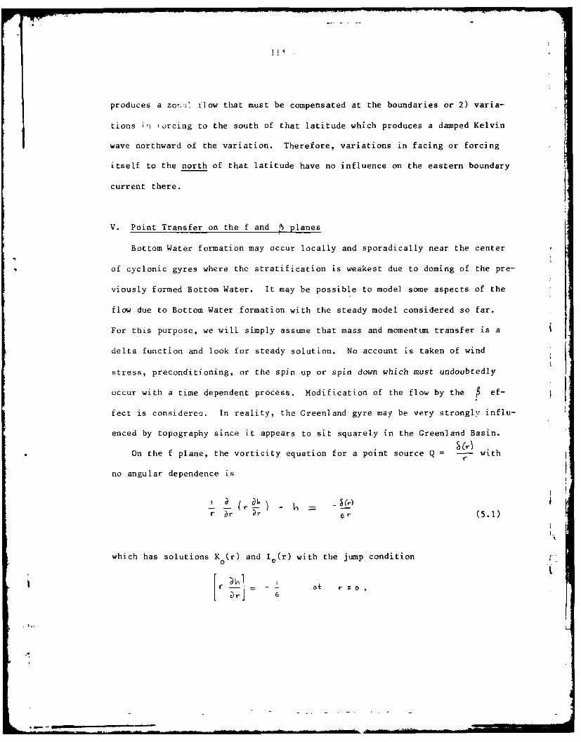
produces a zonal tilow that must be compensated at the boundaries or 2) varia-

tions iH jurcing to the south of that latitude which produces a damped Kelvin

wave northward of the variation. Therefore, variations in facing or forcing

itself to the north of that latitude have no influence on the eastern boundary

current there.

V. Point Transfer on the f and . planes

Bottom Water formation may occur locally and sporadically near the center

of cyclonic gyres where the stratification is weakest due to doming of the pre-

viously formed Bottom Water. It may be possible to model some aspects of the

flow due to Bottom Water formation with the steady model considered so far.

For this purpose, we will simply assume that mass and momentum transfer is a

delta function and look for steady solution. No account is taken of wind

stress, preconditioning, or the spin up or spin down which must undoubtedly

occur with a time dependent process. Modification of the flow by the ef-

fect is considerea. In reality, the Greenland gyre may be very strongly influ-

enced by topography since it appears to sit squarely in the Greenland Basin.

On the f plane, the vorticity equation for a point source Q with

no angular dependence is

r ar Dr er (5.1)

which has solutions K (r) and I,(r) with the jump condition0

-I at r z owir-

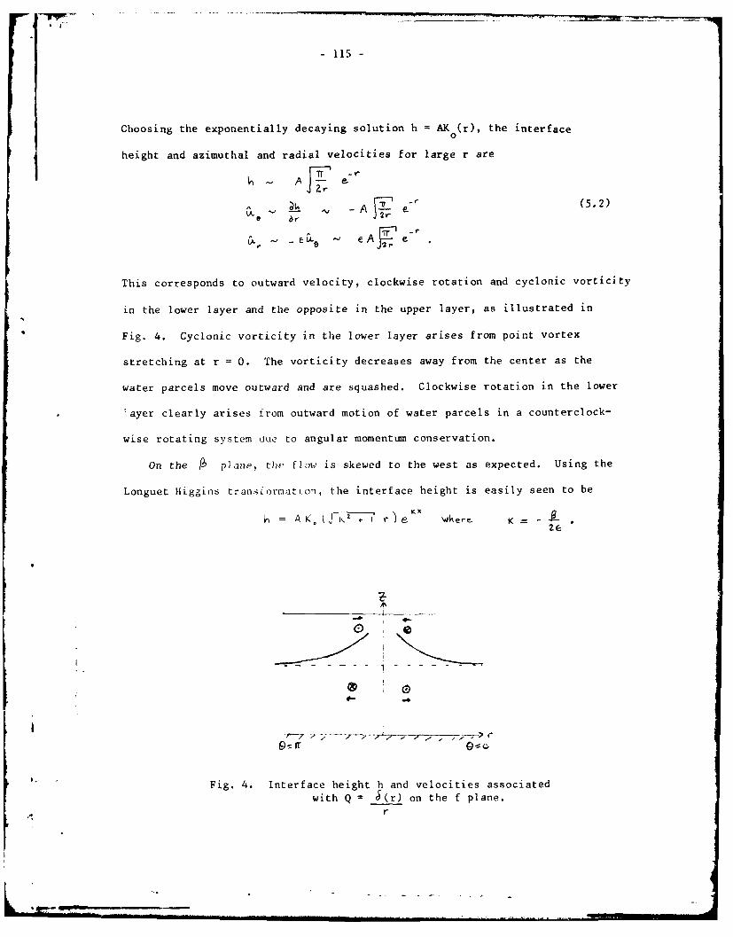
- 115 -

Choosing the exponentially decaying solution h = AK (r), the interface0

height and azimuthal and radial velocities for large r are

ir -r

A T (5.2)

S ~rCA -.- v - A e

This corresponds to outward velocity, clockwise rotation and cyclonic vorticity

in the lower layer and the opposite in the upper layer, as illustrated in

Fig. 4. Cyclonic vorticity in the lower layer arises from point vortex

stretching at r = 0. The vorticity decreases away from the center as the

water parcels move outward and are squashed. Clockwise rotation in the lower

7ayer clearly arises from outward motion of water parcels in a counterclock-

wise rotating system due to angular momentum conservation.

On the P plane, the flow is skewed to the west as expected. Using the

Longuet Higgins transformatLon, tile interface height is easily seen to be

A 4KO~t~ re K" we~i K -26

4-

, i~y -,-.

Fig. 4. Interface height h and velocities associated

with Q S(r) on the f plane.

r

- 116 -

For large r, this becomes / .r(-J7r7T 4 Kccos e)A ?eA r

11 = - is sufficiently large, we have

0 --( - C's 9)

h A ir e~ (-ogOr

The loci of constant phase r(l-cos e) are parabolas which open to the west

(Rhines, 1979 lecture notes) and mass transfer is clearly predominantly to the

west.

Thus, on both the f and f planes, a point transfer of mass and momentum

generates a steady counterclockwise flow in the upper layer and clockwise flow

in the lower layer with the highest velocities near the transfer point. This

type of flow in the upper layer accords with observations of counterclockwise

flow in the Greenland Sea (Metcalf, 1960). It is, however, not to be forgotten

that the wind stress in this region also yields a counterclockwise gyrelso per-

haps the effects reinforce each other in the production of the gyre and in

Bottom Water formation.

VI. Summary

Inclusion of a representation of diffusion in the continuity equation

appears to be a useful way of damping the circulation resulting from a steady

transfer of mass and momentum from one layer to another. With this term in-'s

cluded in the vorticity equation it is possible to meet boundary conditions on

the flow with boundary layers since the interface displacement at the bound-

aries can be an equilibrium between upwelling and diffusion.

The usual steady circulation models on the f plane cannot have eastern

-117

boundary layers because there is no way to balance relative vorticity acces-

sion and changes in planetary vorticity on the eastern boundary. It is for

this reason that boundary layers occur only in the west while the balance else-

where is between forcing and changes in planetary vorticity (Sverdrup balance),

in the usual ( plane models. Inclusion of damping of vortex stretching in

the form of the diffusion term ch in the vorticity equation allows the presence

of western and eastern boundary layer's. The western boundary layer still has

the same structure as before, but the interior (eastern) solution includes dif-

fusion as well, as long as is not too small.

Application of these results to the actual flow in the Norwegian-Greenland

Sea may be somewhat tenuous but two features deserve mention. The first is the

broad northward Norwegian Current which may possibly be modelled as the north-

ern damped Kelvin wave extension of an eastward density or wind driven current

in the northern North Atlantic. The second is the counterclockwise circulation

in the Greenland Basin which may be partially driven by the formation of Bot-

tom Water at its center and may be roughly modelled by the point transfer of

Topography and wind may play a very large role in determining the actual

Acknowledgements

I would like to express my gratitude to Dr. Adrian Gill for his patience

*in outlining the problem and help in understanding some of the rudiments of

ocean modelling. The advice that he and other members of the Staff gave for

* formulating, carrying out, and talking about a research problem is much

appreciated.

REFERENCES

Bunker, A. F. and L. V. Worthington, 1976. Energy exchange charts of theNorth Atlantic Ocean. Bull. Am. Meteor. Soc., 57, 670-678.

Carmack, E. and K. Aagard, 1973. On the deep water of the Greenland SeaDSR, 20, 687-715.

Gill, A. F., J. M. Smith, R. P. Cleaver, R. Hide and P. R. Jonas, 1979. Thevortex created by mass transfer between layers of a rotating fluid.

Geophy. and Astrophy. Fluid Dynamics, 12, 195-220.

Gill, A., 1979. GFD Lectures.

Rhines, P., 1979. Class notes from "Mesoscale Ocean Dynamics".

Uii

iB

- 119 -

A Study of Thermal Convection in a Rotating Annulus

with Applied Wind Stress and Surface Velocity

David Topham

I. Introduction

The circulation arising from a non-uniform distribution of surface

temperature was suggested by Stommel as a model of oceanic circulation. It

was proposed that heating at the equator would produce a thermocline in which

downward thermal diffusion was balanced by upward convection flows. The

sinking convective flows were confined to a small region at the poles

(Stommel, 1958).

The broad features of this model were confirmed by laboratory experiments

for a nonrotating system by Rossby (1965) who applied a linear temperature

gradient to the bottom of a box, insulated on its other surfaces. The heat

exchange was confined to a thin boundary layer at the bottom, while the con-

vectively driven flow rose in a narrow plume against the hot wall. The in-

terior fluid was almost uniform with a temperature excess approaching 70% of

the maximum imposed temperature difference.

The corresponding problem in a rotating annulus has been solved by Stern

(1975) for strong rotation with a linear temperature distribution. While

Killworth (1979) considers the general problem and derives scaling parameters

which identify six distinct flow regimes, ranging from the nonrotation case of

Rossby to a limiting case of very strong rotation for which the convection

flows are suppressed and a purely diffusive heat balance obtains. Killworth

presents numerical computations of a special similarity solution ranging from

no rotation to medium rotation conditions. The general effect of rotation is

to inhibit the radial velocities and confine them to narrow Ekman layers.

-120-

This restriction of the convective flows causes a thickening of the thermal

layer and a reduction of heat transfer in the system. In the strong rotation

case considered by Stern the interior region of the fluid outside the thermal

boundary layer assumes the temperature of the hottest end of the heated

boundary. The rotating annulus has been explored in the laboratory by Hignett

(1979) up to the medium rotation range. A wave-like instability was found for

the higher rotation rates.

The problem addressed here is a modification of the rotating annulus in

which additional boundary conditions are imposed, over and above that of the

surface temperature distribution. In particular, two modifications of the

conditions at the heated boundary are considered, an imposed distribution of

surface velocity and an imposed distribution of surface stress. These

additional boundary conditions can be arranged to either enhance or oppose the

thermally driven flows; both cases are discussed. Both temperature and

mechanical boundary conditions are considered to be applied at the bottom of

the annulus.

2. Analysis

The following hierarchy of problems has been considered:

i) The rotating annulus with an applied variation of surface velocity and

very small temperature difference, such that the heat can be regarded as a

passive contaminant.

ii) The strong rotation case with strong thermal effects and small changesL

in the bottom velocity distribution, ie., weak mechanical driving.

iii) The limiting case of (ii) with strong mechanical driving

a) to enhance the thermal flows

b) to oppose the thermal flows.

121

iv) The strong rotation case with strong thermal effects where the

boundary condition imposed is one of stress rather than velocity.

The notation employed follows that of Killworth (1979). The annulus is

taken to have a radial separation L and height H, curvature is neglected and

the origin is taken at the bottom lefthand corner, with the x-axis horizontal

and the z-azis vertical. The imposed temperature along the x-axis (bottom)

has its cold end at the origin. There is no variation of any of the

parameters in the y direction. The buoyancy is defined as

a' =

where , is the density at the origin, g is the acceleration due to gravity,

and primes denote dimensional variables.

The following seven dimensional quantities determine the system:

m the maximum imposed buoyancy difference

L,H, the dimensions of the annulus

V, the kinematic viscosity

K, the thermal diffusivity

f, the Coriolis parameter

v' the maximum velocity imposed at the bottom boundary or in thes

case of stress driven systems aYi is imposed.

From these the following nondimensional parameters can be formed:

- R_ . , the Rayleigh number (2.1)

_ E the Ekman number (2.2)1..

o _~j r" a : .zv"- . n . .. . . . ... . .. . . I

122 -

- = , Prandtl number (2.3)K

'I

H , the aspect ratio (2.4)L

= ,Peclet number, velocity (2.5)K

boundary condition

L ( Peclet number, stress (2.6)

K

boundary condition

In addition, the form of the applied distribution of v and AV)SS -o

will influence the problem.

The following additional parameters are defined to facilitate comparison

with the thermal driven results. Killworth demonstrates that the ratio of the

thicknesses of the thermal and Ekman layers is the fundamental parameter

determining the character of the thermally driven flows and defines

R .l s " LIS 2/6

c L 2 or Qa K- (2.7)

Q therefore is a measure of the rotation rate of the system. Rossby showed

that the thermal thickness scaled as Ra- /5 and the Ekman layer scales as

• E1 / 2

E11 ., Q is the square of the ratio of these thicknesses.

-

- 123-

It is also convenient to introduce the parameter F in the case where a

velocity boundary condition is imposed, where

F= = a-' EP,Lf (2.8)

In the laboratory the use of water as a working medium gives the following

orders of magnitude of the above parameters:

R - 10a

E 10- 4

r 10

~ 1

P 2 x 102

v

F 1 0- 1 to I

The equations of motion can be written in the form

Vorticity

v ' , = '- v' - -' 7 '~(2.9)

Zonal momentum

V V, + zi(" )v 7tv' :" ' + (v',V')(2.10)

Buoyancy

+ / 0 (2.11)

,4

A

124 -

The absence of variation in the y direction implies the stream function

such that

-L (2.12)

VLis the Laplacian operator and J the Jacobian operator

J(a,b) = axbz - a2bX, where the coordinate z takes on its appropriate

scaled form for the different regimes considered.

For the case where the surface velocity v is prescribed the boundarys

conditions are

V' -X) 0 0 V

V- , = v= A, = 0 Ca -H (2.13)

0 = ' & '= 0,

An additional constraint is that there be no net heat flux from the fluid,

expressed as

* fL

0Al 0 on a'= o (2.14)

Killworth (1979) and Killworth and Manins (1979) consider that the solu-

tion of the horizontal boundary layers and the interior is fully determined

without a detailed consideration of the structure of the sidewall boundary

layers. The sane will be assumed for the modified bottom boundary conditions

considered here.

b...

... .-.4 . . ] :" I III |

:i i. ... ' " . . . -- -

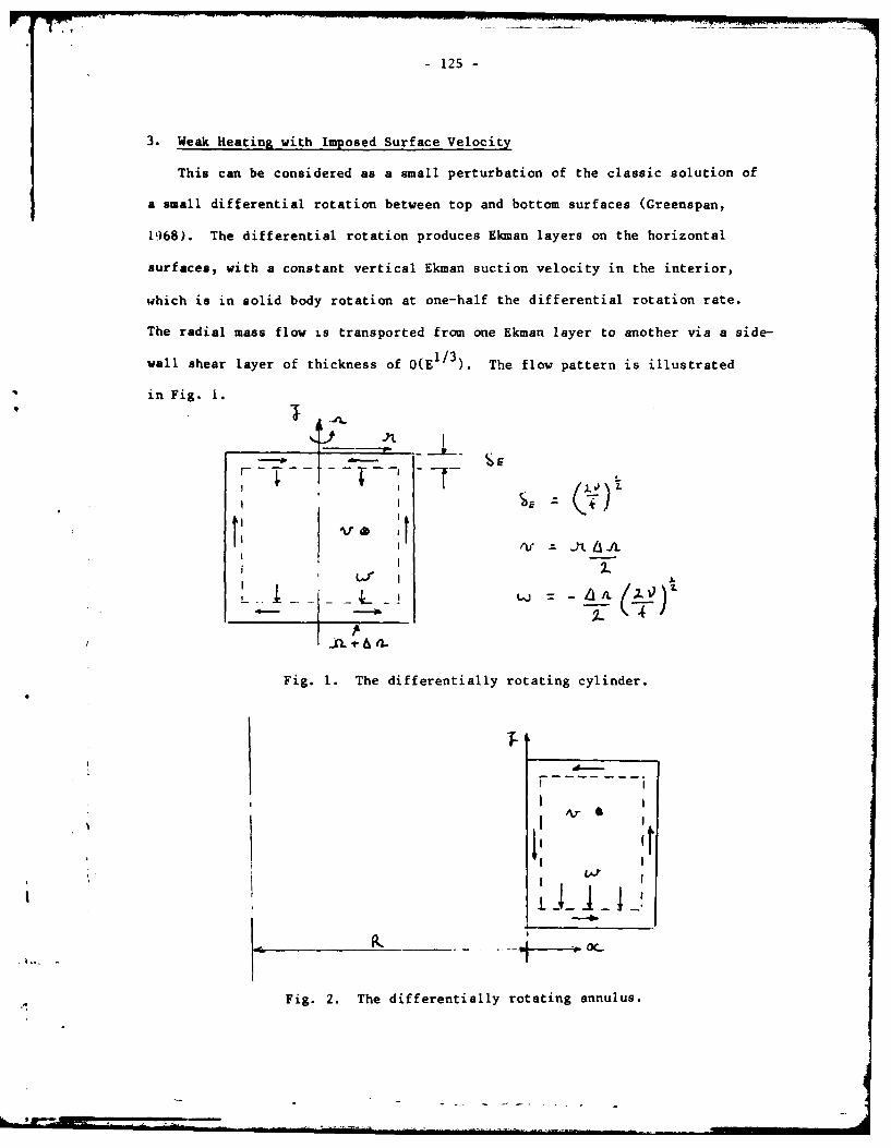
- 125 -

3. Weak Heating with Imposed Surface Velocity

This can be considered as a small perturbation of the classic solution of

a small differential rotation between top and bottom surfaces (Greenspan,

1968). The differential rotation produces Ekman layers on the horizontal

surfaces, with a constant vertical Ekman suction velocity in the interior,

which is in solid body rotation at one-half the differential rotation rate.

The radial mass flow is transported from one Ekman layer to another via a side-

wall shear layer of thickness of O(E1 /3). The flow pattern is illustrated

in Fig. 1.

r -

tiV 'V@

L .I 1-

..... . _. & = -

Fig. 1. The differentially rotating cylinder.

I A

I V i

_ __ _ _OC

Fig. 2. The differentially rotating annulus.

P.-126-

If the annulus is considered as a geometrical extension of the differen-

tially rotating cylinder, the velocity distribution on the bottom is given as

v = 6r C R + x); the mass flow in the Ekman layers and t-he interior flow

v increase as CR + x) and the vertical velocity w is unchanged. The interior

wall now requires a second vertical shear layer to balance the flow in the

Ekman layers (Fig. 2). In the work which follows the geometrical constraint

on the form of the imposed surface velocity, namely vs = nn (R+x)

is relaxed and more general velocity distributions considered.

in practice it is found that the linear distribution vs = o , x' affords

the greatest mathematical simplification while retaining the essential physi-

cal features of the problem. In particular, it provides a vertical velocity

* which is independent of x, which affords considerable simplification in the

strongly heated cases. The effects of weak heat addition to such a velocity

driven system are now considered; the lower limit in which the heat acts as a

passive contaminant is defined as the point where the velocity field is

unaffected by the temperature field. Consider now the scaling appropriate to

such a limit, where the imposed surface velocity is given by the relationship

The vertical velocity associsted with this is

Making use of the definition of Ekman number (2.2) and the parameter F (2.8),

yields the appropriate scaling for the stream function.

127 -

The accompanying scaling for v' and A: are

v' = YFL-1 v and A' A A , with a thermal layer.

8TH= L F_1 El12, where appropriate.

Take equations of motion in the interior, where both x'and z'are scaled

with L, take the form

Vorticity

ES/I = IEF 'I' A - v F FJ(V, IQ 2V) (3.1)

Zonal Momentum

(3.2)E'/I 7Tv = + FE.T(v,1 ')

Buoy ancy

.Vz .+ FE'/" 2,(,A) = o (3.3)

For the interior flows to be undisturbed it requires that

E << 1, F < E - and Ra << FE 1

if the low Rossby number velocity field is to be retained.

For the typical laboratory values quoted for water in the introduction the

first two conditions are satisfied and the third requires that Ra << 103

say 10 2 , which would correspond to a maximum temperature difference of

10-5 oC across a 10 cm annulus, a weak heating indeed! There are two

possibilities for the balance of the thermal layer; firstly, that the imposed

vertical velocity is away from the heated wall, in which case no convective-

* 1.. , ] i ,

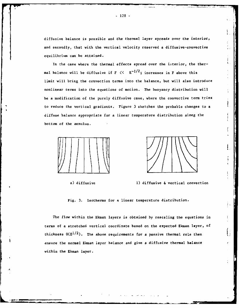
-128-

diffusive balance is possible and the thermal layer spreads over the interior,

and secondly, that with the vertical velocity reserved a diffusive-convective

equilibrium can be attained.

In the case where the thermal effects spread over the interior, the ther-

mal balance will be diffusive if F << E-1/ 2 ; in creases in F above this

limit will bring the convection terms into the balance, but will also introduce

nonlinear terms into the equations of motion. The buoyancy distribution will

be a modification of the purely diffusive case, where the convective term tries

to reduce the vertical gradients. Figure 3 sketches the probable changes to a

diffuse balance appropriate for a linear temperature distribution along the

bottom of the annulus.

a) diffusive 1) diffusive & vertical convection

Fig. 3. Isotherms for a linear temperature distribution.

The flow within the Ekman layers is obtained by rescaling the equations in

terms of a stretched vertical coordinate based on the expected Ekman layer, of

thickness 0(El/2). The above requirements for a passive thermal role then

ensure the normal Ekman layer balance and give a diffusive thermal balance

within the Ekman layer.

- 129 -

The second possibility, now arising from an Ekman section velocity towards

the heated boundary, requires a further scaling of the equations to account

for the smaller thermal layer thickness, now assumed to be small, compared to

the height and of order K/w.

Thus ,,/L - K/LW - K/L Y FIE/ 2

and the rescaled equations become

Vorticity

F3 V 4 -Y = RaF-2E 5 / 2 n - v. - F 3 J( '7 N ) (3.4)

Zonal Momentum

F V7 Iv = Z + FJ(v, V (3.5)

Buoyancy

2 + 0 (3.6)

For a distinct thermal layer to exist, with an interior region above it,

we require that 6r./L < I and also if the Ekman layer is to be thin, that

<< i. The condition that k./L = F -E/ < 1 can only be

obtained for large values of F, which in turn implies that the nonlinear terms

play a part in the equations of motion. Thus it is not possible to retain the

low Rossby number flows of the mechanically driven system and have a distinct

thermal layer with heat acting as a passive contaminant. For low Rossby

number flows it is only possible to have a distinct thermal layer when the

thermal effects play an active part in the dynamic balance. The coupled

system is considered in detail in the next section.

130 -

4. Strong Rotation and Heating with Weak Mechanical Driving

This is an extension of the case treated by Stern (1975) and by Killworth

for which an explicit solution can be obtained. The qualifications of strong

heating and strong rotation ensure that the Ekman layer is thin compared to

the thermal layer, which in return is thin compared to the height of the

annulus.

Killworth's scaling for this case is

V' K Q1x

,, 1< 1 oY Q" L' V,

with the buoyancy layer of thickness H = L Ra -I 5 Q

The interior equations become

Vorticity

x = /Q / A,- Ro. o"V 5(n,V'K) (4.1)LI/S ~ 3 3/2-/'

Zonal Momentum4

+ - - ( 4 .2 )

Buoyancy

+ + /e-'(,, A' - 0 (4.3)

The requirement that there is to be no thermal wind in the interior is that

Ra4 / 15 >> Q i

* 1.i

-131 -

which yields a homogeneous interior with X z .

Within the thermal layer a new stretched coordinate is defined,

I"= ZL-IRal/5Q-3/4

and the rescaled equations become

Vorticity

Q-/ 4 X = - (4.4)

Zonal Momentum

-S. x /6z "'/Q-5(, - .) (4.5)

Buoyancy

+ o (4.6)

or since the thermal layer is thin

6j -4 -T ( x = o

A further scaling appropriate to the Ekman layer of thickness E = LE '2

defines the stretched coordinate as e = vI L"' R.Ys Q '1%

yielding

X = 0( $/ (4.7)

* =sl") (4.8)

Aee = <(Y.A - )< , << (4.9)

Ge

-132-

t.Thus the Ekman layers are unchanged by the buoyancy to leading order.

Consider now that an arbitrary distribution of velocity is specified on

the heated boundary

Av = O (x)S

The Ekman layer solutions become

r 1x

Cos ( ~ (4.11)

VY.

L= ,= J1 , e' (4.12)

S(4.13)

where the subscript zero denotes conditions just outside the Ekman layer.

In the thermal layer, the buoyancy equation (4.6) becomes

A U) +Y x 6 A-Y A n

or since 0 0, X becomes (X where the subscript I denotes thex x

interior conditions, and

A =

tp/A

- 133-

which has the solution

- (X:) (4.14)6r t 6/.(.- A e

The lower boundary condition has been taken to be that of the heated bound-

ary, by (4.9).

After differentiating (4.14) with respect to x, the thermal wind equation

(4.4) can be integrated to give the v-component of velocity in the thermal

layer.

0 C_____ x -e Iu (X4.15)

The Ekman layer at the top boundary gives a second compatability condition.

VI= J2 X1 (4.16)

where VI is the interior v-component of velocity.

Since A = 0 in the thermal layer, (4.13) gives

AVo = C - J2)I

and substituting this value into (4.15), gives an equation for the interior

value of the stream function.

_ I - _ C ( 4 .1 7 )

This is a nonlinear second order equation in XI and Stern's (1975) solu-

tion corresponds to oc = 0 and a linear distribution of boundary temperature

temperature. Here, the approach of Killworth (1979) is followed in which

134-

(4.17) is regarded as a linear equation for C Aoc - A ) in which (x)

and oc(x) are specified. In particular, both distributions are taken to be

linear.

equation (4.17) then becomes

-ox c( c~ + oX.

if the boundary conditions on W (X) of A (o) 0 and & (1) 1 are

imposed,

C a4 4 rz

and

the form required for the similarity solution of Killworth and Manins (1979)

and Killworth (1979).

Thus

Killworth has shown that for the strong heating and strong rotation case

considered here, the interior temperature A is that of the largest imposed

values, here A = I.

The buoyancy distribution then becomesA I+ at-- . , + 143.-2€.i (4.19) )

and the v-component of velocity 42

v JL + C.- (4.20)

.

, . .. , . . .

135 -

In particular

A - F .-K 3c (4.22)

w-_ + I& J,. (4.23)

,i I R

The heat transfer from the heated boundary can be obtained by integrati,'g

(4.9) across the Ekman layer

S1(4.24)

where the term )X A has been neglected in comparison with Xe x

For the distributions of A and a considered

- I Q o/ s /' 1 - (4.25)

which changes sign at x l/ ,J .

The heat transfer efficiency is defined by the ratio of the actual heat

transfer to that which would occur by diffusion alone, this defines the

Nusselt Number for the system. Since there is no net heat loss from the

system, the modulus of the heat flux is taken to define the Nusselt number.

V. L j.~~ x ctE J aJ Jdi

*, .- ?

. i

- 136 -

where a/h is the gradient corresponding to a purely diffusive system,

evaluated by Killworth and Manins for a A= x buoyancy distribution and

aspect ratio 1.0 as

~. fi ~ Ji' = 31Z K

0

Integration of (4.25) yields % s/- 4 [

To express this in terms of Nusselt Number the scaling must be returned to

dimensional form and in particular, the scaling of the parameter o(o defined.

Now at x = 1, v = o, or introducing the scaling for velocity1-0 0

c= (V') L K f 0

From the definitions (2.5) and (2.8)

0 = T FQ5 /4 (4.26)o [

and the heat transfer law can be expressed as

Nt = O21 - 2 + /I 7 F (4.27)

when F = 0. this reduces to the strong rotation result of Killworth (1979)

N , = 1.037 u0 4

The limiting forms of the solution will now be examined for the cases of

large positive and negative values of F. If F is made increasingly large and

positive, that is, the mechanically driven flows enhance the thermal flows,

the solution becomes

A cc XI " ' - z 2J- ,I'

,,iiI.

b{ I I il

. I1

- 137 -

and N = 0. 4 Rao?'/ 0, 12F

The velocity field therefore approaches that of the differentially driven

system with no heat transfer, suggesting that the thermal layer has become the

same thickness as the Ekman layer. In this extreme limit the scaling employed

is no longer appropriate.

If, on the other hand, F becomes large and negative the mechanically

driven flows will thicken the thermal layer by opposing the thermal flows. For

negative values of F, the factor

.+ a*Z+ Ii 11 C t3

Expanding the square root.

0C, + 14H (L I - As . -- O

andA Ox X -Z

and

Thus it appears that it is not possible to reverse the thermally driven

tlows, only to weaken them. The effect of the ever increasingly negative

surface velocity on the Ekman suction is cancelled by complimentary increases

in the thermal wind velocity in the same direction. Again, the scaling is

expected to break down for the extreme values.

-138-f

it is of some interest to examine a numnerical example in the context of a

hypothetical experiment using the typical values of the parameters quoted in

the Introduction. In both cases a value of A., of 20 makes the limiting

forms a good approximation. Taking a value of Q of 10, typical of laboratory

conditions, and F =0.1 would make about a tenfold change in the thickness of

the thermal layer. It could thus seem feasible to exercise considerable

control over the depth of the thermal layer. The nature of the mechanical

driving is such that it is immaterial as to whether the heated boundary or the

opposite one is driven. The limiting cases will not be explored in the light Iof more appropriate scalings. f5.0. The Limiting Case of Strong Positive Driving

As the thermal layer approaches the Ekman layer a new scaling is sought

to relate the stream function to the mechanical driving. The following is

found to be appropriate.

K (r

The equations of motion in the thermal layer become

S./

and the buoyancy equation

+e T rF3 t )

If Q is large and F small compared to unity the equations of motion are

139 -

uncoupled from the buoyancy equation and are the normal Ekman balances. For

large Prandtl number the buoyancy equation has convection terms with the Ekman

layer velocity distributions, solvable in principle, but difficult in practice.

If, however, the thermal layer can be reduced still further in height, the

velocity distributions become linear as the bottom of the Ekman layer is ap-

proached. In this context it should be pointed out that the solution of the

previous section indicates that the greater the value of Q, the smaller the

value of F required to change the thermal layer by a given amount. Thus for

large values of Q, F can still remain small and drastically reduce the height

of the thermal layer.

Consider now a further scaling of the vertical coordinate suitable for the

region where the velocity distributions are approximately linear. The thick-

ness of the thermal layer 8 TH is of order K/ TH where wTH is the vertical

velocity at the edge of the layer, hence

TH W_( We ST

where wE is the Ekman suction velocity, - and

-- = K K where 5E - LE1/2 applying the

1/5 1/2scaling for , = KRa Q F and using the definition for Q,

(2.7) gives a new vertical scaling

= ea r"2 F'/2

,..

140 -

The Ekman layer velocity distributions (4.12), (4.11) for small values of

become

u and w=-

Where the driving parameter must be interpreted in terms of the present

scaling for v'giving

=1I0

The buoyancy equation now becomes

' -'/2 - -'12 _5. __ _ =

1/2 '/2

For large values of -1 /2 F1 /2 as implied by the scaling, the terms in x

become negligible and the equation reduces to the ordinary differential

equation

d'd.

subject to the boundary conditions 6 = (o (x) at x = o and to the integral

constraint

0 at

For the boundary distribution t - x , the solution can be expressed in

terms of the error function as

t =x 2 + (1-3x2) erf S (5.1):3

- 141 -

the interior buoyancy as - is 1/3.

Equation (5.1) can be differentiated directly to give the boundary heat flux,

and an integration along the boundary then yields.

After making the appropriate scaling changes the following expression is

obtained for the Nusselt number.

Nu = 0.464 Ra1 / 5 Q1/2 F

The form of the isothermals appropriate to equation (5.1) are shown below

(Fig. 4).

This solution is only valid for very large Prandtl numbers since it it

becomes of order unity, the nonlinear terms play a part in the Ekman layer

equations.

6.0 The Limiting Case of Strong Negative Driving

When the imposed surface velocities are such as to oppose the thermally

driven flows, a new scaling must be found for the case where the thermal layer

L has become of the same order as the annulus height. The limiting case of

section 4.0 suggests that the Ekman suction velocity w scales inversely with

the parameter o"

with g = j's Q-FL"' '" TN

- 142 -

The scaled equations then become

-~ I .: -z -,S-'-

3 /S6 = u-Z F1 , - 2o Q

'A

If the thermal layer is thinner than the depth of the annulus this gives

uniform conditions in the interior. If, on the other hand, the thermal layer

is ot the same order of thickness as the height, (Ra-1/5 Q2 FL- I ' ),

and Ra1/5Q2 is large, F remains small and the equations reduce to the

thermal wind equation and a diffusive advective balance for the buoyancy

equation. If the driving parameter F is increased further, the viscuous terms

in the zonal momentum equation play a part in the balance. The system can no

longer respond by increasing the depth of the the thermal layer, and the Ekman

suction is controlled by the mechanical driving, the sign of w can reverse and

blow away from the heated wall.

The situation has become similar to the passive case discussed in section

3.0 with the main circulation dictated by the mechanical driving, but a ther-

mal wind throughout the annulus with a small zonal component u. The buoyancy

balance is increasing dominated by the z directed velocity, with the heat

transfer continuing to be reduced.

Summary of Results uExplicit solutions have been obtained for the case when the strongly

heated, strongly rotating annulus has a linear distribution of surface

velocity imposed on a horizontal boundary.

- 143-

When the boundary condition is in the same rotation sense as the main

rotation, the thermal layer is reduced in thickness with an increase in heat

transfer. A solution has been obtained for the case of very strong mechanical

driving where the thermal layer becomes very thin compared with the Ekman

layer. In Lhis case, the interior of the fluid attains the mean temperature

of the heated wall rather than its hottest point, as is the case for zero to

medium driving water.

In the case when the mechanically driven flows oppose the thermal flows

the thermal layer is increased in height, due to a decrease in the vertical

velocity component. The change most directly associated with the reversed

boundary velocities is an increase in the thermal wind velocity just outside

the Ekman layer. This progressively decreases the velocity difference across

the Ekman layer as the surface velocity become increasngly negative, which in

turn decreases the w-velocity component. When the thermal layer has increased

in thickness to the point when it envelopes the opposite boundary, the

velocity field becomes more directly controlled by the mechanical driving and

the Ekman suction velocity can reverse.

The heat transfer results can be summarized in terms of the single

paramcter Q/4 F, which represents the degree of mechanical driving in the

system. It is, in fact, the nondimensional parameter o C~ in the case of

medium driving

Thermal driving only (Killworth, 1979)

NuRa-1/5Q3 /4 = 1.037

L

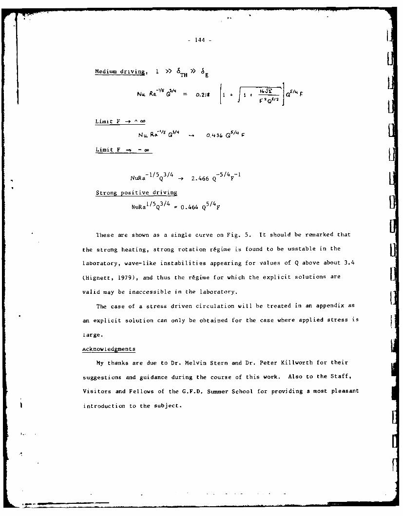
144-

Medium driving, 1 >> )TH >> E

N, k.I QI = 0.219 [ 4 1 1(Qr /

Limit F - +

'/S0.434?4u.Po G~Z I -I o.q34 Qs/"F

LimitF - -o,

NuRa-1/5 Q3/4 -2.466 Q-5/4 F-I

Strong positive driving

NuRal/5Q 3 /4 = 0.464 Q5/4F

These are shown as a single curve on Fig. 5. It should be remarked that

the strong heating, strong rotation regime is found to be unstable in the

laboratory, wave-like instabilities appearing for values of Q above about 3.4

(Hignett, 1979), and thus the r6gime for which the explicit solutions are

valid may be inaccessible in the laboratory.

The case of a stress driven circulation will be treated in an appendix as

an explicit solution can only be obtained for the case where applied stress is

Large.

acknowiedgments

My thanks are due to Dr. Melvin Stern and Dr. Peter Killworth for their

suggestions and guidance during the course of this work. Also to the Staff,

Visitors and Fellows of the G.F.D. Summer School for providing a most pleasant

introduction to the subject.

* "--

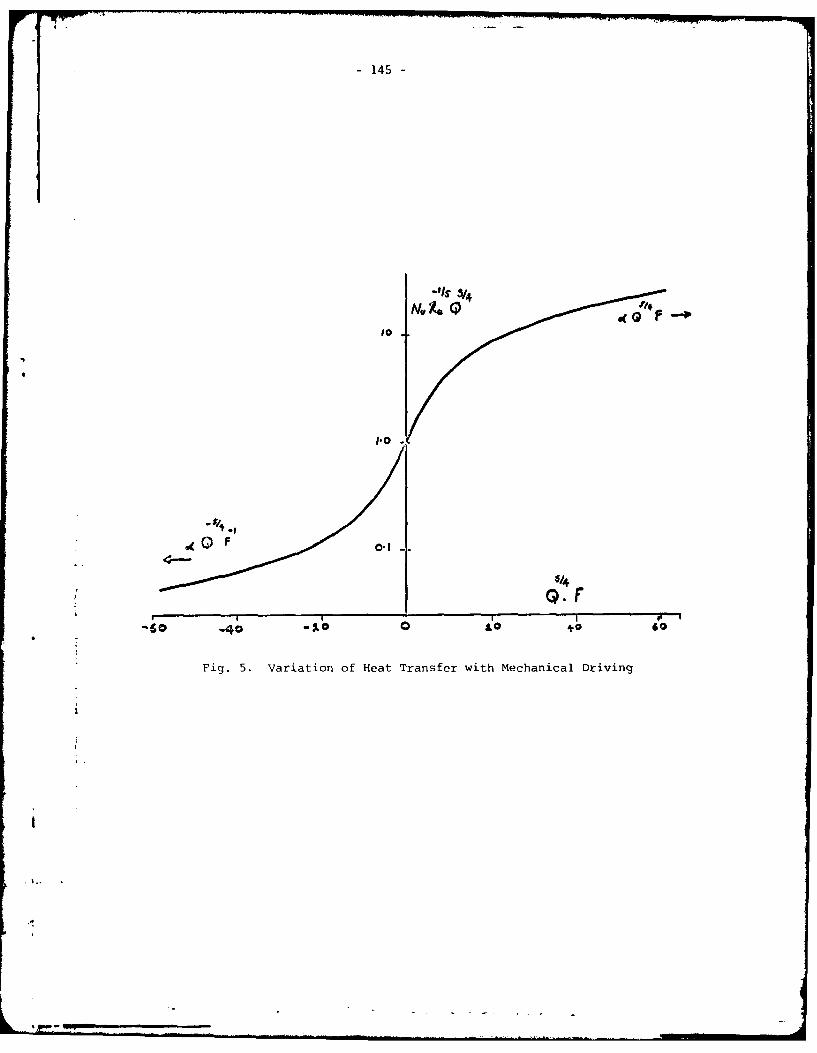
-145-

I-0

(0

6F

Fig. 5. Variation of Heat Transfer with Mechanical Driving

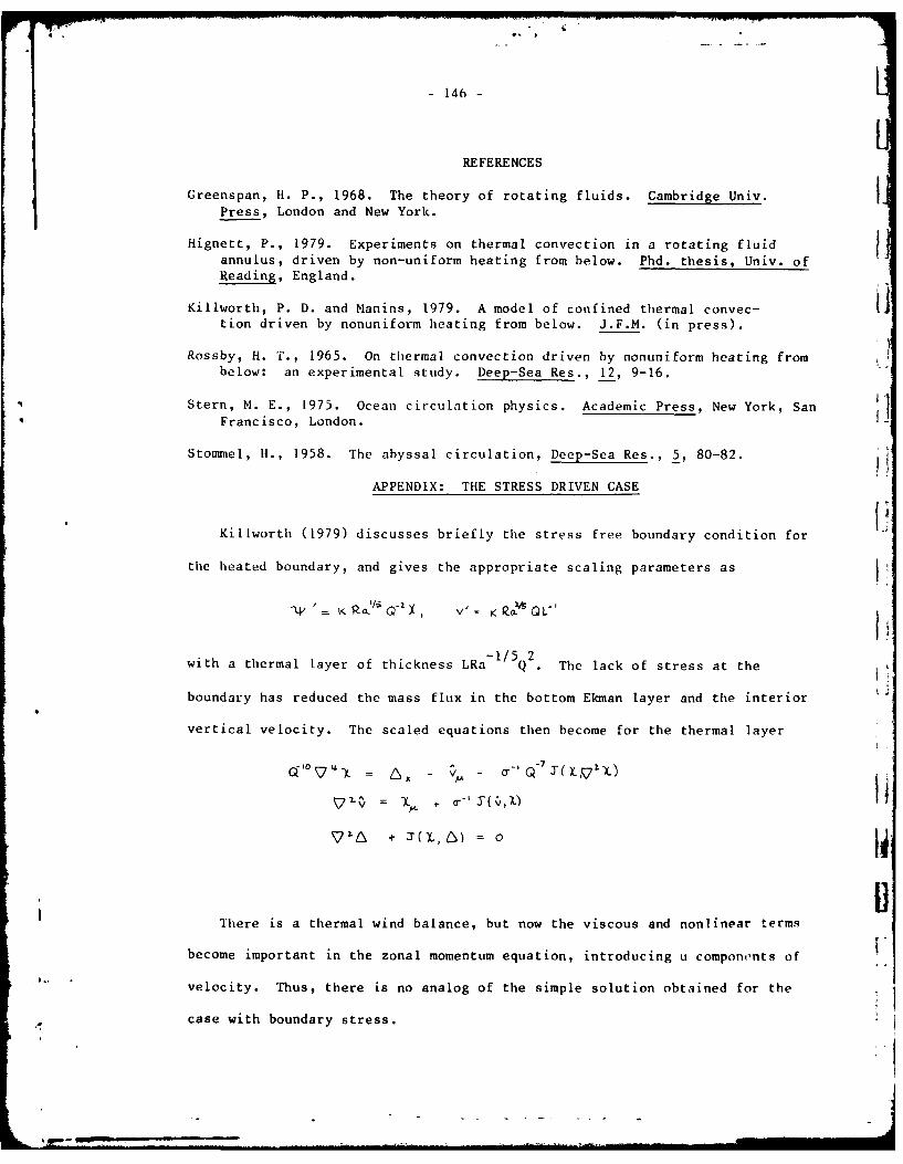
- 146 -

REFERENCES

Greenspan, H. P., 1968. The theory of rotating fluids. Cambridge Univ.Press, London and New York.

Hignett, P., 1979. Experiments on thermal convection in a rotating fluidannulus, driven by non-uniform heating from below. Phd. thesis, Univ. ofReading, England.

Killworth, P. D. and Manins, 1979. A model of confined thermal convec- ition driven by nonuniform heating from below. J.F.M. (in press).

Rossby, H. T., 1965. On thermal convection driven by nonuniform heating frombelow: an experimental study. Deep-Sea Res., 12, 9-16.

Stern, M. E., [975. Ocean circulation physics. Academic Press, New York, San

Francisco, London.

Stommel, H1., 1958. The abyssal circulation, Deep-Sea Res., 5, 80-82.

APPENDIX: THE STRESS DRIVEN CASE

Killworth (1979) discusses briefly the stress free boundary condition for

the heated boundary, and gives the appropriate scaling parameters as

'= KR&'Q - v'= 0 _'V

-1/5 2

with a thermal layer of thickness LRa Q . The lack of stress at the

boundary has reduced the mass flux in the bottom Ekman layer and the interior

vertical velocity. The scaled equations then become for the thermal layer

V 2-V^ = yX,. T--' J(. , I)

There is a thermal wind balance, but now the viscous and nonlinear terms

become important in the zonal momentum equation, introducing u compone'nts of

*' velocity. Thus, there is no analog of the simple solution obtained for the

case with boundary stress.

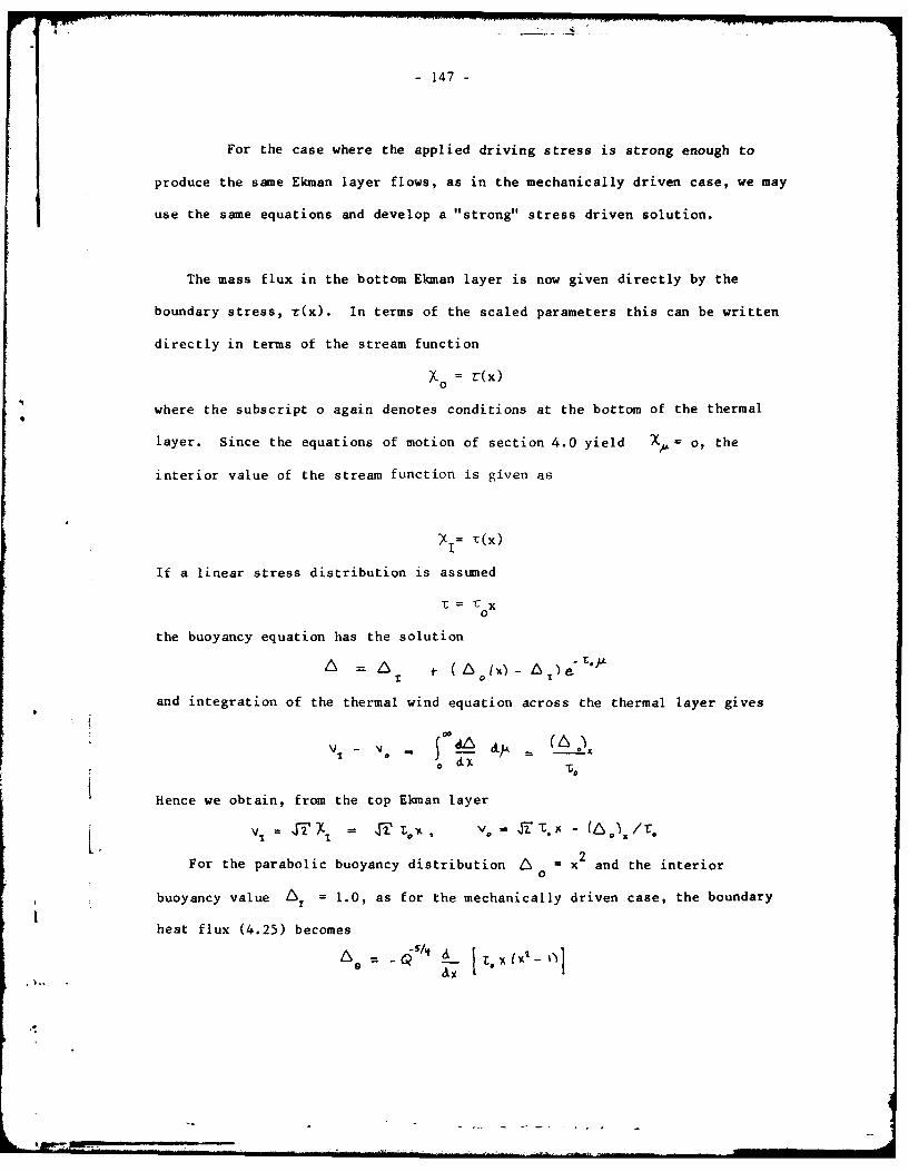
147 -

For the case where the applied driving stress is strong enough to

produce the same Ekman layer flows, as in the mechanically driven case, we may

use the same equations and develop a "strong" stress driven solution.

The mass flux in the bottom Ekman layer is now given directly by the

boundary stress, r(x). In terms of the scaled parameters this can be written

directly in terms of the stream function

) o = r(x)

where the subscript o again denotes conditions at the bottom of the thermal

layer. Since the equations of motion of section 4.0 yield X",= o, the

interior value of the stream function is given as

1i= t(x)

If a linear stress distribution is assumed

C= 7CX0

the buoyancy equation has the solution

and integration of the thermal wind equation across the thermal layer gives

Hence we obtain, from the top Ekman layer

1 T =' 1~ 7 T. A~ (,!S -

For the parabolic buoyancy distribution n = x2 and the interior0

buoyancy value 6r = 1.0, as for the mechanically driven case, the boundaryt

heat flux (4.25) becomes

S&... ,

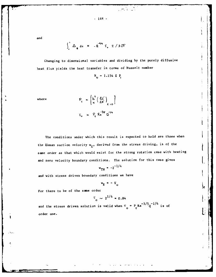
4. '" . -...... .. . . ....

148- I

and

S. ~r. ZC Z3'

Changing to dimensional variables and dividing by the purely diffusive

heat flux yields the heat transfer in terms of Nusselt number

N = 1.234 E Pu r

where 1 7

The conditions under which this result is expected to hold are those when

the Ekman suction velocity WE, derived from the stress driving, is of the I

same order as that which would exist for the strong rotation case with heating

and zero velocity boundary conditions. The solution for this case gives

- 1/4wTH '-2

and with stress driven boundary conditions we have

WE = - to° i

For there to be of the sane order

ro 21/4 = 0.84 3

and the stress driven solution is valid when T = P Ra Q is of

order one.

1., .|

- 149 -

CYCLING POLYNYA STATES IN THE ANTARCTIC

Douglas G. Martinson

1. Introduction

A remarkable feature of the winter sea ice distribution in the Weddell Sea

is the presence of an irregularly occurring polynya. This is a rather unexpec-

ted presence as it appears during periods of winter cooling in the center of

an otherwise ice covered region. It is important to understand this feature

as it might also be expected to have a moderating effect on the local heat

flux which substantially increases in areas of open water.

The polynya is a large C 106km2 ) open water feature which contains

as much as 15% ice and occurs quasi-periodically in the winters near the south-

eastern limits of the Weddell Sea (approximately 650S, 0°E). On a gross

scale the polynya appears to be present for three years, then missing for

three. This suggested cycle is based on an extremely short satellite record

relative to the cycling time and on scattered observational data. This paperFwill address three major questions pertaining to the polynya: I) Why does it

occur? 2) Why is its occurrence quasiperiodic (as opposed to full time) and

3) why does it always seem to occur in the vicinity of approximately 650S,

O°E?

2. The Theory

Most ideas concerning the origin of the polynya attribute its exis-

tence to the upwelling of warm deep water as it was assumed to form at the cen-

ter of a cyclonic gyre system where upwelling would be maximum. This appears

not to be the case, however, as shown by the wind driven circulation scheme of

Gordon, Martinson and Taylor (in press) which shows the gyre center

- 150 -

to be almost 100 north of the usual polynya position (Fig. I).

ii

I * i

Fig. 1. Streamlines representing cyclonic flow in Weddell-Ender'by basins.Maximum upwelling occurs in gyre center east of 300E. Maud Rise

Ii

is seamount located at 650s, 0OW (Gordon, Martinson and Taylor,in press). L

Corresponding Ekman upwelling values clearly show the maximum upwelling to

occur to the north and east of the polynya area (Gordon, 1979).

In light of the above results an alternative theory has been put forth by

Gordon (oral communication). The theory suggests that a preconditioning is

required which would raise the pycnocline and hence bring the deep water close

to the surface. Here it can respond to upper layer buoyancy changes due to

atmospheric cooling or salt ejection during ice formation. When the upper

layers become as dense as the deep water, overturning will occur and the warm,

salty deep water will mix with the cold, fresh surface layer. The large

- 151 -

volume of deep water will dominate the overturned temperature and salinity

characteristics resulting in warm, salty water which will then melt the ice

and form the polynya. A fresh water input at the surface (see section 4) would

then slowly stabilize the system again and the process repeats itself.

A likely candidate for the preconditioning is Maud Rise, a seamount located

at 65 S, 0 E (Fig. 1) over which a portion of the polynya always seems to

occur. Maud Rise comes to within 600 m of the surface and geologically is rich

in diatomaceous ooze (vs. clay ooze in the surrounding sediments), possibly sug-

gesting the polynya has been located in this same position over geological

time.

3. The Model

For the purpose of modelling, the system has been simplified to two levels

in the vertical with nonhorizontal variations. The vicinity of the polynya

appears to be an exceptionally good location for two level approximations as

can be seen by the Sigma-t vs. depth profiles in the belt from 650-70 °S and

0 -400W (Fig. 2). The approximation has several other advantages. By

using two distinct levels with averaged characteristics the effects of a

steady state upwelling will be incorporated into the model (through either the

thickness chosen for the upper level or the temperature of the upper level)

and the dynamics and cause of the preconditioning can be ignored as its

effects will also be incorporated into the levels.

We chose an upper level depth of 200 m for several reasons. First, 200 m

is a good approximation to the observations - at least in summertime. Second,

in a continuously stratified model of cooling near the polynya region, Kill-

worth (1979) showed that overturning almost invariably took place after mixing

had reached 195-200 m. Of course, in times of summer heating, a thin surface

mixed layer would form, with a depth determined presumably by Monin-Obukhov

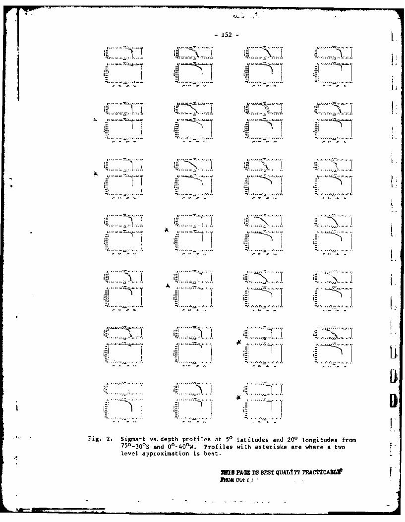
- 152 -

*.,~~~~~~ .. ../ ... ,....... .. ... .. . -.-. -j - --

... ... .. ....

I ; i ,- -V ' .. ." ...

Ilk,

' .....T-- ,- -- } r l" 4-. ... '.....! ,...... 1..... .... .. --, . . .

i. 2.SgatvIet rflsa 0 aiue n 0 ogtdsfo

' 0.-..3.. 0S a : ...-W. Piles - ' with asteiks arewhe"e-- .two-. M- .. - I_.- IS Q. I T A .- ...

-A..m _ I.. .... , .... ... . .... 1 ...... ,,._ .

: : ....." - --I] T -

*:i..............................-' ,- .

- - 1:1 -...

m, ~~~~.. *' .. ..'..'....

1...•'""Fig. 2. Sigma-t VS. depth profiles at 50 latitudes and 200 longitudes from75 -30S and O-40W, Profiles with asterisks are where a two "level approximation is best.

MI ?AJ 4ES ULT ~C'~Al~

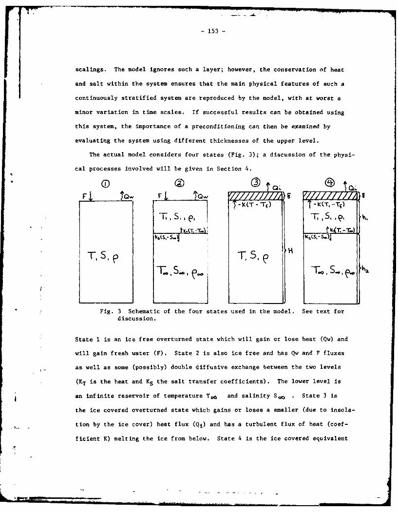
153

scalings. The model ignores such a layer; however, the conservation of heat

and salt within the system ensures that the main physical features of such a

continuously stratified system are reproduced by the model, with at worst a

minor variation in time scales. If successful results can be obtained using

this system, the importance of a preconditioning can then be examined by

evaluating the system using different thicknesses of the upper level.

The actual model considers four states (Fig. 3); a discussion of the physi-

cal processes involved will be given in Section 4.

'0

' ~M -i-K Tj) (-T, -Tq

t,T,-T.! _ Ik(s,- S., S

T S' T ,5T.,S.,'. ,

Fig. 3 Schematic of the four states used in the model. See text fordiscussion.

State 1 is an ice free overturned state which will gain or lose heat (Qw) and

will gain fresh water (F). State 2 is also ice free and has Qw and F fluxes

as well as some (possibly) double diffusive exchange between the two levels

(KT is the heat and KS the salt transfer coefficients). The lower level is

an infinite reservoir of temperature TQ and salinity SO . State 3 is

the ice covered overturned state which gains or loses a smaller (due to insola-

tion by the ice cover) heat flux (Qi) and has a turbulent flux of heat (coef-

ficient K) melting the ice from below. State 4 is the ice covered equivalent

.4|

- 154 -

of state 2.

The corresponding governing equations are as follows:

State I.

la"

qC

lb A

State 2

2a )

2b Y'

2c

State 3a-r-Ti -r; )

3 NHat - __" _-_-

3a

3bN~: o

3c C)Fa Y- K(-

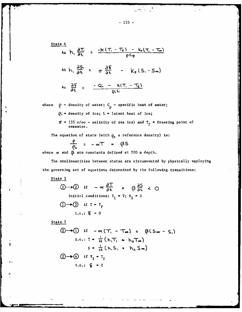
-155-

State 4

4a V, 4) - eT.

a t -

C- - a~ - ks(T , - )

where - density of water; C = specific heat of water;~p

• : density of ice; L = latent heat of ice;6" - (35 o/oo - salinity of sea ice) and Tf . freezing point of

seawater.

The equation of state (with a reference density) is:2- Z T @S

le.

where c and are constants defined at 200 m depth.

The nonlinearities between states are circumvented by physically employing

the governing set of equations determined by the following transitions:

State 1

if - O- + 0initial conditions: TI T; S1 S

if T = Tf

i.c.: 0 0

State 2

if -s

i.c.: T- -

Ir

if Tm1 Tf

i.c.: 0

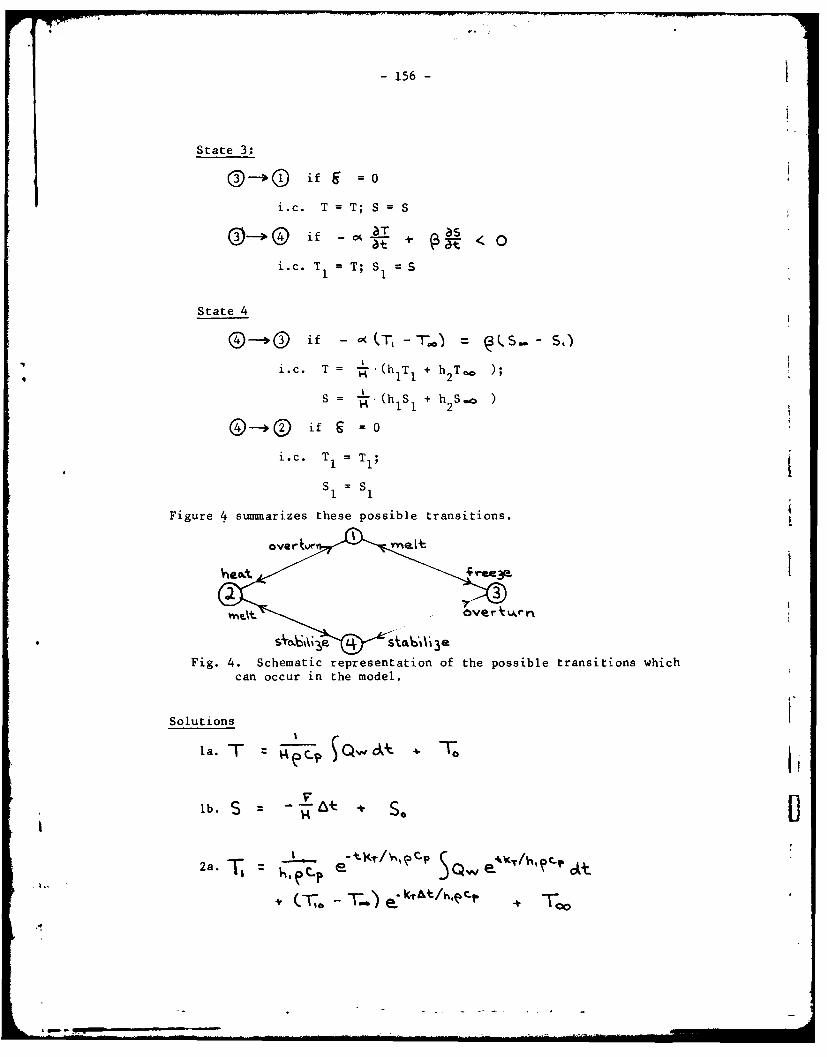
-156-

State 3:

@ if = 0

i.c. T T; S = S

at

i.c. T= T; S1 S

State 4

@ @ if - (I I T, CS,S,

i.c. T = - .(hiT I + h2T . )

S = -'-(hlS I + h 2S.0 )

@-'- @ if IF: 0

i.c. T = TI;

SI = S1, 1

Figure 4 summarizes these possible transitions.

overtv

nKt ".. _ ..--- -Ovrtr

*eAr $*b%3 £. S4.aatV-- 3 eFig. 4. Schematic representation of the possible transitions which

can occur in the model.

Solutions

lb. S + s So

2a. T C P QW P"/ " " At

* i (T. - T.) e TO

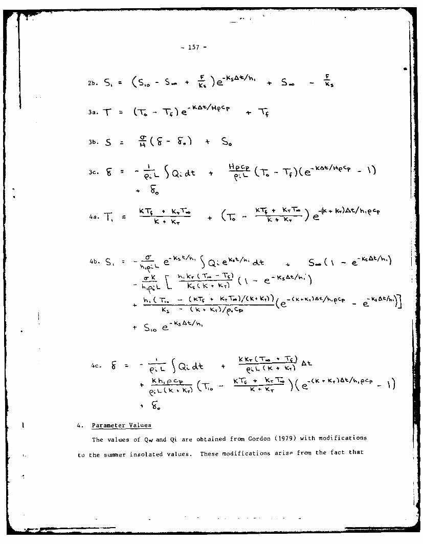
- 157 -

2b. S , = S- 4 I S . -z

3a. T - T+ &"+

3b. S C.3,

3c (v, Ot L ~ -7f) ( e -". .4 P c

4 a . T , = ( +-, , K ., e.

4b. ,- e k s t P / C e - V

(,C-r,. - ( KT; K., , V,)l~ p e VKt) ?

+ e_

4. Parameter Values

The values of Qw and Qi are obtained from Gordon (1979) with modifications

to the summer insolated values. These modifications arisp from the fact that

....... -_

-158-

Gordon's Qi summer values are for dry, white reflecting ice. In nature, as Q

changes its sign to positive the upper surrace of the ice begins to melt,

making a thin surface layer of water or wet ice. The result is a rapid de-

crease in the effect of the albedo and hence the modified values for summer

are the same as the summer Qw values. The actual value is probably some com-

promise between the two extremes. This modification of Q is necesary, to pre-

vent year round ice cover in the event of no overturning as the ice generated

during tke winter could not melt during summer using the white reflecting ice

values (Gordon, 1979, GFD, Lecture 2).

The value of K (turblent heat flux transfer coefficient into the ice from

the water) is taken from Killworth (1979) in which he derives a value of 2.59

x 103 cal/cm 2oC day. Values of Too and S.0 are taken from observa-

tions and are 00C and 34.66 o/oo respectively. The initial values of T1

and S (the computations begins in state 4 on first day of May) are also from

observations for May first and equal -l.9°and 34.40 o/oo respectively. The ice

is just beginning to grow so 6 = 0. Values for eL , L, a- and Tf are

taken from KilLworth (1979) and are .9 g/cm 3 , 60 cal/g, 30 o/oo and -1.9° 0

respectively.

The values of KT and KS are more difficult to obtain and of the two

methods used to derive their values here, agreement is only within an order of

magnitude. The first method from which KT can be derived represents an upper

limit. Assuming no overturning, one can set KT at tile value necessary to

balance the yearly loss of heat from the upper level. When solving for KT ,

in this manner a value of 6 cal/cm2 °C day is obtained. Alternatively,

KT can be solved for by constructing a seasonal ice cycle. For the ice to

disappear by the beginning of summner, as is usually observed, an

- 159 -

overturning must occur at the end of spring. Working backwards from here and

using an iterative approach a seasonal cycle can be constructed (see section

5) in which KT is considered the only unknown. In this manner, for various

values of F, the value of KT is 0(0) in these units. The actual value of

KT used for most of the results presented here is 6 cal/cm 2 oC day.

Sensitivity of the equations to these parameters is discussed in a later

section. KS is in all cases taken to be 15% of K as suggested by Turner

(oral communication).

The input of fresh water into the system is essential to the model. As can

be easily seen, with no fresh water entering the overturned state the high sa-

linity would persist and each year following the summer heating cycle, over-

turning would occur as soon as the temperature of the upper level cooled to

ToO .The fresh water flux required to stabilize the system can enter it in

two ways. Precipitation is an obvious source. Estimates of precipitation over

evaporation for this area are of the order of 50 cm/yr.

Another possible source of F arises from the fact that in years when a

polynya occurs there is essentially a 10 3Km 3 volume of ice not formed which

normally acts as a fresh water sink. If one assumes that the ice (or some

fraction of it) which frequently forms in the polynya area melts elsewhere

than in polynya years, no ice forming would represent a fresh water input. An

upper limit for this case (assuming all the ice melts elsewhere) is approxi-

K_ mately 100 cm/year for polynya years (and 0 for the nonpolynya years).

In this model F is converted to a fresh water flux (50 cm/yr _- 4.9 o/oo

cm/day) and is input to the system only during periods of open water.

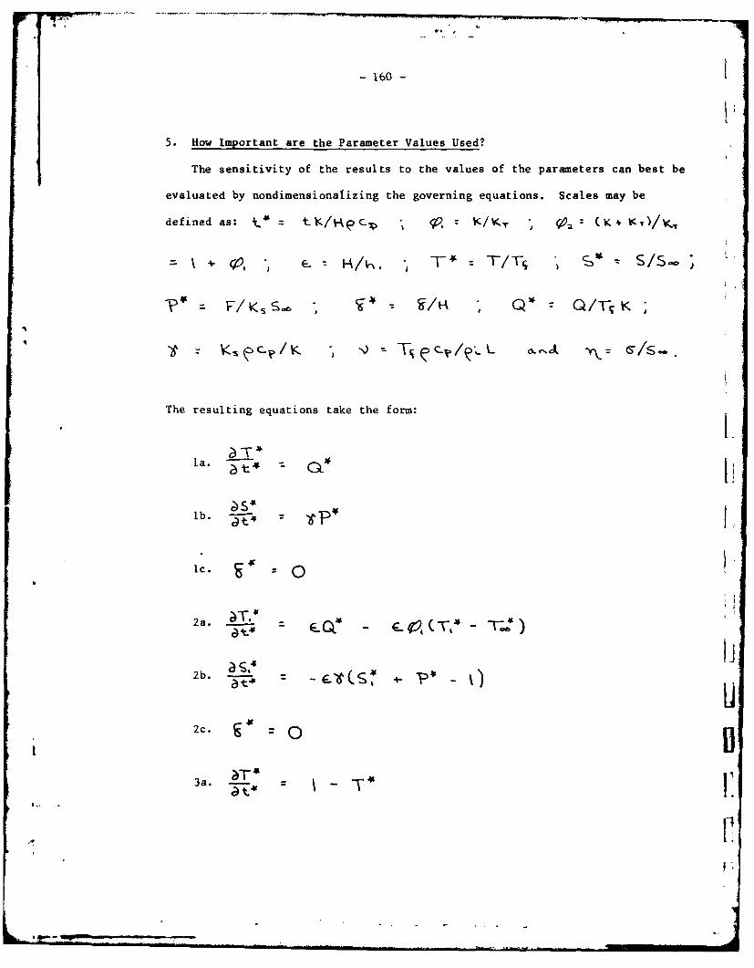
-160-

5. How Important are the Parameter Values Used?

The sensitivity of the results to the values of the parameters can best be

evaluated by nondimensionalizing the governing equations. Scales may be

defined as: = tK/t- 9 c . " /4- , 4a: ( K 4 KK)/,.

/- K, -TS. , Ss, ,

Y" e - , Tsc ?~L o.& -

The resulting equations take the form:

la. t C"

lb. a t VP*

lc. 0

2a. -L'Z

C) 44 ev(T* -r.4)

i

2b. ()

2c. E (=0

3a. 41[

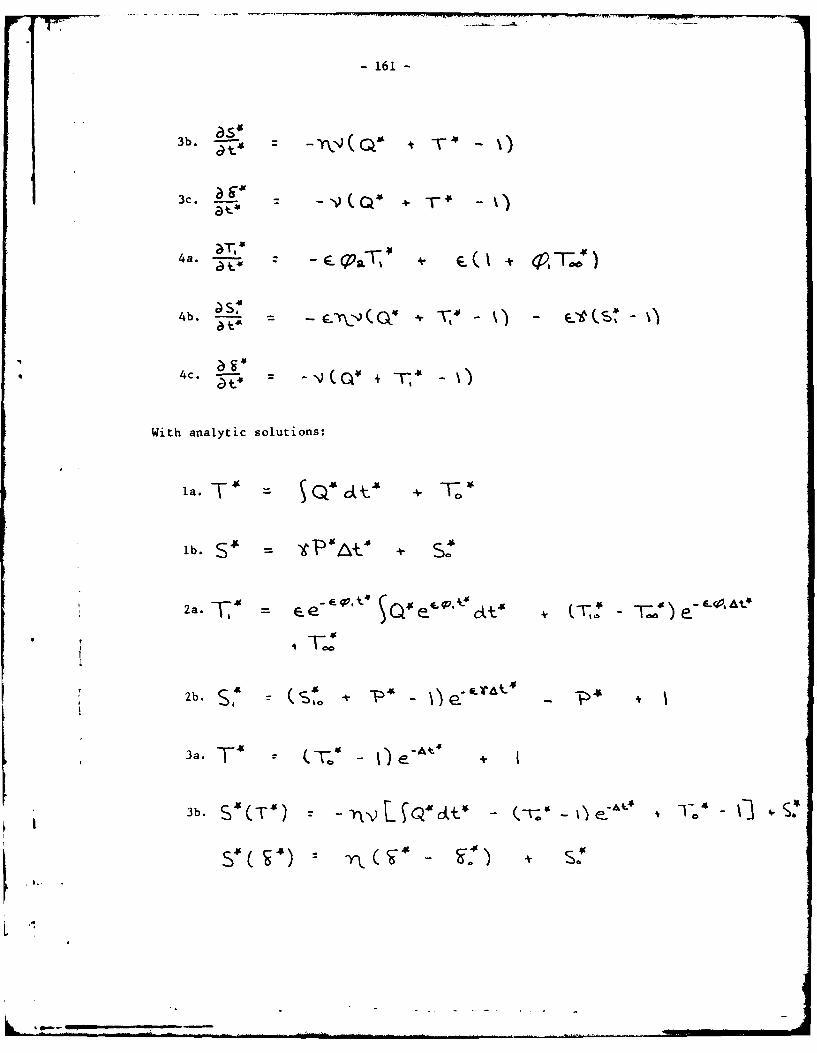
- 161 -

3b. s * -

3c. + T-a! 4 -(Q T" - )

4 aT - i 6 * -T:64

4b. -S- v (S-'

4c. )t- +

With analytic solutions:

Ia.4 TT,

lb. S* + S!

2a. T --e QE qw, t-

2b. Ss +~ -

3a. T(T - -At +S t

T A3b. S'(' _qa" -.- To-- S;

,* 41 S

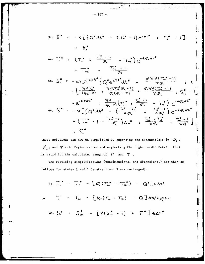
-162- L

i.i

3c. T'I: OW , - I

-4a T -

-

4b , e-". ' - -U.e 1%. - n T - "q \*!

4b. e - - - -y C7 -C .V t er

+ $- M Ti,

These solutions can now be simplified by expanding the exponentials in I I .;,and '" into Taylor series and neglecting the higher order terms. This

is valid for the calculated range of , and '

The resulting simplifications (nondimensional and dimensional) are then as

foltows for states 2 and 4 (states 1 and 3 are unchanged): I.T

4c. - \q ri -- &]At I

o .r T" = , - l c,"- TI - ]I,,=an r- intoSTaylor - and o -t.n -highr /or e. Ti

f l fstae 2 -4 (s I a 3 a

X T 4 7 42 T, %i

- 163 -

or So - iK S - S. o Y/

4a. (T, ( 1 - - e +

or e -

4b.= -y(T'.)1~ 1 !)- Y" Th' \ -Z

4b.5 -oiE (TO4 4t - -T+ TO -

4tO~

~This reduces state 2 solutions to simple linear functions and state 4 solu-

• tions reduce to exponentials with time scales of the order of 10 days in K.

l Comparing this to KT time scales of the order of 10,000 days in state 4 and

~two orders of magnitude less than the Qw term in state 2 suggests that the

effects of KT are essentially negligible. The effects of the diffusive

transfer of salt (Ks), however, is not neglibile as So- =

r~ ~ ~ (s1o Vs1 vI )

0(1/5).

, The effects of the other parameters can best be seen by examining their

effects on the slopes and time scales for the various states on a T-S diagram

which evolves with Lime (Fig. 5).

_1-- - - L ( T ,, .,-...e-

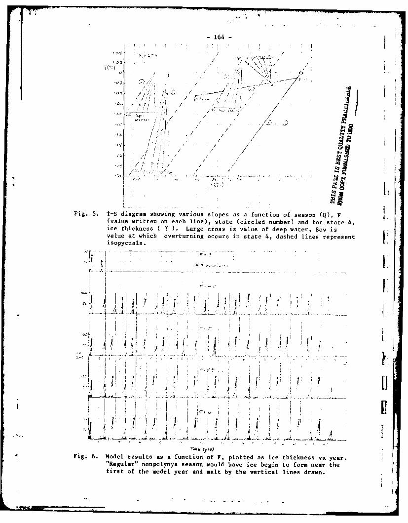
164 -

*02 .

*01 t. , / a,

/ /- 5 5. /I./. .... / .- r,

-o+ ... :: ,., " ---- "' : 7 , /J... i

" / f , ce thi- / .

valu a-S7t hich ovrtrnn ocur in stt ,dahdlnsersn

/ /// /

-II' / / .1 /

q, .,, ..'-I

j .: . I .. ... :__ -_

IfI

• ~~~~~~~~~~~~- . .;,"i. .. /................ ... ............ L ,

Fig. 5. diagram showing various slopes as a function of season (Q), F L(value written on each line), state (circled number) and for state 4,ice thickness ( * ). Large cross is value of deep water, Soy is

value at which overturning occurs in state 4, dashed lines represent

isopycnaIs.

F ..*. .'-& .----.-_. -.. - -:.._i "-. .... . .. .-- .. . . ." . 't..

* 1 , ' ii ijj ': 4-

ii i, ij ' 4 A . , , !,

* .... ~7a lt Cyi!s

.4 ig.6. ode reult asa fncton f F pltte as ithkesv.ya.

"Rglr nnoyy seso o lhv ic bei tofr na hfis fth oe ya n melt by-th vrica line drwn

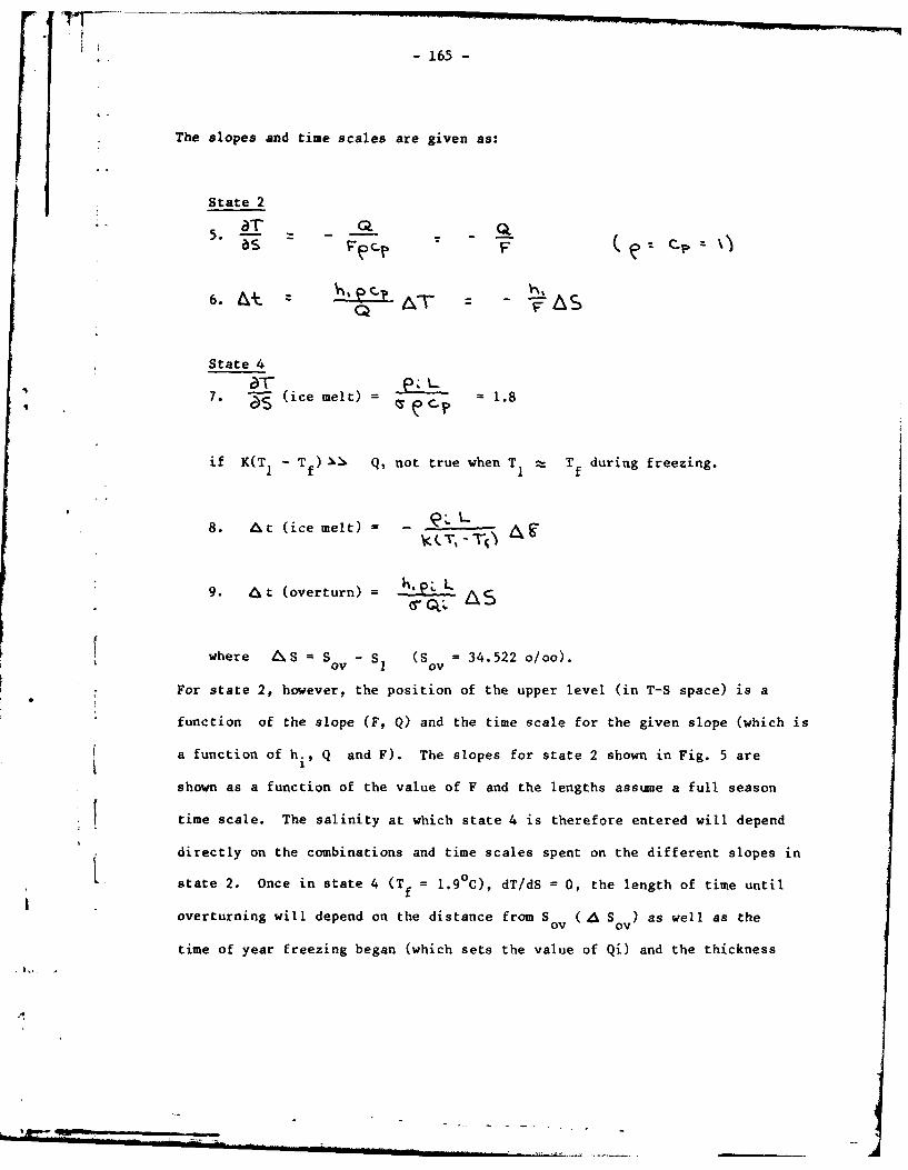
-165-

The slopes and time scales are given as:

State 2

5. T - Q

6. AT -S

State 4

7. (ice melt) - 1.8

if K(TI - T ) Q, not true when T r Tf during freezing.

8. At (ice melt) = - L L.I TI - TO &

9. At (overturn) = .p. L

where S - Soy - SI (So f 34.522 o/oo).

For state 2, however, the position of the upper level (in T-S space) is a

function of the slope (F, Q) and the time scale for the given slope (which is

a function of hi, Q and F). The slopes for state 2 shown in Fig. 5 are

shown as a function of the value of F and the lengths assume a full season

time scale. The salinity at which state 4 is therefore entered will depend

directly on the combinations and time scales spent on the different slopes in

L state 2. Once in state 4 (Tf = 1.90C), dT/dS = 0, the length of time untilIf

overturning will depend on the distance from S (At S ) as well as the

time of year freezing began (which sets the value of Qi) and the thickness

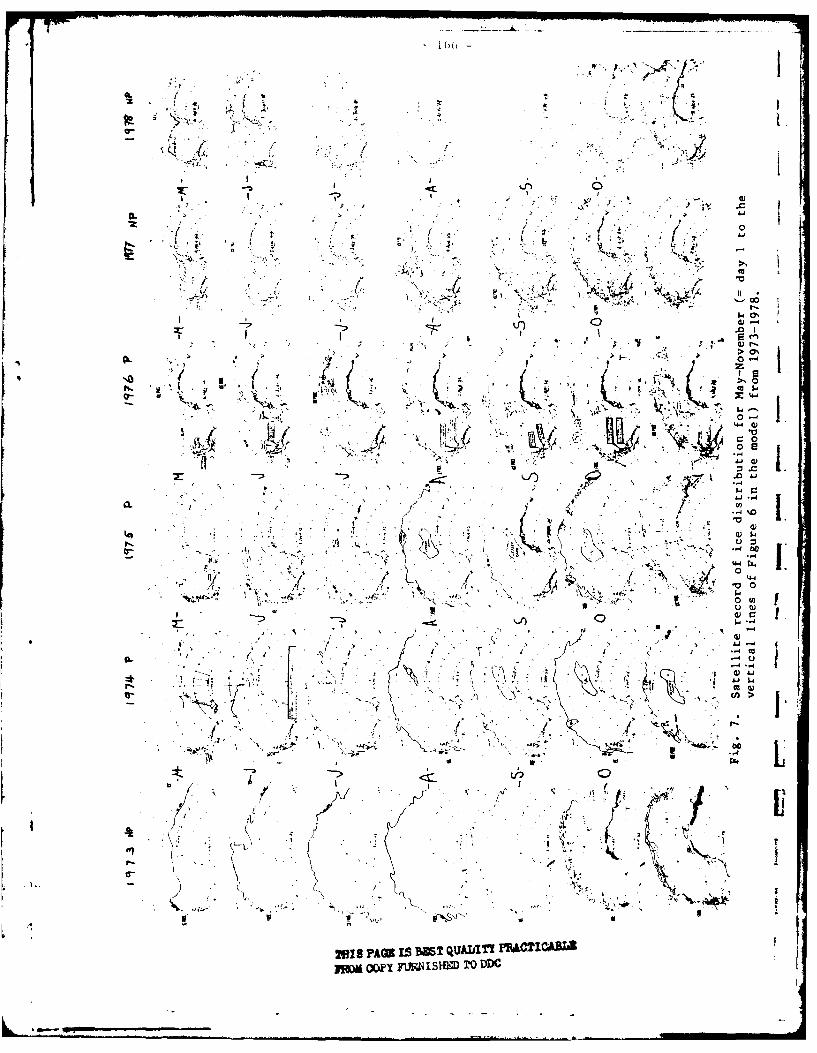
S. ON

f -4I S 0

*~~~~ 0 ~K 1' -i

r... -4

- 0

4,-t t t~I

IS I P A IS B M 5%L

-167

assumed for the upper level (h ).If overturning occurs the slope in T-S

space during melting is constant, but the distance down the slope depends on

the amount of ice melted. If overturning does not occur, the melting ice will

simply return to the position on the T f line at which state 4 began and the

effects of summer heating and subsequent fall cooling back to the freezing

point will result in a net decrease in salinity. The new freezing period will

therefore have to produce more ice before overturning and the ice melt slope

will then increase reiative to the prior overturned year.

From this it can be seen that the resulting T-S position after each change

in Q is very sensitive to the values of F, Q and h. A slight change in the

length of time on a slope directly affects the positions of the following

slopes which may cause overturning to occur earlier or not at all.

6. Model Results

The model results for various values of F are given in Fig. 6 as plots of

ice vs. time with the first of each year corresponding to the first of May.

Figure 7 shows ice conditions (from satellite images) for the months of May -

t November from 1973 - 1978. It can be seen that for values of F -4 3 the fresh

water input is too low to overcome the high salinity resulting from over-

turning.

This is easiest seen in Figure 8a which shows that after the ice melts

following year 2 the slopes in state 2 are not shallow enough (due to low F)

to move to a position of low salinity; hence, when ice forms in year three

only a few centimeters are necessary before overturning. The ice melt slope

is then barely traveled and any cooling now results in almost immediate over-

turning. The slopes in state 2 are too steep for the system to ever recover

and hence ice never forms again.

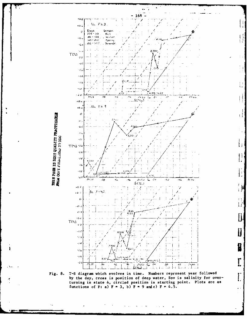
- 168-

TCO 4~ / .07

3 .0 j , . . ,

LI: ;- i . .; ¢, , / / "; .IIlrj 9 -

00

,' / I /./ : - -:. .. . / " " r /.... - " - .0 - .•

,./ /./ __ . . I *a, _._g /

, j / .3'/

L I/

.8 / .... Numbe. ; y followed

-.a // , -- ,' , ' - .. , . .. ..

b d," cros i o / t , i " f

turningi , i /

state 4 c r l . . . Plots. a r a

func. .. ... .of ' a F - • F 9 ' F 4 ..'/ , L " I" .... /"[

" " ": : : .. ./ ; k i .. .. '. : i . . . ..." " "

,: • / : '. '/" . .

.,o; : / .I. , / : / 1-

-/., .. .. . . ./ . " " : .. . : ' ..... - :- 9

F i ...- d i a g r a w h i c I , I. .. . . . ..

Fig.8. -S iagrm wichevolves in time. Numbers represent year followed

by the day, cross is position of deep water, Soy is salinity for over-

turning in state 4, circled position is startng pont. Plots are as

functions of F: a) F =3, b) F =9 anc) F - 4.5.

-. .: . -

-169-

F values of 5.5 to 9 result in overturning every other year with the only

differences in the results being the amount of ice built up and the seasonal

extent of the ice cover. For F =5.5 overturning occurs in August at which

time a polynya would form whereas for F = 6 the overturning occurs almost a

month later.

For values of F > 9 the system receives too much fresh water input and

the upper level quickly becomes too stable for overturning (Fig. 8b). In this

case the slopes are so shallow that the position on the T-S diagram is toward

low salinities very rapidly and eventually not enough ice can form in the

cooling seaon to overcome the fresh water input.

Values of 4.5 - 5 for F (see Fig. 8c) seem to result in an irregular

cycling where polynas form at various times of the year and some years not at

all. Comparing the results of these two cases with the observed seasonal ice

distribution (Fig. 7) reveals many striking similarities. The previously

considered "regular cycle" is now observed as being irregular. Overturning

is seen to occur at different times each year and as late as August (1979),

October (1973) and November (1978). This is reproduced in the model results

as is an irregular cycle in the time when the ice begins to form (compare ice

growth for August 1973 with August 1977). Another result from the model is

that years in which a polynya forms are often followed by years of late ice

formation and thin ice thickness. This is seen in the data by examining the

1977 season, which follows the full polynya of 1976. Ice growth does not

cover the region of the polynya until as late as July with an aereal extent

which is much smaller than years of full polynyas like 1974 and 1975. Whether

the ice was as thick as 1977, however, is unknown. The model also shows a

high number of years in which overturning occurs at some time before the end

L . amp

-170-[

of the normal ice season. Previous examinations of the data had only con-

sidered such years as 1974-76 as overturning polynya years and the other years

as non overturning. In light of the model results, however, it can be seen

that in the last six years (including 1979) overturning has occurred before

summer in five of them (vs. four of six years in the model results).

Finally, because the data show that overturning occurs (e.g. October

1973), it lends support to the model's use of a large discontinuity in the

equation of state which preconditions overturning as opposed to a continual

thickening of an upper layer with no overturning.

7. Sensitivity to Varying Parameters

The model has been tested for the effects of natural variations in the

parameters of Q and F. This has been done in a variety of ways which includes Ithe following:

1) Shocking the systt--. The values of Q were increased and decreased by

10% on the twelfth yea.- of the run for the entire twelfth year. The values of

Q were then increased, decreased and alternatively increased, decreased every

fourth year of the run by 10%. These tests were then done to F and finally to

both Q and F.

2) Stochastic variation. The values of Q were changed daily stochastically

by as much as ± 20% for the entire 25-year run. This was then done to F and[

finally to both Q and F together.

3) Stochastic variation and shocking the system. The final testing was Ivarious combinations of the previous tests concluding with a run which

included all the perturbations on both Q and F together.

The purpose of perturbing the system was to subject the model to various

* perturbations which might be expected in nature (a suggestion of a four-year

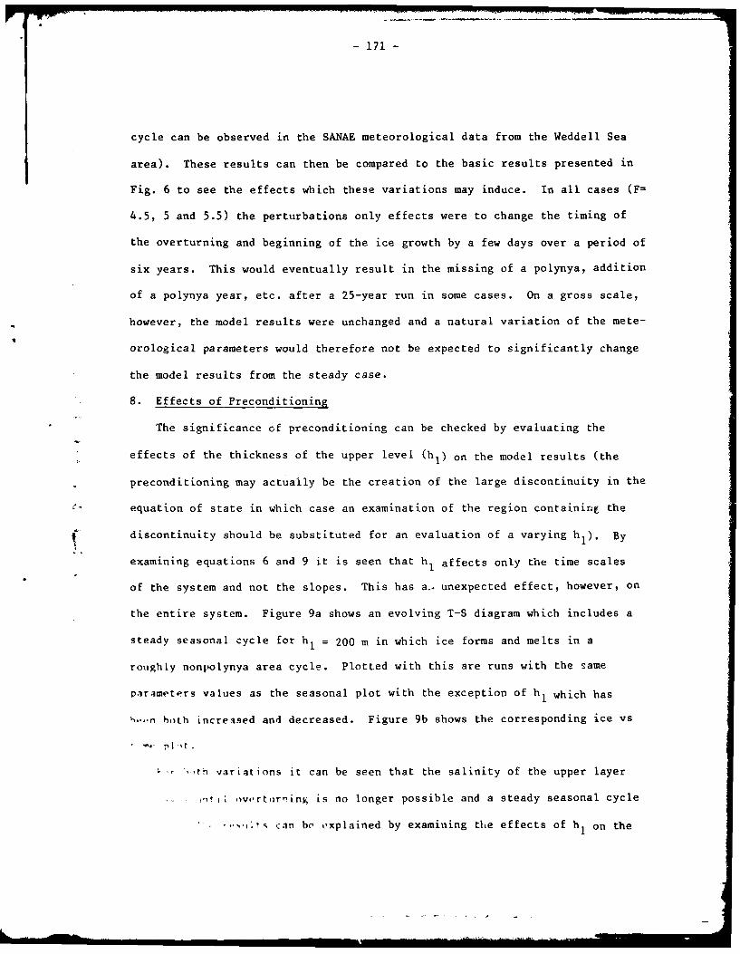
-171-

cycle can be observed in the SANAE meteorological data from the Weddell Sea

area). These results can then be compared to the basic results presented in

Fig. 6 to see the effects which these variations may induce. In all cases (F=

4.5, 5 and 5.5) the perturbations only effects were to change the timing of

the overturning and beginning of the ice growth by a few days over a period of

six years. This would eventually result in the missing of a polynya, addition

of a polynya year, etc. after a 25-year run in some cases. On a gross scale,

however, the model results were unchanged and a natural variation of the mete-

orological parameters would therefore not be expected to significantly change

the model results from the steady case.

8. Effects of Preconditioning

The significance of preconditioning can be checked by evaluating the

effects of the thickness of the upper level (hl) on the model results (the

preconditioning may actually be the creation of the large discontinuity in the

equation of state in which case an examination of the region containinr the

discontinuity should be substituted for an evaluation of a varying hi). By

examining equations 6 and 9 it is seen that hl affects only the time scales

of the system and not the slopes. This has a . unexpected effect, however, on

the entire system. Figure 9a shows an evolving T-S diagram which includes a

steady seasonal cycle for hl = 200 m in which ice forms and melts in a

roughly nonpolynya area cycle. Plotted with this are runs with the same

parameters values as the seasonal plot with the exception of h i which has

.... n both increised and decreased. Figure 9b shows the corresponding ice vs

* -. ' 1.',t.

6- ,t h variations it can be seen that the salinity of the upper layer

inil ovrturiing is no longer possible and a steady seasonal cycle

". .. 1 can be explained by examining the effects of h i on the

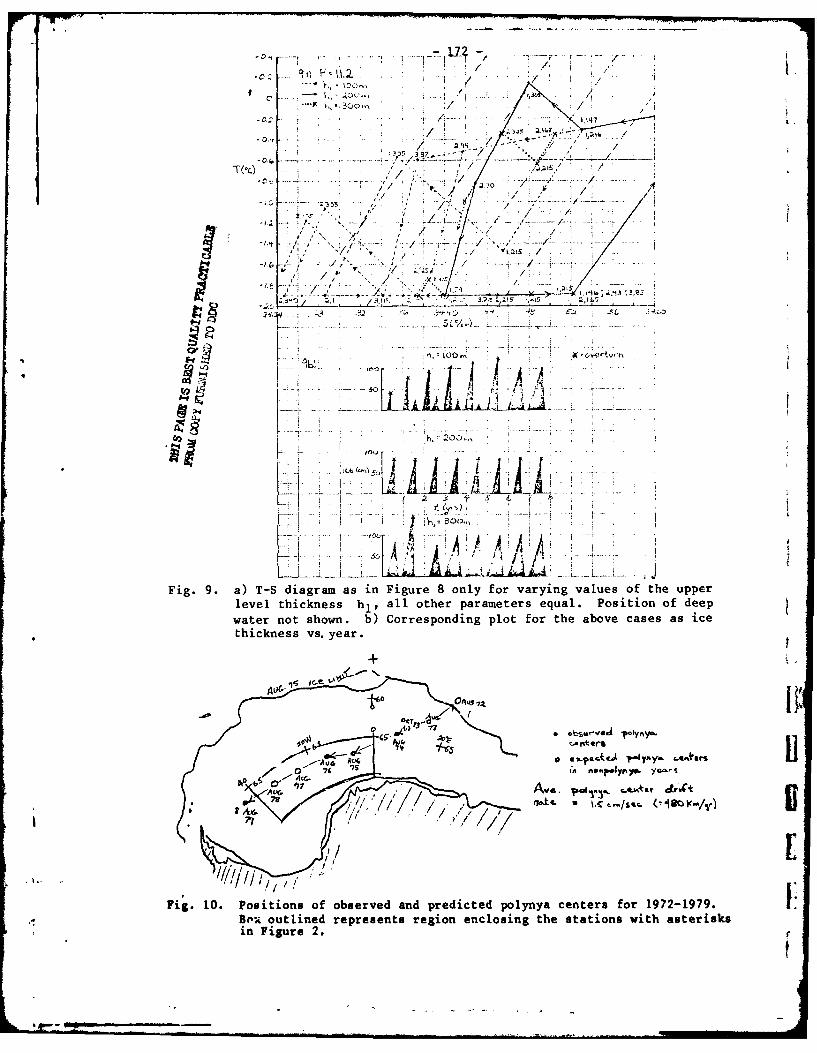
N-2.

-50

N 03

W

L6/Fig. 9.a - iga s i iue8ol frvrigvluso h pe

AA- -)5 _AAZ..iAA.....thicnes vs. year

o~ 0,tt AtG.Y

Fig. 10. Positions of observed and predicted polynya centers for 1972-1979.

Be% outlined represents region enclosing the stations with asterisksin Figure 2.

-173-

time scale. In state 2 a reduction of hi by one-half has the same effect as

doubling F, although the time scale is now also halved before freezing will

occur. Therefore the same amount of fresh water as usual should enter the

system. During the freezing cycle, however, overturning will occur twice as

fast and there is then a period of winter which is normally ice covered which

will be receiving (at its increased rate) an input of F. The net effect over

the year is to receive a much higher input of F. This F is persistent and not

removed by overturning because after overturning there is still enough

cooling left for late spring ice formation. Summer heating removes this ice

and during the remaining summer and fall cooling more F is input resulting in

lower salinity and m~ore ice formation needed until overturning. The effects

therefore of increasing F is not removed as more F is being stored in the

larger volume of ice. The salinity decreases yearly until overturning is no

longer possible.

Increasing of 11h slows the response time and decreases the effects of F

in the equations. In this case, however, the same amount of ice formation as

f for smaller hi is not enough to overturn the system and more ice is required.

-The time scale of ice formation has not been affected by varying h 1so the

* system does not overturn until late in the season. The overturned water is

now very warm and after the summer heating requires too much of the cooling

cycle to refreeze. By the time it does start to form ice there is not enough

cooling season left to generate the ice necessary for overturning. Therefore

the effects of F have not been compensated and the upper layer slowly becomes

fresher until overturning is impossible.

-174- V

It can therefore be concluded that the effects of preconditioning are

important. It is also interesting to note that in Fig. 10 the polynya which

has formed during the time at which this paper was being written is not in the

vicinity of Maud Rise but is in the belt previously mentioned. The implica-

tions of this have not been evaluated as yet, but it is worthy of mention that

the polynya center appears to be drifting westward at the same rate as the

mean calculated current of 1.5 cm/sec from their 1974 position over Maud Rise.

9. Conclusion

The model at this stage seems to contain the necessary basic physics

required to simulate a quasi-periodic polynya situation. It would also appear

to offer plausible answers to the three questions originally addressed. These

are as follows:

1) The polynya occurs because of haline induced overturning due to the

ejection of salt during ice buildup into a preconditioned upper level. This

also suggests that there will be more ice production during polyna years.

2) The polynya occurs quasi-periodically because of the sensitive nature

of the time scales on the various slopes on the T-S diagrams, especially for

particular ranges of fresh water input. Some slight variation may also occur

due to the variability of Q and F in nature.

3) Finally, the polynya occurs in the belt in which it has been observed

because of a preconditioning responsible for positioning the depth of the

surface layer at the position in which it is most susceptible to overturning

for the amount of fresh water entering the system.

* 1..

- 175 -

Acknowledgements

The author is extremely indebted to the entire GFD Staff and Fellows for

helpful discussions, comments and suggestions. In particular thanks are due

P. D. Killworth, who offered continual assistance and ideas. Also A. L.

Gordon, G. Veronis and M. E. Stern contributed much in the way of ideas and

suggestions which were incorporated into the paper.

REFERENCES

Gordon, A. L., 1979. Meridional heat and salt Flox in the Southern Ocean, GFDLecture 2.

Gordon, A. L., D. G. Martinson and H. Taylor, 1979. Wind driven circulationof the Weddell Gyre, in press.

KilLworth, P. D., 1979. On chimney formation in the ocean. Jour. Phys.Oceanogr., 531-544.

.4

-176-

EXPERIMENT WITH DOUBLE DIFFUSIVE INTRUSIONS IN A ROTATING SYSTEML

Bert Rudels

Introduction

It is well established that the difference in the molecular diffusivities

for heat and salt (or any other solutes) may create gravitational

instabilities and convection in a stably stratified fluid (Stern, 1975;

Turner, 1973). These instabilities most likely play an important part in the

mixing and transformation of water masses in the ocean.

In the last couple of years experimental and theoretical work have been

devoted to the effect of horizontal variations of heat and salt concentra-

tions. Double diffusive intrusions have been studied (Turner, 1977). Corn-

pared to a nondiffusive intrusion the most striking effect is the much larger

volume of fluid affected by the intrusion. Layers are -reated which move into

the surrounding fluid driven by horizontal pressure gradients set up by the

double diffusive convection. Because the greater mass flux across a "finger"

interface compared to a "diffusive" interface the density changes in the [layers and the flow will be across isopycnals. These effects may be ofr

importance in frontal regions of the ocean where large lateral variations of

salinity and temperature occur.

Works with double diffusive systems in a rotating frame, however, have

been scanty. The experiments described below were initiated by some pre-

liminary runs done by Stewart Turner at GFD earlier this simmer, using salta

and sugar. Some of these experiments showed a large-scale instability dis-

rupting the intrusion. The experiments, in a crude way simulate an oceanic

vortex. If instabilities occur due to double diffusion, the destruction of

oceanic vortices may be enhanced. It is therefore important to explore the I

-177-

evolution of the intrusion and the conditions favorable for instability. To

accomplish this has been the aim of this work..

Experiments

A. Introduction

The work was done in the laboratory in Walsh Cottage. A square tank

38x38 cm was used and the fluid height was approximately 20 cm in each run. The

experiments were done using salt CT) and sug-ar CS). A linear density gradient

was set up by stirring a two-layer system with a screen while rotating, after

9 which the density was measured at three levels, 15 cm, 10 cm, and 5 cm with a

densiometer and the density gradient was computed. This method of creating a

linear gradient seemed to work surprisingly well. Moreover, by using the grid

the spin-up time could be reduced considerably. The injection was always at

its own density level and kept as close to the center (vertically and horizon-

tally) as possible. Because of the difficulty of making measurements while the

experiments were running the main work was done by varying the initial para-

meters:

-ItBasic density stratification 0.001 < L~ < 0.oo63cm

Density of the intrusion +' PS4 p' i. o, 1. 0, 1. 0 C

where p.is the density due to sugar in the intrusion

Rotation rate 0. - o~S < < 2.o 10.C:.

- 178 -

Total amount of injected fluid = Q(4' 'I

The rate of flow was kept fairly constant at a rate of 1.5 ml/min.

The evolution of the quantities listed below were measured from

photographs taken during the experiment:

R = radius of the well defined central core

h = height of the well defined central core

Rl= maximum radius of intrusion

H = height of the convecting salt finger region above the central

core

The flow profile was qualitatively explored by dropping dye into the tank.

The main object of study, however, was the occurrence and evolution of the in-

stability as a function of the initial conditions. A total of 29 runs were

recorded in this way. Most of the experiments were with sugar solution in-

jected into a salt stratification but some experiments (6) were done by injec-

ting salt into sugar.

B. Description

I) Control

An injection without double diffusion will create motion in the

system. Since the fluid is injected at the center it has no angular momentum

and it will therefore start spinning anticyclonally as it is moving outwards.

Also, because the density surfaces will be compressed above and below the

intrusion, the whole fluid will gain relative negative vorticity. LA control experiment with salt into salt, for instance, was

necesary. This experiment showed a stable perfectly axisymmetrical disc. Theneeay

iIb~.

.4!

-179-

vertical cross section seemed to be deviating slightly from a perfect ellip-

soid and the radius was increasing faster than the Rossby radius computed from

the amount of injected fluid. This more rapid increase may be due to viscous

effects which slow down the zonal velocity of the disc and make it spread

faster. The importance of viscosity was apparent because the relative angu-

lar velocity decreased rather than increased with distance from the source, as

it would if only conservation of angular momentum was taken into account.

2) Experiments with Double Diffusion

a) Basic Features

When double diffusion was present the nature of the intrusion

changed markedly. Because of the convection the vertical extent of the region

affected by the intrusion was greatly increased. It was still possible, except

in extremely unstable cases, to observed a V4ell defined central core. This

central core was assumed to represent the size and shape of the injected

fluid and distinguished from the ambient fluid affected by the diffusive pro-

cesses. When no instabilities were observed the central core had a distinct

ellipsoid form. Above and below this core a large region of fluid was trans-

formed by the double diffusive convection. The depth of this region was

greater at the side of the salt fingers (we use the term salt fingers even if

sugar fingers would be a more correct term to use in these experiments) where

it assumed a cylindrical or flattened dome shape. The much shallower

penetration on the "diffusive" side was terminated with a horizontal "dif-

fusive" interface with roughly the same width as the core. More than one

interface could be present in the vertical. Layering was also observed on the

"finger" side. The number of layers was markedly lower and appeared to be

more horizontal (when stable) than in the nonrotating case. The presence of

-180-

salt fingers greatly increases the exchange of momentum between the injected

fluid and its surroundings, thereby distributing the added negative angular

momentum over a larger volume, making it spin anticyclonally as a whole.

Velocities were largest near the center of the tank, and decreased outwards.

In this general anticyclonal flow there were regions where relative cyclonal

flow was present. In cases where instability occurred, this cyclonal flow was

stronger than the basic rotation having absolute cyclonal velocity.

b) The Instability

Apart from the regions of increased cyclonal zonal velocity, two

features were distinct when the intrusion became unstable.

1) The instability occurred near the center of the intrusion and

appeared like thrown out arms. These arms usually formed one by one, but in

some cases when the salt was injected into sugar, they occurred in pairs.

When moving outwards the arms roughly kept their aximuthal

position, indicating that regions with cyclonal velocity were thrown out.

This belief was strengthened by the fact that the tip of the arms sometimes

changed into vortices with weak but positive vorticity.

2) The whole intrusion seemed to become twisted vertically, giving

the intrusion a beautiful helical shape. The twisting seemed to occur more

than once, creating a number of intertwining helices, making the appearance of

the intrusion more and more chaotic with time.

An observational connection between the arms and the helices

could not be made for certain. In the most unstable cases the central core

was totally disrupted and only the "halo" created by the diffusion could be

seen.

- 181 -

Organization of Observations

The experiments indicated that the instability occurred most easily for

low rotation rates and low stability, and for high concentration of the

injected solute 5, CT) (differences in concentrations should be used if the

injected solute is present in the ambient fluid).

In diagrams I and 2 the occurrence of instability is shown on a Tplane

where N = 1 !q is the Brunt Vaisala frequency, kept

constant. Diagram 3 shows the experiments on a p'/f -plane for constant

density stratification.

The dependence upon ps and was expected, but the stabilizing

effect of the rotation was rather surprising. These matters will be discussed

further below.

To be able to order the observations we introduce the concept of an ideal

intrusion. This intrusion is at each instant (each Q() ) at its Rossby

radius and we then have by definition

Q = Cl).,t

"IAZ,

L . i

) T~ (assumirg cylindrical shape)

which gives I'

, (2)

=[GO V3L- Z.

L *.

-182-

By forming and we can then compare the evolution of the central

core as a function of Q(+) with this ideal case.

From the diagrams it can be seen that the observed radius is greater

than R? for large OC+) and the difference increases with Q

The opposite is true of the observed height ' which is less than k and,

here too the difference increases with a

These observations seem to indicate that volume is roughly conserved

within the core and corresponds to the amount of injected fluid. The

differences 9-R-Z T - sT may be due to the changing density in the

core and the changed density gradient in the convecting region which would

give a different theoretical value of the Rossby radius This cannot be the

explanation for the salt injected into salt case which sl ws the \ame

features. Here the difference is most probably due to vis us eff ts. The

disc is slowed down and then spreads out faster. The shap so devates from 1an ellipsoid which may explain whaolume does not seem t e conserved in

this. case 4.0"1 is measuref at the center).

Diagm S shows , the maximum horizonta radius of the intru-

si pn compar d to the Rossby radius. As expected, R I is uch larger

tan £, I and the difference increases with Q ( . As a whole the

o4servations show great scatter, especially at the sta of each experiment

(fmall 0 ), but they becqme less scattered with i reasing Q

To get a vertical scale H1 of the convecting r ion, which compares Lw.th its observed vertical extent H , we make th following idealiza-

tions of the double-diffusive,!convection.

.4J

- 183 -

Fig. 1. Salt solution is injected, at its own density level, into a linear

salt gradient

p'= 1.100 g/cm 3, & = 0.002 g/cm 4, f = 0.80s-1

Black tape on pipe - 2 cm. (The same on all figures)

Fig. 2. Sugar solution is injected, at its own density level into a linear

salt stratification.

* = 1.100 g/cm 2 , - 0.002 g/cm4, No rotation.

MCM

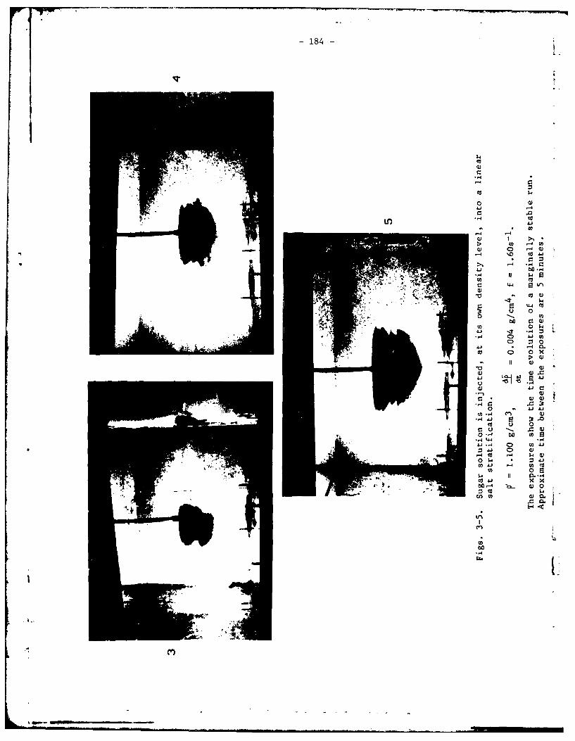
-184-

$4

4 D cc

cu $

o c

C . l.

,3

-4 4 -84 J

03 4J

- d - pu w0 4 $4

co 41 o t

U) 03

o 4 I1 -

SI

' '-4 0 '

AD-AO 45 WOODS HOLE OCEANOGRAPHIC INSTITUTION MASS F . /8199 SUMMER STUDY PROGRAM IN GEOPHYSICAL FLUID DYNAMICS Ar THE --ETC(U)NOV 79 M E STERN, F K MELLOR NOOlN-79-C-0671

UNCLASSIFIED WHOI-79g-8-VOL-2 NL3. 1 ,EIBEEEBBEhE .EE.EE

EHEEHEHELIII

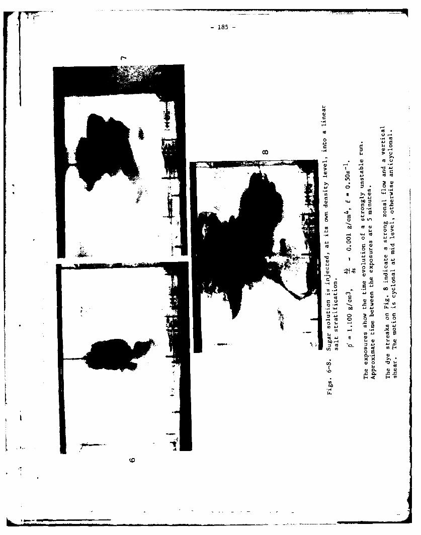
-185-

C)o

Luu

-) 4 -4 -

0) (JA ca

'.4 * O

44-I I-

4 4-i

0 m cAr A*

s, 0 3 0

ew 4' 0 ) 0n "

0 0~ >u-

1-4 44 CO )C 0 4.J -4

0 CO -

00

H-4 CO 4JI -40

-4~ 41 cuS 4-1 -

elk 3-t -4

$O4 4 0) rCI412U (0 ) o'1

W *4 14 0* XX >1

o

C0 .G

0

>44

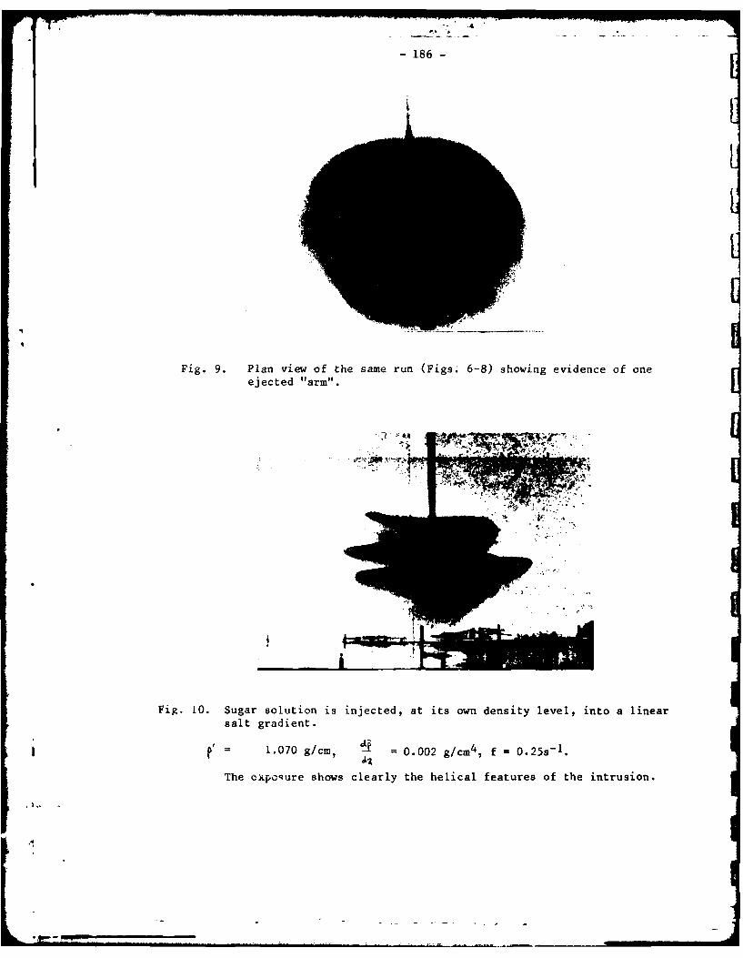
- 186 -

q

Fig. 9. Plan view of the same run (Figs. 6-8) showing evidence of oneejected "arm".

Fig. 0. Sugar solution is injected, at its own density level, into a linearsalt gradient.

'= 1.070 g/cm, _ = 0.002 g/cm 4 , f = 0.25s-1.

The exposure shows clearly the helical features of the intrusion.

Mp -4

-187-

a) Only the mass transport carried by the fingers is considered important.

b) All e. in the intrusion is exchanged for pT with the ambient

fluid. The flux F. of sugar can be estimated from the relation F. - (P,)

K ; 10-2 cm2sec-l found by Stern and Turner (1969). We

find that the fingers are capable of transporting the injected amount of sugar

into the surrounding fluid during the time of an experimental run ( -30

minutes). For the mass flux M between the intrusion and the ambient fluid the

relation M = 4'k, holds. A 'is the change of density in the intrusion.

9c) The ratio F T F sbetween the fluxes of salt and sugar is 0.9 (Stern

and Turner, 1969). Using this value the density change in the intrusion can

*be written as

F= At FS fsAtJ [0.9 Pi.1 - r,1]=0.1s

Note that the sign of L depends upon if salt or sugar is injected. In

(a) and (b) we have neglected the concentration changes in the ambient fluid.

*If these are taken into account, the total exchange would be less by a factor

o fh H

d) There is no radial variation of the diffusion. This should be

justified when the lateral scale of the intrusion is small, that is, for

large T' and small

*(e) All release of buoyancy by the fingers is used to rearrange the

*density field from a linear gradient into a step profile. This is a dangerous

assumption because of the high viscosity of the fingers.

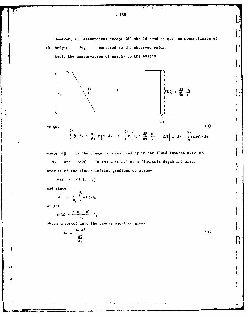
-188- U

However, all assumptions except (d) should tend to give an overestimate of

the height 'HI compared to the observed value.

Apply the conservation of energy to the system

P.

+z 2

we get (3)

where A is the change of mean density in the fluid between zero and

H? and .(2) is the vertical mass flux/unit depth and area.

Because of the linear initial gradient we assume

and since

n. S.(z CZH.

we get

HI,

which inserted into the energy equation gives

4C 4)

dZ

L

1....

189 -

since we have

- = - O.I rHT

we may write H, as a function of the initial conditions

T= -1(5)

The expression shows that H . increases slower with Q than RT and hT.

We see that H T is an overestimate of the convecting region H as

it should be, but the difference H-H diminishes when f and AF I

become large. This is the case when (d) becomes most violated. The other

assumptions do not depend upon variations of these quantities so they should

be as good or as bad for all f and _ . The variation with Q(t) isdT

not as great as the diagram seems to indicate. Instead H - H, tends to

approach a constant value when Q becomes large. For the most part the

scatter is due to variation of initial parameters especially f and suggesting

that the functional dependence of these parameters given by (5) is not quite

correct in describing the evolution of depth of the convecting region.

Qualitative Criteria for Instability

Because of double diffusion the whole volume of the intrusion has become a

center of high relative vorticity. The strength of this vorticity ;

should be compared to the basic vorticity P . To find 4/f we need

to get an estimate of the zonal flow induced by the change in the density

* .*

-190-

field. We will assume a geostropically balanced flow

-v 1 p(ignoring the term ) (6)

and compute the pressure gradient due to the vertical mass flux. The vertical

mass flux per unit area that can be carried by the fingers is given by

M = )A = 0.1 ps6' = P

Here assumptions (a) and (b) above have been used. We may note that to get

the mass transport it is not necessary to assume anything about the amount of IAenergy being used to change the density profile. The pressure gradient is

then estimated by

and the zonal velocity becomesn

0. 1 P Z 0. 1 (v = (7)

when RT is expressed by the initial parameters. Surprisingly the zonal

velocity appears to be independent of the rotation rate. It was not possible

in the experiment to find if this actually was the case since other effects,

due to the injection of fluid and to the instability itself, prevented good

estimates. It seems, however, to agree with the observed fact that a low

rotation rate was destabilizing.

L

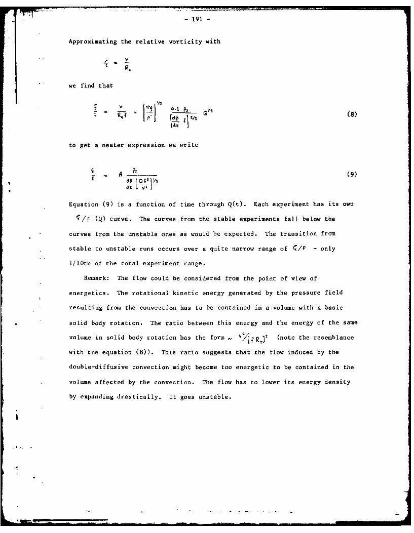
- 191 -

Approximating the relative vorticity with

we find that

V 0.1 fS (8)

Rj ;2/1

to get a neater expression we write

dzI 'Iq

Equation (9) is a function of time through Q(t). Each experiment has its own

/ (Q) curve. The curves from the stable experiments fall below the

curves from the unstable ones as would be expected. The transition from

stable to unstable runs occurs over a quite narrow range of a/f - only

1/10th of the total experiment range.

Remark: The flow could be considered from the point of view of

energetics. The rotational kinetic energy generated by the pressure field

resulting from the convection has to be contained in a volume with a basic

solid body rotation. The ratio between this energy and the energy of the same

volume in solid body rotation has the form - v2 (note the resemblance

with the equation (8)). This ratio suggests that the flow induced by the

double-diffusive convection might become too energetic to be contained in the

volume affected by the convection. The flow has to lower its energy density

by expanding drastically. It goes unstable.

.4

-192-

It is seen that the occurrence of instability is closely related to the

amount of relative vorticity generated by the diffusion (Diagram 8). We may

find by choosing Q the value q/f above which the intrusion is unstable. For

instance,

Q = 100, 4 - 3. 5

(The runs with salt injected into sugar seemed to give a higher value (Diagram

9). Too few runs were, however, made to establish this as a fact.)

The representation is not good because of its time dependence through Q.

A nondimensional representation can be given by plotting

versusT

for any particular Q.

The slope of the time dividing the stable from the instable experiments is

given by N-

and is constant for all Q. The position of the line, however, changes with

Discussion

a) The Instability

The intrusion is assumed to always keep its Rossby radius as it

iV

4-;

- 193 -

expands. The double diffusive convection changes the density of the intrusion

and the surrounding density field. The theoretical value of the Rossby radius

then increases and the intrusion has to adjust to keep up with the changes.

In some cases this adjustment is easily done and the disc grows gently to its

new size. In the unstable cases the change in Rossby radius is too great and

sudden. The central core is disrupted and expands violently to its new size.

This means that in experiments with a constant injection of fluid the strongly

unstable cases are never able to build up a stable central core but always

have to start anew, pass through the singular destabilizing phase, and get

disrupted.

The fact that the instability acts to increase the rate of expansion of

the intrusion seems to suggest a barotropic, or even centrifugal, type of

instability rather than a baroclinic one, even if the energy available to the

instability comes from the creation of a baroclinic density field.

b) Zonal Velocities and the Helical Shape

The whole region of the intrusion has an anticyclonal rotation due to

the injection of fluid with zero angular momentum. This angular momentum is

rapidly distributed over the convecting region because of the high viscosity

due to the salt fingers.

However, in addition to this the downward mass flux creates a low

pressure zone inside the convective region. A corresponding cyclonal flow is

then generated inside the general anticyclonic circulation. Because the

vorticity has to be conserved a corresponding anticyclonal flow must be

generated somewhere in the fluid. If the double diffusion redistributes

density in the vertical this anticyclonal flow may occur inside the convective

,,.

-194-

region. Otherwise a barotropic anticyclonal circulation must be generated in

the whole fluid. This may be done by a horizontal squashing of the diffusive

region which will raise the free surface and create a general anticyclonic

flow (Fig. 11 and 12).

The vertical shear, thus being present, acts upon the highly viscous

convective region. This region will then become twisted by the zonal flow,

somewhat like a bar twisted vertically, if the viscosity is strong enough. A

simple kinematic feature like this may help to explain the observed helical

shape of the convective region.

These thoughts must, however, remain highly speculative since not enough

is known about the nature of the flow inside the convective region or about

its interaction with the salt fingers. The helical shape can be generated in

an altogether different way, more closely related to the double-diffusive

mechanisms and the instability.

Conc lus ions

The experiments show that strong zonal motions, and even instabili-

ties may occur when an intrusion interacts with its environment through double

diffusive convection.

A general criteria for the occurrence of instability could not be found

because of the continuous increase of volume Q of the injected fluid.

however, the lines of marginal stability were seen to have the same slope for

all Q. The position of the time was shifted towards the origin with increased Q.

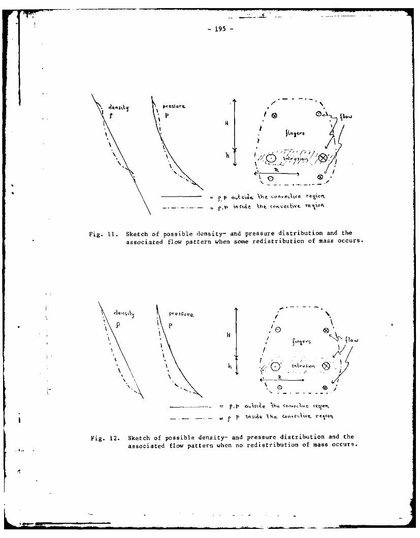
- 195 -

,..* . ".

-. CJ -- a -k, p is.s4 't% cn'erie_ reifL

Fig. 11. Sketch of possible density- and pressure distribution and the

associated flow pattern when some redistribution of mass occurs.

aetsik ~ 9r~v

5' 0

Fig. 12. Sketch of possible density- and pressure distribution and the

associated flow pattern when no redistribution of mass occurs.

.4

l |1 I li " -

-196- L

These experiments suggest ways in which the molecular effects may

influence motions on a Larger scale in the oceans. Cyclonal velocities .created by the downward mass flux may be present in the subsurface cyclonal

eddies that have been observed in the Arctic (Hunkins, 1974). These eddies

showed high cyclonal velocities connected with intrusions of anomalously cold

water.

The transformation and mixing of oceanic eddies can also be speeded up

considerably if these eddies become unstable and disrupt. Because of the lack

of field observations these thoughts should be regarded as speculations.

Acknowiedgements

I would like to thank Stewart Turner for introducing me to the experiment,

Melvin Stern tor his guidance during the work, Adrian Gill, Louis Howard, and

George Veronis for many discussions. Thanks is also due to Robert Frazel for

ail his help and to Florence Mellor and Maryanne Macaluso for their work with

the manuscript.

REFERENCES

hunkins, K. L., 1974. Subsurface eddies in the Arctic Ocean. Deep-Sea Res.,21, 1017-I033.

Stern, M. E., 1975. Ocean Circulation Physics. New York, Academic Press.

Stern, M. E. and J. S. Turner, 1969. Salt fingers and convecting layers.Deep-Sea Res., i6, 497-511.

Turner, J. S., 1973. Buoyancy effects in fluids. London, Cambridge Univ.Press.

Turner, J. S., 1978. Double-diffusive intrusions into a density gradient. IJour. Geophys. Res., 83, 2887-2901.

* [

- 197 -

BOUNDARY DENSITY CURRENTS OF UNIFORM

POTENTIAL VORTICITY

Bach-Lien Hua

Introduction

Oceanic examples of boundary density currents can be found in regions of

abyssal western boundary currents. Their time-dependent behavior is related

to the intermittent formation of cold water that sinks in wintertime to the

bottom of polar coastal regions (Wadhams, Gill and Linden, 1979). The struc-

ture of each current, their width and stability, are questions of great impor

tance since their temperature determines the mean temperature of the bottom of

the oceans. The same features, upside down can be found when fresh water from

coastal source debouches in a plume in saltier water. The effect of rotation

compensates late-al spreading due to buoyancy forces and constrains the light

water to flow along the coast in a confined current which is geostrophic behind

the nose of the intrusion.

The rate of propagation of the nose of the intrusion and some nonlinear

dynamics on the trailing geostrophic front have been examined by Stern (1979),

but with the restriction to flows of zero potential vorticity. Such flows

appear as the simplest generalization of nonrotating irrotational flows and a

possible realization is when the intrusion comes from an infinitely deep

reservoir (Whitehead, Leetma and Knox, 1974).

This summer's work is an extension of Stern's paper and considers flows of

finite potential vorticity, first for an intrusion overlying an infinitely

*deep layer at rest (Section III) and the interaction with the dynamics of a

second layer of finite depth is taken into account in the last section.

The equations describing such flows are complex and would require a

thorough numerical reduction. We have then chosen to concentrate our

attention on two main points:

1) Investigate if the result found by Stern (1979) that there exists a

limiting width of the boundary current for a bore-like steady intrusion

propagate, is still valid for finite potential vorticity flows in a two-layer

ocean and find numerically that value.

2) See qualitatively if some nonlinear waves found in Stern (1979) have

their analogs in our problem.

II. Experiments

Some qualitative experiments relevant to the above dynamics were conducted

with the set-up represented on Fig. 1. In a rotating channel, light fluid is

separated from a heavier one by a vertical barrier and the ensemble is brought

to a state of solid rotation. At initial time the barrier is pulled up. If

the channel was not rotating, light fluid would be raised buoyantly over the

heavier one and the flow would be uniform through the section. If the fluid

were rotating, but if there were no lateral walls, we would face the classical

problem of geostrophic adjustment. Because of the Coriolis force, the flow is 1parallel to the pressure gradient and the limit between light and heavy fluid

is displaced to the right (facing the flow) on a distance of a Rossby radius

of deformation. In this case, the presence of the lateral wall deviates the

light fluid in a boundary flow that is constrained by rotation to flow along

the right wall (looking downstream) in a confined current of width comparable

to the Rossby radius of deformation.

Some features observed in the experiments have been sketched on Fig. 1.

The flow presents a very complicated pattern just in the corner behind the

initial position of the barrier, where the flow of light fluid strikes the

lateral wall.L

Downstream of this very complex region, the intrusion appears to be

parallel, laminar and steady, upstream of the nose of the intrusion. The

*1

- 199 -

speed of propagation of the nose appears to be uniform in time and its shape

looks unchanged while it advances downstream.

The range of some parameters chosen for the experiments are

rotation range w = f/2 0.2 - 1G- 1

density difference 10- 3

Rossby radius of deformation 2.5 cm

width of the channel 15 cm

The lateral frictional boundary layer thickness in our experiments was

around I mm, so that the influence friction may be neglected on the boundary

current, except in the incipient frontal part of the intrusion. After some

time, certain experiments were unstable and finite amplitude wave patterns

could be seen on the trailing front behind the nose and some observed waves

would steepen and break towards the upstream direction and bumps in height and

width of the current, associated with those waves, would appear almost in

phase.

This experiment is the rotating analog of densimetric exchange flows in

rectangular channels (Barr, 1972). The analysis of the actual rotating

experiment is complicated by the possible influence of the other lateral wall

on the light fluid intrusion. However, we expect, as shown by Gill (1976),

that if the radius of deformation is small compared with the channel width, as

a first approximation, the influence of the other lateral wall may be neglec-

ted.

The existence of the frontal wall that ends the channel may also cause

reflection of surges at the interface between the two fluids once the density

current has reached the frontal wall. But the greatest complication in analy-

zing the experiment results from the region on the corner just behind the

initial position of the barrier, where a sort of complicated adjustment occurs

.,

- 200 -

and from which a laminar intrusion emerges. In this corner region, both

highly transient and short-wave effects occur, therefore, the following theory

cannot be taken into account. The situation, as idealized from the experiment,

may be applied to the laminar intrusion. The parallel flow behind the incipi-

ent nose will be referred to hereafter as the upstream state as opposed to the

nose itself. We then deal with a boundary current, constrained along a

straight coast, and presenting a density front.

One important premise is the conservation of potential vorticity in each

layer (both the intrusion layer and the bottom layer). This supposes that

changes in potential vorticity induced by mixing and friction may be neglected,

so that modelling by an ideal fluid can only be applied over limited path

lengths. Moreover, as in the experiment, we will restrict our attention to

initial distributions corresponding to uniform potential vorticity in both Jlayers, since at initial time both light and heavy fluids have uniform poten-

tial vorticity 1/Hi (i = 1,2) where H. is the initial height. (Experi-i I

ments were also conducted for H1 0 H 2' the heavier fluid having an L-

shaped distribution, lying on both sides of the barrier and on the bottom

beneath the light fluid, in the light fluid compartment.)

III. Density Current of Finite Potential Vorticity

1) Equations: We shall first consider the case of an intrusion overlying

an infinitely deep inactive ocean. If denotes the depth of the intrusion,

k designates the vertical axis, and f/2 is the angular velocity, the hydro-

static equations for the horizontal velocity V are:

t ( + ) kx V = " '(qR+ v1/z) (1)- o (2I

L e

- 201 -

where ' k - V x v is the relative vorticity. (1) and (2) imply that

~.fT 0 so that for a uniform potential vorticity distribution -w

this yields: 4 +

- adimensionalization:

We introduce the following nondimensional quantities:

v= H 0o

y (gH) 12f- 1

x~ 1 gH)1/2 -1• x = a- (gHo)0/f-]

1/2u = (gH)

0

1/2,v = C (gHo) 0

-1 -1It = E f t

H designates the height scale, and E is the ratio of the length scale in

( the y-direction over the length scale in x-direction.

Hereafter, the notation " denoting nondimensional quantities will be

omitted. The equations in nondimensional form are:

for x-momentum equation: (3)

for y-momentum equation: (4)

. +I

-202-

Ifor continuity equation: (5)

for vorticity equation: (6)

If L(x,t) denotes the nondimensional displacement of the front (h 0 0) from

the wall, the boundary conditions may be written as:

no normal flux at the wall:

v(x,O,t) = 0 (7)

The height goes to zero on the free streamline y = L(x,t).

h(x,L(x,t),t) = 0 (8)

Kinematic condition on the free streamline:

v(x,L(x,t),t) = dL (9) jdt

The height far upstream behind the nose is chosen to scale the heights in the

problem:

h(-oo,o,t) f 1 (10)

- straight boundary current:

A new level of approximation appears when we consider the case where the

downstream variations are small compared to the nonstream direction, i.e., for

a the limit 0 - 0, equations (3) to (6) then become:

- 203 -

LL -(A t L )V = - i x (II)

Lt - (12)

h, + 'o + 0 (13)

+ y = 6/H (14)

This formal expansion yields the result that the downstream current is geo-

strophic. Equations (12) and (13) give:

h - i= t(15)',

Using (8) the variables u(x,y,t) and h(x,y,t) can be written as:

H'/ /t)= H [ - cosh(L)1 + H (16)

I.(,,j,,* = si (L.) + u cask (17)

1

l~

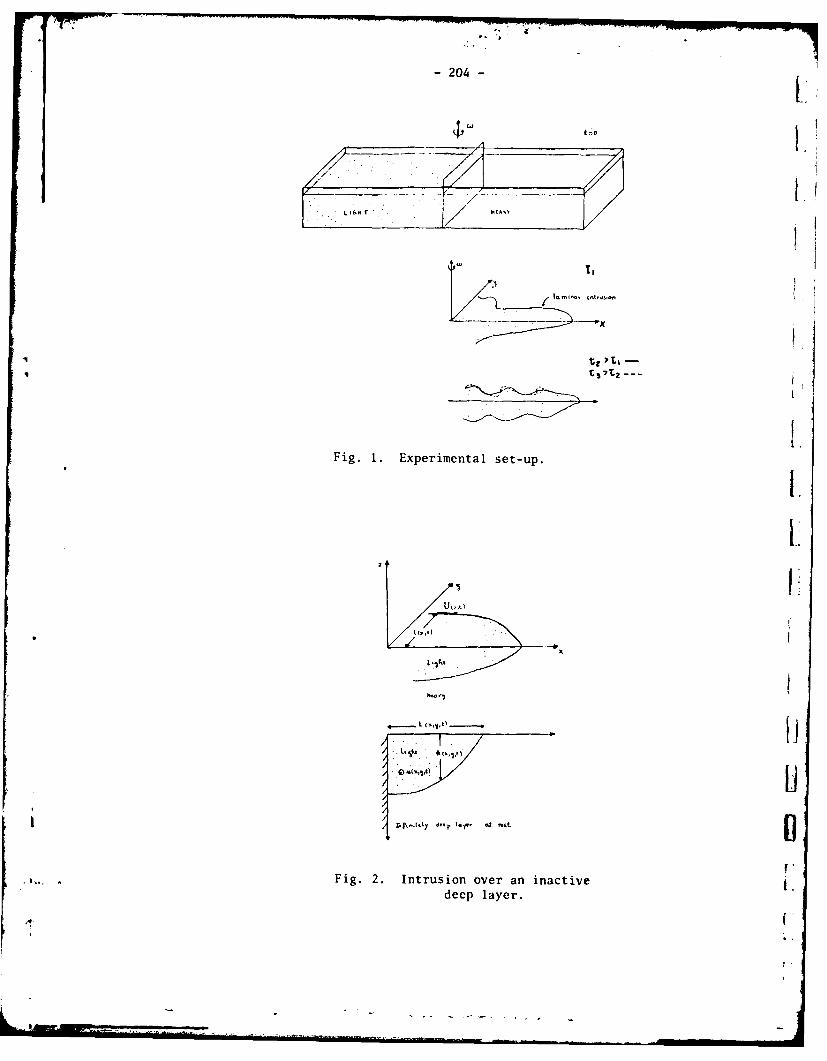
-204- L

L I

I 7t

......,tntvj c

t. o-

--

Fig. i. Experimental set-up.

1.

t.

I:Lt0')

. IiI* '

Fig. 2. Intrusion over an inactive i,

deep layer.

ME

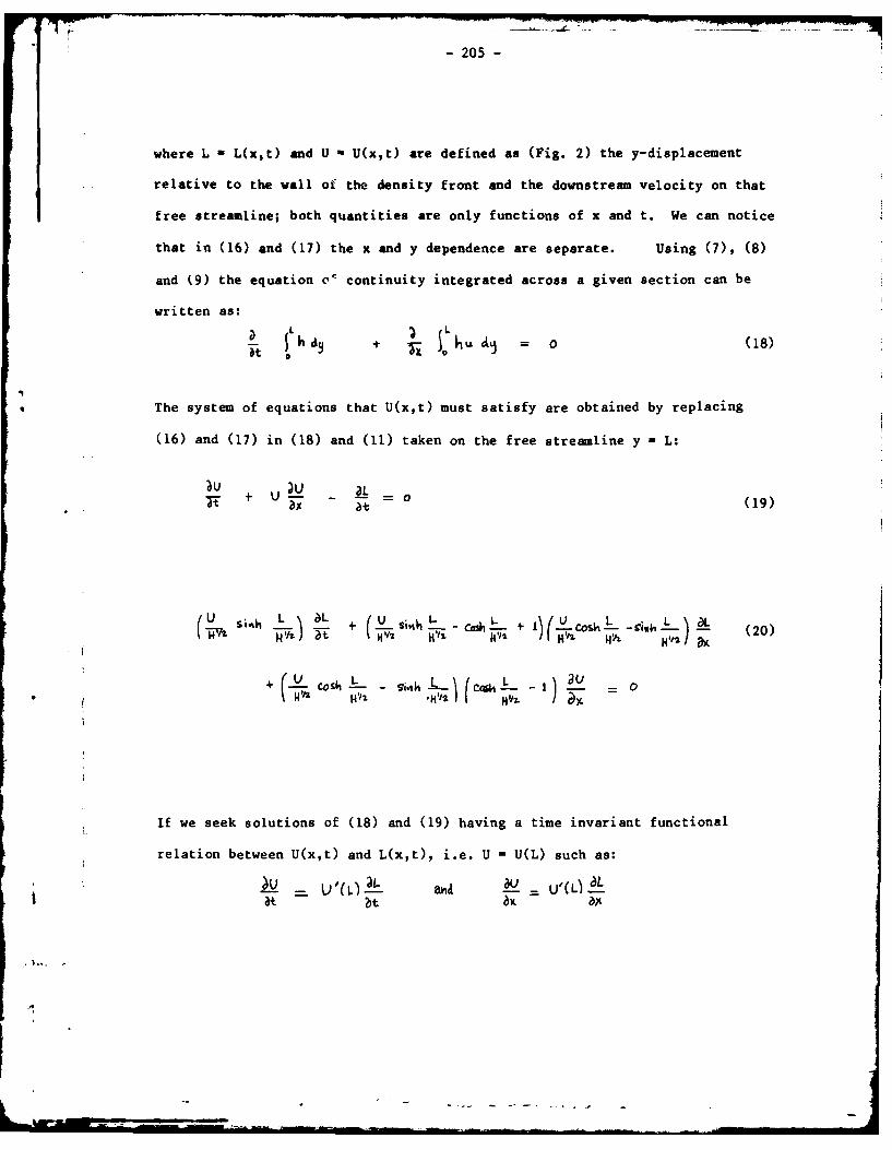
- 205 -

where L L(x,t) and U = U(x,t) are defined as (Fig. 2) the y-displacement

relative to the wall of the density front and the downstream velocity on that

free streamline; both quantities are only functions of x and t. We can notice

that in (16) and (17) the x and y dependence are separate. Using (7), (8)

and (9) the equation o' continuity integrated across a given section can be

written as:

Dt, L = 0 (18)

The system of equations that U(x,t) must satisfy are obtained by replacing

(16) and (17) in (18) and (11) taken on the free streamline y =L:

+ U 079- 21t: (19)

U +(- L. ,---L + -.. 'o., L ) C - .,

If we seek solutions of (18) and (19) having a time invariant functional

relation between U(x,t) and L(x,t), i.e. U = U(L) such as:

Lu L= - ,L

at t b.a

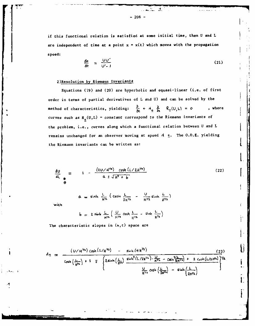
- 206 - 2o

if this functional relation is satisfied at some initial time, then U and L

are independent of time at a point x = x(t) which moves with the propagation

speed:UU"

-- _(21)

U'- I

2)Resolution by Riemann Invariants

Equations (19) and (20) are hyperbolic and equasi-linear (i.e. of first

order in terms of partial derivatives of L and U) and can be solved by the

method of characteristics, yielding: + '4 ± - (U,L) = O , where

curves such as R+(U,L) = constant correspond to the Riemann invariants of

the problem, i.e., curves along which a functional relation between U and L

remains unchanged for an observer moving at speed d t. The O.D.E. yielding

the Riemann invariants can be written as: I

I.du (2U/1I2) Cosh (L/ZM-ft) (22)LU 0= + .

0. SIl cot, Ljz b!ivk

HY2. 2H'/ z

The characteristic slopes in (x,t) space are

Ii

'4/y )

Cs (-1 b~ ~ ) (3

![

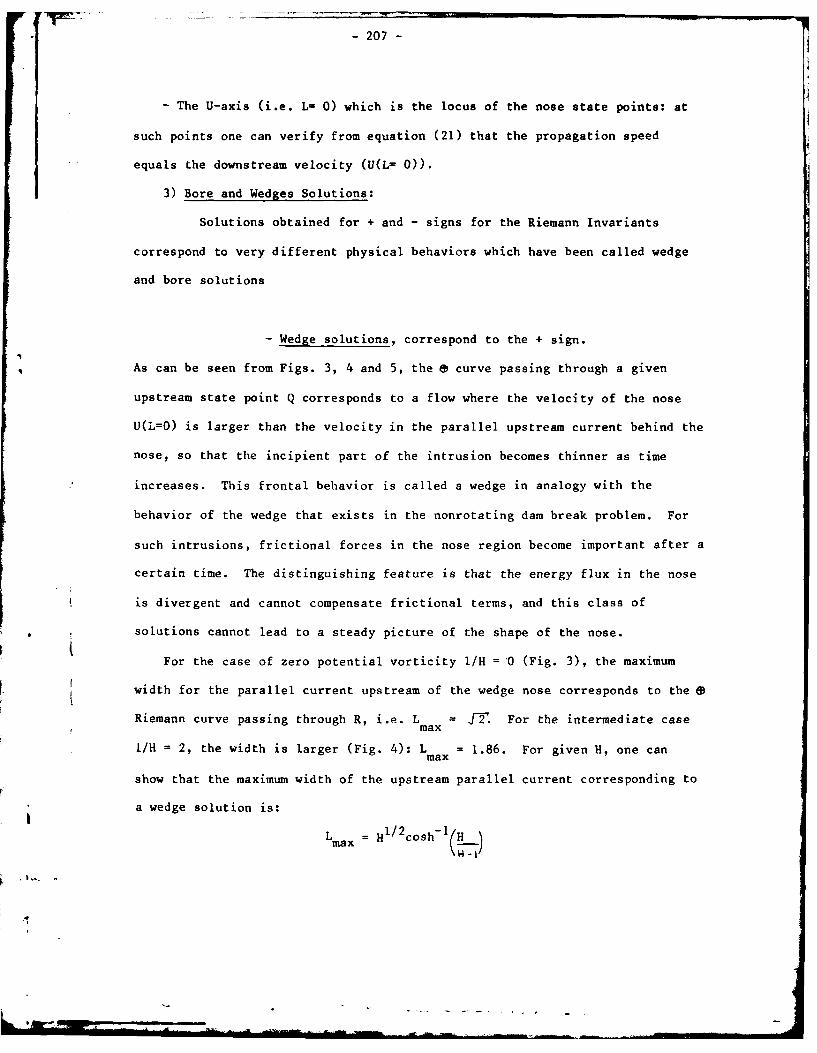
-207-

The U-axis (i.e. L- 0) which is the locus of the nose state points: at

such points one can verify from equation (21) that the propagation speed

equals the downstream velocity (U(L= 0)).

3) Bore and Wedges Solutions:

Solutions obtained for + and - signs for the Riemann Invariants

correspond to very different physical behaviors which have been called wedge

and bore solutions

- Wedge solutions, correspond to the + sign.

As can be seen from Figs. 3, 4 and 5, the & curve passing through a given

upstream state point Q corresponds to a flow where the velocity of the nose

U(L=O) is larger than the velocity in the parallel upstream current behind the

nose, so that the incipient part of the intrusion becomes thinner as time

increases. This frontal behavior is called a wedge in analogy with the

behavior of the wedge that exists in the nonrotating dam break problem. For

such intrusions, frictional forces in the nose region become important after a

certain time. The distinguishing feature is that the energy flux in the nose

is divergent and cannot compensate frictional terms, and this class of

solutions cannot lead to a steady picture of the shape of the nose.

For the case of zero potential vorticity I/H = 0 (Fig. 3), the maximum

width for the parallel current upstream of the wedge nose corresponds to the *

Riemann curve passing through R, i.e. L = J-. For the intermediate case~maxI/H = 2, the width is larger (Fig. 4): L = 1.86. For given H, one can

max

show that the maximum width of the upstream parallel current corresponding to

a wedge solution is:LLma = H1/2 cosh-1 (H

.ma

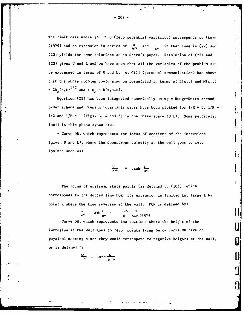
-208-

The limit case where I/H - 0 (zero potential vorticity) corresponds to Stern

(1979) and an expansion in series of U and L in that case in (22) and

(23) yields the same solutions as in Stern's paper. Resolution of (22) and

(23) gives U and L and we have seen that all the variables of the problem can

be expressed in terms of U and L. A. Gill (personal communication) has shown

that the whole problem could also be formulated in terms of L(x,t) and M(x,t)

2h (x,t)1/ 2 where h = h(x,o,t).

Equation (22) has been integrated numerically using a Runge-Kutta second

order scheme and Riemann invariants waves have been plotted for I/H = 09 /H =

1/2 and I/H = I (Figs. 3, 4 and 5) in the phase space (U,L). Some particular

locii in this phase space are:

- Curve OR, which represents the locus of sections of the intrusions

(given U and L), where the downstream velocity at the wall goes to zero

(points such as)

= tanh LHHVI

- The locus of upstream state points (as defined by (10)), which

corresponds to the dotted line PQR: its extension is limited for large L by

point R where the flow reverses at the wall. PQR is defined by:

S - L H C" ( 41411%) L- Curve OH, which represents the sections where the height of the

intrusion at the wall goes to zero: points lying below curve OH have no

physical meaning since they would correspond to negative heights at the wall, Uor is defined by

I f)- __ I . . .. . ilmliml 141/L

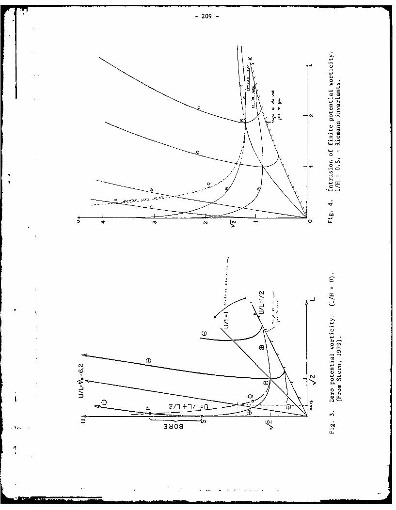
-209-

4 J

.- 4 44 J'-k

4>

4 J CO

- En

0V-

ILII

(N4JN0

0 -n

-j~

N80

- 210 -

For the limit case of 1/H = 1 (Fig. 5), L x o.max

- bore solution: for such solutions the

Riemann e curve passing through a given upstream point P (Figs. 3, 4 and 5)

intersects the U axis at a value U(L = 0) < U(P): that corresponds to the

case of an overrunning bore, where the velocities on the trailing front are

larger than the nose speed so that there is a convergent kinetic energy flux

towards the nose region which will help to compensate frictional effects

there. On the other hand, the overrunning in the nose only occurs until short

wave terms come into being and their dispersion effects will give rise to a

steady shape of the nose that will travel downstream unchanged in shape.

Neither friction nor short waves influences are taken into account in this

approach but the argument that could be evoked here is that there exists an

intermediate region, not too far behind the point where the front strikes the

wall (L = 0), where the short wave solution matches the long wave solution

found in our problem.

For the case of zero potential vorticity (Fig. 3), one can see that no

bore can propagate (i.e., the Riemann 0 curve does not intersect the U-axis)

for upstream states width larger than L = 0.418, for which case the speed of

the nose is zero ("arrested bore").

Figure 4 (I/H = 1/2) (resp. Fig. 5 (1/H = 1) yield L* = 0.422 (resp.

0.426) and for intermediate values of H, numerical integration shows that:

0.418 < L* < 0.426

One can then conclude that the finite value of uniform potential vorticity of

the intrusion seems to play little influence on the limiting width of stable !

bore-like intrusions.

- 211 -

On the other hand, in the band where L < 1, numerical integration shows

also little quantitative differences in the Riemann curves when H varies from

1 to 0 .

For a resolution of an initial-value problem for a given initial repar-

tition, one should notice that the $ and e characteristics have the same

slopes in the region where L = 0, and also that A 4 and A have the same

sign in that region: a numerical resolution using the method of character-

istics should require analytic expansion near the nose L = 0).

4) Quasi-geostrophic Breaking Wave

The comparisons of the topologies of the Riemann curves and other

particular state points locii of Figs. 3, 4 and 5 present an important

similarity. The reader is referred to Stern (1979) for a detailed discussion

(section of "special solutions") of various nonlinear behaviors that can occur

on the trailing geostrophic front. The discussion is mostly based on the

amplitude dispersion of the propagation speed along the Riemann curves. The

similar properties in our cast would be that:

for tL < tanh 1 A and A are positive

for >__ ) tanh L 4 is positive and A is negative

for U tanh L = A_ = 0 (this is important for theH'L1 .H'/ + "Blocking wave" case).

We shall just show here the generalization of a class of special solutions

which is the quasi-geostrophic breaking wave. Let us consider an initial dis-

tribution of a basic state of the front far behind the nose, which would cor-

respond to the largest upstream state (i.e., point R on the upstream state

curve (see for instance, Fig. 4: I/H = 1/2, LR 1.86 and UR = 1.22).

.

P F t' ' ..... . ..... - - -- - --- --- -.- w F.- ---- - wg-

- 212 -

If this upstream state is perturbed in such a way as the perturbed dis- !

tribution corresponds to points lying on the a Riemann curve and lying on

each side of R . UJ(R) = 0 and one can see from equetion (21) that the propa-

gation speed for such a wave has opposite sign for points situated on different

sides of R: for L ) LR (resp. L > LR) , the propagation speed is negative

(resp. positive) and increases in magnitude when L - LR increases in magni-

tude. Therefore, the crest of the front (max L) moves upstream with the

largest speed and the frontal wave pattern steepens on the upstream direc-

tion. The transverse velocity on the free streamline is given by eq. (9)

IL + L U 3L L;

so that v increases as the wave steepens and the current shoots away from the

boundary at the steepest parts of the front. It follows from eq. (16) that

ILE, L

,ra -z ,-6A -l L "

so that the wave is also quasi-geostrophic for the transverse velocity

(V 2 h as well as for the downstream velocity.

ax

IV. Intrusion Overlying a Second Layer of Finite Depth

In this section, the dynamics of the density current intrusion is coupled

with a second layer of uniform depth H2. The intrusion layer is still sup-

posed to have a uniform potential vorticity distribution I/HI . The meaning

of the various notations are given on Fig. 6. The equations in the same non-

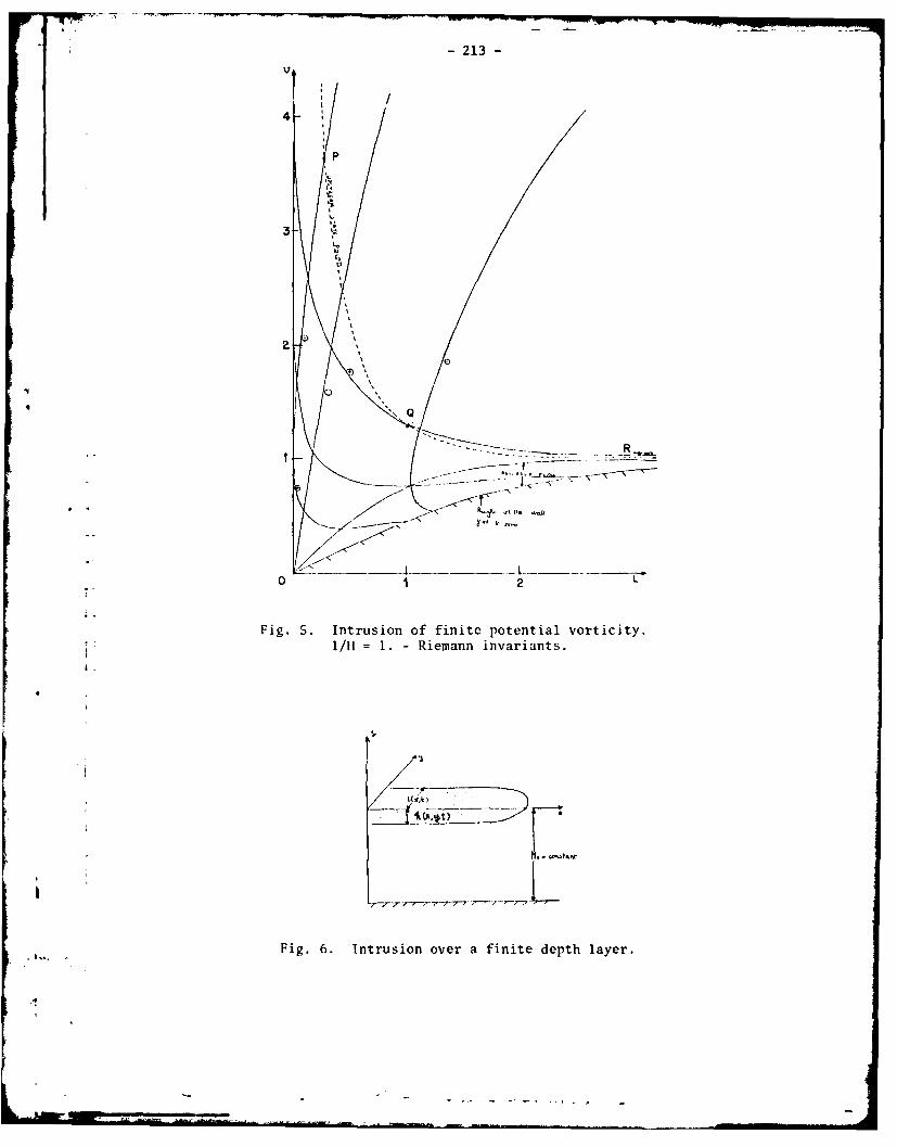
- 213 -

U

4

P

3Q

a2l/ 1-,--- R i a

0 1 2

Fig, 5. Intrusion of finite potential vorticity.[: 1/tt = 1. - Riemann invariants.

i.5

Fig. 6. Intrusion over a finite depth layer.

.4

-214-

dimensional quantities as in Section III, are:I.

1st layer

x-momentum equation: (24)

Ul - (I- 1A 1)vY +hs u.x + 'A-A

vorticity equation: (25)

I - IL

continuity equation: (26)

ht (6)X + . ) 0

2nd layer

Margules relation: (27)

LLI - zL= -

vorticity equation (28)

LL24 = t /H1 1.Equations (26), (27) and (28) yield:

- k- 1 =(29)

where we have introduced the "equivalent depth" H:

H .L 4 .-t2L Iot..k , + 14z=II (30)4 , t H L 4 , -I

Equation (29) has the same form as (15) found in section III, but with an

equivalent depth in the 2-layer case. In addition to the boundary conditions Lgiven in section III, we need an extra boundary condition for the downstream 1velocity in the second layer v2(xy,t). Outside the region lying under the

4,.

4 ii

- 215 -

vertical of the density current intrusion, h(x,yt) = 0 and equation (28)

yields u =0 since there can be no motion u in the second layer that

can extend to y -, - , this implies u2 (x,yt) - 0, outside the vertical of

the intrusion rgion, so that the matching condition at the vertical of the

free streamline is

L, ( .{, L t), = o (31)

Solutions of (26), (27) and (28) for ui(x,y,t), u2 (x,y,t) and h(x,y,t),

satisfying the boundary conditions (31) and (8) are:

S(32)

LLU,j,-+.) = .1. ( u + - L) + H. si" + UCosk (33)

S L)+.U(I - (3

14 H'I

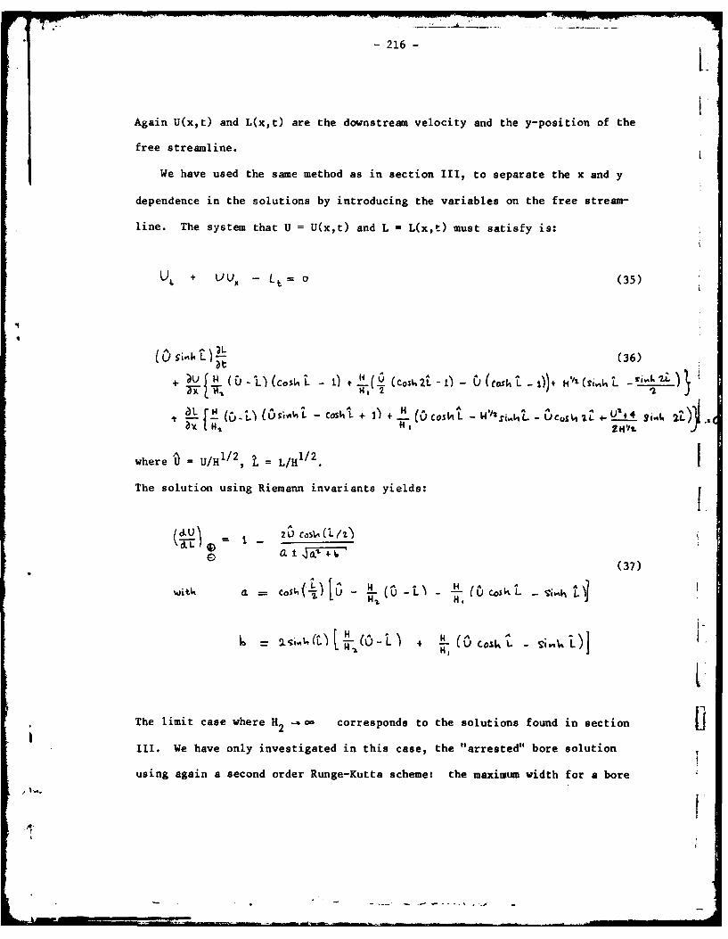
-216-

Again U(x,t) and L(x,t) are the downstream velocity and the y-position of the

free streamline.

We have used the same method as in section III, to separate the x and y

dependence in the solutions by introducing the variables on the free stream-

line. The system that U = U(x,t) and L = L(x,t) must satisfy is:

Ut + X - L= o (35)

+e s Lu i (o nL) (Cu isRi t i elds. (I.Li rr. . )

h4 2T

where U = UIHlI, L/Hl/2

The solution using Riemann invariants yields:

(37)

uj% a =cosLij UL - UL( i ~ C csk L - Vii-4

= . ¢j- (Af + 4( c~

L

The limit case where H2 --0o corresponds to the solutions found in sectionI

1II. We have only investigated in this case, the "arrested" bore solution

using again a second order Runge-Kutta scheme: the maximum width for a boreA r

-217-

to propagate for H1 = H 2= 1 is

=* 0.4185

so that the inclusion of the dynamics of a second layer seems to play little

influence on the numerical result found in section Ill.

V. Conclusion

The results of the previous sections concerning the maximum width of a

bore-type intrusion strongly lead to the conjecture that there exists a limit-

ing width of the boundary current far upstream of the nose, in the region where

the current appears to be both laminar and steady. The existence of this maxi-

mum width is a consequence of the analytical resolution of the dynamics of the

flow, whereas previous studies have evoked dimensional arguments to limit this

width. Therefore, the need is felt for a careful experimental measurement of

this width, using immiscible fluids (such as silicon oil and a mixture of

ethyl and water in order to obtain small density differences) so that the

interface between the two fluids is sharply defined and that no mixing

occurs. If the actually measured maximum width exceeds the theoretical value

found here, this will stimulate further theoretical investigations to relax

the long-wave assumption in the downstream direction, and include short waves

dispersion effects at the nose of the intrusion, which could lead to a steady

shape of the nose like those observed in the preliminary experiments.

In this work, an outline of some non-linear interaction on the trailing

front has been sketched. A thorough study would require a numerical resolution

of given initial-value repartitions. It would be interesting to test, par-

ticularly if one can reproduce numerically instabilities such as those observed

in the experiment. However, the theory is strongly restricted by the assump-

tion of uniform potential vorticity distribution in each layer, since this

filters out all the geostrophical unstable modes for which (Stern, 1975, page

-218 -

68-71) a necessary condition for amplifying waves in that the gradient of the

basic potential vorticity must assume both positive and negative values within Lthe cross-stream interval of the jet.

The mathematical method used in the two-layer case may be used for an Lanalytical approach of the classical frontal waves problem as initially posed

by the Norwegian school (Orlanski, 1968) for an atmospheric front intersecting

the ground.

Acknowledgements

I would like to thank Melvin Stern for a very stimulating and enjoyable

summer's work. I am also grateful to George Veronis, who suggested to me the

initial subject of this work, and to Adrian Gill for his helpful coments.

REFERENCES

Barr, D.I.H., 1967. Densimetric exchange flow in rectangular channels. III.

Large scale experiments. La Houille Blanch, 22, 619-32.

Gill, A., 1976. Adjustment under gravity in a rotating channel flow. Jour.

Fluid Mech., 77,, pt. 3, 603-631.

Gill, A. and E. Schumann, 1979. Topographically induced changes in the

structure of an inertial coastal jet: application to the Agulhas Current.

Submitted to D.S.R.

Orlanski, I., 1968. Instability of frontal waves. Jour. Atmos. Sci., 25,

n02, 178-200.

Stern, M., 1975. Ocean circulation physics, Academic Press, New York.

Stern, M., 1979. Geostrophic fronts, bores, breaking and blocking waves.

Submitted to

Wadhams, P., A. E. Gill and P. F. Linden, 1979. Transects by submarine of the

East Greenland Polar Front. Submitted to D.S.R.

Whitehead, J. A., A. Leetma and R. A. Knox, 1974. Rotating hydraulics of

strait and sill flows. Jour. Geophys. Fluid Dyn., 6, 101-105.

t

.4

Documents

455 WOODS HOLE OCEANOGRAPHIC INSTITUTION MASS · PDF fileAD-AGG82 455 WOODS HOLE OCEANOGRAPHIC INSTITUTION MASS FIG8/ ... Charles D. Hollister ... Bert University of Gothenburg