arX

iv:1

506.

0377

6v2

[qu

ant-

ph]

22

Oct

201

5

Witnessing causal nonseparability

Mateus Araújo,1, 2 Cyril Branciard,3 Fabio Costa,1, 2, 4 Adrien Feix,1, 2 Christina Giarmatzi,4, 5 and Caslav Brukner1, 2

1Faculty of Physics, University of Vienna, Boltzmanngasse 5 1090 Vienna, Austria2Institute for Quantum Optics and Quantum Information (IQOQI), Boltzmanngasse 3 1090 Vienna, Austria

3Institut Néel, CNRS and Université Grenoble Alpes, 38042 Grenoble Cedex 9, France4Centre for Engineered Quantum Systems, School of Mathematics and Physics,

The University of Queensland, St Lucia, QLD 4072, Australia5Centre for Quantum Computer and Communication Technology,

School of Mathematics and Physics, University of Queensland, Brisbane, QLD 4072, Australia(Dated: October 23, 2015)

Our common understanding of the physical world deeply relies on the notion that events areordered with respect to some time parameter, with past events serving as causes for future ones.Nonetheless, it was recently found that it is possible to formulate quantum mechanics withoutany reference to a global time or causal structure. The resulting framework includes new kinds ofquantum resources that allow performing tasks – in particular, the violation of causal inequalities –which are impossible for events ordered according to a global causal order. However, no physicalimplementation of such resources is known. Here we show that a recently demonstrated resourcefor quantum computation – the quantum switch – is a genuine example of “indefinite causal order”.We do this by introducing a new tool – the causal witness – which can detect the causal nonseparabilityof any quantum resource that is incompatible with a definite causal order. We show however thatthe quantum switch does not violate any causal inequality.

I. INTRODUCTION

It is commonly assumed that information is pro-cessed through a series of operations which are per-formed according to a specific order. This is justifiedby the assumption of a global, underlying time pa-rameter according to which all operations can be or-dered. A convenient representation of this structureis that of a circuit [1], Fig. 1(a), in which systems are“wires” that connect “boxes”, which represent opera-tions performed on the systems. At a more abstractlevel, a circuit only imposes a given causal structurebetween operations, as the time order between oper-ations that can be performed in parallel is irrelevant.The circuit framework is also ubiquitous in the studyof quantum foundations to formalize generalized, pos-sibly post-quantum, probabilistic theories [2–5].

It has been suggested that such a framework mightbe too restrictive to encompass the most generalkinds of information processing allowed by quantumphysics [6]. For example, one can consider protocolsin which the order between different operations is con-trolled by a quantum degree of freedom. It has beenshown that such protocols exploiting a so-called “quan-tum switch” not only provide computational advan-tage over standard, time-ordered, ones [7, 8], but theyare also physically realizable and a first experimentalproof-of-principle has been recently demonstrated [9].At a more fundamental level, an underlying time orcausal order might not be well-defined in a theory thatcombines the dynamical causal structure of general rel-ativity and the probabilistic nature of quantum mechan-

ics [10–12].It is therefore natural to ask what the most general re-

sources allowed by quantum mechanics beyond the cir-cuit model are. In Ref. [13] the process matrix formalismwas proposed as a general framework to describe re-sources that can be accessed in “local laboratories” andwhich are locally in agreement with quantum physics,Fig. 1(b).

Causal relations are defined operationally in this for-malism. If, for example, through appropriate statepreparations, an agent A can influence the outcomesof measurements performed by an agent B, whereas Bis never able to influence A, then A causally precedesB by definition and, in this case, the physical resourcesavailable to them can in fact be represented as a circuit.A first example of a resource that cannot be representedas a circuit is a probabilistic mixture of circuits: a defi-nite order still exists between A and B in each run ofan experiment, but which order is realized in a givenrun is only specified according to some probability dis-tribution. Resources compatible with a definite causalorder, in this broader sense, are called causally separa-ble. Surprisingly, the formalism also allows for causallynonseparable resources, which are incompatible with anydefinite order between operations. It was found thata set of agents with access to a specific causally non-separable resource could perform a task, the violationof a causal inequality, which is impossible for arbitrarycausally ordered strategies, even allowing probabilisticmixtures of orders [13]. However, there is no physicalinterpretation for such resources and no physically re-alizable protocol is known which can violate a causalinequality.

2

M1

M2

M3

M4

(a)

M1

M2M3

M4

(b)

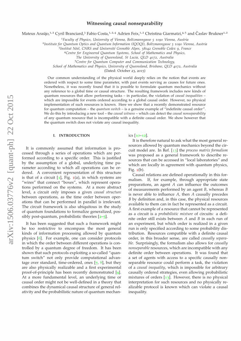
Figure 1. (a) If the operations Mi of local agents are per-formed in a definite causal sequence, they can be representedas gates in a circuit, where information flows from bottom totop. (b) A process matrix formalizes a resource in which theorder between operations may not be fixed. A probabilisticmixture of different orders is an example of a process ma-trix that does not correspond to a circuit. Still, in this caseoperations are performed in a well-defined order in each ex-perimental run; the most general resource with this propertyis called causally separable. The process matrix formalism alsoallows for the more general case of causally nonseparable re-sources [13].

It is therefore not completely clear what is the pre-cise relation between “quantum correlations with nocausal order”, which violate causal inequalities, andphysically implementable resources, such as the quan-tum switch, which outperform causally ordered ones.To understand this relation, a crucial observation is thatthe causal inequalities are device-independent constraints:they are formulated independently of the physics of thesystems or the specific apparatuses employed. On theother hand, the tasks discussed in Refs. [7, 8] includeadditional assumptions, as for example that in each lab-oratory quantum systems of a definite dimension haveto be used. It is clear that, given additional restrictions,it is more difficult for causally-ordered agents to per-form certain tasks and, consequently, it can be easier todetect the lack of causal order in a physical resource.

The aim of the present work is to develop a generalframework for the device-dependent detection of causalnonseparability. The central tool we introduce is whatwe call a causal witness, which represents a set of quan-tum operations, such as unitaries, channels, state prepa-rations, and measurements, whose expectation valueis non-negative as long as all the operations are per-formed in a definite causal order, i.e., as long as onlycausally separable resources are used. The observationof a negative expectation value is thus sufficient to con-clude that the operations were not performed in a def-inite order. The concept is analogous to that of entan-

glement witness: an observable that has a non-negativeexpectation value for separable states but can have anegative expectation value for specific entangled states.

We find that, for every causally nonseparable process,it is possible to construct a causal witness that detectsit. Importantly, and differently from the case of entan-glement witnesses, it is possible to use this method towrite necessary and sufficient conditions for causal sep-arability in a form that can be checked efficiently usingsemidefinite programming (SDP).

The tools developed are applied to the study of thequantum switch as a resource within the process ma-trix formalism. We show that, indeed, the quantumswitch corresponds to a causally nonseparable process.We show that the protocol of Ref. [7] can be reformu-lated as a causal witness which detects the causal non-separability of the quantum switch. We also find new,more efficient witnesses, which could be useful for ex-perimental implementations.

We finally address the question of whether the quan-tum switch can pass any device-independent test ofcausal nonseparability. As it turns out, this is not possi-ble: we prove that a broad class of resources, includingthe quantum switch, cannot violate any causal inequal-ity.

The paper is organized as follows: In Section II, wereview the process matrix formalism, giving a conve-nient characterization of general and causally separa-ble process matrices for the cases of interest. In Sec-tion III, we introduce and characterize the central con-cept of causal witness, and we present efficient algo-rithms for finding witnesses and for proving the causal(non)separability of a general process matrix. In Sec-tion IV we formalise the quantum switch as a processmatrix. We proceed to prove its causal nonseparabilityin Section V, through the use of causal witnesses. Onesuch witness is the task proposed in Ref. [7], that we op-timize to increase its resistance to noise. Finally, we clar-ify in Section VI the link between causal witnesses andcausal inequalities and show that the quantum switchcannot violate any causal inequality.

II. THE PROCESS MATRIX FORMALISM

In the general scenario we consider in this paper, Nparties Ai establish correlations by exchanging physicalsystems between their laboratories. Each party openstheir laboratory only once to let an incoming systementer and to send an outgoing system out; they canact on these systems by performing an arbitrary opera-tion in their local laboratory, which can yield differentmeasurement outcomes. The causal relations betweenthe parties (i.e., the ordering of events) are not a priorispecified. The most general situation compatible with

3

the assumption that the operations performed in each lo-cal laboratory can be described by the quantum formalismcan be conveniently represented in the “process ma-trix” formalism introduced in Ref. [13]. This extends the“comb” formalism of Ref. [14], which describes causallyordered quantum networks. The aim of the formalismis to characterize all possible probability distributionsthat can be obtained in our general scenario. The keyconcept is that of a process, which can be understood asthe external resource determining the statistics of the lo-cal operations, and which generalizes both the notionsof quantum state and of quantum channel. The processmatrix is a useful mathematical representation of such aconcept. We shall use these two terms interchangeably.

A. Local operations

Each party A acts in a local quantum laboratory, whichcan be identified by an input Hilbert space HAI andan output Hilbert space HAO . The dimensions dAI

anddAO

of input and output spaces do not have to be equal,as ancillary systems can be added or discarded duringan operation; we shall nevertheless assume throughoutthe paper that all Hilbert spaces are finite-dimensional.According to quantum theory, the most general localoperation is described by a completely positive (CP),trace non-increasing map MA : AI → AO [15], wherewe write AI , respectively AO, for the space of hermi-tian linear operators over the Hilbert space HAI , resp.HAO . Examples of CP maps are deterministic opera-tions, such as unitaries or quantum channels, or (gen-eralized) measurements. In general, a label a, denot-ing the measurement outcome, is associated with theCP map MA

a . The choice of operation (e.g. of mea-surement setting) is represented by an instrument [16],which is defined as the collection J A =

MAa

m

a=1of CP maps associated to all measurement outcomes,characterized by the property that ∑

ma=1 MA

a is CP andtrace-preserving (CPTP). An instrument generalizes thenotion of POVM (positive operator-valued measure) toinclude the transformations applied to the system; itreduces to a POVM for 1-dimensional output spaces.When the choice of operation is described by a classicalvariable x, we will express such a dependence explicitly

as J Ax =

MA

a|xm

a=1.

A convenient representation of CP maps is given bythe Choi-Jamiołkowski (CJ) isomorphism [17]. For a CPmap MA

a : AI → AO, its corresponding CJ matrix isdefined here as

MAI AOa :=

[I ⊗MA

a (|1〉〉〈〈1|)]T

∈ AI ⊗ AO, (1)

where I is the identity map, |1〉〉 ≡ |1〉〉AI AI :=

∑j|j〉AI ⊗ |j〉AI ∈ HAI ⊗ HAI is a (non-normalized)

maximally entangled state, and T denotes matrix trans-position with respect to the chosen orthonormal basis|j〉AI of HAI . Some useful properties of the CJ iso-morphism are given in Appendix A 1. A map is com-pletely positive if and only if its CJ representation ispositive semidefinite, while the trace-preserving condi-tion is equivalent to trAO

MAI AO = 1AI (where trAO

de-notes the partial trace over AO, and 1

AI is the identitymatrix in AI). An instrument is therefore equivalentlyrepresented as a set

M

AI AOa

m

a=1, M

AI AOa ≥ 0, trAO

m

∑a=1

MAI AOa = 1

AI .

(2)

B. Process matrices

As discussed in Ref. [13], requiring that quantum me-chanics holds locally implies that the probability thatthe N parties Ai observe the outcomes a1, . . . , aN , for achoice of operations x1, . . . , xN , is a multilinear function

P(MA1

a1|x1, . . . ,MAN

aN|xN

)of the corresponding CP maps

MA1

a1|x1, . . . ,MAN

aN|xN. Using the CJ representation, it was

shown that these probabilities can then be expressed as

P(

MA1

a1|x1, . . . , MAN

aN |xN

)

= tr[(

MA1

I A1O

a1|x1⊗ . . . ⊗ M

ANI AN

O

aN |xN

)W

], (3)

for some hermitian operator W ∈ A1I ⊗ A1

O ⊗ . . .⊗ ANI ⊗

ANO called a process matrix, which describes the general

quantum resource connecting the local laboratories.The set of valid process matrices is defined by requir-

ing that probabilities are well-defined – that is, theymust be non-negative and must sum up to 1 – for allpossible operations, including operations that involve,in each laboratory, local interactions with ancillary sys-tems that may be entangled with the other laboratories.As we show in Appendix B, these conditions are equiv-alent to

W ≥ 0, (4)

tr W = dO, (5)

W = LV(W), (6)

where dO = dA1O

. . . dANO

, and LV is a projector onto the

linear subspace LV ⊂ A1I ⊗ A1

O ⊗ . . . ⊗ ANI ⊗ AN

O de-fined in Appendix B. We will denote the closed convexcone of non-normalized processes defined by (4) and (6)by W .

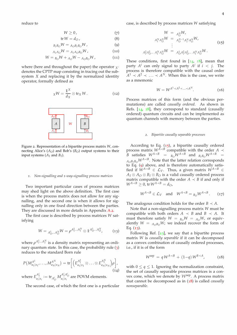
In the case of two parties A (Alice) and B (Bob), seeFigure 2, these conditions on W ∈ AI ⊗ AO ⊗ BI ⊗ BO

4

reduce to

W ≥ 0 , (7)

tr W = dO , (8)

BI BOW = AOBI BO

W , (9)

AI AOW = AI AOBO

W , (10)

W = BOW + AO

W − AOBOW , (11)

where (here and throughout the paper) the operator X·denotes the CPTP map consisting in tracing out the sub-system X and replacing it by the normalized identityoperator, formally defined as

XW =1

X

dX⊗ trX W . (12)

A W B

AO

AI

BO

BI

Figure 2. Representation of a bipartite process matrix W, con-necting Alice’s (AO) and Bob’s (BO) output systems to theirinput systems (AI and BI ).

1. Non-signalling and 1-way-signalling process matrices

Two important particular cases of process matricesmay shed light on the above definition. The first caseis when the process matrix does not allow for any sig-nalling, and the second one is when it allows for sig-nalling only in one fixed direction between the parties.They are discussed in more details in Appendix A 2.

The first case is described by process matrices W sat-isfying

W = A1O...AN

OW = ρA1

I ...ANI ⊗ 1

A1O...AN

O , (13)

where ρA1I ...AN

I is a density matrix representing an ordi-nary quantum state. In this case, the probability rule (3)reduces to the standard Born rule

P(

MA1

a1|x1, . . . , MAN

aN|xN

)= tr

[(E

A1I

a1|x1⊗ . . . ⊗ E

ANI

aN |xN

)ρ

],

(14)

where EAi

I

ai|xi:= trAi

OM

AiI Ai

O

ai|xiare POVM elements.

The second case, of which the first one is a particular

case, is described by process matrices W satisfying

W = ANO

W,

ANI AN

OW =

AN−1O AN

I ANO

W,...

A2I A2

O... ANI AN

OW = A1

O A2I A2

O... ANI AN

OW .

(15)

These conditions, first found in [14, 18], mean thatparty Ai can only signal to party Aj if i < j. Theprocess is therefore compatible with the causal orderA1 ≺ A2 ≺ . . . ≺ AN . When this is the case, we writeas a mnemonic

W = WA1≺A2≺ ...≺AN. (16)

Process matrices of this form (and the obvious per-mutations) are called causally ordered. As shown inRefs. [14, 18], they correspond to standard (causallyordered) quantum circuits and can be implemented asquantum channels with memory between the parties.

2. Bipartite causally separable processes

According to Eq. (15), a bipartite causally orderedprocess matrix WA≺B compatible with the order A ≺B satisfies WA≺B = BO

WA≺B and BI BOWA≺B =

AOBI BOWA≺B. Note that the latter relation corresponds

to Eq. (9) above, and is therefore automatically satis-fied if WA≺B ∈ LV . Thus, a given matrix WA≺B ∈AI ⊗ AO ⊗ BI ⊗ BO is a valid causally ordered processmatrix compatible with the order A ≺ B if and only ifWA≺B ≥ 0, tr WA≺B = dO,

WA≺B ∈ LV and WA≺B = BOWA≺B . (17)

The analogous condition holds for the order B ≺ A.Note that a non-signalling process matrix W must be

compatible with both orders A ≺ B and B ≺ A. Itmust therefore satisfy W = BO

W = AOW, or equiv-

alently W = AOBOW; we indeed recover the form of

Eq. (13).Following Ref. [13], we say that a bipartite process

matrix W is causally separable if it can be decomposedas a convex combination of causally ordered processes,i.e., if it is of the form

Wsep = q WA≺B + (1−q)WB≺A, (18)

with 0 ≤ q ≤ 1. Ignoring the normalization constraint,the set of causally separable process matrices is a con-vex cone, which we denote by Wsep. A process matrixthat cannot be decomposed as in (18) is called causallynonseparable.

5

3. Tripartite causally separable processes

In this paper we will define tripartite causal sepa-rability only for processes where the output space ofthe third party C (Charlie) is trivial, i.e., dCO

= 1 (seeFigure 3). As C cannot signal to the other parties, ev-ery process of this kind if compatible with C being last.Thus, only two causal orders are relevant in this case:A ≺ B ≺ C and B ≺ A ≺ C. The conditions for pro-cess matrices being compatible with these orders are,according to equation (15),

WA≺B≺C = COWA≺B≺C, (19)

CI COWA≺B≺C = BOCI CO

WA≺B≺C, (20)

BI BOCI COWA≺B≺C = AOBI BOCI CO

WA≺B≺C, (21)

and

WB≺A≺C = COWB≺A≺C, (22)

CI COWB≺A≺C = AOCI CO

WB≺A≺C, (23)

AI AOCI COWB≺A≺C = BO AI AOCI CO

WB≺A≺C. (24)

Since these three conditions together define a linearsubspace, we can write them more succinctly as

WA≺B≺C = LA≺B≺C(WA≺B≺C), (25)

WB≺A≺C = LB≺A≺C(WB≺A≺C), (26)

where LA≺B≺C and LB≺A≺C are the projectors onto theaforementioned subspaces.

A W B

C

AO

AI

BO

BI

CI

Figure 3. Representation of a tripartite process matrix Wwhere one party has trivial output dCO

= 1. It can be seenas connecting Alice’s (AO) and Bob’s (BO) output systems toAlice, Bob and Charlie’s input systems AI , BI and CI .

Therefore, when C’s output space is trivial, we willcall a tripartite process matrix Wsep causally separableif it is of the form

Wsep = q WA≺B≺C + (1−q)WB≺A≺C, (27)

with 0 ≤ q ≤ 1. Ignoring the normalization constraint,this defines a convex cone Wsep

3C . We will use this def-inition in Section V to show that a recently introduced

tripartite quantum resource, which yields information-processing advantages with respect to causally orderedprocesses [7, 8], is causally nonseparable.

The generalization of the notion of causal separabilityto a larger number of parties, with arbitrary dimensionsof the output spaces, is not trivial. The reason is thatone can consider situations in which an agent, throughher local operations, could modify a classical variablethat determines the causal order of agents in her future.In such a “classical switch”, operations would still becausally ordered in each run of an experiment, but itwouldn’t be possible to write the corresponding processmatrix as a mixture of causally ordered ones. As thisissue does not affect the cases treated here, we shall notconsider it further. A more detailed analysis will bepresented in an upcoming work [19].

III. CAUSAL WITNESSES

A. Definition and characterization

In this section we develop mathematical tools to iden-tify, in the bipartite case, which process matrices arecausally separable and which are not. In analogy withentanglement witnesses [20], we call a hermitian oper-ator S a causal witness (or witness, simply) if1

tr[S Wsep] ≥ 0 (28)

for every causally separable process matrix Wsep. Thisdefinition is motivated by the separating hyperplanetheorem [21]: since the set of causally separable pro-cesses is closed and convex, for every causally nonsep-arable process matrix Wns there exists a causal witnessSWns such that tr[SWnsWns] < 0.

To construct a witness for a given nonseparable pro-cess, we will start by characterizing the set of all causalwitnesses in terms of linear constraints on a convexcone. This will allow us to cast the problem of find-ing a witness as an SDP problem. First, note that (28) isequivalent to

tr[S WA≺B] ≥ 0 ∀WA≺B , (29a)

tr[S WB≺A] ≥ 0 ∀WB≺A . (29b)

Let us focus on condition (29a). Using Eq. (17) and not-ing that for any valid process matrix W, BO

W is a validcausally ordered process matrix compatible with the or-der A ≺ B, one finds that (29a) is equivalent to

tr[S(BO

W)] ≥ 0 ∀W ∈ LV , W ≥ 0 . (30)

1 Note that the bound 0 and the sign of the inequality are arbitrary;we choose them as in Eq. (28) for mathematical convenience.

6

Thinking of the trace as the Hilbert-Schmidt inner prod-uct and noting that the map BO

· is self-dual, we havethat

tr[S(BO

W)]= tr

[(BO

S)W], (31)

and it is sufficient that BOS ≥ 0 for the right-hand-sideto be non-negative for all valid W. An analogous argu-ment shows that AO

S ≥ 0 is sufficient to satisfy condi-tion (29b). We conclude that for S to be a causal witness,it is sufficient that

BOS ≥ 0 and AO

S ≥ 0. (32)

Note also that adding an operator S⊥ belonging tothe orthogonal complement L⊥

V of LV to any witnessS gives another valid witness, since tr[(S + S⊥)W] =tr[SW] for any valid process matrix W. It turns out thatthis suffices to completely characterize the set of causalwitnesses, as stated in the following theorem:

Theorem 1. A hermitian operator S ∈ AI ⊗ AO ⊗ BI ⊗ BO

is a causal witness if and only if S can be written as

S = SP + S⊥, (33)

where SP and S⊥ are hermitian operators such that

BOSP ≥ 0, AO

SP ≥ 0, LV(S⊥) = 0 . (34)

The rather technical proof of this theorem is relegatedto Appendix C. This theorem provides a characteriza-tion of the closed convex cone of causal witnesses S .

Since S⊥ does not change the expectation valuetr[SW], it can freely be chosen to be for instance

S⊥ = LV(SP)− SP, (35)

so that S = LV(SP). This has the effect of restrictingwitnesses to the subspace of valid processes LV , whichhave the following characterization:

Corollary 2. A hermitian operator S ∈ LV is a causal wit-ness if and only if there exists a hermitian operator SP ∈AI ⊗ AO ⊗ BI ⊗ BO such that S = LV(SP), BO

SP ≥ 0, and

AOSP ≥ 0.

This restricted set of causal witnesses is also a closedconvex cone, which we denote by SV = S ∩ LV .

One could define witnesses as belonging to SV in-stead of S , since both sets are as powerful in detectingcausal nonseparability. However, some physically moti-vated witnesses, such as those presented in Section V B(for the tripartite case), do not belong to SV , which iswhy we use the more general definition that witnessesbelong to S .

B. Finding causal witnesses

The previous characterization of the convex cone ofcausal witnesses allows one to efficiently check thecausal nonseparability of any process matrix W throughalgorithms for semidefinite programming (SDP) [22].They output a causal witness if W is causally non-separable, and an explicit decomposition in terms ofcausally ordered process matrices otherwise.

The idea is simply to minimize tr[S W] over the coneof causal witnesses2 SV , and check whether we obtaina negative value or not. Note that in order to maketr[S W] lower bounded (to avoid getting a value −∞

for causally nonseparable process matrices) a normali-sation constraint on the witnesses has to be imposed.This normalisation is arbitrary – any constraint thatmakes SV compact suffices – and different normalisa-tion choices give rise to different interpretations for thevalue of tr[S W]. We shall normalise the witnesses byimposing that tr[S Ω] ≤ 1 for every (normalised) pro-cess matrix Ω, for − tr[S W] can then be interpreted as ameasure of causal nonseparability, as we shall see laterin this subsection. In order to be able to use it in theSDP problem we still need to write this normalisationas a conic constraint. To do so, we extend the constrainttr[S Ω] ≤ 1 to non-normalised process matrices by lin-earity:

tr[S Ω] ≤ tr[Ω]/dO, (36)

which is equivalent to

tr[(1/dO − S)Ω] ≥ 0 (37)

for all Ω ∈ W . Recalling that S is assumed to be inSV ⊂ LV , this means that 1/dO − S ∈ W∗

V := W∗ ∩LV ,where W∗ is the dual cone of W – that is, the cone ofhermitian operators that have non-negative trace withprocess matrices.

To test the causal nonseparability of a given processmatrix W, we are thus led to define the following SDPproblem:

min tr[SW]

s.t. S ∈ SV , 1/dO − S ∈ W∗V ,

(38)

which is written explicitly in terms of positive semidef-inite constraints in Appendix D.

If the solution of the SDP problem (38) leads to a neg-ative expectation value of S, one can conclude that Wis causally nonseparable, since SDP algorithms can be

2 In principle minimizing over S instead of SV would lead to thesame value for tr[S W], but this causes technical problems as ex-plained in Appendix E.

7

guaranteed3 to find the optimal solution [22]. In sucha case, the optimal solution S∗ provides an explicit wit-ness to verify the causal nonseparability of W. On theother hand, if tr[S∗ W] = 0, one concludes that W iscausally separable, and an explicit decomposition ofW into causally ordered processes is given by the SDPproblem dual to (38) (this can be seen explicitly fromthe representation of the SDP problem (39) given in Ap-pendix D). As shown in Appendix E, this dual is

min tr[Ω]/dO

s.t. W + Ω ∈ Wsep, Ω ∈ W ,(39)

where Wsep is the cone of non-normalized causally sep-arable process matrices, as previously defined. Further-more, the optimal value tr[Ω∗]/dO of problem (39) isrelated to the optimal value tr[S∗W] of problem (38)through

tr[Ω∗]/dO = − tr[S∗W]. (40)

This gives an operational meaning to − tr[S∗W]. Asshown in Appendix E, this quantity corresponds to theminimal λ ≥ 0 such that

11 + λ

(W + λ Ω

)(41)

is causally separable, optimized over all valid, nor-malised processes Ω. In other words, it quantifies theresistance of W to the worst-case noise. This is ananalogue of the measure of entanglement called gener-alised robustness, which quantifies the resistance of theentanglement of a quantum state to worst-case noise[23]. It turns out that for our case the interpretationof − tr[S∗W] as a measure of causal nonseparability is alsotenable, as it respects some simple axioms that we pro-pose in Appendix F. For this reason, we define the gen-eralised robustness of a process W as

Rg(W) = − tr(S∗W). (42)

Again in analogy with the case of entanglement mea-sures, one can also define the random robustness [24] ofW as is its resistance to “white noise”, which can be de-fined as the process that sends maximally mixed statesto each laboratory, independently of the local opera-tions:

1 :=

1

dAIdBI

. (43)

The optimal witness with respect to random robustnesscan be found by solving an SDP problem analogous

3 When the assumptions of the Duality Theorem (8) are satisfied,which is the case for our SDP problems, as proven in Appendix E.

to (38):

min tr(SW)

s.t. S ∈ SV , tr(S1) ≤ 1 ,(44)

whose dual is

min λ

s.t. λ ≥ 0 , W + λ1 ∈ Wsep ,(45)

and random robustness itself is defined as

Rr(W) = − tr(S∗W) , (46)

where tr(S∗W) is now the optimal value of the prob-lem (44). This quantity can be used to compare wit-nesses in scenarios where white noise is an appropri-ate noise model, however, it cannot be interpreted asa proper measure of causal nonseparability, as it doesnot respect all the axioms we propose in appendix F –more specifically, it is not monotonous under local op-erations.

A geometrical interpretation of the results of this sec-tion is shown in Figure 4.

C. Implementing causal witnesses

Once a causal witness S has been obtained for agiven causally nonseparable process matrix W, a nat-ural question is how to “measure” it, i.e., how to accessthe quantity tr[S W] – and, in particular, check its sign– experimentally.

To do so, note that as S ∈ AI ⊗ AO ⊗ BI ⊗ BO is ahermitian operator, it can always be decomposed as alinear combination of the form4

S = ∑x,y,a,b

γx,y,a,b MAI AO

a|x ⊗ MBI BO

b|y , (47)

where γx,y,a,b are real coefficients and MAI AO

a|x and

MBI BO

b|y are positive semidefinite matrices that can be

4 In the decomposition (47), x, y, a and b should a priori simply be un-

derstood as labels for MAI AOa|x and M

BI BOb|y . We can however assume,

without loss of generality, that AO

(∑a M

AI AOa|x

) ≤ 1AI AO /dAO

and

BO

(∑b M

BI BOb|y

)≤ 1

BI BO /dBOfor all x, y (we can indeed always

include scaling factors in the coefficients γx,y,a,b). Introducing,when required, some complementary positive semidefinite oper-

ators MAI AO∅|x and M

BI BO∅|y (with null coefficients γx,y,a,b), so that now

AO

(∑a M

AI AOa|x

)= 1

AI AO /dAOand BO

(∑b M

BI BOb|y

)= 1

BI BO /dBO,

the sets MAI AOa|x a and M

AI AOb|y b can then be interpreted as the

CJ representation of instruments, for which x, y are inputs and a, bare outputs.

8

W sep

W

1

WSRr

SRg

Ω

Wr

Wg

d(W, W r)d(W r,1 )

d(W,W

g)

d(Wg

,Ω)

Figure 4. Here we schematically represent the set of nor-malised process matrices in W by the red ellipse and the set ofnormalised causally separable processes in Wsep by the blueellipse. Since the latter set is closed and convex, any causallynonseparable process W is separated from it by a hyperplane,corresponding to an operator S which we call a causal witness.In the figure we represent two such causal witnesses, SRg andSRr , that represent two different ways to quantify how far W isfrom being causally separable. − tr(SRg W) measures the gen-eralised robustness of W, which is its resistance to the worst-case noise Ω. Geometrically, the generalised robustness of Wis given by the ratio of distances d(W, Wg)/d(Wg, Ω), whereWg is the causally separable process closest to W on the de-picted line. In its turn, − tr(SRr W), the random robustness ofW, is its resistance to the “white noise” 1

. Geometrically, itis given by analogous ratio d(W, Wr)/d(Wr,1), where Wr isagain the causally separable process closest to W on the de-picted line. SRg and SRr are the optimal solutions of the SDPproblems (38) and (44), respectively.

interpreted as the Choi-Jamiołkowski representation ofCP trace non-increasing maps (see Section II).

Expanding tr[S W],

tr[S W] = ∑x,y,a,b

γx,y,a,b tr[(

MAI AO

a|x ⊗ MBI BO

b|y)

W], (48)

where according to the generalized Born rule (3), theterms tr

[(M

AI AO

a|x ⊗ MBI BO

b|y)

W]

represent the probabili-

ties P(

MAI AO

a|x , MBI BO

b|y)

that the maps MAI AO

a|x and MBI BO

b|yare realized. We assume that these CP maps can be im-plemented even if the causal order of the parties is notwell-defined. The quantity tr[S W] can thus in princi-ple be implemented experimentally by estimating the

probabilities P(

MAI AO

a|x , MBI BO

b|y)

and combining them asin Eq. (48).

The decomposition (47) is not unique. Furthermore,as noted before we can add to any witness S a termS⊥ such that LV(S

⊥) = 0 without changing its validity

or its trace with any valid process. Hence, it actuallysuffices to find a decomposition for S + S⊥ for somearbitrary S⊥, implement the corresponding maps, andcombine their statistics as above.

D. Example

Let us now illustrate the above considerations on anexplicit example. Ref. [13] introduced the followingprocess matrix, for a case where all incoming and out-going systems of A and B are 2-dimensional (qubit) sys-tems (i.e., dAI

= dAO= dBI

= dBO= 2):

WOCB =14

[1+

1AI ZAO ZBI1

BO + ZAI1AO XBI ZBO

√2

],

(49)where Z and X are the Pauli matrices, and tensor prod-ucts are implicit. One can easily check that WOCB ≥ 0,that tr[WOCB] = 4 = dO, and that WOCB satisfiesEqs. (9)–(11), which ensures that it is indeed a validprocess matrix. It was shown that WOCB allows for aviolation of a causal inequality (see Section VI), whichimplies that it is causally nonseparable.

The concept of causal witnesses introduced here al-lows us to prove the causal nonseparability of WOCBmore directly. Solving the SDP problem (44) withYALMIP [25] and the solver MOSEK [26], we obtained,up to numerical precision, the optimal witness with re-spect to random robustness

SOCB =14

[1− (

1AI ZAO ZBI1

BO + ZAI1AO XBI ZBO

)].

(50)Applying it to WOCB, we find that − tr[SOCB WOCB] =

Rr(WOCB) =√

2 − 1 > 0 (where Rr(WOCB) is therandom robustness as defined in Equation (46)). Thisproves that WOCB is causally nonseparable.

This also implies that the process matrices of the form

WOCB(λ) =1

1 + λ(WOCB + λ1

), (51)

are causally nonseparable for

λ < Rr(WOCB) =√

2 − 1 (52)

(and their causal nonseparability is then witnessed bySOCB). For λ ≥

√2 − 1, WOCB(λ) is causally separa-

ble; the solution of the SDP problem (45) provides anexplicit decomposition for WOCB(Rr(WOCB)) (as can beseen when writing (45) in a form similar to Eq. (D6)),from which we can derive an explicit decomposition forall WOCB(λ) for λ ≥

√2 − 1, as

WOCB(λ) =12

WA≺BOCB (λ) +

12

WB≺AOCB (λ), (53)

9

where

WA≺BOCB (λ) :=

14

[1+

√2

1 + λ1

AI ZAO ZBI1BO

], (54)

WB≺AOCB (λ) :=

14

[1+

√2

1 + λZAI1

AO XBI ZBO

](55)

are causally ordered process matrices. (Note that forλ <

√2 − 1, WA≺B

OCB (λ) and WB≺AOCB (λ) as defined above

would not be positive semidefinite, which explains whyEq. (53) then fails to provide a valid causally separabledecomposition of WOCB(λ).)

To measure the witness SOCB and obtain the quan-tity tr[SOCB · W] experimentally, one can for instancedecompose it in the following way: define, forx, y, y′, a, b = 0, 1, the CJ matrices

MAI AO

a|x :=(1+(−1)aZ

2

)AI ⊗(1+(−1)xZ

2

)AO, (56)

MBI BO

b|y,y′=0 :=(1+(−1)bX

2

)BI ⊗(1+(−1)y+bZ

2

)BO, (57)

MBI BO

b|y,y′=1 :=(1+(−1)bZ

2

)BI⊗ 1BO

2, (58)

which represent measure-and-prepare maps (see Ap-pendix A 1). One can then check that

SOCB = 3 · 1 − 4 GOCB (59)

with

GOCB =18 ∑

x,y,a,b

[δa,y M

AI AO

a|x ⊗MBI BO

b|y,y′=0

+ δb,x MAI AO

a|x ⊗MBI BO

b|y,y′=1

], (60)

where δj,k is the Kronecker delta. Thus, one can com-pute tr[SOCB · W] by performing the maps above on W

and combining the probabilities P(

MAI AO

a|x , MBI BO

b|y,y′)=

tr[MAI AO

a|x ⊗MBI BO

b|y,y′ · W] as follows:

tr[SOCB · W] = 3 − 4 tr[GOCB · W]

= 3 − 4 · 18 ∑

x,y,a,b

[δa,y P

(M

AI AO

a|x , MBI BO

b|y,y′=0

)

+δb,x P(

MAI AO

a|x , MBI BO

b|y,y′=1

)]. (61)

As one may recognize, the choice of CP maps in (56)–(58) is the same5 as that considered in Ref. [13], so

5 Note that compared to Ref. [13], we exchanged in the present paperthe notations x, y and a, b for inputs and outputs, so as to use herethe same notations as most of the recent works on quantum andnonlocal correlations [27]. Furthermore, in [13] the state sent outby B when y′ = 1 was arbitrary, while here we fixed it to be 1

BO /2.

that the experimental procedure proposed here to mea-sure the witness SOCB would be the same as thatsuggested in [13] to violate a causal inequality. Thelabels x, y, y′, a, b can be considered as inputs andoutputs for the above maps (which indeed satisfy

AO

(∑a M

AI AO

a|x)

= 1AI AO /dAO

and BO

(∑b M

BI BO

b|y,y′)

=

1BI BO /dBO

for all x, y, y′). As it turns out, in the causalinequality of Ref. [13] the probabilities P(a, b|x, y, y′) =P(

MAI AO

a|x , MBI BO

b|y,y′)

are actually combined in precisely

the same way as above – namely, tr[GOCB · W] abovecan be identified with the probability psucc of winningthe corresponding “causal game”,

psucc =12

[P(a = y|y′ = 0) + P(b = x|y′ = 1)

], (62)

when the inputs x, y, y′ = 0, 1 are given with equalprobabilities.

Remarkably, in this particular case the bounds ofthe causal witness SOCB and of the causal inequal-ity (62) coincide, i.e., tr[SOCB · W] ≥ 0 if and only ifpsucc = tr[GOCB · W] ≤ 3/4, where 3/4 is the upperbound on psucc for any causal correlation (as defined inSection VI below). Furthermore, the noise threshold be-low which the noisy process matrix WOCB(λ) (53) canviolate the causal inequality is the same as the thresh-old Rr(WOCB) below which WOCB(λ) is causally non-separable, as already noted in Ref. [28]. This is howevernot a general property of causal witnesses and causalinequalities: similarly to the case of entanglement vs.quantum nonlocality and of entanglement witnesses vs.Bell inequalities [27], there exist causally nonseparableprocess matrices that cannot yield any violation of anycausal inequality – while there always exists a causalwitness that detects their causal nonseparability. Wewill come back to this issue in Section VI below, withan explicit example in the tripartite case.

IV. QUANTUM CONTROL OF CAUSAL ORDER

A. The quantum switch

It has recently been suggested that quantum compu-tation can be extended beyond the framework of quan-tum circuits, which enforces a fixed order between theexecution of quantum gates. The main idea is that theorder in which gates are performed can be coherentlycontrolled by a quantum system. The new resource thatallows for such a control is the quantum switch, firstproposed in Ref. [6]. It works as follows: consider atwo-qubit system, composed of a control and of a targetqubit. Two parties A and B act on the target qubit withthe unitaries UA, UB respectively. If the control qubitis prepared in the state |0〉, UA is applied to the target

10

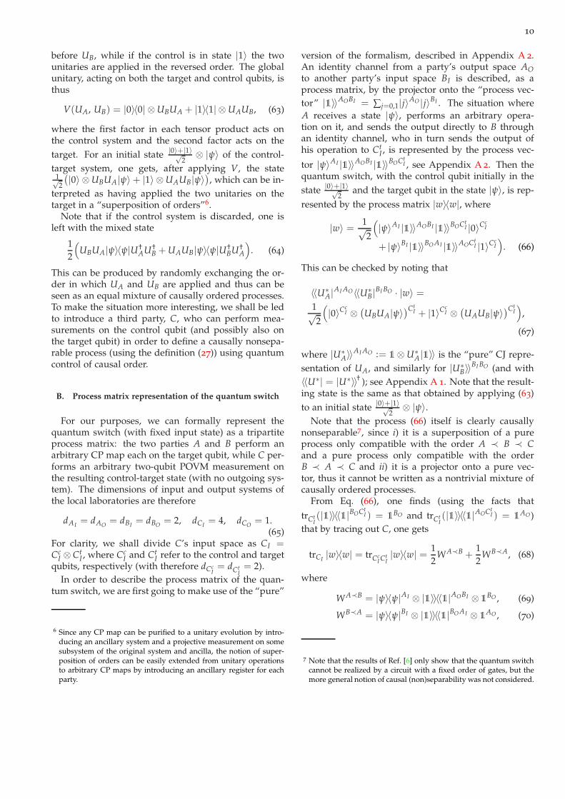
before UB, while if the control is in state |1〉 the twounitaries are applied in the reversed order. The globalunitary, acting on both the target and control qubits, isthus

V(UA, UB) = |0〉〈0| ⊗ UBUA + |1〉〈1| ⊗ UAUB, (63)

where the first factor in each tensor product acts onthe control system and the second factor acts on the

target. For an initial state |0〉+|1〉√2

⊗ |ψ〉 of the control-

target system, one gets, after applying V, the state1√2

(|0〉 ⊗ UBUA|ψ〉+ |1〉 ⊗ UAUB|ψ〉

), which can be in-

terpreted as having applied the two unitaries on thetarget in a “superposition of orders”6.

Note that if the control system is discarded, one isleft with the mixed state

12

(UBUA|ψ〉〈ψ|U†

AU†B + UAUB|ψ〉〈ψ|U†

BU†A

). (64)

This can be produced by randomly exchanging the or-der in which UA and UB are applied and thus can beseen as an equal mixture of causally ordered processes.To make the situation more interesting, we shall be ledto introduce a third party, C, who can perform mea-surements on the control qubit (and possibly also onthe target qubit) in order to define a causally nonsepa-rable process (using the definition (27)) using quantumcontrol of causal order.

B. Process matrix representation of the quantum switch

For our purposes, we can formally represent thequantum switch (with fixed input state) as a tripartiteprocess matrix: the two parties A and B perform anarbitrary CP map each on the target qubit, while C per-forms an arbitrary two-qubit POVM measurement onthe resulting control-target state (with no outgoing sys-tem). The dimensions of input and output systems ofthe local laboratories are therefore

dAI= dAO

= dBI= dBO

= 2, dCI= 4, dCO

= 1.(65)

For clarity, we shall divide C’s input space as CI =Cc

I ⊗ CtI , where Cc

I and CtI refer to the control and target

qubits, respectively (with therefore dCcI= dCt

I= 2).

In order to describe the process matrix of the quan-tum switch, we are first going to make use of the “pure”

6 Since any CP map can be purified to a unitary evolution by intro-ducing an ancillary system and a projective measurement on somesubsystem of the original system and ancilla, the notion of super-position of orders can be easily extended from unitary operationsto arbitrary CP maps by introducing an ancillary register for eachparty.

version of the formalism, described in Appendix A 2.An identity channel from a party’s output space AO

to another party’s input space BI is described, as aprocess matrix, by the projector onto the “process vec-tor” |1〉〉AOBI = ∑j=0,1|j〉AO |j〉BI . The situation whereA receives a state |ψ〉, performs an arbitrary opera-tion on it, and sends the output directly to B throughan identity channel, who in turn sends the output ofhis operation to Ct

I , is represented by the process vec-

tor |ψ〉AI |1〉〉AOBI |1〉〉BOCtI , see Appendix A 2. Then the

quantum switch, with the control qubit initially in the

state |0〉+|1〉√2

and the target qubit in the state |ψ〉, is rep-

resented by the process matrix |w〉〈w|, where

|w〉 = 1√2

(|ψ〉AI |1〉〉AOBI |1〉〉BOCt

I |0〉CcI

+ |ψ〉BI |1〉〉BO AI |1〉〉AOCtI |1〉Cc

I

). (66)

This can be checked by noting that

〈〈U∗A|AI AO〈〈U∗

B|BI BO · |w〉 =1√2

(|0〉Cc

I ⊗(UBUA|ψ〉

)CtI + |1〉Cc

I ⊗(UAUB|ψ〉

)CtI

),

(67)

where |U∗A〉〉

AI AO := 1⊗ U∗A|1〉〉 is the “pure” CJ repre-

sentation of UA, and similarly for |U∗B〉〉BI BO (and with

〈〈U∗| = |U∗〉〉† ); see Appendix A 1. Note that the result-ing state is the same as that obtained by applying (63)

to an initial state |0〉+|1〉√2

⊗ |ψ〉.Note that the process (66) itself is clearly causally

nonseparable7, since i) it is a superposition of a pureprocess only compatible with the order A ≺ B ≺ Cand a pure process only compatible with the orderB ≺ A ≺ C and ii) it is a projector onto a pure vec-tor, thus it cannot be written as a nontrivial mixture ofcausally ordered processes.

From Eq. (66), one finds (using the facts that

trCtI(|1〉〉〈〈1|BOCt

I ) = 1BO and trCt

I(|1〉〉〈〈1|AOCt

I ) = 1AO)

that by tracing out C, one gets

trCI|w〉〈w| = trCc

I CtI|w〉〈w| = 1

2WA≺B +

12

WB≺A, (68)

where

WA≺B = |ψ〉〈ψ|AI ⊗ |1〉〉〈〈1|AOBI ⊗ 1BO , (69)

WB≺A = |ψ〉〈ψ|BI ⊗ |1〉〉〈〈1|BO AI ⊗ 1AO , (70)

7 Note that the results of Ref. [6] only show that the quantum switchcannot be realized by a circuit with a fixed order of gates, but themore general notion of causal (non)separability was not considered.

11

are (bipartite) causally ordered process matrices;trCI

|w〉〈w| indeed describes the situation of Eq. (64).For some information-processing tasks, the quantum

switch is known to provide an advantage over causallyordered processes [7, 8], even when C ignores the tar-get system and only measures the control system. Wewill thus restrict our attention to witnesses of the formSCc

I ⊗ 1Ct

I , which can simplify the analysis and the ex-perimental implementation. The reduced process wewill be dealing with is the partial trace of the quantumswitch (66) over the target system:

Wswitch = trCtI|w〉〈w|. (71)

Note that the proof of causal nonseparability based onthe purity of the switch does not extend to the reducedswitch (71), since it is not an extremal process. Wewill therefore use the framework of causal witnesses toshow that the reduced switch is also causally nonsepa-rable.

V. WITNESSES FOR THE QUANTUM SWITCH

Since the quantum switch is a tripartite processwhere dCO

= 1, we can use definition (27) to study itscausal (non)separability. In this tripartite situation, wewill define causal witnesses to be the hermitian opera-tors S such that

tr[S Wsep] ≥ 0 (72)

for every causally separable processes Wsep in the coneWsep

3C . The set of causal witnesses is thus the cone dualto Wsep

3C , which we denote by S3C, or S3C,V when re-stricted to LV . The characterization of S3C is given bythe following theorem:

Theorem 3. A hermitian operator S ∈ AI ⊗ AO ⊗ BI ⊗BO ⊗ CI ⊗ CO with dCO

= 1 is a causal witness if and onlyif S can be written as

S = SPABC + S⊥

ABC = SPBAC + S⊥

BAC, (73)

where

SPABC ≥ 0, LA≺B≺C(S

⊥ABC) = 0, (74)

SPBAC ≥ 0, LB≺A≺C(S

⊥BAC) = 0, (75)

with LA≺B≺C and LB≺A≺C as defined in Subsection II B 3.

The proof is given in Appendix G. This characteriza-tion allows us to cast the problem of finding a witnessfor the quantum switch (or in fact for any process Wwith dCO

= 1) as an SDP problem analogous to (38):

min tr(SW)

s.t. S ∈ S3C,V , 1/dO − S ∈ W∗3C,V ,

(76)

where W∗3C,V := W∗

3C ∩ LV , with W∗3C the dual of the

cone W3C of (non-normalized) tripartite process matri-ces with dCO

= 1.Analogously to problems (38)–(39), the dual of (76)

writes

min tr[Ω]/dO

s.t. W + Ω ∈ Wsep3C , Ω ∈ W3C,

(77)

and the optimal values of (76) and (77) respect the dual-ity relation (40), which allows us to interpret − tr(S∗W)as generalised robustness also in this case. Further-more, (76) and (77) respect the assumptions of the Du-ality Theorem, and therefore SDP algorithms can findtheir optimal solutions efficiently. We shall, however,omit the proofs, as they are simply a slight modifica-tion of the ones already presented in Appendix E.

A. Optimal witness

To find the optimal generalised robustness witnessfor the quantum switch we need to solve SDP prob-lem (76) providing Wswitch from Eq. (71) as an argu-ment. Solving it using YALMIP and the solver MOSEKwe obtain a witness Soptimal numerically; the gener-alised robustness of the quantum switch is found to be

Rg(Wswitch) = − tr SoptimalWswitch ≈ 0.5454 . (78)

Later in this section we will compare this number tothat obtained from non-optimal witnesses. For this pur-pose, we shall use the amount of worst-case noise tol-erated by a witness, i.e., the amount of worst-case noisethat can be added to the quantum switch before the wit-ness can no longer detect its causal nonseparability. Itshould be clear that, when the said witness is optimal,this number reduces to the generalised robustness ofthe quantum switch.

B. Chiribella’s witness

In Ref. [7] Chiribella proposed an information-processing task for which the quantum switch had anadvantage over causally ordered processes. We want tounderstand what this advantage means, and how it re-lates to causal nonseparability. For that we shall presenta slightly modified version of his task and show how itcan be understood as a causal witness.

Our version of the task is as follows: Alice (party A)receives a qubit in her lab, applies a unitary UA to it,and sends it away. Bob (party B) receives a qubit in hislab, applies a unitary UB to it, and sends it away. Weassume that in each run of the experiment, UA and UB

12

either commute or anticommute. Charlie (party C) re-ceives a qubit in his lab, and makes a measurement onit to decide whether UA and UB commute or anticom-mute.

To construct a causal witness in relation to this task,we start with the Choi-Jamiołkowski representation ofthe actions of the parties: Alice applying a unitary UA,Bob applying a unitary UB, and Charlie obtaining the

result ± when measuring in the |±〉 = |0〉±|1〉√2

basis.

Using the CJ representations |U∗A〉〉 and |U∗

B〉〉 of UA andUB (see Appendix A 1), the corresponding operator is

GUA ,UB± = |U∗

A〉〉〈〈U∗A| ⊗ |U∗

B〉〉〈〈U∗B| ⊗ |±〉〈±| . (79)

The witness corresponding to the task is obtained byaveraging over the cases where Charlie obtains + whenAlice and Bob apply commuting unitaries, and thecases where Charlie obtains − when Alice and Bob ap-ply anticommuting unitaries:

GChiribella =12

∫dµ[ , ] G

UA ,UB+ +

12

∫dµ , G

UA ,UB− ,

(80)where dµ[ , ] is a measure over commuting unitaries, anddµ , is a measure over anticommuting unitaries (weassume here that the cases where UA and UB commuteand anticommute each appear with probability 1

2 ). Theprobability of success in this task when the parties areusing a strategy described by a process matrix W is then

psucc = tr[GChiribellaW] . (81)

It is easy to check that for any choice of measuresdµ[ , ], dµ , the probability of success is 1 when W =Wswitch. The maximal probability of success for causallyseparable processes, however, depends crucially on themeasures dµ[ , ] and dµ , . If we were to choose, for ex-ample, measures that only produce pairs of Pauli ma-trices, then there is a causally separable circuit8 that candecide the commutativity or anticommutativity withprobability 1.

To avoid this problem we will first choose measuresthat can produce any pair of commuting or anticom-muting unitaries (modulo global phases). Specifically,we choose the commuting measure dµ[ , ] to pick upcommuting unitaries of the form

UA = U

(1 00 eiθ1

)U† and UB = U

(1 00 eiθ2

)U†, (82)

where U is uniformly distributed according to the Haarmeasure, and θi are uniformly distributed in the inter-val [0, 2π]. For the anticommuting measure dµ , , we

8 One such circuit, described in Ref. [7], involves applying the Pauliunitaries to one half of a maximally entangled state and doing ameasurement in the Bell basis.

will use UA = VXV† and UB = VZV† , where V isalso a Haar-random unitary (and X and Z are the Paulimatrices)9.

With these measures GChiribella turns out to be a validcausal witness, as the maximal probability of successfor causally separable processes p

sepsucc is bounded below

one. To calculate it we need to solve the following SDPproblem:

max tr[GChiribellaW]

s.t. tr W = dO, W ∈ Wsep3C .

(83)

Solving it with YALMIP and MOSEK, we obtain

psepsucc ≈ 0.9288 . (84)

The amount of worst-case noise that GChiribella can tol-erate is 0.0766, which is much worse than the 0.5454tolerated by Soptimal.

An issue with GChiribella is that it would take an in-finite number of measurements to estimate each termof the sum in (80). Furthermore dµ[ , ] and dµ , werechosen arbitrarily, while it would be preferable to have ajustification for the choice of a particular measure. Bothproblems are solved by restricting the unitaries UA andUB to come from a finite set. In this way we only needperform a finite number of measurements to estimatethe witness, and it is possible to optimize the measuresover commuting and anticommuting unitaries throughSDP problems.

The best witness we found is obtained by choosingthe following ten unitaries:

G = 1, X, Y, Z,X + Y√

2,

X −Y√2

,

X + Z√2

,X − Z√

2,

Y + Z√2

,Y − Z√

2 (85)

(Y being the third Pauli matrix), and defining the wit-ness to be

Gfinite =10

∑i,j=1

q[ , ]ij G

Ui,Uj

+ + q , ij G

Ui,Uj

− , (86)

where Uk ∈ G, and q[ , ]ij , q

, ij are the input probability

distributions over commuting and anticommuting uni-

taries, normalised such that ∑i,j(q[ , ]ij + q

, ij ) = 1.

9 It turns out that with this choice of measures the witness GChiribellais the same as we would obtain by translating the task from Ref. [7]directly into the language of causal witnesses; the only difference,then, is that in [7] the witness was decomposed in terms of mea-surements and repreparations, whereas we decomposed it usingunitaries only.

13

To obtain the weights q[ , ]ij , q

, ij and p

sepsucc we solved an

SDP problem presented in Appendix H. We obtained

psepsucc ≈ 0.8690 , (87)

and tolerance to worst-case noise 0.1507, which ishigher than GChiribella’s 0.0766, but still lower thanSoptimal’s 0.5454.

We want to emphasize that the witnesses obtainedin this subsection are equivalent to the ones definedthrough (72) in the beginning of the present section– the only difference being the arbitary choice of thecausal bound being ≥ 0 vs ≤ p

sepsucc. More precisely, let

G be a witness such that

tr(G Wsep) ≤ psepsucc (88)

for every (normalised) causally separable Wsep and

T0 ≤ tr(G W) ≤ T1 (89)

for every (normalised) process matrix W. Then

S =1

psepsucc − T0

(p

sepsucc

1

dO− G

)(90)

is a valid generalised robustness witness. Furthermore,if S is the optimal witness for some process matrix Wthat saturates the upper bound tr(G W) = T1, it followsthat

Rg(W) = − tr[SW] =T1 − p

sepsucc

psepsucc − T0

. (91)

When G is either Gfinite or GChiribella, we have thatT0 = 0 and T1 = 1. And even though they are notoptimal witnesses for Wswitch, the relationship betweenp

sepsucc and resistance to worst-case noise is valid for

them, i.e., for both Gfinite and GChiribella the resistance toworst-case noise is equal to 1/p

sepsucc − 1, as given by (91).

VI. CAUSAL INEQUALITIES

The notion of causal separability considered aboverelies on the quantum description of the local laborato-ries. One may ask what are the constraints imposed bya definite causal structure regardless of the specific de-scription, or even the physics governing the devices per-forming the local operations. To study such restrictions,we will make use of so-called causal inequalities [13],which bound the possible correlations that can be estab-lished between events following a definite causal order.The violation of a causal inequality gives a stronger,device-independent signature of lack of causal orderthan the measurement of a witness. It is natural to askwhether it is possible to use the quantum switch to vio-late a causal inequality; we show below that this is notthe case.

A. Device-independent causal relations

We still consider a multipartite scenario in which a setof N parties AiN

i=1 are located in different, separatedlaboratories. Each party can perform operations andobtain measurement outcomes. Contrary to the previ-ous case however, we do not consider here any partic-ular physical description of what happens in each lab;the “settings” for the operations in the different labo-ratories and the measurement outcomes are labelled bysome classical variables xi and ai (with 1 ≤ i ≤ N), re-spectively; for simplicity we assume that the xi’s andai’s take a finite number of values. Defining the vectorof settings ~x = (x1, . . . xN) and the vector of outcomes~a = (a1, . . . , aN), the device-independent description ofthe correlations established in such an experiment is en-coded in the conditional probability P(~a|~x).

Causal inequalities [13] are constraints on P(~a|~x) de-rived from the assumption that there exists an under-lying causal structure defining the order between par-ties. To be more precise, let us represent the causalorder in which the parties act by a permutation σ, de-fined such that party i acts before party j if and only ifσ(i) < σ(j). This leads to a total ordering of the parties,namely Aσ(1) ≺ Aσ(2) ≺ . . . ≺ Aσ(N). We then say thata probability distribution P(~a|~x) is compatible with thecausal order σ if no party signals to those before her10,namely if for every i the marginal distribution

P(aσ(1), . . . , aσ(i)|~x) := ∑aσ(j)

j>i

P(~a|~x) (92)

does not depend on the inputs xσ(j) with j > i; i.e.,

P(aσ(1), . . . , aσ(i)|xσ(1), . . . , xσ(i), xσ(i+1), . . . , xσ(N))

= P(aσ(1), . . . , aσ(i)|xσ(1), . . . , xσ(i), x′σ(i+1), . . . , x′σ(N))

∀ xσ(j), x′σ(j) . (93)

A probability distribution that is compatible with atleast one causal order σ is said to be causally ordered.

More generally, we allow the parties to share ran-domness to agree on a specific order of sending signalsbetween them before the inputs of the game are given tothem. This allows for convex combinations of causallyordered probability distributions:

P(~a|~x) = ∑σ

qσ Pσ(~a|~x), qσ ≥ 0, ∑σ

qσ = 1 , (94)

where each Pσ is compatible with a fixed order σ. Theseare still not the most general correlations compatible

10 Note that this condition is strictly stronger than no-signalling toeach individual party, since it is possible to signal to a group ofparties without signalling to any individual party.

14

with the assumption of a definite causal structure, asone party could control the causal order of a set of par-ties in its future [19, 29, 30]. Correlations compatiblewith this most general scenario of definite causal or-der are called simply causal. In the bipartite case, theset of causal correlations forms a convex polytope, de-limited by a finite number of facets that define causalinequalities [31]. The explicit definition of causal corre-lations in the general N-partite case is, however, rathercumbersome, and for the purposes of this article it willbe enough to consider probability distributions of theform (94), which is a sufficient (although not necessary)condition for causal separability.

As causally separable processes can only generatecausal correlations, the violation of a causal inequalitycan also be used to detect the causal nonseparability ofa process. While causal witnesses are device-dependentand can only detect causal nonseparability if each partytrusts her operation’s implementation, causal inequali-ties are completely device-independent: even if each partydistrusts her laboratory, they can still detect causal non-separability from the statistics of their experimentaloutcomes, if those violate a causal inequality. Whilefor every causally nonseparable process there is causalwitness that will detect its nonseparability, there arecausally nonseparable processes cannot be used to vi-olate any causal inequalities: in the next subsectionwe will prove that the quantum switch provides suchan example. There is an analogy here with entangle-ment witnesses, which allow for a device-dependentway of detecting entanglement, and Bell inequalities,which provide a device-independent entanglement cer-tification – “nonlocality” [27]. The important differ-ence is that states violating Bell inequalities are physi-cally implementable, while no example of a physicallyimplementable process violating causal inequalities isknown.

B. Quantum control of orders and causal inequalities

One might first wonder if the quantum switch allowsfor a causal inequality violation between A and B (suchas the bipartite causal inequalities of Refs. [13, 31]); thisis however clearly not the case since, as pointed out be-fore, ignoring (i.e., tracing out) the third party C makesthe process matrix of the quantum switch causally sep-arable.

One might still hope that the quantum switch can beused to violate a tripartite inequality (see e.g. [30]), ex-plicitly involving party C; as it turns out, this is also im-possible, as a consequence of the following theorem11:

11 A similar conclusion based on the same example has been obtained

Theorem 4. Consider N+1 parties

A1, . . . , AN, C

withsettings x1, . . . , xN, z and outcomes a1, . . . aN , c. If themarginal distribution

P(~a|~x, z) := ∑c

P(~a, c|~x, z) (95)

is such that

1. P(~a|~x, z) = P(~a|~x) – i.e., it does not depend on z: C doesnot signal to any other (group of) parties;

2. P(~a|~x) = ∑σ qσ Pσ(~a|~x), where qσ ≥ 0, ∑σ qσ = 1, andthe probability distributions Pσ are causally ordered,

then the full (N+1)-partite probability distributionP(~a, c|~x, z) is causal.

Proof. Using Bayes’ rule and the assumptions of the the-orem, we can write

P(~a, c|~x, z) = P(~a|~x, z) P(c|~a,~x, z) (96)

= ∑σ

qσ Pσ(~a|~x) P(c|~a,~x, z) (97)

= ∑σ

qσ Pσ(~a, c|~x, z), (98)

where Pσ(~a, c|~x, z) := Pσ(~a|~x) P(c|~a,~x, z) is compatiblewith the order Aσ(1) ≺ . . . ≺ Aσ(N) ≺ C; this showsthat P(~a, c|~x, z) is causal.

To see that the correlations generated by the quantumswitch (Eq. (66)) respect assumptions 1. and 2. of theprevious theorem, let us calculate the marginal proba-bility distribution defined in Eq. (95) through the gen-eralized Born rule (3), when the three parties performoperations M

AI AO

a|x , MBI BO

b|y and MCIc|z:

P(a, b|x, y, z) = ∑c

tr[

MAI AO

a|x ⊗ MBI BO

b|y ⊗ MCI

c|z · |w〉〈w|]

= tr[

MAI AO

a|x ⊗ MBI BO

b|y ⊗(

∑c

MCI

c|z)· |w〉〈w|

]. (99)

Since the third party C has no output space (dCO= 1),

then for any instrument MCI

c|z we have ∑c MCI

c|z = 1CI ,

so that

P(a, b|x, y, z) = tr[

MAI AO

a|x ⊗ MBI BO

b|y · WAB]

(100)

with

WAB := trCI|w〉〈w| . (101)

This implies that P(a, b|x, y, z) does not depend on z,as required. As argued before, tracing out C from

by Oreshkov and Giarmatzi independently of the other authors ofthis paper and is presented in Ref. [19]

15

the process matrix representing the quantum switchleads to a causally separable process matrix of the formWAB = 1

2WA≺B + 12WB≺A with causally ordered pro-

cess matrices WA≺B and WB≺A, which can only gen-erate causally ordered probability distributions PA≺B

and PB≺A. Hence, P(a, b|x, y, z) can be decomposed as12 PA≺B(a, b|x, y, z) + 1

2 PB≺A(a, b|x, y, z), so that the sec-ond assumption of Theorem 4 is also satisfied.

Therefore, the quantum switch represents an exam-ple of a causally nonseparable process that can onlygenerate causal correlations, and hence cannot be usedto violate any causal inequality12. It is noteworthy thatall the examples of causally nonseparable processes forwhich a physical interpretation is known, includingthose generated by space-time superpositions [32], fallinto this category. This raises the question of whethercausally nonseparable processes that do violate causalinequalities can be physically implemented at all.

VII. CONCLUSION

The process matrix formalism was originally con-ceived as a rather speculative extension of quantum me-chanics to possibly include the indefinite causal struc-tures expected in a quantized theory of gravity [10].The results of this work show that, in fact, it is a natu-ral framework to study a class of quantum resourceswhich cannot be captured by the circuit model, butnonetheless are physically realizable and can providepowerful computational advantages. We have shownthat the quantum switch, a recently demonstrated re-source for quantum computation, can be convenientlyrepresented as a causally non-separable process matrix.We have also presented causal witnesses that can verifythe causal nonseparability of the switch. As they onlyrequire performing unitaries in a “superposition of or-der” and a final measurement of a control qubit, suchwitnesses can be easily implemented in quantum-opticssetups, as the one employed in Ref. [9].

The theory of causal witnesses developed here hasclose resemblances with the theory of entanglementwitnesses. In both cases, one is interested in findingways to certify that a resource is outside some convexset, the set of separable states in the latter case, thatof causally nonseparable process matrices in the for-mer case. Following this analogy, causal inequalitiescan be seen as the counterpart to the Bell inequalities,as they both provide device-independent tests regard-ing the existence of some classical variable: local hid-den variables for measurement outcomes in one case,

12 Note that Theorem 4 implies that this is also true for the N-partitegeneralization of the quantum switch defined in [8].

classical variables determining the causal order in theother. A significant difference between the two frame-works is that the problem of determining causal sepa-rability can be solved numerically with efficient algo-rithms, whereas characterizing entanglement has beenproven to be an NP-hard problem [33].

As one could expect from the analogy with entangle-ment, there exist causally nonseparable processes thatcannot violate causal inequalities. What is striking, inthe case of process matrices, is that a physical interpre-tation is known only for resources in this category. Asone of the main open problems in this field is the char-acterization of physical process matrices, it is tempt-ing to speculate whether the (im)possibility to violatecausal inequalities could provide a useful guidance inthis respect.

Acknowledgements

We thank Michal Sedlák for useful discussions. Weacknowledge support from the European Commissionproject RAQUEL (No. 323970); the Austrian ScienceFund (FWF) through the Special Research ProgramFoundations and Applications of Quantum Science (Fo-QuS), the doctoral programme CoQuS, and IndividualProject (No. 2462); FQXi; the John Templeton Founda-tion; the Templeton World Charity Foundation (grantTWCF 0064/AB38); the French National ResearchAgency through the ‘Retour Post-Doctorants’ program(ANR-13-PDOC-0026); and the European Commissionthrough a Marie Curie International Incoming Fellow-ship (PIIF-GA-2013-623456).

Appendix A: Details of the formalism

Here we explore in more details the properties of theChoi-Jamiołkowski (CJ) isomorphism and of the pro-cess matrix formalism. Note that other existing def-initions of the CJ isomorphism differ by a transposi-tion or a partial transposition from the one given here,which follows the convention in [13] and allows a directidentification of non-signaling processes with quantumstates.

1. Choi-Jamiołkowski isomorphism

a. Pure CJ isomorphism. It is convenient to distin-guish two versions of the CJ isomorphism: one formaps over density matrices and one for linear opera-tors on pure state. The latter – the “pure CJ isomor-phism” – can be represented via the “double-ket” nota-tion [34, 35]. For a linear operator A : HAI → HAO , we

16

define13

|A∗〉〉AI AO := 1⊗ A∗|1〉〉, (A1)

where |1〉〉 ≡ |1〉〉AI AI := ∑j|j〉AI ⊗ |j〉AI ∈ HAI ⊗HAI

(with also, of course, the usual notation 〈〈1| = |1〉〉†),and the complex conjugation ∗ is defined with respectto the chosen orthonormal basis |j〉AI of HAI . Theinverse map is given by

A|ψ〉 =[〈ψ|AI ⊗ 1

AO · |A∗〉〉AI AO]∗

. (A2)

We say that |A∗〉〉 is the CJ representation (or CJ vector)of A. The cumbersome complex conjugation in the defi-nition allows us to have a simpler representation for theprocess matrix.

b. Maximally entangled states and unitaries. Con-sider here the case where the input and output spaceshave equal dimensions, dAI

= dAO. The state obtained

by applying a local unitary to one subsystem of a max-imally entangled state is also maximally entangled. inreverse, it is possible to generate any (bipartite) maxi-mally entangled state by applying a local unitary to onesubsystem of a reference maximally entangled state.Therefore, the CJ vector |U∗〉〉AI AO = 1⊗ U∗|1〉〉 is max-imally entangled if and only if U is a unitary. More explic-itly, an operator

U = ∑jk

ujk |j〉〈k| (A3)

is unitary if and only if ∑l ujlu∗kl = ∑l u∗

lkul j = δj,k forall j, k. One can check that this is also a necessary andsufficient condition for which

|U∗〉〉AI AO = ∑jk

u∗jk|k〉AI |j〉AO (A4)

is maximally entangled.

c. Measurement-preparation. Another useful linearoperator is |ψ〉〈φ|, which describes the observation ofan outcome |φ〉 in a projective measurement, followedby the repreparation of a state |ψ〉. Plugging this intothe definition (A1), we find the CJ representation

∣∣ (|ψ〉〈φ| )∗⟩⟩AI AO = |φ〉AI ⊗ (

|ψ〉∗)AO . (A5)

Reciprocally, every pure product CJ vector represents ameasurement-preparation operation.

An important particular case is when |ψ〉 = |φ〉,which corresponds to the ideal non-demolition vonNeumann measurement:

∣∣ (|φ〉〈φ| )∗⟩⟩AI AO = |φ〉AI ⊗ (

|φ〉∗)AO . (A6)

13 Superscripts on CJ vectors and CJ matrices indicate the systemsthey refer to (they may be omitted when the context makes it clearenough).

d. Mixed CJ operators. For the general case of a lin-ear map MA : AI → AO, we define the CJ isomorphismas

MAI AO :=[I ⊗MA(|1〉〉〈〈1|)

]T. (A7)

It is easy to verify that the definition (A7) reducesto (A1) for operators of the form MA(ρ) = AρA†, i.e.that, in such a case,

M = |A∗〉〉〈〈A∗| (A8)

(with |A∗〉〉 ≡ |A∗〉〉AI AO and 〈〈A∗| = |A∗〉〉†).According to Choi’s theorem [36], a linear map MA :

AI → AO is CP if and only if its CJ matrix is posi-tive semidefinite, MAI AO ≥ 0. A characterization of thetrace-preserving condition can be found using the in-verse CJ isomorphism,

MA(ρ) =[

trAI[ρAI ⊗ 1

AO · MAI AO ]]T

. (A9)

By taking the trace of both sides of the equation, it canbe readily verified that the map MA is trace-preservingif and only if

trAOMAI AO = 1

AI . (A10)

Note that a CP map can be part of an instrument onlyif it is trace-non-increasing, a condition that translates to

1AI − trAO

MAI AO ≥ 0 . (A11)

A useful example is the CPTP map MA(σ) = ρ tr σ,which corresponds to the preparation of a (normalized)state ρ independently of the input state σ. Its CJ repre-sentation is found to be

MAI AO = 1AI ⊗ (ρT)AO . (A12)

A second relevant case is the CP (not trace-preserving)map that gives the probability of observing a POVMelement E in a measurement: MA(ρ) = tr[Eρ] (heredAO

= 1). Its CJ representation is simply

MAI = EAI . (A13)

Finally, the situation where a POVM element E is mea-sured on the state σ in AI and a state ρ is preparedin AO corresponds to the CP map MA(σ) = ρ tr[Eσ],which has CJ representation

MAI AO = EAI ⊗ (ρT)AO . (A14)

2. Process matrices

Here we discuss in more detail some examples andproperties of process matrices.

17

a. Quantum states. Consider a bipartite processmatrix of the form

WAI AOBI BO = ρAI BI ⊗ 1AOBO . (A15)

According to the generalized Born rule, Eq. (3), theprobability for the two parties A and B to perform tracenon-increasing CP maps with CJ matrices MAI AO andMBI BO , respectively, is given by

P(

MAI AO , MBI BO)= tr

[(MAI AO ⊗ MBI BO

)W

],

= tr[(

EAI ⊗ EBI)ρAI BI

], (A16)

where EAI := trAOMAI AO and EBI := trBO

MBI BO .These operators are positive semidefinite and, becauseof Eq. (A11), they can be completed to form a POVM.Thus Eq. (A16) corresponds to the probability of ob-serving the POVM element EAI ⊗ EBI given the stateρAI BI ; in other words, the process matrix (A15) de-scribes a bipartite state. Notice that a process matrixof this form does not allow signalling in either direc-tion and therefore, being compatible with both A ≺ Band B ≺ A, it is causally separable. This is irrespec-tive of the state ρ, which can be entangled or separa-ble. Note also the difference between the process ma-trix (A15) and the CJ representation of state prepara-tion, Eq. (A12).

b. Channels. Consider a bipartite situation where aparty A only performs state preparations, while the sec-ond party B only performs measurements. In this case,the local laboratory of A is characterized by a trivial in-put space, dAI

= 1, while B has a trivial output space,dBO

= 1. The process matrix shared by A and B, whichrepresents here a quantum channel, is then defined onthe space AO ⊗ BI ∋ W. The probability that B observesa POVM element E when A prepares a state ρ is givenby

P(E|ρ) = tr[(

ρT)AO⊗ EBI · WAOBI

], (A17)

where we used (A12) and (A13) for the local op-erations. This is equivalent to saying that B mea-

sures E in the state trAO

[(ρT

)AO ⊗ 1BI · WAOBI

]=

[trAO

[ρAO ⊗ 1

BI ·(WT

)AOBI]]T

. Comparing this with

the inverse CJ transformation (A9), we find that the pro-cess matrix W corresponds to a channel with CJ repre-sentation WT . In other words, a channel C from AO toBI is represented by the process matrix

WAOBI = I ⊗ C(|1〉〉〈〈1|) (A18)

(with here |1〉〉 ≡ |1〉〉AO AO). Note that the CJ represen-tation of a channel, Eq. (A7), differs by a transpositionfrom the corresponding process matrix (A18).

c. Reduced process matrices. Given a multipartite

process W = WA1I A1

O...ANI AN

O and a CPTP map for the j-

th party with CJ matrix MAjI A

jO , we define the reduced

process matrix for the remaining N − 1 parties, given

MAjI A

jO , as

W(MAjI A

jO)

:= trA

jI A

jO

[(1

A1I A1

O⊗ . . . MAjI A

jO⊗ . . .1AN

I ANO)·W

]. (A19)

With the usual generalized Born rule (3), the reducedprocess matrix gives the probability for the remainingN − 1 parties to measure arbitrary CP maps, given that

the j-th party performs MAjI A

jO . The explicit depen-

dence of W on MAjI A

jO accounts for the possibility of sig-

nalling: the remaining parties observe different proba-bility distributions depending on the choice of CPTPmap performed by party j. As an example, consider aprocess matrix of the form (A18). If A prepares a stateρ, the reduced process matrix for B is

WBI (ρ) = trAO

[(ρT

)AO⊗ 1BI · WAOBI

]

= ∑jk

〈k|ρT|j〉 C(|j〉〈k|) = C(ρ). (A20)

Thus, for a process that represents a channel from A toB, the reduced process for B, given that A prepares ρ, issimply the channel applied to ρ, as should be expected.

d. Pure process matrices. In some cases, the processmatrix turns out to be a rank-one projector: W = |w〉〈w|for some “process vector” |w〉. If the CJ operators rep-resenting the local operations are also rank-one pro-jectors, as is the case for unitaries and projective mea-surements followed by pure repreparations, it is conve-nient to work at the level of vectors and of probabilityamplitudes: given the local operations A1, . . . , AN rep-

resented by the CJ vectors |A∗1〉〉

A1I A1

O , . . . , |A∗N〉〉AN

I ANO ,

the overall probability amplitude is given (up to globalphase, which we choose to be 0) by

〈〈A∗1 |A

1I A1

O ⊗ · · · ⊗ 〈〈A∗N|A

NI AN

O · |w〉A1I A1

O...ANI AN

O . (A21)

The probability is then obtained as the modulus squareof the amplitude and conforms to the general expres-sion (3). Given that party j performs the unitary Uj, thereduced process is clearly given by the partial scalarproduct

1A1

I A1O ⊗ . . . 〈〈U∗

j |AjI A

jO ⊗ . . .1AN

I ANO · |w〉A1

I A1O ...AN

I ANO .

(A22)The process matrix describing a unitary channel U

from AO to BI is of particular interest. Using (A18), wefind that it is given by

|w〉AOBI = 1⊗ U|1〉〉 = |U〉〉AOBI . (A23)

18

Note again the difference between this expression andthe CJ representation (A1). Generalizing this to a se-quence of parties A1, . . . , AN , with the output of party jconnected to the input of party j + 1 via the unitary Uj,we find

|w〉A1O...AN

I = |U1〉〉A1O A2

I ⊗ · · · ⊗ |UN〉〉AN−1O AN

I . (A24)

Appendix B: Valid process matrices

The conditions for an operator W ∈ AI ⊗ AO ⊗BI ⊗ BO to be a valid process matrix were first foundin Ref. [13], where they were formulated in a basis-dependent way. Here we derive the equivalent charac-terization of valid process matrices given in Eqs. (4)–(6);we formulate it in a basis-independent way, which wefind to be more convenient for our purposes.

We present below the derivation in the bipartite case,and also write explicitly, for ease of reference, the char-acterization in the tripartite case. The N-partite casefollows from a straightforward generalization.

1. Bipartite process matrices

Recall that a given operator W ∈ AI ⊗ AO ⊗ BI ⊗ BO

is a valid process matrix if and only if it yields, throughthe generalized Born rule (3), only well-defined proba-bilities – that is, the probabilities must be non-negativeand must sum up to 1.

Non-negativity. As recalled previously, a map iscompletely positive if and only if its CJ representationis positive semidefinite. Including the possibility thatA and B’s operations involve interactions with a (pos-sibly entangled) ancillary system in a state ρA′

I B′I , the

non-negativity of probabilities is thus equivalent to14

tr[(

MA′I AI AO ⊗ MB′

I BI BO) · (ρA′

I B′I ⊗ WAI AOBI BO

)] ≥ 0

∀ MA′I AI AO ≥ 0 , MB′

I BI BO ≥ 0 , ρA′I B′

I ≥ 0 . (B1)

For the case where the ancillary spaces A′I and

B′I are isomorphic to AI ⊗ AO, and MA′

I AI AO andρA′

I B′I are both projectors onto the maximally entangled

state |1〉〉AI AO/AI AO := ∑j,k|j, k〉AI AO ⊗ |j, k〉AI AO (where

|j, k〉AI AO is an orthonormal basis of HAI ⊗ HAO),we find that the trace in (B1) is equal to tr[MB′

I BI BO ·

14 Note that ignoring the possibility of an ancillary system, one wouldonly find that W must be “positive on pure tensors” (with respectto the partition AI AO/BI BO) – a class strictly larger than positivesemidefinite matrices [37].

WAI AOBI BO ]. Requiring that its value is non-negativefor all MB′

I BI BO ≥ 0 implies that W must be positivesemidefinite.

Reciprocally, W ≥ 0 clearly implies that (B1) is satis-fied. Hence, the non-negativity of probabilities is equiv-alent to W being positive semidefinite, Eq. (4).

Normalization. The fact that probabilities must sumup to 1 for all instruments is equivalent to the constraintthat the probability of realization of any CPTP map is1. Now, recall that a CP map MA : AI → AO is trace-preserving if and only if its CJ matrix MAI AO satisfiestrAO

MAI AO = 1AI – or equivalently, using the nota-

tion of Eq. (12), AOMAI AO = 1

AI AO/dAO. Ignoring here

for simplicity the possible use of an ancillary system(which leads to the same conclusion15), the normaliza-tion of probabilities is thus equivalent to

tr[(

MAI AO ⊗ MBI BO)· WAI AOBI BO

]= 1

∀ MAI AO ≥ 0 , MBI BO ≥ 0 ,

s.t. AOMAI AO = 1

AI AO/dAO, BO

MBI BO = 1BI BO /dBO

.(B2)

First of all, note that the positivity of MAI AO andMBI BO is irrelevant here, since the set of positivesemidefinite operators is a full dimensional subset ofthe space of hermitian operators16. The only relevantconditions are the normalization constraints. Definingthe maps [1−AO]

M = M − AOM and [1−BO]

M = M −BO

M, and noting that for any hermitian operators x andy, the operators [1−AO]

x + 1/dAOand [1−BO]

y + 1/dBO

15 Taking into account a possible ancillary state ρA′I B′

I , the same rea-soning as below leads to Eqs. (B4) and (B15), with W replaced byρA′

I B′I ⊗ W AI AOBI BO (and where the definitions of the maps LA and

LB should include the ancillary systems B′I and A′

I , resp.), which

must hold for all ρA′I B′

I such that tr ρA′I B′

I = 1. One can easily checkthat these are indeed equivalent to (B4) and (B15) in their originalform.

16 More precisely: for any hermitian operator MAI AO , there alwaysexists α > 0 such that MAI AO + α1

AI AO /dAO≥ 0. Assuming

that AOMAI AO = 1

AI AO /dAO, one can thus decompose MAI AO as

MAI AO = (α+1) MAI AO+ − α M

AI AO− , with M

AI AO+ = 1

α+1 (MAI AO +

α1AI AO /dAO

) ≥ 0 and MAI AO− = 1

AI AO /dAO≥ 0 satisfying

AOM

AI AO+ = AO

MAI AO− = 1

AI AO /dAO. Similarly, any hermitian

operator MBI BO such that BOMBI BO = 1

BI BO /dBOcan be decom-

posed as MBI BO = (β+1) MBI BO+ − β M

BI BO− , with M

BI BO+ ≥ 0,

MBI BO− ≥ 0 and BO

MBI BO+ = BO

MBI BO− = 1

BI BO /dBO. Note that

the four pairs (MAI AO± , M

BI BO± ) satisfy the assumptions of Eq. (B2),

and therefore tr[(

MAI AO± ⊗ M

BI BO±

)· W AI AO BI BO

]= 1. Expanding

tr[(

MAI AO ⊗ MBI BO)· W AI AO BI BO

]using the decomposition just

constructed, we find that its value is also 1. Hence, if Eq. (B2) holds,then it also holds without the positivity constraints on MAI AO andMBI BO ; the converse is of course trivially true.

19

satisfy the above normalization constraints (where fromnow on we are omitting the superscripts to reduce clut-tering), we find that Eq. (B2) is equivalent to

tr[(

[1−AO]x + 1/dAO

)⊗

([1−BO]

y + 1/dBO

)W

]= 1

∀ x, y . (B3)

For x = y = 0, this yields the normalization conditionof Eq. (5),

tr[W] = dAOdBO

. (B4)

For y = 0 and x = 0, respectively, this in turn implies

tr[(

[1−AO]x ⊗ 1

)W

]= 0 ∀ x , (B5)

tr[(

1⊗ [1−BO]y)

W]= 0 ∀ y , (B6)

which then imply

tr[(

[1−AO]x ⊗ [1−BO]

y)

W]= 0

∀ x, y . (B7)

Reciprocally, Eqs. (B4)–(B7) clearly imply (B3), so thatthese are equivalent to Eq. (B2).

Thinking of the trace as the Hilbert-Schmidt innerproduct

〈M, W〉 = tr[M · W]

(for hermitian operators M, W) and noting that themaps [1−AO]

· and [1−BO]· are self-dual, the condi-

tions (B5)–(B7) are equivalent to

[1−AO]

(trBI BO

W)= 0, (B8)

[1−BO]

(trAI AO

W)= 0, (B9)

[1−AO][1−BO]W = 0, (B10)

which we can rewrite as

BI BOW = AOBI BO

W , (B11)

AI AOW = AI AOBO

W , (B12)

W = BOW + AO

W − AOBOW , (B13)

which are conditions (9)–(11).Note that each condition (B8)–(B10) defines a linear

subspace, and the intersection of these three linear sub-spaces is the smallest subspace that contains all validbipartite process matrices, which we denote by17

LV =

W ∈ AI⊗AO⊗BI⊗BO |W = LV(W)

, (B14)

17 Note that although we do not write that explicitly, the projectorswe define below (e.g. LV), and of course the subspaces they define(e.g. LV), depend on the number of parties N.

The projector onto this subspace, LV , shall be used quiteoften in the paper, so it is useful to find an explicit ex-pression for it. To do that, first we rewrite conditions(B11)–(B13) explicitly as projections onto subspaces, i.e.,as

W = LA(W) , W = LB(W) , W = LAB(W) , (B15)

where the projectors LA, LB, and LAB are given by

LA(W) = W − BI BOW + AOBI BO

W , (B16)

LB(W) = W − AI AOW + AI AOBO

W , (B17)

LAB(W) = BOW + AO

W − AOBOW , (B18)

Since the three projectors above commute, the projec-tor onto the intersection of their subspaces LV is givensimply by the composition of LA, LB, and LAB, i.e.,

LV(W) = LA LB LAB(W), (B19)

which, after simplification, can be written as

LV(W) = AOW + BO

W − AOBOW

− BI BOW + AOBI BO

W

− AI AOW + AI AOBO

W (B20)

Summing up, we conclude that an operator W ∈AI ⊗ AO ⊗ BI ⊗ BO is a valid bipartite process matrixif and only if W ≥ 0, tr W = dAO

dBO, and W = LV (W),

as in Eqs (4)–(6).

2. Tripartite process matrices

A similar reasoning leads to the conclusion that anoperator W ∈ AI ⊗ AO ⊗ BI ⊗ BO ⊗ CI ⊗ CO is a validtripartite process matrix if and only if W ≥ 0, tr W =dAO

dBOdCO

, and

W = LA(W) , W = LB(W) , W = LC(W) ,

W = LAB(W) , W = LAC(W) , W = LBC(W) ,

W = LABC(W) , (B21)

where the maps LA, LB, LC, LAB, LAC, LBC, and LABC

are now commuting projectors onto linear subspaces ofAI ⊗ AO ⊗ BI ⊗ BO ⊗ CI ⊗ CO, defined by

LA(W) = [1−(1−AO)BI BOCI CO]W ,

LB(W) = [1−(1−BO)AI AOCI CO]W ,

LC(W) = [1−(1−CO)AI AOBI BO]W ,

LAB(W) = [1−(1−AO)(1−BO)CICO]W ,

LAC(W) = [1−(1−AO)(1−CO)BI BO]W ,

LBC(W) = [1−(1−BO)(1−CO)AI AO]W ,

LABC(W) = [1−(1−AO)(1−BO)(1−CO)]W ,

20

where we used the shorthand notation

[∑X αXX]W = ∑X

αX · XW (B22)

for a sum over products of subsystems X with coeffi-cients αX (and with 1W := W).

The constraints in (B21) are equivalent to

W = LV(W) , (B23)

where the map LV is obtained here by composing the 7

maps LA , LB, LC, LAB, LAC, LBC, and LABC. One findsin this tripartite case, after simplification,

LV(W) = [1−(1−AO+AI AO)(1−BO+BI BO)(1−CO+CI CO)

+ AI AOBI BOCI CO

]W ,

(B24)

which defines a projector onto the linear subspace

LV =

W ∈ AI⊗AO⊗BI⊗BO⊗CI⊗CO |W = LV(W)

.(B25)

3. N-partite process matrices

The generalization to the N-partite case is ratherstraightforward. We find that an operator W ∈ A1

I ⊗A1

O ⊗ . . . ⊗ ANI ⊗ AN

O is a valid N-partite process matrixif and only if W ≥ 0, tr W = dA1

O. . . dAN

O, and for all

2N − 1 non-empty subsets X of 1, . . . , N,

W = LX (W) := [1−∏i∈X (1−Ai

O) ∏i/∈X AiI Ai

O

]W . (B26)

Note that the 2N − 1 maps LX are commuting projec-tors onto linear subspaces of A1

I ⊗ A1O ⊗ . . .⊗ AN

I ⊗ ANO .

The constraints (B26) are equivalent to

W = LV(W) , (B27)

where the map LV is obtained this time by composingthe 2N − 1 maps LX . More explicitly, one finds in theN-partite case the general expression

LV(W) = [1 − ∏i(1−Ai

O+AiI Ai

O) + ∏i AiI Ai

O

]W , (B28)

which again defines a projector onto the linear subspace

LV =

W ∈ A1I ⊗ A1

O ⊗ . . . ⊗ ANI ⊗ AN

O | W = LV(W)

.(B29)

Proof. For any subset X of 1, . . . , N, define PX =∏i∈X (1− Ai

O) ∏i/∈X AiI Ai

O. For X 6= X ′, note that thereexists (at least one) i0 such that the product PX PX ′ con-tains the factor (1− A

i0O)A

i0I A

i0O. Now,

[(1−Ai0O )A

i0O ]

W = 0,

so that [PX PX ′ ]W = 0.

Developing LV , we thus find LV(W) =

[∏X 6=∅(1−PX )]W = [1−∑X 6=∅ PX ]W = [1−∑X PX+∏i AiI Ai

O]W.

Now, one can write ∑X PX = ∑1k1=0 . . . ∑

1kN=0(1 −

A1O)

k1(A1I A1

O)1−k1 . . . (1 − AN

O )kN (ANI AN

O )1−kN =

∏i ∑1ki=0(1 − Ai

O)ki(Ai

I AiO)

1−ki = ∏i(1 − AiO + Ai

I AiO),

from which Eq. (B28) follows.

Appendix C: Characterization of bipartite causal witnesses

To characterize below the set of causal witnesses inthe bipartite case, we shall make use of some basic def-initions and facts from convex analysis, which we statehere without any proof; the interested reader can findthem for instance in Sections 2, 14 and 16 of Ref. [21]18.

Let E be a vector space equipped with an inner prod-uct 〈·, ·〉, and let E′ be the space of all linear functionalson E. In the finite-dimensional case that interests us, E′

is isomorphic to E.

1. A subset K of E is a convex cone if and only if forevery x, y ∈ K we also have that λx + µy ∈ K, forany λ, µ > 0.

2. Let K ⊆ E be a convex cone. Then its dual coneK∗ ⊆ E′ is defined as

K∗ = x∗ ∈ E′ | 〈x∗, x〉 ≥ 0 ∀x ∈ K . (C1)

3. The dual of a linear subspace L ⊆ E is its orthog-onal complement:

L∗ = L⊥ = x∗ ∈ E′ | 〈x∗, x〉 = 0 ∀x ∈ L. (C2)

4. Let K1,K2 ⊆ E be closed convex cones that con-tain the origin. Then

[conv(K1 ∪K2)]∗ = K∗

1 ∩K∗2 , (C3a)

(K1 ∩K2)∗ = conv(K∗

1 ∪K∗2) , (C3b)

where conv denotes the convex hull.

We shall furthermore use below the following char-acterization of bipartite causally separable process ma-trices:

Lemma 5. A given matrix W ∈ AI ⊗ AO ⊗ BI ⊗ BO is avalid causally separable process matrix if and only if tr W =dO, W ∈ LV (i.e., it satisfies Eqs. (9)–(11)), and it can bewritten as

W = WA≺B + WB≺A (C4)

with WA≺B ≥ 0 , WA≺B = BOWA≺B , (C5)

WB≺A ≥ 0 , WB≺A = AOWB≺A . (C6)

18 Note a difference in language. This reference uses the polar coneK instead of the dual K∗ . They are simply related by K = −K∗.

21

Proof. The “only if” direction is straightforward (simplyreplace q WA≺B → WA≺B and (1−q)WB≺A → WB≺A togo from (18) to (C4), so that WA≺B and WB≺A in (C4)are not normalized).

To see that the converse also holds, first note thatWA≺B ≥ 0 and WB≺A ≥ 0 imply that W ≥ 0, sothat W is indeed a valid process matrix. Note further-more that WB≺A = AO

WB≺A implies that BI BOWB≺A =

AOBI BOWB≺A, i.e., that WB≺A satisfies (9). Since W ∈ LV

also satisfies (9), so does WA≺B = W − WB≺A. Sim-ilarly, WA≺B = BO

WA≺B, together with the assump-tion that W ∈ LV , implies that both WA≺B and WB≺A

satisfy (10). Lastly, WA≺B = BOWA≺B and WB≺A =

AOWB≺A directly imply that both WA≺B and WB≺A sat-

isfy (11). All in all, this shows that WA≺B and WB≺A

are, up to normalization (which can easily be dealt withas above so as to recover the form (18)), valid causallyordered process matrices.

We are now in a position to prove Theorem 1:

Proof of Theorem 1. We want to characterize the set of allhermitian operators S ∈ AI ⊗ AO ⊗ BI ⊗ BO such that

tr[SWsep] ≥ 0 (C7)

for all causally separable process matrices Wsep. Notethat the condition tr[Wsep] = dO is not relevant forthe characterization of the witnesses, so we shall liftit. Without this restriction the set of (non-normalized)causally separable process matrices becomes a convexcone, which we denote by Wsep. If we consider the du-ality relations with respect to the Hilbert-Schmidt innerproduct in the space AI ⊗ AO ⊗ BI ⊗ BO, then the con-vex cone of causal witnesses S is the dual cone of Wsep.To characterize it we are going to use the representationof Wsep that follows from Lemma 5:

Wsep = conv[(P ∩ LBO

) ∪ (P ∩ LAO)] ∩LV , (C8)

where P is the self-dual cone of positive semidefinitematrices and LBO

and LAOare the linear subspaces

LBO= W | W = BO

W, (C9)

LAO= W | W = AO

W, (C10)

and with LV defined in Eq. (B14). Their orthogonalcomplements within the subspace AI ⊗ AO ⊗ BI ⊗ BO

are simply given by

L⊥BO

= S | BOS = 0, (C11)

L⊥AO

= S | AOS = 0, (C12)

L⊥V = S | LV(S) = 0. (C13)

Taking then the dual of Wsep using the duality rela-tions (C2)–(C3), we get that the cone of causal witnessesis

S = conv[[(P ∩ LBO

)∗ ∩ (P ∩ LAO)∗] ∪ L⊥

V

]. (C14)

Focusing on (P ∩ LBO)∗, using again the duality rela-

tions (C2)–(C3), we see that

(P ∩ LBO)∗ = conv(P ∪L⊥

BO)

= S+ + S0 | S+ ≥ 0, BOS0 = 0

= S | BOS ≥ 0, (C15)

where the last equality is stating the fact that S = S+ +S0 with S+ ≥ 0 and BO

S0 = 0 if and only if BOS ≥ 0. To

see that this is true, let S be such that BOS ≥ 0. Define

then S+ = BOS and S0 = S − BO

S. Then S = S+ + S0,S+ ≥ 0 by assumption, and BO

S0 = 0 since the mapBO· is a projector. To prove the other direction, let S =

S+ + S0 with S+ ≥ 0 and BOS0 = 0. The map BO

· beingpositive, it follows that BO

S = BOS+ ≥ 0.

Similarly,

(P ∩ LAO)∗ = S | AO

S ≥ 0. (C16)

Putting Eqs. (C14)–(C16) together, we see that a causalwitness can be written as S = SP + S⊥ with BO

SP ≥0, AO

SP ≥ 0, and LV(S⊥) = 0.

Appendix D: Explicit positive semidefinite constraints

For the convenience of the reader, we present the SDPproblems (38) and (39) with all conic constraints rewrit-ten in terms of the positive semidefinite cone, to facil-itate implementation. To rewrite (38), we need a char-acterisation of the cones SV and W∗

V . The first one isgiven by Corollary 2. The second one is obtained asfollows: since W = P ∩ LV , we have that

W∗V = W∗ ∩LV (D1)

= (P ∩ LV)∗ ∩LV (D2)

= conv(P ∪ L⊥V ) ∩ LV (D3)

= LV (ΣP)|ΣP ≥ 0 , (D4)

where Equation (D4) follows from an argument analo-gous to the one used to derive Corollary 2.

With this characterisation, the SDP problem (38) thenbecomes

min tr(SW)

s.t. S = LV(SP) , AOSP ≥ 0 , BO

SP ≥ 0 ,

1/dO − S = LV(ΣP) , ΣP ≥ 0 .

(D5)

22

To rewrite the SDP problem (39), we use the characteri-sation of Wsep given in Lemma 5:

min tr(Ω)/dO

s.t. W + Ω = WA≺B +WB≺A ,

WA≺B ≥ 0 , WA≺B = BOWA≺B ,

WB≺A ≥ 0 , WB≺A = AOWB≺A ,

Ω ≥ 0 , Ω = LV(Ω) .

(D6)

Note that we could use directly the definition of Wsep

from Section II B 2, which would give us a slightly morecomplicated SDP problem.

Appendix E: Duality for conic problems

In this appendix we show that the two problems de-fined in Section III B are SDP problems and they aredual to each other. We show, furthermore, that theDuality Theorem applies to them, which implies thatthe optimal solutions can be found efficiently and thatEquation (40) holds.

Let us first recall the definitions of primal and dualconic problems (Definition 4.2.1 in [22]), of which SDPproblems are a particular case:

Definition 6. Let E be a finite-dimensional vector space, Ka closed convex pointed cone in E with a nonempty interior,and L a linear subspace of E. Let also b ∈ E and c ∈ E′. Thedata E, K, L, b, and c define a pair of conic problems

(P) : min 〈c, x〉 s.t. x ∈ K ∩ (L+ b),

(D) : min 〈y, b〉 s.t. y ∈ K∗ ∩ (L⊥ + c),

where K∗ ⊂ E′ is the cone dual to K, L⊥ ⊂ E is the or-thogonal complement to L, L + b ⊂ E and L⊥ + c ⊂ E′

are affine subspaces. (P) and (D) are called, respectively, theprimal and dual problems associated with the above data.

We want our SDP problems to measure how muchworst-case noise needs to be added to a given processmatrix W to make it causally separable, i.e., the minimalλ ≥ 0 for which

11 + λ

(W + λ Ω

)(E1)

is a causally separable process, optimized over all valid(normalised) processes Ω. First note that we can getrid of the quadratic variable λ Ω by defining Ω = λ Ω,which makes the objective λ equal to tr Ω/dO. Remem-bering also that the normalisation 1/(1 + λ) is irrele-vant for conic constraints, the problem reduces to min-imizing tr Ω/dO such that

W + Ω ∈ Wsep, Ω ∈ W . (E2)

To translate this SDP problem into the language ofDefinition 6, let us define

E = LV ×LV , (E3)

K = Wsep ×W , (E4)

L = (Ω, Ω) | Ω ∈ LV , (E5)

b = (W, 0) , (E6)

c = (0,1/dO) , (E7)

and the inner product

〈(S, Σ), (W, Ω)〉 = tr(SW) + tr(ΣΩ). (E8)

With these definitions, and denoting by x = (ω, Ω) itsvariable, the primal SDP problem becomes

min⟨(0,1/dO) , (ω, Ω)

⟩

s.t. (ω, Ω) ∈ (Wsep×W) ∩ ω=W+Ω ,(E9)

which indeed corresponds to the SDP problem (39).To construct the dual SDP problem, first note that

E′ = LV ×LV , (E10)

K∗ = SV ×W∗V , (E11)

L⊥ = (S,−S) | S ∈ LV (E12)

where we used the property that (K1 ×K2)∗ = K∗

1 ×K∗2

in equation (E11). Denoting by y = (S, Σ) its variable,the dual SDP problem is then

min⟨(S, Σ) , (W, 0)

⟩

s.t. (S, Σ) ∈ (SV ×W∗V

) ∩ Σ = 1/dO − S ,(E13)

which corresponds to the SDP problem (38).Let us emphasize that here the duals of Wsep and

W are, respectively, SV and W∗V , instead of S and

W∗, which is a consequence of choosing the vectorspace E to be E = F × F with F = LV instead ofF = AI ⊗ AO ⊗ BI ⊗ BO. We did this because as sub-sets of AI ⊗ AO ⊗ BI ⊗ BO, the cones Wsep and W(and therefore K = Wsep × W) have empty interiors,and therefore these cones would not satisfy the require-ments of Definition 6. This is problematic because theduals of cones with empty interior are not pointed (inour case, S and W∗ are not pointed), and algorithmsthat solve SDP problems are numerically unstable whenoptimizing over non-pointed cones.

This definition is indeed satisfied by the cones wechose, i.e., Wsep × W ⊆ LV × LV is indeed pointedand has nonempty interior, as we shall check now. Apointed cone K is a cone such that K ∩ (−K) = 0.This indeed satisfied for Wsep ×W , as both cones re-quire their elements to be positive semidefinite, andW ≥ 0 and −W ≥ 0 imply that W = 0. To show

23

that Wsep ×W has nonempty interior, it is enough19 tofind an operator that belongs to intWsep. This is donethrough the following lemma:

Lemma 7. 1 + Ω ∈ intW sep for any Ω ∈ LV such that

‖Ω‖2 < 12dI

, where dI = dAIdBI

and ‖·‖2 is the Hilbert-

Schmidt norm.

Proof. Since Ω ∈ LV , the discussion in section II B 2 im-plies that the operators

ωA≺B := BOΩ , ωB≺A := Ω − BO

Ω (E14)

are causally ordered (in the sense that they satisfyEq. (17) and the analogous relation for the order B ≺ A,respectively), and so are the operators

WA≺B :=121 + ωA≺B (E15)

WB≺A :=121 + ωB≺A (E16)

Since, furthermore,

WA≺B + WB≺A = 1 + Ω, (E17)

we have that 1 + Ω ∈ Wsep if WA≺B and WB≺A are

positive semidefinite. This is the case if

∥∥∥ωA≺B∥∥∥ ≤ 1

2dIand

∥∥∥ωB≺A∥∥∥ ≤ 1

2dI, (E18)

where ‖·‖ is the standard operator norm (i.e., the max-imum singular value). To be able to enforce that, firstnote that ωA≺B and ωB≺A are orthogonal, and thereforePythagoras’ theorem implies that

‖Ω‖22 =

∥∥∥ωA≺B∥∥∥

2

2+

∥∥∥ωB≺A∥∥∥

2

2, (E19)

which implies that

max∥∥∥ωA≺B

∥∥∥,∥∥∥ωB≺A

∥∥∥≤

max∥∥∥ωA≺B

∥∥∥2,∥∥∥ωB≺A

∥∥∥2

≤ ‖Ω‖2 , (E20)

and therefore

‖Ω‖2 ≤ 12dI

(E21)

implies that 1 + Ω ∈ Wsep. This in turn implies thatthe interior of the ball composed of operators 1

+ Ω

with Ω satisfying (E21) belongs to the interior of Wsep,i.e., ‖Ω‖2 <

12dI

implies that 1 + Ω ∈ intWsep.

19 Since int(W sep ×W) = intW sep × intW and W sep ⊆ W .

This concludes the proof that problems (38) and (39)are SDP problems dual to each other. We shall now pro-ceed to show that the Duality Theorem (Theorem 4.2.1in [22]) applies to them:

Theorem 8. Let (P), (D) be a primal-dual pair of conic prob-lems as defined above, and let the pair be such that

1. The set of primal solutions K ∩ (L+ b) intersects intK;

2. The set of dual solutions K∗∩ (L⊥+ c) intersects intK∗;

3. 〈c, x〉 is lower bounded for all x ∈ K ∩ (L+ b).

Then both the primal and the dual problems are solvable, andthe optimal solutions x∗ and y∗ satisfy the relation

〈c, b〉 = 〈c, x∗〉+ 〈y∗, b〉. (E22)

Let us check that for the SDP problems (E9) and(E13), the three assumptions of the Duality Theoremare indeed satisfied.

To see that 1. is satisfied, we need to find Ω ∈ intWsuch that W + Ω ∈ intWsep. Take Ω = λ1; thenW + λ1 ∈ intWsep iff 1

λ W + 1 ∈ intWsep. Using

Lemma 7, we conclude that this is true if∥∥∥∥

1λ

W

∥∥∥∥2<

12dI

(E23)

Since∥∥∥∥

1λ

W

∥∥∥∥2≤ 1

λ‖W‖1 =

dO

λ(E24)

it is enough to choose

λ > 2dIdO (E25)

to satisfy inequality (E23), and we’re done.To see that 2. is satisfied, we need to exhibit a wit-

ness S such that S ∈ int SV and 1/dO − S ∈ intW∗V .

Since the cone P ∩LV of positive semidefinite matricesin LV is a full-dimensional subset of both SV and W∗

V ,it is enough to find an operator S such that S > 0 and1/dO − S > 0. One can take S = 1/(2dO).

To see that 3. is satisfied, note that Ω ≥ 0 implies thattr Ω/dO ≥ 0.

All in all, the three assumptions of the Duality The-orem above are thus satisfied. Applying the iden-tity (E22) to our pair of conic problems, we have, forthe optimal solutions Ω∗ and S∗:

0 = tr[Ω∗]/dO + tr[S∗W] , (E26)

as claimed in Eq. (40). As discussed in Sec. III B, a valuetr[Ω∗]/dO = − tr[S∗W] > 0 guarantees that the processmatrix W is causally nonseparable, and the solution S∗

of the dual problem provides an explicit causal witness;a value tr[Ω∗]/dO = 0 proves that the process matrix W

24

is causally separable, and the primal problem providesa decomposition of W in terms of causally ordered pro-cess matrices WA≺B and WB≺A (again, this is easier tosee in the representation of the primal problem shownin (D6)).

Appendix F: Measuring causal nonseparability

A causal witness can be used not only to detect thecausal nonseparability of a given process, but also tomeasure it. This is analogous to the situation with en-tanglement witnesses and entanglement measures [38].First of all, we need to define what we mean by a mea-sure of causal nonseparability. In analogy with the caseof entanglement, we suggest that a proper measure ofcausal nonseparability N should satisfy the followingproperties:

Discrimination: N (W) ≥ 0 for every process matrixW, with N (W) = 0 if and only if W is causallyseparable.

Convexity: N (∑i piWi) ≤ ∑i piN (Wi) for any processmatrices Wi and any pi ≥ 0, with ∑i pi = 1.

Monotony: N ($(W)

) ≤ N (W), where $(W) is anyprocess obtainable from W by composing it withlocal CPTP maps.

Now we shall prove that both Rg(W) and Rr(W) asdefined in equations (42) and (46) respect the proper-ties of Discrimination and Convexity, whereas Rg(W)respects Monotony but Rr(W) does not.

Discrimination follows from the definition of theSDP problems (38)–(39) and (45)–(44). Note that sincethey satisfy the assumptions of the Duality Theorem(8), there are algorithms that actually find the optimalsolutions efficiently.

To demonstrate Convexity, let us denote by SW theoptimal witness for a given process matrix W; becauseof its optimality, one has, for any process matrices Wi

and any pi ≥ 0,

tr[SWjWj] ≤ tr

[(S∑i piWi

)Wj

](F1)

and therefore

− tr[(

S∑i piWi

)∑

i

piWi

]≤ −∑

i

pi tr[SWiWi], (F2)

that is, N (∑i piWi) ≤ ∑i piN (Wi).Now we show that Monotony does hold for Rg(W).

For that, first we need to define the map $(·) that com-poses a process W with local operations. More specif-ically, the map $(·) composes a process with the CPTPmap MA

1 applied to Alice’s input, the CPTP map MA3

applied to Alice’s output, the CPTP map MB1 applied

to Bob’s input, and the CPTP map MB3 applied to Bob’s

output. We can then define $(·) as the map such thatfor all processes W and all CP maps CA

2 and CB2 we have

that

tr[(CA2 ⊗ CB

2 ) · $(W)] = tr[(CA123 ⊗ CB

123)W], (F3)

where

CX123 :=

[I ⊗ (MX

3 CX2 MX

1 )(|1〉〉〈〈1|)]T

(F4)

is the Choi-Jamiołkowski operator of the compositionof the each party’s operations. The processes W and$(W) are illustrated in Figure 5.

CA2 CB

2MA1 MA

3 MB1 MB

3

W

(a)

CA2 CB

2MA1 MA

3 MB1 MB

3

$(W)(b)

Figure 5. (a) The situation where the parties share a bipar-tite process W (in red) and apply the CPTP maps MX

1 andMX

3 (in blue) to their inputs and outputs can be equivalentlydescribed by (b) a single bipartite process $(W) (in red).

It follows from this definition that $(W) is a validprocess. To see this, note that the validity of W impliesthat the probabilities

P(CA123, CB

123) = tr[(CA123 ⊗ CB

123)W] (F5)

are positive and normalised. By definition, these areequal to the probabilities

P(CA2 , CB

2 ) = tr[(CA2 ⊗ CB

2 ) · $(W)], (F6)

and the arguments in Appendix B show that requir-ing the probabilities P(CA

2 , CB2 ) to be positive and nor-

malised is enough to imply the validity of the process$(W).

Furthermore, if W is causally separable so is $(W).This follows from the linearity of $(·) and from the factthat $(·) preserves the causal order when applied to acausally ordered process, which follows directly fromthe analogous property for quantum combs [14].

We want to show that for all $(·) (i.e., for all CPTPmaps MA

1 , MA3 , MB

1 and MB3 ) and W,

Rg($(W)) ≤ Rg(W), (F7)

or equivalently that

− tr[(

S$(W)

)$(W)

]≤ − tr[(SW)W] . (F8)

25

By duality, this is equivalent to

− tr[$∗(

S$(W)

)W

]≤ − tr[(SW)W] (F9)

(where $∗ is the dual map of $), which follows from

the optimality of SW if $∗(

S$(W)

)is a valid causal wit-

ness that respects the normalisation condition for gen-eralised robustness (as defined in SDP problem (38)).Therefore, we need to show it has the two followingproperties:

tr[

$∗(

S$(W)

)Wsep

]≥ 0 ∀Wsep , (F10)

1/dO − $∗(

S$(W)

)∈ W∗ . (F11)

The first one follows from duality

tr[

$∗(

S$(W)

)Wsep

]= tr

[S$(W)$(W

sep)]

(F12)

and the fact that $(Wsep) is causally separable andS$(W) is a causal witness.

The second one is equivalent to

tr[(

1/dO − $∗(

S$(W)

))Ω]≥ 0 (F13)

for every (not necessarily normalised) process matrixΩ. From duality and linearity this is equivalent to

tr[

S$(W) $(Ω)]≤ tr(Ω)/dO , (F14)

and this follows from the fact that $(·) is trace-preserving and that 1/dO − S$(W) ∈ W∗ (which is thenormalization condition from the SDP problem (38)).

An analogous proof fails for random robustness, asthe dual map $∗(·) can increase the trace of a witness,and therefore make it fail to satisfy the normalisationcondition for SDP problem (44). To show that Rr(W)does not in fact satisfy Monotony, it is enough to finda process and local operations such that Rr

($(W)

)>

Rr(W).A concrete counterexample can be obtained by con-

sidering WOCB and SOCB from section III D. Let

W1 = WOCB ⊗ 1A′

I

2(F15)

be the process obtained from WOCB by adding a maxi-mally mixed qubit to Alice’s input space. Then its ran-dom robustness is (up to numerical precision)

Rr(W1) = − tr SW1W1 =

√2 − 1, (F16)

where

SW1= 2 SOCB ⊗ |0〉〈0|A′

I (F17)

is its optimal random robustness witness. Now, we canobtain the process

$(W1) = WOCB ⊗ |0〉〈0|A′I (F18)

from W1 simply by discarding the system in Alice’sinput space A′

I and replacing it with |0〉〈0|, which isclearly a local operation. Then its random robustness is(up to numerical precision)

Rr($(W1)) = − tr S$(W1)$(W1) = 2(

√2 − 1), (F19)

where S$(W1)= SW1 . Thus we have shown that

Rr($(W1)) > Rr(W1), (F20)

so random robustness is not monotonous under localoperations.

Appendix G: Characterisation of tripartite causal witnesses

Proof of Theorem 3. As defined in section II B 3, the coneof tripartite causally separable processes with dCO

= 1is

Wsep3C = conv[(P ∩ LA≺B≺C) ∪ (P ∩ LB≺A≺C)] , (G1)

where LA≺B≺C and LB≺A≺C are the linear subspacesdefined by the projectors LA≺B≺C and LB≺A≺C. Thecone of causal witnesses S3C is its dual

S3C = Wsep3C

∗. (G2)

Using duality relations (C3) and (C2) and the fact thatthe cone of positive semidefinite matrices is self-dual,we get

S3C = (P ∩ LA≺B≺C)∗ ∩ (P ∩ LB≺A≺C)

∗ (G3)

=[conv

(P ∪ L⊥

A≺B≺C

)]∩[conv

(P ∪ L⊥

B≺A≺C

)],

(G4)

with

conv(P ∪ L⊥

A≺B≺C

)=

SPABC + S⊥

ABC | SPABC ≥ 0, LA≺B≺C(S

⊥ABC) = 0 (G5)

and

conv(P ∪ L⊥

B≺A≺C

)=

SPBAC + S⊥

BAC | SPBAC ≥ 0, LB≺A≺C(S

⊥BAC) = 0 . (G6)

26

Appendix H: Optimizing Chiribella’s task

We want to optimize the weights q[ , ]ij , q

, ij so as

to minimize the maximal probability of success20 forcausally separable processes p

sepsucc, i.e., we want to min-

imize the upper bound

tr(GfiniteWsep) ≤ psepsucc. (H1)

This is relevant because, according to equation (91), alower p

sepsucc corresponds to a larger resistance to worst-

case noise.To do this, note that tr(GfiniteW) ≤ p

sepsucc if and only if

tr[(psepsucc1/dO −Gfinite)W] ≥ 0. Imposing that this holds

for all causally separable processes W ∈ Wsep3C amounts

to imposing that psepsucc

1

dO− Gfinite ∈ S3C, where S3C

is the cone of causal witnesses (characterized throughTheorem 3).

We are thus led to define the following SDP problem:

min psepsucc

s.t. psepsucc1/dO − Gfinite ∈ S3C ,

q[ , ]ij ≥ 0 , q

, ij ≥ 0 ,

10

∑i,j=1

q[ , ]ij + q

, ij = 1 ,

q[ , ]ij = 0 ∀i, j s.t. [Ui, Uj] 6= 0,

q , ij = 0 ∀i, j s.t. Ui, Uj 6= 0,

(H2)

where in order to keep the interpretation of the task asguessing whether the unitaries commute or anticom-

mute, we imposed that q[ , ]ij = 0 for non-commuting

Ui, Uj and q , ij = 0 for non-anticommuting Ui, Uj.

Solving this problem numerically, we found

psepsucc ≈ 0.8690 (H3)

(and we omit the optimal q[ , ]ij , q

, ij for brevity).

20 Remember that the probability of success for the quantum switchis always equal to one.

27

[1] D. Deutsch, “Quantum Computational Networks,”Proc. R. Soc. Lond. A 425, 73–90 (1989).

[2] L. Hardy, “Foliable operational structures for generalprobabilistic theories,” Deep Beauty: Understanding theQuantum World through Mathematical Innovation;Halvorson, H., Ed 409 (2009),arXiv:0912.4740 [quant-ph].

[3] B. Coecke, “Quantum picturalism,” Contemporary physics51, 59–83 (2010).

[4] G. Chiribella, G. M. D’Ariano, and P. Perinotti,“Probabilistic theories with purification,”Phys. Rev. A 81, 062348 (2010),arXiv:0908.1583 [quant-ph].

[5] G. Chiribella, G. M. D’Ariano, and P. Perinotti,“Informational derivation of quantum theory,”Phys. Rev. A 84, 012311 (2011),arXiv:1011.6451 [quant-ph].

[6] G. Chiribella, G. M. D’Ariano, P. Perinotti, andB. Valiron, “Quantum computations without definitecausal structure,” Phys. Rev. A 88, 022318 (2013),arXiv:0912.0195 [quant-ph].

[7] G. Chiribella, “Perfect discrimination of no-signallingchannels via quantum superposition of causalstructures,” Phys. Rev. A 86, 040301 (2012),arXiv:1109.5154 [quant-ph].

[8] M. Araújo, F. Costa, and C. Brukner, “ComputationalAdvantage from Quantum-Controlled Ordering ofGates,” Phys. Rev. Lett. 113, 250402 (2014),arXiv:1401.8127 [quant-ph].

[9] L. M. Procopio, A. Moqanaki, M. Araújo, F. Costa, I. A.Calafell, E. G. Dowd, D. R. Hamel, L. A. Rozema,C. Brukner, and P. Walther, “Experimental superpositionof orders of quantum gates,”Nat. Commun. 6, 7913 (2015),arXiv:1412.4006 [quant-ph].

[10] L. Hardy, “Towards quantum gravity: a framework forprobabilistic theories with non-fixed causal structure,”J. Phys. A: Math. Gen. 40, 3081–3099 (2007),arXiv:gr-qc/0608043 .

[11] C. Rovelli, “Quantum mechanics without time: Amodel,” Phys. Rev. D 42, 2638–2646 (1990).

[12] A. Ashtekar, “Large Quantum Gravity Effects:Unforeseen Limitations of the Classical Theory,”Phys. Rev. Lett. 77, 4864–4867 (1996),arXiv:gr-qc/9610008 .

[13] O. Oreshkov, F. Costa, and C. Brukner, “Quantumcorrelations with no causal order,”Nat. Commun. 3, 1092 (2012),arXiv:1105.4464 [quant-ph].

[14] G. Chiribella, G. M. D’Ariano, and P. Perinotti,“Theoretical framework for quantum networks,”Phys. Rev. A 80, 022339 (2009),arXiv:0904.4483 [quant-ph].

[15] M. Nielsen and I. Chuang, Quantum Computation andQuantum Information. Cambridge University Press, 2000.

[16] E. Davies and J. Lewis, “An operational approach toquantum probability,”Comm. Math. Phys. 17, 239–260 (1970).

[17] K. Zyczkowski and I. Bengtsson, Geometry of QuantumStates. Cambridge University Press, 2006.

[18] G. Gutoski and J. Watrous, “Toward a general theory ofquantum games,” in In Proceedings of 39th ACM STOC,pp. 565–574. 2006. arXiv:quant-ph/0611234 .

[19] O. Oreshkov and C. Giarmatzi, “Causal and causallyseparable processes,” arXiv:1506.05449 [quant-ph].

[20] O. Gühne and G. Tóth, “Entanglement detection,”Phys. Rep. 474, 1–75 (2009),arXiv:0811.2803 [quant-ph].

[21] R. T. Rockafellar, Convex Analysis. Princeton UniversityPress, 1970.

[22] Y. Nesterov and A. Nemirovskii, Interior Point PolynomialAlgorithms in Convex Programming. Studies in AppliedMathematics. Society for Industrial and AppliedMathematics, 1987.

[23] M. Steiner, “Generalized robustness of entanglement,”Phys. Rev. A 67, 054305 (2003), arXiv:quant-ph/0304009 .

[24] G. Vidal and R. Tarrach, “Robustness of entanglement,”Phys. Rev. A 59, 141 (1999), arXiv:quant-ph/9806094 .

[25] J. Lofberg, “YALMIP : A Toolbox for Modeling andOptimization in MATLAB,” in Proceedings of the CACSDConference. Taipei, Taiwan, 2004.http://users.isy.liu.se/johanl/yalmip.

[26] “The MOSEK optimization toolbox for MATLAB.”http://www.mosek.com/ .

[27] N. Brunner, D. Cavalcanti, S. Pironio, V. Scarani, andS. Wehner, “Bell nonlocality,”Rev. Mod. Phys. 86, 419–478 (2014),arXiv:1303.2849 [quant-ph].

[28] C. Brukner, “Bounding quantum correlations withindefinite causal order,” New J. Phys. 17, 083034 (2015),arXiv:1404.0721 [quant-ph].

[29] Ä. Baumeler and S. Wolf,“Perfect signaling among three parties violating predefined causalin Information Theory (ISIT), 2014 IEEE InternationalSymposium on, pp. 526–530. June, 2014.arXiv:1312.5916 [quant-ph].

[30] Ä. Baumeler, A. Feix, and S. Wolf, “Maximalincompatibility of locally classical behavior and globalcausal order in multi-party scenarios,”Phys. Rev. A 90, 042106 (2014),arXiv:1403.7333 [quant-ph].

[31] C. Branciard, M. Araújo, A. Feix, F. Costa, andC. Brukner, “The simplest causal inequalities and theirviolation,” arXiv:1508.01704 [quant-ph].

[32] M. Zych, F. Costa, I. Pikovski, and C. Brukner, “BellInequalities for Temporal Order.” (in preparation).

[33] L. Gurvits, “Classical deterministic complexity ofEdmonds’ Problem and quantum entanglement,” inProceedings of the thirty-fifth annual ACM symposium onTheory of computing, pp. 10–19, ACM. 2003.

[34] A. Royer, “Wigner function in Liouville space: Acanonical formalism,” Phys. Rev. A 43, 44–56 (1991).

[35] S. L. Braunstein, G. M. D’Ariano, G. J. Milburn, andM. F. Sacchi, “Universal Teleportation with a Twist,”Phys. Rev. Lett. 84, 3486–3489 (2000),arXiv:quant-ph/9908036.

28

[36] M.-D. Choi, “Completely positive linear maps oncomplex matrices,”Linear Algebra Appl. 10, 285–290 (1975).

[37] H. Barnum, C. A. Fuchs, J. M. Renes, and A. Wilce,

“Influence-free states on compound quantum systems,”arXiv:quant-ph/0507108.

[38] F. G. S. L. Brandão, “Quantifying entanglement withwitness operators,” Phys. Rev. A 72, 022310 (2005),arXiv:quant-ph/0503152.