41. COMPARISON OF SONOBUOY AND SONIC PROBE MEASUREMENTSWITH DRILLING RESULTS

R. Houtz, Lamont-Doherty Geological Observatory of Columbia University, Palisades, New York1

ABSTRACT

Regional velocity functions based on sonobuoy solutions wereused to predict four layer thicknesses at three Leg 29 drill sites withan average error of 7%. A computer program (based on an improvedRs-R\ technique) to determine velocity gradients from individualsonobuoy records was applied successfully to data from the NewZealand Plateau and central Tasmanian Sea. Direct comparisonswith sonobuoy solutions at or very near drill sites indicated nosignificant difference between observed and computed data.

Predicted velocity functions and observed mean velocities (basedon well-identified reflectors) were compared with Leg 29 sonic probedata. It was observed that the coring process had very little effect onthe sonic velocity of sediments taken from below an overburden ofabout 300 meters thickness, but that sonic velocities measured insediments with less overburden were much too low. The largest dis-crepancies occurred in material taken from zones with 200 meters ofoverburden, where the measured values averaged 180 m/sec less thanthe predicted values.

INTRODUCTION

Under favorable circumstances it is possible to relatesubbottom reflectors to drilling events. When this oc-curs the depth to the reflector and the mean velocity ofsound in the sediment above the reflector are known. Inareas where the speed of sound in the sediment has beenpredicted by solutions from sonobuoy data, it is ap-propriate to compare these solutions with the drillingresults. These comparisons form the basis of part of thispaper which describes an attempt to assess the accuracyof the sonobuoy technique.

Another part of the paper deals with the acousticcharacter of the cored material. By use of regressionalanalysis on interval velocity solutions and, where possi-ble, the Rs-R{ technique (which will be explained),velocity gradients were estimated from sonobuoy data.Hence, it became possible to compare the sonic velocitylogs with observed mean velocities from the drillingresults and with the velocity gradients predicted fromsonobuoy measurements.

SONOBUOY TECHNIQUESOnly minor modifications have been made to the

original program of Le Pichon et al. (1968), which com-putes interval velocities from variable-angle reflectiondata on randomly dipping interfaces. These solutionsare normally computed with about 5% accuracy.

Sound velocity in sediments increases with depth, andthe dependence on depth must be known if sedimentthickness is to be computed from an observed reflection

time. The rate of increase can be estimated by formingregressions of interval velocities (the mean velocitywithin a layer) on the vertical travel time to the mid-point (in time) of each layer (Houtz et al., 1968). Thisresults in an approximate expression for the instan-taneous velocity as a function of vertical travel-time.Variance ratio tests on polynomials up to order 5(Houtz, in press), show that there is no statisticalreason for using polynomials of order greater than one.For lack of more precise information, it is thereforeassumed that velocity increases linearly with verticaltime, as shown in Equation (1),

V = Vn KT (1)

where Vo is the initial velocity and K in units of km/sec2

is loosely referred to here as the velocity gradient. Ex-pressions for the depth as a function of one-way traveltime, Equation (2), and instantaneous velocity as a func-tion of depth, Equation (3), are derived from Equation(1) by simple integration and substitution.

h = VoT = KT2/2

V = (Vo2 + 2Kh) /2

(2)

(3)

'Lamont-Doherty Geological Observatory of Columbia Univer-sity, Contribution No. 2026.

The computer techniques used to solve intervalvelocities from sonobuoy data do not provide reliablesolutions in layers that are thinner than the water depthby about 1/12 (Houtz, in press). Accordingly, theregressional analysis predicts gross velocity gradients inthe sediments from a given area, but does not resolve thegradients in the upper 300 meters or so in typical deep-

1123

R. E. HOUTZ

water cases. It is clearly possible that a departure fromlinearity occurs in the upper part of the section where nosolutions are available from such thin layers. Thispossibility can be tested by generating families of curvesthat predict the travel-time difference between a sea-floor reflection and a subbottom reflection (Rs-R ) atthe same range for different velocity models. For thevelocity model K is varied in Equation (1) from 0.5 to4.0 km/sec2 in 0.5-km/sec2 increments. The expressionsused to generate the curves are Rs-R (sec) in Equation(4) and the range, Z)(sec), in Equation (5). The inputsrequired by the program are K, V0,T, /zöi(water depth,km),

Ksinθ

D =sin2θ sin20.

(4)

1/2

(5)

and Vv and K/i.mean vertical and surface sound channelvelocities respectively. Values for θo are assigned and θis computed from Snell's Law. Unlike previous work

with Rs-R (Ewing and Nafe, 1963), computer tech-niques are employed that enable one to plot points atany angle of incidence. This greatly increases accuracywhen it is not possible to read Rs-R at ranges beyond10-12 km, as in the present work. Observed travel-timedifferences are then plotted on the computed curves tofind which value of K best satisfies the plot of observeddata.

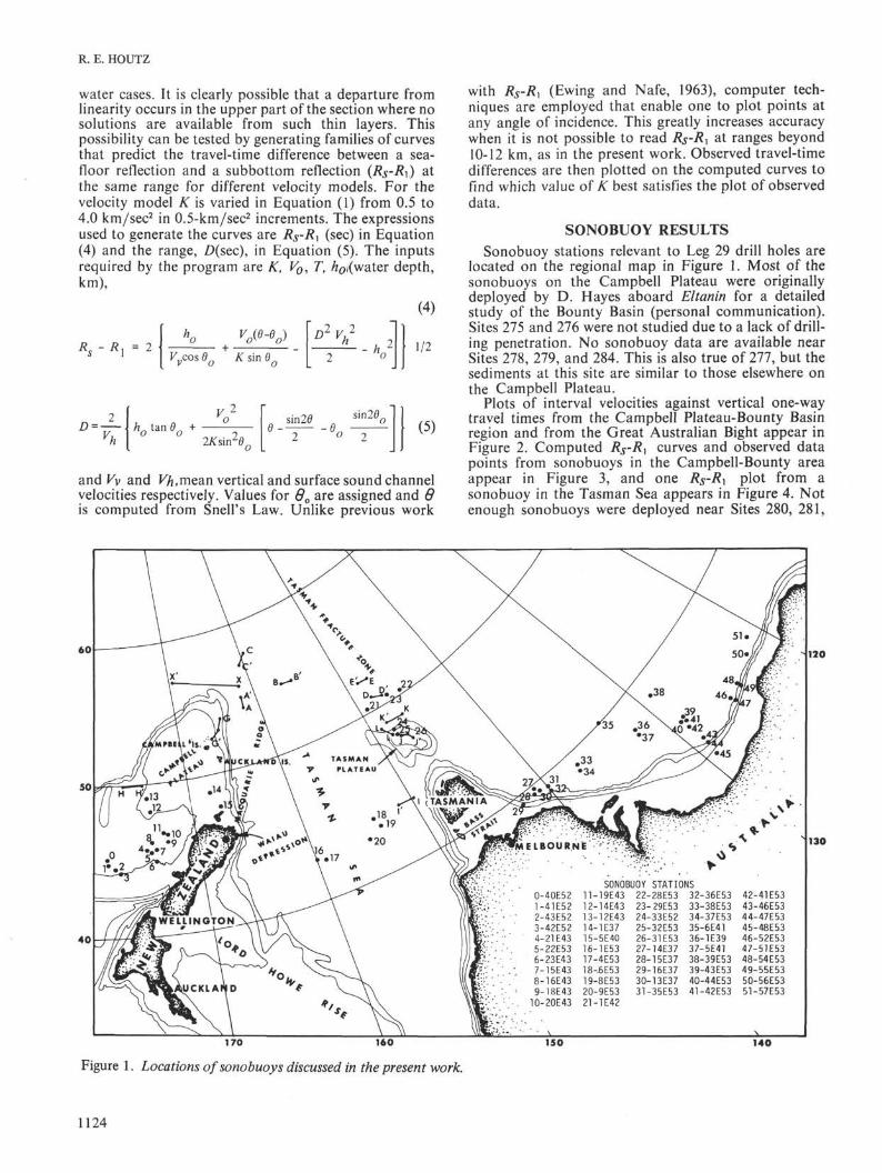
SONOBUOY RESULTSSonobuoy stations relevant to Leg 29 drill holes are

located on the regional map in Figure 1. Most of thesonobuoys on the Campbell Plateau were originallydeployed by D. Hayes aboard Eltanin for a detailedstudy of the Bounty Basin (personal communication).Sites 275 and 276 were not studied due to a lack of drill-ing penetration. No sonobuoy data are available nearSites 278, 279, and 284. This is also true of 277, but thesediments at this site are similar to those elsewhere onthe Campbell Plateau.

Plots of interval velocities against vertical one-waytravel times from the Campbell Plateau-Bounty Basinregion and from the Great Australian Bight appear inFigure 2. Computed Rs-R curves and observed datapoints from sonobuoys in the Campbell-Bounty areaappear in Figure 3, and one Rs-R plot from asonobuoy in the Tasman Sea appears in Figure 4. Notenough sonobuoys were deployed near Sites 280, 281,

SONOBUOY STATIONS11-19E43 22-28E53 32-36E53

23-29E5324-33E5225-32E5326-31E5327-14E3728-15E3729-16E3730-13E3731-35E53

42-41E5343-46E5344-47E5345-48E5346-52E5347-51E5348-54E5349-55E5350-56E5351-57E53

0-40E521-41E522-43E523-42E524-21 E435-22E536-23E437-15E438-16E439-18E4310-20E43

12-14E4313-12E4314-1E3715-5E4016-1E5317-4E5318-.6E5319-8E5320-9E5321-1E42

33-38E5334-37E5335-6E4136-1E3937-5E4138-39E5339-43E5340-44E5341-42E53

120

130

170 160

Figure 1. Locations of sonobuoys discussed in the present work.

150 1 4 0

1124

COMPARISON OF SONOBUOY AND SONIC PROBE MEASUREMENTS WITH DRILLING RESULTS

4.5

4.0

3.5

3.0

2.5

1.5

4.0

3.5

3.0

GREAT AUSTRALIAN BIGHT

V=l.61 + 2.16T + 0.23 km/sec

CAMPBELL-BOUNTY

V=1.55 + 2.47T+0.16 km/sec

0.5sec

1.0

Figure 2. Regressions of interval velocities fromsonobuoy solutions on one-way, vertical travel-time. Standard deviations of each solution arescaled as vertical lines. The regression coefficientsare shown.

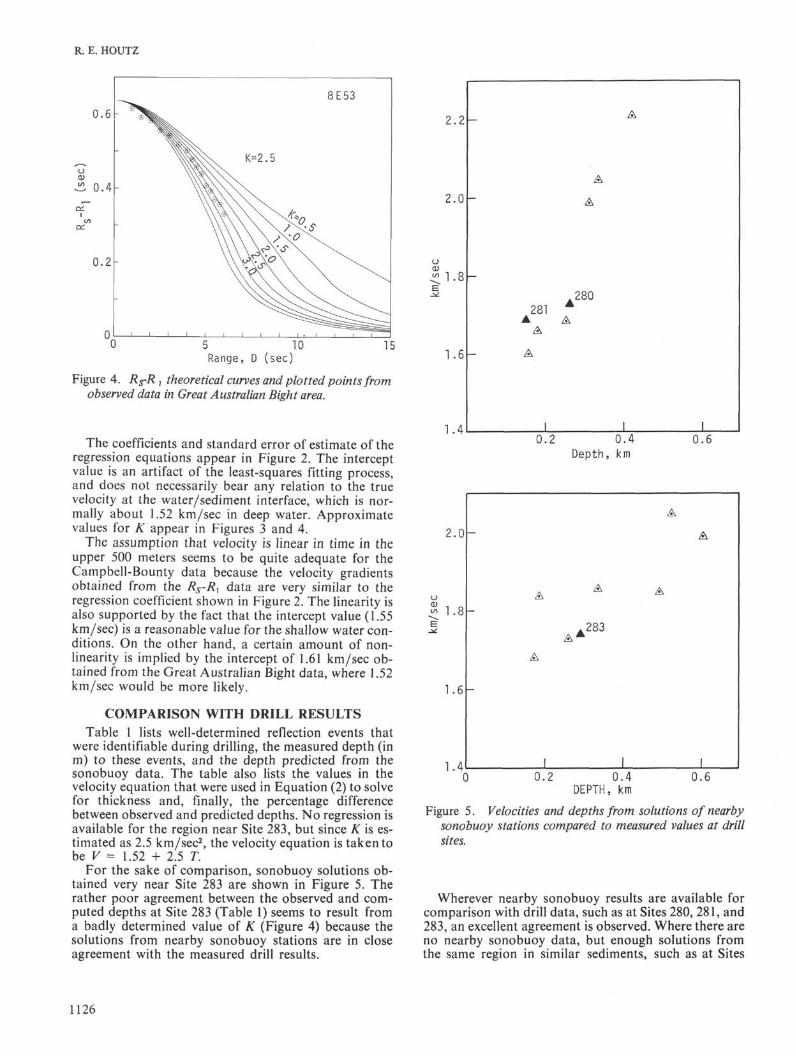
and 283 to make regressional studies. However, the datafrom several sonobuoy solutions from nearby stationsare plotted in Figure 5, so that the observed meanvelocities from the drilling results can be compared withthe sonobuoy data (at the appropriate depths), as shownin the figure. It is apparent that the observed values arenot significantly different from the groupings of com-puted values.

5 n n , . 1 0Range, D (sec)

Figure 3. Rs-R1 theoretical curves and plotted points fromobserved data in Campbell Plateau-Bounty Basin area.

1125

R. E. HOUTZ

0.6

8E53

K=2.5

5 10Range, D (sec)

15

Figure 4. Rs-R , theoretical curves and plotted points fromobserved data in Great Australian Bight area.

The coefficients and standard error of estimate of theregression equations appear in Figure 2. The interceptvalue is an artifact of the least-squares fitting process,and does not necessarily bear any relation to the truevelocity at the water/sediment interface, which is nor-mally about 1.52 km/sec in deep water. Approximatevalues for K appear in Figures 3 and 4.

The assumption that velocity is linear in time in theupper 500 meters seems to be quite adequate for theCampbell-Bounty data because the velocity gradientsobtained from the Rs-R data are very similar to theregression coefficient shown in Figure 2. The linearity isalso supported by the fact that the intercept value (1.55km/sec) is a reasonable value for the shallow water con-ditions. On the other hand, a certain amount of non-linearity is implied by the intercept of 1.61 km/sec ob-tained from the Great Australian Bight data, where 1.52km/sec would be more likely.

COMPARISON WITH DRILL RESULTS

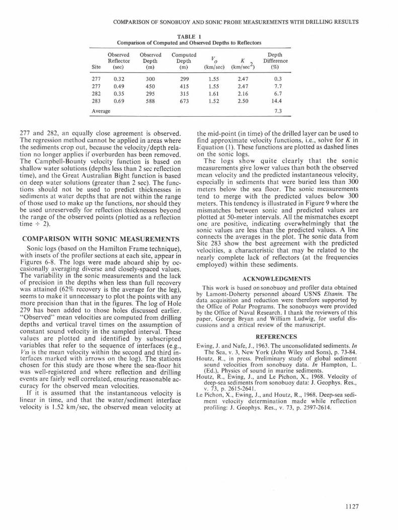
Table 1 lists well-determined reflection events thatwere identifiable during drilling, the measured depth (inm) to these events, and the depth predicted from thesonobuoy data. The table also lists the values in thevelocity equation that were used in Equation (2) to solvefor thickness and, finally, the percentage differencebetween observed and predicted depths. No regression isavailable for the region near Site 283, but since K is es-timated as 2.5 km/sec2, the velocity equation is taken tobe V = 1.52 + 2.5 T.

For the sake of comparison, sonobuoy solutions ob-tained very near Site 283 are shown in Figure 5. Therather poor agreement between the observed and com-puted depths at Site 283 (Table 1) seems to result froma badly determined value of K (Figure 4) because thesolutions from nearby sonobuoy stations are in closeagreement with the measured drill results.

2 . 2 -

0.2 0.4

Depth, km

0.6

2 . 0 -

1 . 8 -

1 . 6 -

1.4

—

A

A

1

A

.283A A

_L

A

A

Δ

10 0.2 0.4

DEPTH, km0.6

Figure 5. Velocities and depths from solutions of nearbysonobuoy stations compared to measured values at drillsites.

Wherever nearby sonobuoy results are available forcomparison with drill data, such as at Sites 280, 281, and283, an excellent agreement is observed. Where there areno nearby sonobuoy data, but enough solutions fromthe same region in similar sediments, such as at Sites

1126

COMPARISON OF SONOBUOY AND SONIC PROBE MEASUREMENTS WITH DRILLING RESULTS

TABLE 1Comparison of Computed and Observed Depths to Reflectors

Site

277277282283

ObservedReflector

(sec)

0.320.490.350.69

Average

ObservedDepth

(m)

300

450295588

ComputedDepth

(m)

299415315673

Vo(km/sec)

1.551.551.611.52

K 2(km/sec )

2.472.472.162.50

DepthDifference

(%)

0.37.7

6.714.4

7.3

277 and 282, an equally close agreement is observed.The regression method cannot be applied in areas wherethe sediments crop out, because the velocity/depth rela-tion no longer applies if overburden has been removed.The Campbell-Bounty velocity function is based onshallow water solutions (depths less than 2 sec reflectiontime), and the Great Australian Bight function is basedon deep water solutions (greater than 2 sec). The func-tions should not be used to predict thicknesses insediments at water depths that are not within the rangeof those used to make up the functions, nor should theybe used unreservedly for reflection thicknesses beyondthe range of the observed points (plotted as a reflectiontime ÷ 2).

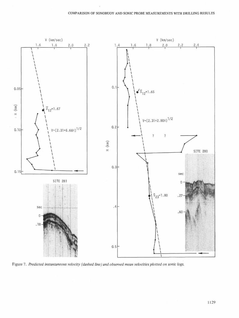
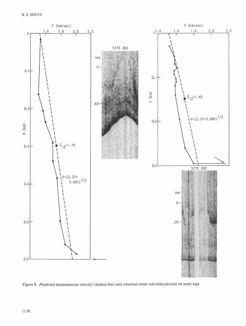
COMPARISON WITH SONIC MEASUREMENTSSonic logs (based on the Hamilton Frame technique),

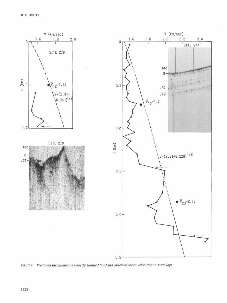
with insets of the profiler sections at each site, appear inFigures 6-8. The logs were made aboard ship by oc-casionally averaging diverse and closely-spaced values.The variability in the sonic measurements and the lackof precision in the depths when less than full recoverywas attained (62% recovery is the average for the leg),seems to make it unnecessary to plot the points with anymore precision than that in the figures. The log of Hole279 has been added to those holes discussed earlier."Observed" mean velocities are computed from drillingdepths and vertical travel times on the assumption ofconstant sound velocity in the sampled interval. Thesevalues are plotted and identified by subscriptedvariables that refer to the sequence of interfaces (e.g.,V22 is the mean velocity within the second and third in-terfaces marked with arrows on the log). The stationschosen for this study are those where the sea-floor hitwas well-registered and where reflection and drillingevents are fairly well correlated, ensuring reasonable ac-curacy for the observed mean velocities.

If it is assumed that the instantaneous velocity islinear in time, and that the water/sediment interfacevelocity is 1.52 km/sec, the observed mean velocity at

the mid-point (in time) of the drilled layer can be used tofind approximate velocity functions, i.e., solve for K inEquation (1). These functions are plotted as dashed lineson the sonic logs.

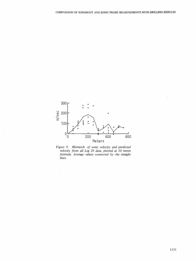
The logs show quite clearly that the sonicmeasurements give lower values than both the observedmean velocity and the predicted instantaneous velocity,especially in sediments that were buried less than 300meters below the sea floor. The sonic measurementstend to merge with the predicted values below 300meters. This tendency is illustrated in Figure 9 where themismatches between sonic and predicted values areplotted at 50-meter intervals. All the mismatches exceptone are positive, indicating overwhelmingly that thesonic values are less than the predicted values. A lineconnects the averages in the plot. The sonic data fromSite 283 show the best agreement with the predictedvelocities, a characteristic that may be related to thenearly complete lack of reflectors (at the frequenciesemployed) within these sediments.

ACKNOWLEDGMENTS

This work is based onsonobuoy and profiler data obtainedby Lamont-Doherty personnel aboard USNS Eltanin. Thedata acquisition and reduction were therefore supported bythe Office of Polar Programs. The sonobuoys were providedby the Office of Naval Research. I thank the reviewers of thispaper, George Bryan and William Ludwig, for useful dis-cussions and a critical review of the manuscript.

REFERENCES

Ewing, J. and Nafe, J., 1963. The unconsolidated sediments. InThe Sea, v. 3, New York (John Wiley and Sons), p. 73-84.

Houtz, R., in press. Preliminary study of global sedimentsound velocities from sonobuoy data. In Hampton, L.(Ed.), Physics of sound in marine sediments.

Houtz, R., Ewing, J., and Le Pichon, X., 1968. Velocity ofdeep-sea sediments from sonobuoy data: J. Geophys. Res.,v. 73, p. 2615-2641.

Le Pichon, X., Ewing, J., and Houtz, R., 1968. Deep-sea sedi-ment velocity determination made while reflectionprofiling: J. Geophys. Res., v. 73, p. 2597-2614.

1127

R. E. HOUTZ

V (km/sec]1.6 1.8 2.0

secSITE 279

-

1.6V (km/sec)2.0 2.2 2.4

SITE 277

0.3

0.4

0.5

s. •*

.

Figure 6. Predicted instantaneous velocity (dashed line) and observed mean velocities on sonic logs.

1128

COMPARISON OF SONOBUOY AND SONIC PROBE MEASUREMENTS WITH DRILLING RESULTS

0.05-

0.10-

0.15-

V (km/sec)

2.2 1.4

SITE 281

0.1

0.2

0.3

.4

0.5

V (km/sec)

2.0 2.2—r~

2.4

V=(2.31+2.80H)1/2

SITE 280

sec

Figure 7. Predicted instantaneous velocity (dashed line) and observed mean velocities plotted on sonic logs.

1129

R. E. HOUTZ

V (km/sec)

1.6 1.8 2.0 2.2 ,1.4

V (km/sec)

1.8 2.2

SITE 282

sec

, 3 5 - ;

Figure 8. Predicted instantaneous velocity (dashed line) and observed mean velocities plotted on sonic logs.

1130

COMPARISON OF SONOBUOY AND SONIC PROBE MEASUREMENTS WITH DRILLING RESULTS

200 400Meters

600

Figure 9. Mismatch of sonic velocity and predictedvelocity from all Leg 29 data, plotted at 50 meterintervals. Average values connected by the straightlines.

1131