Embed Size (px)
Citation preview
1
Wireless Sensor Networks - Node Localization for Various Industry Problems
Kurt Derr, Member, IEEE, Milos Manic, Senior Member, IEEE
Abstract – Fast, effective monitoring following airborne releases of toxic substances is critical to mitigate risks to threatened population areas. Electrically powered systems in industrial settings require monitoring of emitted electromagnetic fields to determine the status of the equipment and ensure their safe operation. In situations such as these, wireless sensor nodes at fixed predetermined locations provide monitoring to ensure safety. A challenging algorithmic problem is determining the locations to place these sensor nodes while meeting several criteria: 1) provide complete coverage of the domain, and 2) create a topology with problem dependent node densities, while 3) minimizing the number of sensor nodes. This manuscript presents a novel approach, Advancing Front mEsh generation with Constrained dElaunay Triangulation and Smoothing (AFECETS) that addresses these criteria. A unique aspect of AFECETS is the ability to determine wireless sensor node locations for areas of high interest (hospitals, schools, high population density areas) that require higher density of nodes for monitoring environmental conditions, a feature that is difficult to find in other research work. The AFECETS algorithm was tested on several arbitrary shaped domains. AFECETS simulation results show that the algorithm 1) provides significant reduction in the number of nodes, in some cases over 40%, compared to an advancing front mesh generation algorithm, 2) maintains and improves optimal spacing between nodes, and 3) produces simulation run times suitable for real-time applications. Index Terms— Wireless sensor network, sensor node, Delaunay triangulation, mesh generation, mesh network, topology.
I. INTRODUCTION Classification of wireless sensor networks (WSNs) may be
based on their application objectives, traffic characteristics, and data delivery requirements. WSN classification/categorization is a significant area of study. A complete survey of classification, or categorization, techniques may be found in [1]-[4].
Typical approaches for WSN classification/categorization are centralized versus distributed [5]-[8], deterministic versus non-deterministic, or single tier versus two tier networks [9]-[12]. Distributed algorithms are an optimal selection when Manuscript received March 7, 2014. Accepted for publication January 6, 2015. Copyright © 2009 IEEE. Personal use of this material is permitted. However, permission to use this material for any other purposes must be obtained from the IEEE by sending a request to [email protected]. Kurt Derr is with the Idaho National Laboratory, Idaho Falls, ID 83415 USA (e-mail: [email protected], or [email protected]). Milos Manic is with Virginia Commonwealth University, Richmond, Va. 23284 USA (e-mail: [email protected]).
mobile nodes are an option and complete domain information is not available. Centralized algorithms are an appropriate choice for determining sensor positions when the geometry of the domain is known a priori and the domain does not support the use of mobile sensor nodes, such as within a metropolitan area. Centralized algorithms are able to create a topology that is an optimum outcome due to a global view of the domain.
A prime application of Wireless Sensor Networks (WSNs) is collecting sensory data from phenomenon and delivering that data to users through base stations located outside of the monitored domain. The sensors may form a mesh network where each sensor may capture, disseminate, and relay data. Several key aspects of the sensor node deployment are 1) selecting the best sensor locations for monitoring of the domain [13], 2) the ability of the deployed network to provide complete communication [14] and sensing coverage [15] of the domain, and 3) a sensor topology with appropriate node densities in different areas of the domain.
This manuscript presents a novel mesh creation algorithm, AFECETS, which generates a mesh using the Advancing Front Mesh generation (AFMG) algorithm with Constrained Delaunay triangulation, smoothing, and heuristics to create an optimal topology. AFMG was chosen since the algorithm is a robust and reliable mesh generation technique for producing meshes in complex geometries. AFECETS creates a sensor node topology for convex and non-convex polygonal domains requiring multiple areas of varying sensor density while minimizing the number of nodes in the network.
The rest of the manuscript is organized as follows: Section II discusses related work; Section III provides a detailed formulation of the problem being solved and preliminaries; Section IV discusses constrained Delaunay triangulation and smoothing; Section V discusses the AFECETS simulation test results; Section VI presents industrial environments for AFECETS; and Section VII presents our conclusions.
II. RELATED WORK
Szczytowski [16] addresses the sensing problem of a phenomena gradually changing over a monitored area. A distributed adaptive sampling technique, ASample, is presented which detects both under and over sampled regions. ASample presumes an arbitrary spatial distribution of sensor nodes that fully covers the domain. However, an arbitrary spatial distribution of static (non mobile) nodes will not typically result in an optimal deployment. The strength of the ASample algorithm is the use of mobile nodes to optimize the deployment. This differs from the goal of the AFECETS
2
algorithm, which is to calculate the positions for static sensor nodes that result in an optimal deployment.
Qu [17] assumes that mobile sensors are initially randomly deployed in some domain, whereas AFECETS utilizes static sensors nodes. A centralized relocating algorithm is introduced to minimize sensor movement and prolong the lifetime of the sensor network. The centralized algorithm uses Particle Swarm Optimization to minimize movement and save energy, and Voronoi diagrams to ensure that sensors cover the entire sensing domain. However, unlike AFECETS, this algorithm will not produce uniform distributions of nodes in multiple areas of the domain.
Wang [18] presents a centralized approach to determining the locations of sensors in an arbitrary shaped region by partitioning the sensing field into smaller sub fields based on the shape of the field. The partitioning algorithms are not thoroughly described. This centralized approach does not produce uniform distributions of nodes in multiple areas of the domain like AFECETS.
Mesh generation techniques [19], such as the Advancing Front Mesh Generation algorithm, are used in both finite element analysis and computational fluid dynamics. These algorithms tend to create nodes as necessary to discretize the domain and conform to the boundary, resulting in a non-uniform distribution of nodes. This differs from the goal of the AFECETS algorithm, which is to produce a uniform distribution of nodes in multiple areas of the domain.
Schwager [20] presents a distributed approach for robots to spread out over an environment and provide adaptive sensing coverage. The robots use an online learning system to determine the areas that require higher density sensing coverage while exploring the environment using a traveling salesman (TSP) based method. A weighting function represents the importance of the different areas of the environment. This distributed approach assumes that the sensing nodes are mobile, whereas AFECETS assumes static nodes for appropriate problem distributions.
Poe [21] investigates random and deterministic node deployments algorithms for large-scale wireless sensor networks. The performances of the WSNs are analyzed based on coverage, energy consumption, and message transfer delay. Simple convex deployment areas are selected to demonstrate the effectiveness of this algorithm, whereas the AFECETS algorithm provides near optimal sensor node deployment in both convex and non-convex domains.
The AFECETS algorithm differs from the approaches described above in that the AFECETS nodes are static, the algorithm works in both convex and non-convex polygonal domains, and the algorithm produces a uniform distribution of nodes in multiple areas of the domain.
III. PROBLEM FORMULATION AND PRELIMINARIES
A WSN is used to monitor and measure a varying distribution of contaminants (non-uniform phenomena distribution) in a bounded domain [22]-[24] using a centralized algorithm approach. We are given a set of sensors or nodes, V=v1,v2,…,vn, sufficient to provide complete coverage of a
domain, where every sensor, or node, in V has a sensing and communications range sufficient to satisfy the desired internodal spacing [25]-[26]. The desired internodal spacing may vary in different areas of a domain based on the sensing and communications requirements. The nodes consist of both boundary nodes, VB, and internal nodes VI. The nodes are NOT mobile and require manual placement.
A scenario for the use of a centralized algorithm for determining the locations of sensor nodes is as follows. A number of cities around the world suffer from major air pollution. These domains represent metropolitan areas and their surrounding suburbs where the density of people varies throughout the domain. The concentration of contaminants varies in each domain due to varying numbers of motor vehicles, factories, and other contaminant sources. Population statistics are available and city governments need to determine where to place sensor nodes to monitor contaminants to evaluate the danger to the public and provide appropriate warnings. Direct correlations exist between population density and atmospheric pollutants. The AFECETS algorithm will be used to determine the location for sensor nodes based on node densities for specific areas, correlated to population densities, provided by the city governments.
Additionally, a city may also require sensor nodes to be placed in high interest areas in the event of a disaster as illustrated in a SIM Center US-Ignite video [27]. A city would likely have both high and low interest areas based on areas of high population densities, and buildings serving the public such as hospitals, schools, and government facilities. The AFECETS algorithm would be effective in determining the locations to place sensor nodes in these instances as well.
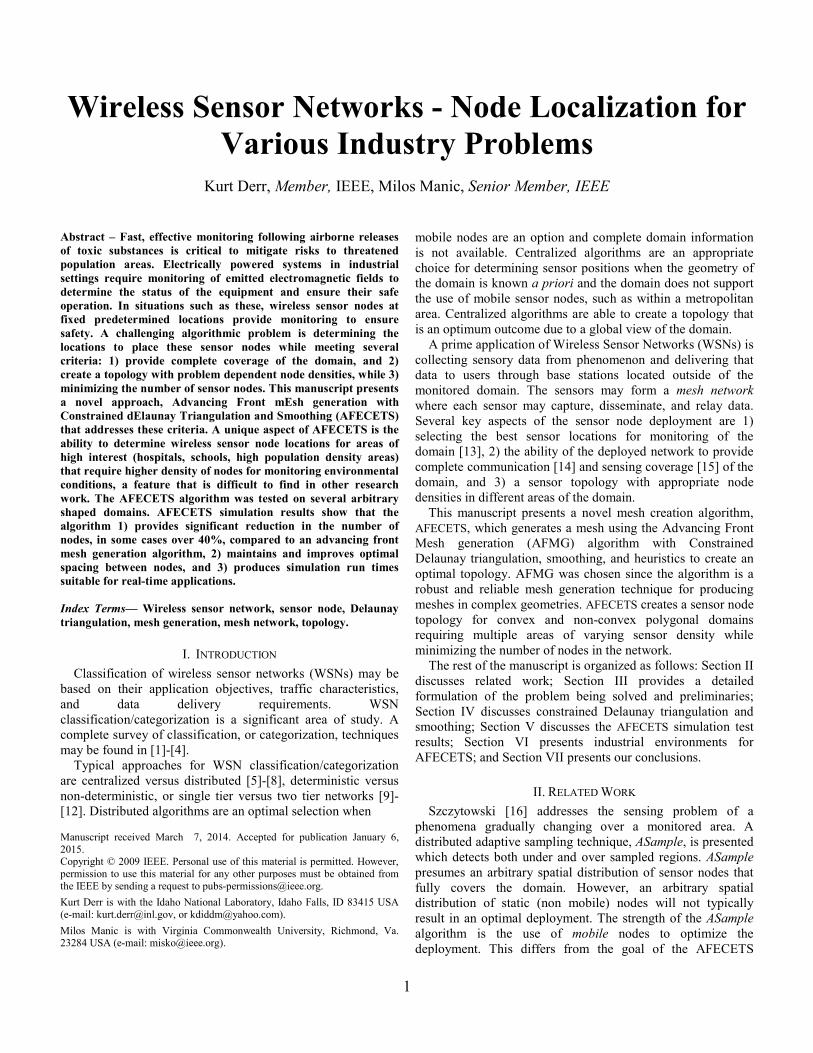
Fig. 1 shows two bounded domains with different shapes representing metropolitan areas that will be used to demonstrate the effectiveness of the AFECETS algorithm. Each domain has an area of High sensory Interest (HI), represented as a circle, where high population densities will create high concentrations of pollutants and areas of Low sensory Interest (LI) where lower population densities produce fewer pollutants.
The circular HI areas of Fig. 1 represent dense population areas where the concentration of sensor nodes must be greater than the LI areas to acquire granular contaminant measurement data. The challenge is to create a mesh topology that meets the following requirements:
1. Maintains complete sensing and communications coverage of the domain while minimizing the cost (number of sensors),
2. Determines the locations for sensor nodes in the HI area where the population is dense and sensor nodes are closely spaced,
3. Determines the locations for sensor nodes in the LI area where the population is sparse and the spacing between nodes is greater than in the HI area,
4. Forms an equilateral triangular mesh with the mesh in the HI area connecting with the mesh in the LI area, and
3
5. The sensor topology maintains multiple communications paths between neighboring sensors to maximize the robustness of the network.
a) Domain 1
a) Domain 2
Fig. 1. Bounded Domains with Circular Areas of High Sensory Interest The terms and notation used in this manuscript are defined in Table I. Parameter default values are noted in parenthesis.
TABLE I SENSOR MESH NETWORK MAJOR TERMS AND NOTATION
Term Definition WSN Wireless Sensor Network HI High Sensory Interest LI Low Sensory Interest CDT Constrained Delaunay Triangulation VB Boundary nodes VI Internal nodes q Triangle quality metric FE Formation Effectiveness E Energy of the mesh |ViVj| Distance between sensors i and j AEL Average Edge Length ATS Average Triangle Size
A Polygonal area cx,cy Centroid coordinates of a polygon d Distance from node to polygon centroid Ω Domain of the mesh ∂Ω Boundary of a domain δ Desired spacing between nodes; δHI in HI area (20
meters), δLI in LI area (40 meters) λ Movement threshold #∆ Number of triangles (density metric) # Nodes Number of nodes (density metric)
The term nodes will be used to refer to sensor nodes (SNs)
throughout this manuscript. The problem of optimal placement of nodes in a sensor network necessary to completely cover the entire monitoring area was proven to be NP-complete [28] for most formulations of WSN deployments. Additionally, given L possible locations for nodes and N nodes, there are LN possible mesh sensor networks. The goal of the algorithmic approach in this manuscript is to determine an optimal solution providing, 1) complete coverage and 2) maximum formation, while minimizing the number of nodes and achieving specific internodal spacing. Optimality is affected by geographic constraints such as the boundary, obstacles, and shape of the deployment area [29]-[32].
A. Mesh Generation Metrics
Several metrics will be used to evaluate the performance of the centralized mesh generation, or sensor node configuration, algorithms. These metrics are explained in detail in [19] and are briefly summarized here.
The metrics that will be used to evaluate the quality of the generated mesh are average edge length (AEL), average triangle size (ATS), triangle quality q, number of nodes, formation effectiveness, and mesh energy (E). AEL (Average Edge Length) is the average edge length between nodes in the network. δ is the desired edge length between network nodes. δHI represents the desired edge length between nodes in the HI area and δLI represents the desired edge length between nodes in the LI area. ATS (Average Triangle Size) is the average triangle size in the generated mesh. The ideal equilateral triangle size (ITS) with 40 and 20 meter spacing between nodes is 692.8 and 173.2 square meters, respectively. The ideal equilateral triangle size is computed as:
432bS =
where b is the length of a side of the triangle and S is the size of the triangle in square meters. Triangle Quality (q) is the triangle quality metric [33], q, defined as:
23
22
21
34hhh
aq++
= (1)
where a is the area of the triangle; h1, h2, h3 are the lengths of triangle sides. A triangle is equilateral, the ideal case, when q equals 1. Number of Nodes is the number of nodes in both the HI and LI areas.
4
Formation Effectiveness [34], FE, is a measure of the ideal spacing arrangement between nodes in a domain.
In
AF
ni i
E *1∑ == , 10 ≤< EF (2)
where Ai is the size of triangle i in the mesh, I is the ideal triangle size (ITS), and n is the number of triangles in mesh. Mesh Energy (E) is a measure of the energy of the mesh. The entire graph G(V, E) of the sensor network, where V represents the nodes/sensors and E represents the edges/connections between the nodes, can be modeled as a mass spring mesh. The optimal distance between the nodes is the desired edge length, or rest length of each spring. Each node represents a point mass. The total energy of the mesh is [33]-[35]:
2
1)(
21
ijjiijn
i NjdppkE
i
−−∑ ∑== ∈
(3)
21
ijij d
k = (4)
where pi and pj are the coordinates of two connected nodes, dij is the desired edge length between nodes i and j, kij is a spring constant for the spring connecting nodes i and j, Ni represents the nodes adjacent to node i, and n is the number of nodes in the network.
The spring mass damper system, or mesh network, reaches the optimal state when E in (3) is minimized. If the distance between all nodes is equal to the rest length, then the energy of the mesh is zero. However, an equilibrium state in which the mesh energy is zero is generally not achievable given a specific desired edge length between nodes, a goal of minimizing the number of nodes, and the geographic constraints of boundaries, obstacles, and shape of the monitored domain. Therefore, the goal of the AFECETS algorithm is to determine a set of node positions that minimizes the mesh energy.
B. Advanced Front Mesh Generation Algorithm
The AFECETS algorithm has two fundamental parts, the 1) AFMG algorithm and 2) the CETS algorithm. AFMG is a time-honored algorithm for the discretization of a domain. The boundary of the domain, a desired edge length, and the desired number of nodes are user specified configuration parameters to the AFECETS algorithm.
The AFMG algorithm was chosen over other spatial decomposition methods because AFMG gives the mesh maximum flexibility to address complex geometries, such as in Fig. 3, as well as to control mesh point distribution. AFMG produces a higher quality mesh than other spatial decomposition methods by constructing the mesh an element at a time, iteratively selecting optimal points to create mesh elements. The AFMG algorithm starts from an initial front, the boundary of the domain, and constructs the mesh element by element sweeping a front across the domain creating triangular surfaces. The details of the AFMG algorithm can be found in [19].
The problem of finding the discretization of a domain is known as mesh generation. A triangulation of the closed bounded domain, Ω, is referred to as a mesh of Ω. The
connectivity of the mesh is the connection between the vertices, where V represents a set of nodes and E the set of edges, or connections, between those nodes.
AFMG Generated Meshes
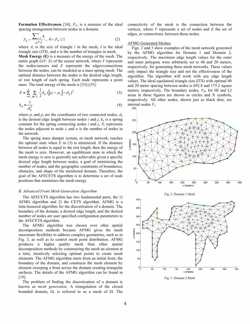
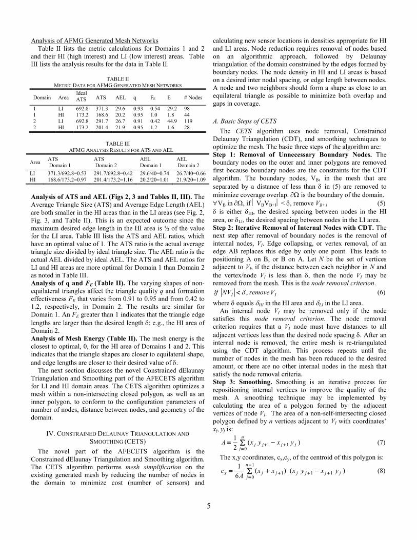
Figs. 2 and 3 show examples of the mesh network generated by the AFMG algorithm for Domain 1 and Domain 2, respectively. The maximum edge length values for the outer and inner polygons were arbitrarily set to 40 and 20 meters, respectively, for generating these mesh networks. These values only impact the triangle size and not the effectiveness of the algorithm. The algorithm will work with any edge length values. The ideal equilateral triangle size (ITS) with optimal 40 and 20 meter spacing between nodes is 692.8 and 173.2 square meters, respectively. The boundary nodes, VB, for HI and LI areas in these figures are shown as circles and X symbols, respectively. All other nodes, shown just as black dots, are internal nodes VI.
Fig. 2. Domain 1 Mesh
Fig. 3. Domain 2 Mesh
5
Analysis of AFMG Generated Mesh Networks Table II lists the metric calculations for Domains 1 and 2
and their HI (high interest) and LI (low interest) areas. Table III lists the analysis results for the data in Table II.
TABLE II
METRIC DATA FOR AFMG GENERATED MESH NETWORKS
Domain Area Ideal ATS ATS AEL q FE E # Nodes
1 LI 692.8 371.3 29.6 0.93 0.54 29.2 98 1 HI 173.2 168.6 20.2 0.95 1.0 1.8 44 2 LI 692.8 291.7 26.7 0.91 0.42 44.9 119 2 HI 173.2 201.4 21.9 0.95 1.2 1.6 28
TABLE III AFMG ANALYSIS RESULTS FOR ATS AND AEL
Area ATS Domain 1
ATS Domain 2
AEL Domain 1
AEL Domain 2
LI 371.3/692.8=0.53 291.7/692.8=0.42 29.6/40=0.74 26.7/40=0.66 HI 168.6/173.2=0.97 201.4/173.2=1.16 20.2/20=1.01 21.9/20=1.09 Analysis of ATS and AEL (Figs 2, 3 and Tables II, III). The Average Triangle Size (ATS) and Average Edge Length (AEL) are both smaller in the HI areas than in the LI areas (see Fig. 2, Fig. 3, and Table II). This is an expected outcome since the maximum desired edge length in the HI area is ½ of the value for the LI area. Table III lists the ATS and AEL ratios, which have an optimal value of 1. The ATS ratio is the actual average triangle size divided by ideal triangle size. The AEL ratio is the actual AEL divided by ideal AEL. The ATS and AEL ratios for LI and HI areas are more optimal for Domain 1 than Domain 2 as noted in Table III. Analysis of q and FE (Table II). The varying shapes of non-equilateral triangles affect the triangle quality q and formation effectiveness FE that varies from 0.91 to 0.95 and from 0.42 to 1.2, respectively, in Domain 2. The results are similar for Domain 1. An FE greater than 1 indicates that the triangle edge lengths are larger than the desired length δ; e.g., the HI area of Domain 2. Analysis of Mesh Energy (Table II). The mesh energy is the closest to optimal, 0, for the HI area of Domains 1 and 2. This indicates that the triangle shapes are closer to equilateral shape, and edge lengths are closer to their desired value of δ.
The next section discusses the novel Constrained dElaunay Triangulation and Smoothing part of the AFECETS algorithm for LI and HI domain areas. The CETS algorithm optimizes a mesh within a non-intersecting closed polygon, as well as an inner polygon, to conform to the configuration parameters of number of nodes, distance between nodes, and geometry of the domain.
IV. CONSTRAINED DELAUNAY TRIANGULATION AND SMOOTHING (CETS)
The novel part of the AFECETS algorithm is the Constrained dElaunay Triangulation and Smoothing algorithm. The CETS algorithm performs mesh simplification on the existing generated mesh by reducing the number of nodes in the domain to minimize cost (number of sensors) and
calculating new sensor locations in densities appropriate for HI and LI areas. Node reduction requires removal of nodes based on an algorithmic approach, followed by Delaunay triangulation of the domain constrained by the edges formed by boundary nodes. The node density in HI and LI areas is based on a desired inter nodal spacing, or edge length between nodes. A node and two neighbors should form a shape as close to an equilateral triangle as possible to minimize both overlap and gaps in coverage.
A. Basic Steps of CETS
The CETS algorithm uses node removal, Constrained Delaunay Triangulation (CDT), and smoothing techniques to optimize the mesh. The basic three steps of the algorithm are: Step 1: Removal of Unnecessary Boundary Nodes. The boundary nodes on the outer and inner polygons are removed first because boundary nodes are the constraints for the CDT algorithm. The boundary nodes, VB, in the mesh that are separated by a distance of less than δ in (5) are removed to minimize coverage overlap. ∂Ω is the boundary of the domain. ∀VB in ∂Ω, if VBVB+1< δ, remove VB+1 (5) δ is either δHI, the desired spacing between nodes in the HI area, or δLI, the desired spacing between nodes in the LI area. Step 2: Iterative Removal of Internal Nodes with CDT. The next step after removal of boundary nodes is the removal of internal nodes, VI. Edge collapsing, or vertex removal, of an edge AB replaces this edge by only one point. This leads to positioning A on B, or B on A. Let N be the set of vertices adjacent to VI, if the distance between each neighbor in N and the vertex/node VI is less than δ, then the node VI may be removed from the mesh. This is the node removal criterion.
II VremoveNVif ,δ< (6) where δ equals δHI in the HI area and δLI in the LI area.
An internal node VI may be removed only if the node satisfies this node removal criterion. The node removal criterion requires that a VI node must have distances to all adjacent vertices less than the desired node spacing δ. After an internal node is removed, the entire mesh is re-triangulated using the CDT algorithm. This process repeats until the number of nodes in the mesh has been reduced to the desired amount, or there are no other internal nodes in the mesh that satisfy the node removal criteria. Step 3: Smoothing. Smoothing is an iterative process for repositioning internal vertices to improve the quality of the mesh. A smoothing technique may be implemented by calculating the area of a polygon formed by the adjacent vertices of node VI. The area of a non-self-intersecting closed polygon defined by n vertices adjacent to VI with coordinates’ xj, yj is:
∑ −==
++
n
jjjjj yxyxA
011 )(
21 (7)
The x,y coordinates, cx,cy, of the centroid of this polygon is:
∑ −+=−
=+++
1
0111 )()(
61 n
jjjjjjjx yxyxxx
Ac (8)
6
∑ −+=−
=+++
1
0111 )()(
61 n
jjjjjjjy yxyxyy
Ac (9)
The smoothing algorithm is described by: λ>⇔∀ dcctovmoveccAcalculatevvwithV yxiyxiyxI ;,,
(10) 22 )()( yyxx cvcvd −+−= (11)
The smoothing algorithm in (10) iterates through all of the internal vertices VI of the mesh calculating the polygonal area in (7) of the vertices adjacent to VI, the centroid point of the polygon with (8) and (9), and the distance d in (11) from the node VI to the centroid cx,cy. If d is greater than λ, node VI is moved to cx,cy. The smoothing algorithm terminates when the average internal node movement is less than or equal to the movement threshold λ. Smoothing effectively moves sensor nodes to lower energy positions in the mesh network. B. Pseudo Code for CETS Algorithm
The high-level pseudo code for the CETS algorithm is listed in Table IV.
TABLE IV CETS ALGORITHM FOR OUTER AND INNER POLYGONS
Line # Definition
1 Reduce # of boundary nodes, VB, on polygon boundaries based on desired node spacing
2 LOOP 3 Re-triangulate outer polygon using
Constrained Delaunay Triangulation (CDT) 4 Remove an internal node, VI, in the outer polygon
to achieve δLI desired inter-nodal spacing 5 UNTIL minimum node count reached, or node removal criteria
no longer satisfied 6 Perform Laplacian smoothing on VI nodes in outer polygon 7 LOOP 8 Re-triangulate inner polygon using CDT 9 Remove an internal node, VI, in the inner polygon
to achieve δHI desired node spacing 10 UNTIL minimum node count reached, or node removal criteria
no longer satisfied 11 Perform Laplacian smoothing on VI nodes in inner polygon
The algorithm outlined in Table IV reduces the number of nodes on the polygon boundaries and applies the Constrained Delaunay Triangulation algorithm. Next, the polygonal areas are re-triangulated while removing nodes that meet the node removal criteria. The last step is to perform Laplacian smoothing on all polygonal areas.
The next section discusses the results of applying the CETS algorithm to the AFMG meshes for the domains in Fig. 1.
V. AFECETS SIMULATION TEST RESULTS
This section illustrates the advantages of the AFECETS algorithm over the AFMG algorithm. The simulation results of the AFECETS algorithm are now examined for the HI and LI areas of Fig. 1. These simulations were developed with MATLAB student version 7.8. The desired node spacing, or edge length between nodes, in the HI area and LI areas is arbitrarily selected as 20 (δHI) and 40 (δLI) meters, respectively.
This edge length is chosen based on the desired spacing between nodes.
Multiple areas with different communications and sensing requirements may be optimized by the AFECETS algorithm, rather than just one LI and one HI area. The AFECETS algorithm places no limit on the number of areas within a domain that may have different communications and sensing requirements. The goal is for a node and two neighbors to form a shape as close to an equilateral triangle as possible in both LI and HI areas.
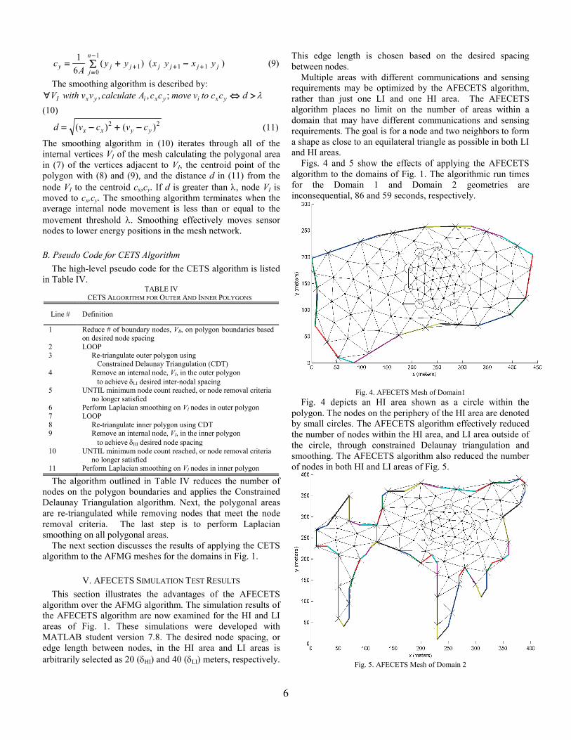
Figs. 4 and 5 show the effects of applying the AFECETS algorithm to the domains of Fig. 1. The algorithmic run times for the Domain 1 and Domain 2 geometries are inconsequential, 86 and 59 seconds, respectively.
Fig. 4. AFECETS Mesh of Domain1 Fig. 4 depicts an HI area shown as a circle within the
polygon. The nodes on the periphery of the HI area are denoted by small circles. The AFECETS algorithm effectively reduced the number of nodes within the HI area, and LI area outside of the circle, through constrained Delaunay triangulation and smoothing. The AFECETS algorithm also reduced the number of nodes in both HI and LI areas of Fig. 5.
Fig. 5. AFECETS Mesh of Domain 2
7
A. Analysis of AFECETS Simulation Results Table V lists the metrics data for the AFECETS algorithm
simulations. This table presents the values of the metrics produced by the AFECETS algorithm for Domains 1 and 2. These metric values may be compared to the values produced by the AFMG algorithm in Table II to demonstration the improvements that the AFECETS provides over the AFMG algorithm; e.g., a reduction in the number of nodes necessary to provide coverage, improvement in triangle quality q, ATS values that are closer to the ideal triangle sizes, and AEL, FE, and E values closer to optimal.
Table VI shows how close the average triangle sizes are to the ideal triangle sizes using the average triangle sizes from Table V. The optimal ratio of average to ideal triangle size is 1. The AFECETS algorithm produced significantly more optimal triangle sizes for LI areas compared to the AFMG algorithm data listed in Table III.
TABLE V AFECETS METRICS DATA
Domain Area Ideal ATS ATS AEL q FE E #
Nodes 1 LI 692.8 603.5 38.7 0.92 0.87 8.6 69 1 HI 173.2 188.9 21.8 0.92 1.1 9.1 34 2 LI 692.8 584.3 39.1 0.88 0.84 10.5 67 2 HI 173.2 235.7 24.6 0.92 1.4 8.2 20
TABLE VI AFECETS ANALYSIS RESULTS FOR ATS AND AEL
Area ATS Domain 1
ATS Domain 2
AEL Domain 1
AEL Domain 2
LI 603.5/692.8=0.87 584.3/692.8=0.84 38.7/40=0.96 39.1/40=0.97 HI 188.9/173.2=1.09 235.7/173.2=1.36 21.8/20=1.09 24.6/20=1.23 Analysis of ATS and AEL (Table VI). Highly irregular shaped polygons like Domain 2 are more difficult to create optimal mesh structures for than more traditional polygons such as in Domain 1. This difficulty is evident in examination of the data in Table V. The ATS for Domain 1 is closer to optimal then for Domain 2 for both LI and HI areas as shown in Table VI. The AEL for Domain 1 of the HI area is closer to optimal than for Domain 2, while the AEL for the LI area of Domains 1 and 2 are virtually the same. Analysis of FE (Table V). The smaller range of FE values for the AFECETS algorithm is due to AEL values being closer to their optimal. The FE values in Table V range from 0.84 to 1.4 (range of 0.56), whereas the FE values in Table II for the AFMG algorithm range from 0.42 to 1.2 (range of 0.78). These results demonstrate that the AFECETS algorithm produces a more optimal configuration that the AFMG algorithm.
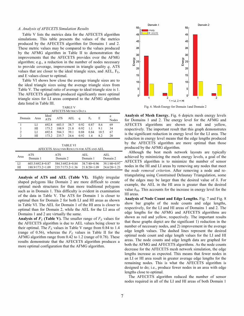
Fig. 6. Mesh Energy for Domain 1and Domain 2
Analysis of Mesh Energy. Fig. 6 depicts mesh energy levels for Domains 1 and 2. The energy level for the AFMG and AFECETS algorithms are shown as red and yellow, respectively. The important result that this graph demonstrates is the significant reduction in energy level for the LI area. The reduction in energy level means that the edge lengths produced by the AFECETS algorithm are more optimal than those produced by the AFMG algorithm.
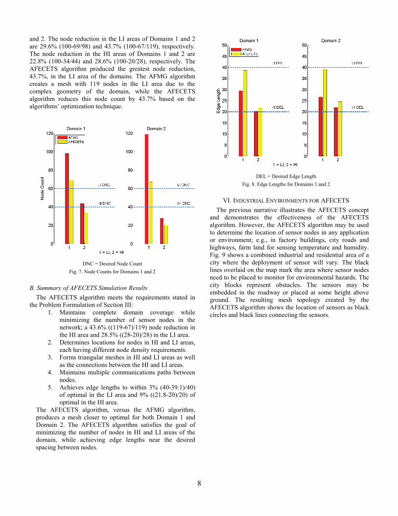
Although the best mesh network layouts are typically achieved by minimizing the mesh energy levels, a goal of the AFECETS algorithm is to minimize the number of sensor nodes in the HI and LI areas by removing any nodes that meet the node removal criterion. After removing a node and re-triangulating using Constrained Delaunay Triangulation, some of the edges may be larger than the desired value of δ. For example, the AEL in the HI area is greater than the desired value δHI. This accounts for the increase in energy level for the HI areas. Analysis of Node Count and Edge Lengths. Fig. 7 and Fig. 8 show bar graphs of the node counts and edge lengths, respectively, for the LI and HI areas of Domains 1 and 2. The edge lengths for the AFMG and AFECETS algorithms are shown as red and yellow, respectively. The important results that these graphs depict are the significant 1) reduction in the number of necessary nodes, and 2) improvement in the average edge length values. The dashed lines represent the desired optimal node count and edge length values for the LI and HI areas. The node counts and edge length data are graphed for both the AFMG and AFECETS algorithms. As the node counts decrease for the AFECETS mesh network simulation, the edge lengths increase as expected. This means that fewer nodes in an LI or HI area result in greater average edge lengths for the remaining nodes. This is what the AFECETS algorithm is designed to do; i.e., produce fewer nodes in an area with edge lengths close to optimal.
The AFECETS algorithm reduced the number of sensor nodes required in all of the LI and HI areas of both Domain 1
8
and 2. The node reduction in the LI areas of Domains 1 and 2 are 29.6% (100-69/98) and 43.7% (100-67/119), respectively. The node reduction in the HI areas of Domains 1 and 2 are 22.8% (100-34/44) and 28.6% (100-20/28), respectively. The AFECETS algorithm produced the greatest node reduction, 43.7%, in the LI area of the domains. The AFMG algorithm creates a mesh with 119 nodes in the LI area due to the complex geometry of the domain, while the AFECETS algorithm reduces this node count by 43.7% based on the algorithms’ optimization technique.
DNC = Desired Node Count
Fig. 7. Node Counts for Domains 1 and 2 B. Summary of AFECETS Simulation Results
The AFECETS algorithm meets the requirements stated in the Problem Formulation of Section III:
1. Maintains complete domain coverage while minimizing the number of sensor nodes in the network; a 43.6% ((119-67)/119) node reduction in the HI area and 28.5% ((28-20)/28) in the LI area.
2. Determines locations for nodes in HI and LI areas, each having different node density requirements.
3. Forms triangular meshes in HI and LI areas as well as the connections between the HI and LI areas.
4. Maintains multiple communications paths between nodes.
5. Achieves edge lengths to within 3% (40-39.1)/40) of optimal in the LI area and 9% ((21.8-20)/20) of optimal in the HI area.
The AFECETS algorithm, versus the AFMG algorithm, produces a mesh closer to optimal for both Domain 1 and Domain 2. The AFECETS algorithm satisfies the goal of minimizing the number of nodes in HI and LI areas of the domain, while achieving edge lengths near the desired spacing between nodes.
DEL = Desired Edge Length
Fig. 8. Edge Lengths for Domains 1 and 2
VI. INDUSTRIAL ENVIRONMENTS FOR AFECETS The previous narrative illustrates the AFECETS concept
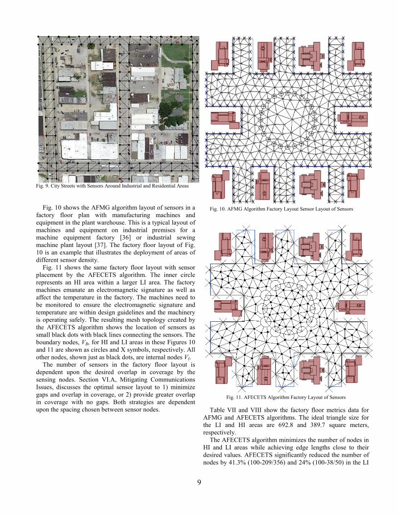
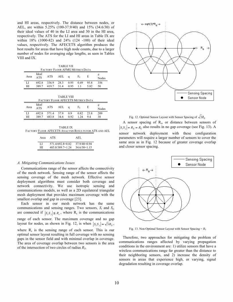
and demonstrates the effectiveness of the AFECETS algorithm. However, the AFECETS algorithm may be used to determine the location of sensor nodes in any application or environment; e.g., in factory buildings, city roads and highways, farm land for sensing temperature and humidity. Fig. 9 shows a combined industrial and residential area of a city where the deployment of sensor will vary. The black lines overlaid on the map mark the area where sensor nodes need to be placed to monitor for environmental hazards. The city blocks represent obstacles. The sensors may be embedded in the roadway or placed at some height above ground. The resulting mesh topology created by the AFECETS algorithm shows the location of sensors as black circles and black lines connecting the sensors.
9
Fig. 9. City Streets with Sensors Around Industrial and Residential Areas
Fig. 10 shows the AFMG algorithm layout of sensors in a factory floor plan with manufacturing machines and equipment in the plant warehouse. This is a typical layout of machines and equipment on industrial premises for a machine equipment factory [36] or industrial sewing machine plant layout [37]. The factory floor layout of Fig. 10 is an example that illustrates the deployment of areas of different sensor density.
Fig. 11 shows the same factory floor layout with sensor placement by the AFECETS algorithm. The inner circle represents an HI area within a larger LI area. The factory machines emanate an electromagnetic signature as well as affect the temperature in the factory. The machines need to be monitored to ensure the electromagnetic signature and temperature are within design guidelines and the machinery is operating safely. The resulting mesh topology created by the AFECETS algorithm shows the location of sensors as small black dots with black lines connecting the sensors. The boundary nodes, VB, for HI and LI areas in these Figures 10 and 11 are shown as circles and X symbols, respectively. All other nodes, shown just as black dots, are internal nodes VI.
The number of sensors in the factory floor layout is dependent upon the desired overlap in coverage by the sensing nodes. Section VI.A, Mitigating Communications Issues, discusses the optimal sensor layout to 1) minimize gaps and overlap in coverage, or 2) provide greater overlap in coverage with no gaps. Both strategies are dependent upon the spacing chosen between sensor nodes.
Fig. 10. AFMG Algorithm Factory Layout Sensor Layout of Sensors
Fig. 11. AFECETS Algorithm Factory Layout of Sensors
Table VII and VIII show the factory floor metrics data for
AFMG and AFECETS algorithms. The ideal triangle size for the LI and HI areas are 692.8 and 389.7 square meters, respectively.
The AFECETS algorithm minimizes the number of nodes in HI and LI areas while achieving edge lengths close to their desired values. AFECETS significantly reduced the number of nodes by 41.3% (100-209/356) and 24% (100-38/50) in the LI
10
and HI areas, respectively. The distance between nodes, or AEL, are within 5.25% (100-37.9/40) and 15% (34.6/30) of their ideal values of 40 in the LI area and 30 in the HI area, respectively. The ATS for the LI and HI areas in Table IX are within 18% (1000-82) and 24% (124 -100) of their ideal values, respectively. The AFECETS algorithm produces the best results for areas that have high node counts, due to a larger number of nodes for averaging edge lengths, as seen in Tables VIII and IX.
TABLE VII FACTORY FLOOR AFMG METRICS DATA
Area Ideal ATS ATS AEL q FE E #
Nodes LI 692.8 336.9 28.3 0.95 0.49 95.8 356 HI 389.7 419.7 31.4 0.95 1.1 5.82 50
TABLE VIII
FACTORY FLOOR AFECETS METRICS DATA
Area Ideal ATS ATS AEL q FE E #
Nodes LI 692.8 571.4 37.9 0.9 0.82 23.8 209 HI 389.7 483.8 34.6 0.92 1.24 9.4 38
TABLE IX
FACTORY FLOOR AFECETS ANALYSIS RESULTS FOR ATS AND AEL
Area ATS AEL
LI 571.4/692.8=0.82 37.9/40=0.94 HI 483.8/389.7=1.24 34.6/30=1.15
A. Mitigating Communications Issues Communications range of the sensor affects the connectivity
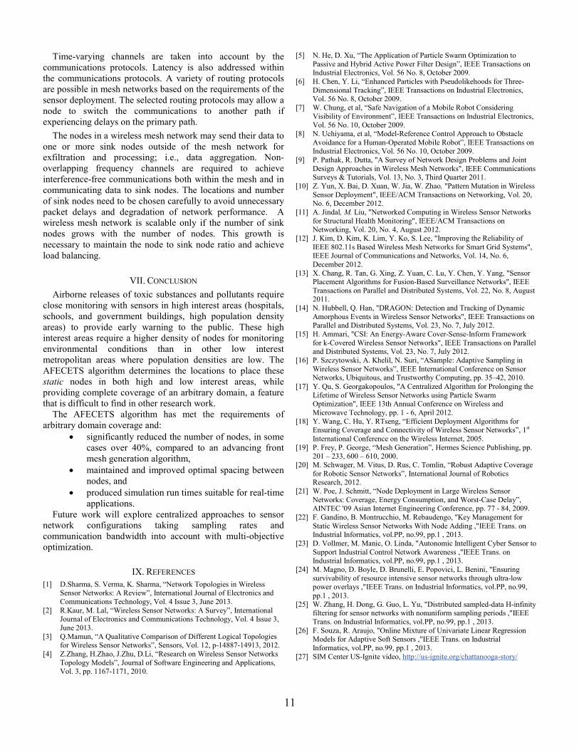
of the mesh network. Sensing range of the sensor affects the sensing coverage of the mesh network. Effective sensor deployment algorithms must consider both coverage and network connectivity. We use isotropic sensing and communications models, as well as a 2D equilateral triangular mesh deployment that provides maximum coverage with the smallest overlap and gap in coverage [23].
Each sensor in our mesh network has the same communications and sensing ranges. Two sensors, Si and Sj, are connected if cji RSS ≤ , where Rc is the communications
range of each sensor. The maximum coverage and no gap layout for nodes, as shown in Fig. 12, is when Sji RSS 3= ,
where Rs is the sensing range of each sensor. This is our optimal sensor layout resulting in full coverage with no sensing gaps in the sensor field and with minimal overlap in coverage. The area of coverage overlap between two sensors is the area of the intersection of two circles of radius RS.
Fig. 12. Optimal Sensor Layout with Sensor Spacing of SR3
A sensor spacing of Rs, or distance between sensors of CSji RRSS == also results in no gap coverage (see Fig. 13). A
sensor network deployment with these configuration parameters will require a larger number of sensors to cover the same area as in Fig. 12 because of greater coverage overlap and closer sensor spacing.
Fig. 13. Non-Optimal Sensor Layout with Sensor Spacing = RS
Therefore, two approaches for mitigating the problem of communications ranges affected by varying propagation conditions in the environment are: 1) utilize sensors that have a wireless communications range far greater than the distance to their neighboring sensors, and 2) increase the density of sensors in areas that experience high, or varying, signal degradation resulting in coverage overlap.
11
Time-varying channels are taken into account by the communications protocols. Latency is also addressed within the communications protocols. A variety of routing protocols are possible in mesh networks based on the requirements of the sensor deployment. The selected routing protocols may allow a node to switch the communications to another path if experiencing delays on the primary path.
The nodes in a wireless mesh network may send their data to one or more sink nodes outside of the mesh network for exfiltration and processing; i.e., data aggregation. Non-overlapping frequency channels are required to achieve interference-free communications both within the mesh and in communicating data to sink nodes. The locations and number of sink nodes need to be chosen carefully to avoid unnecessary packet delays and degradation of network performance. A wireless mesh network is scalable only if the number of sink nodes grows with the number of nodes. This growth is necessary to maintain the node to sink node ratio and achieve load balancing.
VII. CONCLUSION Airborne releases of toxic substances and pollutants require
close monitoring with sensors in high interest areas (hospitals, schools, and government buildings, high population density areas) to provide early warning to the public. These high interest areas require a higher density of nodes for monitoring environmental conditions than in other low interest metropolitan areas where population densities are low. The AFECETS algorithm determines the locations to place these static nodes in both high and low interest areas, while providing complete coverage of an arbitrary domain, a feature that is difficult to find in other research work.
The AFECETS algorithm has met the requirements of arbitrary domain coverage and:
• significantly reduced the number of nodes, in some cases over 40%, compared to an advancing front mesh generation algorithm,
• maintained and improved optimal spacing between nodes, and
• produced simulation run times suitable for real-time applications.
Future work will explore centralized approaches to sensor network configurations taking sampling rates and communication bandwidth into account with multi-objective optimization.
IX. REFERENCES
[1] D.Sharma, S. Verma, K. Sharma, “Network Topologies in Wireless Sensor Networks: A Review”, International Journal of Electronics and Communications Technology, Vol. 4 Issue 3, June 2013.
[2] R.Kaur, M. Lal, “Wireless Sensor Networks: A Survey”, International Journal of Electronics and Communications Technology, Vol. 4 Issue 3, June 2013.
[3] Q.Mamun, “A Qualitative Comparison of Different Logical Topologies for Wireless Sensor Networks”, Sensors, Vol. 12, p-14887-14913, 2012.
[4] Z.Zhang, H.Zhao, J.Zhu, D.Li, “Research on Wireless Sensor Networks Topology Models”, Journal of Software Engineering and Applications, Vol. 3, pp. 1167-1171, 2010.
[5] N. He, D. Xu, “The Application of Particle Swarm Optimization to Passive and Hybrid Active Power Filter Design”, IEEE Transactions on Industrial Electronics, Vol. 56 No. 8, October 2009.
[6] H. Chen, Y. Li, “Enhanced Particles with Pseudolikehoods for Three-Dimensional Tracking”, IEEE Transactions on Industrial Electronics, Vol. 56 No. 8, October 2009.
[7] W. Chung, et al, “Safe Navigation of a Mobile Robot Considering Visibility of Environment”, IEEE Transactions on Industrial Electronics, Vol. 56 No. 10, October 2009.
[8] N. Uchiyama, et al, “Model-Reference Control Approach to Obstacle Avoidance for a Human-Operated Mobile Robot”, IEEE Transactions on Industrial Electronics, Vol. 56 No. 10, October 2009.
[9] P. Pathak, R. Dutta, "A Survey of Network Design Problems and Joint Design Approaches in Wireless Mesh Networks", IEEE Communications Surveys & Tutorials, Vol. 13, No. 3, Third Quarter 2011.
[10] Z. Yun, X. Bai, D. Xuan, W. Jia, W. Zhao, "Pattern Mutation in Wireless Sensor Deployment", IEEE/ACM Transactions on Networking, Vol. 20, No. 6, December 2012.
[11] A. Jindal, M. Liu, "Networked Computing in Wireless Sensor Networks for Structural Health Monitoring", IEEE/ACM Transactions on Networking, Vol. 20, No. 4, August 2012.
[12] J. Kim, D. Kim, K. Lim, Y. Ko, S. Lee, "Improving the Reliability of IEEE 802.11s Based Wireless Mesh Networks for Smart Grid Systems", IEEE Journal of Communications and Networks, Vol. 14, No. 6, December 2012.
[13] X. Chang, R. Tan, G. Xing, Z. Yuan, C. Lu, Y. Chen, Y. Yang, "Sensor Placement Algorithms for Fusion-Based Surveillance Networks", IEEE Transactions on Parallel and Distributed Systems, Vol. 22, No. 8, August 2011.
[14] N. Hubbell, Q. Han, "DRAGON: Detection and Tracking of Dynamic Amorphous Events in Wireless Sensor Networks", IEEE Transactions on Parallel and Distributed Systems, Vol. 23, No. 7, July 2012.
[15] H. Ammari, "CSI: An Energy-Aware Cover-Sense-Inform Framework for k-Covered Wireless Sensor Networks", IEEE Transactions on Parallel and Distributed Systems, Vol. 23, No. 7, July 2012.
[16] P. Szczytowski, A. Khelil, N. Suri, “ASample: Adaptive Sampling in Wireless Sensor Networks”, IEEE International Conference on Sensor Networks, Ubiquitous, and Trustworthy Computing, pp. 35–42, 2010.
[17] Y. Qu, S. Georgakopoulos, "A Centralized Algorithm for Prolonging the Lifetime of Wireless Sensor Networks using Particle Swarm Optimization", IEEE 13th Annual Conference on Wireless and Microwave Technology, pp. 1 - 6, April 2012.
[18] Y. Wang, C. Hu, Y. RTseng, “Efficient Deployment Algorithms for Ensuring Coverage and Connectivity of Wireless Sensor Networks”, 1st International Conference on the Wireless Internet, 2005.
[19] P. Frey, P. George, “Mesh Generation”, Hermes Science Publishing, pp. 201 – 233, 600 – 610, 2000.
[20] M. Schwager, M. Vitus, D. Rus, C. Tomlin, “Robust Adaptive Coverage for Robotic Sensor Networks”, International Journal of Robotics Research, 2012.
[21] W. Poe, J. Schmitt, “Node Deployment in Large Wireless Sensor Networks: Coverage, Energy Consumption, and Worst-Case Delay”, AINTEC '09 Asian Internet Engineering Conference, pp. 77 - 84, 2009.
[22] F. Gandino, B. Montrucchio, M. Rebaudengo, "Key Management for Static Wireless Sensor Networks With Node Adding ,"IEEE Trans. on Industrial Informatics, vol.PP, no.99, pp.1 , 2013.
[23] D. Vollmer, M. Manic, O. Linda, "Autonomic Intelligent Cyber Sensor to Support Industrial Control Network Awareness ,"IEEE Trans. on Industrial Informatics, vol.PP, no.99, pp.1 , 2013.
[24] M. Magno, D. Boyle, D. Brunelli, E. Popovici, L. Benini, "Ensuring survivability of resource intensive sensor networks through ultra-low power overlays ,"IEEE Trans. on Industrial Informatics, vol.PP, no.99, pp.1 , 2013.
[25] W. Zhang, H. Dong, G. Guo, L. Yu, "Distributed sampled-data H-infinity filtering for sensor networks with nonuniform sampling periods ,"IEEE Trans. on Industrial Informatics, vol.PP, no.99, pp.1 , 2013.
[26] F. Souza, R. Araujo, "Online Mixture of Univariate Linear Regression Models for Adaptive Soft Sensors ,"IEEE Trans. on Industrial Informatics, vol.PP, no.99, pp.1 , 2013.
[27] SIM Center US-Ignite video, http://us-ignite.org/chattanooga-story/
12
[28] P. Lindstrom, “Model Simplification using Image and Geometry-Based Metrics”, PhD Dissertation, Georgia Institute of Technology, November 28, 2000.
[29] H. Mahboubi, K. Moezzi, A.G. Aghdam, K. Sayrafian-Pour, V. Marbukh, "Distributed Deployment Algorithms for Improved Coverage in a Network of Wireless Mobile Sensors ,"Industrial Informatics, IEEE Transactions on, vol. 10, no. 1, pp. 163-174 , Feb. 2014.
[30] Jianwei Niu, Long Cheng, Yu Gu, Lei Shu, S.K. Das, "R3E: Reliable Reactive Routing Enhancement for Wireless Sensor Networks ,"Industrial Informatics, IEEE Transactions on, vol. 10, no. 1, pp. 784-794 , Feb. 2014.
[31] Li Jia, R.J. Radke, "Using Time-of-Flight Measurements for Privacy-Preserving Tracking in a Smart Room ,"Industrial Informatics, IEEE Transactions on, vol. 10, no. 1, pp. 689-696 , Feb. 2014.
[32] M. Magno, D. Boyle, D. Brunelli, E. Popovici, L. Benini, "Ensuring Survivability of Resource-Intensive Sensor Networks Through Ultra-Low Power Overlays ,"Industrial Informatics, IEEE Transactions on, vol. 10, no. 2, pp. 946-956 , May 2014.
[33] K. Derr, M. Manic, “Wireless Sensor Network Configuration, Part I: Centralized Algorithms”, IEEE Transactions on Industrial Informatics, January 2013.
[34] S. Nawaz, S. Jha, “A Graph Drawing Approach to Sensor Network Localization”, IEEE International Conference on Mobile Adhoc and Sensor Systems, pp. 1 – 12, October 2007.
[35] K. Derr, M. Manic, “Adaptive Control Parameters for Dispersal of Multi-Agent Mobile Ad Hoc Network (MANET) Swarms”, IEEE Transactions on Industrial Informatics, October 2012.
[36] Plant Layout Plans, http://www.conceptdraw.com/solution-park/building-plant-layout-plans.
[37] Plant Engineering, http://www.juki.co.jp/industrial_e/customer_e/plant_e/.
Kurt Kurt Derr (M’04): Kurt Derr, IEEE Member, received the B.S. degree in electrical engineering from Florida Institute of Technology, M.S. degree in
computer science from the University of Idaho, and the Ph.D. degree in computer science from the University of Idaho (2013). Kurt is a Computer Scientist at the Idaho National Laboratory and has taught courses as Affiliate Faculty at the University of Idaho. He received an R&D 100 award in 2009 for RFinity, Mobile Open-Encryption Platform and has co-authored 7 patents. Kurt has also written a book, Applying OMT, on object-oriented technology. He has recent published papers at IEEE conferences and journals on swarm intelligence, wireless
communications, computational intelligence, and computational geometry in wireless networking environments. Milos Manic, PhD (S'95-M'05-SM'06): Milos Manic is a Professor with Computer Science Department and Director of Modern Heuristics Research
Group at Virginia Commonwealth University. He has over 20 years of academic and industrial experience. His previous positions include tenured positions with University of Idaho, University of Nis, Serbia, director of the Computer Science Program at Idaho Falls, and Fellow of the Brain Korea 21 Program, Seoul. As principal investigator he lead number of research grants with the National Science Foundation, Idaho EPSCoR, Dept. of Energy, Idaho National Laboratory, Dept. of Air Force, in the area of data mining and computational intelligence applications in process control, network
security and infrastructure protection. Dr. Manic is currently serving as IEEE Industrial Electronics Society (IES) Officer and is involved in various capacities in Technical Committees on Education, Industrial Informatics, Factory Automation, Smart Grids, Standards, and is a co-founder and chair of Technical Committee on Resilience and Security in Industry. Dr. Manic is an associate editor of the Trans. on Industrial Electronics, Trans. on Industrial Informatics, and Int. Journal of Engineering Education. He serves various IEEE conferences yearly in various capacities as a General Co-Chair,
Technical Program Chair, Track Chair, and Special Session Chair (ISRCS, IECON, ICELIE, HSI, INDIN, ICIEA, ISIE). Dr. Manic has published over 140 refereed articles in international journals, books, and conferences.