WIREI.ESS ENGINliER - americanradiohistory.comamericanradiohistory.com/Archive-Experimental Wireless/40s/Wireless... · WIREI.ESS ENGINliER ... to some fallacy in the treatment of

WIREI.ESS ENGINliER

Vol. XXV DECEMBER 1948 No. 303

Relatively -moving Charge and Coil

IN our September Editorial we considered some problems raised by Professor Cullwick and in this number we publish a letter in

which he discusses some of the points raised therein. He agrees that the e.m.f. induced in the coil should depend solely on the relative velocity of the coil and charge and not on which of the two one regards as moving and which at rest, and yet he finds difficulties - in applying classical theory to the case of the stationary charge and moving coil ; that is, as the phenomenon appears to an observer on the charge. In our opinion, his difficulties are largely due to a misconception of the nature of the electrostatic charges induced on the ring of wire as it approaches and recedes from the stationary charge.

His Fig. i is correct but his Fig. 2 is quite fallacious. He says that ` if the coil is a single loop of thin wire, negative charges will be induced on the outer surface in the neighbourhood of A, and positive charges on the inner surface.' This is quite wrong, as can be seen from our Fig. i in which a ring of wire is situated between two conducting surfâces, of which the upper is charged positively and the lower negatively. Lines of force will leave the upper conductor as shown and end on negative charges on the ring. These induced negative charges will be con- centrated towards the upper outside of the ring but will be distributed to some extent over the whole upper half of the ring as shown. The positive charges do not retreat to the inside of the ring but to the lower half. In Professor Cullwick's case the arrangement is not so symmetrical but the distribution is roughly the same ; that is a

negative charge on the surface of the ring in the neighbourhood of the stationary positive charge and a positive charge distributed over the more distant parts of the ring's surface, as we explained in the Editorial. The distribution is, of course, such that all parts of the ring are at the same potential. Consequently no line of electric force can go from one part of the ring to another part. We emphasise this because we suspect that Professor Cullwick pictured lines crossing the space inside the ring between his internal charges.

+ To an observer on the '(''(i'í'í 'ç"í'r'(YS' stationary charge these

\,.g.// / induced charges are moving with the ring

+ ® + and act as current ele - i +/ ,+ + \ / its \ ments, setting up a ,), ),l,), magnetic field. This

magnetic field will be a maximum through the ring at the moment of

nearest approach to the stationary charge. A moment ago there was no magnetic flux through the ring and a moment later the ring will have moved away from the stationary charge and the flux will again be zero. Would Maxwell have agreed that this magnetic flux could be smuggled somehow in and out of the ring without inducing an e.m.f. in it ? We disagree entirely with the statement that a logical application of Maxwell's equations seems to show that no e.m.f. is induced by the surface charges. In our opinion there is no inconsistency to be resolved by an application of Einstein's theory.

Professor Cullwick then propounds another

(a) (b) Fig. I

WIRELESS ENGINEER, DECEMBER i948 375

problem in which a charge is moving along the axis of a closed toroidal coil, but we must confess that we cannot follow his argument. With reference to his Fig. 4 he says, the induced current as it grows will induce an electric field along the axis of the toroid in the direction of motion of Q,' but the changing magnetic flux in the toroid not only induces an e.m.f. in the wire but also in the surrounding space, and it is difficult to see how the induced electric field along the axis can be in opposition to E as he infers. The electrostatic forces will certainly accelerate the moving element as it approaches and retard it as it recedes. If the resistance of the toroid is negligible no appreciable magnetic flux will be able to penetrate it, a negligibly small induced e.m.f. sufficing to produce the current necessary to maintain the resultant flux at zero.

Professor Cullwick also discusses the peculiar case in which the current in the toroid is maintained constant by some external source. In this case the magnetic flux due to the moving charge is simply superimposed upon that of the constant current, the induced e.m.f. being counterbalanced by variation of the externally applied voltage. This involves the supply or withdrawal of energy by the external source. Professor Cullwick states that as Q moves along the axis of the coil it experiences no magnetic or induced force whatever, whereas it exerts a magnetic force of repulsion on the toroid. He does not give his reasons for these conclusions, and one cannot help wondering if the apparent anomalies are due to some fallacy in the treatment of the problem.

It is an easy matter to overlook some little

ex - detail in such can lex problems. As an example we will take the

.-+M

case of the positive charge Q at rest and ® the toroid approaching it as shown in Fig. 2 (a). At the moment that the toroid passes the charge, as shown in Fig. 2 (b), there will

be an induced negative charge on the inner part and an induced positive charge on the outer part, and as these are moving to the left they will set up a magnetic field as shown, which reaches its maximum value at this moment. If the current is maintained constant by an external source of e.m.f. this magnetic field will grow as the toroid approaches and decrease as it recedes without experiencing any opposing m.m.f. As the toroid approaches, the growing magnetic flux will induce an e.m.f. in the direction shown

(a) Fig. 2

376

(b)

in any closed path linking the toroid. The externally adjusted voltage applied to the coil may prevent this induced e.m.f. affecting the current in the coil but it does not affect the induced e.m.f. in the surrounding space. The charge Q being at rest has only an electric field and this electric field will be distorted by the electric field induced by the changing flux. The direction of the induced field at Q is such as to repel it, but the induced electric field will also distort the electric field of Q in the neighbourhood of the toroid. The distorted electric field will exert a lateral pressure on the toroid tending to oppose its motion. In other words, the distortion of the electric field by the increasing magnetic flux produces a repellent force between the charge and the toroid. When the toroid has passed the charge the magnetic flux decreases, the induced e.m.f. is reversed and the force is still repellent ;

it thus always acts in opposition to the attractive electrostatic forces. To an observer on the coil the charge is moving and his description of the phenomena would be somewhat different, but any measurable quantity must surely be the same.

Fig. 3 may help to explain the nature of the force of repulsion between the charge and the toroid. This figure may represent two entirely different phenomena. It may represent the cross-section of a conductor carrying current towards the reader in a magnetic field, which is distorted as shown by the magnetic force due to the current. It may, however, represent an electric field in which the dots indicate a magnetic flux towards the reader. If this magnetic flux is decreasing it will induce an electric field left-handedly around it which will distort the original electric field as shown. Superimposed on this will be fields due to electric charges on conductors, but these present no difficulties. Just as the mechanical forces of repulsion in the magnetic case are transmitted to the body of the magnet and to the conductor, so in the electric case the force will be transmitted to the charge Q from which the electric field emanates and to the toroid which causes the distortion. The moral of all this is that, on dis- covering apparent anomalies in the application of classical theory to electromagnetic problems, one should not invoke Einstein or Ritz but examine very carefully one's fundamental con- cepts and their application.

We trust that these remarks will have thrown some light on what is undoubtedly a very in- triguing problem.

G.W. O. H.

WIRELESS ENGINEER, DECEMBER 1948

ANALYSIS OF BRIDGE -TYPE VALVE VOLTMETERS

By P. Popper, B.Sc., and G. White, B.Sc.

SIIMMARY.-An analysis is made of four arrangements of the bridge -type valve voltmeter, and a comparison is made from the point of view of sensitivity and h.t. stability. While in the case of a single -valve circuit, transference of the resistor from anode to cathode lead offers some advantages with respect to stability and linearity, this is not the case in the two -valve circuit. For the latter, a solution for non-linear operation is given.

1. Introduction WHEN a valve is used for the measurement

of direct voltages, it is desirable to balance out in some manner the steady

component of anode current since this allows the use of a more sensitive output meter, and also the whole of the scale becomes available for the indication of the input voltage. One method of achieving this is to make the valve and its associated resistors form two of the arms of a Wheatstone bridge. The other two arms are formed either by two resistors or by a similar valve and resistor. These two types of bridge amplifier can be further subdivided according as the valve resistor is placed in the anode or cathode circuit.

Various claims have appeared in recent literature regarding the advantages of placing the valve resistor in the cathode circuit, and of using two valves, but no comprehensive comparison of the four types of amplifier has yet been made.

Fig. 1. Single -valve circuit with anods resistor.

It is the purpose of this paper to compare the four types of amplifier from the point of view of sensitivity, stability, and linearity, and to find how the choice of the output meter affects the performance of these circuits.

MS accepted by the Editor, July 1947


2. Type I.-One Valve ; Anode Resistor Fig. i shows a single -valve bridge amplifier in

which the valve resistor is placed in the anode circuit, and the output meter is connected between anode and a tap on the potential divider R,R2.

V,

Fig. 2. Typical valve characteristic, linear over the

working range.

Now if the valve characteristics are assumed to be straight and parallel to each other over the working range, as shown in Fig. 2, the anode current is given by

I -Va+µV9-E0 (I) a ra where la, Va, ra, V9 and p, have the usual significance, and Eo is the intercept on the Va axis made by the tangent to the Vg = o curve.

Thus Va = raja + (Eo - F.Vs) .. .. (2)

This indicates that the valve can be replaced by an equivalent circuit consisting of a resistor ra in series with an e.m.f. given by Eo -µVg. Fig. 3, therefore, represents the equivalent circuit of the arrangement of Fig. i, provided the meter is omitted.

The open circuit voltage between A and B is given by

377

VBR1R+2 R2

1E0-µVg+ ra R+ya(VB--Eo-{- µVg)

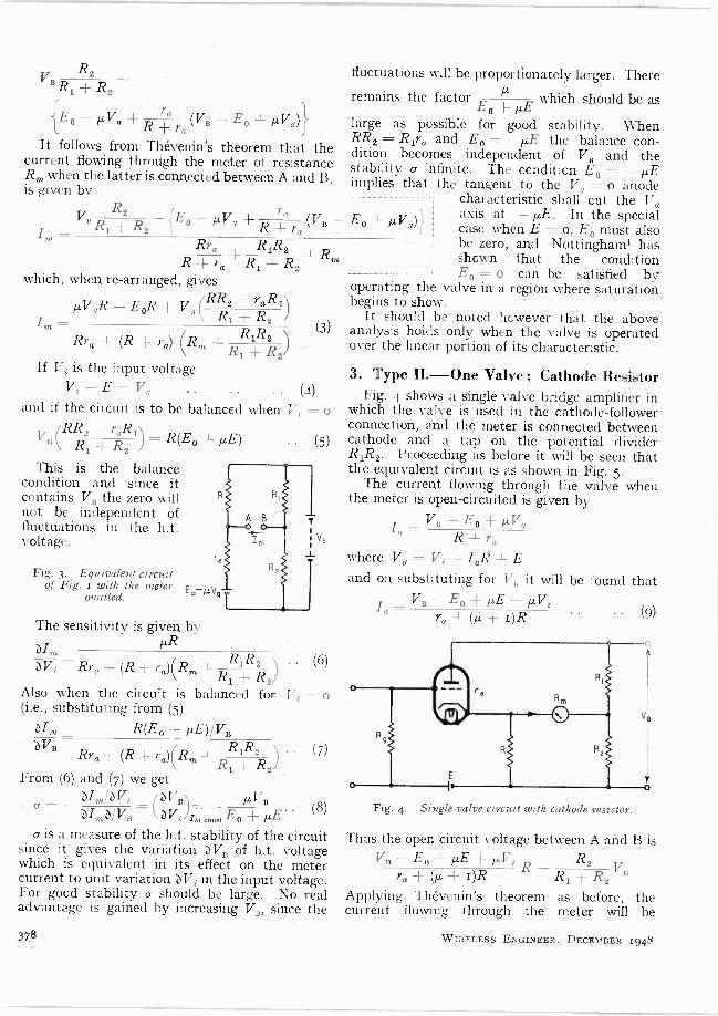
It follows from Thévenin's theorem that the current flowing through the meter of resistance Rm when the latter is connected between A and B, is given by

ra (VB V R2 B f Eo -µVg + R

I n - Rra RIRL

R+ ram RI+R2+Rm which, when re -arranged, gives

µVgR - EoR VB (RR2 - raR1)

l, Rra + (R + ra) (Rm - RIR2

\ R1 + R2/ If Vi is the input voltage

Vi -E=Vg (4)

(3)

and if the circuit is to be balanced when Vi = o

Ri - raRll

VB( R1+R2 J=R(Eo+µE) This is the balance

condition and since it contains VB the zero will not be independent of fluctuations in the h.t. voltage.

Fig. 3. Equivalent circuit of Fig. 1 with the meter Eo µV, omitted.

(5)

The sensitivity is given by

calm µR

W, Rra + (R + ra)(Rrn + RIR2 (6) R1+ R2) Also when the circuit is balanced for V; - o (i.e., substituting from (5)

Im R(Eo + µE)I VB WB

Rra + (R + ra)(Rm +\ . .

R1 R2/I

From (6) and (7) we get Z)Im/Z)Vi c)VB_ µ.VB

(V) I E Q=-

m conet 0+ µE

(7)

(8)

cr is a measure of the h.t. stability of the circuit since it gives the variation VB of h.t. voltage which is equivalent in its effect on the meter current to unit variation Z) V, in the input voltage. For good stability o should be large. No real advantage is gained by increasing VB, since the

37$

fluctuations will be proportionately larger. There

remains the factor µ which should be as Eo+µE large as possible for good stability. When RR2 = Rira and E _ -µE the balance condition becomes independent of VB and the stability cr infinite. The condition Eo = - µE implies that the tangent to the Vg = o anode

characteristic shall cut the Va axis at - µE. In the special case when E = o, Eo must also be zero, and Nottingham' has shown that the condition Eo = o can be satisfied by

operating the valve in a region where saturation begins to show.

It should be noted however that the above analysis holds only when the valve is operated over the linear portion of its characteristic.

E+µVg)}

3. Type ll.-One Valve ; Cathode Resistor Fig. 4 shows a single -valve bridge amplifier in

which the valve is used in the cathode -follower connection, and the meter is connected between cathode and a tap on the potential divider R,R2. Proceeding as before it will be seen that the equivalent circuit is as shown in Fig. 5.

The current flowing through the valve when the meter is open -circuited is given by

la=VB-EO+µVg R+ra where Vg = Vi - IaR + E and on substituting for Vg it will be found that

I -VB-E°+µE+µVi a ra+(µ+r)R .. (9)

Fig. 4. Single -valve circuit with cathode resistor.

Thus the open -circuit voltage between A and B is VB-E+µE+µVin R2

ra + (µ + r)R RI + R2 B

Applying Thévenin's theorem as before, the current flowing through the meter will be

WIRELESS ENGINEER. DECEMBER 1948

VB-E± !LE +µVi R2 ra+(µ+1)R R

RI-I-RZVB I- m RIR2 Ryal (µ + I) Ra,+ Ri + R2 + ral (µ + 1) + R

where R ral (µ + 1)

+ I) + R is the output impedance

ral(µ

of the cathode follower. On re -arrangement this gives

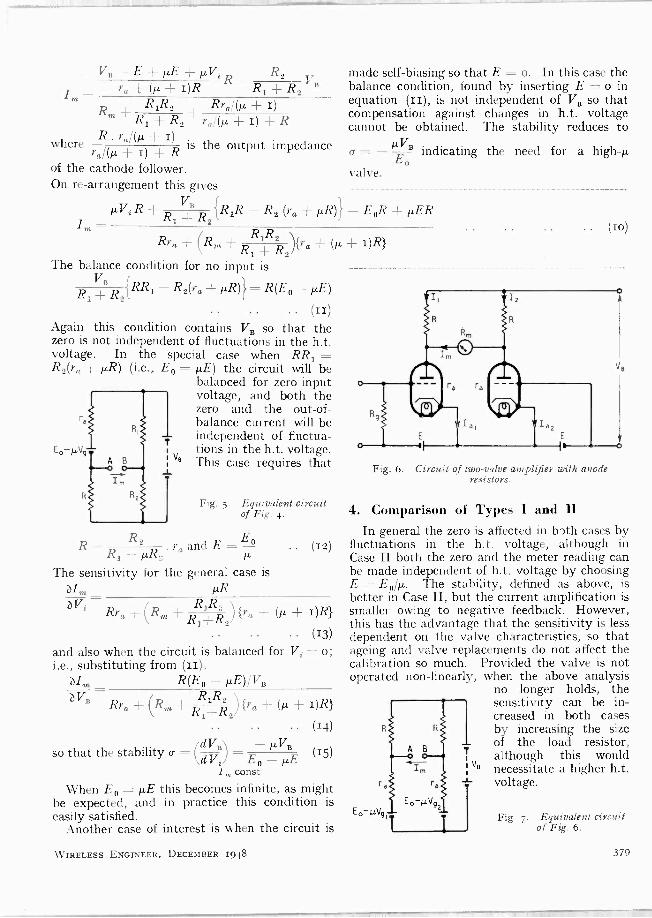
made self -biasing so that E = o. In this case the balance condition, found by inserting E = o in equation (ii), is not independent of VB so that compensation against changes in h.t. voltage cannot be obtained. The stability reduces to

a = -É B indicating the need for a high-µ 0

valve.

.. T7 D I Y B {Ri"? T)n n (

_. i R) l r n + r ri Im -

Rra + (Rm + RR+ R2){ra + (µ + The balance condition for no input is

+ R2{RRI - R2(ra + µR)} = R(E0 - µE)

Again this condition contains VB so that the zero is not independent of fluctuations in the h.t. voltage. In the special case when RRI = R2(ra + µR) (i.e., E0 = µE) the circuit will be

balanced for zero input voltage, and both the zero and the out -of - balance current will be independent of fluctua-

E0- µV9 tions in the h.t. voltage. This case requires that

Fig. 5. Equivalent circuit of Fig. 4.

R= R2 raandE=E0 RI -µR2'

The sensitivity for the general case is µR

Rra + (Rm + RR +R2)

{Ta - (µ + 1)R}

(13)

and also when the circuit is balanced for Vi = o; i.e., substituting from (ii).

Um R(E0 - µE)/VB 17,3

Rya H- (RT, 4 RIR2

) {ra + (µ + i)R} RI+R2 .. .. (14)

VB so that the stability v = (dV3) E0 µµE (15)

1 n const

When E0 = µE this becomes infinite, as might be expected, and in practice this condition is easily satisfied.

Another case of interest is when the circuit is

(iz)

WIRELESS ENGINEER, DECEMBER I948

I)R}

Fig. 6. Circuit of two -valve amplifier with anode resistors.

4. Comparison of Types I and 11

In general the zero is affected in hlth cases by fluctuations in the h.t. voltage, although in Case II both the zero and the meter reading can be made independent of h.t. voltage by choosing E = E0/µ. The stability, defined as above, is better in Case II, but the current amplification is smaller owing to negative feedback. However, this has the advantage that the sensitivity is less dependent on the valve characteristics, so that ageing and valve replacements do not affect the calibration so much. Provided the valve is not operated non -linearly, when the above analysis

no longer holds, the sensitivity can be increased in both cases by increasing the size of the load resistor,

7 although this would Ve necessitate a higher h.t.

ra y voltage.

Eo- µV91

A B

Im

E.-µV92

I


379

.i iu71tl ii il

5. Type III.-Two Valves; Anode Resistors Fig. 6 shows a double -valve bridge amplifier

in which two identical valves are used and the resistors are placed in the anode circuit. The equivalent circuit of this arrangement is shown in Fig. 7. The open circuit voltage between A and B is

(VB -Eo+µVg2)R+1,0

(VB -Eo+µ R Vgl) R R ra

µR =R+ra(Vg2-Vg1)

µVtiR R + ra

so that the current flowing through the meter is, by Thévenin's theorem, given by

R µVi

I - R+ra R

2Rra R

m +

-- ra

µRVi 2Rra + Rm (R + ra)

Since this equation does not contain VB the output current is independent of h.t. voltage.

Fig. 8. Two -valve circuit with cathode resistors.

Also In, = o when Vi = o so that under ideal conditions the circuit will be automatically balanced. The sensitivity is given by

r1l m µR Wi 2Rra + Rm(R + ra)

and the limit of J,/)Vi for Rm approaching zero is gm/2.

This shows that when Rm is small the most suitable type of valve for this arrangement is one of high slope. The stability cr for this circuit is infinite, since a.,/ Vi = o, indicating that fluctuations in the h.t. voltage produce only second -order variations in the output current.

(161

6. Type IV.-Two Valves; Cathode Resistors Fig. 8 shows a double -valve bridge amplifier

employing cathode resistors2 and two batteries E to bring the grids to a suitable operating point. The equivalent circuit is shown in Fig. 9. The current flowing through the left-hand valve with AB on open circuit is

IaI-VB-Eo+µV01 R + ra

where Val =Vi-Ia1R+E which gives

IaI-VB-Eo+µE+µVi ra + (µ +i) R

Similarly Ia2 - VB - Eo + µE ra + (µ ± I)R

Hence the open -circuit voltage between A and B is

µRVÈ V"B ra+ (IL +1)E

Applying Thévenin's theorem, the output current µR Vi

ra 1)R Im

YAP' + 1) + R

µRVi or /,, = 2Rra + Rm {ra + (µ + I)R} ( 18)

Again this equation does not contain VB, so that the output current is independent of h.t. voltage. Also, as before the circuit is automatically balanced when Vi = o.

The sensitivity t)I m µR

Rm 2Rral (f.c + I)

(17)

2Rra + Rm {ra + (µ + I)R} ' ' (19)

and the limit of liImdV, for Rm approaching zero is gm/2 as before.

Equation (is) can be very easily derived if the circuit is replaced by an equivalent constant - current generator gm Vi working into the circuit of Fig. Io.

As can be seen, the current flowing through the branch Rm when Rm = o is given by gmVi/2, and in this case there is no stabilizing action due to negative


feedback. On the other hand with Rm large and ra/R small cIo/Vj- I/Rm showing all the advantages of full negative feedback.

Eo-µV

380 WIRELESS ENGINEER, DECEMBER 1948

7. Comparison of Types III and IV

In both cases fluctuations in h.t. voltage produce second -order effects only. Also from the¡formulae (i6) and (ig), it can be seen that theisensitivity is greater with Type III than with Type IV. As with Types I and II, the sensitivity can be increased by increasing the size of the load resistors, and the h.t. voltage, provided the valves are not operated non -linearly, when the analysis is not valid. When the meter resistance is small the sensitivity in both cases tends to gm/2, showing the need for a high -slope valve.

9mVi

Fig. io Circuit equivalent to Fig. 8 when fed by a constant -current generator.

8. Non-linear Operation When the valves are operated non -linearly the

response is more easily determined by graphical than analytical methods. The procedure in Cases I and II will be described briefly, but the more important Cases III and IV will be dealt with fully. Case I

The response of this circuit can readily be determined by plotting on the characteristics of the valve the load line corresponding to the effective anode resistor, which is

R(RRR,I+R2R2

m + )

R Rm RIR2 RI+R2

The change in the voltage produced across the effective anode resistor by a given input voltage can then be read from the characteristics, and the output current determined by dividing this

voltage by Rm + R1 + R2

Case II. The response in this case can be determined in

the normal way as for cathode followers. The dynamic characteristic for a resistor

R{Rm + R1R2/(RI + R2)} R + Rm + RIR2/(RI + R2)

is first plotted, and since this effective resistor is in the cathode circuit, the voltage produced across it by various input voltages can be found by plotting on the dynamic characteristic the

load lines corresponding to the input voltages. The output current is then given by the voltage produced across the effective cathode resistor

divided by Rm -f- RR +R2.

The effective

cathode resistor has a linearizing effect on the response in this type as with the normal cathode follower.

Case III. When this circuit is operated non -linearly the

response curve is best determined by assuming various values for the current flowing through the second valve, which operates up and down the anode characteristic corresponding to the steady biasing voltage on its grid. The anode voltage Va2 on this valve can be determined from this characteristic when Ia2 is known. The voltage drop VB2 across the second anode resistor, the current I2 flowing through it, the meter current Im, the anode voltage Vai on valve (i), the voltage drop VRi across the first anode resistor, the current Ii flowing through it, and the anode current Iai flowing in valve (i) can then all be calculated from the following equations :

VR2 = VB - Va2 .. (21) T

12 = Y R2/R2 (22)

Im =I2-Ia2 (23)

Lai = Va2 -Rm'm (24) VRi = VB - Vai (25)

II = V.1/Ri (26)

Iai =lm+Ii (27)

4

3

E

E

z

CASE IY (HIGHER WORKING POINT)

4,5"" 2 3

Vi (VOLTS)

Fig. i i. Experimental and calculated amplifier characteristics.

O EXPERIMENTAL POINTS CASE TQ

II 11

and thus since Iai, Vai are known, read from the valve characteristics be calculated from

V.=VBi+E

4

11

Vg, can be and Vs can

(28)

WIRELESS ENGINEER, DECEMBER 1948 381

Hence by choosing certain values for Ide, a series of values for Im and V1, can be obtained.

Practical Example. Table I shows the results obtained using the

above method for an ECC32 valve. The h.t.

I=I2-Ia2 IIR, = I,R2 + I mRms

Ial=II+Im Val=VB-RI, ..

and since Val, Ial are known,

TABLE I

(3r) (32) (33) (34)

Vg1 can be read

Ia2 (mA)

Vag (volts)

VR2 (volts)

I2 (mA)

Im (mA)

Val (volts)

VR1 (volts)

I1 (mA)

4, (mA)

Vol -

(volts) V1

(volts)

3.45 218.0 69.o 3.45 0 218.0 69.o 3.45 3.45 - 4.85 0 3.25 214.0 73.0 3.65 0.40 214.0 73.0 3.65 4.05 - 4.42 0.43 3.00 210.0 77.0 3.85 0.85 210.0 77.0 3.85 4.70 - 3.98 0.87 2.75 205.0 82.o 4.10 1.35 205.0 82.0 4.10 5.45 - 3.50 1.35 2.5o 200.0 87.0 4.35 1.85 200.0 87.0 4.35 6.20 - 3.00 1.85 2.25 196.0 91.0 4.55 2.30 196.0 91.0 4.55 6.85 - 2.6o 2.25 2.00 190.0 97.0 4.85 2.85 190.0 97.0 4.85 7.7o - 2.05 2.8o 1.75 184.0 103.0 5.15 3.40 184.0 103.0 5.15 8.55 - 1.47 3.38 1.50 178.o 109.0 5.45 3.95 178.0 109.0 5.45 9.4o - 1.00 3.85 1.25 172.0 115.0 5.75 4.50 172.0 115.0 5.75 10.25 - 0.40 4.45

TABLE II

12 (mA)

Vg2 (volts)

Vae (volts)

422Im (mA) (mA)

Ii (mA)

Iai (mA)

Vai (volts)

Val (volts)

Vi (volts)

3.45 - 4.85 218.0 3.45 0 3.45 3.45 218.o - 4.85 0 3.47 - 5.25 217.6 2.74 0.73 3.47 4.20 217.6 - 4.44 0.81 3.49 - 5.65 217.2 2.11 1.38 3.49 4.87 217.2 - 4.13 1.52 3.51 - 6.05 216.8 1.58 1.93 3.51 5.44 216.8 3.84 2.21 3.53 - 6.45 216.4 1.05 2.48 3.53 6.o1 216.4 - 3.6o 2.85 3.55 - 6.85 216.0 0.65 2.90 3.55 6.45 216.o - 3.40 3.45 3.57 - 7.25 225.6 0.35 3.22 3.57 6.79 215.6 - 3.24 4.01 3.59 - 7.65 215.2 0.05 3.54 3.59 7.13 215.2 - 3.08 4.57

voltage was assumed to be 287 volts and the anode resistors 20,000 ohms. The grids were assumed to be biased to - 4.85 V, a suitable operating voltage, and the output meter was taken as o-5 mA meter with a resistance of 5 ohms.

The graph of Fig. ri shows the output current Im plotted against Vi as calculated by this method together with experimental points. As can b e seen the response is practically linear over the range considered, and the experimental points lie very close to the calculated curve.

Case IV. The response in this case is best determined by

assuming various values for the current I2 flowing in the second cathode resistor. Using the nota- tion of Fig. 8, Vat, V,,, can now be calculated from the equations

Vat = VB - RI2 .. (29) Vg2=E-RI, .. .. (3o)

Now since Vat and V92 are known Ia2 can be read off from the valve characteristics. Im, Il, Ial, and Val can then be calculated from the following equations

382

from the valve characteristics. V1 can then be determined from

Vi V +RI, -E.. (35) Thus by choosing certain values for 42, a

series of values for Im and V2 can be obtained.

Practical Example. Table II shows the results obtained using the

above method for an ECC32 valve. The same working point, load resistors and output meter have been assumed as before.

The lower graph in Fig. ri shows the calculated output current Im plotted against V1, together with experimental points, and as can be seen the response is far from linear. This is because the second valve is driven nearly into cut-off, while the first valve is driven towards V9, = o by an amount which is roughly half the input voltage. Thus compared with the previous case, the working range for linear response is reduced, and a better working point would be in the region of - 2.50 V. An experimental sensitivity curve which was obtained using the latter working point is also shown by the upper graph in Fig. xi. The departure from linearity is approximately


the same as in Case III which is never greater than 1% of full-scale deflection up to inputs of 3 volts, while within the range 3-4 volts Case III is slightly more linear.

Thus the arrangement employing anode resistors is equivalent, as far as linearity is. concerned, to that employing cathode resistors with due consideration to the optimum working point.

9. Choice of Output Meter So far, the expression lI,m/ZVi has been taken

as the criterion of sensitivity, but this is not necessarily the only one. Since the final indication is an angular deflection, perhaps a better criterion would be the Deflection Sensitivity defined by

Deflection sensitivity -Angular deflection

Or Input voltage

S = Im/Vi .. .. (36) where 4, = meter sensitivity in degrees deflection per µA. Approximately

= kVRra so that

S = k1/R . I/Vi (38)

(37)

Differentiation of this expression with respect to Rm shows that S is a maximum when

2R NIm o m' N?,{N.91. Vi ci Vi (39)

Applying this equation to all four cases it is easy to find the optimum meter resistance R°m. It will be found that in

Case I Rya RIR2

R° R+ra+RI+R2 (40)

Case II 12º,= Ryal(µ '+ 1) + RIR2

(41) R + ra RI + R2

Case III. i

Case III 2Rra R+ra

Case IV 2Rral (µ + 1)

R° (43)

te` R+yl(F+1) .

Thus in all four cases, optimum performancefis obtained when the meter resistance is equal to the output impedance of the circuit ; i.e., when maximum power is delivered. In actual practice this condition is only easy to satisfy in Case IV where the optimum value R°m is comparatively low.

0'7 :

N> A A

0'6

0

0

0

09

CASE

e1111111111

u . ..111 .a

511 CASE u AFTEN AGING)

51,',1` II,'', CAS .A\\,.

C \\_ ... 1413.1133.......,\.SE AFTE ..

.5 ...U.....'\_R AGING S 1,000

R,,, (n) Fig. 12. Effect of meter resistance on sensitivity.

To find how exactly the choice of Rm affects the sensitivity N-,,pVi and the deflection sensitivity S in Cases III and IV; a calculation was made for the ECC32, assuming that

µ = 32

gm = 2.3 mA/V.

ra = 14,000 Sì.

It was also assumed that R = ra in both cases. The results are tabulated below.

(42)

0.20 500 1.500 2,000

R,,, 20 5° 100 200 500 1000 2000

Um/c V, S/k

I.14 1.14 1.13 1.13

5.1 8.1 11.3

1.10 15,9 24.6

0.07 1.00

33.7 44.8

Case IV.

R, 20 50 100 200 500 824 1000 2000

ÚI,,dVi .. I.I2 5.0

I.o8 1.02 7.6

0.92 10.2 13.0

_ 0.71 05.9

0.58 16.45

0.52 0.33 16.4 14.9


The graph of Fig. 12 shows the sensitivity Im/Z2Vi plotted against Rm for the two cases.

In each case bI,m/AVi - g,,,/2 as Rm->o. The graph illustrates well the superiority of Type III where sensitivity is concerned.

Fig. 13 shows the deflection sensitivity plotted against Rm for Cases III and IV, and Case IV shows very well that there is an optimum value for the meter resistance. The optimum value for Case III is 14,000 ohms, clearly not a practical value.

The calculations just given were repeated for R = 2ra and R = 3ra, and in both cases it was found that the alterations in the response curves were negligible over the range of Rm considered. The effect of aging of the valves was also investigated by assuming a drop in the mutual conductance from 2.3o to 1.15 mA/V together with a corresponding increase in the anode characteristic resistance from 14,000 to 28,000 S2.

Tne sensitivity v . R,,, curves were recalculated for Cases III and IV and these are plotted in Fig. 12. As can be seen the calibration in Case IV approaches its original value as the value of R0 is increased to a much greater extent than in Case III. This is due to the fact that in Case IV, as R,a is increased the negative feedback increases tending to make the calibration less dependent on the characteristics of the valves.

10. Current Measurement All the circuits previously described may be

used for the measurement of current. The current is passed through the grid resistor of the input valve and a voltage is produced which gives a deflection as before. The current amplification obtainable can be derived in each case by multiplying the sensitivity by the value R9 of the grid resistor ;

cilm Im i.e., R9

(Vi Thus the larger the grid resistor, the larger the

current amplification. There are, however, limitations to the size of the grid resistor due to the flow of grid current.'

11. Conclusions The analysis shows that with the single -valve

type of voltmeter independence of h.t. voltage variations cannot be obtained, except when the load resistor is placed in the cathode circuit of the valve together with a positive biasing battery of value E =µE6. In the case of the two valve type of voltmeter independence of h.t. voltage

(44)

variation is obtained only if the two valves are identical.

The statement' that the linearity of the double - valve circuit is increased by the use of cathode resistors in place of anode resistors is shown to be at variance with our findings.

Thus while it appears that in the single -valve circuit the placing of R in the cathode lead has some advantage, this does not appear to be the case in the two -valve circuit.

s k

50

40

30

20

CASE IY

5 0 1,000

R,, (n)

Fig. 13. Effect of meter resistance on deflection sensitivity.

1,500 2.000

If the deflection sensitivity is taken as the criterion of performance then optimum results are obtained when the meter resistance is equal to the output resistance of the circuit used. This condition cannot be realized in practice in the double -valve circuit with anode resistors.

Finally if a o-ioo µA meter is used with an ECC32 valve in the recommended arrangement an input voltage of approximately 4 mV will produce an output current of 5µA.

12. Acknowledgment The authors wish to thank J. A. M. van Moll

and the Directors of Philips Electrical Ltd., for permission to publish this work.

REFERENCES Nottingham, J. Franklin Inst., 1930, Vol. 209, p. 287.

s Chapman, Phys. Rev., 1/15 Sept. 1944, Vol. 66, No. 5/6. Simmons, U.S. Patent 2,360.523. Nielsen, Rev. Sci. Inst., 1947, Vol. 18, p. 18.

384 WIRELESS ENGINEER, DECEMBER i948

MUTUAL IMPEDANCE OF TWO CENTRE -DRIVEN PARALLEL AERIALS

By B. Starnecki and E. Fitch (Signals Research and Development Establishment, Ministry of Supply)

SIIMMARY.-A formula and'curves are given for the mutual impedance between two symmetrically -placed parallel aerials assuming a sinusoidal distribution of aerial current. The values are shown to be in fair agreement with measurements.

1. Introduction T is known that a system of two aerials may

be represented by the equivalent network shown in Fig. i. In this figure Z11 and Z22

are the self -impedances of the two aerials, measured at the terminals ; Z12 is the mutual impedance between them ; generators with e.m.f.s E9 and E1 with internal impedances Z9 and Z1 are applied at the terminals of the respective aerials. If the loop -currents (the currents at the terminals) are II and I2, the network equations are :

Z11II+Z1212=E9-Z9I1 Z121I+Z2212=E1 -Z1I2

The currents at the aerial terminals may be evaluated from these equations provided that all the impedances are known.

Z11 Z12 Z22 -Z12

Fig. I. Equivalent circuit of two aerials.

It is important to note that Z11 and Z22 are the self -impedances of the aerials which differ, in general, from the ' intrinsic ' impedances. The intrinsic impedance is the input impedance of a single aerial in free space ; its value for symmetrically driven aerials may be calculated from existing formulaeL 2, 3 The self -impedance is the input impedance of the aerial in the presence of the other aerial with open -circuited terminals ;

this has not yet been evaluated, but for practical use the difference between the intrinsic and self -impedance can usually be neglected provided that the spacing of the aerials is not too small*.

Values of the mutual impedance Z12 of two

WIRELESS ENGINEER, DECEMBER I948

parallel aerials of equal length have been calculated (Ref. i, page 372).

A general formula for two infinitely thin aerials has been derived by J. Aharoni at S.R.D.E., and a description of his method can be found in his book4. From this theory, assuming that the distribution of aerial current is sinusoidal, J. H. Tait at S.R.D.E. has derived practical formulaet for two symmetrically -driven parallel aerials, not necessarily of equal length, with terminals lying on a line perpendicular to the aerials ; this paper records the results obtained.

2. Computation of Mutual Impedance The formulae obtained by Tait are

sin kl1 sin k12 R12 30

cos k (1, + 12)[2 Ci p - Ci s - Ci t + Ci u -Ciq+Ciy - Cie]

+ sin k(11+12)[-Sis+Sit+Siu-Siq - Si y + Si r] + cos k (1, - 12)[2 Ci p - Ci s -Cit+Cix - Ci r + Ci w - Ci q] + sin k(11-12)[Sis-Sit-Six+Sir

+ Si w - Si q]

sin klt sin kl2

X12 30 cos k (1, + 12)[- 2Si p + Si s + Si t - Si u

+ Siq-Siy+Sir] + sin k (1, + 12)[- Ci s + Ci t + Ci u - Ci q - Ci y + Ci r] + cos k(1,-12)[-2Siß+Sis+Sit-Six

+ Si r - Si w + Si q]

+ sin k (l1 - 12)[Cis - Cit- Cix+Cir + Ciw - Ciq]

* It should be noted that sometimes the effect of the other aerial cannot be neglected. For example, suppose that the first aerial is a half -wavelength dipole and the second a full -wavelength dipole. Then when the latter is open -circuited the influence of the half -wavelength wires on the first aerial maybe great.

tTwo papers have recently appeared giving the same formula as that quoted here, namely, C. Russel Cox, " Mutual Impedance between Vertical Antennas of Unequal Heights ", Proc. Inst. Radio Engrs, November 1947, Vol. 35, No, Is, p. 1367, and Giorgio Barzilai, Mutual Impedance of Parallel Aerials ", Wireless Engineer, November 1948, Vol. 25. No. 302, P. 343.

385

where kd k[1/1,2 + d2 + l,] k[V1,2 + d2 - l,] k[s/122 + d2 + 12]

k[s/122 + d2 - 12]

k[1/(11 + 12)2 + d2 + (1, + 12)] k[s/(11 + 12)2 + d2 -

(11 + 12)]

k[1/(11 - 12)2 + d2 + (11 - 12)]

k[1/(11 - 12)2 + d2 - (11 - 12)] and

=p =q = r = s

= =n =v = w

=x

Z12 = R12 + 9X,2 k = 27r/A

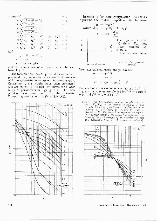
A = wavelength and the significance of l,, l2 and d can be seen from Fig. 2.

The formulae are too complicated for immediate practical use, especially since small differences of large quantities may appear in computation. Consequently the results have been computed and are shown in the form of curves for a wide range of parameters in Figs. 3 to 7. The computation was done partly by the Scientific Computing Service and partly at S.R.D.E.

1.000

100

s

N

O

386

\\ Fig 3(a)

OL

0.101

1

\

` \ .,

2.8

2-4

zo

1.6

14

I.2

1.0

\ 0.8 \

0.6

04

IELD OF \ \ ELEMENTARY

\. 0.1

10

0-2

In order to facilitate interpolation, the curves represent the mutual impedance in the form

Z12 - I,Z/121 e2°

1z121 = V 81.22 + X,22.

O = tan -1 X12

I

1,

where

R,2 The figures lettered (a) show IZ12I and i those lettered (b)

__j show O.

The curves have

Fig. 2. Two parallel d -1 aerials.

been normalized, using the parameters = 27x1,/.1

= 27rd/A ß

(b° = 9o° -30o- - B°

Each set of curves is for one value of 11/12 (= I, 1.5, 2, 3, 4). Curves are plotted for 1,/A = 0.016 to 0.45 and d/.l = 0.032 to 1.6

Fig. 3. (a) The modulus and (b) the phase Bl2 = tan -1X12/R12 of the mutual impedance of two parallel dipoles of equal length 1 as a function of the spacing d. a = 27x1/À, ß = 27rd/.1, 56° = 9o° - 36o d/A - 0°. The dotted lines represent an asymptotic approximation ; the chain line represents the phase of the field strength of an elementary dipole at a distance d from it. (The scale is arbitrary).

'0-8

\`

3(

Fig.3(b)

,.0

Iz

\ \\ IC

\Y`\\\ I4

I6

228 24

'

`\\ I , . \.. \ I\

I\,

a 28

2.4 ID

\ rX I 6 PHASE OF \\I4 I2

I.0

ELDIPÓLÉRY

. 0I 10

ß

o

0

oo


100

10

N

0.1

(3

0 1

11111 eke,

lelesS11111 LitiellhäLthilit,

2 0

08

II

10

Fig.4 (a)

2.7

2.4

2.1

1.8

1.5

I.2

0.9

0.75

0.6

0.45

0.3

0.1

1.2

1.5

1.8

2.1 2.4 2.7

0. a 0.15 0.45 0.6 0.75

I

i

.ß

10 300

Fig.4 (b)

0

2.4 2.I

I8 I.5

.1.2 0.9

100

10

3

Fig. 4. (a) The modulus and (b) the phase 012 = tan -1X,2/R12 of the mutual impedance of two parallel dipoles of lengths ll and l2 = 4/I.5 as a function of the spacing d. a = zlrll/A ; ß = 27rd/A ; rk° = 90° - 360 d/A - 0°. The dotted lines repre-

sent an asymptotic approximation. Fig. 5. (a) The modulus and (b) the phase 012 = tan 1 X12/R12 of the mutual impedance of two

parallel dipoles of lengths la and l2 = 11/2 as a function of the spacing d. a = 2al,/À ; ß = 2.rrd/A ; 4)° = 9o° - 36o diA - 0°. The dotted lines

represent an asymptotic approximation.

0.1

CC =1.0 1.2 1.4

1.6

2.0

2.4 2.8

0.1

0.2 0.4 0.6 0.8

Fig. 5(b)

a `2.8

2.4

1 2.0

1.

I46 \1.2 I0

10

300

03

10

3

95°

o°


521

100

10 30

10

N

Fig. 6 (a)

10

0.1

500

gill 111111 4

11111 h

1113131121111511,

yee:111; ai

15

a 27

2.4

21

1.8

1.5

1.2

09

075

0.6

0.45

0.3

100

0.101

388

10

0'I

1.2

o

1.5

1.8

2'1

2.4

2.7

9

-

a 0 15 0-45 06 0'75

10

Fig. (b)

30300

a - . 2.7 2.4 \ 2.1 1.8 1.5 12 0'9

100

10

3

Fig. 6., (a) The modulus and (b) the phase 012 = tan' X12/R12 of the mutual impedance of two parallel dipoles of lengths ll and la = ll/3 as a function of the spacing d. a = 21T11/Á ; ß = 222d/À ; t° = 90° - 36o d/A - B°. The dotted lines represent

an asymptotic approximation. Fig. 7. (a) The modulus and (b) the phase 012 =

tan -1 X 12/R12 of the mutual impedance of two parallel dipoles of lengths ll and 12 = ll/4 as a function of the spacing d. a = 22211/A ; ß = 21rd/A ; #° = 90° - 36o d/A - 0°. The dotted lines

represent an asymptotic approximation. 300

100

10

3

95°


The broken lines show the asymptotic value of IZ121 for wide spacing d,

r2O hit tan Z12I = kd tan

2 tan

2 0° = 90° - 36o d/A

A feature of the curves is the rapid increase in mutual impedance for small separations and short aerials. This may be ascribed to the increasing influence of the induction field. For purposes of comparison the ,field in the plane of symmetry of an elementary dipole has been plotted in Fig. 3 (chain line) with arbitrary scale. It may be seen that . the behaviour of the field strength of such a dipole is quite similar to that of the mutual impedance.

3. Comparison with Experiment The values obtained from the curves given

above have been checked experimentally. An extensive series of measurements has been made by N. P. Quinlivan at S.R.D.E. using vertical aerials mounted above a horizontal

y

6

4

2

C

o

0 + ° e

e

0

o

O

e

- e

o o e°

o

°

e e

0 a8°

e ° ° eo

o

0 0

8eeo - .. ®er

60 gr 20 40 60

EXPERIMENTAL

BO 100

scatter, especially for high values of impedance, the general trend seems satisfactory. (The product -moment correlation coefficient calculated for the points was found to be 0.94.). It should be noted that the experimental results were obtained for aerials which were, of course, not infinitely thin.

The method of measurement was as follows :- (a) The second aerial was removed and the

input impedance Z11 of the first aerial measured. (b) The first aerial was removed and the input

impedance Z22 of the second aerial measured. (c) The input impedance Zi of the first aerial

was measured with both aerials in position and the second aerial short-circuited.

(d) Assuming that the impedances measured in (a) and (b) are self -impedances (whereas they are in fact intrinsic impedances) the mutual impedance was calculated from

Z12 = [Z22 (Z11 - Zi) The assumption in (d) may have introduced

loo

ICJ, - 00 °

° 0 0

o

oA

°

8e

w-

o

0

EXPERIMENTAL

100

Fig. 8. Comparison between theoretical and experimental results ; (a) mutual resistance ; (b) mutual reactance.

earth mat (` G.L. mat ') of 4O0 -ft average dia- meter. The frequency range was 3 to 20 Mc/s. The accuracy of the measuring equipment was estimated to be of the order of io per cent.

The number of experimental points was usually insufficient to plot complete curves corresponding to the theoretical curves given in Figs. 3 to 7, but an overall comparison between the theoretical and experimental values of resistance and reactance is given in Fig. 8. The theoretical value is plotted against each experimental value obtained. It can be seen that though there is a considerable

some errors ; unfortunately, it was not possible to measure the self -impedances of the aerials owing to the practical difficulty of open -circuiting the aerials completely.

4. Acknowledgment The authors wish to thank the Chief Scientist,

Ministry of Supply for permission to publish. REFERENCES

° Schelkunoff, S. A. " Electromagnetic Waves," Van Nostrand, 1943. ° King, R. and Middleton D. Quarterly ofApplied Mathematics, January

1945. Vol. 1. ' Middleton, D. and King, R. J. Appl. Phys. April 1946. Vol. 17. ° Aharoni, J. " Antennae," Oxford, 1946:

WIRELESS ENGINEER, DECEMBER 1948 c 389

DIVERSITY RECEPTION IN U.S.W.

RADIO LINKS By Giorgio Barzilai, M.Sc. and Gaetano Latmiral

SUMMARY.-Some of the principal troubles, due to multipath transmission in ultra -short-wave radio links, are briefly reviewed, and it is shown how they can be avoided or reduced, when receiving at points of reinforcement.

Because the spatial distribution of interference maxima and minima is not stable, due to variation of the refractive index of the atmosphere, the use of several receiving aerials, suitably displaced, is considered. Criteria for the disposition of the receiving aerials, and for their connection to the receiver, are deduced. Finally these considerations are applied to a practical case.

1. Introduction IN ultra -short-wave radio links, the signals

reaching the receiving aerial usually arrive by two or more paths. If the ground between

and around the receiving and transmitting points is flat, and the receiving point is above the line of sight of the transmitter, the propagation will take place along two paths. In such a case a ' direct -ray ' and a ` ground -reflected ray ' are present. If, on the contrary, the ground between and around the receiving and transmitting points is rough, with hills, towers, buildings and other reradiating or reflecting obstacles, many ` rays '

will reach the receiving aerial along paths of different lengths. It may even happen that, because of intervening obstacles, only the direct ray can reach the receiver.

Also the tropospheric reflections, due to the sudden variations of the dielectric constant of the atmosphere with increase in height, contribute to the increase in the number of the received rays. These phenomena usually cause serious fading and distortion.

By using directional transmitting and receiving aerials the number of the received rays can be reduced, but it is not generally possible to eliminate totally the parasitic rays, leaving for example only the direct ray, as the resulting directivities would be so sharp as to make the radio link unstable, principally because of the variation of the atmospheric refractive index.

The simplest way of overcoming or reducing these difficulties, is to use a system of several suitably spaced receiving aerials. Such a system is effective with any type of modulation.

If directional aerials are used, and the propagation takes place over relatively flat ground, the direct ray and the ground -reflected ray are very strong, compared with the parasitic rays arising from tropospheric, or other reflections.

MS accepted by the Editor, July 1947

390

When a simple carrier, or a carrier modulated within a narrow frequency band is transmitted, interference occurs between the direct ray and the ground -reflected ray, so that in moving vertically, regions of reinforcement (field a maximum) and of cancellation (field a minimum) are encountered in turn. The minima are zeros, and the maxima regions of field strength double that of the direct wave, only when reflection occurs without change of amplitude. This is usually assumed to be the case in elementary treatments, both for horizontal and vertical polarization. The spatial distribution of maxima and minima is, however, not stable because of the variation of the atmospheric refractive index. This variation causes the equivalent radius of the earth to vary between 8,000 and rr,000 km. The dielectric constant of the atmosphere decreases with the height, the variation de/dh being usually of the order of i part in io,000 per kilometre. Assuming a certain variation of this gradient with time the rate of change of the spatial distribution of the maxima and minima depends on the ratio of the difference between the reflected and the direct path lengths to the wavelength. This is usually the origin of atmospheric fading. This fading generally has a long period, from several minutes to a few hours, because the variation of the average gradient de/dh is very slow.

Fading similar to the atmospheric fading, but due to tropospheric reflections, is particularly great when the receiving point is below the line of sight of the transmitter. The magnitude of this fading may reach 4odb, and its frequency several cycles per second.'

If instead of a single frequency, or a very narrow band of frequencies, a wide frequency band is transmitted, as in the case of television, it is possible to have the phenomenon of frequency distortion, simultaneously with and independently of the fading effect.


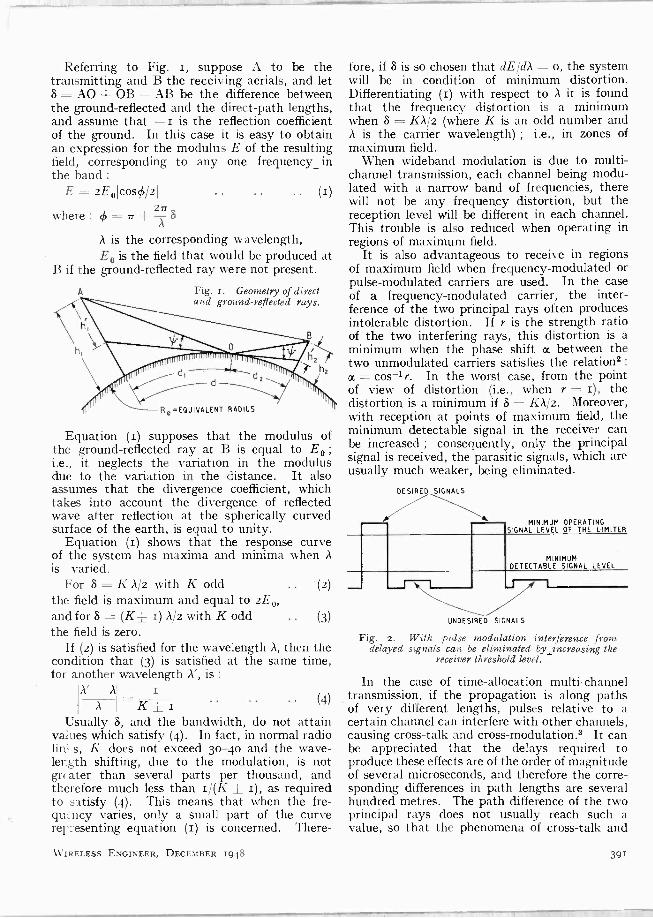
Referring to Fig. i, suppose A to be the transmitting and B the receiving aerials, and let 8 = AO + OB - AB be the difference between the ground -reflected and the direct -path lengths, and assume that -i is the reflection coefficient of the ground. In this case it is easy to obtain an expression for the modulus E of the resulting field, corresponding to any one frequency_ in the band :

E = 2EDIcos¢/2I

=Tr+ 8

A is the corresponding wavelength, E0 is the field that would be produced at

B if the ground -reflected ray were not present.

where :

A

.. (i)

Fig. 1. Geometry of direct and ground -reflected rays.

ReEQUIVALENT RADIUS

Equation (I) supposes that the modulus of the ground -reflected ray at B is equal to E0 ;

i.e., it neglects the variation in the modulus due to the variation in the distance. It also assumes that the divergence coefficient, which takes into account the divergence of reflected wave after reflection at the spherically curved surface of the earth, is equal to unity.

Equation (i) shows that the response curve of the system has maxima and minima when A

is varied. For 8 = K A/2 with K odd .. (2)

the field is maximum and equal to 2E0, and for 8 = (K± i) A/2 with K odd the field is zero.

If (2) is satisfied for the wavelength A, then the condition that (3) is satisfied at the same time, for another wavelength A', is :

A' -A i

A K±i Usually 8, and the bandwidth, do not attain

values which satisfy (4). In fact, in normal radio linl s, K does not exceed 30-4o and the wavelength shifting, due to the modulation, is not gr( ater than several parts per thousand, and therefore much less than i/(K ± i), as required to satisfy (4). This means that when the fre- quLncy varies, only a small part of the curve representing equation (r) is concerned. There -


(3)

.. (4)

fore, if 8 is so chosen that dE/dA = o, the system will be in condition of minimum distortion. Differentiating (i) with respect to A it is found that the frequency distortion is a minimum when 8 = KA/2 (where K is an odd number and A is the carrier wavelength) ; i.e., in zones of maximum field.

When wideband modulation is due to multichannel transmission, each channel being modulated with a narrow band of frequencies, there will not be any frequency distortion, but the reception level will be different in each channel. This trouble is also reduced when operating in regions of maximum field.

It is also advantageous to receive in regions of maximum field when frequency -modulated or pulse -modulated carriers are used. In the case of a frequency -modulated carrier, the interference of the two principal rays often produces intolerable distortion. If r is the strength ratio of the two interfering rays, this distortion is a minimum when the phase shift or. between the two unmodulated carriers satisfies the relation2 :

a = cos-lr. In the worst case, from the point of view of distortion (i.e., when r = I), the distortion is a minimum if 8 = KA/2. Moreover, with reception at points of maximum field, the minimum detectable signal in the receiver can be increased ; consequently, only the principal signal is received, the parasitic signals, which are usually much weaker, being eliminated.

DESIRED SIGNALS

nrninun vrcnMImu SIGNAL LEVEL 0F THE LIMITER

MINIMUM DETECTABLE SIGNAL LEVEL

2 I

UNDESIRED SIGNALS

Fig. 2. With pulse modulation interference from delayed signals can be eliminated by ..increasing the

receiver threshold level.

In the case of time -allocation multi -channel transmission, if the propagation is along paths of very different lengths, pulses relative to a certain channel can interfere with other channels, causing cross -talk and cross-modulation.3 It can be appreciated that the delays required to produce these effects are of the order of magnitude of several microseconds, and therefore the corresponding differences in path lengths are several hundred metres. The path difference of the two principal rays does not usually reach such a value, so that the phenomena of cross -talk and

391

I i u17IfIYI11II i 10 11 I Illít :i

cross -modulation will always be due to the parasitic signals mentioned above. By working at points of maximum field, it is possible, in this case also, to eliminate the undesired signals, by increasing the minimum detectable signal of the receiver as shown in Fig. 2.

simultaneously. In this way, by suitably proportioning the a.g.c. voltages, and by using special devices when receivers with limiters are employed,5 it can be ensured that only the systems corresponding to a field above a certain level are utilized.

S2

S

4

} Se

SI

(b)

S4

Se

Fig. 3. Methods of connecting three aerials (a) and four (b) to a receiver through relays.

2. Diversity Reception From the considerations given in the preceding

paragraph it is evidently of advantage to receive in those regions of space in which the interference of the two principal rays produces the maximum field. These regions, however, are moving, due to the variation of the atmospheric refractive index. As it does not seem to be practicable to ' chase ' these maxima, by moving the receiving parabolic mirrors, or horns, the most convenient solution is to use several suitably displaced receiving aerials and to arrange some electrical device to switch on the particular aerial situated in the maximum field.

This is substantially the same principle as that employed in ionospheric diversity reception, except that in this case the receiving systems are distributed in a horizontal plane, while in the atmospheric diversity reception they would be essentially distributed in the vertical direction.4 In practice, it suffices to distribute the aerials vertically, either by using suitable towers or by taking advantage of the natural slope of the ground. On occasion it is convenient, in order to avoid fading due to lateral reflections, to displace them laterally, rather than to place them in the same vertical line.

The various aerials could each be connected to a receiver, and the output of each receiver used to generate a negative a.g.c. voltage. This voltage must be proportional to the maximum input, and must be applied to all receivers

392

RECEIVER

This method is not always convenient, however, because in the case of multichannel transmission it is necessary to detect and combine each channel separately, and this causes serious complications in the terminal or repeater equipment. In addition, the simultaneous working of two or more receiving systems may increase the distortion, since, as already explained, the weaker signals are usually the more distorted.

It is more convenient, therefore, to use mechanical or electronic relays capable of switching on the system situated in the maximum field.5 These relays could be driven by auxiliary receivers designed to receive the complex wave, and they must be regulated in such a way that they only operate for a reasonable difference between the signals, in order to avoid instability.

In Fig. 3 (a) and (b) are sketched two possible ways of connecting the relays when three or four aerials are used. In (a), S1, S2, S3 represent three differential relays. Relay SI will switch into position I or 2 according to whether the signal received by the aerial AI is greater or less than the signal received by the aerial A2. Relay S2 will switch into position I or 3 according to whether the signal received by AI is greater or less than the signal received by A3. And similarly for relay S3. From the diagram it can be seen that only the aerial receiving the strongest signal will be connected to the receiver. The diagram of Fig. 3 (b) is similar except that it refers to four aerials, and consequently needs two


1'91 II 1,11111' 11141Ml

more relays. The case of two aerials is obvious. In order to establish the proper positions of the

receiving aerials, consider a radio link in which the receiving aerial is above the line of sight of the transmitter, take into account only the two principal rays, and refer to Fig. i.

When the atmospheric refractive index varies, the equivalent earth's radius varies according to the relation :

R8 r + (de/dh)R9Iz R° where R° is the earth's geometrical radius = 6370 km, and de/dh usually varies6 from - 0.63 x io -4 to - 1.36 x io -e. Consequently the projections h1' and h21, above the plane tangential to the surface of the earth at the reflection point, change and accordingly vary the path difference 8 and the field at B. Using well-known methods'' 8 it is possible to calculate 8 in terms of the increment dh2 of the height h2 of the receiving point, for each equivalent radius of the earth. Then curves of the field at B, for each equivalent radius, may be plotted against the increment dh2. It will thus be easy to determine the number of the aerials and their vertical displacement, in order to ensure that the field, at one of them at least, will never drop below a fixed fraction of the maximum field 2E0.

In the above, the divergence coefficient and the reflection coefficient of the ground were assumed to be equal to i and -i respectively. The moduli of these coefficients, however, are always less than unity, and the actual conditions are more favourable than those considered, for the oscilla- tions of the resulting field are smaller than those given by equation (r).

These considerations may now be applied to a practical case. Suppose that it is

Fig. 4. Curves relating El2E0 to dh'1 and dh'1 for 4h'2 and 4h'1 constant respectively.

E

2Eo

10

0"5

radio link is particularly interesting for Italian communications as it is one possible way of connecting Sardinia with the mainland. It . is not possible to use a direct link, because the receiving points would be below the line of the sight of the transmitters.

Referring to Fig. r, and increasing the height of the transmitting and receiving points by io m, in order to take into account the necessary installations, we have :

h1=1o2gm; h2=645m; d=gikm. To calculate h1', h2 and 8 the following approxi-

mate relations'', satisfactory in most practical cases, are used :

h'1 = h1 - d12/2R, .. (5) h'2 = h2 - d22/2R, .. .. (6)

h',/d, = his/d2 = tan 0 .. (7) 8 = 2h'1 h'2/d .. .. (8)

Using (5), (6), (7), and taking into account the fact that d = d1 + d2, it is easy to find, by trial and error, the values of h'1 and h'2, and then by (8) to calculate 8.

The results of this calculation are :

h'1=843m; h'2=562m; 8=10.4m; for R8 = 8,000 km.

d-91km ',f \_,.\, -4-

ao

¢ Q o 10

OR Ohi IN METRES

required to design an ultra -short-wave radio link between Monte Capanne (1019 m.a.s.l.)* in the isle of Elba, and Monte Argentario (635 m.a.s.l.). In this case the propagation takes place entirely above the sea, and therefore it is justifiable to take only the two principal rays into account when calculating the field at the receiver. This

m.a.s.l. = metres above sea level


128 13 .5

21:11

202

30

h'1=892m; h'2=586m; 8=II.5m; for Re = 11,000 km.

As can be seen, 8 varies by about 1.I m when the atmospheric refractive index changes from its maximum to its minimum value. Now if it is proposed to adopt a wavelength = 0.5 m, it follows that during the total variation of the atmospheric refractive index there will be two

393

cycles of fading. Obviously this happens either if the transmitting point is A and the receiving B, or if the receiving point is A and the transmitting B.

EMIN=2E°COs 45°=I 41E0

(a)

that 91, increases by d¢ = 180° from one to the other (i.e., dh'2 = 13.15 m) gives a condition such that the field on at least one aerial will not fall below 2E, cos 45° = 1.41E0.

A1

tos so°

EM,N=2E°cos so°=i 73E.

(b)

En -2E000S 22°30'..1e5E0

(c)

Fig. 5. Vector diagrams showing the composition of minimum signals for (a) two, (b) three, and (c) four aerials.

To establish the number of receiving aerials and their vertical displacement, suppose A is the transmitting, and B the receiving point. Increase h2 to h2 dh2 and find out, for a fixed value of Re, and using (5), (6), (7), (8) and (1), the value of the relative field E/2Eo. It is easy to verify, however, that as the increments h2 in the present case are very small in comparison with h2, the reflection point does not change appreciably when h2 increases by Ah 2. It is therefore possible to calculate 8 as if the propagation took place over a plane earth, between points situated at heights h'1 and h'2. In the present case the approximation introduces negligible errors, simplifies the calculation, and allows us to assume S to be proportional to Ah' 2. As only variations of S are concerned, and because of the proportionality, the curves of E/2Eo against dh'2 can be plotted starting from any arbitrary point on the vertical of the receiving point.

Suppose that dh'2 is measured from a point where E is a maximum. The patterns of the relative field E/2Eo are plotted in Fig. 4 against dh'2 for values of 8,000 km and ii,000 km for Re ; h'1 is taken as constant. For these values of Re, E varies from its maximum to its minimum value when dh'2 is 13.5 m and 12.8 m respectively. Taking the average of these values, it may be concluded that for a vertical displacement of 13.15 m the angle 4. of equation (1) increases by 180°. As the field is proportional to cos (A/2,

spacing the aerials by such a vertical distance

394

Inspection of Fig. 5 (a) makes this clearer. The two vectors OA, and OA, are supposed to rotate, maintaining their relative position, with the angle #/2 of equation (1). Therefore in this case they will rotate 360° more when the atmospheric refractive index changes from its maximum to its minimum value (A increases by 720°). The relative angle between OA, and 0A2 is equal to the increment 4¢/2 by which ¢/2 increases when moving from one aerial to the other. In this case, the increment is 90°. The projections of 0A1 and OA, on the horizontal axis are, therefore, proportional to E/2Eo relative to the two aerials. It is easy to see that the two vectors are drawn in the position corresponding to the minimum field. On both aerials the field is equal to 1.41E0.

The spacing of three aerials by such a vertical distance that 4. increases by AO = 120° from one to the next (i.e., dh'2 = 8.7 m), means that the field, on at least one of them, will not decrease below 2E, cos 30° = 1.73E0. Fig. 5 (b) relates to this case, and its interpretation is analogous to that of Fig. 5 (a).

Using four aerials with vertical separations such that (A increases by d¢. = 90° from one to the next (i.e., dh'2 = 6.6 m) the field, on at least one of them, will not decrease below 2E0 cos 22° Jo' = 1.85E, [Fig. 5 (c)]. Obviously, the nearer the value of the minimum tolerable field is to 2Eo, the greater is the number of aerials required, and the larger the total vertical distance


1. Introduction THE output of noise, either of impulse or

thermal type, from a linear amplifier is theoretically deducible from the overall

frequency characteristic (amplitude and phase) of the amplifier, without knowing the circuits or characteristics of each stage separately. This follows from the fact that the noise input may be written down in the form of a frequency spectrum, which is then operated upon by the amplifier overall characteristic to give the output noise spectrum.

MS accepted by the Editor, August 1947.


occupied. In the three cases examined, the total vertical distances occupied are about : 13.15 m, 17.4 m and 19.8 m respectively.

If B is the transmitting point, by a calculation similar to the preceding one, it will be found that for R.= 8,000 km, E changes from its maximum to its minimum value for a vertical increment

= 20.2 m, while for Re = il,000 km the increment Ah',- 19.4 m (Fig 4, curves h'2 = constant.) Therefore assuming, as before, a value corresponding to the average of the values relative to maximum and minimum equivalent radii, it can be concluded that the angle 9S in equation (1) increases by 18oß for a vertical increment of about 19.8 m. The three increments dh',, corresponding to the three dispositions considered above are : dh', = 19.8 m, dh', = 13.2 m and Ah', = 9.9 m respectively ; the three corresponding vertical distances occupied by the aerials are about 19.8 m, 26.4 m and 29.7 m.

3. Conclusion From these considerations it can be concluded

that the use of diversity reception in ultra - short -wave radio links has many notable advantages.

Atmospheric fading due to multipath transmission is completely avoided.9

Frequency distortion, when wideband modulated carriers are employed, is also reduced to a minimum.

Distortion, cross -talk and cross -modulation, that occur when frequency- or pulse -modulated carriers are used, due to the parasitic signals of

considerably less strength than the principal signal, are also eliminated, or reduced, by using a suitable a.g.c. system.

In the case of radio links between very high points the use of the diversity receiving system is thought to be essential in order to obtain stable radio links. This system is particularly convenient when the direct ray is of about the same strength as the indirect one ; this obviously occurs when the intervening country is flat ground or water'°,11

REFERENCES 1 C. R. Englund, A. B. Crawford and W. W. Mumford, " Ultra Short -

Wave Propagation," Bell Syst. tech. J., October 1938, p. 489.

' S. T. Meyers, " Nonlinearity in F.M. Radio Systems due to Multipath Propagation," Proc. Inst. Radio Enges, May 1948, p. 256.

' F. F. Roberts and J. C. Simmonds, " Multichannel Communication Systems," Wireless Enge, November 1945, p. 538.

' G. Latmiral and G. Barzilai, Italian Patent, Application Date 18th July 1946, Reg. 14, No. 228-Dispositivi per Ridurre le Evanescente e le

Distorsioni nei Collegamenti con Onde Cortissime tra Punti Elevati sul Suolo. ' British Patent No. 577,247-Improvements in Diversity Reception of Frequency -Modulated Signals.

' A. Bottini, " Ricerche sulla Constante Dielettrica della Bassa Atmos- fera," Boll tech. I.M.S.T., Gennaio-Febbraio 1943, p. 35.

° L. Sacco, " Note sui Ponti Radio (Simmetrici e Dissimetrici)," Ricerca Scientifica, Luglio-Novembre 1946.

' F. E. Terman, " Radio Engineers' Handbook," McGraw Hill Book Co.,

1943, p. 685. E. Labia, " Microwave Relay Radio Systems," Elect. Commun.,

June 1947, p. 131. 1° G. G. Gerlach, " A Microwave Communication System," R.C.A.

Review, December 1946, Vol. VII, No. 4, p. 576. 11 G. H. Huber, " Space Diversity Reception at Super High Frequencies"

Bell Lab. Rec., September 1947, Vol. XXV, No. 9, p. 337.

THERMAL NOISE OUTPUT IN

A.M. RECEIVERS Effect of Wide Pre -Detector Bandwidth

By M. V. Callendar, M.A.

On this basis, it is sometimes assumed that the overall characteristic of a complete radio receiver (as determined, for instance, by using a signal generator with variable frequency modulation) is sufficient to define the noise output. It might, for instance, be assumed that a change in i.f. bandwidth of a receiver from 20 kc/s to 200 kc/s would not alter the effective sensitivity (as determined by signal/noise ratio) provided there was no change in the audio acceptance band (say 5 kc/s).

It is, indeed, reasonable to imagine that, provided the signal carrier is much greater than the noise at the input to the detector, the various

395

I 11111 2) d i

components of the pre -detector noise spectrum may be regarded as sidebands giving beats with the carrier. But when the signal is smaller than the noise at the detector input, we shall be hearing ,the beats between the various noise components rather than betwecn them and the carrier. Under these conditions we might expect that an increase in pre -detector bandwidth would increase output noise even when the pre -detector bandwidth is much wider than the a.f. bandwidth. However, the problem is evidently not of a type readily soluble by simple or ' commonsense ' methods.

Thanks to the recent mathematical (mainly statistical) work of R. E. Burgess and others on the action of a rectifier on thermal noise, we are now in a position to obtain a reasonably complete answer to the problem so far as thermal noise in an a.m. receiver is concerned.

We cannot deal here with the allied problems of variation of noise with bandwidth in other cases-such as thermal noise in f.m., vision or pulse receivers, or impulse noise in any receiver, in the presence of signals. Though these problems have been attacked by numerous writers, there does not seem at the moment to be a sufficient mathematical basis available for a complete or exact solution of most of them. 2. Theory 2.I Circuit

A complete a.m. receiver may be represented as in Fig. I.

E, is r.m.s. signal at the rectifier. Fractional modulation is m.

E, is r.m.s. noise volts per unit of frequency at the rectifier, and is assumed uniform over the band B1.

En= E,/B1 is the total r.m.s. noise in the band B1, as measured at the rectifier.

A is the r.f. plus i.f. amplifier gain and is assumed to be uniform over the pass band of width B1 c/s and zero outside it. Thus, the signal at the aerial terminal is E,IA and the noise in the band B1 is E/A when referred to the aerial terminal.

V', and V' are r.m.s. noise and signal output from the rectifier, which is assumed to pass frequencies up to B1 without loss, but to remove the radio and/or intermediate frequencies.

V, and V are r.m.s. noise and signal output from the receiver, after passing through an a.f. filter and/or amplifier which is assumed to have unity gain up to a frequency B2, and zero gain beyond this. The filter may be considered to include the frequency characteristics of the post -rectifier filters, the a.f. amplifier and the loudspeaker. The gain in the a.f. amplifier will not, of course, affect the signal/noise ratio for a given frequency characteristic. Assuming only that B,> 2/32, any change in B1 will not affect the output noise pulse length, and V may reliably be taken as a measure of the audible loudness of the noise.

396

It is required to find V, and V for any given values of E,, E0, B1 and. B2. In particular, it is required to find whether V, and V are at all dependent upon the pre -detector bandwidth B1 in cases where B1>2B2.

A A

R F. AND I.F. AMPLIFIER

Es. En

DETECTOR

v5. A.F FILTER

AND AMPLIFIER

Vs V

BANDWIDTH B, ACCEPTANCE BAND B,

Fig. I. General form of an a.m. receiver.

2.2 Basis of Formula R. E. Burgess gives formulae for noise and

signal output from rectifiers in Radio Research Board Papers Nos. 93 and III. The formulae given below for V' and for V', and V, have been derived directly from those of Burgess by inserting the appropriate symbols for signal and noise inputs to the detector. The formulae for V are obtained from V' as follows :-

(i) For E,<0.25E approx. the output power spectrum is given by (i - f/B1)

2 J B(I

-f/BI)f whence V;` 2 = rs

Jo(r-f/BI)f 2B2\

I B2\ B 2B (ii) For Es>2E approx. the spectrum is

uniform up to 2-

1 and zero beyond this.

Thus V742 = 2B2, v,2 BI

assuming only that B2< B1 2

(iii) For intermediate values of ES/E, the spectrum is intermediate in form and not simply describable.

2.3 Linear Detector The internal impedance is assumed negligible.

(a) Signal< Noise (error < I db for E,< 0.25E) V'2=0.43 EóBI V2 = 0.43 Eó B2(2 - B2/BI) V,2 = V',2 = m2E,2 E82/EÓ Bi

(b) Signal i Noise (error<i db for Es> 2E) V'2 = E02B1 Vn2 = 2E02B2 V,2 = V',2 = m2Es2

(c) Signal and Noise of Same Order No exact formula available.


2.4 Square -Law Detector D.C. characteristic is V = aE2

(a) Signal <Noise (error < i db for E3 < 0.25En) V'n2 = 4a2E02BI2 Vn2 = 4a2E04B2(B1 - o.5B2) Vs2 = V'82= 8a2m2B 84

(b) Signal > Noise (error < r db for E,> 2En) V',.2 = 8a2E02E,2B1 Vn2 = 16a2Eo2E,2B2 Vs2 = V',2= 8a2m2Es4

(c) Signal and Noise of Same Order (general formula)

V',,2 = 4a2(2E82 + E02BI) Vn2 = 4a2(2E,2 + E02B1)E02B2(2 - B2/KB1) V,2 = V',2= 8a2m2B,4

Here K varies from i for En > E, to co for E,> En.

2.5 Signal/Noise Ratios Deriving now the output signal/noise ratio, we

have :- (a) Signal <Noise (E,<o.25En)

For Square -Law Rectifier V, mE,2 ./ r

Vn E02 B2(B1-o.5B2)

For Linear Rectifier V,

is as for square law n

except for a slight difference in the constant (+ 7%).

Signal> Noise(E,>2En) For either type of Rectifier

V, mE, mEsB1 0 V 2B2 En N 2B2

(b)

(c)

Vn E Signal and Noise of Same Order For Square -law Rectifier

V, mE, r Vn E0ß/2B2 VI .+ Eo2B1/2E,2

with a small correction (<r db) when 2B2 approaches B1;

For Linear Rectifier no exact formulæ are available, but results are probably very similar.

2.6 Signal/Noise ratio v. Bandwidth From the formulæ we may summarize the way

in which the signal/noise ratio varies with B1 as follows (we assume only that B1>2B2) :-

(a) When the signal is materially greater than the noise at the rectifier input, the signal/


noise ratio is always unaffected by the pre - detector bandwidth B1.

(b) When the signal is much smaller than the noise at the rectifier, the signal/noise voltage ratio is proportional to

I/V(Bl - o.5B2). In the case of the square -law detector, this variation in signal/noise ratio is due to the fact that the noise output volts increases as VB1 - o.5B2; with a linear detector, on the other hand, the noise output is unaffected by B1, but the signal modulation is suppressed to a degree dependent upon En and hence upon B1.

(c) As the bandwidth B1 is increased, starting from B1 = 2B2, the signal/noise ratio for a given signal will not start to fall until the noise (Eoi,/B1) voltage at the detector rises to half the signal voltage at that point.

(d) Since Vg

= 1.4m / B1 when En 0.5E,, V NNNB2' we see that a reduction of B1 will not improve signal/noise ratio except on signals so weak that the noise output exceeds that given by VB2/2B1 x r00% modulation of the signal. The improvement will not be really noticeable in practice unless the noise is' some io db above this level.

2.7 Graphical Presentation of Results Figs. 2 and 3 exhibit the relations in graphical

form. They should be used in conjunction with the following notes :-

(i) Noise output for values of B2 other than io4 may be obtained by multiplying noise figures obtained from the graphs . by I0-2 -/B2. The form of the curves is unaltered.

(ii) The graphs, with the above extension, hold for any values of B1 and B2, provided that B1>2B2 (apart from the small error not exceeding r db which occurs when E,>E, and B1 approaches 2B2).

(iii) Though B1 does not appear explicitly in Fig. 3, it must be borne in mind that En is proportional to ß/B1.

(iv) The rectifier in Fig. 3 is assumed linear when E, or En exceeds I.o volt, and square law, with a = 0.9, when E, and E2 are both below 0.2 volt. These figures are typical for diode detectors.

(v) The curved portions of the graphs representing values of input between 0.2 and

397

rQmurruw

z.0 volt, and values of E/E3 between 0.25 and 2.0, must be regarded as approximate only. Little purpose would, in any case, be served by attempting a high accuracy here, since practical detectors will deviate appreciably from the ideal types, especially near the transition region between parabolic and linear rectification.

ll oo E l

CC

>q> ` 10

Ñ

of this paper ; the threshold signal at the aerial terminal is approximately equal to the noise (in the band B1) referred to the same point.

It is worth noting that the signal/noise ratio of signals below the threshold could be improved by adding a synthetic carrier at the receiver, though its synchronization might be difficult.

3. Practical Conclusions As a practical case, we may first take

a typical t.r.f. television sound receiver, with relatively high fidelity a.f. amplifier and loudspeaker reproducing up to ro kc/s. If the r.f. bandwidth is i Mc/s for -6 db, a reducticn in bandwidth will only improve signal/noise ratio in the case of transmissions where the r.m.s. noise output exceeds that from about 7% modu-

Es -225Ói:::::::::ií:::.:iii:i 3".9.;!:".."'"12::::::M/4 MIA ..... Eoliii:8111.1111uIMIPT.d IMMINI111uZIOTAIZIM111n M.uulNBIB.:iä/M111111111r 1.11 RIBMO111111111.22:IIIÍIMM111 1-11111 1.1.1E11EIIIIII1111111.11111I1./_Mi ÍI IMR111M

INE11111II =28103 o==_:::::.::::

.::::: ::::: ::.......... 11111 . 1111 ...u. ....u. 11.0.11IMBIM.r11rrOR.11M..... EffiSi11111111111111C:IIIII 1111111111IIIII11111II lSi111111111111111' 111ffl11111li"!11111""I111111

ffl::::::1M::c::I=::::II=13=::2::I _ o ou o n u _ o o . u m IMMI111111311111111111MMII11111MM11111 IIIIII111111IIIIII111111

EEII1111111111IEE1111111E111111t111111E111111E111111 11111111MIIIIIIIIMt111111IIMt111111

002 01 10 10

PRE-DETECTOR BANDWIDTH B (Mcls)

2.8. Effect of Pre -detector Bandwidth If we; consider instead the change of out-

put signal/noise ratio with signal level E,: the formula show that, for normal signal levels, such that E8>2E,,, the signal/noise ratio varies as i/E3, but when ES falls below o.25E the signal/noise ratio varies as r/Es2. Thus there exists a threshold value of signal level below which the output signal/noise ratio deteriorates rapidly. This threshold is analagous to the better known threshold levels found in analyses of frequency - modulated or pulse -modulated signals : in all cases the threshold occurs when the signal amplitude is of the same order as the noise at the detector, but the phenomenon is more noticeable in practice with f.m. and p.m. receivers owing to the ' capture effect ' exerted by the noise once the signal is below threshold, and to the wider bandwidth usually employed there.

We also see that, whereas the signal/noise ratio for normal signal levels is controlled by the post - detector bandwidth B2, this threshold level is controlled by the pre -detector bandwidth BI and is unaffected by B2. It is the ratio BI/B2 that determines whether the threshold occurs at a level where the signal/noise ratio would otherwise be acceptable, or whether the threshold signal would be too poor for intelligible reception.

The actual signal field level for threshold depends, of course, upon factors outside the scope

398

loo

IO

Fig. 2 (left). Variation of noise1'ignal ratio with pre -detector bandwidth. For an a.f. bandwidth (B2) of Io kc/s, at various values

of signal carrier.

Fig. 3 (below). Variation of noise and signal with signal input to the rectifier. For an a. f. bandwidth (B2) of so ke/s, with various values of noise input (F2.---- E0y'B,) to the rectifier.

.:::::ffl.:::::::.:: -NOISE imm.11111 Mor...

IIMM.nEuIIIIIM y L1111 igi ---SIGNAL r..rllOr. , r111 IMIZ311111fflMIIIIIII JZIIIII IIIIII

I.0!>EI11III. Ena V'I -'r 17Si i11111 .. . .....C'.'.s: ::::I ....J'.[..I .11..1 .mw..n .ur1

ffl31111111I

-MiIIIIIIIII E5 -02V

...::i.:i.%::::::::::::::::::i ó .:::: 'E:::::EEE1=E::::EE 01 L 1 ti 9.'.rrl1011lr..O111

<<° 11 J. 1111111111 1 i d IIIIIIIIIIII 11, `n`'` IIIIIIIIIIIIIi 1

001 01 IO

loo

I0

10

SIGNAL AT RECTIFIER Es VOLTS r m.$)

lation of the signal. The improvement will reach about 3 db for transmissicns so weak that the noise equivalent modulaticn is 20%, but most broadcast programmes would not, in any case, be worth listening to with this level of noise. Thus the r.f. bandwidth for such sets may safely be as much as 0.5 Mc/s.

If instead we take a telephony communication receiver where intelligibility (and not high quality) is the criterion, and the a.f. band is narrower (say B2 = 2 kc/s), an increase in pre - detector bandwidth from ro kc/s to i Mc/s would


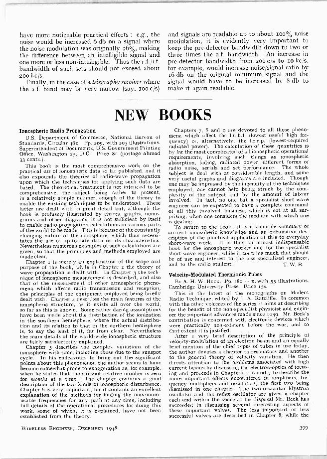
ALI I I Ai IILI C Jil

have more noticeable practical effects : e.g., the noise would be increased 6 db on a signal where the noise modulation was originally 16%, making the difference between an intelligible signal and one more or less non -intelligible. Thus the r.f./i.f. bandwidth of such sets should not exceed about 200 kc/s.

Finally, in the case of a telegraphy receiver where the a.f. band may be very narrow (say, ioo c/s)

and signals are readable up to about l00% noise modulation, it is evidently very important to keep the pre -detector bandwidth down to two or three times the a.f. bandwidth. An increase in pre -detector bandwidth from 200 c/s to Io kc/s, for example, would increase noise/signal ratio by i6 db on the original minimum signal and the signal would have to be increased by 8 db to make it again readable.

NEW BOOKS Ionospheric Radio Propagation

U.S. Department of Commerce, National Bureau of Standards, Circular 462. Pp. 209, with 205 illustrations. Superintendent of Documents, U.S. Government Printing Office, Washington 25, D.C. Price $1 (postage abroad 33 cents.).

This book is the most comprehensive work on the practical use of ionospheric data so far published, and it also expounds the theories of radio -wave propagation upon which the techniques for applying such data are based. The theoretical treatment is not intended to be comprehensive, the object being rather to present, in a relatively simple manner, enough of the theory to enable the ensuing techniques to be understood. These latter are dealt with in great detail but, although the book is profusely illustrated by charts, graphs, nomo- grams and other diagrams, it is not sufficient by itself to enable radio -propagation calculations in various parts of the world to be made. This is because of the constantly changing nature of the ionosphere, which thus necessi- tates the use of up-to-date data on its characteristics. Nevertheless numerous examples of such calculations are given, so that the principles and methods employed are made clear.

Chapter 1 is merely an explanation of the scope and purpose of the book, while in Chapter 2 the theory of wave propagation is dealt with. In Chapter 3 the technique of ionospheric measurement is described, and also that of the measurement of other atmospheric phenomena which affects radio transmission and reception, the principles of the equipment employed being briefly dealt with. Chapter 4 describes the main features of the ionospheric structure, as it exists all over the world, so far as this is known. Some rather daring assumptions have been made about the distribution of the ionization in the southern hemisphere, where the actual distribution and its relation to that in the northern hemisphere is, to say the least of it, far from clear. Nevertheless the main details of the world-wide ionospheric structure are fairly satisfactorily explained.

Chapter 5 describes the complex variations of the ionosphere with time, including those due to the sunspot cycle. In his endeavours to bring out the significant points about this phenomenon the author seems to have become somewhat prone to exaggeration as, for example, when he states that the sunspot relative number is zero for months at a time. The chapter contains a good description of the two kinds of ionospheric disturbance. Chapter 6 is very important, for it contains an excellent explanation of the methods for finding the maximum - usable frequencies for any path at any time, including full details of the operational procedures for doing this work, some of which, it is explained, have not been established from the theory.


Chapters 7, 8 and 9 are devoted to all those phenomena which affect the 1.u.h.f. (lowest useful high frequency) or, alternatively, the I.r.r.p. (lowest -required radiated power). The calculation of these quantities is by far the most complicated of all ionospheric operational requirements, involving such things as ionospheric absorption, fading, radiated power, different forms of radio noise, aerials and set performance. The whole subject is deal with at considerable length, and some very useful graphs and diagrams are included. Though one may be impressed by the ingenuity of the techniques employed, one cannot help being struck by the com- plexity of the subject and by the amount of labour involved. In fact, no one but a specialist short-wave engineer can be expected to have a complete command of all this involved business, which is not at all sur- prising, when one considers the medium with which one is dealing.

To return to the book-it is a valuable summary of current ionospheric knowledge and an exhaustive description of the practical application of this to everyday short-wave work. It is thus an almost indispensable book for the ionospheric worker and for the specialist short-wave engineer, while it contains much that should be of use and interest to the less specialized engineer, and to the radio student. T. W. B.

Velocity -Modulated Thermionic Tubes By A. H. W. BECK. Pp. 18o -}- x, with 55 illustrations.

Cambridge University Press. Price 15s.

This is the latest of the monographs on Modern Radio Technique, edited by J. A. Ratcliffe. In common with the other volumes of the series, it aims at describing for the benefit of the non -specialist physicist and engineer the important advances made since 1939. Mr. Beck's contribution is concerned with electronic devices which were practically non-existent before the war, and to that extent it is justified.

After a very brief description of the principle of velocity -modulation of an electron beam and an equally brief mention of the chief types of tubes in use today, the author devotes a chapter to resonators and another to the general theory of velocity variation. He then directs attention to the problems associated with high current beams by discussing the electron -optics of focus- ing and proceeds in Chapters 5, 6 and 7 to describe the more important effects encountered in amplifiers, frequency multipliers and oscillators, the first two being dismissed in one chapter. The two -resonator klystron oscillator and the reflex oscillator are given a chapter each and within the space at his disposal Mr. Beck has succeeded in discussing several interesting aspects of these important valves. The less important or less successful valves are described in Chapter 8, while the

399

of the pulse we have a closed conduction current. Also, with the shortest pulses used at present with cathode-ray tubes, the pulse duration is much greater than the transit time of an electron in the tube. Again, we would have what is practically a direct current flowing through the tube, and round the circuit, during the pulse.

Fig. 4 shows a charge Q moving along the axis of a toroidal coil, so that part of the magnetic field of Q links the turns of the toroid. As the charge approaches, an e.m.f. is induced in the coil in the direction shown. Suppose the circuit is closed ; then the induced current as it grows will induce an electric field along the axis of the toroid in the direction of motion of Q. That is, the effect is to accelerate the charge, and not to retard it.

As soon as the current dI passes its maximum and

commences to fall, the induced force on Q reverses and the charge will then be retarded. Where does the energy come from, when

Q+ the current is increasing, to accelerate the charge, and also supply the ohmic loss in the coil ? According to Maxwell's theory it

Fig. 4 n comes from the magnetic field of the moving charge. There is an exact balance of energy but, and I think

this point is significant, the whole hypothesis seems to depend on the real existence of a store of magnetic energy localized in the space surrounding the charge, and many scientists ( Jeans in particular) have told us that this idea is not really tenable in the light of modern physical knowledge. If, then, we must abandon the idea of stored energy in the aether (as distinct from radiation), there does appear to be an anomaly in the conservation of energy in this problem.

There is also trouble in the inequality of action and reaction. Suppose, in Fig. 4, that a constant current I is maintained in the toroid by an external source. Then as Q moves along the axis of the coil it experiences no magnetic or induced force whatever, whereas it exerts a magnetic force of repulsion on the toroid.

The explanation by Maxwell's theory is that the reaction to the force on the toroid is borne by the aether, but again I understand that no modern physicist of repute really believes this at the present day. Thus I conclude that the problem is well worth further study. The theory of Ritz has possibilities, but fails in this very problem because it gives no reaction on the toroid, and a reaction is certainly required in the case in which a short-circuited toroid moves relatively to a stationary charge.

E. G. CULLWICK Dept. of Defence, Ottawa.

dt

Ring -Aerial Systems

Sir,-I wish to correct an error in my paper " Ring Aerial Systems : Minimum Number of Radiators Required," which appeared in the October 1948 issue of Wireless Engineer.

In the second paragraph on page 311, reference is made to the directions in which polar diagram maxima and minima occur. These are in error by 90°, due to the fact that, in Fig. 3, OC is at right angles to the reference direction, namely the projection of OP in the horizontal plane.

402

The last sentence of this paragraph should, therefore, read as follows

" If s exceeds n by an even number, there will be polar diagram maxima at right angles to the direction of individual aerials, the right angle being measured in the direction of phase rotation ; if s exceeds n by an odd number, there will be corresponding polar diagram minima in these directions."

British Broadcasting Corporation, Hinksey Hill, Oxford.

H. PAGE.

Simplified Magnetic Amplifier

SIR,-I would like to refer to D. A. Bell's letter on magnetic amplifiers which appeared in your September issue. In Fig. 3 of this letter is shown a circuit in which the standing current for zero signal is balanced in the output by using two iron cores only, in a parallel resonant circuit. This circuit goes out of resonance when a d.c. input signal is applied and so gives an alternating current into the load.

I would like to draw your attention to another type of simplified magnetic amplifier circuit which gives perfect balance of output current for zero signal input, proportionality between output and input, as well as discrimination in the response to inputs of different polarity.' The arrangement is shown in the accompanying diagram, and d.c. magnetization in the two arms (I) and (2) of the magnetic circuit is produced by the rectifier D

connected to the main a.c. winding. In the absence of any input signal, there is no current

in the load because of the symmetry of the magnetic circuits and of the opposing halves of the output windings.

LOAD

D

o

o INPUT

o

When a d.c. input signal is applied, this reduces the d.c. magnetization in one arm of the magnetic circuit and increases it in the other. This causes the e.m.f. in one half of the output winding to increase and that in the other to decrease thus giving a differential alternating current in the load. When this is rectified, it is seen that its effect is to aid the cause for an input of one polarity and to oppose it for an input of the opposite, and this gives discrimination between the two cases.

The choke L prevents the alternating current in the output from being induced into the input.

M. MARINESCU. Electrical Communication Laboratory,

Polytechnic School, Bucarest.

' "Amplificateurs Magnétiques," M. Marinescu, Acad. Roumaine, Bull. de la Section Scientifique, T.XXVIII, No. 3, 1945.


WIRELESS PATENTS A Summary of Recently Accepted Specifications

The following abstracts are prepared, with the permission of the Controller of H.M. Stationary Office, from Specifications obtainable at the Patent Office, 25, Southampton Buildings, London, W.C.2, price 2/- each.

DIRECTIONAL AND NAVIGATIONAL SYSTEMS

595 832.-Radiolocation system in which the exploring beam is automatically swung over a given terrain by cyclically varying the frequency fed to an aerial array.

Marconi's W.T. Co. Ltd. (assignees of I. Wolff). Convention date (U.S.A.) 23rd April, 1943.

595 837 -Directional aerial comprising a hollow horizontal boom, pivoted centrally, and carrying at each end a transverse loop which is suitably tilted to offset undesired coupling effects.

A. H. Stevens (communicated by United Air Lines Inc.). Application date 13th June, 1944--

595 893.-Waveguide coupling and feed arrangement for a parabolic aerial designed to radiate a fan -shaped beam, particularly for airborne radiolocation sets.

Western Electric Co. Inc. Convention date (U.S.A.) 26th July, 1944.

596 314.-Radiolocation system in which the scanning beam describes a cone in space, and provision is made to ensure the accurate tracking of a moving target.

Western Electriv Co. Inc. Convention date (U.S.A.) 24th February, 194,1.-

596 391 -Aerial array in which parasitic radiation from asymmetrically -arranged elements is utilized to increase the sharpness of the directional pattern.

Standard Telephones and Cables Ltd. (assignees of S. B. Pickles). Convention date (U.S.A.) 15th November, 1943.

596 442. -Aerial system comprising inner and outer pairs of suitably -phased dipoles for marking out a navigational course of the overlapping -beam type.

Marconi's W.T. Co. Ltd. (assignees of G. H. Brown). Convention date (U.S.A.) 30th September, 1941.

596 447 Navigational equipment in which radiolocation is combined with gyroscopic control to indicate and correct any drifting from a set course.

Western Electric Co. Inc. Convention date (U.S.A.) 21st March, 1944.

596 479. -Feeding and screening arrangements for reducing the effect of parasitic currents in directive aerials of the Adcock type.

Standard Telephones and Cables Ltd. (assignees of H. G. Busignies). Convention date (U.S.A.) 2nd June, 1942.

596 515.-Radiolocation receiver with an input circuit which is designed to discriminate against ground and other undesired echo signals of large pulse width.

S. Jefferson and K. Hopkinson. Application date 27th July, 1945-

596 611. -Group of three spaced loop aerials, one central and periodically switched, forming a directive unit which is free from polarization error.

F. Tench (communicated by Automatic Electric Labora- tories Inc.). Application date 29th June, 1945.

596 6i4. -Elevated four -loop aerial beacon for radiating two crossed figure -of -eight patterns of plane -polarized waves.

Standard Telephones and Cables Ltd. (assignees of N. Marchand). Convention date (U.S.A.) 22nd July, 1944.

596 657.-Radiolocation system of the kind in which the Doppler effect is utilized to distinguish the echo signals from a moving target, particularly on a plan - position indicator.

A. E. Bailey and E. H. Rhoderick. Application date 19th February, 1945.

596 691. -Mobile direction finder in which a true indication is secured by analysing the relation between in -phase vectors at selected points on a stationary interference pattern.

Standard Telephones and Cables Ltd. (communicated by Internationál Standard Electric Corp.). Application date 17th July, 1945.

596 804. -Direction -finding system in which a true indication is secured by opposing the separate signals received on horizontally and vertically polarized aerials.

Standard Telephones and Cables Ltd. (assignees of H. G. Busignies). Convention date (U.S.A.) 22nd January, 1943.

597 052. -Time base and potentiometer arrangement designed to increase the accuracy of short-range measurements in radiolocation.

J. W. Pletts. Application date 2nd May, 1945-

597 o94.-Radiolocation system of the kind in which the Doppler effect is utilized to distinguish the echo - signals received from fixed and moving objects, particularly on a plan -position indicator.

A. E. Bailey. Application date 9th March, 1945.

597 184. -Gate circuit controlled by a strobing voltage for selecting a given echo -signal in radiolocation equip - nient.

R. S. Webley. Application date 31st July, 1945.

597 258. -Phase -changing devices for varying the effective length of a waveguide, used say for swingnig the exploring beam in radiolocation.

E. Pickup, G. E. Bacon and P. H. T. Brook. Application date 14th July, 1945.

RECEIVING CIRCUITS AND APPARATUS (See also under Television)

595 805. -Relay arrangement for preselecting one or more of the separate items broadcast on a given wavelength, provided each item is preceded by a characteristic pulsed signal.

Electrical Components Ltd. and W. Sommer. Applica- tion date 15th June, 1945.

596 439. -Construction and application of a cavity - resonator device for automatic frequency stabilization or modulation, or for tuning -control.

" Patelhold" Patentverwertungs &c. A.G. Convention date (Switzerland) 6th November, 1943.

596 519. -Receiver comprising a pair of series -resonant circuits for detecting phase or frequency modulated signals.


,a'mum i iLA Jim Lid

Marconi's W.T. Co. Ltd. (assignees of G. L. Usselman). Convention date (U.S.A.) 28th July, 1944--

596 531. -Receiver for frequency -modulated signals in which incidental amplitude variations are applied, through gain -control, to counteract themselves.

Marconi's W.T. Co. Ltd. (assignees of N. I. Korman). Convention date (U.S.A.) 29th July, 1944.

596 617. -Receiver with ' stepped ' tuning which periodically sweeps over a wide frequency range in order to detect and locate any station operating within that range.

Standard Telephones and Cables Ltd. (assignees of A. Preisman). Convention date (U.S.A.) 7th May, 1943

TELEVISION CIRCUITS AND APPARATUS FOR TRANSMISSION AND RECEPTION

595 937. -Cathode-ray receiver for photographic and like facsimile signals.

W. G. H. Finch. Convention date (U.S.A.) 25th March, 1944-

596 of,. -Television system in which the audible components take the form of time -modulated pulses transmitted immediately after each synchronizing signal.

Standard Telephones and Cables Ltd. (assignees of T. H. Young, Junr.). Convention date (U.S.A.) 17th July, 1944. 596 o26. -Receiving circuit for time -modulated pulsed signals, particularly those forming part of a television programme.

D. I. Lawson and Pye Ltd. Application dates 14th July and 12th October, 1945.

5961o6. -Relaxation oscillator for receiving pulsed signals forming part of a combined sound -and -television waveform.

A. V. Lord, J. E. Cope and Pye Ltd. Application date 19th July, 1945-

596 394. -Television mixing circuit in which the video, audio, blanking, and synchronizing signals are separately applied to selected grids in a two -stage amplifier.

Farnsworth Television and Radio Corpn. Convention date (U.S.A.) 5th February, 1944-

596 459. -Valve circuit of the counter type arranged as a receiver for frequency -modulated signals extending over a wide range, as in television.

E. L. C. White. Application date 29th June, 1945.

597 050. -Automatic gain -control system for television, in which the correct background conditions are maintained over changing contrasts in light and shade.

Farnsworth Television and Radio Corp. Convention date (U.S.A.) Ist July, 1944.

597 234. -Television scanning system in which both the line and frame frequencies are derived from different harmonics of a primary oscillation of distorted waveform.

Farnsworth Television and Radio Corpn. Convention date (U.S.A.) 18th November, 1943.

TRANSMITTING CIRCUITS AND APPARATUS (See also under Television)

596 877. -Transmission circuit including both a linear and a non-linear amplifier for separating and regulating the carrier and sideband components of a modulated wave

Sperry Gyroscope Co. Inc. Convention date (U S.A.) 3rd May, 1944-

596 924. -Modulating device comprising two waveguide sections coupled through a balanced bridge and a pair of gratings for rotating the plane of polarization.

Western Electric Co. Inc. Convention date (U.S.A.) 16th June, 1944.

597 240. -Forming an offset junction or coupling between two rectangular waveguides through an intermediate guide section of circular cross-section.

J. B. Warren and W. D. Allen, Application date 19th April, 1945.

597 251. -Shaped block of dielectric designed, when placed inside a waveguide, to produce a desired change or transformation in the mode of wave propagation.

W. D. Allen. Application date loth June, 1945

SIGNALLING SYSTEMS OF DISTINCTIVE TYPE

595 421. -Signalling system in which keying is effected by shifting the carrier from one fixed frequency to another, and in which both frequencies are positively or directly utilized in reception.

Marconi's W.T. Co. Ltd. (assignees of G. L. Usselman). Convention date (U.S.A.) iith February, 1944.

595 624.-Multivibrator circuit for generating trains of pulses, and means for modulating their width in accord- ance with an applied signal -voltage.

Marconi's W.T. Co. Ltd. (assignees of W. A. Miller). Convention date (U.S.A.) 5th July, 1944--

595 894. -Receiving circuit for time -modulated pulsed signals in which frequency division is utilized to increase the signal-to-noise ratio.

Standard Telephones and Cables Ltd. (assignees of N. H. Young, Junr.). Convention date (U.S.A.) 6th January, 1944.

596 o51. -Multi -channel signalling system utilizing pulses modulated in time to convey one message and pulses modulated in amplitude to convey other intelli- gence.

Standard Telephones and Cables Ltd. (assignees of D. D. Grieg). Convention date (U.S.A.) 19th May, 1944.

596 o52. -Pulsed signalling -system in which a gas -filled discharge tube, having a predetermined striking - potential, serves both as generator and modulator.

Standard Telephones and Cables Ltd. (assignees of L. A. de Rosa). Convention date (U.S.A.) 17th July, 1944 .

SUBSIDIARY APPARATUS AND MATERIALS

594 431. -Wave -filter network or transmission -line for wide or narrow frequency -ranges, and for use as a phase -shifter, attenuation -equalizer, and modulator.

Telephone Manufacturing Co., Ltd., and W. Saraga. Application date 29th May, 1945.

595 073. -Scanning -control for a c.r. tube, in .which a full -wave rectifier produces a train of positive pulses as an intermediate step between a sinusoidal source and a saw-toothed wave.

Marconi's W.T. Co. Ltd. (assignees of E. H. Schoenfeld). Convention date (U.S.A.) 28th July, 1943- 595 200. -Stabilized harmonic generator comprising a grid -controlled discharge tube having a time -constant circuit for controlling the anode voltage.

Marconi's W.T. Co. Ltd. (assignees of G. L. Usselman). Convention date (U.S.A.) 15th May, 1943.

595 487. -Stroboscopic device for use with a cathode- ray tube for indicating or measuring and monitoring frequencies.

A. Graves, T. J. Dawes and Alltools Ltd. Application date 5th July, 1945.

404 WIRELESS ENGINEER, DECEMBER 1948