Winter North Atlantic Oscillation Hindcast Skill: 1900–2001

Winter North Atlantic Oscillation Hindcast Skill: 1900–2001

CHRISTOPHER G. FLETCHER* AND MARK A. SAUNDERS

Department of Space and Climate Physics, Benfield Hazard Research Centre, University College London, Surrey, United Kingdom

(Manuscript received 7 January 2005, in final form 13 March 2006)

ABSTRACT

Recent proposed seasonal hindcast skill estimates for the winter North Atlantic Oscillation (NAO) arederived from different lagged predictors, NAO indices, skill assessment periods, and skill validation meth-odologies. This creates confusion concerning what is the best-lagged predictor of the winter NAO. Torectify this situation, a standardized comparison of NAO cross-validated hindcast skill is performed againstthree NAO indices over three extended periods (1900–2001, 1950–2001, and 1972–2001). The lagged pre-dictors comprise four previously published predictors involving anomalies in North Atlantic sea surfacetemperature (SST), Northern Hemisphere (NH) snow cover, and an additional predictor, an index of NHsubpolar summer air temperature (TSP). Significant ( p � 0.05) NAO hindcast skill is found with May SST1900–2001, summer/autumn SST 1950–2001, and warm season snow cover 1972–2001. However, the highestand most significant hindcast skill for all periods and all NAO indices is achieved with TSP. Hindcast skillis nonstationary using all predictors and is highest during 1972–2001 with a TSP correlation skill of 0.59 anda mean-squared skill score of 35%. Observational evidence is presented to support a dynamical linkbetween summer TSP and the winter NAO. Summer TSP is associated with a contemporaneous midlatitudezonal wind anomaly. This leads a pattern of North Atlantic SST that persists through autumn. Autumn SSTsmay force a direct thermal NAO response or initiate a response via a third variable. These findings suggestthat the NH subpolar regions may provide additional winter NAO lagged predictability alongside themidlatitudes and the Tropics.

1. Introduction

The North Atlantic Oscillation (NAO) is the domi-nant mode of boreal winter climate variability over theNorth Atlantic (Walker and Bliss 1932; Barnston andLivezey 1987). The NAO is strongly linked to patternsof winter temperature, precipitation, and storminessover the whole North Atlantic sector (Hurrell 1995;Trigo et al. 2002). Accurate and timely forecasts of thewinter NAO are therefore an important challenge forseasonal forecasters and increasing research is focusingon improving the quality and lead time of NAO pre-dictions.

Empirical winter NAO forecast models are formu-

lated using observations of slowly varying boundaryvariables such as sea surface temperature (SST) andsnow cover. The persistence of these boundary condi-tions and their forcing of the atmosphere can makeseasonal atmospheric conditions predictable at a latertime (Goddard et al. 2001). Winter NAO forecasts havealso recently been produced using general circulationmodels (GCMs; e.g., Palmer et al. 2004). However, onlyone or two GCMs produce statistically significant fore-cast skill at levels comparable to empirical models, andonly when assessed over a relatively short time period(1980–2001).

Recent empirical studies have uncovered links be-tween North Atlantic SST anomalies in the precedinglate spring/summer/autumn and the upcoming winterNAO. Rodwell and Folland (2002) highlighted a pat-tern of May North Atlantic SST that is related signifi-cantly to the upcoming winter mean 500-hPa geopoten-tial height field, achieving a hindcast correlation skill(rs) of rs � 0.45 for the period 1948–97. Saunders andQian (2002) found that two modes of late summer/earlyautumn North Atlantic SST variability 1950–2001 wereskillful in predicting a range of upcoming winter NAO

* Current affiliation: Atmospheric Physics Group, Departmentof Physics, University of Toronto, Toronto, Ontario, Canada.

Corresponding author address: Christopher Fletcher, Atmo-spheric Physics Group, Department of Physics, University of To-ronto, 60 St. George St., Toronto, ON M5S 1A7, Canada.E-mail: [email protected]

5762 J O U R N A L O F C L I M A T E VOLUME 19

© 2006 American Meteorological Society

JCLI3949

indices with rs between rs � 0.47 and rs � 0.63. A horse-shoelike North Atlantic summer SST pattern has alsobeen shown to explain up to 16% of the early winteratmospheric variance 1958–97 (Drévillon et al. 2001;Czaja and Frankignoul 2002; Cassou et al. 2004).

Another lagged NAO predictor is the monthly meanareal extent of snow cover over different regions of theNorthern Hemisphere (NH). Reliable satellite observa-tions of snow cover are available only since 1972(Robinson et al. 1993). Thus, the role of anomaloussnow cover in influencing atmospheric circulation andclimate has received less attention than that of SSTanomalies. Saunders et al. (2003) used NH snow coverto predict a range of NAO indices and found that theJune–July mean produced the most significant hindcastskill with rs � 0.61 for 1972–2001. A significant corre-lation of r � �0.56 is highlighted by Bojariu andGimeno (2003) between April and October mean Eur-asian (EU) snow cover and the upcoming winter NAOindex 1973–98. These studies suggest a recent signifi-cant link between NH climate in the warm season andthat in the upcoming winter. Cohen and Entekhabi(1999) highlighted the significant relationship betweenEU snow cover during fall and the upcoming winterArctic Oscillation (AO) index. However, these linkswere not significant when assessed against the NAOindex.

The above discussion highlights the current confusingsituation in the literature where several authors claimto have uncovered significant predictive links and skillfor the winter NAO using different prior climatic pre-dictors. Furthermore, these authors all reference theselinks and skill to different NAO indices and/or employdifferent predictand time periods and/or use differentskill assessment methodologies and measures. In thisstudy we compare the most skillful recent empiricalhindcast models using the same hindcast procedure forall predictors. This provides a standardized platform onwhich to evaluate and compare the skill arising fromthe chosen NAO predictors. Hindcasts are made forthree different winter NAO indices over three ex-tended time periods out to 100 yr and skill is assessedusing two skill measures. Where possible, hindcast skillsensitivity to choice of predictor observational datasetis also examined by using two datasets for each analysis.These methods will allow us to quantify which of thelagged predictors drawn from the recent literature pro-vides the best hindcast skill for the upcoming winterNAO.

The paper is structured as follows. Section 2 outlinesthe chosen assessment periods, predictand NAO indi-ces, predictors and the different observational datasetsused to compute them. Here we also describe our hind-

cast procedure and the method for evaluating hindcastskill and its statistical significance. Results from thehindcast comparison are presented in section 3, wherestationarity of the predictive relationships is also dis-cussed. Section 4 provides an interpretation of the keyfindings and examines the physical mechanisms linkingthe most skillful lagged predictor to the winter NAO.Section 5 discusses the implications of our work forseasonal forecasting in general and a summary and con-clusions are presented in section 6.

2. Data and methods

Henceforth, “winter” denotes the three-month De-cember–February (DJF) seasonal mean and “winterNAO” will be referred to as NAODJF. Previous studiesof NAODJF hindcast skill have examined data since1950. Here, we assess hindcast skill, where possible,over the entire twentieth century. Specifically, NAODJF

hindcast skill is assessed for the three periods 1900–2001, 1950–2001, and 1972–2001, with the 1972–2001period corresponding to the interval of reliable satellitesnow cover data (Robinson et al. 1993). These threeassessment periods also allow the stationarity inNAODJF hindcast skill to be examined.

Figure 1 shows the time series of the three NAODJF

indices employed as predictands in this study. The firstindex is the standardized difference in mean sea levelpressure (MSLP) between Reykjavik, Iceland, andGibraltar maintained by the Climatic Research Unit(CRU) at the University of East Anglia (henceforth theCRU NAODJF index; Jones et al. 1997). The second isdefined as the standardized MSLP difference betweenStykkisholmur, Iceland, and Ponta Delgada, Azores,provided by the National Center for Atmospheric Re-search (NCAR) Climate Analysis Section (henceforththe Hurrell NAODJF index). The third index is the timeseries of 500-hPa North Atlantic geopotential heightcoefficients from a singular value decomposition (SVD)analysis with May North Atlantic SST (henceforth theZ500DJF index; Rodwell and Folland 2002).

a. Previously published NAODJF predictors

The four previously published NAODJF predictorsexamined in this study are shown in Table 1 and aretaken from results published since 2001. They were se-lected for comparison because they are believed to en-compass the highest currently observed seasonal pre-dictive skill for the winter NAO.

The first NAODJF predictor [henceforth the May SST(SVD)] is the time series of May North Atlantic (10°–80°N) SST derived from an SVD analysis with DJF

15 NOVEMBER 2006 F L E T C H E R A N D S A U N D E R S 5763

mean 500-hPa geopotential height over the North At-lantic sector (Rodwell and Folland 2002). The SVDprocedure was performed in “cross-validated” mode,with the resulting SST expansion coefficients called the“predicted” NAO series and the corresponding geopo-tential height coefficients the “observed” NAO series.The correlation skill was taken as the Pearson correla-tion between these two time series.

Our implementation of the SVD analysis differs fromthat employed by Rodwell and Folland (2002). First, inaccordance with other analyses in this study, we employa 5-yr block elimination to the SVD procedure. Thismeans that we remove each year in turn and addition-ally 2 yr on either side. Second, we remove sea ice fromthe SST fields prior to performing the SVD (sea ice wasretained in the original analysis). Third, we employ dif-ferent data periods. Fourth, we compute skill from adetrended data analysis. These differences in imple-mentation mean that our results are expected to differ

from those of Rodwell and Folland (2002). However, asa preliminary check, we first reproduced the cross-validated hindcast correlation skill (rs � 0.45) usingtheir original implementation. This predictor maxi-mizes covariance with the Z500DJF index; however, wealso assess its hindcast skill against all NAO indices.

The second predictor is the second principal compo-nent (PC2) of the June–October (JJASO) mean NorthAtlantic (0°–65°N) SST. This is slightly the stronger oftwo lagged JJASO SST predictive modes employed bySaunders and Qian (2002). The PC2 loading pattern(see their Fig. 1a) features a ring of SST anomaliesaround an opposite-signed center off southeast New-foundland.

The third and fourth predictors employ the monthlymean areal extent of snow cover, with observationsconsidered reliable since 1972. The third predictor issnow cover over Eurasia for the period April–October(A–O; Bojariu and Gimeno 2003). The fourth predictor

FIG. 1. Temporal evolution of the (a) CRU, (b) Hurrell, and (c) Z500DJF indices 1900–2001 in standardized units.The Z500DJF index is computed using HadSLP data 1900–98. Pearson correlation coefficients between the indices(1900–2001): (a) and (b) � 0.88, (a) and (c) � 0.88, (b) and (c) � 0.85.

TABLE 1. Published NAODJF lagged predictors examined in this paper.

Lagged predictorAssessment

periodLead time(months) Domain area NAODJF index Reference

May SST (SVD) 1948–98 6 10°–80°N, 90°W–40°E Z500DJF Rodwell and Folland (2002)JJASO SST (PC2) 1950–2001 1 0°–65°N, 100°W–0° CRU/CPC*/PC1 Saunders and Qian (2002)AMJJASO EU snow cover 1972–2000 1 n/a Hurrell (1995) Bojariu and Gimeno (2003)JJ NH snow cover 1972–2002 4 n/a CRU/CPC/PC1 Saunders et al. (2003)

* U.S. Climate Prediction Center index.


is the June–July (JJ) mean snow cover for the entireNH (Saunders et al. 2003).

b. An additional NAODJF predictor

Alongside the four previously published predictorsoutlined above, we also compare an index of JJ meanNH subpolar (60°–70°N) 2-m air temperature. Thisindex and its link to the upcoming winter NAO wasintroduced by Saunders et al. (2003). The index is de-fined as

TSUBPOLAR �NA � EU

2� SG, �1�

where North America (NA), Eurasia (EU), and south-ern Greenland (SG) refer to subpolar (60°–70°N) 2-mair temperatures over these areas (Fig. 2). These cen-ters correspond to where gridded JJ air temperature iscorrelated most significantly with contemporaneousNH snow cover (|r | � 0.5 1972–2001).

Gridded 2-m air temperature data back to 1900 areavailable from the CRU Air Temperature Amomaliesversion 2 (CRUTEM2) dataset (Jones and Moberg2003) for NA, EU, and SG. We therefore calculate theTSUBPOLAR index (TSP) for the period 1900–2001 and

employ it as an NAODJF predictor. The summer periodis selected because during the summer months the re-lationship peaks between the TSP index and the upcom-ing winter NAO (Saunders et al. 2003). Figure 3shows that the link is strongest in JJ using both theCRUTEM2 and the (National Centers for Environ-mental Prediction) NCEP–NCAR reanalysis data (Kal-nay et al. 1996) for the 50- and 30-yr assessment peri-ods. However, for the 100-yr period the link is signifi-cant over an extended summer period May–September(MJJAS). Therefore, we also evaluate the NAODJF

predictive skill of the longer MJJAS mean TSP.

c. Predictor datasets

The May SST (SVD) assessment back to 1900 is per-formed using MSLP data because pre-1948 geopoten-tial height data are not available. This analysis is per-formed over the shorter period 1900–98. This is theperiod of extended MSLP data available from theUnited Kingdom Met Office (UKMO) Hadley CentreSea Level Pressure (HadSLP) dataset, which is an up-date of the Met Office’s Global Mean Sea Level Pres-sure (GMSLP2.1f; Basnett and Parker 1997). Geopo-tential heights at 500 hPa (1950–2001) are taken fromthe NCEP–NCAR reanalysis (Kalnay et al. 1996). TheNH gridded surface air temperatures 1900–2001 arefrom the University of East Anglia CRUTEM2 (5° � 5°latitude–longitude grid) dataset (Jones and Moberg2003) and for the periods since 1950 are also from theNCEP–NCAR reanalysis.

Two global gridded SST datasets are employed inthis study. For the period 1900–2001, we use the MetOffice Hadley Centre Coupled Sea Ice and SST(HadISST) dataset (Rayner et al. 2003) and for theperiod 1950–2001 SSTs are also taken from NCEP–NCAR reanalysis. All SST data are interpolated onto a2.5° � 2.5° latitude–longitude grid for computationalefficiency. Snow cover data for EU and NH are satel-lite-derived estimates of monthly mean areal extent(Robinson et al. 1993).

Throughout our analysis we employ linear detrendedtime series corrected for autocorrelation to computeregressions and hindcast skill. This approach minimizesthe influence of time series trends and multiyear-to-decadal signal variability on the strength and signifi-cance of the deduced hindcast skill. The use of raw (notdetrended) time series corrected for autocorrelationgives in most cases hindcast skills that are of similarmagnitude and significance to those achieved with thedetrended data analysis. For reference, Table 2 showsthe linear trends in NAODJF and the three predictorsfor each assessment period. Over the 100-yr period thetrends are negative or close to zero. However, since

FIG. 2. The correlation pattern significance between detrendedtime series of JJ NH snow cover extent and gridded JJ 2-m airtemperature. Significances are corrected for serial correlationwith lags out to 15 yr included. Grayscale denotes where correla-tion is positive (light) or negative (dark). (After Saunders et al.2003.)


1950 all three NAODJF indices and JJ TSP exhibit posi-tive trends of �0.2–0.3 standard deviations per decade.Also shown is the percentage of NAODJF hindcast cor-relation skill that is attributable to linear trend, which iscalculated as

�SKILL � �1 �rs

r�s� � 100%, �2�

where rs is the correlation skill from the detrended dataanalysis and rs is the correlation skill obtained usingraw (not detrended) time series. For the 1900–2001 pe-riod the inclusion of trends decreases the hindcast skillby 4%–200%; for the 1950–2001 period it increases skillby 14%–46% (for May SST there is a 30%–50% de-crease); for 1972–2001 it decreases skill by 0%–40%(for May SST there is a 40%–60% increase). Thesedifferences reflect the decadal and longer time-scale

variability in the NAODJF and predictor indices (seealso section 3b).

d. Hindcast methodology

The predictive skill of the selected NAODJF predic-tors is computed for each assessment period usingcross-validated (Michaelsen 1987) hindcasts with blockelimination. Except for the May SST (SVD) predictor,linear empirical models for the NAODJF index y in agiven year t using predictor x take the following form:

yt � �0 � �1xt � et, �3�

where the coefficients 0 and 1 are determined by anordinary least squares regression and et is the residual.A 5-yr block elimination is employed, which means thatfor a given predictand year t, data for the years t � 2,t � 1, t, t � 1, and t � 2 are removed from the regres-sion. Furthermore, predictors derived from principal

FIG. 3. Magnitude, sign, and significance of linear correlation between the lagged bimonthly TSP temperature index and the upcomingCRU NAODJF index. (left) Correlations for the CRUTEM2 TSP index and (right) NCEP–NCAR data. Dark lines denote the corre-lation magnitude and sign. Faint lines denote the correlation 5% significance level corrected for serial correlation.

TABLE 2. Linear trend in NAODJF indices and predictors in standardized units per decade (columns 3, 4, 6, and 8). The percentageof NAODJF hindcast correlation skill attributable to linear trend (�Skill, columns 5, 7, and 9). See text for calculation of �Skill.

Assessmentperiod NAODJF index

NAODJF

trend

May SST (SVD) JJASO SST (PC2) JJ TSP

Trend �Skill Trend �Skill Trend �Skill

1900–2001 CRU NAODJF �0.07 0.03 �4 0.07 �111 0.12 �200Hurrell NAODJF �0.02 — �4 — �24 — �26Z500DJF �0.05 — �4 — �70 — �100

1950–2001 CRU NAODJF 0.21 0.33 �40 �0.15 19 0.31 14Hurrell NAODJF 0.21 — �29 — 23 — 21Z500DJF 0.27 — �50 — 46 — 19

1972–2001 CRU NAODJF 0.23 �0.52 41 0.18 �40 0.29 �2Hurrell NAODJF 0.13 — 40 — �17 — �4Z500DJF 0.23 — 60 — �7 — 0


components (PCs) are also subjected to block elimina-tion in their formulation. For each predictor, a timeseries of hindcasted NAODJF values is calculated whoseskill is verified against the corresponding observedNAODJF series.

e. Skill assessment

In validating the hindcast skill from each predictor,we employ the Pearson product-moment correlationskill (rs) and the mean-squared skill score (MSSS)against a simple prediction of climatology. Climatologyin this study is the long-term mean for each assessmentperiod because the NAODJF is known to be nonstation-ary during the twentieth century (Hurrell and van Loon1997). This nonstationarity means that no single 30-yrclimatology period is representative of the twentiethcentury as a whole. However, our conclusions are notsensitive to the choice of climatology.

The statistical significance of each skill value is esti-mated using a randomized resampling method (Manly1997). Our null hypothesis (H0) is that there is no linkbetween a given predictor and the NAODJF and there-fore any observed skill is achieved by random chance.The observed and hindcast NAODJF time series areboth randomly shuffled (with replacement) to createtwo new synthetic time series drawn from the samepopulations as the original time series. The length ofthe two synthetic time series is reduced to equal the“effective” number of degrees of freedom between theoriginal time series, taking into account serial correla-tion (Davis 1976). Skill values are calculated for the tworandomized time series and this shuffling/resamplingprocess is repeated in Monte Carlo fashion 25 000times. The statistical significance is determined by thenumber of cases where the skill value from the randomdata exceeds the original observed skill value. The apriori threshold of statistical significance is set at 0.05,which represents the probability that H0 is incorrectlyrejected. Our test is one tailed as only positive values ofrs and MSSS will lead to a rejection of H0 (Wilks 1995).

3. NAO hindcast skill

a. Comparison by assessment period

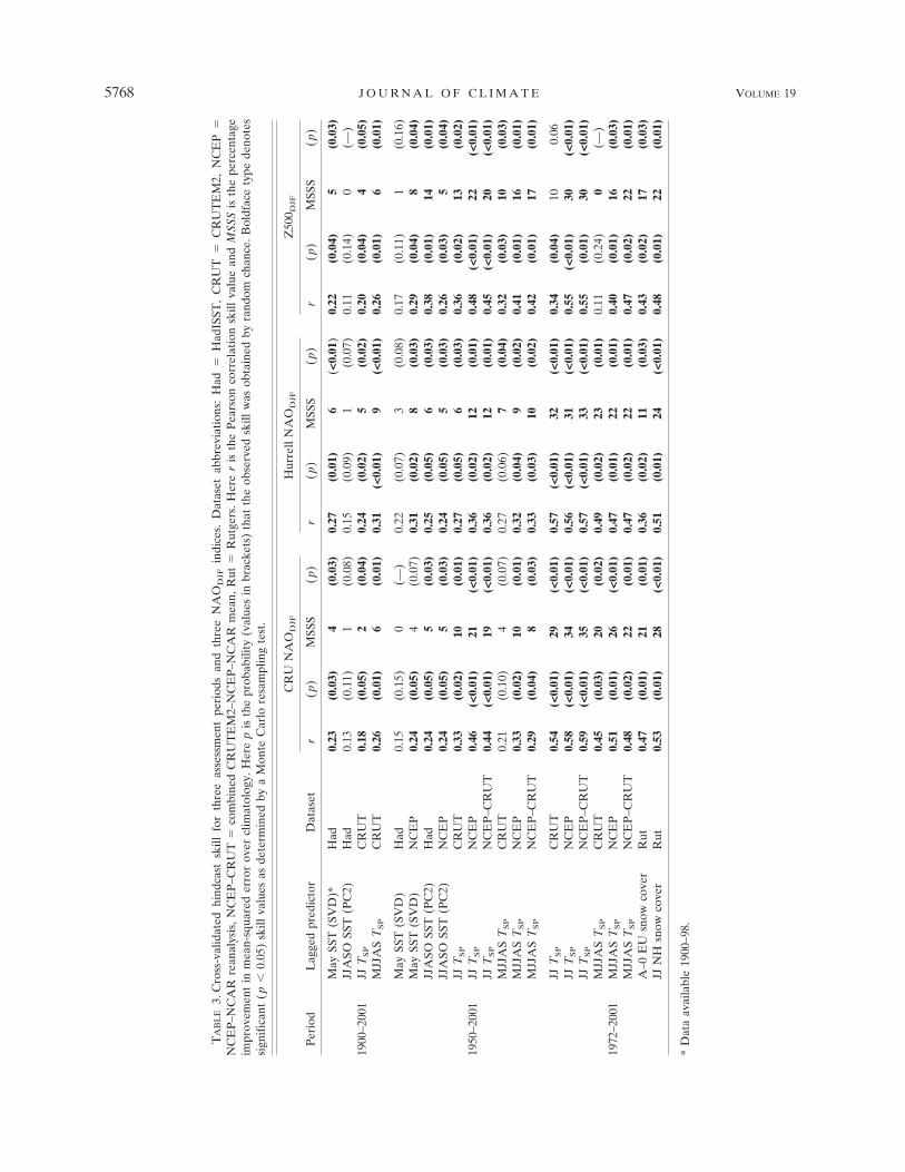
Table 3 shows the NAODJF cross-validated hindcastskill (and significance) for each predictor against thethree NAODJF indices over all three assessment timeperiods. For the 100-yr period, significant hindcastskill is found using May SST (SVD) and both TSP

index predictors. The long summer [May–September(MJJAS)] mean produces the highest skill (a 6%–9%improvement over a prediction of climatology) and the

JJ mean results in a 2%–5% improvement. Values ofrs range from 0.26 to 0.31 for MJJAS, which represent7%–10% of NAODJF variance over 100 yr. The JJASOSST (PC2) predictors shows positive, but not signifi-cant, skill over this period. There is little variability inpredictive skill by predictor with NAO index.

For the 50-yr assessment period, statistically signifi-cant skill is achieved using the two SST predictors andboth TSP indices. However, the May SST (SVD) pre-dictor is significant only when calculated using NCEP–NCAR SST and not using HadISST. In contrast tothe 1900–2001 period, it is the JJ TSP rather than theMJJAS TSP that is most skillful for all three NAO in-dices. The former has maximum rs � 0.48 and MSSS �22%, whereas for the MJJAS index the maximum skillvalues are rs � 0.41 and MSSS � 16%. The CRUTEM2TSP indices show skill 20%–30% lower in this assess-ment period than the NCEP–NCAR TSP indices. Anensemble mean TSP index is calculated using the meanof the CRUTEM2 and NCEP–NCAR data. This pro-duces skill levels close to those achieved using NCEP–NCAR alone. In terms of skill variation with NAODJF

index, all predictors except May SST (SVD) performbest against Z500DJF for this assessment period.

Highest hindcast skill in the 1972–2001 period isachieved using the JJ TSP index and the two snow coverpredictors. The JJ TSP index shows the highest skillvalues (maximum rs � 0.59 and MSSS � 35%) this skillshowing little sensitivity to NAODJF index or choice oftemperature dataset. The JJ NH index is slightly themore skillful of the two snow cover predictors (maxi-mum rs � 0.53 and MSSS � 28%) against all threeNAODJF indices. As in the 50-yr assessment, the linkbetween TSP and the NAODJF indices is strongest forthe JJ period rather than for the long summer (MJJAS)period. The combined CRUTEM2–NCEP–NCARmean JJ TSP index shows skill slightly higher than thatachieved with each single dataset JJ TSP index. ForMJJAS TSP, skill is similar to that achieved using singledataset indices for CRU and Hurrell NAODJF buthigher against Z500DJF. The A–O mean Eurasian snowcover produces significant skill against all three NAOindices, although it displays sensitivity to NAODJF in-dex. Neither of the SST-based predictors produce sig-nificant skill for the 30-yr assessment period (notshown).

b. Stationarity

The differences observed in NAODJF predictive skillfrom summer TSP between the 1900–2001 assessmentperiod and the 1972–2001 period suggest that the rela-tionship between TSP and the NAODJF is nonstationary.


TA

BL

E3.

Cro

ss-v

alid

ated

hind

cast

skill

for

thre

eas

sess

men

tpe

riod

san

dth

ree

NA

OD

JFin

dice

s.D

atas

etab

brev

iati

ons:

Had

�H

adIS

ST,

CR

UT

�C

RU

TE

M2,

NC

EP

�N

CE

P–N

CA

Rre

anal

ysis

,N

CE

P–C

RU

T�

com

bine

dC

RU

TE

M2–

NC

EP

–NC

AR

mea

n,R

ut�

Rut

gers

.H

ere

ris

the

Pea

rson

corr

elat

ion

skill

valu

ean

dM

SSS

isth

epe

rcen

tage

impr

ovem

ent

inm

ean-

squa

red

erro

rov

ercl

imat

olog

y.H

ere

pis

the

prob

abili

ty(v

alue

sin

brac

kets

)th

atth

eob

serv

edsk

illw

asob

tain

edby

rand

omch

ance

.Bol

dfac

ety

pede

note

ssi

gnif

ican

t(p

�0.

05)

skill

valu

esas

dete

rmin

edby

aM

onte

Car

lore

sam

plin

gte

st.

Per

iod

Lag

ged

pred

icto

rD

atas

et

CR

UN

AO

DJF

Hur

rell

NA

OD

JFZ

500 D

JF

r(p

)M

SSS

(p)

r(p

)M

SSS

(p)

r(p

)M

SSS

(p)

May

SST

(SV

D)*

Had

0.23

(0.0

3)4

(0.0

3)0.

27(0

.01)

6(<

0.01

)0.

22(0

.04)

5(0

.03)

JJA

SOSS

T(P

C2)

Had

0.13

(0.1

1)1

(0.0

8)0.

15(0

.09)

1(0

.07)

0.11

(0.1

4)0

(—)

1900

–200

1JJ

TS

PC

RU

T0.

18(0

.05)

2(0

.04)

0.24

(0.0

2)5

(0.0

2)0.

20(0

.04)

4(0

.05)

MJJ

AS

TS

PC

RU

T0.

26(0

.01)

6(0

.01)

0.31

(<0.

01)

9(<

0.01

)0.

26(0

.01)

6(0

.01)

May

SST

(SV

D)

Had

0.15

(0.1

5)0

( —)

0.22

(0.0

7)3

(0.0

8)0.

17(0

.11)

1(0

.16)

May

SST

(SV

D)

NC

EP

0.24

(0.0

5)4

(0.0

7)0.

31(0

.02)

8(0

.03)

0.29

(0.0

4)8

(0.0

4)JJ

ASO

SST

(PC

2)H

ad0.

24(0

.05)

5(0

.03)

0.25

(0.0

5)6

(0.0

3)0.

38(0

.01)

14(0

.01)

JJA

SOSS

T(P

C2)

NC

EP

0.24

(0.0

5)5

(0.0

3)0.

24(0

.05)

5(0

.03)

0.26

(0.0

3)5

(0.0

4)JJ

TS

PC

RU

T0.

33(0

.02)

10(0

.01)

0.27

(0.0

5)6

(0.0

3)0.

36(0

.02)

13(0

.02)

1950

–200

1JJ

TS

PN

CE

P0.

46(<

0.01

)21

(<0.

01)

0.36

(0.0

2)12

(0.0

1)0.

48(<

0.01

)22

(<0.

01)

JJT

SP

NC

EP

–CR

UT

0.44

(<0.

01)

19(<

0.01

)0.

36(0

.02)

12(0

.01)

0.45

(<0.

01)

20(<

0.01

)M

JJA

ST

SP

CR

UT

0.21

(0.1

0)4

(0.0

7)0.

27(0

.06)

7(0

.04)

0.32

(0.0

3)10

(0.0

3)M

JJA

ST

SP

NC

EP

0.33

(0.0

2)10

(0.0

1)0.

32(0

.04)

9(0

.02)

0.41

(0.0

1)16

(0.0

1)M

JJA

ST

SP

NC

EP

–CR

UT

0.29

(0.0

4)8

(0.0

3)0.

33(0

.03)

10(0

.02)

0.42

(0.0

1)17

(0.0

1)

JJT

SP

CR

UT

0.54

(<0.

01)

29(<

0.01

)0.

57(<

0.01

)32

(<0.

01)

0.34

(0.0

4)10

0.06

JJT

SP

NC

EP

0.58

(<0.

01)

34(<

0.01

)0.

56(<

0.01

)31

(<0.

01)

0.55

(<0.

01)

30(<

0.01

)JJ

TS

PN

CE

P– C

RU

T0.

59(<

0.01

)35

(<0.

01)

0.57

(<0.

01)

33(<

0.01

)0.

55(0

.01)

30(<

0.01

)M

JJA

ST

SP

CR

UT

0.45

(0.0

3)20

(0.0

2)0.

49(0

.02)

23(0

.01)

0.11

(0.2

4)0

(—)

1972

–200

1M

JJA

ST

SP

NC

EP

0.51

(0.0

1)26

(<0.

01)

0.47

(0.0

1)22

(0.0

1)0.

40(0

.01)

16(0

.03)

MJJ

AS

TS

PN

CE

P– C

RU

T0.

48(0

.02)

22(0

.01)

0.47

(0.0

2)22

(0.0

1)0.

47(0

.02)

22(0

.01)

A–0

EU

snow

cove

rR

ut0.

47(0

.01)

21(0

.01)

0.36

(0.0

2)11

(0.0

3)0.

43(0

.02)

17(0

.03)

JJN

Hsn

owco

ver

Rut

0.53

(0.0

1)28

(<0.

01)

0.51

(0.0

1)24

(<0.

01)

0.48

(0.0

1)22

(0.0

1)

*D

ata

avai

labl

e19

00– 9

8.


Therefore, the modest skill seen over the full 100-yrcould be drawn entirely from the 1972–2001 skillful pe-riod. To test this we first perform a rolling cross-correlation analysis for both the JJ and MJJAS TSP

indices against the CRU NAODJF index for all possible30-yr periods 1900–2001 (Fig. 4). A linear trend is re-moved from both time series prior to each correlationvalue being computed. The MJJAS TSP index peaks atthe beginning and end of the twentieth century. Bycontrast, JJ TSP is most skillful since 1950. Further in-vestigation reveals that it is the August–September pe-riod that contributes to the early 1900s peak in MJJAS(not shown). The strengthening correlations since 1950may be linked to an increase in decadal NAODJF vari-ability over the same period (Hurrell and van Loon1997).

Despite the coincidence between periods of high cor-relation and periods of strongly positive NAO index inthe early and late twentieth century (Fig. 1), the TSP

indices perform equally as well predicting either above-or below-median NAODJF events. Hindcasts usingMJJAS TSP are correctly above and below median in54% of observed above- and below-median CRUNAODJF events 1900–2001. For the period 1950–2001the JJ TSP index is correct in 64% of cases, while for1972–2001 the figure is 71%. We therefore concludethat the hindcast skill from the summer TSP indices isnonstationary and that highest positive skill is observedduring the early and late twentieth century.

c. Dataset dependence

Table 3 shows that, with the exception of May SST(SVD), the NAODJF hindcast skill exhibits little sensi-

tivity to the choice of SST or 2-m air temperaturedataset. Specifically, the JJASO SST (PC2) predictorproduces similar skill against the three NAODJF indiceswhether it is calculated using HadISST or NCEP–NCAR data 1950–2001. The largest skill sensitivity todataset is observed for the TSP indices calculated usingCRUTEM2 and NCEP–NCAR data 1950–2001. UsingCRUTEM2 data, the JJ TSP predictor explains 11% ofthe variance in the CRU NAODJF index compared with21% using NCEP–NCAR data. A possible explanationfor this difference is that, unlike the reanalysis data, theCRUTEM2 data are missing over the open ocean. TheSG TSP region is more than 50% over ocean and hasdouble the weighting of the EU and NA regions.Therefore, SG is likely to contribute the largest errorsin TSP. However, only �50% of JJ TSP skill comes fromSG, which explains why CRUTEM2 produces somepositive skill.

4. Summer TSP influence on upcoming NAODJF

a. Relationship between NAODJF lagged predictors

Quantifying the links between the different NAODJF

lagged predictors will help to explore the physical basisfor the observed lagged predictability. Cross correla-tions are performed for all predictors over the threeassessment periods (not shown). For all periods, stableand significant (p � 0.05) relationships are found be-tween the summer TSP indices and the summer/autumn(JJASO) SST (PC2) predictor. Since 1972, similar cor-relations are observed between TSP, JJASO SST (PC2)and the two warm season snow cover predictors. Theseresults imply a potential physical relationship betweenthe predictors both in time (summer–autumn) and inspace (North America, Eurasia, to the North Atlanticsector).

The NAODJF exhibits persistence from one winter tothe next (Johansson et al. 1998; Wanner et al. 2001). Wetherefore ask how much of the observed NAODJF hind-cast skill results from the influence of the previousNAODJF on the predictors? Table 4 shows that only theHurrell NAODJF 1900–2001 and Z500DJF 1950–2001have a significant (detrended) lag-1 autocorrelation.The table also shows how much hindcast predictabilitythe lag-1 NAODJF offers for predicting the May SST(SVD), JJASO SST (PC2), and JJ TSP time series. Forthe period 1900–2001, the skill values from the lag-1NAODJF are comparable to those achieved using thepredictors themselves to hindcast NAODJF (Table 3).For 1950–2001 and 1972–2001, with the exception ofMay SST (SVD), the predictors provide significantlyhigher NAODJF skill than does lag-1 NAODJF, based onall years of data. However, when composited on JJ TSP

FIG. 4. Correlation coefficients between the JJ and MJJAS TSP

indices and the upcoming CRU NAODJF index for running 30-yrwindows commencing 1900–71. Faint dashed line indicates 5%significance level corrected for serial correlation.


terciles, the lag-1 NAODJF skill for JJ TSP 1950–2001increases to rs �0.5. This suggests that when JJ TSP islarge, it responds more to the NAODJF signal from theprevious winter. However, JJ TSP is a better NAODJF

predictor than lag-1 NAODJF alone (Tables 3 and 4).This implies that the signal from the previous winterintensifies during the summer.

The results in Table 4 are similar using data withtrends included (not shown). However, some sensitivityto the choice of dataset was found for the May SST(SVD) predictor 1950–2001. Using NCEP–NCAR re-analysis SST data, the lag-1 NAODJF skill drops tors � 0.3 (p � 0.10) for both 1950–2001 and 1972–2001.The JJASO SST (PC2) predictor does not display suchsensitivity, which suggests that greater differences existfor the May SST data than for the JJASO SST fieldswhen comparing the NCEP–NCAR and HadISSTdatasets.

b. Physical basis for summer TSP influence onupcoming winter NAODJF

Seasonal atmospheric predictability in the extratrop-ics is normally assumed to be lower than for the Tropicsbecause of the presence of baroclinic instability. Thisappears to contradict the links we observe betweensummer TSP, snow cover, and the upcoming winter cli-mate. There is little persistence intrinsic to the extra-tropical atmosphere, which has a decorrelation time of�10 days. Therefore, to enable a summer–winter linkthe memory of the summer atmospheric state must per-sist in a slowly varying boundary variable that can feedback onto the atmosphere at a later time.

Following Saunders et al. (2003), we propose the fol-lowing mechanism for the influence of summer climateon that of the upcoming winter: summer (JJ) NH snowcover anomalies are negatively correlated with JJ sub-polar near-surface air temperature (T2m) over north-ern Siberia and northwest Canada and positively cor-related with JJ T2m over Southern Greenland. The re-sulting subpolar temperature pattern induces acontemporaneous atmospheric response and laggedSST response centered on the North Atlantic. The at-mospheric response is characterized by anomalies inMSLP and midlatitude zonal wind. The SST response ischaracterized by basin-scale anomalies and meridionalgradients south and east of Newfoundland. Persistenceof these SST gradients into autumn or early wintercould force either a direct thermal NAODJF response orinitiate a response via a third variable.

There is good observational evidence to support thelink between snow cover, TSP and North Atlantic SSTs.First, there is a significant correlation (p � 0.01) be-tween changes in JJ NH snow cover and JJ TSP for the

TA

BL

E4.

Lag

-1au

toco

rrel

atio

n( r

[lag

-l])

ofN

AO

DJF

indi

ces

and

cros

s-va

lidat

edsk

illfo

rpr

edic

ting

May

SST

(SV

D),

JJA

SOSS

T(P

C2)

, and

JJT

SP

from

the

prio

rN

AO

DJF

.N

otat

ions

are

the

sam

eas

inT

able

3.SS

Tda

taar

efr

omH

adIS

STan

dT

SP

data

are

from

CR

UT

EM

2.

Per

iod

Lag

ged

pred

icto

r

NA

OM

aySS

T(S

VD

)JJ

ASO

SST

(PC

2)JJ

TS

P

r[la

g-1]

(p)

r(p

)M

SSS

(p)

r(p

)M

SSS

(p)

r(p

)M

SSS

(p)

1900

–200

1C

RU

NA

OD

JF0.

13(0

.20)

0.36

(<0.

01)

12(<

0.01

)0.

00(—

)0

(—)

0.27

(0.0

1)6

(<0.

01)

Hur

rell

NA

OD

JF0.

24(0

.02)

0.38

(<0.

01)

14(<

0.01

)0.

15(0

.06)

0(—

)0.

31(<

0.01

)9

(<0.

01)

Z50

0 DJF

*0.

19(0

.06)

0.47

(<0.

01)

17(<

0.01

)0.

15(0

.54)

0(—

)0.

35(0

.03)

8(<

0.01

)19

50–2

001

CR

UN

AO

DJF

0.14

(0.3

2)0.

43(0

.01)

8(<

0.01

)0.

00(—

)0

(—)

0.00

(—)

0(—

)H

urre

llN

AO

DJF

0.24

(0.1

0)0.

50(<

0.01

)16

(�0.

01)

0.26

(0.0

3)5

(0.0

5)0.

14(0

.14)

0(—

)Z

500 D

JF0.

29(0

.05)

0.45

(0.0

2)9

(<0.

01)

0.22

(0.0

5)3

(0.0

7)0.

29(0

.02)

7(0

.03)

1972

–200

1C

RU

NA

OD

JF0.

18(0

.36)

0.60

(0.0

1)18

(<0.

01)

0.00

(—)

0(—

)0.

00(—

)0

(—)

Hur

rell

NA

OD

JF0.

27(0

.17)

0.46

0.10

)0

(—)

0.01

(0.4

0)0

(—)

0.26

(0.0

6)1

(0.0

8)Z

500 D

JF0.

18(0

.38)

0.47

(0.1

9)0

(—)

0.00

( —)

0(—

)0.

14(0

.22)

0( —

)

*U

KM

OH

adSL

Pda

ta19

00–9

8.


period 1972–2001 (Saunders et al. 2003). Second, theatmosphere adjacent to the TSP centers is significantlyperturbed during June and July. Figure 5 shows zonallyaveraged zonal wind anomalies as a function of heightabove the TSP regions and the North Atlantic in monthsbefore and during high minus low JJ TSP tercile years1950–2001. Prior to June and July the only consistentsignal for all three regions is located in the stratosphereat high latitudes during April. The signal in June andJuly over Eurasia and North America is characteristicof a strengthened polar vortex and a weakened midlati-tude jet. A corresponding teleconnected signal is seen

over the North Atlantic in June and July, which extendsfrom the surface to the lower stratosphere. A band ofsignificant anomalous westerlies is centered between50° and 60°N, with anomalous easterlies to the northand south. This highlights that during extreme years ofTSP, contemporaneous subpolar atmospheric telecon-nections are formed between northern Eurasia, north-ern Canada, and the North Atlantic during June andJuly.

Our proposed mechanism is further supported byFig. 6, which shows the hemispheric-scale anomaly pat-terns in height-averaged (925–200 hPa) zonal wind,

FIG. 5. Composite vertical cross section of zonally averaged zonal wind anomalies based on high minus lowterciles of JJ TSP index 1950–2001. Zonal averages are calculated over (a) Eurasia, 25°–70°E, (b) North America,120°–90°W, and (c) the North Atlantic, 50°–20°W. Data are dimensionless standardized anomalies. Contourinterval is 0.3 and dashed contours denote negative anomalies. Shaded areas denote significance ( p � 0.05) asdetermined by a Monte Carlo resampling test.


FIG. 6. Composite of (a) vertically averaged (925–200 hPa) North Atlantic sector zonal wind anomalies, (b) North Atlantic sectorMSLP anomalies and (c) North Atlantic SST anomalies based on high minus low terciles of JJ TSP index. Contour intervals are (a)1 m s�1, (b) 1 hPa, and (c) 0.2°C. Dashed contours denote negative anomalies and the zero contour is labeled. Shaded areas denotesignificance ( p � 0.05) as determined by a Monte Carlo resampling test.


MSLP, and SST in months before, during, and follow-ing high-minus-low JJ TSP tercile years 1950–2001. Overthe North Atlantic, the atmospheric signal strengthensin June and the SST strengthens after July. The zonalwind, MSLP, and SST signals appear causally con-nected, with the zonal wind anomalies collocated withgradients in MSLP anomalies and with SST anomalies.The atmospheric signal is prominent in June and Julybut dissipates thereafter, although it is apparent in theJJASO mean. In contrast, the SST anomaly patternstrengthens in July and persists until October. The tim-ing, lag, and spatial pattern of the SST signal is consis-tent with its forcing by the anomalous atmospheric cir-culation associated with JJ TSP. This conclusion is fur-ther supported by the significant (p � 0.05 for all timeperiods) link between JJ TSP and JJASO SST (PC2).

Figure 7 shows the mean anomalies in vertically av-eraged zonal wind, MSLP and SST for the winter sea-sons before and following high-minus-low JJ TSP ter-ciles. The situation preceding JJ TSP shows a moderatepositive NAO pattern in the zonal wind anomalies,which is further evidence that a proportion of theNAODJF predictability from JJ TSP arises through in-terannual NAO persistence (see also section 4a). How-ever, SSTs are close to climatology except near theequator, showing that the involvement of SST does notbegin until after summer. The SST pattern followingextreme JJ TSP events exhibits a strong meridional gra-dient off Newfoundland, which has persisted from sum-mer. This pattern resembles the NAO-driven North At-lantic SST tripole anomaly pattern (e.g., Czaja andFrankignoul 2002).

Next, we attempt to show whether the evolvinganomalies seen in Fig. 6 indicate a real response to JJTSP or merely represent increased climatological vari-ance in those months. This is quantified by plotting the

percentage of grid cells in each month that are locallysignificant (p � 0.05). Figure 8 shows the percentagesfor zonal wind over the region (30°–80°N, 120°W–40°E)and for SST over the region (0°–65°N, 100°W–0°). Thehorizontal lines denote approximate levels of field sig-nificance (p � 0.05) following the method of Livezeyand Chen (1983). For each month, we assume 30 spatialdegrees of freedom (DOF) in the zonal wind field and15 DOF in the SST field. These values are appropriatebecause Livezey and Chen (1983) state that hemi-spheric atmospheric fields contain �30–60 DOF. Theactual DOF in our fields may oscillate around theseestimates depending on the month. However, even witha conservative estimate for DOF of 15, the zonal windand SST maxima are both field significant.

FIG. 8. Percentage of locally significant grid cells in Fig. 6 forSST (solid line) and vertically averaged (925–200 hPa) zonal wind(dashed line) associated with high minus low terciles of JJ TSP

index. Domains used are 0°–65°N, 90°W–0° for SST and 30°–80°N, 120°W–40°E for zonal wind. Horizontal lines denote ap-proximate field significance assuming 15 spatial degrees of free-dom for SST and 30 for zonal wind.

FIG. 7. Same as in Fig. 6 except for winter (DJF) seasonal means (top) preceding and (bottom) following high minus low JJ TSP

terciles.


The zonal wind signal peaks in June and July, con-sistent with Fig. 6. The SST response develops 1 monthlater, peaking in July and August, and persisting untilOctober. The timing of the lagged SST response is con-sistent with other observational studies of atmosphere–ocean interaction (e.g., Deser and Timlin 1997). By Oc-tober, the majority of the SST signal comes from thesubtropics. The SST response decreases to December,which is associated with a more variable atmosphericpattern August–October. We therefore conclude thatthe anomalous atmospheric circulation associated withJJ TSP is leading North Atlantic SST variability with atime lag of �1 month.

5. Discussion

NAODJF hindcast skill is nonstationary during thetwentieth century, implying that the predictive relation-ships vary in time. Data quality may also contribute tothe variations in NAODJF skill. During the early part ofthe record, observations are more sparse than duringthe 1972–2001 period of highest skill. This reduction indata quality may degrade NAODJF hindcast skill andcontribute to nonstationarity.

Nonstationarity in predictive relationships may arisefrom low-frequency multiannual or decadal oscillationsin the predictor and/or predictand indices. An analysisof spectral coherency (Bloomfield 2000) was performedon the predictors and NAO indices to determine thedominant time scales of interaction. The results (notdisplayed) show that the preferred oscillatory periodfor each predictor with the NAODJF differs dependingon the assessment period. For example, the MJJAS TSP

index and CRU NAODJF index are significantly coher-ent at a period of 7 yr (1900–2001), 4 yr (1950–2001),and 8 yr (1972–2001). A further cause of the nonsta-tionarity may be competing influences from SST forc-ings outside the North Atlantic, in particular, variationsin the strength of ENSO (Sutton and Hodson 2003).

The May SST (SVD) predictor shows significant skillwith HadISST data 1900–2001 and with NCEP–NCARSST data 1950–2001. However, no significant skill isseen with HadISST over the latter period. Further-more, our reported skill levels are lower than thosefound by Rodwell and Folland (2002), who employedan earlier version of HadISST 1948–98. Their originalskill (rs � 0.45) is achieved using data with trends in-cluded, which suggests that 30%–60% of that skillcomes from linear trend 1950–2001 (cf. Table 1). Fur-thermore, this original skill is affected by serial corre-lation in the Z500DJF index. Using data with trendsincluded, the lag-1 autocorrelation of the Z500DJF in-dex rises from 0.29 to 0.42. We also note that despite

optimizing covariance against the 500-hPa DJF NorthAtlantic geopotential height field, May SST (SVD) pro-duces highest skill against the Hurrell NAODJF index.This results because the Z500DJF, CRU, and HurrellNAODJF indices cross correlate at r � 0.85 (1950–2001).

Significant SST persistence associated with JJ TSP isshown to occur from summer into October. The persis-tent SST signal located southeast of Newfoundland inFig. 6 lies adjacent to the main region of North Atlanticcyclogenesis, which marks the beginning of the NorthAtlantic storm track. Anomalous meridional SST gra-dients and associated turbulent heat, moisture, and mo-mentum fluxes in this region could therefore initiate adirect thermal response in NAODJF (Rodwell et al.1999; Peng and Whittaker 1999; Peng et al. 2003; Cas-sou et al. 2004). However, the weakened SST signalfrom October to December (Fig. 8) suggests that theTSP-induced SST anomalies alone may not be sufficientto force subsequent changes in NAODJF. One possibil-ity is that autumn SST anomalies could affect the up-ward propagation of anomalous wave activity into thesubpolar stratosphere. This would cause a downward-propagating response during early winter, which couldinfluence the surface (Polvani and Waugh 2004). How-ever, typically an AO, rather than an NAODJF, signal isobserved in the winter stratosphere. Another theory isthat autumn SST could influence either local sea iceoutflow (Hilmer and Jung 2000; Kvamsto et al. 2004)and/or remote snow cover extent (Kitaev et al. 2002;Robock et al. 2003) through contemporaneous atmo-spheric circulation anomalies. These variables have suf-ficiently long time scales to feed back onto the atmo-sphere during the subsequent winter. An alternativepossibility is that anomalous atmospheric flow could bethe lone cause of summer NH snow cover anomalies,TSP, and subsequent North Atlantic SST anomalies.

6. Summary and conclusions

In this study, a detailed assessment of the currentlevels of empirical seasonal hindcast skill for the NorthAtlantic Oscillation (NAO) is presented. A standard-ized hindcast procedure is employed to validate fourpreviously published lagged predictors of the upcomingwinter NAO. An additional predictor based on summerNorthern Hemisphere subpolar 2-m air temperature(TSP) is examined. Over three extended assessment pe-riods out to 100-yr summer TSP is most skillful in pre-dicting the upcoming winter NAO. For the period1900–2001, May–September mean TSP offers the high-est skill (a �6%–9% improvement over climatology).Since 1950, June–July mean TSP produces the highestskill (up to 22% improvement). Significant skill is also


observed 1900–2001 and 1950–2001 using patterns ofMay and late summer/autumn North Atlantic SST. Twowarm season snow cover predictors also produce sig-nificant skill 1972–2001. Twentieth-century NAODJF

hindcast skill is nonstationary and highest since 1972 forall predictors except those derived using SSTs. This co-incides with a period of large decadal NAODJF variabil-ity. The highest skill from TSP also coincides with posi-tive trends in the NAODJF index during the early andlate twentieth century. However, TSP performs equallywell predicting above- or below-median NAODJF

events.Evidence is presented supporting a physical link be-

tween summer TSP and the upcoming winter NAO.First, there is a significant contemporaneous associa-tion during summer between TSP and Northern Hemi-sphere snow cover extent. During subsequent months,the atmospheric response to TSP is centered on the mid-latitude North Atlantic. Circulation anomalies over theocean are associated with a persistent pattern of NorthAtlantic SST into October. SST persistence is strong offNewfoundland, which coincides with the main region ofNorth Atlantic cyclogenesis. This suggests that TSP ei-ther produces a direct NAODJF response to local SSTgradients or initiates a feedback onto NAODJF from athird variable.

Further investigation using coupled dynamical mod-els is required to fully understand the link betweensummer and winter North Atlantic climate. The largerepository of global historical temperature observationsallow for more extended analyses of the TSP/NAODJF

mechanism than is possible with seasonal NAODJF pre-dictive links involving shorter time series (e.g., snowcover). Future studies must also examine whether thenonstationarity in this link is explained by observedvariations in twentieth-century climate. Experimentsusing coupled GCMs with realistic snow–atmosphereinteraction and subpolar teleconnections are requiredto further investigate the dynamics of how snow cover,TSP, and SST link to NAODJF.

Our findings suggest that the NH subpolar regionsmay provide extended-range NAODJF seasonal predict-ability in addition to the midlatitudes or the Tropics.This contrasts with recent thinking based on atmo-spheric GCM experiments, which indicate that varia-tions in tropical SSTs are of primary importance forexplaining the NAODJF trend 1950–2000 (Hurrell et al.2004). We believe that these results offer exciting newpossibilities for the future of seasonal forecasting in theextratropics.

Acknowledgments. CGF was supported by a Re-search Studentship from the U.K. Natural Environment

Research Council. We thank B. Lloyd-Hughes for help-ful discussions. We acknowledge NOAA–CIRES Cli-mate Diagnostics Center, Boulder, Colorado, forNCEP–NCAR global reanalysis project data; the SnowData Resource Center at Rutgers University forsnow extent records; the Met Office Hadley Centre forHadISST and HadSLP data; the Climatic ResearchUnit, University of East Anglia, for CRUTEM2 andNAO data; and the Climate Analysis Section, NCAR,Boulder, Colorado, for Hurrell (1995) NAO data.

REFERENCES

Barnston, A. G., and R. E. Livezey, 1987: Classification of sea-sonality and persistence of low-frequency atmospheric circu-lation patterns. Mon. Wea. Rev., 115, 1083–1126.

Basnett, T. A., and D. E. Parker, 1997: Development of the Glob-al Mean Sea Level Pressure data set GMSLP2. Climate Re-search Tech. Note 79, Hadley Centre, Met Office, Exeter,Devon, United Kingdom, 16 pp. � appendixes.

Bloomfield, P., 2000: Fourier Analysis of Time Series. John Wileyand Sons, 288 pp.

Bojariu, R., and L. Gimeno, 2003: The role of snow cover fluc-tuations in multiannual NAO persistence. Geophys. Res.Lett., 30, 1156, doi:10.1029/2002GL015651.

Cassou, C., C. Deser, L. Terray, J. W. Hurrell, and M. Drévillon,2004: Summer sea surface temperature conditions in theNorth Atlantic and their impact upon the atmospheric circu-lation in early winter. J. Climate, 17, 3349–3363.

Cohen, J., and D. Entekhabi, 1999: Eurasian snow cover variabil-ity and northern hemisphere climate predictability. Geophys.Res. Lett., 26, 345–348.

Czaja, A., and C. Frankignoul, 2002: Observed impact of AtlanticSST anomalies on the North Atlantic Oscillation. J. Climate,15, 606–623.

Davis, R. E., 1976: Predictability of sea surface temperature andsea level pressure anomalies over the North Pacific Ocean. J.Phys. Oceanogr., 6, 249–266.

Deser, C., and M. S. Timlin, 1997: Atmosphere–ocean interactionon weekly timescales in the North Atlantic and Pacific. J.Climate, 10, 393–408.

Drévillon, M., L. Terray, P. Rogel, and C. Cassou, 2001: Mid-latitude SST influence on European winter climate variabilityin the NCEP reanalysis. Climate Dyn., 18, 331–344.

Goddard, L., S. J. Mason, S. E. Zebiak, C. F. Ropelewski, R.Basher, and M. A. Cane, 2001: Current approaches to sea-sonal-to-interannual climate predictions. Int. J. Climatol., 21,1111–1152.

Hilmer, M., and T. Jung, 2000: Evidence for a recent change in thelink between the North Atlantic Oscillation and Arctic seaice export. Geophys. Res. Lett., 27, 989–992.

Hurrell, J. W., 1995: Decadal trends in the North Atlantic Oscil-lation: Regional temperature and precipitation. Science, 269,676–679.

——, and H. van Loon, 1997: Decadal variations in climate asso-ciated with the North Atlantic Oscillation. Climatic Change,36, 301–326.

——, M. P. Hoerling, A. S. Phillips, and T. Xu, 2004: Twentiethcentury North Atlantic climate change. Part I: Assessing de-terminism. Climate Dyn., 23, 371–389.

Johansson, A., A. Barnston, S. Saha, and H. Van den Dool, 1998:


On the level and origin of seasonal forecast skill in northernEurope. J. Atmos. Sci., 55, 103–127.

Jones, P. D., and A. Moberg, 2003: Hemispheric and large-scalesurface air temperature variations: An extensive revision andan update to 2001. J. Climate, 16, 206–223.

——, T. Jónsson, and D. Wheeler, 1997: Extension to the NorthAtlantic Oscillation using early instrumental pressure obser-vations from Gibraltar and South-West Iceland. Int. J. Cli-matol., 17, 1433–1450.

Kalnay, E., and Coauthors, 1996: The NCEP/NCAR 40-Year Re-analysis Project. Bull. Amer. Meteor. Soc., 77, 437–471.

Kitaev, L., A. Kislov, A. Krenke, V. Razuvaev, R. Martunganov,and I. Konstantinov, 2002: The snow cover characteristics ofnorthern Eurasia and their relationship to climatic param-eters. Boreal Environ. Res., 7, 437–445.

Kvamsto, N. G., P. Skeie, and D. B. Stephenson, 2004: Impact ofLabrador sea-ice on the North Atlantic Oscillation. Int. J.Climatol., 24, 603–612.

Livezey, R. E., and W. Y. Chen, 1983: Statistical field significanceand its determination by Monte Carlo techniques. Mon. Wea.Rev., 111, 46–59.

Manly, B. F. J., 1997: Randomization, Bootstrap and Monte CarloMethods in Biology. 2d ed. Chapman and Hall, 424 pp.

Michaelsen, J., 1987: Cross-validation in statistical climate fore-cast models. J. Climate Appl. Meteor., 26, 1589–1600.

Palmer, T. N., and Coauthors, 2004: Development of a EuropeanMultimodel Ensemble System for Seasonal-to-InterannualPrediction (DEMETER). Bull. Amer. Meteor. Soc., 85, 853–872.

Peng, S., and J. S. Whittaker, 1999: Mechanisms determining theatmospheric response to midlatitude SST anomalies. J. Cli-mate, 12, 1393–1408.

——, W. A. Robinson, and S. Li, 2003: Mechanisms for the NAOresponse to the North Atlantic tripole. J. Climate, 16, 1987–2004.

Polvani, L. M., and D. W. Waugh, 2004: Upward wave activityflux as precursor to extreme stratospheric events and subse-quent anomalous surface weather regimes. J. Climate, 17,3548–3554.

Rayner, N. A., D. E. Parker, E. B. Horton, C. K. Folland, L. K.Alexander, and D. P. Rowell, 2003: Global analyses of seasurface temperature, sea ice and night marine air tempera-ture since the late nineteenth century. J. Geophys. Res., 108,4407, doi:10.1029/2002JD002670.

Robinson, D. A., K. F. Dewey, and R. R. Heim, 1993: Globalsnow cover monitoring: An update. Bull. Amer. Meteor. Soc.,74, 1689–1696.

Robock, A., M. Mu, K. Y. Vinnikov, and D. Robinson, 2003: Landsurface conditions over Eurasia and Indian summer monsoonrainfall. J. Geophys. Res., 108, 4131, doi:10.1029/2002JD002286.

Rodwell, M. J., and C. K. Folland, 2002: Atlantic air-sea interac-tion and seasonal predictability. Quart. J. Roy. Meteor. Soc.,128, 1413–1443.

——, D. P. Rowell, and C. K. Folland, 1999: Oceanic forcing ofthe wintertime North Atlantic Oscillation and European cli-mate. Nature, 398, 320–323.

Saunders, M. A., and B. Qian, 2002: Seasonal predictability of thewinter NAO from North Atlantic sea surface temperatures.Geophys. Res. Lett., 29, 2049, doi:10.1029/2002GL014952.

——, ——, and B. Lloyd-Hughes, 2003: Summer snow extent her-alding of the winter North Atlantic Oscillation. Geophys.Res. Lett., 30, 1378, doi:10.1029/2003GL017401.

Sutton, R. T., and D. L. R. Hodson, 2003: Influence of the oceanon North Atlantic climate variability 1871–1999. J. Climate,16, 3296–3313.

Trigo, R. M., T. J. Osborn, and J. M. Corte-Real, 2002: The NorthAtlantic Oscillation influence on Europe: Climate impactsand associated physical mechanisms. Climate Res., 20, 9–17.

Walker, G. T., and E. W. Bliss, 1932: World weather V. Memo.Roy. Meteor. Soc., 4, 53–84.

Wanner, H., S. Bronnimann, C. Casty, D. Gyalistras, J. Luter-bacher, C. Schmultz, D. B. Stephenson, and E. Xoplaki, 2001:North Atlantic Oscillation—Concepts and studies. Surv.Geophys., 22, 321–382.

Wilks, D. S., 1995: Statistical Methods in the Atmospheric Sciences.Academic Press, 467 pp.


Documents

Winter North Atlantic Oscillation Hindcast Skill: 1900–2001