Wind/3DP TPLOT Tutorial for the Modified SSLSoftware

Lynn B. Wilson III

July 25, 2011

Contents

1 Introduction 21.1 Motivation . . . . . . . . . . . . . . . . . . . . . . . . . . . . . . . . . . . . . .. 2

2 Wind 3DP Particle Detector 3

3 TPLOT Implementation 33.1 Setup for Wind/3DP TPLOT . . . . . . . . . . . . . . . . . . . . . . . . . . .. . 3

3.1.1 Directory Path Setup: 3DP Level Zero . . . . . . . . . . . . . . .. . . . . 33.1.2 Directory Path Setup: MFI CDF Files . . . . . . . . . . . . . . . .. . . . 43.1.3 Directory Path Setup: Orbit ASCII Files . . . . . . . . . . . .. . . . . . . 43.1.4 Directory Path Setup: 3DP IDL Save Files . . . . . . . . . . . .. . . . . 5

3.2 Bash Profile for Wind/3DP TPLOT . . . . . . . . . . . . . . . . . . . . . .. . . . 53.3 Getting Started with Wind/3DP TPLOT . . . . . . . . . . . . . . . . .. . . . . . 53.4 Solar Wind Data with Wind/3DP TPLOT . . . . . . . . . . . . . . . . . .. . . . 73.5 IDL Implementation: Distribution Function Calculations . . . . . . . . . . . . . . 10

4 Plotting the Results 114.1 IDL Implementation: Tensor Rotations and Manipulations . . . . . . . . . . . . . 144.2 IDL Implementation: Heat Flux Calculation . . . . . . . . . . .. . . . . . . . . . 194.3 IDL Implementation: Particle Spectra Data . . . . . . . . . . .. . . . . . . . . . 20

5 The Pesa High Glitch 235.1 Finding the Pesa High Glitch in IDL . . . . . . . . . . . . . . . . . . .. . . . . . 24

A Appendix: Conversion Factors and Constants 28

1

1 IntroductionThe Wind spacecraft was launched on November 1st, 1994 by a Delta II rocket from Cape

Canaveral Air Force Station in Merritt Island, FL. For the first two years of the mission WIND wasin a highly elliptical orbit on the sunward side of the Earth with an apogee of 250 Earth radii (RE)and a perigee of at least 5 RE. Wind is the first of NASA’s Global Geospace Science (GGS) program,which is part of the International Solar-Terrestrial Physics (ISTP) Science Initiative, a collaborationbetween several countries in Europe, Asia, and North America. The aim of ISTP is to understand thebehavior of the solar-terrestrial plasma environment in order to predict how the Earth’s atmospherewill respond to changes in solar wind conditions. WIND’s objective is to measure the properties ofthe solar wind before it reaches the Earth [Desch, 2005].

The Wind spacecraft has an array of instruments including: Konus [Aptekar et al., 1995], theWind Magnetic Field Investigation (MFI) [Lepping et al., 1995], the Solar Wind and SuprathermalIon Composition Experiment (SMS) [Gloeckler et al., 1995], the Solar Wind Experiment (SWE)[Ogilvie et al., 1995], a Three-Dimensional Plasma and Energetic ParticleInvestigation (3DP) [Lin et al.,1995], the Transient Gamma-Ray Spectrometer (TGRS) [Owens et al., 1995], and the Radio andPlasma Wave Investigation (WAVES) [Bougeret et al., 1995]. The Konus and TGRS instrumentsare primarily for gamma-ray and high energy photon observations of solar flares or gamma-raybursts. The SMS experiment measures the mass and mass-to-charge ratios of heavy ions. The SWEand 3DP experiments are meant to measure/analyze the lower energy (below 10 MeV) solar windprotons and electrons. The WAVES and MFI experiments were designed to measure the electricand magnetic fields observed in the solar wind. All together,the Wind spacecrafts suite of instru-ments allows for a complete description of plasma phenomenain the solar wind plane of the ecliptic[Desch, 2005].

1.1 MotivationThe main goal ofcleaning upthe Wind/3DP SSL libraries was initially for personal organization

and efficiency. As time went on, I began to discover that I wasn’t the only person who had wasted alarge amount of time sifting through the seemingly endless list of directories and program versionsattempting to make sense of a largely uncommented and undocumented accumulation of software.The software had a tendency to break and produce segmentation faults resulting in some minor andmajor headaches. Much of the more specialized software for the 3DP instrument data was not gener-alized and did not allow for a user to access the data as easilyas one might like. Thus, in an attemptto automate everything and increase the capacity to view large amounts of data with relatively fewcommand line prompts, I soon realized that a large amount of the software needed to be altered.

Most of the original TPLOT routines have been left untouchedbecause they work and there’sno reason to fix something if it isn’t broken. I have, however,cleaned upa number of programs byeither adding aman page1 or just organizing the code and commenting it where it previously hadno comments. The hope is that the comments, man pages, and added software will allow the 3DPdata to be acessed with more ease. This way the data can be usedby scientists and they won’t be

1I’ll refer to these periodically throughout this tutorial.It’s a header in each program that documents the code and explainsto the user how to use the code and other miscellaneous things.

2

held up by abottleneckin software.An updated list of software is kept in the∼/wind 3dp pros/LYNN PRO/ directory under the

namelist of 3DP-TPLOT pros-changed.txt. This is a list of programs I’ve altered in the 3DP SSLlibraries and programs I’ve added. Each program I’ve added has a short description of their purposealong with the date of last modification and version number.

In addition to making the 3DP data more accessible, much of the software should work for othersatellite particle detectors with similar IDL data structure formats for their particle distributions.For instance, the particle data structures produced for theSTEREO satellites have almost exactlythe same format as those for Wind. Thus, a great majority of the data can be analyzed using thesame software, since it only depends on the structure tag names. Some of the software will notcare about which instrument the data came from if the data is examined in TPLOT. The defaultstructure formats used in TPLOT are taken advantage of in most of my software. Though this isn’tcompletely generalized, it is generalized in the context ofTPLOT. Other code is generalized enoughthat it won’t care whether you use TPLOT or any of the other 3DPsoftware. Regardless, the code iseasily adapted to examine particle data structures from other spacecraft making it a useful softwarepackage in many ways.

2 Wind 3DP Particle DetectorDetailed detector notes can be found in the PDF file namedwind notes3dp.pdf or the following

references:McFadden et al.[2007], Wuest et al.[2007], orLin et al. [1995]. The software can befound at:http://tetra.space.umn.edu/wiki/doku.php/umnwind3dp.

3 TPLOT Implementation3.1 Setup for Wind/3DP TPLOT3.1.1 Directory Path Setup: 3DP Level Zero

Prior to downloading the software, one needs to set up some directory trees. The level zero data forthe 3DP instrument should be put in the following directory:lzpath= /data1/wind/3dp/lz/????/where ???? is the year associated with a given set of data files. Since Wind has been in operationfrom 1995 through 2011, I would suggest creating a directoryfor each year. In this same directory,one needs a look up file calledwi lz 3dp fileswhich contains the locations of all the level zero files.The format for each file should be, for example:YYYY-MM-D1/time0 YYYY-MM-D2/time0 lzpath[0]/wi_lz_3dp_YYYYMMD1_v0?.dat

where time0= 00:00:00, YYYY= the year (e.g.1995), MM= the month of the year (e.g.01), andD1[2] = the the day of the month (e.g. 01[02]). The part of the file name shown as *v0?.dat* isreferencing the version number of the binary file. The value for ? changes from file to file, so onemust be careful when writing the look up filewi lz 3dp files to change these accordingly.

After downloading and uncompressing the tarball of programs which make up the modifiedWind/3DP TPLOT libraries, one should immediately alter thedirectory locations of the followingprograms:

3

1. setfileenv.pro

2. load 3dp data.pro

3. init wind lib.pro

4. idl 3dp.init .

3.1.2 Directory Path Setup: MFI CDF Files

The file for the MFI data is of a similar format but the file namesand file path change accordingly.Remember, the directory location of these two files must be sourced insetfileenv.pro. To do this,one must use the following commands:

mfidir1 = ’[MFI Dir. Path]/MFI CDF’SETENV,’WI H0 MFI FILES=’+mfidir1+’/wi h0 mfi*.cdf’SETENV,’WIND DATA DIR=[3DP Dir. Path]’

where the file path locations will change according to the choice of the user as to where they putthe data. The easiest thing for the user would be to use the directory path shown above, which willrequire the fewest modifications to the IDL path specifications.

For the MFI data, there is a specific place for the CDF files downloaded from:http://cdaweb.gsfc.nasa.gov/located in the∼/wind 3dp pros/wind data dir/MFI CDF/ directory. If you put the CDAWeb CDFfiles in this directory, then the routineread wind mfi.pro will not need to be changed.

3.1.3 Directory Path Setup: Orbit ASCII Files

Wind orbit information can be obtained from the following website:http://sscweb.gsfc.nasa.gov/cgi-bin/sscweb/Locator.cgi .The data should be placed in the following directory:∼/wind 3dp pros/wind data dir/Wind Orbit Data/ ,which is already defined in the software download. The formatused by the routineread wind orbit.prois obtained through the following steps:

1. Select the Wind spacecraft from the list

2. Enter a start and end time [e.g. Start Time: 1996/01/01 00:00:00, End Time: 1996/01/0200:00:00] and make sure it encompasses only one day, nothingless and nothing more.

3. Click onOutput Options button

4. Select the following: XYZ-GSE, XYZ-GSM, LAT/LON-GSE, LAT/LON-GSM, Dipole LValue (underAdditional Options ), and Dipole Inv Lat (underAdditional Options )

4

5. Click onOutput Units/Formatting button

6. Select the following: yy/mm/dd (underDate), hh:mm:ss (underTime), and km-Kilometerswith 3 decimal places (underDistance)

7. Click onSubmit query and wait for output button .

The header of the file should have 14 lines of information before any lines of data. If this basicformat is kept, then the routineread wind orbit.pro will be able to read these ASCII files giveneither a date of interest or a time range (which may encompassseveral dates). The typical headerfile format can be found in one of the example files provided in the distribution.

3.1.4 Directory Path Setup: 3DP IDL Save Files

If the user wishes to load data from the level zero files, this must be done when IDL is in 32-bitmode, which limits the user to∼2 GB of memory. If the user would like to load a large amount ofdata (e.g.multiple days of SST data), there is a way around the 2 GB limitation. The user can loadthe data into IDL (methods discussed below) and create IDL Save files. If these files are put in thefollowing location:∼/wind 3dp pros/wind data dir/Wind 3DP DATA/IDL SaveFiles/MMDDYY/ ,then one can locate the files using the IDL system variable initialized bywind 3dp umn init.prolocated in the main∼/wind 3dp pros/ directory. To find the files, one need only do the following:UMN> default_extension =’/wind 3dp pros/winddatadir/Wind 3DP DATA/IDL SaveFiles/’UMN> default_location = default_extension+date+’/’UMN> DEFSYSV,’!wind3dp umn’,EXISTS=existsUMN> IF NOT KEYWORD SET(exists)THENmdir= FILE EXPAND PATH(”)+default location[0]UMN> IF KEYWORD SET(exists)THENmdir= !wind3dp_umn.WIND_3DP_SAVE_FILE_DIR+date+’/’UMN> IF (mdir EQ ”) THEN mdir = default location[0]UMN> mfiles = FILE SEARCH(mdir,’*.sav’)

3.2 Bash Profile for Wind/3DP TPLOTThe user should have their unix/linux terminals source somesort of .bashprofile or .cshrc file.

If the user is not using a unix-based machine like Windows, then I cannot help. I have providedan example bash profile, which can be put into your start directory (i.e. directory after usingcdcommand with no specifications/options from unix prompt) and called.bash profile .

3.3 Getting Started with Wind/3DP TPLOTAssuming you’ve managed to source all of your environment variables correctly, you have level

zero (LZ) data, and you have Wind/MFI CDF files, you can get started. There are two master filesyou must create which tell the 3DP software where to look for both the 3DP LZ (example file locatedin∼/wind 3dp pros/) and MFI data (example file located in∼/wind 3dp pros/wind data dir/MFI CDF/)calledwi lz 3dp files andwi h0 mfi files, respectively. If you do not choose a new set of pathsand/or locations for the data, then you should not need to change any of the masterfile paths in

5

the code. If you do change the data directory paths, then you will need to change the paths andenvironment variables specified in:

1. setfileenv.pro

2. load 3dp data.pro

3. init wind lib.pro .

Now that 3DP can locate the data, let’s load some into IDL. Thefollowing lines will illustrate howto do this using the updated versions of the code:

UMN> date = ’040196’ ; => i.e. 1996-04-01UMN> duration = 46 ; => 46 hours of data to loadUMN> tra = [’1996-04-01/00:00:00’,’1996-04-02/22:00:00’]UMN> trange = time_double(tra)

UMN> memsize = 150.

UMN> load_3dp_data,’96-04-01/00:00:00’,duration,QUALITY=2,MEMSIZE=150.whereload 3dp data.pro will load both the level zero binary file data and the magneticfield datafor the dates of interest into TPLOT. Now that we have loaded the data (assuming the program didn’tbreak or didn’t find any data), let’s get some particle data. In the original version of the 3DP softwarelibrary, this next step could be a rather arduous and painfultask. Depending on whether you werecurious about the ES analyzers or the SST data, one might end up typing tens to dozens of lines onthe command prompt to get all the particle structures desired within a given time range. I’ve reducedthat mess, because I’m lazy, to only one line of code:

UMN> dat = get_3dp_structs(’el’ ,TRANGE=trange)

wheredat is a data structure with an [n,2]-element time array [Unix Times] and an array of 3DPdata structures, consistent with what you would get fromget ??.pro2.

The program,get 3dp structs.pro, eliminates any non-valid structure (i.e. dat.VALID=0) be-fore returning them to the user, thus all the structures should be good. TheDATAstructure tag willcontain all structures in your defined time range, or all the structures available from the amountof data you originally loaded. Originally, theget ??.pro occasionally returned structures or non-structures which would result in aConflicting Data Structureserror in IDL when trying to con-catinate structure arrays. I even managed to get around the PESA High mapcodes which causeget ph.pro andget phb.pro to return structures with different values for the structure tagNBINS,depending on the data mode. Regardless, now we have data, so let’s see what we can do with it.

To start with, let’s add the magnetic field to our data structures. This will allow us to createpitch-angle distributions later. Now assuming you have loaded the MFI data correctly, then do thefollowing:

2??= ’el’,’elb’,’ehb’,’sf’,’ph’,’plb’, etc.

6

UMN> ael = dat.DATA

UMN> add_mag2,ael,’wi B3(GSE)’

whereadd mag2.prois an adapted version ofadd mag.probut vectorized (thus much faster whenthe number of structures inael becomes large). The magnetic field data is now in every structurethat has its time range within the time range of loaded MFI data.

3.4 Solar Wind Data with Wind/3DP TPLOTNow let’s look at some solar wind parameters like the velocity and density. These can be found

from the PL detector in most cases3, so let’s get some PL data. The method to load the solar windparameters into TPLOT can be done in two different ways depending on whether you want to usethe PL structures later. First, let’s assume you want the PL structures for later use, thus do:

UMN> pldt = get_3dp_structs(’pl’ ,TRANGE=trange)UMN> plbdt = get_3dp_structs(’plb’ ,TRANGE=trange)UMN> apl = pldt.DATA

UMN> aplb = plbdt.DATA

UMN> pesa_low_moment_calibrate,DATE=date,TRANGE=trange,/NOLOAD,PLM=apl,PLBM=aplb

which will result in TPLOT showing the following variables available for plotting (assuming PLdata exists and you have MFI data loaded):

UMN> tplot_names

1 wi_B3_MAG(GSE)

2 wi_B3(GSE)

3 pl

4 plb

5 N_i2

6 sc_pot_2

7 T_i2

8 V_Ti2

9 V_sw2

10 V_mag2

11 PL_MAGT3

12 pl_flux

13 Ti_perp

14 Ti_para

15 Ti_anisotropy

and I’ll get back to what each of these represents later, but right now let’s look at the other way

3except for the turbulent region downstream of a shock which I’ll discuss later

7

to get the same result. Let’s say we are lazy and don’t want to load the PL structures first, then we’djust do:

UMN> pesa_low_moment_calibrate,DATE=date,TRANGE=trange

which should give the same exact result as the previous method. Now I mentioned previously thatdownstream of a shock, PL becomesinaccurate. The reason for this is multifaceted, but there is aneasy fix. Using either the Wind/WAVES TNR receiver or J.C. Kasper’s IP shock data base [Kasper,2007], estimate the shock compression ratio and determine the center of the ramp in Unix time.Then use the PL calibration program in the following manner:

UMN> pesa_low_moment_calibrate,DATE=date,TRANGE=trange,COMPRESS=compr,MIDRA=mid

wherecompr is the shock compression ratio (typically 1.5 to 2.5 for IP shocks) andmid is theUnix time of the center of the ramp. If you usetplot names.pronow, you’ll notice two new TPLOTvariables:N i3 andsc pot 3. These are the calibrated ion density and spacecraft potential due to theturbulent downstream region of the shock. The list of TPLOT variables are defined as follows:

wi B3 MAG(GSE) : 3-Second magnitude of the MFI vector data (1a)

wi B3(GSE) : 3-Second GSE MFI vector data (1b)

pl : PL moment structures (for now, ignore) (1c)

plb : PLB moment structures (for now, ignore) (1d)

N i2 : 1st Ion Density Estimate(cm−3) (1e)

sc pot 2 : 1st SC Potential Estimate(eV) (1f)

T i2 : PL Avg. Ion Temperature Estimate(eV) (1g)

V Ti2 : PL Thermal Speed Estimate(km/s) (1h)

V sw2 : GSE Solar Wind Velocity(km/s) (1i)

V mag2 : Magnitude ofV sw2 (1j)

PL MAGT3 : Vector Temp.[Perp1,Perp2,Parallel](eV) (1k)

pl f lux : Ion Flux (s−1cm−2) (1l)

Ti perp: Avg. Perp. Ion Temp(eV) (1m)

Ti para : Avg. Para. Ion Temp(eV) (1n)

Ti anisotropy: T i,⊥/T i,‖ (1o)

N i3 : Adjusted Ion Density(cm−3) (1p)

sc pot 3 : Adjusted SC Potential(eV) (1q)

8

Wind 3D Plasma Eesa Low1998-09-24/23:22:11 - 23:22:14

Vsw

Qf

nsh

V p

erp

en

dic

ula

r (1

00

0 k

m/s

)

-20

-10

0

10

20

V parallel (1000 km/s)-20 -10 0 10 20

33

3d

f (s

ec /k

m /c

m )

10-14

10-15

10-11

10-12

10-13

Pe

rpe

nd

icu

lar

Cu

tP

ara

lle

l Cu

tO

ne

Co

un

t Le

ve

l

Velocity (1000 km/s)-20 -10 0 10 20

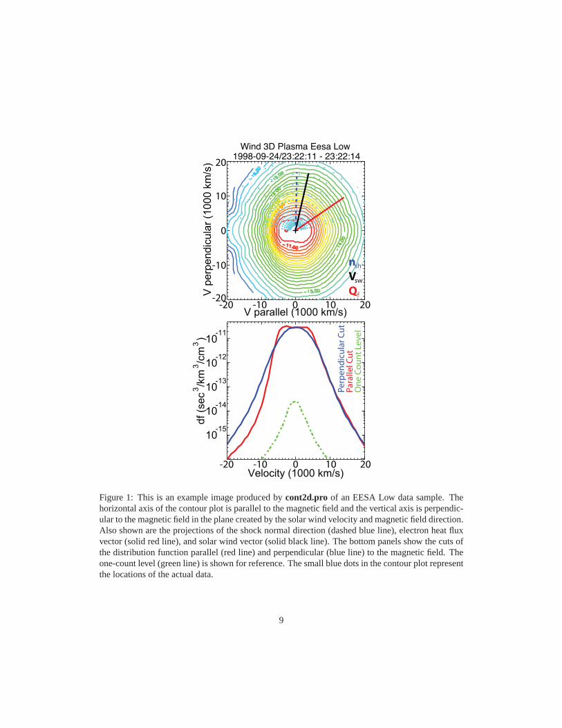
Figure 1: This is an example image produced bycont2d.pro of an EESA Low data sample. Thehorizontal axis of the contour plot is parallel to the magnetic field and the vertical axis is perpendic-ular to the magnetic field in the plane created by the solar wind velocity and magnetic field direction.Also shown are the projections of the shock normal direction(dashed blue line), electron heat fluxvector (solid red line), and solar wind vector (solid black line). The bottom panels show the cuts ofthe distribution function parallel (red line) and perpendicular (blue line) to the magnetic field. Theone-count level (green line) is shown for reference. The small blue dots in the contour plot representthe locations of the actual data.

9

3.5 IDL Implementation: Distribution Function Calculatio nsTo calculate the distribution function (DF), use the following programs (after you’ve done the

above steps):

UMN> dat = get_3dp_structs(’el’ ,TRANGE=trange)UMN> ael = dat.DATA

UMN> add_mag2,ael,’wi B3(GSE)’UMN> add_vsw2,ael,’V sw2’UMN> add_scpot,ael,’sc pot 3’

where we have added the GSE magnetic field, GSE solar wind velocity, and spacecraft potentialto ALL the data structures. Now to calculate an individual PAD and DF, perform the following:

UMN> el = ael[10]

UMN> del = convert_vframe(el,/INTERP) ; Convert into SW FrameUMN> pd = pad(del,NUM_PA=17L) ; PAD calculation; Calculate the DF nowUMN> df = distfunc(pd.ENERGY,pd.ANGLES,MASS=pd.MASS,DF=pd.DATA)

; Get the structure tags from df and put them into delUMN> extract_tags,del,df

wherepd anddf have the structure formats given by:

UMN> HELP,pd,/STRUCT,OUTPUT=houtUMN> PRINT,hout,FORMAT=’(”;”,a)’;** Structure <2122610>, 21 tags, length=14028, data length=14024, refs=1:

; PROJECT_NAME STRING ’Wind 3D Plasma’

; DATA_NAME STRING ’Eesa Low PAD’

; VALID INT 1

; UNITS_NAME STRING ’df’

; TIME DOUBLE 9.5532272e+08; END_TIME DOUBLE 9.5532272e+08; INTEG_T DOUBLE 3.1001112

; NBINS INT 17

; NENERGY LONG 15

; DATA FLOAT Array[15, 17]

; ENERGY FLOAT Array[15, 17]

; ANGLES FLOAT Array[15, 17]

; DENERGY FLOAT Array[15, 88]

; BTH FLOAT 27.2478

; BPH FLOAT -37.0210

; GF FLOAT Array[15, 17]

10

; DT FLOAT Array[15, 17]

; GEOMFACTOR DOUBLE 0.00039375000

; MASS DOUBLE 5.6856591e-06

; UNITS_PROCEDURE STRING ’convert_esa_units’

; DEADTIME FLOAT Array[15, 17]

UMN> HELP,df,/STRUCT,OUTPUT=houtUMN> PRINT,hout,FORMAT=’(”;”,a)’;** Structure <c3b4db0>, 3 tags, length=6000, data length=6000, refs=1:

; VX0 FLOAT Array[500]

; VY0 FLOAT Array[500]

; DFC FLOAT Array[500]

where the tagsVX0 and VY0 represent the parallel (with respect to the magnetic field) and per-pendicular velocities, respectively. The tagDFC is the actual estimate of the DF in units of DF(s3km−3cm−3).

One should also note that though I used 17 pitch-angles to make these structures, which isgood if there are sufficient flux levels. If the fluxes are very high, then one can get away with 24pitch-angles for EL and ELB, but I’d be wary with the other detectors.

4 Plotting the ResultsIt’s nice to have the data readily available, but what do we dowith it? Well there are couple

of ways one can look at the data. One can either plot the DF or one can plot the PAD for eachparticle structure. Note that all the plots shown in this tutorial have been cleaned up using AdobeIllustratorTM. To plot the DF as a contour plot with parallel and perpendicular cuts of the DF, do thefollowing:

UMN> dat = el

UMN> dfra = [1e-16,5e-11]

UMN> cont2d,del,VLIM=2d4,NGRID=30L,GNORM=gnorm,/HEAT_F,MYONEC=dat,DFRA=dfra

which should produce a plot like the one seen in Figure 1. The plot description is listed in thefigure caption. This figure is consistent with a flattop electron distribution [Feldman et al., 1983]and is observed downstream of a strong interplanetary shockon 1998-09-24. The small blue dotsshow where the data is actually taken in the contour plot. It is important to show these since the man-ner in which the IDL built-in function,CONTOUR.PRO, attempts to close the contours can resultin artificial distribution signatures. For instance, one can see that the data is not sampled perfectlyalong the magnetic field (horizontal axis of contour plot) but at a small angle (&10◦). This anglecan often be much higher, yet IDL will still make the contoursappear as though there is a beam-likesignature parallel or anti-parallel to the magnetic field. Also, often times low energy beam-like sig-natures appear in the data, but they can occasionally occur at a velocity which is inside the lowest

11

Wind 3D PlasmaEesa Low PAD

2000-04-06/16:22:20 - 16:22:23

689.2 eV

426.8 eV

264.8 eV

169.0 eV

103.3 eV

65.2 eV

41.8 eV

27.2 eV

1113.0 eV

689.2 eV

426.8 eV

264.8 eV

169.0 eV

103.3 eV

65.2 eV

41.8 eV

27.2 eV

1113.0 eV

90 1800Pitch Angle (degrees)

EF

lux (

eV

/ s

ec / c

m / ste

r / e

V)

2 107

108

106

105

Flu

x (

# / s

ec / c

m / ste

r / e

V)

2

103

104

105

106

102

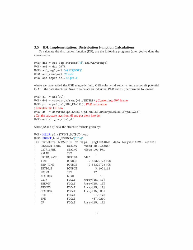
Figure 2: This is an example image produced bymy padplot both.pro using UNITS=’flux’ for anEESA Low data sample. The top panel is a stacked line plot of the pitch-angle distributions at the9 highest energies in units of number flux. The bottom panel isthe same thing except in units ofenergy flux. The vertical axes are logarithmically scaled while the horizontal axes range from 0◦ to180◦.

12

Wind 3DP Pesa High Burst2000-02-11/23:34:02 - 23:34:05

Velocity [km/s]-2 -1 0 1 2

-2

-1

0

1

2

Vp

erp

[1

00

0 k

m/s

]

-2 -1 0 1 2Vpara [1000 km/s]

33

3d

f (s

ec /k

m /c

m )

10-13

10-11

10-12

10-10

10-9

Pe

rpe

nd

icu

lar

Cu

tP

ara

lle

l Cu

tO

ne

Co

un

t Le

ve

l

Sun Dir.

Vsw

nsh

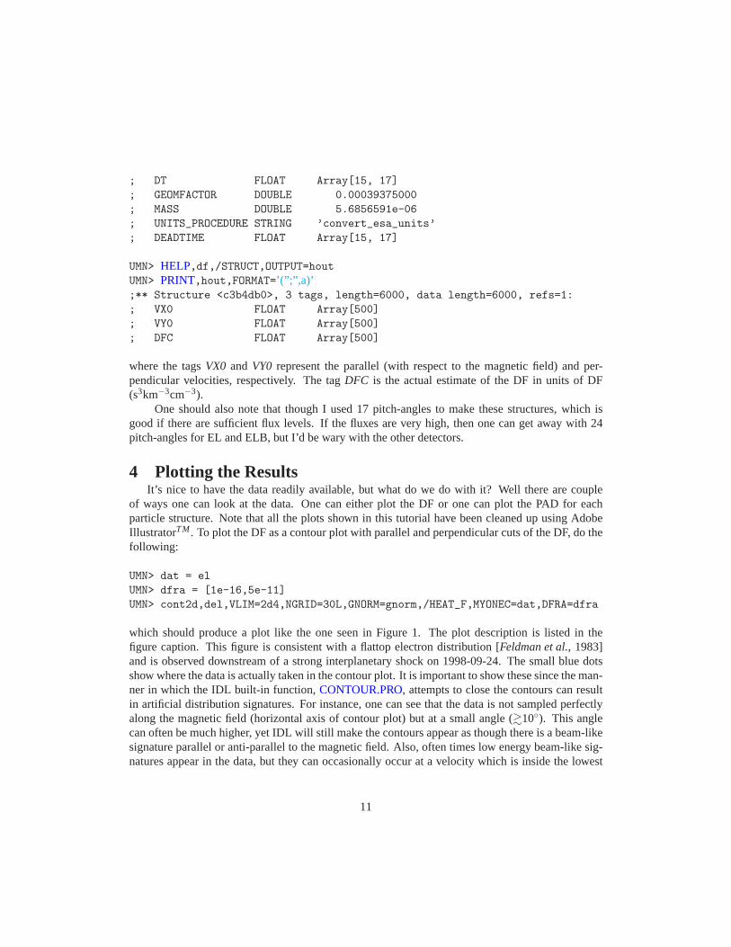
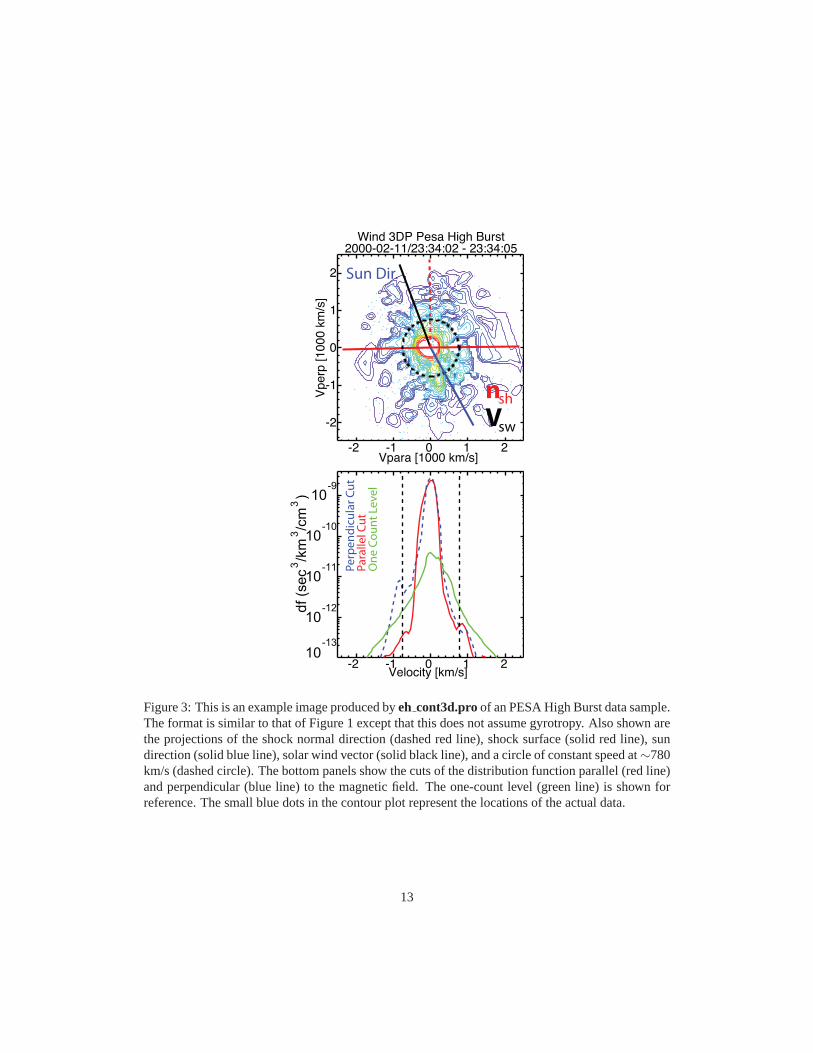
Figure 3: This is an example image produced byeh cont3d.proof an PESA High Burst data sample.The format is similar to that of Figure 1 except that this doesnot assume gyrotropy. Also shown arethe projections of the shock normal direction (dashed red line), shock surface (solid red line), sundirection (solid blue line), solar wind vector (solid blackline), and a circle of constant speed at∼780km/s (dashed circle). The bottom panels show the cuts of the distribution function parallel (red line)and perpendicular (blue line) to the magnetic field. The one-count level (green line) is shown forreference. The small blue dots in the contour plot representthe locations of the actual data.

13

velocity available (due to SC potential and reference frametransformation effects). These signalsshould NOT be trusted as they are artifacts of IDL, NOT the data!

To plot the PADs in a useful manner, one can use eitherpadplot.pro or my padplot both.pro.The former will produce a single plot of the PAD with in one setof units while the latter will producetwo plots as seen in Figure 2. To produce the PAD plot, do the following:

UMN> my_padplot_both,pd,UNITS=’flux’ EBINS=[0L,8L]

The other detector in which one might wish to view the distribution functions of is PH. Themanner in which the DF is calculated for PH is slightly different and somewhat more complicateddue to a number of sources of noise etc. Regardless, assume you have already retrieved particlestructures for PH in a similar manner to the one used to get theEL structures above4, then do thefollowing:

UMN> aphb = dat.DATA

UMN> dat = aphb[10]

UMN> ngrid = 20L

UMN> vlim = 25e2

UMN> sunv = [1.,0.,0.]

UMN> sunn = ’Sun Dir.’

UMN> vcirc = 780.

UMN> eh_cont3d,dat,VLIM=vlim,NGRID=ngrid,/SM_CUTS,EX_VEC=sunv,EX_VN=sunn,VCIRC=vcirc[0],/ONE_C

which should produce a plot like the one seen in Figure 3. The format of Figure 3 is similar tothat of Figure 1.

4.1 IDL Implementation: Tensor Rotations and ManipulationsTo begin with, I will illustrate the tensor and array notation used in IDL to help the user be-

come familiar with the calculations being done in the programs used. If you aren’t concerned withthese particulars, you can skip to the next section for the IDL commands. The two programs whichwill calculate the heat flux vector and tensor from a given 3DPparticle distribution structure aremom sum.proandmom translate.pro. The programs were initially uncommented and impossiblyopaque. I have since gone through and commented and/or explained certain aspects of these pro-grams which should help a well prepared expert use them. However, a beginning graduate studentmight find them far beyond what they deem themself capable of understanding. So I will try andhelp illustrate, in this section, the more complicated and semi-opaque steps one finds in these tworoutines. Much ofmom sum.pro is commented which makes it pretty straight forward. The op-erations inmom translate.probecome remarkably complicated in the sense that comments mightrequire more space than isethically allowed under decent programing standards. So I’ll try andilluminate as many of these opaque andmessysteps as possible.

4Use PHB and short time ranges here to avoid multiple mapcodes

14

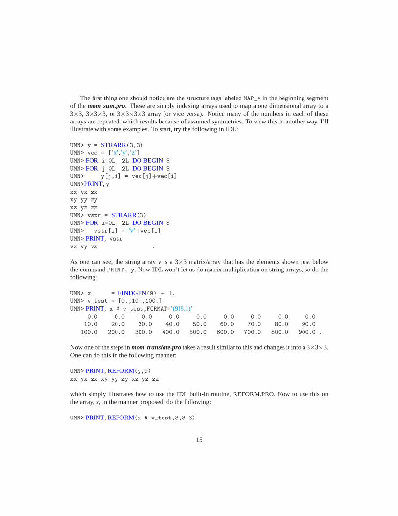
The first thing one should notice are the structure tags labeledMAP_* in the beginning segmentof themom sum.pro. These are simply indexing arrays used to map a one dimensional array to a3×3, 3×3×3, or 3×3×3×3 array (or vice versa). Notice many of the numbers in each of thesearrays are repeated, which results because of assumed symmetries. To view this in another way, I’llillustrate with some examples. To start, try the following in IDL:

UMN> y = STRARR(3,3)UMN> vec = [’x’ ,’y’ ,’z’ ]UMN> FOR i=0L, 2L DO BEGIN $

UMN> FOR j=0L, 2L DO BEGIN $

UMN> y[j,i] = vec[j]+vec[i]UMN>PRINT, yxx yx zx

xy yy zy

xz yz zz

UMN> vstr = STRARR(3)UMN> FOR i=0L, 2L DO BEGIN $

UMN> vstr[i] = ’v’ +vec[i]UMN> PRINT, vstr

vx vy vz .

As one can see, the string arrayy is a 3×3 matrix/array that has the elements shown just belowthe commandPRINT, y. Now IDL won’t let us do matrix multiplication on string arrays, so do thefollowing:

UMN> x = FINDGEN(9) + 1.

UMN> v_test = [0.,10.,100.]

UMN> PRINT, x # v_test,FORMAT=’(9f8.1)’0.0 0.0 0.0 0.0 0.0 0.0 0.0 0.0 0.0

10.0 20.0 30.0 40.0 50.0 60.0 70.0 80.0 90.0

100.0 200.0 300.0 400.0 500.0 600.0 700.0 800.0 900.0 .

Now one of the steps inmom translate.protakes a result similar to this and changes it into a 3×3×3.One can do this in the following manner:

UMN> PRINT, REFORM(y,9)xx yx zx xy yy zy xz yz zz

which simply illustrates how to use the IDL built-in routine, REFORM.PRO. Now to use this onthe array,x, in the manner proposed, do the following:

UMN> PRINT, REFORM(x # v_test,3,3,3)

15

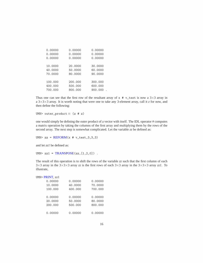
0.00000 0.00000 0.00000

0.00000 0.00000 0.00000

0.00000 0.00000 0.00000

10.0000 20.0000 30.0000

40.0000 50.0000 60.0000

70.0000 80.0000 90.0000

100.000 200.000 300.000

400.000 500.000 600.000

700.000 800.000 900.000 .

Thus one can see that the first row of the resultant array ofx # v_test is now a 3×3 array ina 3×3×3 array. It is worth noting that were one to take any 3-elementarray, call itz for now, andthen define the following:

UMN> outer_product ≡ (z # z)

one would simply be defining the outer product of a vector withitself. The IDL operator # computesa matrix operation by taking the columns of the first array andmultiplying them by the rows of thesecond array. The next step is somewhat complicated. Let thevariablezzbe defined as:

UMN> zz = REFORM(x # v_test,3,3,3)

and letzz1be defined as:

UMN> zz1 = TRANSPOSE(zz,[1,2,0]) .

The result of this operation is to shift the rows of the variable zzsuch that the first column of each3×3 array in the 3×3×3 arrayzz is the first rows of each 3×3 array in the 3×3×3 arrayzz1. Toillustrate,

UMN> PRINT, zz10.00000 0.00000 0.00000

10.0000 40.0000 70.0000

100.000 400.000 700.000

0.00000 0.00000 0.00000

20.0000 50.0000 80.0000

200.000 500.000 800.000

0.00000 0.00000 0.00000

16

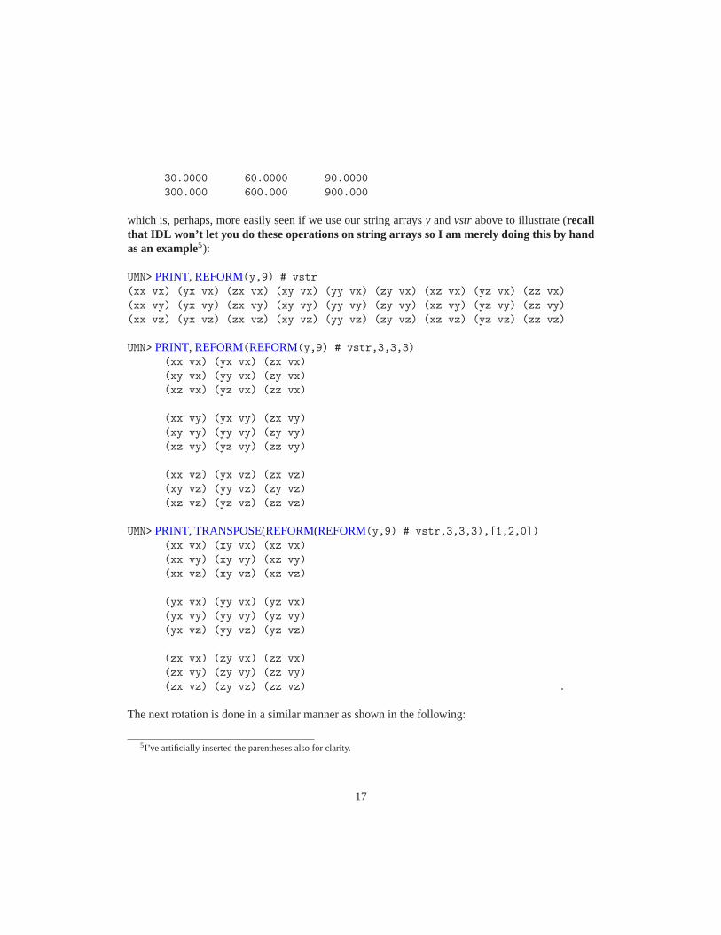
30.0000 60.0000 90.0000

300.000 600.000 900.000

which is, perhaps, more easily seen if we use our string arrays y andvstr above to illustrate (recallthat IDL won’t let you do these operations on string arrays soI am merely doing this by handas an example5):

UMN> PRINT, REFORM(y,9) # vstr

(xx vx) (yx vx) (zx vx) (xy vx) (yy vx) (zy vx) (xz vx) (yz vx) (zz vx)

(xx vy) (yx vy) (zx vy) (xy vy) (yy vy) (zy vy) (xz vy) (yz vy) (zz vy)

(xx vz) (yx vz) (zx vz) (xy vz) (yy vz) (zy vz) (xz vz) (yz vz) (zz vz)

UMN> PRINT, REFORM(REFORM(y,9) # vstr,3,3,3)

(xx vx) (yx vx) (zx vx)

(xy vx) (yy vx) (zy vx)

(xz vx) (yz vx) (zz vx)

(xx vy) (yx vy) (zx vy)

(xy vy) (yy vy) (zy vy)

(xz vy) (yz vy) (zz vy)

(xx vz) (yx vz) (zx vz)

(xy vz) (yy vz) (zy vz)

(xz vz) (yz vz) (zz vz)

UMN> PRINT, TRANSPOSE(REFORM(REFORM(y,9) # vstr,3,3,3),[1,2,0])

(xx vx) (xy vx) (xz vx)

(xx vy) (xy vy) (xz vy)

(xx vz) (xy vz) (xz vz)

(yx vx) (yy vx) (yz vx)

(yx vy) (yy vy) (yz vy)

(yx vz) (yy vz) (yz vz)

(zx vx) (zy vx) (zz vx)

(zx vy) (zy vy) (zz vy)

(zx vz) (zy vz) (zz vz) .

The next rotation is done in a similar manner as shown in the following:

5I’ve artificially inserted the parentheses also for clarity.

17

UMN>PRINT, TRANSPOSE( REFORM( REFORM(y,9) # vstr,3,3,3),[2,0,1])

(xx vx) (xx vy) (xx vz)

(yx vx) (yx vy) (yx vz)

(zx vx) (zx vy) (zx vz)

(xy vx) (xy vy) (xy vz)

(yy vx) (yy vy) (yy vz)

(zy vx) (zy vy) (zy vz)

(xz vx) (xz vy) (xz vz)

(yz vx) (yz vy) (yz vz)

(zz vx) (zz vy) (zz vz) .

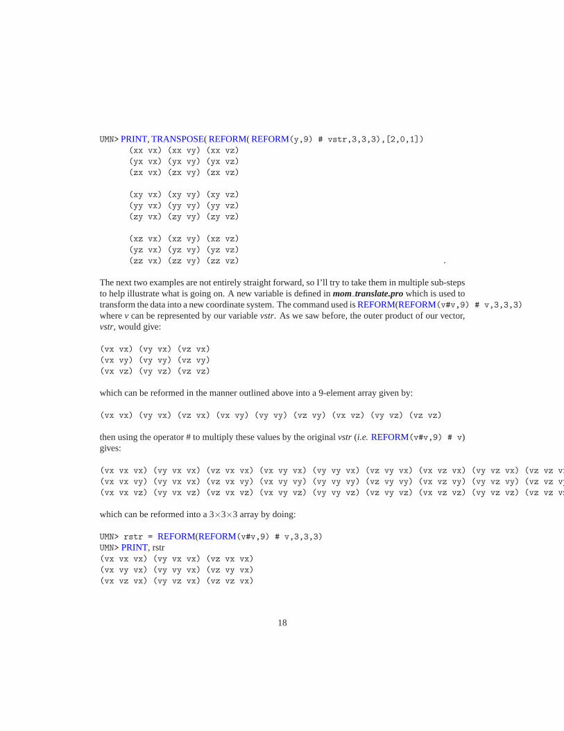
The next two examples are not entirely straight forward, so I’ll try to take them in multiple sub-stepsto help illustrate what is going on. A new variable is defined in mom translate.prowhich is used totransform the data into a new coordinate system. The commandused isREFORM(REFORM(v#v,9) # v,3,3,3)

wherev can be represented by our variablevstr. As we saw before, the outer product of our vector,vstr, would give:

(vx vx) (vy vx) (vz vx)

(vx vy) (vy vy) (vz vy)

(vx vz) (vy vz) (vz vz)

which can be reformed in the manner outlined above into a 9-element array given by:

(vx vx) (vy vx) (vz vx) (vx vy) (vy vy) (vz vy) (vx vz) (vy vz) (vz vz)

then using the operator # to multiply these values by the original vstr (i.e. REFORM(v#v,9) # v)gives:

(vx vx vx) (vy vx vx) (vz vx vx) (vx vy vx) (vy vy vx) (vz vy vx) (vx vz vx) (vy vz vx) (vz vz vx)

(vx vx vy) (vy vx vx) (vz vx vy) (vx vy vy) (vy vy vy) (vz vy vy) (vx vz vy) (vy vz vy) (vz vz vy)

(vx vx vz) (vy vx vz) (vz vx vz) (vx vy vz) (vy vy vz) (vz vy vz) (vx vz vz) (vy vz vz) (vz vz vz)

which can be reformed into a 3×3×3 array by doing:

UMN> rstr = REFORM(REFORM(v#v,9) # v,3,3,3)

UMN> PRINT, rstr(vx vx vx) (vy vx vx) (vz vx vx)

(vx vy vx) (vy vy vx) (vz vy vx)

(vx vz vx) (vy vz vx) (vz vz vx)

18

(vx vx vy) (vy vx vx) (vz vx vy)

(vx vy vy) (vy vy vy) (vz vy vy)

(vx vz vy) (vy vz vy) (vz vz vy)

(vx vx vz) (vy vx vz) (vz vx vz)

(vx vy vz) (vy vy vz) (vz vy vz)

(vx vz vz) (vy vz vz) (vz vz vz).

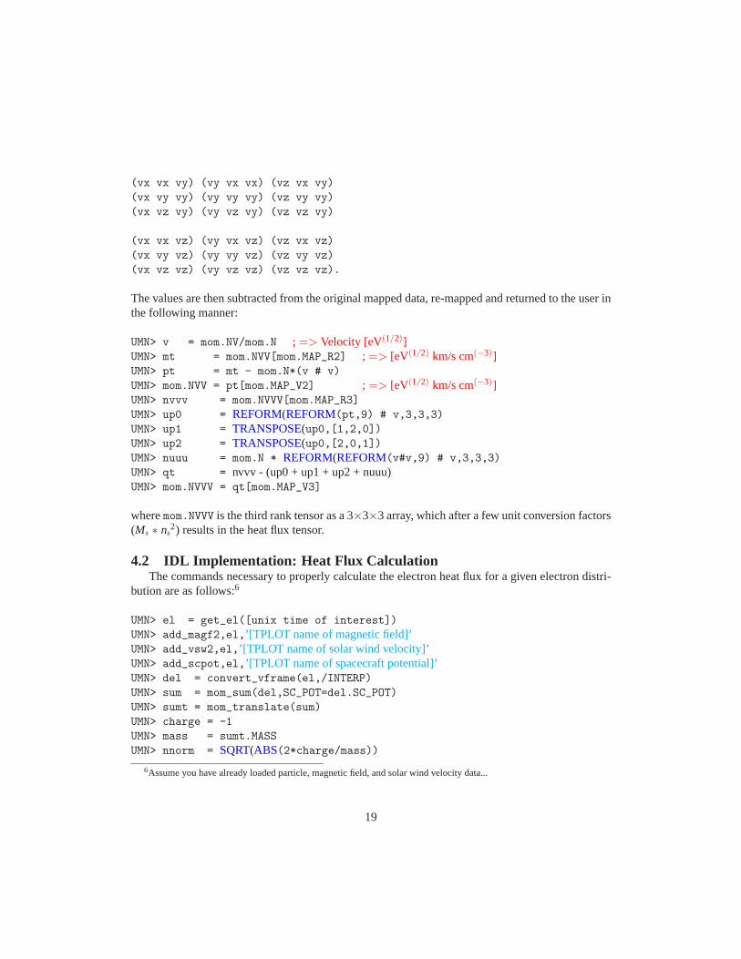
The values are then subtracted from the original mapped data, re-mapped and returned to the user inthe following manner:

UMN> v = mom.NV/mom.N ; => Velocity [eV(1/2)]UMN> mt = mom.NVV[mom.MAP_R2] ; => [eV(1/2) km/s cm(−3)]UMN> pt = mt - mom.N*(v # v)

UMN> mom.NVV = pt[mom.MAP_V2] ; => [eV(1/2) km/s cm(−3)]UMN> nvvv = mom.NVVV[mom.MAP_R3]

UMN> up0 = REFORM(REFORM(pt,9) # v,3,3,3)

UMN> up1 = TRANSPOSE(up0,[1,2,0])UMN> up2 = TRANSPOSE(up0,[2,0,1])UMN> nuuu = mom.N * REFORM(REFORM(v#v,9) # v,3,3,3)

UMN> qt = nvvv - (up0 + up1 + up2 + nuuu)UMN> mom.NVVV = qt[mom.MAP_V3]

wheremom.NVVV is the third rank tensor as a 3×3×3 array, which after a few unit conversion factors(Ms ∗ ns

2) results in the heat flux tensor.

4.2 IDL Implementation: Heat Flux CalculationThe commands necessary to properly calculate the electron heat flux for a given electron distri-

bution are as follows:6

UMN> el = get_el([unix time of interest])

UMN> add_magf2,el,’[TPLOT name of magnetic field]’UMN> add_vsw2,el,’[TPLOT name of solar wind velocity]’UMN> add_scpot,el,’[TPLOT name of spacecraft potential]’UMN> del = convert_vframe(el,/INTERP)

UMN> sum = mom_sum(del,SC_POT=del.SC_POT)

UMN> sumt = mom_translate(sum)

UMN> charge = -1

UMN> mass = sumt.MASS

UMN> nnorm = SQRT(ABS(2*charge/mass))

6Assume you have already loaded particle, magnetic field, and solar wind velocity data...

19

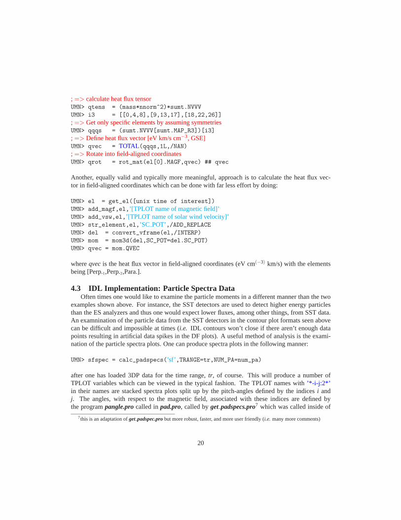
; => calculate heat flux tensorUMN> qtens = (mass*nnorm^2)*sumt.NVVV

UMN> i3 = [[0,4,8],[9,13,17],[18,22,26]]

; => Get only specific elements by assuming symmetriesUMN> qqqs = (sumt.NVVV[sumt.MAP_R3])[i3]

; => Define heat flux vector [eV km/s cm−3, GSE]UMN> qvec = TOTAL(qqqs,1L,/NAN); => Rotate into field-aligned coordinatesUMN> qrot = rot_mat(el[0].MAGF,qvec) ## qvec

Another, equally valid and typically more meaningful, approach is to calculate the heat flux vec-tor in field-aligned coordinates which can be done with far less effort by doing:

UMN> el = get_el([unix time of interest])

UMN> add_magf,el,’[TPLOT name of magnetic field]’UMN> add_vsw,el,’[TPLOT name of solar wind velocity]’UMN> str_element,el,’SC POT’,/ADD_REPLACEUMN> del = convert_vframe(el,/INTERP)

UMN> mom = mom3d(del,SC_POT=del.SC_POT)

UMN> qvec = mom.QVEC

whereqvecis the heat flux vector in field-aligned coordinates (eV cm(−3) km/s) with the elementsbeing [Perp.1,Perp.2,Para.].

4.3 IDL Implementation: Particle Spectra DataOften times one would like to examine the particle moments ina different manner than the two

examples shown above. For instance, the SST detectors are used to detect higher energy particlesthan the ES analyzers and thus one would expect lower fluxes, among other things, from SST data.An examnination of the particle data from the SST detectors in the contour plot formats seen abovecan be difficult and impossible at times (i.e. IDL contours won’t close if there aren’t enough datapoints resulting in artificial data spikes in the DF plots). Auseful method of analysis is the exami-nation of the particle spectra plots. One can produce spectra plots in the following manner:

UMN> sfspec = calc_padspecs(’sf’ ,TRANGE=tr,NUM_PA=num_pa)

after one has loaded 3DP data for the time range,tr, of course. This will produce a number ofTPLOT variables which can be viewed in the typical fashion. The TPLOT names with’*-i-j:2*’in their names are stacked spectra plots split up by the pitch-angles defined by the indicesi andj. The angles, with respect to the magnetic field, associated with these indices are defined bythe programpangle.procalled inpad.pro, called byget padspecs.pro7 which was called inside of

7this is an adaptation ofget padspec.probut more robust, faster, and more user friendly (i.e. many more comments)

20

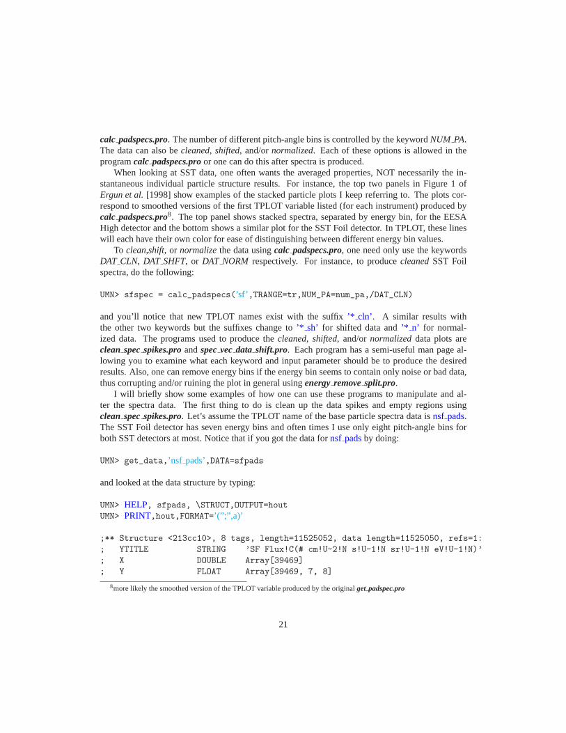
calc padspecs.pro. The number of different pitch-angle bins is controlled by the keywordNUM PA.The data can also becleaned, shifted, and/ornormalized. Each of these options is allowed in theprogramcalc padspecs.proor one can do this after spectra is produced.

When looking at SST data, one often wants the averaged properties, NOT necessarily the in-stantaneous individual particle structure results. For instance, the top two panels in Figure 1 ofErgun et al.[1998] show examples of the stacked particle plots I keep referring to. The plots cor-respond to smoothed versions of the first TPLOT variable listed (for each instrument) produced bycalc padspecs.pro8. The top panel shows stacked spectra, separated by energy bin, for the EESAHigh detector and the bottom shows a similar plot for the SST Foil detector. In TPLOT, these lineswill each have their own color for ease of distinguishing between different energy bin values.

To clean,shift, or normalizethe data usingcalc padspecs.pro, one need only use the keywordsDAT CLN, DAT SHFT, or DAT NORM respectively. For instance, to producecleanedSST Foilspectra, do the following:

UMN> sfspec = calc_padspecs(’sf’ ,TRANGE=tr,NUM_PA=num_pa,/DAT_CLN)

and you’ll notice that new TPLOT names exist with the suffix’* cln’. A similar results withthe other two keywords but the suffixes change to’* sh’ for shifted data and’* n’ for normal-ized data. The programs used to produce thecleaned, shifted, and/ornormalizeddata plots areclean specspikes.proandspecvecdata shift.pro. Each program has a semi-useful man page al-lowing you to examine what each keyword and input parameter should be to produce the desiredresults. Also, one can remove energy bins if the energy bin seems to contain only noise or bad data,thus corrupting and/or ruining the plot in general usingenergyremovesplit.pro.

I will briefly show some examples of how one can use these programs to manipulate and al-ter the spectra data. The first thing to do is clean up the data spikes and empty regions usingclean specspikes.pro. Let’s assume the TPLOT name of the base particle spectra data isnsf pads.The SST Foil detector has seven energy bins and often times I use only eight pitch-angle bins forboth SST detectors at most. Notice that if you got the data fornsf padsby doing:

UMN> get_data,’nsf pads’,DATA=sfpads

and looked at the data structure by typing:

UMN> HELP, sfpads, \STRUCT,OUTPUT=hout

UMN> PRINT,hout,FORMAT=’(”;”,a)’

;** Structure <213cc10>, 8 tags, length=11525052, data length=11525050, refs=1:

; YTITLE STRING ’SF Flux!C(# cm!U-2!N s!U-1!N sr!U-1!N eV!U-1!N)’

; X DOUBLE Array[39469]

; Y FLOAT Array[39469, 7, 8]

8more likely the smoothed version of the TPLOT variable produced by the originalget padspec.pro

21

; V1 FLOAT Array[39469, 7]

; V2 FLOAT Array[39469, 8]

; YLOG INT 1

; LABELS STRING Array[7]

; PANEL_SIZE FLOAT 2.00000

where the number39469refers to the number of different particle structures (i.e. time steps) inthe data,7 is the number of energy bins, and8 is the number of pitch-angles. Note that the TPLOTstructure above is a standard format for 3-dimensional dataarrays depending on time and two otherquantities. The tagsX andY are the Unix time and data, respectively, as usual and the tags V1 andV2 refer to the particle energies and pitch-angles, respectively. The plot resulting from these wouldbe an average overV2, thus an effective omni-directional spectra. If we look at aTPLOT variablewhich as already been split up by the programsreducepads.proandreducedimen.pro, we’ll finda slightly different structure format. To do so, do the following:

UMN> get_data,’nsf pads-2-0:1’,DATA=sfpd01UMN> HELP, sfpd01, \STRUCT,OUTPUT=hout

UMN> PRINT,hout,FORMAT=’(”;”,a)’

;** Structure <1dc3500>, 3 tags, length=2526016, data length=2526016, refs=1:

; X DOUBLE Array[39469]

; Y FLOAT Array[39469, 7]

; V FLOAT Array[39469, 7]

where only the tagV now exists in place ofV1 and V2 corresponding to the energies for eachelement ofY. So now let’s smooth out the data spikes innsf padsby smoothing over 7 points in thelower energies and 10 points in the two highest energies by doing:

UMN> oldnn = ’nsf pads’UMN> newnn = ’nsf padscln’UMN> nsmth = 7

UMN> esmth = [0L,1L,10L]

UMN> clean_spec_spikes,oldnn,NEW_NAME=newnn,NSMOOTH=nsmth,ESMOOTH=esmth

which will produce a new TPLOT variable namednsf padscln. To shift the four highest ener-gies of the data, do the following:

UMN> newnn = ’nsf padssh’UMN> spec_vec_data_shift,oldnn,NEW_NAME=newnn,WSHIFT=[0L,3L]

and to shift AND normalize the data, do the following:

22

UMN> newnn = ’nsf padssh n’UMN> spec_vec_data_shift,oldnn,NEW_NAME=newnn,/DATS,/DATN

Let’s say that the two highest energy bins appear to be only noise and they are skewing your Y-Axis limits making the plot impossible to read. To remove these two energy bins, do the following:

UMN> newnn = ’nsf pads5-Lowest-E’UMN> energy_remove_split,oldnn,NEW_NAME1=newnn,ENERGIES=[0,1]

Notice that the program redetermines the colors, TPLOT labels, and the vertical axis range foryou. If the two highest energies weren’t noise, but they appeared to be interesting also, we couldsplit the energy ranges into low and high by doing the following:

UMN> newnl = ’nsf pads5-Lowest-E’UMN> newnh = ’nsf pads2-Highest-E’UMN> energy_remove_split,oldnn,NEW_NAME1=newnl,NEW_NAME2=newnh,ENERGIES=[0,1],/SPLIT

5 The Pesa High GlitchOn occasion, the PH detector has aglitch in the data which always occurs in the same data bins,

regardless of data/time. I use the termglitch, though the bad bins result from things which are notlikely due to an electronic glitch or anything like that. In fact, the consistency of the bin numbersbeing affected and their relation to the sun direction suggests that the issue is more likely due to UVcontamination than an electronic glitch. There are also issues with saturation in the ecliptic planedue to the detectors large geometry factor and the high flux rate of the solar wind. The energy binsshow a pattern suggesting these bins may relate to the bins inthe double-sweep mode, since theenergies go from∼28 keV down to∼5 keV then start over again. Regardless, the counts associatedwith these data bins are clearly not physical as they often exceed 2-3 orders of magnitude above thecounts in the rest of the detector bins9. If the data structures are retrieved on a Sun Machine, theerror in the energy bin values will occur as a NaN and the corresponding data values will be toolarge to be physically reliable. If the data structures are retrieved on a Mac, the bad values turn intovery large numbers. The issue is results from the definition of big and little endian for the Mac Inteland Sun Machine shared object libraries.

The glitches occur consistently in the same data bins, regardless of day or year. The bins, how-ever, depend upon the mode that the Pesa High detector is in. Ihave found the following bins to bean issue for the sample modes seen in Table 1. The only two modes I have yet to find aglitch in arethe two where the number of bins equals 65 or 88. This is largely due to the fact that I almost neverfind Pesa High in a sample mode with these number of data bins.

I have written two programs to help deal with this issue,pesahigh bad bins.pro andpesahigh str fill.pro .Both programs attempt to handle this issue and they are called by multiple other programs in my list

9Perhaps this is a combination of UV contamination and the high solar wind flux.

23

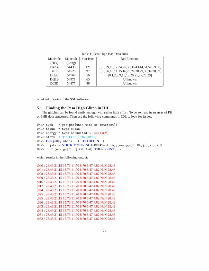
Table 1: Pesa High Bad Data Bins

Mapcode Mapcode # of Bins Bin Elements(Hex) (Long)D4A4 54436 121 [0,1,8,9,16,17,24,25,35,36,43,44,51,52,59,60]D4FE 54526 97 [0,1,5,6,10,11,15,16,23,24,28,29,33,34,38,39]D5EC 54764 56 [0,1,2,8,9,10,19,20,21,27,28,29]D6BB 54971 65 UnknownD65D 54877 88 Unknown

of added libraries to the SSL software.

5.1 Finding the Pesa High Glitch in IDLThe glitches can be found easily enough with rather little effort. To do so, read in an array of PH

or PHB data structures. Then use the following commands in IDL to look for issues:

UMN> twph = get_ph([unix time of interest])

UMN> nbins = twph.NBINS

UMN> energy = twph.ENERGY*1d-3 ; => (keV)UMN> mform = ’(”;”,I3.3,” : ”,f6.2,8f9.2)’UMN> FORj=0L, nbins - 1L DO BEGIN $

UMN> jstr = STRTRIM(STRING(FORMAT=mform,j,energy[0L:8L,j]),2L) & $

UMN> IF (energy[8L,j] GT 4e0) THEN PRINT, jstr

which results in the following output:

;000 : 28.43 21.15 15.73 11.70 8.70 6.47 4.82 NaN 28.43;001 : 28.43 21.15 15.73 11.70 8.70 6.47 4.82 NaN 28.43;008 : 28.43 21.15 15.73 11.70 8.70 6.47 4.82 NaN 28.43;009 : 28.43 21.15 15.73 11.70 8.70 6.47 4.82 NaN 28.43;016 : 28.43 21.15 15.73 11.70 8.70 6.47 4.82 NaN 28.43;017 : 28.43 21.15 15.73 11.70 8.70 6.47 4.82 NaN 28.43;024 : 28.43 21.15 15.73 11.70 8.70 6.47 4.82 NaN 28.43;025 : 28.43 21.15 15.73 11.70 8.70 6.47 4.82 NaN 28.43;035 : 28.43 21.15 15.73 11.70 8.70 6.47 4.82 NaN 28.43;036 : 28.43 21.15 15.73 11.70 8.70 6.47 4.82 NaN 28.43;043 : 28.43 21.15 15.73 11.70 8.70 6.47 4.82 NaN 28.43;044 : 28.43 21.15 15.73 11.70 8.70 6.47 4.82 NaN 28.43;051 : 28.43 21.15 15.73 11.70 8.70 6.47 4.82 NaN 28.43;052 : 28.43 21.15 15.73 11.70 8.70 6.47 4.82 NaN 28.43

24

;059 : 28.43 21.15 15.73 11.70 8.70 6.47 4.82 NaN 28.43;060 : 28.43 21.15 15.73 11.70 8.70 6.47 4.82 NaN 28.43.

Notice that the seventh (indexing from zero since in IDL) element isNot A Numberor NaN. Theeighth element seems to start back at the highest energy and repeat the pattern, as seen below withthe following commands:

UMN> twph = get_ph([unix time of interest])

UMN> nbins = twph.NBINS

UMN> energy = twph.ENERGY*1d-3 ; => (keV)UMN> mform = ’(”;”,I3.3,” : ”,f6.2,5f9.2)’UMN> FORj=0L, nbins - 1L DO BEGIN $

UMN> jstr = STRTRIM(STRING(FORMAT=mform,j,energy[9L:14L,j]),2L) & $

UMN> IF (energy[8L,j] GT 4e0) THEN PRINT, jstr

which results in the following output:

;000 : 21.15 15.73 11.70 8.70 6.47 4.82;001 : 21.15 15.73 11.70 8.70 6.47 4.82;008 : 21.15 15.73 11.70 8.70 6.47 4.82;009 : 21.15 15.73 11.70 8.70 6.47 4.82;016 : 21.15 15.73 11.70 8.70 6.47 4.82;017 : 21.15 15.73 11.70 8.70 6.47 4.82;024 : 21.15 15.73 11.70 8.70 6.47 4.82;025 : 21.15 15.73 11.70 8.70 6.47 4.82;035 : 21.15 15.73 11.70 8.70 6.47 4.82;036 : 21.15 15.73 11.70 8.70 6.47 4.82;043 : 21.15 15.73 11.70 8.70 6.47 4.82;044 : 21.15 15.73 11.70 8.70 6.47 4.82;051 : 21.15 15.73 11.70 8.70 6.47 4.82;052 : 21.15 15.73 11.70 8.70 6.47 4.82;059 : 21.15 15.73 11.70 8.70 6.47 4.82;060 : 21.15 15.73 11.70 8.70 6.47 4.82.

The glitch appears always at the same azimuthal angles,φ (degrees), in the Pesa High datastructures. To find them, follow a similar procedure as outlined above, but changeenergyto phi inthe variable definition ofjstr. The angles are as follows:

;000 : 179.62 178.88 178.12 177.38 176.62 175.88 175.12 174.38 173.62;001 : 179.62 178.88 178.12 177.38 176.62 175.88 175.12 174.38 173.62;002 : 179.62 178.88 178.12 177.38 176.62 175.88 175.12 174.38 173.62;008 : 190.88 190.12 189.38 188.62 187.88 187.12 186.38 185.62 184.88

25

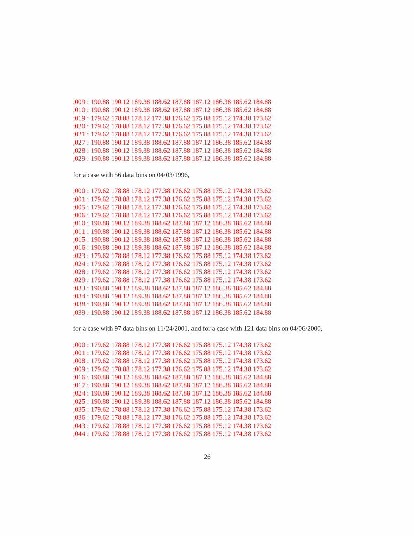
;009 : 190.88 190.12 189.38 188.62 187.88 187.12 186.38 185.62 184.88;010 : 190.88 190.12 189.38 188.62 187.88 187.12 186.38 185.62 184.88;019 : 179.62 178.88 178.12 177.38 176.62 175.88 175.12 174.38 173.62;020 : 179.62 178.88 178.12 177.38 176.62 175.88 175.12 174.38 173.62;021 : 179.62 178.88 178.12 177.38 176.62 175.88 175.12 174.38 173.62;027 : 190.88 190.12 189.38 188.62 187.88 187.12 186.38 185.62 184.88;028 : 190.88 190.12 189.38 188.62 187.88 187.12 186.38 185.62 184.88;029 : 190.88 190.12 189.38 188.62 187.88 187.12 186.38 185.62 184.88

for a case with 56 data bins on 04/03/1996,

;000 : 179.62 178.88 178.12 177.38 176.62 175.88 175.12 174.38 173.62;001 : 179.62 178.88 178.12 177.38 176.62 175.88 175.12 174.38 173.62;005 : 179.62 178.88 178.12 177.38 176.62 175.88 175.12 174.38 173.62;006 : 179.62 178.88 178.12 177.38 176.62 175.88 175.12 174.38 173.62;010 : 190.88 190.12 189.38 188.62 187.88 187.12 186.38 185.62 184.88;011 : 190.88 190.12 189.38 188.62 187.88 187.12 186.38 185.62 184.88;015 : 190.88 190.12 189.38 188.62 187.88 187.12 186.38 185.62 184.88;016 : 190.88 190.12 189.38 188.62 187.88 187.12 186.38 185.62 184.88;023 : 179.62 178.88 178.12 177.38 176.62 175.88 175.12 174.38 173.62;024 : 179.62 178.88 178.12 177.38 176.62 175.88 175.12 174.38 173.62;028 : 179.62 178.88 178.12 177.38 176.62 175.88 175.12 174.38 173.62;029 : 179.62 178.88 178.12 177.38 176.62 175.88 175.12 174.38 173.62;033 : 190.88 190.12 189.38 188.62 187.88 187.12 186.38 185.62 184.88;034 : 190.88 190.12 189.38 188.62 187.88 187.12 186.38 185.62 184.88;038 : 190.88 190.12 189.38 188.62 187.88 187.12 186.38 185.62 184.88;039 : 190.88 190.12 189.38 188.62 187.88 187.12 186.38 185.62 184.88

for a case with 97 data bins on 11/24/2001, and for a case with 121 data bins on 04/06/2000,

;000 : 179.62 178.88 178.12 177.38 176.62 175.88 175.12 174.38 173.62;001 : 179.62 178.88 178.12 177.38 176.62 175.88 175.12 174.38 173.62;008 : 179.62 178.88 178.12 177.38 176.62 175.88 175.12 174.38 173.62;009 : 179.62 178.88 178.12 177.38 176.62 175.88 175.12 174.38 173.62;016 : 190.88 190.12 189.38 188.62 187.88 187.12 186.38 185.62 184.88;017 : 190.88 190.12 189.38 188.62 187.88 187.12 186.38 185.62 184.88;024 : 190.88 190.12 189.38 188.62 187.88 187.12 186.38 185.62 184.88;025 : 190.88 190.12 189.38 188.62 187.88 187.12 186.38 185.62 184.88;035 : 179.62 178.88 178.12 177.38 176.62 175.88 175.12 174.38 173.62;036 : 179.62 178.88 178.12 177.38 176.62 175.88 175.12 174.38 173.62;043 : 179.62 178.88 178.12 177.38 176.62 175.88 175.12 174.38 173.62;044 : 179.62 178.88 178.12 177.38 176.62 175.88 175.12 174.38 173.62

26

;051 : 190.88 190.12 189.38 188.62 187.88 187.12 186.38 185.62 184.88;052 : 190.88 190.12 189.38 188.62 187.88 187.12 186.38 185.62 184.88;059 : 190.88 190.12 189.38 188.62 187.88 187.12 186.38 185.62 184.88;060 : 190.88 190.12 189.38 188.62 187.88 187.12 186.38 185.62 184.88.

In each case we see a repeating pattern, as with the data bins,consistent with the spacecraft rotationrate remaining approximately the same, within the angular resolution of the Pesa High detector.

27

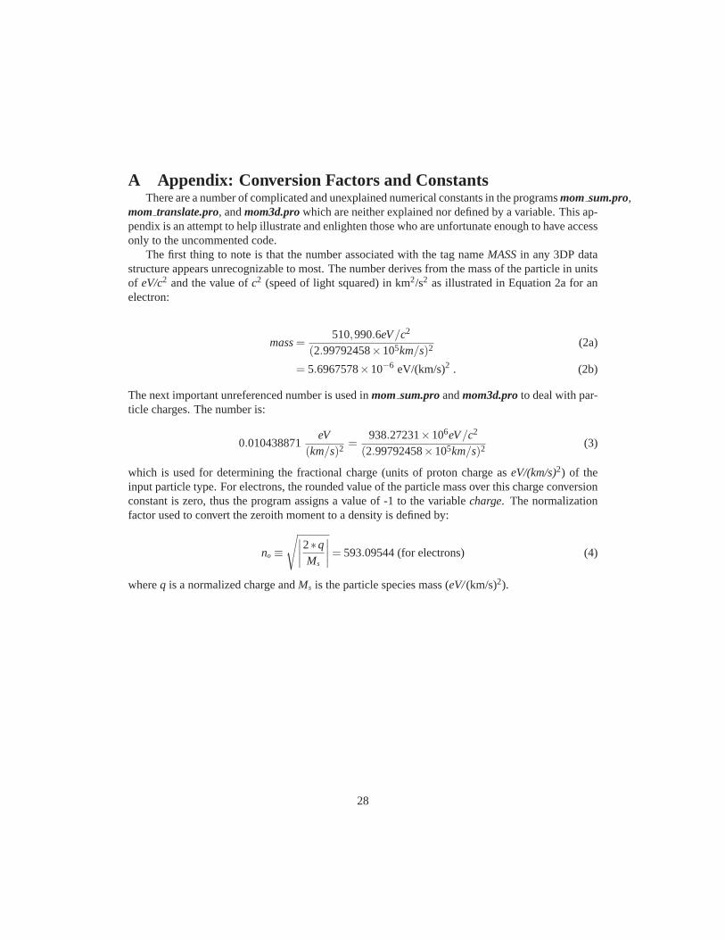
A Appendix: Conversion Factors and ConstantsThere are a number of complicated and unexplained numericalconstants in the programsmom sum.pro,

mom translate.pro, andmom3d.prowhich are neither explained nor defined by a variable. This ap-pendix is an attempt to help illustrate and enlighten those who are unfortunate enough to have accessonly to the uncommented code.

The first thing to note is that the number associated with the tag nameMASSin any 3DP datastructure appears unrecognizable to most. The number derives from the mass of the particle in unitsof eV/c2 and the value ofc2 (speed of light squared) in km2/s2 as illustrated in Equation 2a for anelectron:

mass=510,990.6eV/c2

(2.99792458×105km/s)2 (2a)

= 5.6967578×10−6 eV/(km/s)2 . (2b)

The next important unreferenced number is used inmom sum.proandmom3d.proto deal with par-ticle charges. The number is:

0.010438871eV

(km/s)2 =938.27231×106eV/c2

(2.99792458×105km/s)2 (3)

which is used for determining the fractional charge (units of proton charge aseV/(km/s)2) of theinput particle type. For electrons, the rounded value of theparticle mass over this charge conversionconstant is zero, thus the program assigns a value of -1 to thevariablecharge. The normalizationfactor used to convert the zeroith moment to a density is defined by:

no ≡

√

∣

∣

∣

∣

2∗qMs

∣

∣

∣

∣

= 593.09544 (for electrons) (4)

whereq is a normalized charge andMs is the particle species mass (eV/(km/s)2).

28

ReferencesAptekar, R. L., et al. (1995), Konus-W Gamma-Ray Burst Experiment for the GGS Wind Spacecraft,

Space Science Reviews, 71, 265–272, doi:10.1007/BF00751332.

Bougeret, J.-L., et al. (1995), Waves: The Radio and Plasma Wave Investigation on the Wind Space-craft,Space Science Reviews, 71, 231–263, doi:10.1007/BF00751331.

Desch, M. (2005), Wind: Understanding Interplanetary Dynamics, nASA Goddard Space FlightCenter, Online:http://istp.gsfc.nasa.gov/wind.shtml.

Ergun, R. E., et al. (1998), Wind Spacecraft Observations ofSolar Impulsive Electron Events Asso-ciated with Solar Type III Radio Bursts,Astrophys. J., 503, 435–+, doi:10.1086/305954.

Feldman, W. C., R. C. Anderson, S. J. Bame, S. P. Gary, J. T. Gosling, D. J. McComas, M. F.Thomsen, G. Paschmann, and M. M. Hoppe (1983), Electron velocity distributions near the earth’sbow shock,J. Geophys. Res., 88, 96–110, doi:10.1029/JA088iA01p00096.

Gloeckler, G., et al. (1995), The Solar Wind and Suprathermal Ion Composition Investigation on theWind Spacecraft,Space Science Reviews, 71, 79–124, doi:10.1007/BF00751327.

Kasper, J. C. (2007), Interplanetary Shock Database, harvard-Smithsonian Center for Astrophysics,Online: http://www.cfa.harvard.edu/shocks/.

Lepping, R. P., et al. (1995), The Wind Magnetic Field Investigation, Space Science Reviews, 71,207–229, doi:10.1007/BF00751330.

Lin, R. P., et al. (1995), A Three-Dimensional Plasma and Energetic Particle Investigation for theWind Spacecraft,Space Science Reviews, 71, 125–153, doi:10.1007/BF00751328.

McFadden, J. P., et al. (2007), In-Flight Instrument Calibration and Performance Verification,ISSISci. Rep. Ser., 7, 277–385.

Ogilvie, K. W., et al. (1995), SWE, A Comprehensive Plasma Instrument for the Wind Spacecraft,Space Sci. Rev., 71, 55–77, doi:10.1007/BF00751326.

Owens, A., et al. (1995), A High-Resolution GE Spectrometerfor Gamma-Ray Burst Astronomy,Space Science Reviews, 71, 273–296, doi:10.1007/BF00751333.

Wuest, M., D. S. Evans, and R. von Steiger (2007),Calibration of Particle Instruments in SpacePhysics.

29