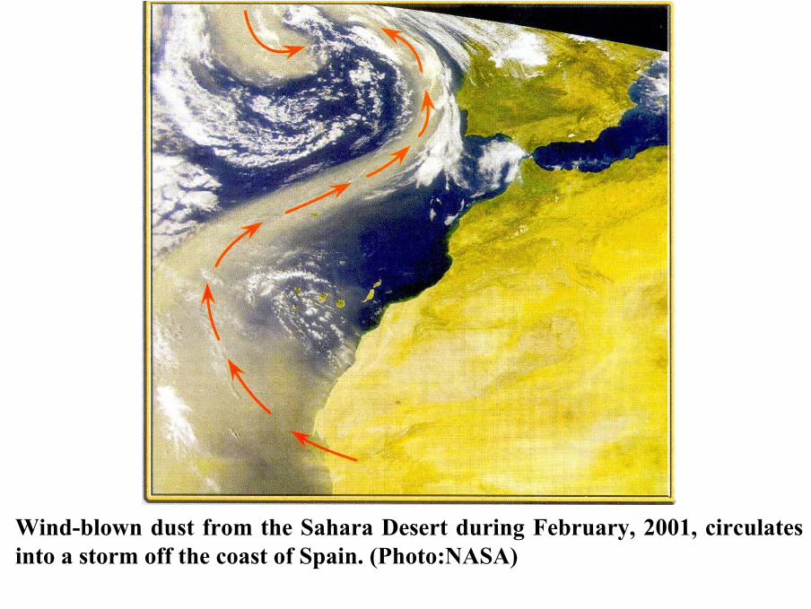
Wind-blown dust from the Sahara Desert during February, 2001, circulatesinto a storm off the coast of Spain. (Photo:NASA)

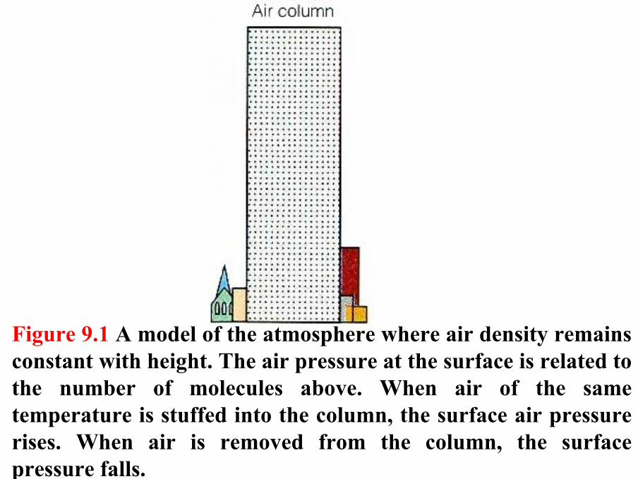
Figure 9.1 A model of the atmosphere where air density remainsconstant with height. The air pressure at the surface is related to the number of molecules above. When air of the sametemperature is stuffed into the column, the surface air pressurerises. When air is removed from the column, the surfacepressure falls.

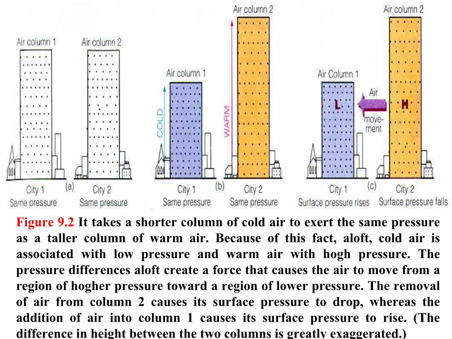
Figure 9.2 It takes a shorter column of cold air to exert the same pressureas a taller column of warm air. Because of this fact, aloft, cold air is associated with low pressure and warm air with hogh pressure. Thepressure differences aloft create a force that causes the air to move from a region of hogher pressure toward a region of lower pressure. The removalof air from column 2 causes its surface pressure to drop, whereas theaddition of air into column 1 causes its surface pressure to rise. (Thedifference in height between the two columns is greatly exaggerated.)

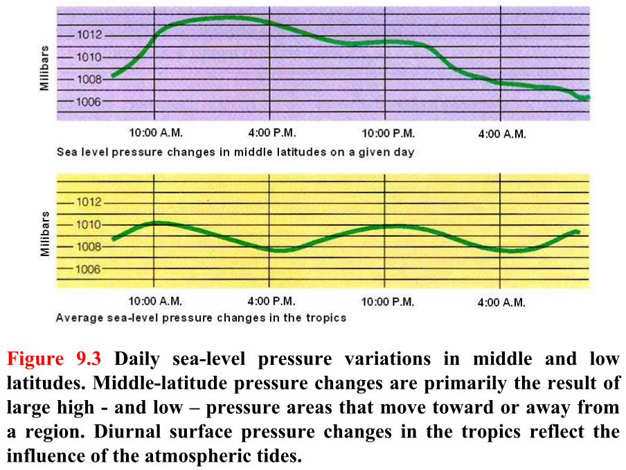
Figure 9.3 Daily sea-level pressure variations in middle and lowlatitudes. Middle-latitude pressure changes are primarily the result oflarge high - and low – pressure areas that move toward or away froma region. Diurnal surface pressure changes in the tropics reflect theinfluence of the atmospheric tides.

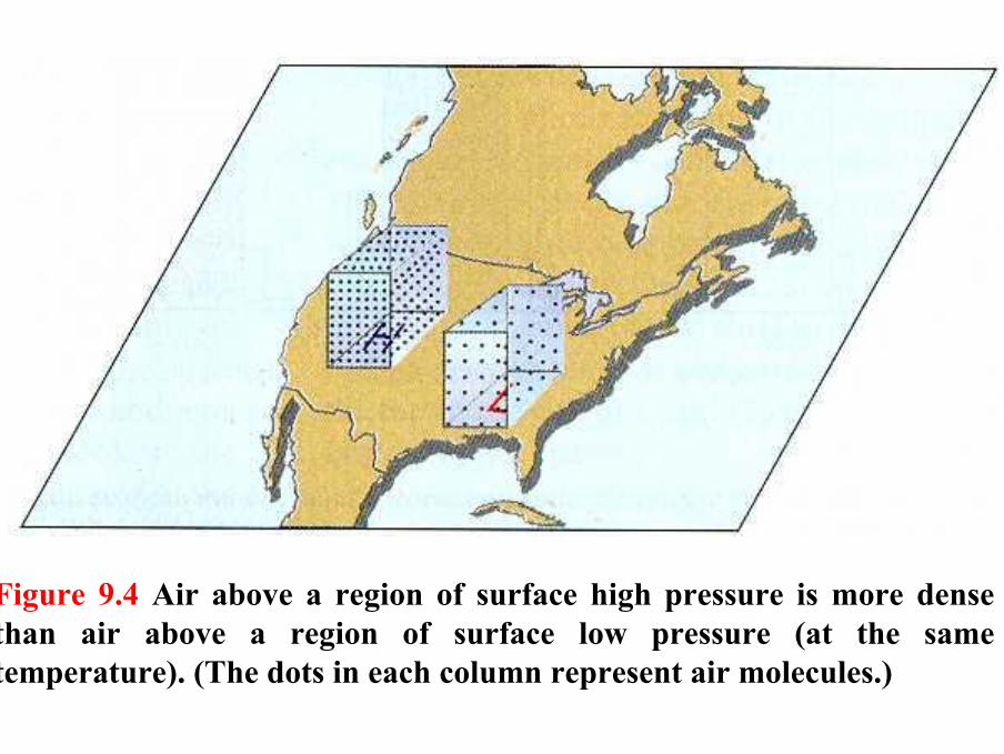
Figure 9.4 Air above a region of surface high pressure is more densethan air above a region of surface low pressure (at the sametemperature). (The dots in each column represent air molecules.)

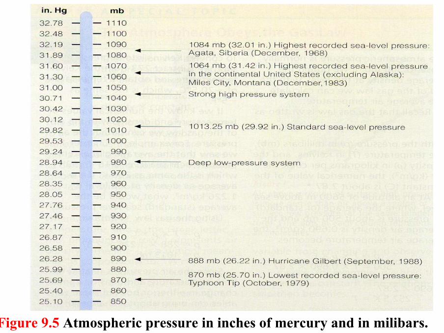
Figure 9.5 Atmospheric pressure in inches of mercury and in milibars.

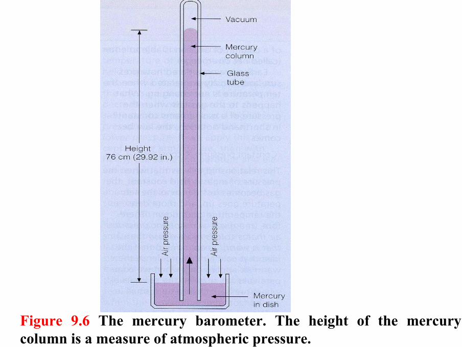
Figure 9.6 The mercury barometer. The height of the mercurycolumn is a measure of atmospheric pressure.

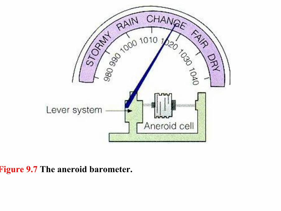
Figure 9.7 The aneroid barometer.

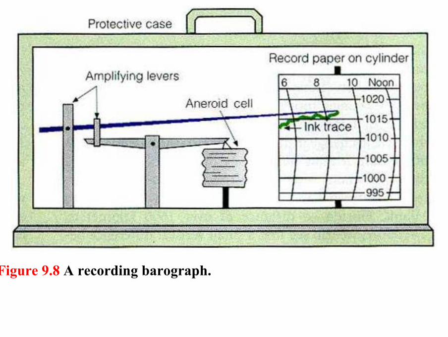
Figure 9.8 A recording barograph.

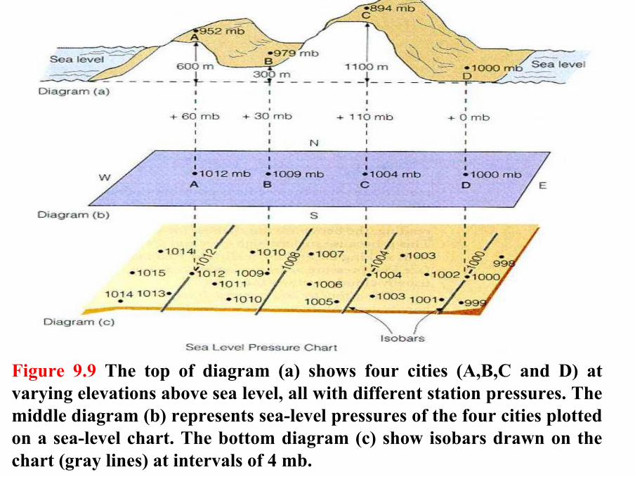
Figure 9.9 The top of diagram (a) shows four cities (A,B,C and D) atvarying elevations above sea level, all with different station pressures. Themiddle diagram (b) represents sea-level pressures of the four cities plottedon a sea-level chart. The bottom diagram (c) show isobars drawn on thechart (gray lines) at intervals of 4 mb.

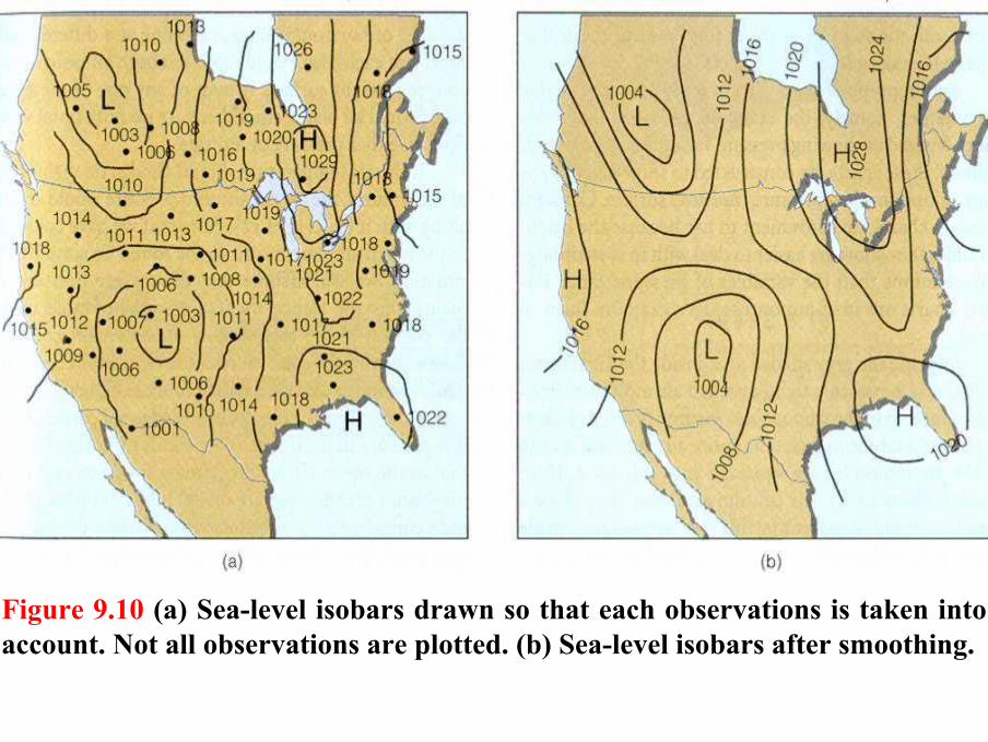
Figure 9.10 (a) Sea-level isobars drawn so that each observations is taken intoaccount. Not all observations are plotted. (b) Sea-level isobars after smoothing.

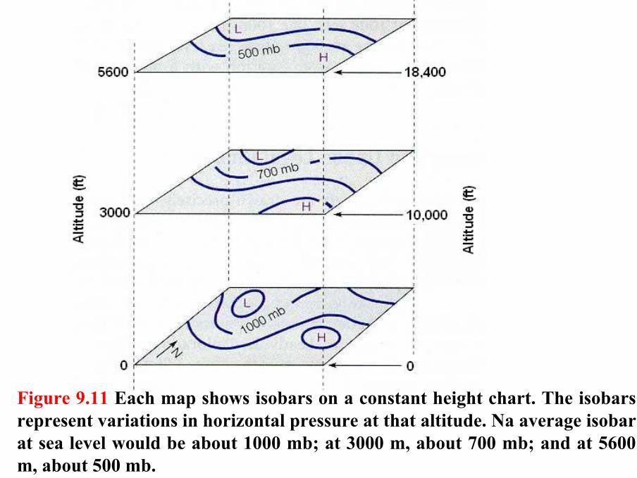
Figure 9.11 Each map shows isobars on a constant height chart. The isobarsrepresent variations in horizontal pressure at that altitude. Na average isobarat sea level would be about 1000 mb; at 3000 m, about 700 mb; and at 5600 m, about 500 mb.

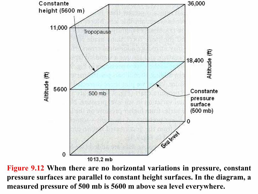
Figure 9.12 When there are no horizontal variations in pressure, constantpressure surfaces are parallel to constant height surfaces. In the diagram, a measured pressure of 500 mb is 5600 m above sea level everywhere.

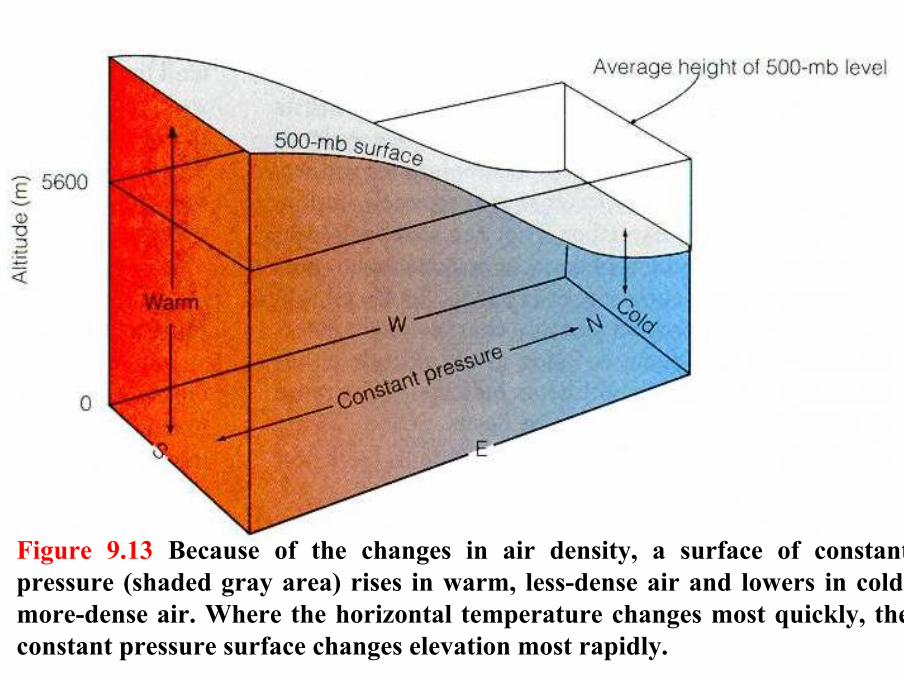
Figure 9.13 Because of the changes in air density, a surface of constantpressure (shaded gray area) rises in warm, less-dense air and lowers in cold, more-dense air. Where the horizontal temperature changes most quickly, theconstant pressure surface changes elevation most rapidly.

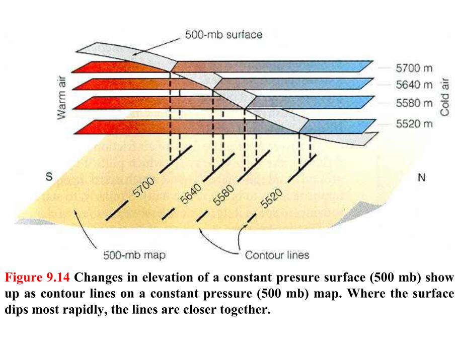
Figure 9.14 Changes in elevation of a constant presure surface (500 mb) show up as contour lines on a constant pressure (500 mb) map. Where the surfacedips most rapidly, the lines are closer together.

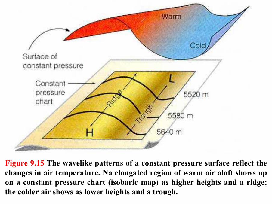
Figure 9.15 The wavelike patterns of a constant pressure surface reflect thechanges in air temperature. Na elongated region of warm air aloft shows upon a constant pressure chart (isobaric map) as higher heights and a ridge; the colder air shows as lower heights and a trough.

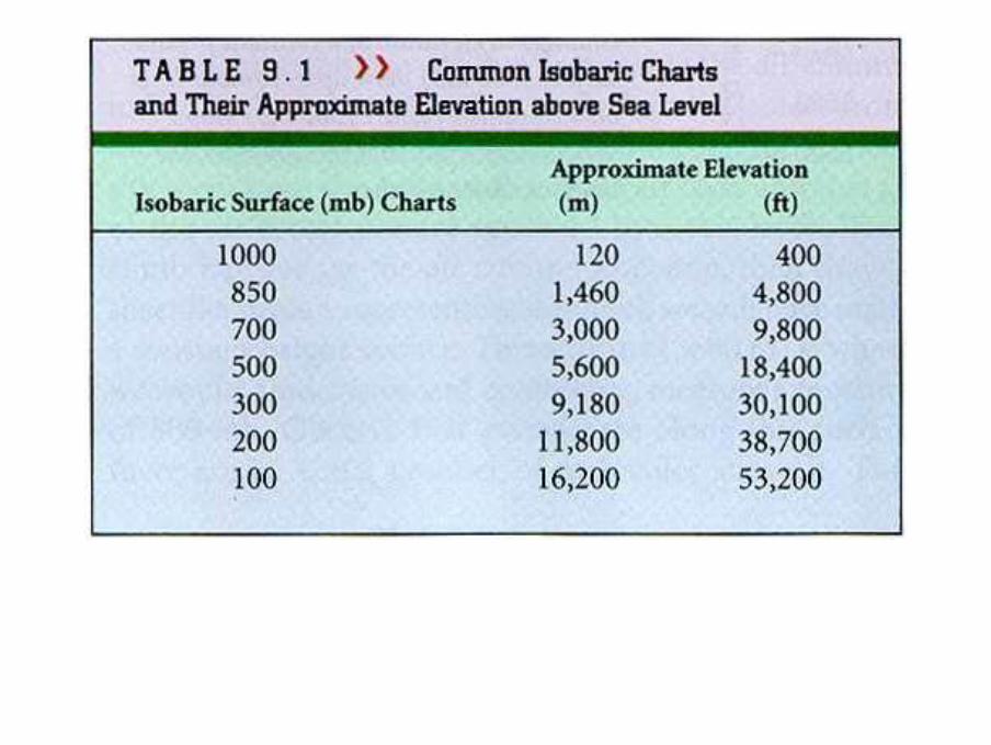
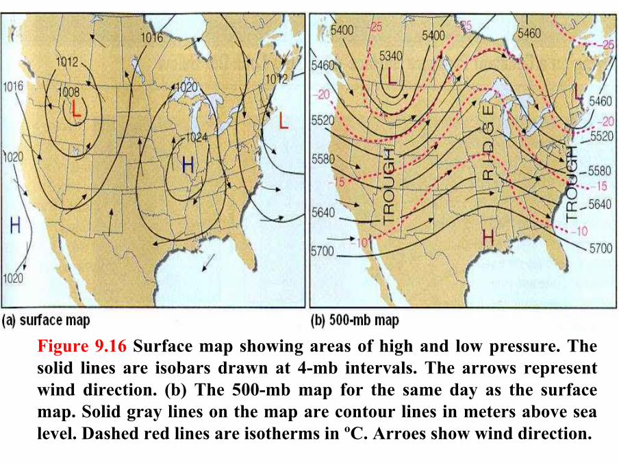
Figure 9.16 Surface map showing areas of high and low pressure. Thesolid lines are isobars drawn at 4-mb intervals. The arrows representwind direction. (b) The 500-mb map for the same day as the surfacemap. Solid gray lines on the map are contour lines in meters above sealevel. Dashed red lines are isotherms in ºC. Arroes show wind direction.

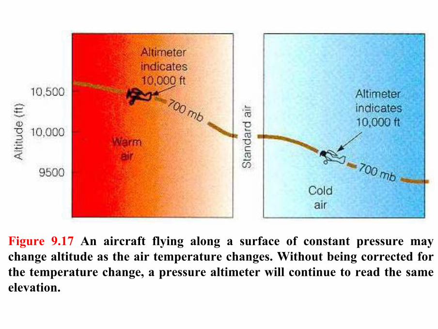
Figure 9.17 An aircraft flying along a surface of constant pressure maychange altitude as the air temperature changes. Without being corrected for the temperature change, a pressure altimeter will continue to read the sameelevation.

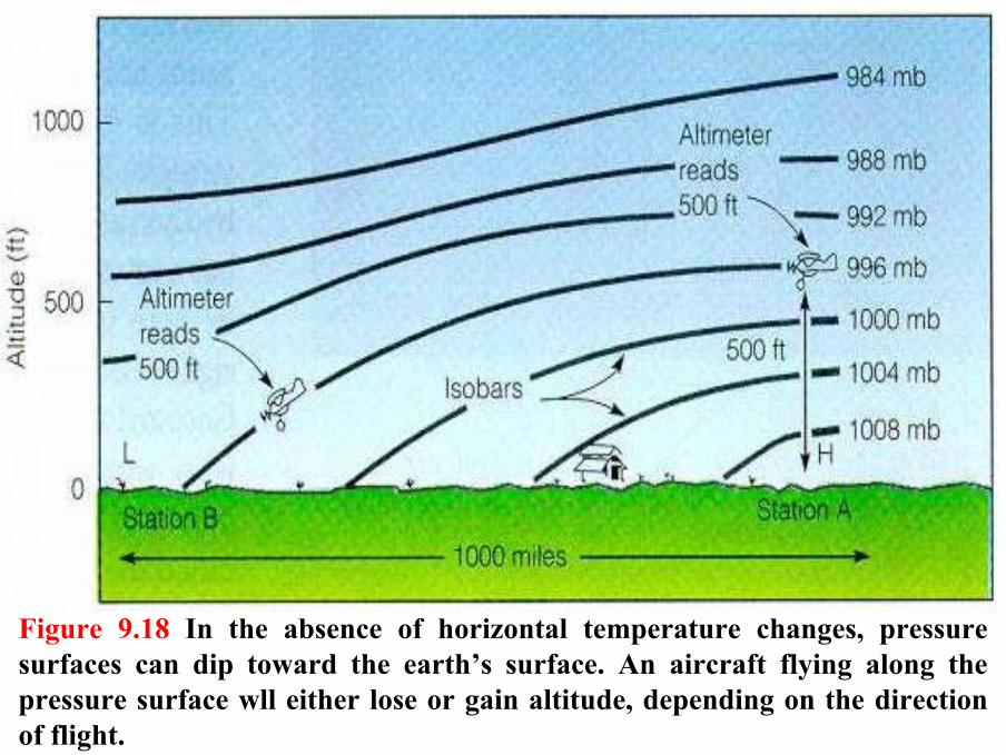
Figure 9.18 In the absence of horizontal temperature changes, pressuresurfaces can dip toward the earth’s surface. An aircraft flying along thepressure surface wll either lose or gain altitude, depending on the directionof flight.

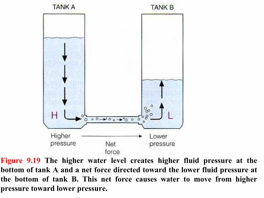
Figure 9.19 The higher water level creates higher fluid pressure at thebottom of tank A and a net force directed toward the lower fluid pressure atthe bottom of tank B. This net force causes water to move from higherpressure toward lower pressure.

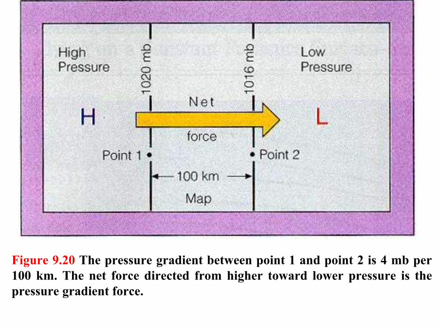
Figure 9.20 The pressure gradient between point 1 and point 2 is 4 mb per 100 km. The net force directed from higher toward lower pressure is thepressure gradient force.

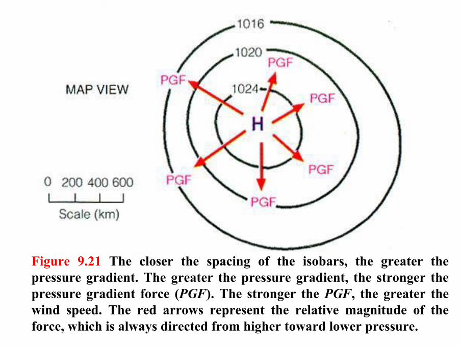
Figure 9.21 The closer the spacing of the isobars, the greater thepressure gradient. The greater the pressure gradient, the stronger thepressure gradient force (PGF). The stronger the PGF, the greater thewind speed. The red arrows represent the relative magnitude of theforce, which is always directed from higher toward lower pressure.

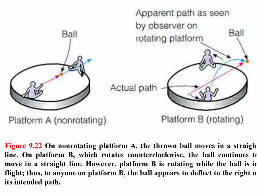
Figure 9.22 On nonrotating platform A, the thrown ball moves in a straightline. On platform B, which rotates counterclockwise, the ball continues to move in a straight line. However, platform B is rotating while the ball is in flight; thus, to anyone on platform B, the ball appears to deflect to the right ofits intended path.

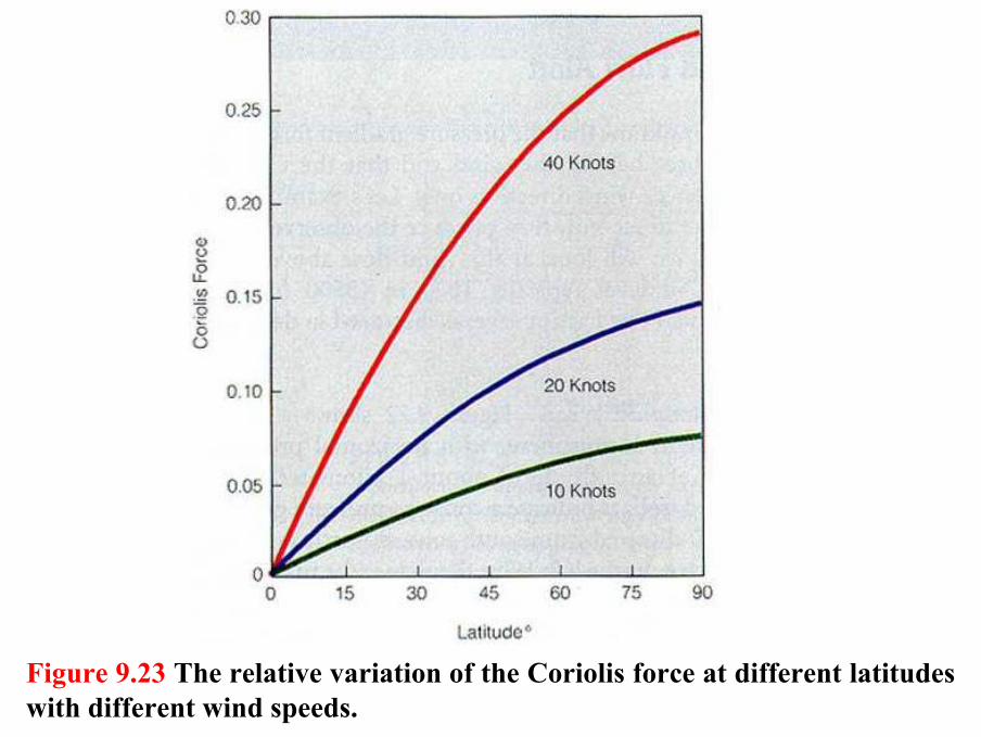
Figure 9.23 The relative variation of the Coriolis force at different latitudes with different wind speeds.

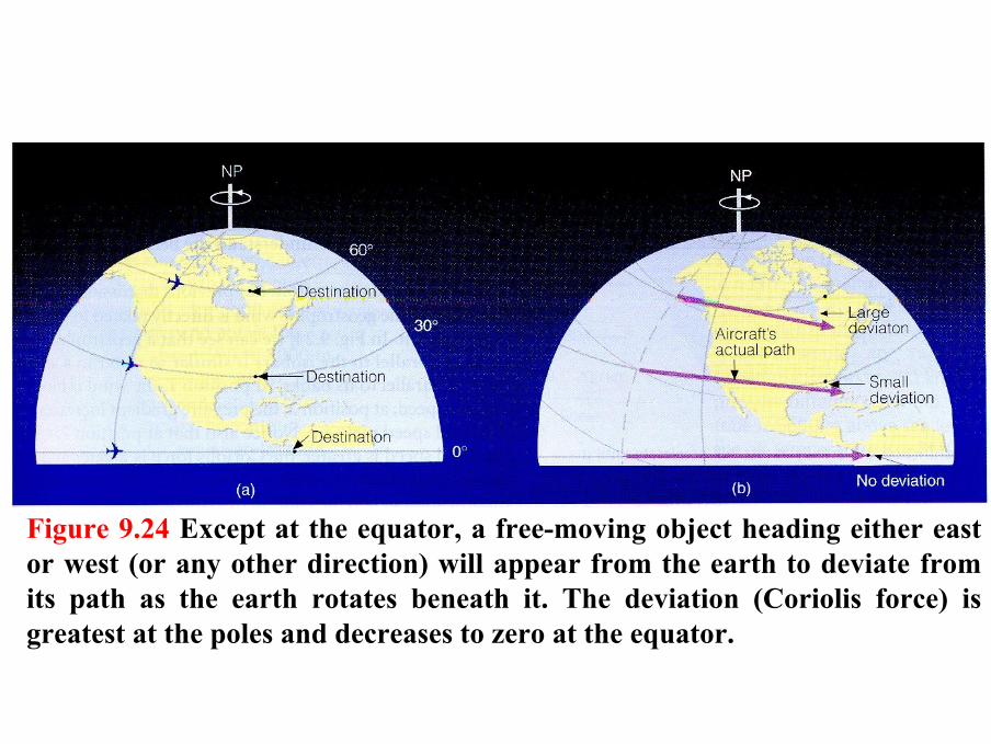
Figure 9.24 Except at the equator, a free-moving object heading either eastor west (or any other direction) will appear from the earth to deviate fromits path as the earth rotates beneath it. The deviation (Coriolis force) is greatest at the poles and decreases to zero at the equator.

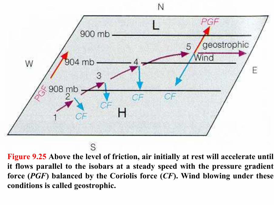
Figure 9.25 Above the level of friction, air initially at rest will accelerate untilit flows parallel to the isobars at a steady speed with the pressure gradientforce (PGF) balanced by the Coriolis force (CF). Wind blowing under theseconditions is called geostrophic.

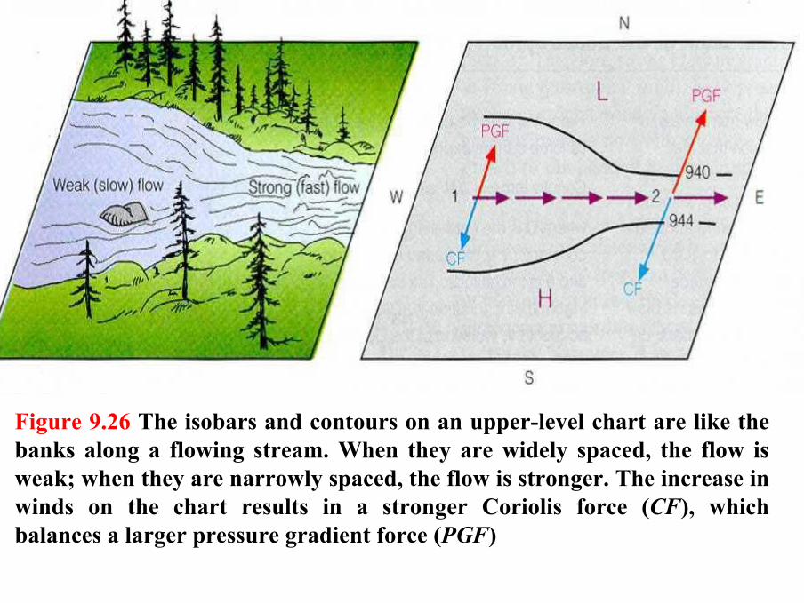
Figure 9.26 The isobars and contours on an upper-level chart are like thebanks along a flowing stream. When they are widely spaced, the flow is weak; when they are narrowly spaced, the flow is stronger. The increase in winds on the chart results in a stronger Coriolis force (CF), whichbalances a larger pressure gradient force (PGF)

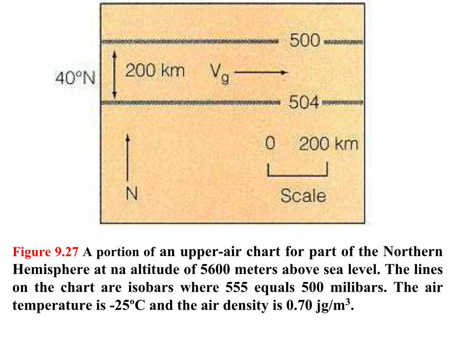
Figure 9.27 A portion of an upper-air chart for part of the NorthernHemisphere at na altitude of 5600 meters above sea level. The lineson the chart are isobars where 555 equals 500 milibars. The airtemperature is -25ºC and the air density is 0.70 jg/m3.

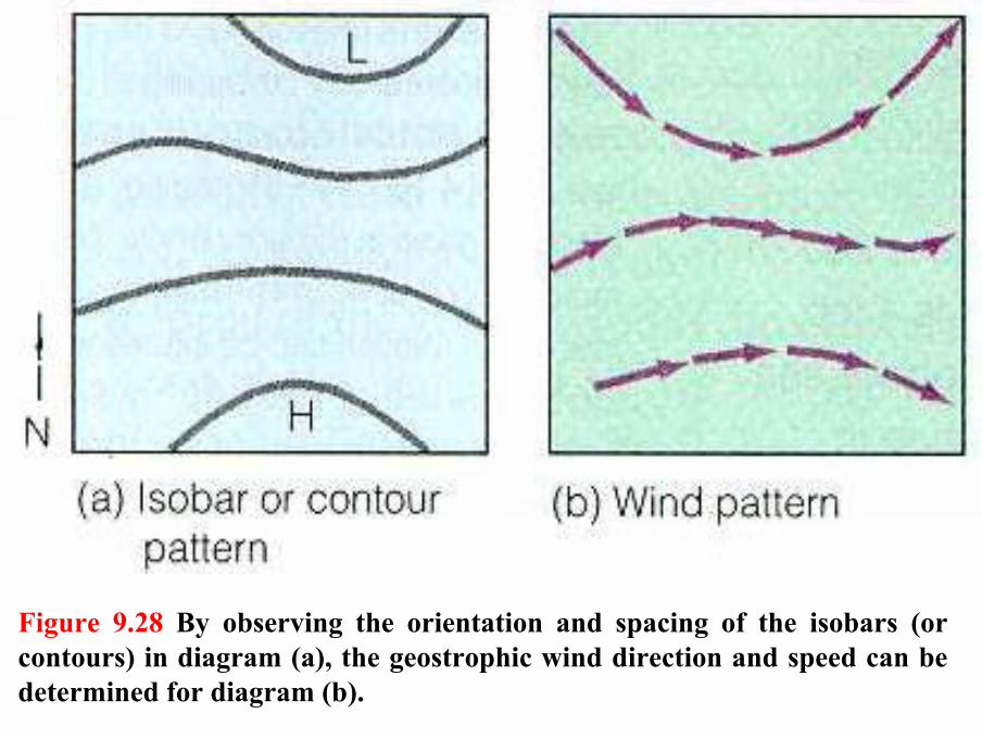
Figure 9.28 By observing the orientation and spacing of the isobars (orcontours) in diagram (a), the geostrophic wind direction and speed can bedetermined for diagram (b).

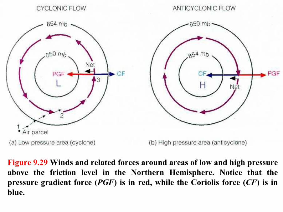
Figure 9.29 Winds and related forces around areas of low and high pressureabove the friction level in the Northern Hemisphere. Notice that thepressure gradient force (PGF) is in red, while the Coriolis force (CF) is in blue.

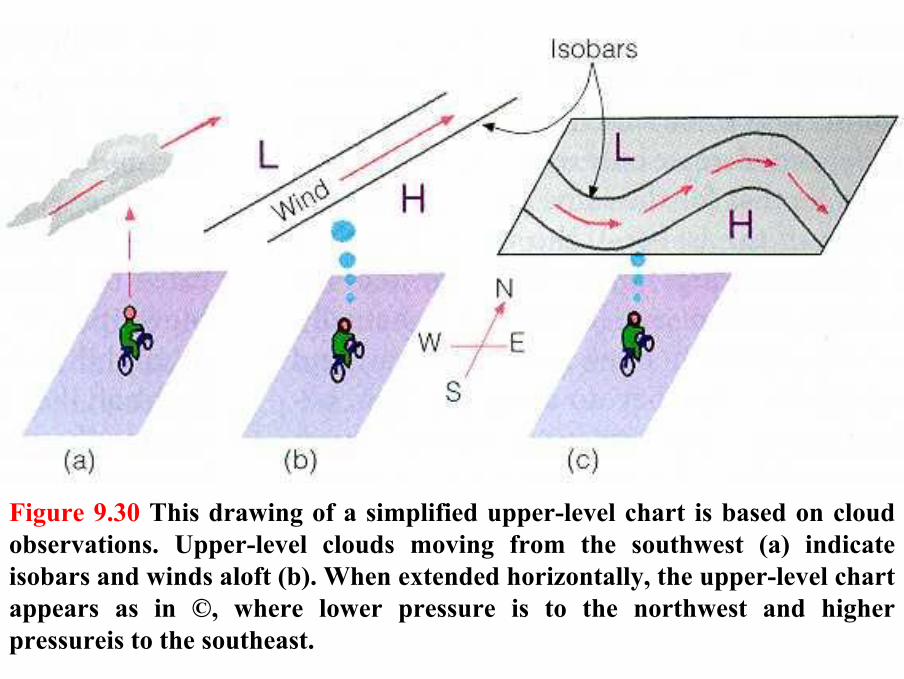
Figure 9.30 This drawing of a simplified upper-level chart is based on cloudobservations. Upper-level clouds moving from the southwest (a) indicateisobars and winds aloft (b). When extended horizontally, the upper-level chartappears as in ©, where lower pressure is to the northwest and higherpressureis to the southeast.

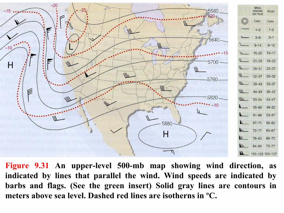
Figure 9.31 An upper-level 500-mb map showing wind direction, as indicated by lines that parallel the wind. Wind speeds are indicated bybarbs and flags. (See the green insert) Solid gray lines are contours in meters above sea level. Dashed red lines are isotherns in ºC.

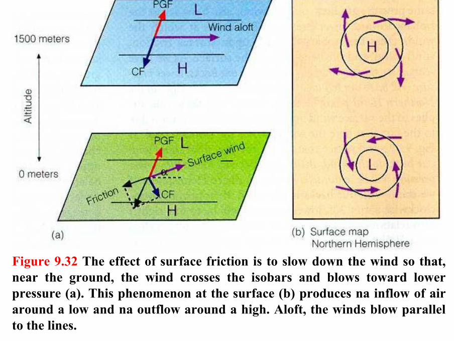
Figure 9.32 The effect of surface friction is to slow down the wind so that, near the ground, the wind crosses the isobars and blows toward lowerpressure (a). This phenomenon at the surface (b) produces na inflow of airaround a low and na outflow around a high. Aloft, the winds blow parallelto the lines.

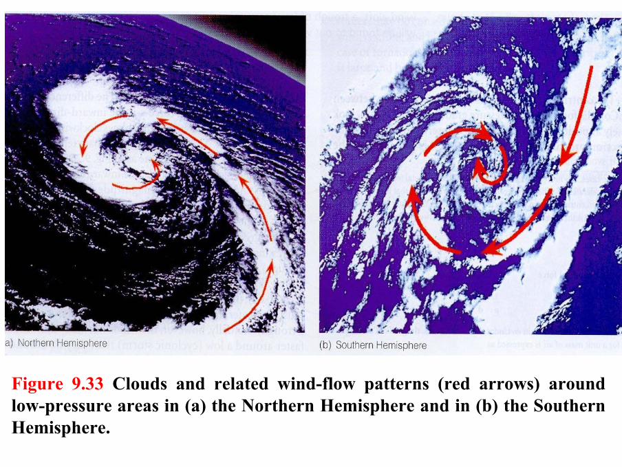
Figure 9.33 Clouds and related wind-flow patterns (red arrows) aroundlow-pressure areas in (a) the Northern Hemisphere and in (b) the SouthernHemisphere.

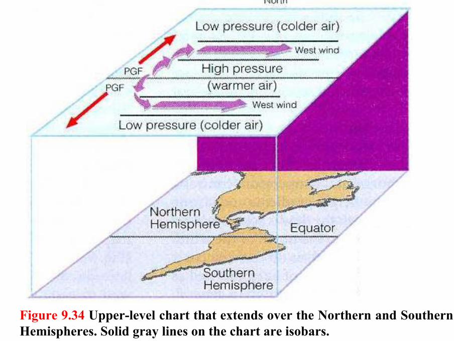
Figure 9.34 Upper-level chart that extends over the Northern and SouthernHemispheres. Solid gray lines on the chart are isobars.

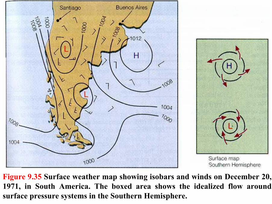
Figure 9.35 Surface weather map showing isobars and winds on December 20, 1971, in South America. The boxed area shows the idealized flow aroundsurface pressure systems in the Southern Hemisphere.

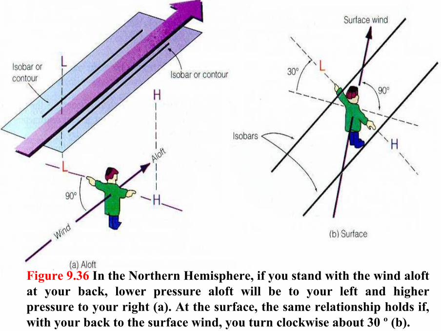
Figure 9.36 In the Northern Hemisphere, if you stand with the wind aloftat your back, lower pressure aloft will be to your left and higherpressure to your right (a). At the surface, the same relationship holds if, with your back to the surface wind, you turn clockwise about 30 º (b).

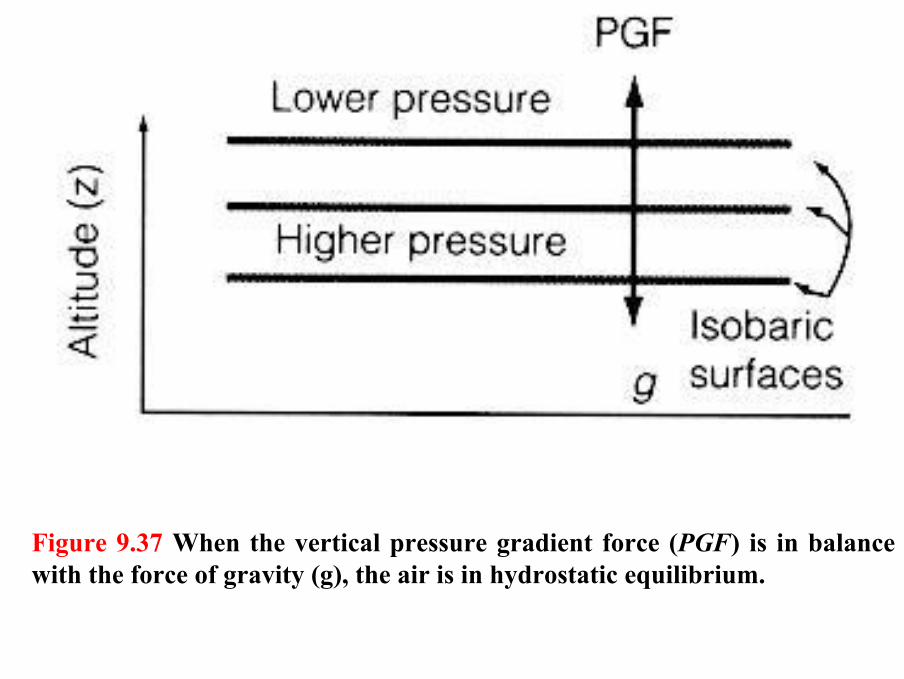
Figure 9.37 When the vertical pressure gradient force (PGF) is in balance with the force of gravity (g), the air is in hydrostatic equilibrium.

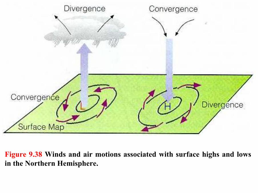
Figure 9.38 Winds and air motions associated with surface highs and lowsin the Northern Hemisphere.