Willingness to Pay for Biodiesel in Diesel Engines: A Stochastic Double Bounded

Contingent Valuation Survey

P. Wilner Jeanty*, Tim Haab**, and Fred Hitzhusen**

Selected paper prepared for presentation at the American Agricultural Economics

Association Annual Meeting, Portland, Oregon, July 23-26, 2007

The double bounded dichotomous choice format has been proven to improve efficiency in

contingent valuation models. However, this format has been criticized due to lack of

behavioral and statistical consistencies between the first and the second responses. In this

study a split sampling methodology was used to determine whether allowing respondents to

express uncertainty in the follow-up question would alleviate such inconsistencies. Results

indicate that allowing respondents to express uncertainty in the follow-up question was

effective at reducing both types of inconsistencies while efficiency gain is maintained.

Keywords: Biodiesel, diesel, environmental benefits, contingent valuation, willingness to

pay, double bounded model, and statistical and behavioral inconsistencies.

JEL Classification: I18, L91, Q42, Q51, Q53

Copyright 2006 by P. Wilner Jeanty, Tim Haab, and Fred Hitzhusen. All rights reserved.

Readers may make verbatim copies of this document for non-commercial purposes by any

means, provided that this copyright notice appears on all such copies.

* Post-doctoral researcher and ** Professors, Dept. of Agricultural, Environmental, and

Development Economics, the Ohio State University.

1

In order to elicit individuals’ willingness to pay (WTP) for a non-market good, the National

Oceanic Atmospheric Administration (NOAA) recommends using the dichotomous choice

format in contingent valuation surveys (Arrow et al., 1993). This approach consists of asking

respondents whether they would be willing to pay a particular price for the good. The

prominent advantage of this approach is that it mimics the decision task that individuals face

in everyday life: whether you buy it or not (Carlsson and Johansson-Stenman, 2000). A

significant drawback inherent in this approach, however, is its relatively poor efficiency due

to limited information obtained from each respondent, necessitating the use of fairly large

samples in order to attain a reasonable degree of accuracy in welfare estimates. The double

bounded dichotomous choice (DB-DC) format has emerged as a means to improve statistical

efficiency in contingent valuation applications. Recent work includes Loureiro et al., (2006),

Yoo and Chae (2001), Calia and Strezzera (2000), and McLeod and Bergland (1999). The

double bounded approach, first developed by Hanemann et al. (1991), entails asking the

respondent two yes/no WTP questions where the bid price in the second or follow-up

question is higher (respectively lower) if the answer to first question is positive (respectively

negative). However, this approach has been criticized due to statistical and behavioral

inconsistencies observed between the first and the second responses. (Bateman et al., 2001;

Harrison and Kristöm, 1995).

Despite this potential for bias, the use of the double bounded question format seems to be

justified since it leads to lower mean squared error (Alberini, 1995) or yields a more

conservative WTP estimate (Banzhaf et al., 2004) by narrowing down the confidence interval

around WTP measures. One way to avert strategic behavior associated with the double

bounded format while gaining efficiency is to adopt a “one and one half” bound model

2

suggested by Cooper, Hanemann, and Signorelli (2002). However, Bateman et al. (2006)

show that this model fails crucial tests of procedural invariance and induces strategic

behavior among responses as in the double bounded model. In this current study, focusing on

the follow-up question, we seek to determine whether allowing respondents to express

uncertainty in the double bounded dichotomous choice format has an effect in reducing the

strategic behavior (downward mean shift) and statistical inconsistency (imperfect correlation)

while efficiency gain is maintained.

In a contingent valuation survey to estimate WTP for using more biodiesel fuel in diesel

engines in a 16 county airshed in Central and South Eastern Ohio, a split sampling

methodology was used wherein the first half respondents received questionnaires with the

conventional DB-DC format and the second half respondents received questionnaires in

which the follow-up question is in a stochastic format. Unlike the conventional follow-up

question which requires a yes/no answer from a respondent, the stochastic follow-up question

asks the respondent for the probability or likelihood of paying a higher (respectively lower)

bid amount if he/she answers “yes” (respectively “no”) to the first WTP question. Answer

choices for the stochastic follow-up question include “Definitely no”, “Probably no”, “Not

sure”, “Probably yes”, and “Definitely yes”. Numeric answers ranging from 0 to 100 were

also offered to support the verbal answer choices. From a methodological standpoint, this

study distinguishes from previous research by being the first to implement a double bounded

contingent valuation survey with a stochastic follow-up question.

To compare the dichotomous choice format with the conventional follow-up question to a

dichotomous choice format with the proposed stochastic follow-up question, uncertain

response choices were recoded in yes/no answers, allowing estimation of several bivariate

3

probit models. Results indicate that the stochastic follow-up approach performs better than

the conventional follow-up format in terms of efficiency. The estimated error correlation

coefficients in models using the stochastic follow-up data are higher, reducing statistical

inconsistency between the first and second responses. The stochastic double bounded format

yields models for which mean WTP in both questions are not only the same but more

efficient than those in the single bounded format.

This article is organized as follows. The next section reviews the literature on uncertainty

in contingent valuation models and explains the rationale behind the stochastic format.

Section 3 briefly describes the survey methodology. Section 4 outlines the model

specification and estimation procedures. The empirical results of the analysis are presented in

section 5. Section 6 concludes the study and presents areas for further research.

Uncertainty in Contingent Survey and the Stochastic Double Bounded Approach

The notion of preference uncertainty from the perspective of the respondents has been

investigated by a number of studies. According to Li and Mattsson (1995), under preference

uncertainty, it is possible for some individuals to answer yes even if their true valuation is

less than the bid or no even if their true valuation is greater than the bid. Consequently, Li

and Masson (1995) model the individual’s yes/no choice as a specific realization of some

underlying probabilistic mechanism. In addition to the discrete choice question on whether to

pay a given bid for the resource, a post-decisional confidence measure was elicited using a

follow-up debriefing question in which they design a graphical scale from 0 to 100% with

5% intervals. These measures are then interpreted as subjective probabilities that the

individual’s valuation is greater (for a yes answer) or less (for a no answer) than the bid.

4

Similar to Li and Mattsson, Loomis and Ekstrand (1998) use a debriefing question after

the dichotomous choice question. The question wording is as follows:

On a scale of 1 to 10, how certain are you of your answer to the previous question?

Please circle the number that best represents your answer if 1=not certain and

10=very certain.

It was found that 45 percent of the respondents giving “no” responses were very certain

of their answers, while only 30 percent of those giving “yes” responses were equally certain.

Welsh and Poe (1998) develop a multiple bounded question format with uncertain

response options. The difference between the single and double bounded formats and the

multiple bounded format is that the latter lists a number of bids and respondents are asked

whether they would pay each bid amount. Alberini et al. (2003) expand on Welsh and Poe to

devise a conceptual model supporting the use of uncertainty response options. However,

these studies yield divergent results, indicating that more needs to be done in terms of

framing of the questions and response formats. This need gives motivation for an attempt to

incorporate uncertainty in the double bounded question format by focusing on the follow-up

question, which bears the brunt of the double bounded model’s criticism.

A more recent study by Vassanadumrongdee and Matsuoka (2005) has attempted to take

into account uncertainty in a contingent valuation with a follow-up question. Their study

focused on measuring individuals’ willingness to pay (WTP) to reduce mortality risk arising

from air pollution and traffic accidents in Bangkok, Thailand. In the final section of their

questionnaire, two debriefing questions were asked, the first of which was to capture the

degree of certainty about the WTP responses. The respondents were asked how confident

they were about their answers to both the first and second WTP questions. Only 28 percent in

5

the air pollution sample and 24 percent in the traffic accident sample reported that they were

very confident about their WTP answers.

In this current study, a different methodology is used to incorporate uncertainty in CVM.

Unlike these studies mentioned above, the focus is on double bounded dichotomous choice

approach. We argue that the inconsistency observed between the first and the second

responses may be due to uncertainty created when the second question is introduced.

Therefore, allowing respondents to express uncertainty in the second responses may help

alleviate this inconsistency problem.

The first dichotomous choice question is more market-like and often considered more

similar to every day consumption decisions, i.e. you either buy or do not buy the good at a

certain price (Carlsson and Johansson-Stenman, 2000). Before the second question arrives, it

is possible that respondents know their valuation with certainty under certain conditions such

as some prior knowledge of the good or service. However, the follow-up question may result

in creating uncertainties about the nature and the quality of the good or service. Respondents

may follow decision rules not reflecting their true valuation, since neither a ‘yes’ nor a “no”

could accurately convey their true preferences. Since confining and restrictive, it renders the

respondents’ task difficult.

An elicitation format designed to ease the respondents’ burden is presented as an

alternative to the current DB-DC format. After the first question, the stochastic double

bounded format asks respondents the likelihood that they would vote for the project

regardless of their decision on the first dichotomous choice question. Since this alternative

approach calls for an answer in a likelihood format in the second round, it is referred to as the

stochastic or random double-bounded format.

6

Survey methodology

Between May and June 2006, 3500 survey questionnaires were mailed out to a random

sample of residents aged 18 years or older in two Ohio regions: Southeastern and Central

Ohio. One half of the respondents received questionnaires with a conventional follow-up

question and to the other half, questionnaires with a stochastic follow-up question were sent

(See both follow-up formats in the Appendix). However, inherent in the stochastic follow-up

were two important issues. First, different people would give divergent interpretations to the

verbal answer choices. Thus, numeric answers ranging from 0 to 100 were offered to support

the verbal answer choices. Second, order effects may arise depending on whether the

subjective probabilities are presented in ascending or descending order. An example of order

effect is primacy effect, which is a tendency of a respondent to choose items that appear first

in a list. In order to test for order effect, the second half of the survey sample was subdivided.

One portion of respondents received questionnaires wherein the order of the response choices

was “Definitely no”, “Probably no”, “Not sure”, “Probably yes”, and “Definitely yes”. The

order was reversed for the other portion.

Based on results of a pre-test, the sets of bids used in the study were: (50, 25, 100), (75,

40, 150), (100, 50, 200), and (250, 125, 500) where the first element of each set represents

the first bid, the second element corresponds to the lower bid if the respondent answers “no”

to the first bid, and the third element corresponds to the higher bid if the response to the first

bid is a “yes”. The payment vehicle used was a one time lump sum contribution to a trust

fund designed for a biodiesel project. To minimize non-response bias, we followed

procedures suggested in Dillman (2000) when implementing the survey.

7

The survey questionnaire was split into four sections. The first section dealt with the

respondents’ background on air pollution in general and on global environmental changes

and with their attitude toward diesel, biodiesel, and the environment. The second section

contained the valuation scenario, which attempted to provide as much information as

possible about the hypothetical market. Guidelines for a valid contingent valuation analysis

suggested by Carson (2000), Carson et al. (2001), and Arrow et al. (1993) were followed as

much as possible. To establish the institutional setting in which the good would be provided,

the respondents were told that the Office of Energy Efficiency at the Ohio Department of

Development is considering a project to reduce air pollution emissions in their county using

B20, a blend of 20% pure biodiesel and 80% pure diesel. However, consistent with previous

studies (Loureiro et al., 2006), they were not explicitly told whether the results of the study

will affect these considerations. Providing this information to the respondents could have

affected their decisions, given the context in which the good would be provided.

The third part of the questionnaire focused on economic and socio-demographic

characteristics of the respondents. The final section concerned evaluation of the survey. It

checked whether the respondents fully understood what they were asked to value and

whether the information provided in the survey was useful for and relevant to them.

Model Specification and Estimation Procedures

In order to assess the internal validity of the contingent valuation, we first estimate four

single bounded probit and logit models using linear and exponential functional forms. These

models are described in Haab and McConnell (2002). That part of the analysis focuses on the

first dichotomous choice question, and all appropriate covariates are used. Data from the two

8

follow-up approaches are pooled together. Second, for each follow-up approach, a

dichotomous choice (DC) single bounded model and DC double bounded bivariate probit

models are estimated for efficiency and follow-up approach comparison. As in Moran and

Moraes (1999), only the bid price and income are used as covariates. Note that simply

allowing respondents to express uncertainty in the follow up question has nothing to do with

efficiency. However, the central tendency may be affected. Efficiency gain would occur only

if the stochastic follow-up format leads to higher correlation between the first and the second

questions.

We employ bivariate probit for the double bounded models because the bivariate normal

density function is appealing to statisticians in the sense that it allows for non-zero

correlation, while the logistic distribution does not. In addition, constraining the parameters

in the bivariate probit model yields other models such as the interval data model and the

random effects probit model (Cameron and Quiggin, 1994; Haab, 1997). Specifically, when

the correlation coefficient between the error terms of the two questions is relatively high,

more efficient welfare measures can be obtained by constraining the means and the variances

to be equal across questions1.

Econometrically modeling data generated by the double bounded question format relies

on the formulation given by:

WTPij = µi + εij (1)

where WTPij represents the jth respondent’s willingness to pay and i=1,2 denoting the first

and the second question. µ1 and µ2 are the means for the first and the second responses.

Setting µij = X’ijβi allows the means to be dependent upon the characteristics of the

respondents.

9

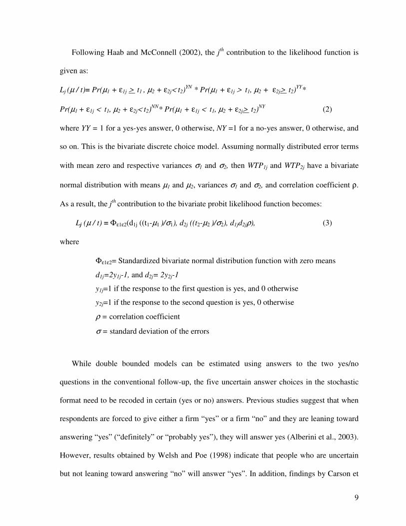
Following Haab and McConnell (2002), the jth contribution to the likelihood function is

given as:

Lj (µ / t)= Pr(µ1 + ε1j > t1 , µ2 + ε2j< t2)YN

* Pr(µ1 + ε1j > t1, µ2 + ε2j> t2)YY

*

Pr(µ1 + ε1j < t1, µ2 + ε2j< t2)NN

* Pr(µ1 + ε1j < t1, µ2 + ε2j> t2)NY (2)

where YY = 1 for a yes-yes answer, 0 otherwise, NY =1 for a no-yes answer, 0 otherwise, and

so on. This is the bivariate discrete choice model. Assuming normally distributed error terms

with mean zero and respective variances σ1 and σ2, then WTP1j and WTP2j have a bivariate

normal distribution with means µ1 and µ2, variances σ1 and σ2, and correlation coefficient ρ.

As a result, the jth contribution to the bivariate probit likelihood function becomes:

Lj (µ / t) = Φε1ε2(d1j ((t1-µ1 )/σ1), d2j ((t2-µ2 )/σ2), d1jd2jρ), (3)

where

Φε1ε2= Standardized bivariate normal distribution function with zero means

d1j=2y1j-1, and d2j= 2y2j-1

y1j=1 if the response to the first question is yes, and 0 otherwise

y2j=1 if the response to the second question is yes, 0 otherwise

ρ = correlation coefficient

σ = standard deviation of the errors

While double bounded models can be estimated using answers to the two yes/no

questions in the conventional follow-up, the five uncertain answer choices in the stochastic

format need to be recoded in certain (yes or no) answers. Previous studies suggest that when

respondents are forced to give either a firm “yes” or a firm “no” and they are leaning toward

answering “yes” (“definitely” or “probably yes”), they will answer yes (Alberini et al., 2003).

However, results obtained by Welsh and Poe (1998) indicate that people who are uncertain

but not leaning toward answering “no” will answer “yes”. In addition, findings by Carson et

10

al. (1998) imply that all uncertain responses should be no responses in a binary yes/no

response choice. Based on these divergent results, the following recoding methods are used.

First, “definitely” and “probably yes” are recoded as “yes” and all other response choices are

recoded as “no”. Second, “definitely yes”, “probably yes”, and “not sure” are recoded as

“yes” and all others as “no”. A third recoding method, which is in line with the results by

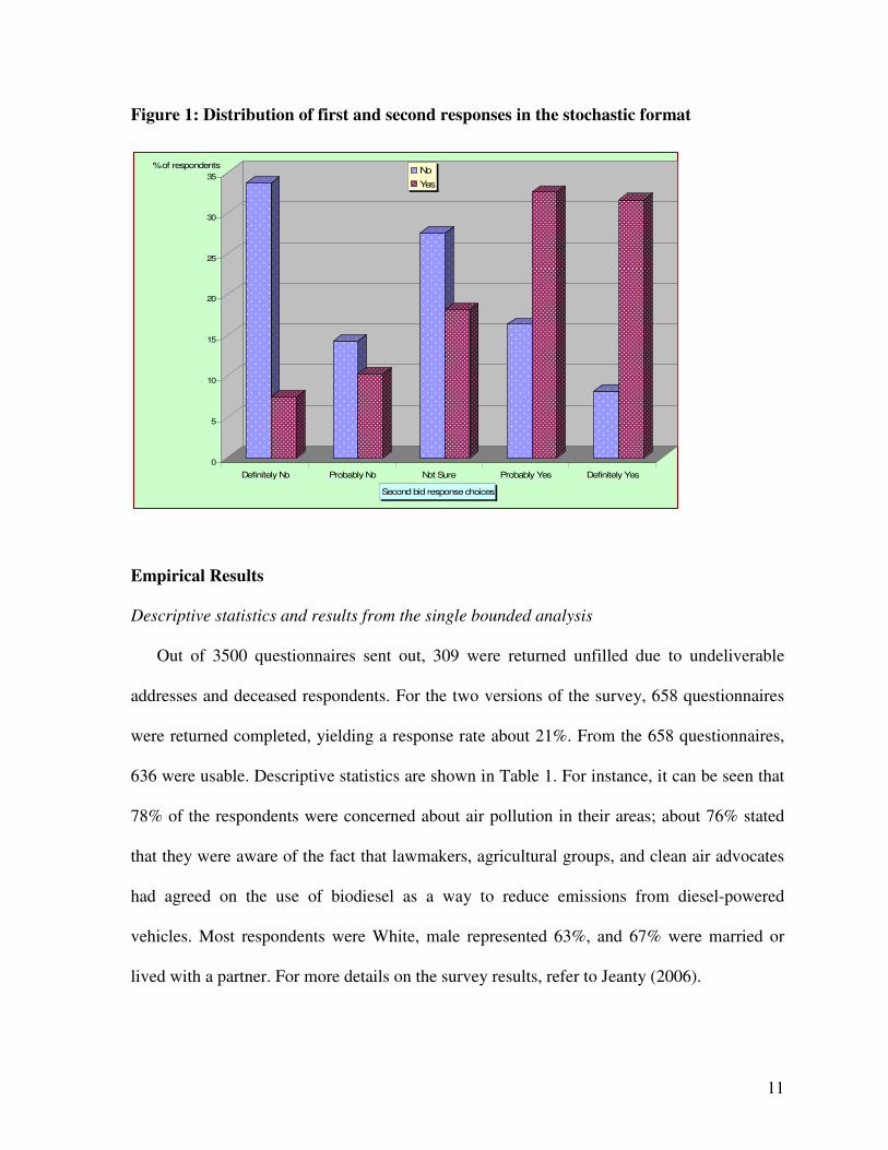
Welsh and Poe (1998), is suggested by the response pattern in the second sub-sample. Figure

1 indicates that respondents who answered “no” to the first WTP question seem to lean

toward answering “no” to the follow-up question. As a result, if they are “not sure” they will

be less likely to answer “yes”. This reasoning yields the third recoding method, which is the

same as the second method except that “not sure” responses are recoded as “yes” only for

those respondents who answered “yes” to the first WTP question. All models2 were estimated

using the maximum likelihood estimation technique. Also, data management and the

empirical analysis were conducted using STATA 9.2.

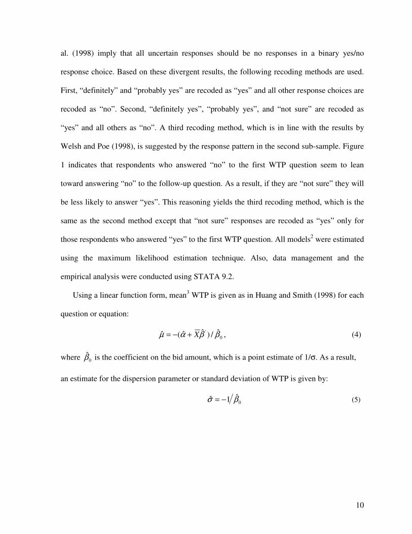
Using a linear function form, mean3 WTP is given as in Huang and Smith (1998) for each

question or equation:

0

' ˆ/)ˆˆ(ˆ ββαµ X+−= , (4)

where 0β̂ is the coefficient on the bid amount, which is a point estimate of 1/σ. As a result,

an estimate for the dispersion parameter or standard deviation of WTP is given by:

0ˆ1ˆ βσ −= (5)

11

Figure 1: Distribution of first and second responses in the stochastic format

Empirical Results Descriptive statistics and results from the single bounded analysis

Out of 3500 questionnaires sent out, 309 were returned unfilled due to undeliverable

addresses and deceased respondents. For the two versions of the survey, 658 questionnaires

were returned completed, yielding a response rate about 21%. From the 658 questionnaires,

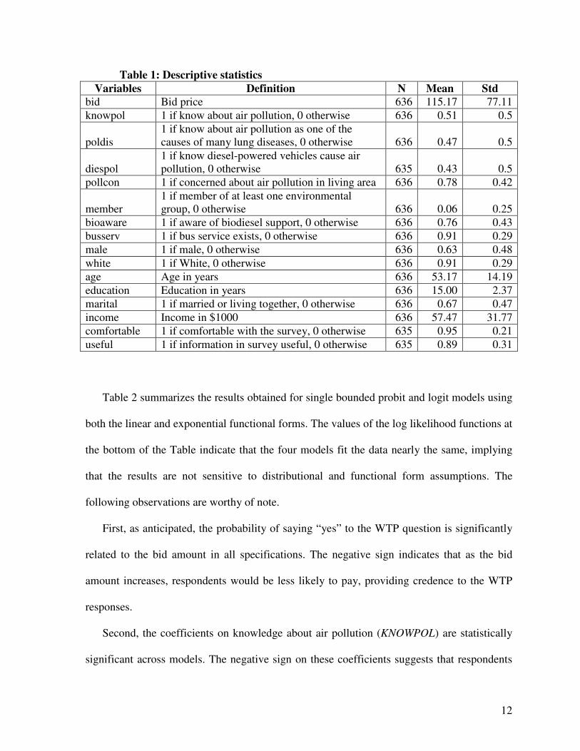
636 were usable. Descriptive statistics are shown in Table 1. For instance, it can be seen that

78% of the respondents were concerned about air pollution in their areas; about 76% stated

that they were aware of the fact that lawmakers, agricultural groups, and clean air advocates

had agreed on the use of biodiesel as a way to reduce emissions from diesel-powered

vehicles. Most respondents were White, male represented 63%, and 67% were married or

lived with a partner. For more details on the survey results, refer to Jeanty (2006).

0

5

10

15

20

25

30

35

% of respondents

Definitely No Probably No Not Sure Probably Yes Definitely Yes

Second bid response choices

No

Yes

12

Table 1: Descriptive statistics Variables Definition N Mean Std

bid Bid price 636 115.17 77.11

knowpol 1 if know about air pollution, 0 otherwise 636 0.51 0.5

poldis 1 if know about air pollution as one of the causes of many lung diseases, 0 otherwise 636 0.47 0.5

diespol 1 if know diesel-powered vehicles cause air pollution, 0 otherwise 635 0.43 0.5

pollcon 1 if concerned about air pollution in living area 636 0.78 0.42

member 1 if member of at least one environmental group, 0 otherwise 636 0.06 0.25

bioaware 1 if aware of biodiesel support, 0 otherwise 636 0.76 0.43

busserv 1 if bus service exists, 0 otherwise 636 0.91 0.29

male 1 if male, 0 otherwise 636 0.63 0.48

white 1 if White, 0 otherwise 636 0.91 0.29

age Age in years 636 53.17 14.19

education Education in years 636 15.00 2.37

marital 1 if married or living together, 0 otherwise 636 0.67 0.47

income Income in $1000 636 57.47 31.77

comfortable 1 if comfortable with the survey, 0 otherwise 635 0.95 0.21

useful 1 if information in survey useful, 0 otherwise 635 0.89 0.31

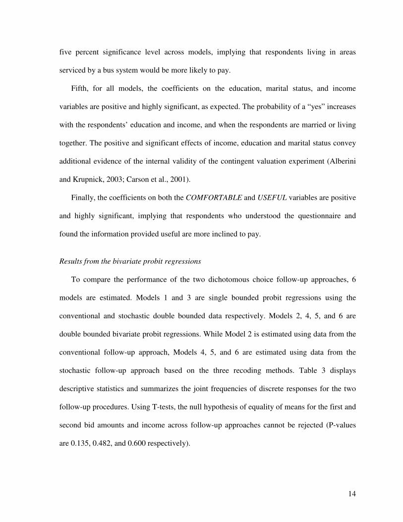
Table 2 summarizes the results obtained for single bounded probit and logit models using

both the linear and exponential functional forms. The values of the log likelihood functions at

the bottom of the Table indicate that the four models fit the data nearly the same, implying

that the results are not sensitive to distributional and functional form assumptions. The

following observations are worthy of note.

First, as anticipated, the probability of saying “yes” to the WTP question is significantly

related to the bid amount in all specifications. The negative sign indicates that as the bid

amount increases, respondents would be less likely to pay, providing credence to the WTP

responses.

Second, the coefficients on knowledge about air pollution (KNOWPOL) are statistically

significant across models. The negative sign on these coefficients suggests that respondents

13

who know more about air pollution would be less inclined to pay. This counter-intuitive

result is similar to findings by Carlsson and Johansson-Stenman (2000), and

Vassanadumrongdee and Matsuoka (2005). One would expect that air pollution

knowledgeable respondents would be more disposed to pay than those learning of the

problems for the first time. A possible explanation is that these respondents may view the

problems less saliently as opposed to less informed respondents. Alternatively, the

coefficients on the variable POLDIS are significant at the five percent significance level and

have a positive sign in all models. This variable takes on the value of one if respondents state

that they know about air pollution as one of the leading causes of many lung diseases, and

zero otherwise. This result suggests that those who hold this view tend to express higher

willingness to pay.

Third, in all specifications, the coefficients on POLLCON are statically related to the

likelihood of saying “yes” to the first WTP question. The positive sign implies that

respondents expressing concern about air pollution in their areas would be more likely to

contribute to the project. This result is consistent with the view of Vassanadumrongdee and

Matsuoka (2005) that respondents who ranked air pollution as their greatest concern would

be more likely to pay.

Fourth, the respondents were asked to provide an approximation about how far they live

from a major highway, a bus stop or route, and a railroad. About half of the respondents

provided incomplete responses to these questions. Some respondents stated that they do not

know or wrote responses with a question mark. Others indicated that bus services are not

available in their cities. We use a dummy variable (BUSSERV) in lieu of inaccurately

measured distance variables. The coefficients have a positive sign and are significant at the

14

five percent significance level across models, implying that respondents living in areas

serviced by a bus system would be more likely to pay.

Fifth, for all models, the coefficients on the education, marital status, and income

variables are positive and highly significant, as expected. The probability of a “yes” increases

with the respondents’ education and income, and when the respondents are married or living

together. The positive and significant effects of income, education and marital status convey

additional evidence of the internal validity of the contingent valuation experiment (Alberini

and Krupnick, 2003; Carson et al., 2001).

Finally, the coefficients on both the COMFORTABLE and USEFUL variables are positive

and highly significant, implying that respondents who understood the questionnaire and

found the information provided useful are more inclined to pay.

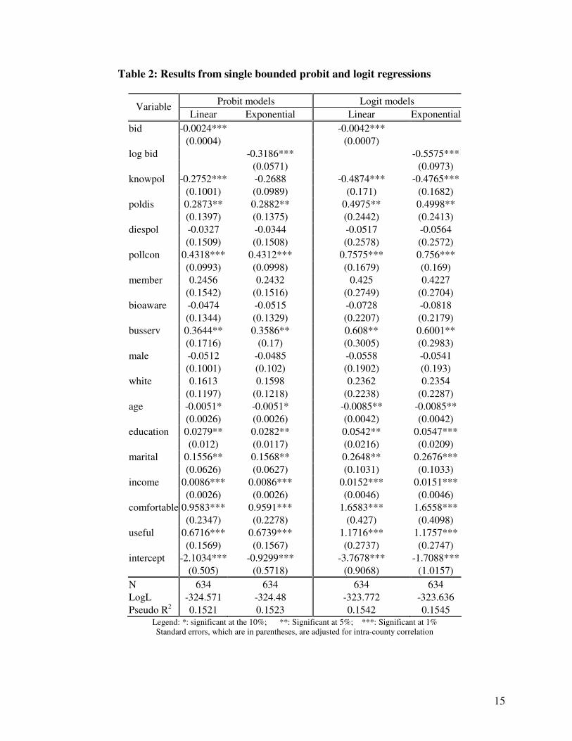
Results from the bivariate probit regressions

To compare the performance of the two dichotomous choice follow-up approaches, 6

models are estimated. Models 1 and 3 are single bounded probit regressions using the

conventional and stochastic double bounded data respectively. Models 2, 4, 5, and 6 are

double bounded bivariate probit regressions. While Model 2 is estimated using data from the

conventional follow-up approach, Models 4, 5, and 6 are estimated using data from the

stochastic follow-up approach based on the three recoding methods. Table 3 displays

descriptive statistics and summarizes the joint frequencies of discrete responses for the two

follow-up procedures. Using T-tests, the null hypothesis of equality of means for the first and

second bid amounts and income across follow-up approaches cannot be rejected (P-values

are 0.135, 0.482, and 0.600 respectively).

15

Table 2: Results from single bounded probit and logit regressions

Probit models Logit models Variable

Linear Exponential Linear Exponential

bid -0.0024*** -0.0042***

(0.0004) (0.0007)

log bid -0.3186*** -0.5575***

(0.0571) (0.0973)

knowpol -0.2752*** -0.2688 -0.4874*** -0.4765***

(0.1001) (0.0989) (0.171) (0.1682)

poldis 0.2873** 0.2882** 0.4975** 0.4998**

(0.1397) (0.1375) (0.2442) (0.2413)

diespol -0.0327 -0.0344 -0.0517 -0.0564

(0.1509) (0.1508) (0.2578) (0.2572)

pollcon 0.4318*** 0.4312*** 0.7575*** 0.756***

(0.0993) (0.0998) (0.1679) (0.169)

member 0.2456 0.2432 0.425 0.4227

(0.1542) (0.1516) (0.2749) (0.2704)

bioaware -0.0474 -0.0515 -0.0728 -0.0818

(0.1344) (0.1329) (0.2207) (0.2179)

busserv 0.3644** 0.3586** 0.608** 0.6001**

(0.1716) (0.17) (0.3005) (0.2983)

male -0.0512 -0.0485 -0.0558 -0.0541

(0.1001) (0.102) (0.1902) (0.193)

white 0.1613 0.1598 0.2362 0.2354

(0.1197) (0.1218) (0.2238) (0.2287)

age -0.0051* -0.0051* -0.0085** -0.0085**

(0.0026) (0.0026) (0.0042) (0.0042)

education 0.0279** 0.0282** 0.0542** 0.0547***

(0.012) (0.0117) (0.0216) (0.0209)

marital 0.1556** 0.1568** 0.2648** 0.2676***

(0.0626) (0.0627) (0.1031) (0.1033)

income 0.0086*** 0.0086*** 0.0152*** 0.0151***

(0.0026) (0.0026) (0.0046) (0.0046)

comfortable 0.9583*** 0.9591*** 1.6583*** 1.6558***

(0.2347) (0.2278) (0.427) (0.4098)

useful 0.6716*** 0.6739*** 1.1716*** 1.1757***

(0.1569) (0.1567) (0.2737) (0.2747)

intercept -2.1034*** -0.9299*** -3.7678*** -1.7088***

(0.505) (0.5718) (0.9068) (1.0157)

N 634 634 634 634

LogL -324.571 -324.48 -323.772 -323.636

Pseudo R2 0.1521 0.1523 0.1542 0.1545 Legend: *: significant at the 10%; **: Significant at 5%; ***: Significant at 1% Standard errors, which are in parentheses, are adjusted for intra-county correlation

16

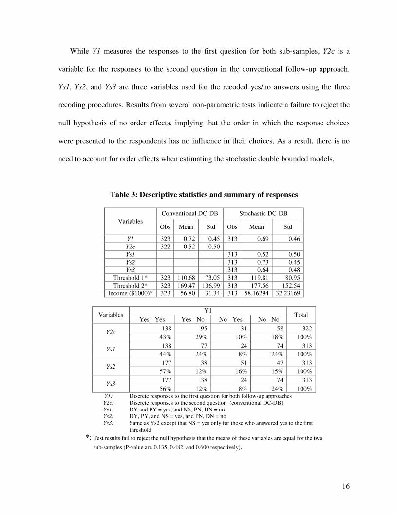
While Y1 measures the responses to the first question for both sub-samples, Y2c is a

variable for the responses to the second question in the conventional follow-up approach.

Ys1, Ys2, and Ys3 are three variables used for the recoded yes/no answers using the three

recoding procedures. Results from several non-parametric tests indicate a failure to reject the

null hypothesis of no order effects, implying that the order in which the response choices

were presented to the respondents has no influence in their choices. As a result, there is no

need to account for order effects when estimating the stochastic double bounded models.

Table 3: Descriptive statistics and summary of responses

Conventional DC-DB Stochastic DC-DB

Variables Obs Mean Std Obs Mean Std

Y1 323 0.72 0.45 313 0.69 0.46

Y2c 322 0.52 0.50

Ys1 313 0.52 0.50

Ys2 313 0.73 0.45

Ys3 313 0.64 0.48

Threshold 1* 323 110.68 73.05 313 119.81 80.95

Threshold 2* 323 169.47 136.99 313 177.56 152.54

Income ($1000)* 323 56.80 31.34 313 58.16294 32.23169

Y1

Variables Yes - Yes Yes - No No - Yes No - No

Total

138 95 31 58 322 Y2c

43% 29% 10% 18% 100%

138 77 24 74 313 Ys1

44% 24% 8% 24% 100%

177 38 51 47 313 Ys2

57% 12% 16% 15% 100%

177 38 24 74 313 Ys3

56% 12% 8% 24% 100% Y1: Discrete responses to the first question for both follow-up approaches Y2c: Discrete responses to the second question (conventional DC-DB) Ys1: DY and PY = yes, and NS, PN, DN = no Ys2: DY, PY, and NS = yes, and PN, DN = no Ys3: Same as Ys2 except that NS = yes only for those who answered yes to the first

threshold

*: Test results fail to reject the null hypothesis that the means of these variables are equal for the two

sub-samples (P-value are 0.135, 0.482, and 0.600 respectively).

17

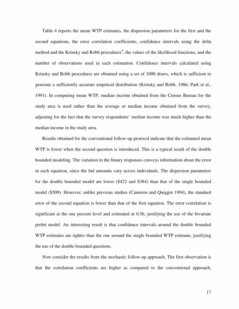
Table 4 reports the mean WTP estimates, the dispersion parameters for the first and the

second equations, the error correlation coefficients, confidence intervals using the delta

method and the Krinsky and Robb procedures4, the values of the likelihood functions, and the

number of observations used in each estimation. Confidence intervals calculated using

Krinsky and Robb procedures are obtained using a set of 1000 draws, which is sufficient to

generate a sufficiently accurate empirical distribution (Krinsky and Robb, 1986; Park et al.,

1991). In computing mean WTP, median income obtained from the Census Bureau for the

study area is used rather than the average or median income obtained from the survey,

adjusting for the fact that the survey respondents’ median income was much higher than the

median income in the study area.

Results obtained for the conventional follow-up protocol indicate that the estimated mean

WTP is lower when the second question is introduced. This is a typical result of the double

bounded modeling. The variation in the binary responses conveys information about the error

in each equation, since the bid amounts vary across individuals. The dispersion parameters

for the double bounded model are lower ($422 and $384) than that of the single bounded

model ($509). However, unlike previous studies (Cameron and Quiggin 1994), the standard

error of the second equation is lower than that of the first equation. The error correlation is

significant at the one percent level and estimated at 0.56, justifying the use of the bivariate

probit model. An interesting result is that confidence intervals around the double bounded

WTP estimates are tighter than the one around the single bounded WTP estimate, justifying

the use of the double bounded questions.

Now consider the results from the stochastic follow-up approach. The first observation is

that the correlation coefficients are higher as compared to the conventional approach,

18

indicating a potential for efficiency gain even if the estimated mean WTP estimates for the

two questions are different. Second, the gap between the single bounded and the double

bounded mean WTP estimates is slightly lower as compared to the results in the conventional

follow-up approach and in previous studies. Now as in previous studies, the dispersion

parameters in the second question are higher than in the first question. Responses to the

second WTP question seem to contain more statistical noise than responses to the first

question. Also, responses to the second question in the stochastic follow-up are noisier than

those in the conventional follow-up. When “not sure” is recoded as “yes”, the second

question yields higher mean WTP estimates than the first question.

It can be seen that confidence intervals around the stochastic double bounded WTP

estimates (models 3, 4, 5, and 6) are tighter those around the conventional double bounded

WTP estimates (models 1 and 2). However, among the stochastic double bounded models

only model 4 yields a more efficient WTP estimate than the single bounded model (model 3),

which appears slightly more efficient than model 6. Since the correlation coefficients are

considerably higher than 0.5, efficiency gain can be obtained by constraining the means and

the dispersion parameters to be the same across equations or questions. However, the data

need to respond in kind.

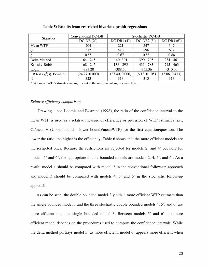
Results from restricted bivariate probit regressions

Models 2, 4, 5, and 6 were re-estimated, constraining the means and the dispersion

parameters to be identical for both questions5. Table 5 reports the results from the restricted

bivariate probit regressions (models 2’, 4’, 5’ and 6’). Again, compared to the single bounded

model, the mean WTP estimate decreases more sharply in the conventional follow-up than in

the stochastic follow-up models when the second question is taken into account. For models

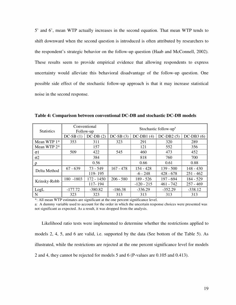
19

5’ and 6’, mean WTP actually increases in the second equation. That mean WTP tends to

shift downward when the second question is introduced is often attributed by researchers to

the respondent’s strategic behavior on the follow-up question (Haab and McConnell, 2002).

These results seem to provide empirical evidence that allowing respondents to express

uncertainty would alleviate this behavioral disadvantage of the follow-up question. One

possible side effect of the stochastic follow-up approach is that it may increase statistical

noise in the second response.

Table 4: Comparison between conventional DC-DB and stochastic DC-DB models

Conventional Follow-up

Stochastic follow-upa Statistics

DC-SB (1) DC-DB (2) DC-SB (3) DC-DB1 (4) DC-DB2 (5) DC-DB3 (6)

Mean WTP 1* 353 311 323 291 320 289

Mean WTP 2* 157 121 552 356

σ1 509 422 545 460 473 452

σ2 384 818 760 700

ρ 0.56 0.66 0.61 0.88

67 - 639 73 - 549 167 - 478 154 - 428 139 - 500 148 - 430 Delta Method

119- 195 -6 - 248 428 - 678 251 - 462

180 -1803 172 - 1450 206 - 580 189 - 526 197 - 694 184 - 529 Krinsky-Robb

117- 194 -120 - 215 461 - 742 257 - 469

LogL -177.72 -380.82 -186.38 -336.29 -352.29 -338.12 N 323 323 313 313 313 313

*: All mean WTP estimates are significant at the one percent significance level. a: A dummy variable used to account for the order in which the uncertain response choices were presented was not significant as expected. As a result, it was dropped from the analysis.

Likelihood ratio tests were implemented to determine whether the restrictions applied to

models 2, 4, 5, and 6 are valid, i.e. supported by the data (See bottom of the Table 5). As

illustrated, while the restrictions are rejected at the one percent significance level for models

2 and 4, they cannot be rejected for models 5 and 6 (P-values are 0.105 and 0.413).

20

Table 5: Results from restricted bivariate probit regressions

Conventional DC-DB Stochastic DC-DB Statistics

DC-DB (2’) DC-DB1 (4’) DC-DB2 (5’) DC-DB3 (6’)

Mean WTP* 204 221 547 347

σ 312 520 896 637

ρ 0.55 0.67 0.58 0.88

Delta Method 164 - 245 140 -301 390 - 705 234 - 461

Krinsky-Robb 168 - 245 138 - 295 431 - 783 245 - 463

LogL -393.20 -388.50 -355.36 -340.00

LR test (χ2(3), P-value) (24.77, 0.000) (23.40, 0.000) (6.13, 0.105) (2.86, 0.413)

N 323 313 313 313

*: All mean WTP estimates are significant at the one percent significance level.

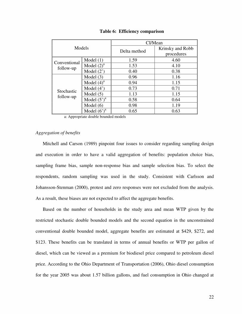
Relative efficiency comparison

Drawing upon Loomis and Ekstrand (1998), the ratio of the confidence interval to the

mean WTP is used as a relative measure of efficiency or precision of WTP estimates (i.e.,

CI/mean = (Upper bound – lower bound)/meanWTP) for the first equation/question. The

lower the ratio, the higher is the efficiency. Table 6 shows that the more efficient models are

the restricted ones. Because the restrictions are rejected for models 2’ and 4’ but hold for

models 5’ and 6’, the appropriate double bounded models are models 2, 4, 5’, and 6’. As a

result, model 1 should be compared with model 2 in the conventional follow-up approach

and model 3 should be compared with models 4, 5’ and 6’ in the stochastic follow-up

approach.

As can be seen, the double bounded model 2 yields a more efficient WTP estimate than

the single bounded model 1 and the three stochastic double bounded models 4, 5’, and 6’ are

more efficient than the single bounded model 3. Between models 5’ and 6’, the more

efficient model depends on the procedures used to compute the confidence intervals. While

the delta method portrays model 5’ as more efficient, model 6’ appears more efficient when

21

considering the Krinsky and Robb procedures. Because the WTP measure yielded by model

5’ is noisier, one may prefer model 6’. In addition, since WTP measures are non-linear

combinations of the parameter estimates, they are less likely to be normally distributed and

thus non-symmetric around the means. Percentile non-symmetric confidence intervals given

by the Krinsky and Robb (KR) method would be more appropriate. Note the larger efficiency

gain provided by model 2’ as compared with all other estimated models. However, this

efficiency gain comes at the cost of biasness since the restrictions are rejected at the one

percent significant level.

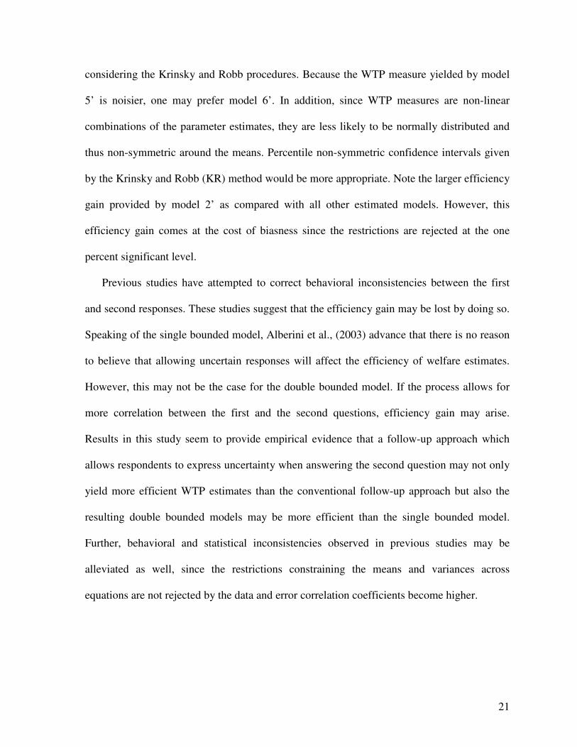
Previous studies have attempted to correct behavioral inconsistencies between the first

and second responses. These studies suggest that the efficiency gain may be lost by doing so.

Speaking of the single bounded model, Alberini et al., (2003) advance that there is no reason

to believe that allowing uncertain responses will affect the efficiency of welfare estimates.

However, this may not be the case for the double bounded model. If the process allows for

more correlation between the first and the second questions, efficiency gain may arise.

Results in this study seem to provide empirical evidence that a follow-up approach which

allows respondents to express uncertainty when answering the second question may not only

yield more efficient WTP estimates than the conventional follow-up approach but also the

resulting double bounded models may be more efficient than the single bounded model.

Further, behavioral and statistical inconsistencies observed in previous studies may be

alleviated as well, since the restrictions constraining the means and variances across

equations are not rejected by the data and error correlation coefficients become higher.

22

Table 6: Efficiency comparison

CI/Mean Models

Delta method Krinsky and Robb

procedures

Model (1) 1.59 4.60 Model (2)a 1.53 4.10

Conventional follow-up

Model (2’) 0.40 0.38

Model (3) 0.96 1.16

Model (4)a 0.94 1.15

Model (4’) 0.73 0.71

Model (5) 1.13 1.15

Model (5’)a 0.58 0.64

Model (6) 0.98 1.19

Stochastic follow-up

Model (6’)a 0.65 0.63 a: Appropriate double bounded models

Aggregation of benefits

Mitchell and Carson (1989) pinpoint four issues to consider regarding sampling design

and execution in order to have a valid aggregation of benefits: population choice bias,

sampling frame bias, sample non-response bias and sample selection bias. To select the

respondents, random sampling was used in the study. Consistent with Carlsson and

Johansson-Stenman (2000), protest and zero responses were not excluded from the analysis.

As a result, these biases are not expected to affect the aggregate benefits.

Based on the number of households in the study area and mean WTP given by the

restricted stochastic double bounded models and the second equation in the unconstrained

conventional double bounded model, aggregate benefits are estimated at $429, $272, and

$123. These benefits can be translated in terms of annual benefits or WTP per gallon of

diesel, which can be viewed as a premium for biodiesel price compared to petroleum diesel

price. According to the Ohio Department of Transportation (2006), Ohio diesel consumption

for the year 2005 was about 1.57 billion gallons, and fuel consumption in Ohio changed at

23

the same rate as the Ohio population from 1970 to 2005. Relying on population data, diesel

consumption in the study area is estimated at 257.84 million gallons for 2005, yielding a

premium for biodiesel price estimated at nine, 31, and 20 cents for the three models

respectively.

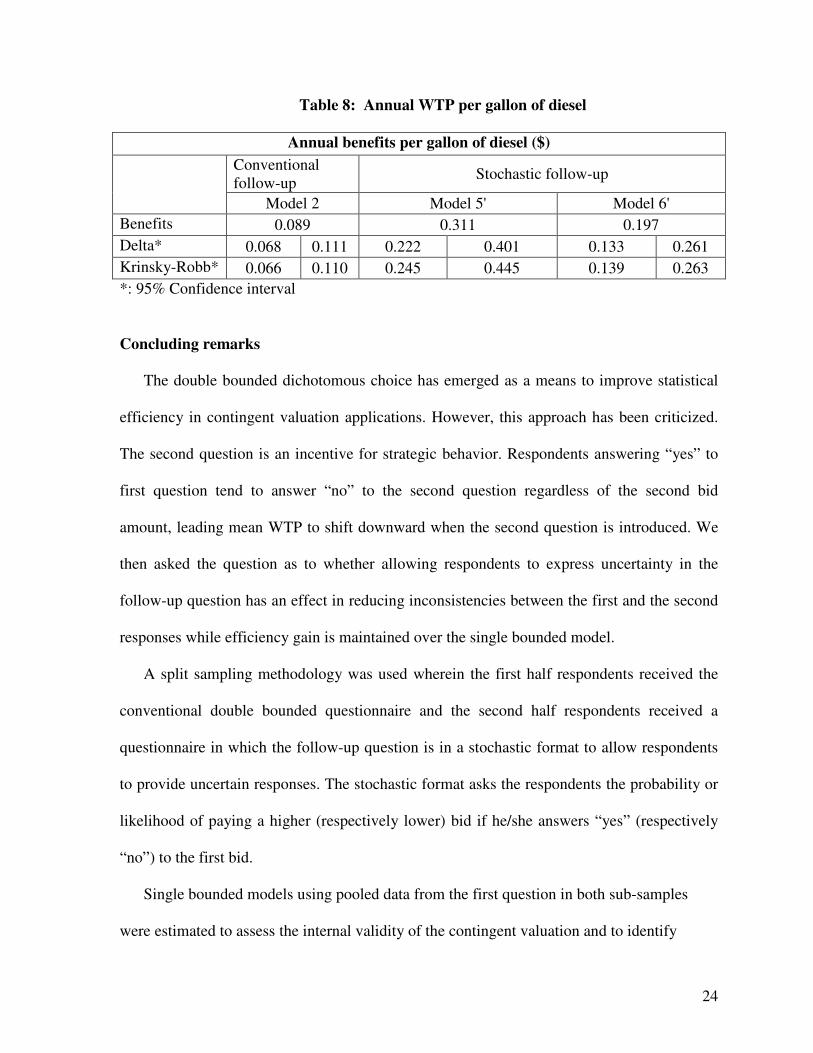
Since model 6’ is the most efficient, the appropriate premium lies in the confidence

interval of 14 to 26 cents, as shown in Table 8. These results suggest that if a policy aiming

at promoting biodiesel production and use entails charging a premium within the above

range, consumers would be willing to pay it because of the environmental benefits they will

reap. Put differently, a price differential between pure diesel and blended or pure biodiesel

would be justified from the perspective of the consumers. It is worth noting that the estimated

premium range is consistent with the price differential range, 15 to 30 cents, observed in

recent years.

Table 7: Aggregate benefits and their confidence intervals

Conventional follow-up

Stochastic follow-up

Model 2 ($106) Model 5’ ($106) Model 6’($106)

Benefits 123.05 428.70 271.95

Delta 93.26 - 152.83 305.66 - 552.53 183.39 - 360.52

Krinsky-Robb 91.70 - 152.04 337.79 - 613.66 192.01 - 362.87 N.B.: For annual benefits, these numbers need to be divided by 5.

24

Table 8: Annual WTP per gallon of diesel

Annual benefits per gallon of diesel ($)

Conventional follow-up

Stochastic follow-up

Model 2 Model 5' Model 6'

Benefits 0.089 0.311 0.197

Delta* 0.068 0.111 0.222 0.401 0.133 0.261

Krinsky-Robb* 0.066 0.110 0.245 0.445 0.139 0.263

*: 95% Confidence interval

Concluding remarks

The double bounded dichotomous choice has emerged as a means to improve statistical

efficiency in contingent valuation applications. However, this approach has been criticized.

The second question is an incentive for strategic behavior. Respondents answering “yes” to

first question tend to answer “no” to the second question regardless of the second bid

amount, leading mean WTP to shift downward when the second question is introduced. We

then asked the question as to whether allowing respondents to express uncertainty in the

follow-up question has an effect in reducing inconsistencies between the first and the second

responses while efficiency gain is maintained over the single bounded model.

A split sampling methodology was used wherein the first half respondents received the

conventional double bounded questionnaire and the second half respondents received a

questionnaire in which the follow-up question is in a stochastic format to allow respondents

to provide uncertain responses. The stochastic format asks the respondents the probability or

likelihood of paying a higher (respectively lower) bid if he/she answers “yes” (respectively

“no”) to the first bid.

Single bounded models using pooled data from the first question in both sub-samples

were estimated to assess the internal validity of the contingent valuation and to identify

25

determinants of WTP. The results confirm the validity of the contingent valuation and are

consistent with findings in most contingent valuation studies.

Comparing the two follow-up approaches results indicate that the stochastic format yields

more efficient WTP estimates than the regular or conventional follow-up approach by

increasing the correlation between the first and the second responses. Since the error

correlation coefficients are considerably above 0.5, efficiency gain can be obtained by

constraining both means and variances to be the same across questions. Four restricted

models were then estimated: one conventional double bounded model and three stochastic

double bounded models. Whereas the restrictions were rejected for the conventional double

bounded model, they hold for two of the stochastic double bounded models. Since the

restricted stochastic double bounded models are valid and more efficient than the single

bounded model, allowing respondents to express uncertainty in the follow-up question seems

to reduce the strategic behavior while maintaining efficiency gain. Statistical inconsistencies

seem to be alleviated also since the error correlation coefficients increase in the stochastic

double bounded models.

The restricted conventional double bounded model is more efficient than the restricted

stochastic double bounded models, but the data did not support the restrictions. Thus, the

efficiency gain comes at the cost of biasness. Since less noisy, the WTP estimate for the

second equation in the unrestricted version of the conventional double bounded model is

used to estimate aggregate benefits at $123 million. Aggregate benefits using the valid

restricted stochastic double bounded models are estimated at $429 million and $272 million

for a five-year period. Energy policy implications of these results are that that the public

would be willing to make money contributions to protect the environment. If the cost of

26

producing and using more biodiesel entails charging a premium, consumers would be willing

to pay it, due to the resulting environmental benefits.

Our hope is that this study will be followed by other applications of the dichotomous

choice format with a stochastic follow-up question. Future research may try implementing a

scope test. The test can be done using both the regular and the stochastic follow-up formats

to determine whether both follow-up versions pass the test. In addition, the recoding

methods used to convert responses from uncertain to certain can be an issue. Results may

vary depending on how uncertain response choices are recoded. Here, we draw upon

previous studies and the pattern of the data to choose the recoding methods. The results in

this study indicate that the recoding procedure relying on the pattern of the data yields the

most efficient and appropriate model. To avoid the issue of recoding, future research using

the stochastic follow-up can attempt to parameterize the likelihood function in a way to

incorporate the uncertain response options directly. One condition that needs to be satisfied is

that respondents must switch from “definitely yes” to more uncertain response categories

(“probably yes”, “not sure” and “probably no”) and to “definitely no” as the magnitude of the

bid increases. In this study, such a behavior was not observed. When such a behavior is

observed then thresholds that further bound WTP can be estimated.

References

Alberini, A. “Optimal Designs for Discrete Choice Contingent Valuation Surveys: Single-

bound, Double-bound, and Bivariate Models.” Journal Environmental Economics and

Management 28 (1995): 287–306.

Alberini, A., and A. Krupnick. “Valuing the Health Effects of Pollution.” In Thomas

Tietenberg and Henk Folmer (eds.). The International Yearbook of Environmental and

Resource Economics 2002/2003. Northampton, MA: Edward Elgar, 2003.

Alberini, A., K. Boyle, and M. Welsh. “Analysis of Contingent Valuation Data with Multiple

Bids and Response Options Allowing Respondents to Express Uncertainty.” Journal of

Environmental Economics and Management 45(2003): 40-62.

Arrow, K.R., P.R. Solow, E.E. Portney, R. Leamer, R. Radner, and H. Schuman. “Report of

the NOAA Panel on Contingent Valuation.” Federal Register 58(1993): 4601-4614.

Banzhaf, S., B. Dallas, D. Evans, and A. Krupnick. “Valuation of Natural Resource

improvements in the Adronacks.” Resource for the Future, Washington DC, 2004.

Bateman, I. J., B.H. Day, D. P. Dupont, and Stavros Georgiou. Incentive Compatibility and

Procedural Invariance Testing of the One-And-One-Half-Bound Dichotomous Choice

Elicitation Method: Distinguishing Strategic Behaviour from the Anchoring Heuristic.

(May 2006) unpublished.

http://academy.atlanticwebfitters.ca/Portals/0/CREEpapers/Dupont_Diane.pdf

Bateman, I. J., I. H. Langford, A. P. Jones, and G. N. Kerr. “Bound and Path Effects in

Double Bounded and Triple Bounded Dichotomous Choice Contingent Valuation.”

Resource and Energy Economics 23(2001): 181–213.

Callia, P., and E. Strazzera. “Bias and Efficiency of Single vs. Double Bound Models for

Contingent Valuation Studies: a Monte Carlo Analysis.” Applied Economics 32(2000):

1329-1336.

Cameron, T.A., and J. Quiggin. “Estimation Using Contingent Valuation Data from a

Dichotomous Choice with Follow-up Questionnaire.” Journal of Environmental

Economics and Management 27(1994): 218-34.

Carlsson, F., and O. Johansson-Stenman. “Willingness to Pay for Improved Air Quality in

Sweden.” Applied Economics 32 (2000): 661-69.

Carson, R.T. “Contingent Valuation: A User’s Guide.” Environmental Science and

Technology 34 (2000): 1413-1418.

Carson, R.T., N.E. Flores, and N.F. Meade. “Contingent Valuation: Controversies and

Evidence.” Environmental and Resources Economics 19(2001): 173-210.

Carson, R.T., W.M. Hanemann, R.J. Kopp, J.A. Krosnick, R.C. Mitchell, S. Presser, P.A.

Ruud, and V.K. Smith. “Referendum Design and Contingent Valuation Method: The

N.O.A.A. Panel’s No Vote Recommendation.” Review of Economics and Statistics

80(1998): 1998.

Cooper, J.,W.M. Hanemann, and G. Signorelli. “One and One-half Bids Dichotomous

Choice Contingent Valuation.” The Review of Economics and Statistics 84(2002): 742-

750.

Dillman, D.A. Mail and Internet Surveys: The Tailored Design Method. 2nd ed. New York,

NY: John Wiley & Sons, 2000.

Haab, T.C. “Analyzing Multiple Question Contingent Valuation Surveys: A Reconsideration

of the Bivariate probit.” Department of Economics, East Carolina University, Greenville,

NC 27858, 1997.

Haab, T.C., and K.E. McConnell. Valuing Environmental Natural Resources: The

Econometrics of Non-Market Valuation. Northampton, MA: Edward Elgar Publishing,

2002.

Hanemann, W.M., J. Loomis, and B.J. Kanninen. “Statistical Efficiency of Double-bounded

Dichotomous Choice Contingent Valuation.” American Journal of Agricultural

Economics 73 (1991): 1255-263.

Harrison, G.W., and B. Kriström. “On the Interpretation of Responses in Contingent

Surveys”, in P-O. Johansson, B. Kriström and K-G. Mäler, ed., Current Issues in

Environment Economics, Manchester University Press (1995): 35-57.

Huang, J., and V.K. Smith. “Monte Carlo Benchmarks for Discrete Valuation Methods.”

Land Economics 74(1998): 186-202.

Jeanty, P.W. Two Essays on Environmental and Food Security. Unpublished Dissertation.

The Ohio State University, Columbus, OH, 2006.

Krinsky, I., and A.L. Robb. “On Approximating the Statistical Properties of Elasticities.”

Review of Economic and Statistics 68(1986): 715-719.

Li, C., and L. Mattsson. “Discrete Choice under Preference Uncertainty: An Improved

Structural Model for Contingent Valuation.” Journal of Environmental Economics and

Management 28 (1995): 256 – 69.

Loomis, J., and E. Ekstrand. “Alternative Approach for Incorporating Uncertainty When

Estimating Willingness to Pay: The Case of the Mexican Spotted Owl.” Ecological

Economics 27(1998): 29-41.

Loureiro, M., A. Gracia, and R.M. Nayga. “Do Consumers Value Nutritional Labels?”

European Journal of Agricultural Economics 33(2006): 249-268.

McLeod, D.M., and O. Bergland. “Willingness-to-Pay Estimates Using the Double-Bounded

Dichotomous-Choice Contingent Valuation Format: A Test for Validity and Precision in a

Bayesian Framework.” Land Economics 75 (1999): 115-125.

Mitchell, R. and R. Carson. “Using Surveys to Value Public Goods.” Resources for the

Future, Washington D.C., 1989.

Moran, D., and A.S. Moraes. “Contingent Valuation in Brazil: An Estimation of Pollution

Damage in the Pantanal.” In Natural Resources Valuation and Policy in Brazil: Methods

and Cases, eds. Peter H May and Mary C. Paul, Columbia University Press, New York,

1999.

Ohio Department of Transportation. Financial and Statistical Report, Columbus, OH, 2006

Park, T., J.B. Loomis, and M. Creel. “Confidence Interval for Evaluating Benefits Estimates

from Dichotomous Choice Contingent Valuation Studies.” Land Economics 67(1991): 64-

73

Vassanadumrongdee, S., and S. Matsuoka. “Risk Perceptions and Value of a Statistical Life

for Air Pollution and Traffic Accident: Evidence from Bangkok, Thailand.” The Journal

of Risk and Uncertainty 30(2005): 261-287.

Welsh, M.P., and G.L. Poe. “Elicitation Effects in Contingent Valuation: Comparison to a

Multiple Bounded Discrete Choice Approach.” Journal of Environmental Economics and

Management 36 (1998): 170-185.

Yoo, S., and K. Chae. “Measuring the Economic Benefits of the Ozone Pollution Control

Policy in Seoul: Results of a Contingent Valuation Survey.” Urban Studies 38(2001): 49-

60.

Appendix: Valuation Questions with both Conventional and Stochastic Follow-up Formats

Valuation questions with conventional follow-up format

Please answer the following questions:

14. If fundings were available, would you favor

a cleaner environment? Please circle one of

the following:

1. Yes

2. No

When answering the following questions, please

think of your income and what producing and

using more biodiesel in Ohio are worth to your

household.

15. Suppose this project could be completed in 5

years and is estimated to cost your household

a lump sum payment of $X to the trust fund.

Suppose further that payment arrangement

allows you to spread out your payment over

one year. If an election were held today,

would you vote for the project?

1. Yes

2. No

If you said Yes, please continue to question 16

If you said No, please Skip to question 17

16. Suppose instead the project would cost

your household a lump sum payment of

$Y (>X), would you still vote for it?

Please circle one of the following:

1. Yes

2. No

Now skip to question 18

17. Suppose instead the project would cost

your household a lump sum payment of

$Z (<X), would you now vote for it?

Please circle one of the following:

1. Yes

2. No

(Continue to question 18)

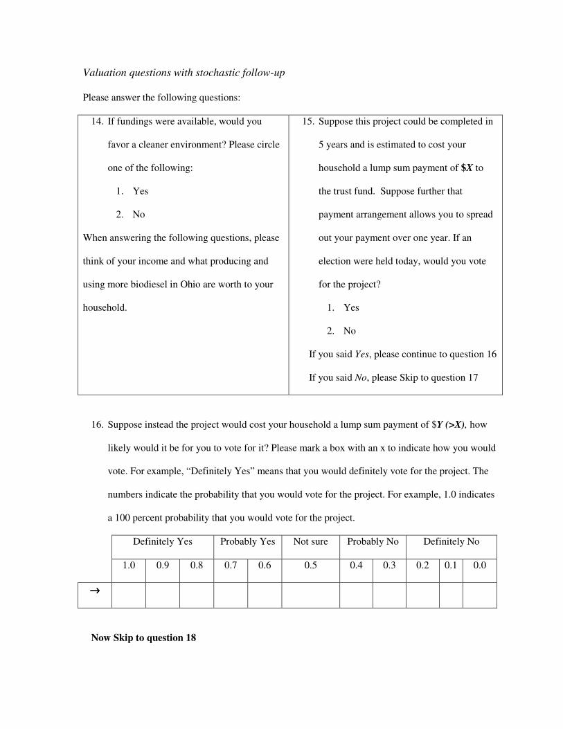
Valuation questions with stochastic follow-up

Please answer the following questions:

14. If fundings were available, would you

favor a cleaner environment? Please circle

one of the following:

1. Yes

2. No

When answering the following questions, please

think of your income and what producing and

using more biodiesel in Ohio are worth to your

household.

15. Suppose this project could be completed in

5 years and is estimated to cost your

household a lump sum payment of $X to

the trust fund. Suppose further that

payment arrangement allows you to spread

out your payment over one year. If an

election were held today, would you vote

for the project?

1. Yes

2. No

If you said Yes, please continue to question 16

If you said No, please Skip to question 17

16. Suppose instead the project would cost your household a lump sum payment of $Y (>X), how

likely would it be for you to vote for it? Please mark a box with an x to indicate how you would

vote. For example, “Definitely Yes” means that you would definitely vote for the project. The

numbers indicate the probability that you would vote for the project. For example, 1.0 indicates

a 100 percent probability that you would vote for the project.

Definitely Yes Probably Yes Not sure Probably No Definitely No

1.0 0.9 0.8 0.7 0.6 0.5 0.4 0.3 0.2 0.1 0.0

→→→→

Now Skip to question 18

17. Suppose instead the project would cost your household a lump sum payment of $Z (<X), how

likely would it be for you to vote for it? Please mark a box with an x to indicate how you would

vote. For example, “Definitely Yes” means that you would definitely vote for the project. The

numbers indicate the probability that you would vote for the project.

Definitely Yes Probably Yes Not sure Probably No Definitely No

1.0 0.9 0.8 0.7 0.6 0.5 0.4 0.3 0.2 0.1 0.0

→→→→

Continue to question 18

Endnotes 1 Constrained models must be used for inferences if the data support the restrictions from a

statistical standpoint.

2 Explanatory variables included are based on previous studies.

3 For the linear model, mean and median WTP are equivalent

4 The bootstrapping method, although not appropriate here, was attempted. It is very

computationally intensive and thus very unattractive in bivariate probit models.

5 While these models are referred to as random effects probit, we did not use random effects

probit routines. The models are estimated by bivariate probit procedures while applying the

restrictions. Interval data models were also estimated; however, the data did not support the

restrictions imposed by the interval data models. Applying restrictions rejected by the data

would entail imposing one’s will on the data.

Acknowledgment: Jeanty and Hitzhusen acknowledge the support of the Ohio Department

of Development Under Agreement Number (please add the number here)