NWS State College Case Examples

Will Tropical Storm Sandy become the Storm of the 21st Century? By

Richard H. Grumm National Weather Service State College, PA 16803

Contributions by Craig Evanego Abstract The interaction with tropical storm Sandy with a strong mid-latitude trough is predicted to produce a potentially historic storm along the East Coast of the United States on 29-30 October 2012. The storm has been compared to the Perfect Storm of October 1991 and Hurricane Hazel. The massive scope and large standardized anomalies associated with forecasts of this storm have garnered significant media attention. The storm was quoted as being a Franken Storm1 and the megastorm. This paper will show how the extra-tropical transition of Sandy compares to previous storms. If Sandy verifies as predicted, the wind and pressure anomalies would far eclipse those associated with Hazel and the perfect storm. The winds associated with the storm of 26 November 1950 will likely be more comparable to this storm. All of the aforementioned storms were significant in their own right. However the anomalies of key fields associated with Sandy would likely produce an historic storm with significant impacts along the East Coast. From a standard anomalies point of view related to low-level wind anomalies and pressure anomalies the storm of 29-30 October 2012 has the potential to eclipse most comparative storms. This implies it could eclipse these storms in terms of impacts on society. Unlike the Perfect Storm, this storm has a high probability of affecting tens of millions of people in the densely populated corridor from Washington DC to the New York Metropolitan area. 1. Overview Forecasts from the National Centers for Environmental Predictions (NCEP) global forecast system (GFS) and global ensemble forecast system (GEFS) began predicting a potentially historic storm along the East Coast. The European Center for Medium Range Forecast (ECMWF) global model (EC) and global ensemble forecast system also began predicting a potentially historic storm. There has been a convergence of forecasts by all the global modeling centers toward a potentially historic storm along the East Coast of the United States. Forecasts of this storm have been compared to previous record events in history. Some of this comparisons or “analogs” are presented in section 3 below. Analogs and comparisons are interesting to the meteorologist and have some intrinsic value conveying information to the public. However, due to a lack of thousands of years of data (van den Dool 1994) they are of limited operational utility.

1 This term became the headlines in the news after about 25 October but is not a term used by NOAA/NWS

NWS State College Case Examples

The concept of using standardized anomalies to gage the intensity of storms was presented by Hart and Grumm (2001). The concept focused on using normalized anomalies with the NCEP/NCAR re-analysis data to rank historic storms. The value of M-TOTAL, averaging the wind, temperature, height, and moisture anomalies, (MTOTAL = (MTEMP + MHEIGHT + MWIND + MMOIST) / 4 ) produced a list of the historic storms over much of eastern North America and the adjacent Atlantic Ocean. The values of MTEMP are integrated over the mandatory levels in the atmosphere. In addition to characterizing storms based on MTOTAL the storms were sorted by month and by variables such as MTemp and Mwind which identified many historic storms. The largest MTOTAL storm was the great Atlantic Low of January 1956 (Ludlum 1956). The superstorm (Kocin et al. 1995) was had the third highest value of MTOTAL. Tropical storm Hazel (Knox 1955), a storm which the forecasts of Sandy have been compared to, was the ninth highest ranked storm on the list. The value of standardized anomalies in the forecast process was introduced by Grumm and Hart (2001). Follow-on studies have shown the value of using standardized anomalies to predict heavy rains and other high impact weather events has been presented by Junker et al 2009; Bodner et al. 2011;Stuart and Grumm 2009;Grumm 2010. Graham and Grumm (2011) demonstrated the value of standardized anomalies in identifying record events over the western United States. This paper will show forecasts of the potential associated with the extratropical transition of tropical storm Sandy with a strong mid-latitude trough. These forecast when use in conjunction with standardized anomalies implies that this storm has the potential to be an historic storm and could be a top-20 event if it verifies as forecast. In addition to forecasts of the storm some historic storms that have been used as comparisons are presented.

2. Data and Methods

Model include forecasts from the NCEP GFS, GEFS and the European Center model. No verification data is available as the storm is still about 3-4 days out in the future. All anomaly displays are as in Hart and Grumm (2001). All model and anomaly data were plotted using GrADS (Doty and Kinter 1995).

The comparison storms prior to 1979 were reconstructed using the NCEP/NCAR reanalysis data which is on a 2.5x2.5 degree grid (Kalnay 1996. More recent cases are displayed using the Climate Forecast System Version I data on a 0.5x0.5 degree grid (Saha et al. 2006;Saha et al. 2010).

3. Great Comparative Storms in history

NWS State College Case Examples

Tropical storm2 Hazel was a high impact storm along the East Coast of the United States during October 1954. The storm achieved hurricane status and produced flooding in the eastern United States. Near the storms peak in the Mid-Atlantic region at 1800 UTC 15 October 1954 the storm produced -4 to -5σ 850 hPa u-wind anomalies (Fig. 1). The storm had a deep mid-latitude trough interaction, a deep cyclone, and a surge of high precipitable water air (PW) which contributed to the heavy rainfall.

The evolution of the PW plume (Fig. 2) shows the surge of tropical moisture up the East Coast and the approaching second surge of moisture with a frontal system. Features which will be shown are evident in the forecasts with Sandy. The 500 hPa pattern shows the mid-latitude trough interaction with Haze (Fig. 3).

The telling feature are the 850 hPa winds, which peaked near -4.5σ below normal (Fig. 4). The heavy rains, strong winds, and flooding occurred in close proximity to the region affected by the PW anomalies and the 850 hPa u-wind anomalies. It will be shown that the forecasts for Sandy indicated u-wind anomalies on the order of -5 to -6σ below normal and had forecasts of 850 hPa wind anomalies on the order of 6σ above normal.

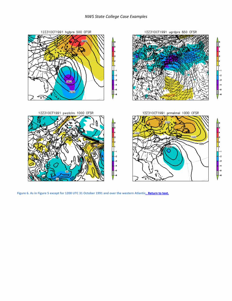
The perfect storm or the Halloween storm of October 1991 is another comparative storm. The storm was a compact storm, relatively small in diameter and it was displaced well out to see (Fig. 5). The cyclone was about -3 σ below normal in the denser CFSR data. The storm produced 6σ wind anomalies at 850 hPa though it was in a narrow band along the coast of New England and the adjacent western Atlantic Ocean. By 1200 UTC 31 October (Fig. 6) though weaker, the storm had retrograded and the strong winds moved farther south along the East Coast, though on -3 to -4σ below normal. Key features included the blocking 500 hPa ridge over the north Atlantic with a massive area of high pressure over eastern North America at the surface, and the cut-off south of the block.

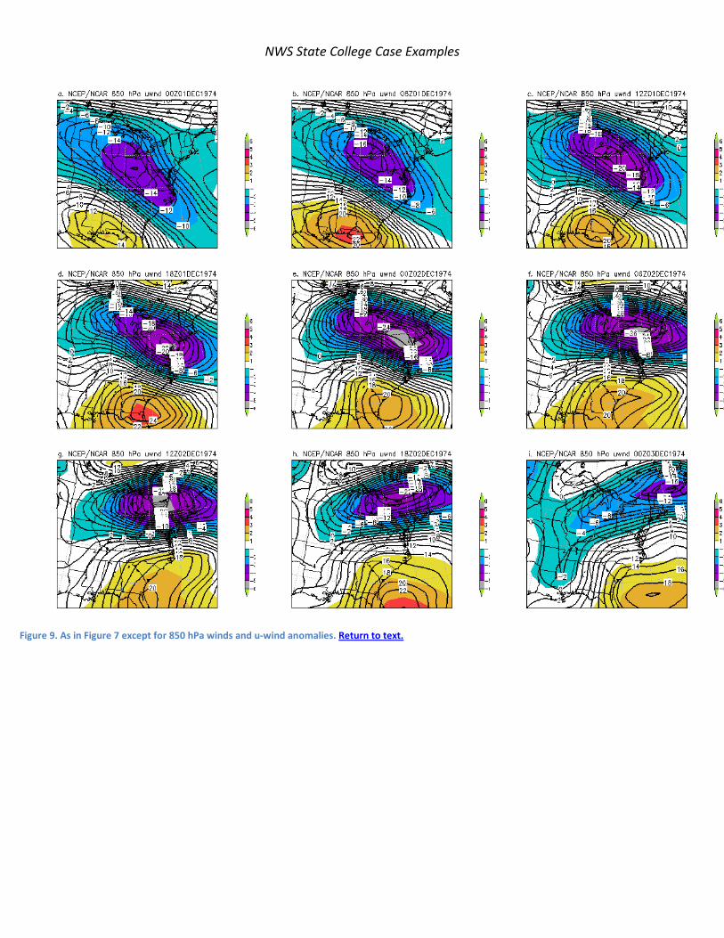
A late season plume of high PW air (Fig. 7) moved up the East Coast and produced a deep cyclone (Fig. 8) which brought wind, rain and heavy snow to the East Coast on 1 December 1974. A banana shaped high was present north of the storm slowing its progress to the north and indicative of blocking, a key theme in many damaging storms. The storm had deep pressure anomalies (Fig. 8) and some of the stronger 850 hPa u-wind anomalies to cover such a broad region (Fig. 9).

One of the last storms, outside of a tropical system, to produce widespread high winds, heavy rains, and winter weather was the storm of 25-26 November 1950. This storm had surge of modestly high PW air into the eastern United States (Fig. 10) and a deep cyclone which retrograded westward (Fig. 11). A contributing factor was the downstream blocking ridge 2 The term tropical storm is used. Many of the storms reached hurricane status such as Sandy and Hazel during their life cycles. However the broader term is used to describe the storm as not to erronesously refer to a storm as hurricane at a time it did not meet the criteria or had undergone extra-tropical transition.

NWS State College Case Examples

allowing the 500 hPa cyclone to cut-off beneath the ridge over eastern Canada (Fig. 12b-g). The storm was one of the few storms to show consistent 6s u-wind anomalies at 850 hPa (Fig. 13d-f). High winds at the surface affected northern New England and many METAR sites in the northeast had record winds recorded with this event. This storm was cited by Changnon and Changnon (1992) listed this storm as one of the significant weather catastrophes in the United States. Table II (Changnon & Changnon 1992) lists Hurricanes Hazel, Hugo, and the 24-27 November 1950 storms among the more damaging storms in US history. The storm produced damaging winds, floods, and heavy snow affecting the southeast and northeastern United States.

Record low pressure is a forecast consideration with this storm too.

Date Low Pressure Location Other Information 3 March 1914 961 New York 7 March 1932 955 Nantucket

21 September 1938 938 Bellport NY Long Island Express 28 March 1984 965 Eastern DelMarva Gyakum and Barker

1988. 14 March 1993 962 White Plains NY Super Storm

Table 1. Record low pressures for cyclone along the East Coast. Courtesy Anton Seimon.

The final case is the March 1984 storm (Gyakum and Barker 1984) which had a low pressure record and had 6s 850 hPa wind anomalies along the East Coast (Fig. 14). This storm too was a notable storm in terms of impacts from the southeast up the East Coast. The region affected by 6s 850 hPa wind anomalies was short-lived and focused along the coastal plain.

4. Forecasts

4.1.1 European Center Forecasts.

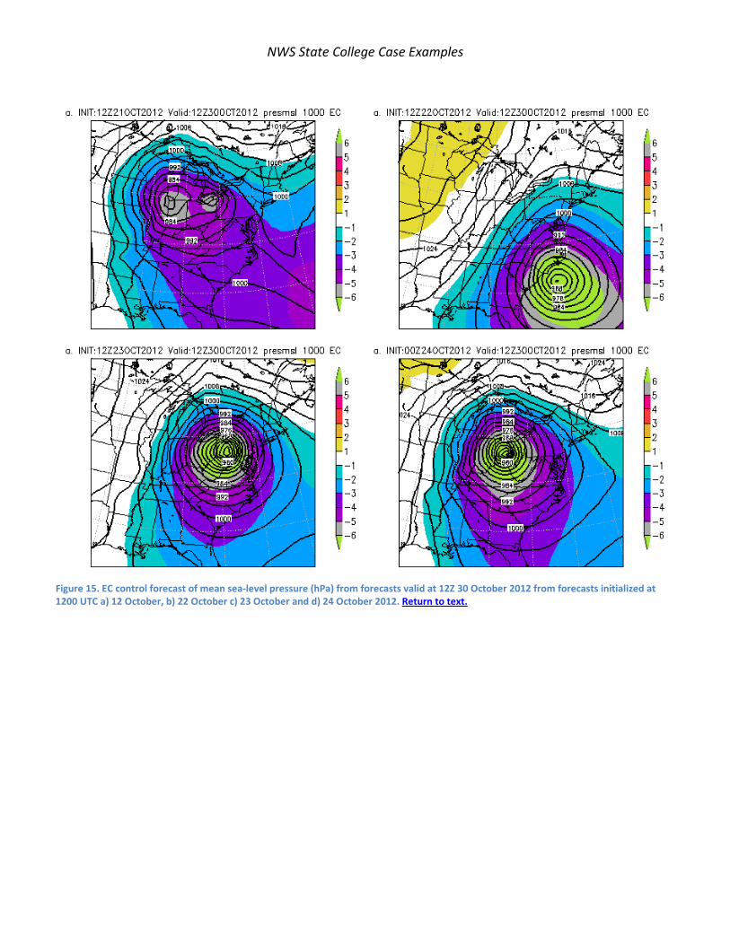
The best method to convey the forecasts is via ensembles as in addition to the pattern ensembles convey uncertainty information. However examing model run-to-run differences is sufficient to show the information regarding uncertainty. Figure 15 shows 4 EC pressure forecasts applying standardized anomalies valid at 1200 UTC 30 October 2012. Despite the storms intensity, the strength and location of the cyclone vary markedly from the 1200 UTC forecasts initialized at 1200 UTC 21, 22, 23 and 24 October 2012.

The impacts of the strong winds vary based on these forecasts as shown in Figure 16. The location of the strong 850 hPa winds, which include 6s wind anomalies vary markedly. Timing and location issues make the forecasts from the control run a moving target. The take-away message from the control run was an intense storm with considerable uncertainty with regard to timing, intensity and track.

NWS State College Case Examples

4.1.2 NCEP GFS Forecasts

GFS data had local storage and NOMADS retrieval limits. Forecasts from 6 successive 1200 UTC cycles from 23 to 28 October 2012. There was considerable run-to-run variation similar to the EC (Fig. 17). Unlike the EC, the GFS was slower to indicated the storm making the abrubt change in direction toward the East Coast of the United States

This impacts where the high winds would verify (Fig. 18) and the GFS showed areas of 6σ above normal 850 hPa winds which relative to the cases shown, would be devastating. The high winds along with the significant anomalies were good signals to consider strong and damaging winds at the surface.

4.1.3 GEF Forecasts

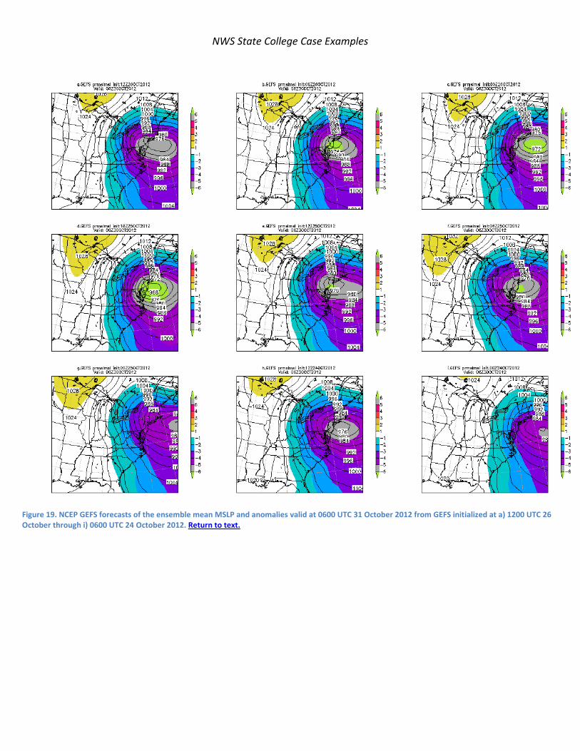
The changeable nature of these forecasts show the value of ensembles, which tend to be less changeable and have tools to highlight uncertainty. But for simplicity 9 GEFS runs are shown (Fig. 19) and all show a deep cyclone with a -5 to -6s cyclone coming onshore a few hour either side of 0600 UTC 30 October 2012. The most recent forecast in the ensemble mean has a weaker surface cyclone. The ensembles clearly show less variability then individual members. The 850 hPa winds in the GEFS also show a more tempered forecast. Likely the impact of uncertainty (Fig. 20).

5. Summary

Tropical storm Sandy will likely impact the East Coast of the United States between 29-31 October 2012. There is considerable uncertainty with respect to where the impacts will be most significant. The cyclone track, the cyclone intensity, and where the heavy rain and strong winds will verify is highly uncertain. The consensus in all forecasts is for a major cyclone with the potential to be an extreme high impact weather event. As the forecasts unfold the storm will be compared to previous storms of note. Several of these storms were shown here. Many contain interesting similarities and features. But each was unique. All of the historic comparative storms had significant standardized anomalies associated with them. The large standardized anomalies in these forecasts imply that this storm has a high likelihood of being an extreme high impact event. Hazel and the 26 November 1950 storm are likely good comparative storms. Hazel has been used a comparative storm to the forecasts of Sandy. It is a relatively good analog in that it involved a trough interaction, had strong u-wind anomalies and the storm moved to the west. However, the surface pressure and u-wind anomalies associated with Hazel were

NWS State College Case Examples

dramatically weaker than that forecast for Sandy. This would imply that Sandy has the potentially to be a higher impact storm than Hazel was in October 1954. Most of the deeper and high impact storms shared several characteristics including downstream blocking. The blocking likely contributed to the storm cutting off from the westerlies, slowing the forward progress and producing long and enduring periods of high winds, high seas, and heavy rainfall. Characteristics in the forecast associated with Sandy as it moves into the Mid-Atlantic region and southern New England coastal regions. More forecasts will be issued and as the forecast length decreases the skill will increase. Ensembles and probabilities will likely aid in making tempered but more useful forecasts. On Monday 29 October an estimated pressure of 943 hPa and an eye diameter of 20 nm was observed with 80kt winds and 100kt gusts around 1100 AM. The RAP pressure anomalies are shown in Figure 21. These data are every 3 hours from 0100 UTC through 1600 UTC 29 October. These data showed the 6σ pressure center in the analysis. 6. Acknowledgements Thanks to the EC TIGGE site for access to EC model, control and perturbation data. Thanks to the NWS NOMADS site of GFS data. All CFS and NCEP/NCAR data are from UCAR data site. NCEP produced the CFSR 30 year climate used. 7. References

Bodner, M. J., N. W. Junker, R. H. Grumm, and R. S. Schumacher, 2011: Comparison of atmospheric circulation patterns during the 2008 and 1993 historic Midwest floods. Natl. Wea. Dig., 35, 103-119.

Changnon S.A and J.M. Changnon 1992: Storm Catastrophes in the United States: Natural Hazards,6,2,93-107. DOI DOI: 10.1007/BF00124618

Doty, B.E. and J.L. Kinter III, 1995: Geophysical Data Analysis and Visualization using GrADS. Visualization Techniques in Space and Atmospheric Sciences, eds. E.P. Szuszczewicz and J.H. Bredekamp, NASA, Washington, D.C., 209-219.

Graham, Randall A., Richard H. Grumm, 2010: Utilizing Normalized Anomalies to Assess Synoptic-Scale Weather Events in the Western United States. Wea. Forecasting, 25, 428-445

Grumm, R.H. 2011: New England Record Maker rain event of 29-30 March 2010. NWA,Electronic Journal of Operational Meteorology,EJ4.

Grumm, R.H., and R. Hart, 2001a: Anticipating Heavy Rainfall: Forecast Aspects. Preprints, Symposium on Precipitation Extremes, Albuquerque, NM, Amer. Meteor. Soc., 66-70.

NWS State College Case Examples

Grumm, R.H. and R. Hart. 2001b: Standardized Anomalies Applied to Significant Cold Season Weather Events: Preliminary Findings. Wea. and Fore., 16,736–754.

Gyakum, JR , and E. S. Barker, 1988: A case study of explosive sub-synoptic scale cyclogenesis. Mon. Wea. Rev.,116, 2225–2253.

Hart, R. E., and R. H. Grumm, 2001: Using normalized climatological anomalies to rank synoptic scale events objectively. Mon. Wea. Rev., 129, 2426–2442.

Junker, N.W, M.J.Brennan, F. Pereira,M.J.Bodner,and R.H. Grumm, 2009:Assessing the Potential for Rare Precipitation Events with Standardized Anomalies and Ensemble Guidance at the Hydrometeorological Prediction Center. Bulletin of the American Meteorological Society,4 Article: pp. 445–453.

Kalnay, E., and Coauthors, 1996: The ncep/ncar 40-year reanalysis project. Bull. Amer. Meteor. Soc., 77, 437–471.

Ludlum, D. M., 1956: "The Great Atlantic Low". Weatherwise, 9, 64-65.

Knox, J.L., 1955: The Storm "Hazel", synoptic resume of its development as it approached Southern Ontario. Bull. Am. Meteor. Soc., 36, 239-246.

Saha, S., and Coauthors, 2006: The ncep climate forecast system. J. Climate, 19, 3483–3517. Saha, Suranjana, et. al., 2010: The NCEP Climate Forecast System Reanalysis. Bull. Amer. Meteor. Soc.,

BAMS,1015-1057. Stuart, N. and R. Grumm 2009, "The Use of Ensemble and Anomaly Data to Anticipate Extreme Flood Events in the Northeastern United States",NWA Digest,33, 185-202. Van Den Dool, H.M. 1994: Searching for analogues, how long must we wait. Tellus, 46A,314-324.

NWS State College Case Examples

Figure 1. NCEP/NCAR reanalysis data of the Hazel at 1800 UTC 15 October 1954. Data include a) 500 hPa heights (m) and standardized anomalies, b) 850 hPa winds (kts) and u-wind anomalies, c) precipitable water (mm) and standardized anomalies, and d) mean sea-level pressure (hPa) and pressure anomalies. Return to text.

NWS State College Case Examples

Figure 2. As in Figure 1 except for precipitable water viewed over the western Atlantic in 6-hour time steps from a) 1800 UTC 14 October 1954 through i) 1800 UTC 6 October 1954. Return to text.

NWS State College Case Examples

Figure 3. As in Figure 2 except for 500 hPa heights and height anomalies. Return to text.

NWS State College Case Examples

Figure 4. As in Figure 2 except of 850 hPa winds (contours) and u-wind standardized anomalies. Return to text.

NWS State College Case Examples

NWS State College Case Examples

Figure 5. As in Figure 2 except Climate forecast reanalysis data and CFSR climate showing conditions at 0000 UTC 31 October 1991. Return to text.

NWS State College Case Examples

Figure 6. As in Figure 5 except for 1200 UTC 31 October 1991 and over the western Atlantic. Return to text.

NWS State College Case Examples

Figure 7. As in Figure 1 except NCEP/NCAR reanalysis of precipitable water and precipitable water anomalies from a) 0000 UTC 01 December 1974 through i) 0000 UT December 1974. Return to text.

NWS State College Case Examples

Figure 8. As in Figure 7 except for mean sea-level pressure and pressure anomalies. Return to text.

NWS State College Case Examples

Figure 9. As in Figure 7 except for 850 hPa winds and u-wind anomalies. Return to text.

NWS State College Case Examples

Figure 10. NCEP/NCAR reanalysis data showing precipitable water and precipitable water anomalies from a) 1200 UTC 25 November through i) 1200 UTC 27 November 1950. Return to text.

NWS State College Case Examples

Figure 11. As in Figure 10 except for MSLP. Return to text.

NWS State College Case Examples

Figure 12. As in Figure 10 except for 500 hPa heights and height anomalies. Return to text.

NWS State College Case Examples

Figure 13. As in Figure 10 except for 850 hPa winds and u-wind anomalies. Return to text.

NWS State College Case Examples

Figure 14. CFSR data valid at 1200 UTC 29 March 1984. Return to text.

NWS State College Case Examples

Figure 15. EC control forecast of mean sea-level pressure (hPa) from forecasts valid at 12Z 30 October 2012 from forecasts initialized at 1200 UTC a) 12 October, b) 22 October c) 23 October and d) 24 October 2012. Return to text.

NWS State College Case Examples

Figure 16. As in Figure except for 850 hPa wind and u-wind anomalies. Return to text.

NWS State College Case Examples

Figure 17. NCEP GFS forecasts of MSLP and anomalies from 5 forecast cycles valid at 0000 UTC 30 October 2012 in 24 hour increments from forecasts initialized at a) 1200 UTC 23 October 2012 through e) 1200 UTC 28 October 2012. Return to text.

NWS State College Case Examples

Figure 18. As in 17 except for 850 hPa winds and wind anomalies. Return to text.

NWS State College Case Examples

Figure 19. NCEP GEFS forecasts of the ensemble mean MSLP and anomalies valid at 0600 UTC 31 October 2012 from GEFS initialized at a) 1200 UTC 26 October through i) 0600 UTC 24 October 2012. Return to text.

NWS State College Case Examples

Figure 20. As in Figure 19 except for GEFS ensemble mean 850 hPa winds and 850 hPa wind anomalies. Return to text.

NWS State College Case Examples

Figure 21. RAP mean sea level pressure (hPa) in 3-hour increments from a) 0100 UTC through b) 1600 UTC 29 October 2012. Return to text.

NWS State College Case Examples

Figure 22. As in Figure 21 except for RAP simulated reflectivity about the cyclone along the East coast. Return to text.

NWS State College Case Examples

Stations reporting wind gusts 50-59kt as of 1751 UTC (coolwx.com

• FDBB: UNKNOWN, [53kt, 27m/s] • KFMH: Otis Air National Guard Base, MA, United States [50kt, 25m/s] • KFOK: Westhampton Beach, The Gabreski Airport, NY, United States [51kt, 26m/s] • KFRG: Farmingdale, Republic Airport, NY, United States [50kt, 25m/s] • KJFK: New York, Kennedy Intl Arpt, NY, United States [57kt, 29m/s] • KMVY: Vineyard Haven, Marthas Vineyard Airport, MA, United States [51kt, 26m/s] • KUUU: Newport, Newport State Airport, RI, United States [51kt, 26m/s] • SCCI: Punta Arenas, Chile [51kt, 26m/s] • CWEF: Saint Paul Island Meteorological Aeronautical Presentation System, Canada [57kt, 29m/s] • KFOK: Westhampton Beach, The Gabreski Airport, NY, United States [51kt, 26m/s] • KFRG: Farmingdale, Republic Airport, NY, United States [50kt, 26m/s] • KHYA: Hyannis, MA, United States [50kt, 26m/s] • KISP: Islip, Long Island Mac Arthur Airport, NY, United States [52kt, 27m/s] • KJFK: New York, Kennedy Intl Arpt, NY, United States [57kt, 29m/s] • KMQE: East Milton, MA, United States [51kt, 26m/s] • KMVY: Vineyard Haven, Marthas Vineyard Airport, MA, United States [51kt, 26m/s] • KUUU: Newport, Newport State Airport, RI, United States [51kt, 26m/s]

NWS State College Case Examples

Greenport NY Monday 29 October 2012: