Nuclear Physics A493 (1989) 29-60

North-Holland, Amsterdam

WIGNER COEFFICIENTS FOR THE PROTON-NEUTRON

QUASISPIN GROUP:

An application of vector coherent state techniques

K.T. HECHT’

Pi~~sicr Department, University of Michigan, Ann Arbor, MI 48109, USA

Received 8 September 1988

Abstract: SO(S) 3 U(2) reduced Wigner coefficients, needed to extract the n, T-dependence of nuclear

matrix elements in the seniority scheme, are evaluated by vector coherent state techniques by

casting operators other than the group generators into their Bargmann z-space realizations. Results

are given, in terms of simple angular momentum recoupling coefficients and the K-matrix elements

of vector coherent state theory, for SO(S) couplings involving the 4., S-, and IO-dimensional

representations. Both a simplification of earlier results and a generalization to states of arbitrarily

high seniority has been achieved.

I. Introduction

In the past few years a generalized coherent state theory, termed vector coherent

state theory lm4), and its associated K-matrix technique ‘,‘) have been used to great

advantage to give very explicit matrix representations of many of the higher rank

symmetry algebras of interest in physical applictions. To date most of the detailed

applications have focused on the matrix representations, that is, on the matrix

elements of the generators of the algebras, [For a review and a more complete listing

of recent applications see ref. “).I The vector coherent state technique, however, is

in principle also a powerful tool for the detailed evaluation of the full Wigner-Racah

calculus of the higher rank algebras. This has been illustrated for the elementary

reduced-Wigner coefficients for U(n) which have been expressed ‘) in terms of

multiplicity-free U( n - 1) Racah coefficients and very simple K-matrix elements,

the normalization factors of the vector coherent state theory. More recently, Le

Blanc and Biedenharn “) have shown that some classes of SU(3),=, SU(2) reduced

Wigner coefficients are simple products of SU(2) 9-j coefficients and extremely

simple SU(3) K-matrix ratios. It is not yet completely clear to what extent the

spectacularly simple analytic form of such results can be generalized by means of

vector coherent state theory to the case of the most general SU(3) couplings,

particularly the cases involving outer multiplicities.

’ Supported in part by the US National Science Foundation

0375-9474/89/$03.50 Q Elsevier Science Publishers B.V.

(North-Holland Physics Publishing Division)

30 K.T. Hecht J Wigner coejkients

For this reason it may be useful to derive general expressions for the needed

Wigner coefficients of another simple example, with an SU(2) subgroup, the proton-

neutron quasispin group which is generated by an SO(5) 3 U(2) algebra, (or its

isomorphic Sp(4) algebra). Matrix representations of this algebra have been dis-

cussed previously in terms of vector coherent state theory ‘,‘). The development of

the proton-neutron quasispin formalism into a useful tool for the nuclear spectros-

copy of configurations of both protons and neutrons requires the explicit knowledge

of many SO(5) 1 U(2) reduced Wigner coefficients. With these the full n, T-depen-

dence can be extracted from nuclear matrix elements in the seniority scheme

(n = nucleon number, T = isospin). Although very explicit expressions have been

given previously ‘O,“) for the SO(5) reduced Wigner coefficients of many of the low

seniority representations of greatest interest in nuclear spectroscopy, a full analytic

solution to this problem had been hampered by a “missing quantum number

problem.” Vector coherent state theory and the associated K-matrix constructions

give an elegant solution to this problem in terms of the physically relevant coupling

scheme in which a state of seniority v and isospin T is constructed by coupling the

reduced isospin t of the u nucleons entirely free of J = 0 coupled pairs with the

resultant isospin T,, of the p pairs of nucleons coupled to J = 0, T = 1. The vector

coherent state construction in terms of this coupling scheme was discussed in ref. “).

It is the purpose of the present contribution to show how vector coherent state

techniques can be used to calculate the SO(5) 3 U(2) Wigner coefficients needed

for nuclear spectroscopy. In particular, Wigner coefficients for the coupling of

arbitrary irreducible representations with the 4-dimensional (spinor), 5dimensional

(vector) and lo-dimensional (regular) representations will be given in general

analytic form. Both a simplification and a complete generalization of the earlier

results “‘,“) has b een achieved, making it possible to treat representations of

arbitrarily high seniority.

The purpose of the present investigation is two-fold: One of the aims is a further

refinement and completion of an elegant tool of nuclear spectroscopy. A second

aim, however, involves the further development of the vector coherent state method

in its application to the Wigner-Racah calculus of higher rank algebras. It is hoped

that the techniques illustrated in some detail with the simple SO(5) 1 U(2) algebra,

involving mainly ordinary angular-momentum recoupling transformations, will also

prove useful in more challenging symmetries.

2. Vector coherent state realizations of the proton-neutron quasispin algebra

Vector coherent state theory takes its simplest form for algebras with the following

general structure: the generators of the algebra can be separated into a set of

commuting raising operators, their hermitian-conjugate lowering operators, and a

core subalgebra which contains the Cartan subalgebra of the full algebra. In its

SO(5) 2 U(2) version the proton-neutron quasispin algebra falls into this simple

K. T. Hecht / Wigner coeficients 31

category. Since normalization and phase factors are vital for the evaluation of Wigner

coefficients it will be important to give a careful definition of the various operators.

The raising operators are the J = 0, T = 1 pair creation operators defined by

A’(M,)=$C C (-l)‘~“‘a;,,,,,,,,aj-,,,,,,,l(:m,,qm,ZIIM,). (la) nt m,,

The hermitian-conjugate lowering operators are the J = 0, T = 1 pair annihilation

operators

A(MT) = (A.‘(&))‘. (lb)

The U(2) core subgroup is generated by the Cartan operator

H, =&,,.-(j+9=: c &,,,,a,,, ,,I, -(j+l) 3 (Ic) ,,>,*,

and the isovector generators, T, with standard spherical components

TLI = d C a~m,;a,,,,T;, To= !, c (&7+y,n,+~ - a;,,+,,,-;) . (IdI n, ,?I

(Note that a generalization to mixed configurations involving several j subshells is

immediate by including summations over bothj and m and the replacement (j +l) +

C (j+ A). Note also that To- H2.) It will also be useful to introduce Cartesian

components A:, A,, T,, (i = 1,2,3) defined in terms of the standard spherical

components, e.g., by A’(i1) = &(A~~* iA;), A’(O) = A:. SO(5) irreducible rep-

resentations are to be labeled by the Cartan highest weights, (w,w~),

W, =J’+;-;V, ml-t, (2)

where v and t are seniority and reduced isospin, (the isospin of the v nucleons

entirely free of J = 0 coupled pairs).

The single-nucleon creation and annihilation operators (for a fixed j, m) span the

4-dimensional irreducible representation (AA), while the 5-dimensional vector rep-

resentation (lo), and the IO-dimensional regular representation (11) are spanned

by the bifermion operators coupled to odd J(J,) and even J(J,), respectively; where

[a x a$]‘,,‘,,, = C C (.im,jm,)JM)(~m,,~m,~) TMT)ai,,l,,,,,,a:,,,,,,,~ ,,I, ,?a 1 m,, m,,

[a x a]& f IlI C (jm,.jm, 1 JW(im,,im,L 1 TM,) m, ?P) m,, n1,2

x aj- )),, _,,,,,(-I)’ -“‘l’- I WI ” a,p,,*,~,,, J-1) I_ ~~5+~?~~52

[a: x a]& 5% C C (jm,jm,)JIM)(~m,,~m,~) TM,) t*, , vz- m,, ,IIf2

xa’ ,nl,,n,,a,~m2-,n,, (_I), -wll+l-J-,,

(3)

The relationship among standard SO(5) irreducible operators, Tz,I;“;i,, can be given

through the matrix elements of the generators, e.g.

[A%%), %‘,$,,I

=;, T~~i..,,+,,,,((w,t)H,+1T’M,+M,,lA+(M,,)l(w,t)H,TM,). (4)

32 K.T. Hecht / Wigner coefficients

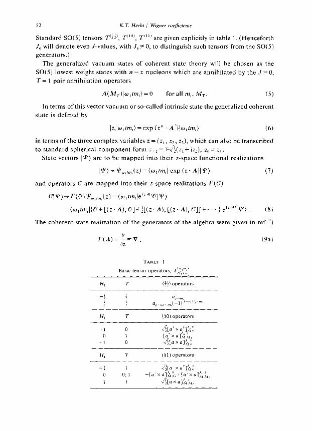
Standard SO(S) tensors T’i i’ T”O’ , T”” are given explicitly in table 1. (Henceforth

J, will denote even J-values,‘with J, # 0, to distinguish such tensors from the SO(5)

generators.)

The generalized vacuum states of coherent state theory will be chosen as the

SO(5) lowest weight states with n = u nucleons which are annihilated by the J = 0,

T = 1 pair annihilation operators

A(&)l~tm,)=O for all m,, MT. (5)

In terms of this vector vacuum or so-called intrinsic state the generalized coherent

state is defined by

Iz, qtm,)= exp (z* . At)(w,tm,) (6)

in terms of the three complex variables z, = (z,, z2, z,), which can also be transcribed

to standard spherical component form z,, = F&Z, + izz), z,, = z3.

State vectors IP) are to be mapped into their z-space functional realizations

I W + qu,tm,(z) = (w, tm,l exp (z * Al W (7)

and operators 6 are mapped into their z-space realizations r(0)

S\U)+ T(6)1Yw,,m,(~) =(~,tm,\e(~‘~)D[ %?)

=(~,tm,({B+[(z~A),B]+~[(z~A),[(z~A),0]]+~~~}e’”‘~‘(~). (8)

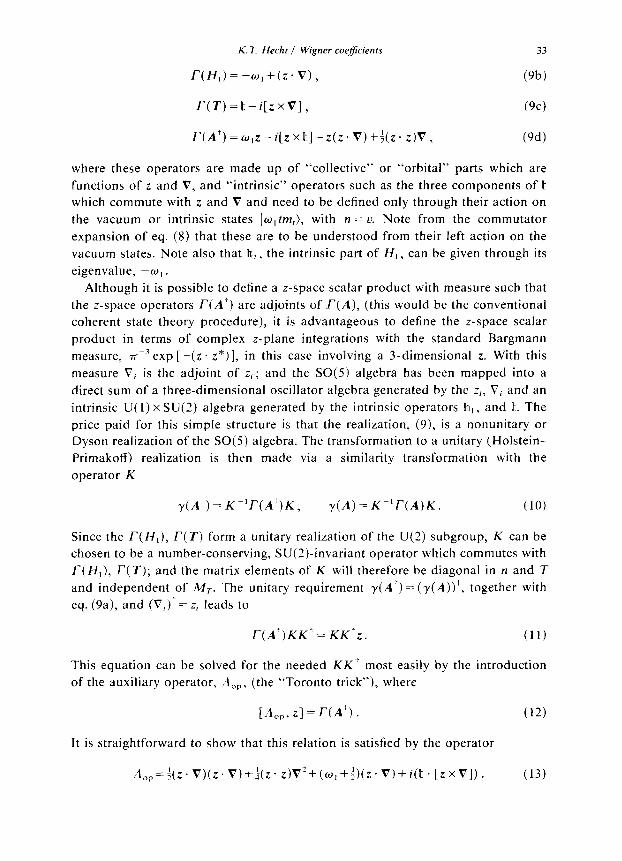
The coherent state realization of the generators of the algebra were given in ref. ‘)

T(A) =&7 az ’

@a)

TABLE 1

Basic tensor operators, T:y,‘F,;’ /

HI i- (44) operators

(IO) operators

+1

0 -1

HI

+I

0

-1

0 J[atx .+]j:; 1 [a’ x a]‘; yv, 0 &[a x Q]“G :;

T (I 1) operators

I &[Q x a+]J*:;

0; 1 -[a’ x Ll1-L::; +[a+x Ll]‘; t,

1 A[ a x n].‘& ‘v,

K. T. Hechr / Wigner coejkiicients 33

l-(I-f,)=-w,+(z.V), (9b)

T(T)=It-i[zxV], (9c)

T(A’)=w,z-i[zxk]-z(z. V)+$(z. z)V, (9d)

where these operators are made up of “collective” or “orbital” parts which are

functions of z and V, and “intrinsic” operators such as the three components of It

which commute with z and V and need to be defined only through their action on

the vacuum or intrinsic states ]w,fm,), with n = ZI. Note from the commutator

expansion of eq. (8) that these are to be understood from their left action on the

vacuum states. Note also that On,, the intrinsic part of H,, can be given through its

eigenvalue, -w, .

Although it is possible to define a z-space scalar product with measure such that

the z-space operators T(A.‘) are adjoints of T(A), (this would be the conventional

coherent state theory procedure), it is advantageous to define the z-space scalar

product in terms of complex z-plane integrations with the standard Bargmann

measure, Y3 exp [-(z. z”)], in this case involving a 3-dimensional z. With this

measure Vi is the adjoint of z,; and the SO(5) algebra has been mapped into a

direct sum of a three-dimensional oscillator algebra generated by the zi, V, and an

intrinsic U(1) xSU(2) algebra generated by the intrinsic operators On,, and e. The

price paid for this simple structure is that the realization, (9), is a nonunitary or

Dyson realization of the SO(5) algebra. The transformation to a unitary (Holstein-

Primakoff) realization is then made via a similarity transformation with the

operator K

y(A+) = K’T(A.‘)K, y(A) = K-‘T(A)K. (10)

Since the T(H,), T(T) form a unitary realization of the U(2) subgroup, K can be

chosen to be a number-conserving, SU(2)-invariant operator which commutes with

Z’(H,), I’(T); and the matrix elements of K will therefore be diagonal in n and T

and independent of MT. The unitary requirement y(AT) = (y(A))+, together with

eq. (9a), and (V,)“= z, leads to

l-(A’)KK’= KK’z. (11)

This equation can be solved for the needed KK.’ most easily by the introduction

of the auxiliary operator, Aor,, (the “Toronto trick”), where

[&“, z,] = I-( A-‘-) . (12)

It is straightforward to show that this relation is satisfied by the operator

n,,=~(z~V)(z’V)+~(z~z)V’+(w,+~)(z~V)+i(t~[zxV]). (13)

34 K. T. Hecht / Wigner coejicients

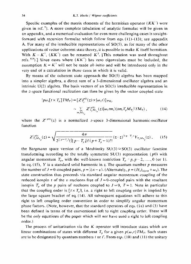
Specific examples of the matrix elements of the hermitian operator (KK ‘) were

given in ref. ‘). A more complete tabulation of analytic formulae will be given in

an appendix, and a numerical evaluation for even more challenging cases is straight-

forward with recursion formulae which follow from eqs. (ll)-( 13); see appendix

A. For many of the irreducible representations of SO(5), as for many of the other

applications of vector coherent state theory, it is possible to make K itself hermitian.

With K = K ‘, (KKt) can be renamed K’. [This notation was used throughout

refs. “V’).] Since cases where (KK’) has zero eigenvalues must be included, the

assumption K = Kt will not be made ab initio and will be introduced only in the

very end of a calculation in those cases in which it is valid.

By means of the coherent state approach the SO(5) algebra has been mapped

into a simpler algebra, a direct sum of a 3-dimensional oscillator algebra and an

intrinsic U(2) algebra. The basis vectors of an SO(5) irreducible representation in

the z-space functional realization can then be given by the vector coupled state

where the Z(““)(z) is a normalized z-space 3-dimensional harmonic-oscillator

function

Z(PW T,,Mr ,,w= J,. - 4r :(p sJ(;[p-T,])!(p+T,+l)!!

(z’ Z)l’P-T”YT,,Ms ,,(z) , (15)

the Bargmann space version of a Moshinsky SU(3) =~S0(3) oscillator function

transforming according to the totally symmetric SU(3) representation (PO) with

angular momentum T,, with the well-known restriction T,, = p, p - 2,. . . ,O (or 1).

In eq. (15), Y is a standard solid harmonic in z. The quantum number p measures

the number of J = O-coupled pairs, p = t( n - II). (Alternately, p = (H,)eigen + 0,). The

state construction thus proceeds via standard angular momentum coupling of the

reduced isospin t of the u nucleons free of J = O-coupled pairs with the resultant

isospin T,, of the p pairs of nucleons coupled to J = 0, T = 1. Note in particular

that the coupling order is [t x T,], i.e. a right to left coupling order is implied by

the large square bracket of eq. (14). All subsequent equations will adhere to this

right to left coupling order convention in order to simplify angular momentum

phase factors. (Note, however, that the standard operators of eqs. (la) and (3) have

been defined in terms of the conventional left to right coupling order. These will

be the only equations of the paper which will not have used a right to left coupling

order.)

The process of unitarization via the K operator will introduce states which are

linear combinations of states with different Tp for a given p(w, t) TMT. Such states

are to be designated by quantum numbers i or i’. From eqs. (10) and (11) the unitary

K.T. Hechr / Wigner coejicients

z-space operator can be put in the form

y(A’) = K’z(K”)-’ ,

leading to the angular momentum reduced matrix element

35

(16)

(n+2(w,t)T’i’((y(A+)lln(w,t)Ti)

=TjFT (K')i'T,:(P+lwl[tx T~lT'IIZIIPwI[tx TplT)((K”)-‘)Tri i’

=(n+2(w,t)T’i’llA’lln(co,t)Ti). (17)

The reduced matrix element ofthe operator z is given by standard angular momentum

coupling theory

t T, T

(p+lw,[tx T;]T’ljzjlpw,[tx T,]T)== 0 1

i 1 1 (Tbllzll T,) t T; T’

= u(tT,T’l; ~bNT:,IlzIIT,), (18)

where the 3-dimensional oscillator reduced matrix element is given in terms of a

simple SU(3) 3 SO(3) reduced Wigner coefficient

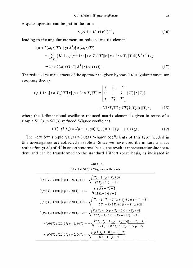
(T:,IIzIIT,)=JT;+~((PO)T~; (lo)1 ll(~+l,O)T;). (19)

The very few simple SU(3) 3 SO(3) Wigner coefficients of this type needed in

this investigation are collected in table 2. Since we have used the unitary z-space

realization y(A.‘) of A-t in an orthonormal basis, the result is representation-indepen-

dent and can be transformed to the standard Hilbert space basis, as indicated in

TAHLE 2

Needed SU(3) Wigner coeficients

((pO)T,,;(2O)O)j(p+2,0)7,,)= (p+7Y’+3)(p-q,+2) 3(p+l)(p+2)

36 K.T. Hecht / Wigner coeficients

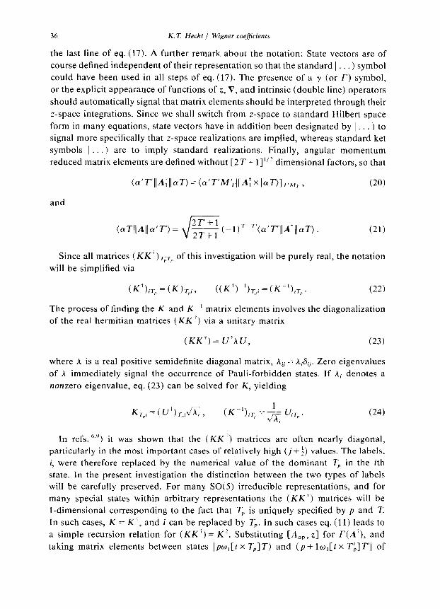
the last line of eq. (17). A further remark about the notation: State vectors are of

course defined independent of their representation so that the standard 1 . . . ) symbol

could have been used in all steps of eq. (17). The presence of a y (or I’) symbol,

or the explicit appearance of functions of z, V, and intrinsic (double line) operators

should automatically signal that matrix elements should be interpreted through their

z-space integrations. Since we shall switch from z-space to standard Hilbert space

form in many equations, state vectors have in addition been designated by 1 . . . ) to

signal more specifically that z-space realizations are implied, whereas standard ket

symbols 1 . . ) are to imply standard realizations. Finally, angular momentum

reduced matrix elements are defined without [2T+ 1]“2 dimensional factors, so that

(aT(IAllcu’T’) = (21)

Since all matrices (KK ‘) T,,:T,, of this investigation will be purely real, the notation

will be simplified via

CKi-)iT,, = CK)T,,t T ((K+)~'),,,i=(K-'),,,,. (22)

The process of finding the K and K -’ matrix elements involves the diagonalization

of the real hermitian matrices (KK ‘) via a unitary matrix

(KK+)= U’AU, (23)

where A is a real positive semidefinite diagonal matrix, A, = ~~6,. Zero eigenvalues

of A immediately signal the occurrence of Pauli-forbidden states. If A, denotes a

nonzero eigenvalue, eq. (23) can be solved for K, yielding

K,,,, = ( u+) ~,,rfi , 1

CK-I),,, =~;i; uir,, .

In refs. 6,9) it was shown that the (KK.‘) matrices are often nearly diagonal,

particularly in the most important cases of relatively high (j +i) values. The labels,

i, were therefore replaced by the numerical value of the dominant T, in the ith

state. In the present investigation the distinction between the two types of labels

will be carefully preserved. For many SO(5) irreducible representations, and for

many special states within arbitrary representations the (KK.‘) matrices will be

l-dimensional corresponding to the fact that T, is uniquely specified by p and T.

In such cases, K = K.i, and i can be replaced by T,. In such cases eq. (11) leads to

a simple recursion relation for (KK.‘) = K 2. Substituting [A,, , z] for T(A’), and

taking matrix elements between states IpwI[ t x T,]T) and (p + lw,[ t x Tb] T’( of

K.T. He&t / Wiper coe&cients

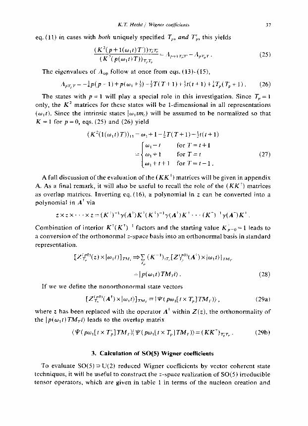
eq. (11) in cases with both uniquely specified T,, and Tb, this yields

(K’(p+l(w,t)T’))T,:~:=.

(Kz(p(w,~)T))T,,T,, ‘-“k7- p+ 1 q;-f

The eigenvalues of &r follow at once from eqs. (13)~(15),

37

(25)

A PT,>T = +(p-l)+p(w,++~T(T+l)+~t(t+l)+~T,(Tp+l). (26)

The states with p = 1 will play a special role in this investigation. Since T, = 1

only, the K’ matrices for these states will be l-dimensional in all representations

(w,t). Since the intrinsic states Iw,tm,) will be assumed to be normalized so &hat

K = 1 for p = 0, eqs. (25) and (26) yield

(E?(l(w,t)T)),,=w,fl-;T(T+l)+$t(t+l)

1

u,--t for T=t+l

= w,+1 for T= t (27) w,+t+1 for T=t-1.

A full discussion of the evaluation of the (TM.‘) matrices will be given in appendix

A. As a final remark, it will also be useful to recall the role of the (KK’) matrices

as overlap matrices. Inverting eq. (16), a polynomial in z can be converted into a

polynomia1 in At via

ZXZX’. .xz=(K+)-‘r(A’)K’(K’)-‘ye+.. .(K+)-‘y(A’)K’.

Combination of interior K’( K’))’ factors and the starting value Ki+ = 1 leads to

a conversion of the orthonormal z-space basis into an orthonormal basis in standard

representation.

VT;“‘(z) x I~,~)1 TM, *;, (K-‘),T,,[G$“(A’) XI~I~>ITM,

= IfJ(fU,t)Tbf,i). (28)

If we we define the nono~hono~al state vectors

CZy,“(& x 1% t)ITM, =l~(~,lfx 7;,lT&H, (294

where z has been replaced with the operator At within Z(z), the orthonormality of

the Ip(w, t)TM,i) leads to the overlap matrix

(*(P,[~x T~IT~T)I~(~~,[~x T,ITMT))=(K~‘~T,;T,, . (29b)

3. Calculation of SO(5) Wiper coefficients

To evaluate SO(5) =) U(2) reduced Wigner coefficients by vector coherent state

techniques, it will be useful to construct the z-space realization of SO(5) irreducible

tensor operators, which are given in table 1 in terms of the nucleon creation and

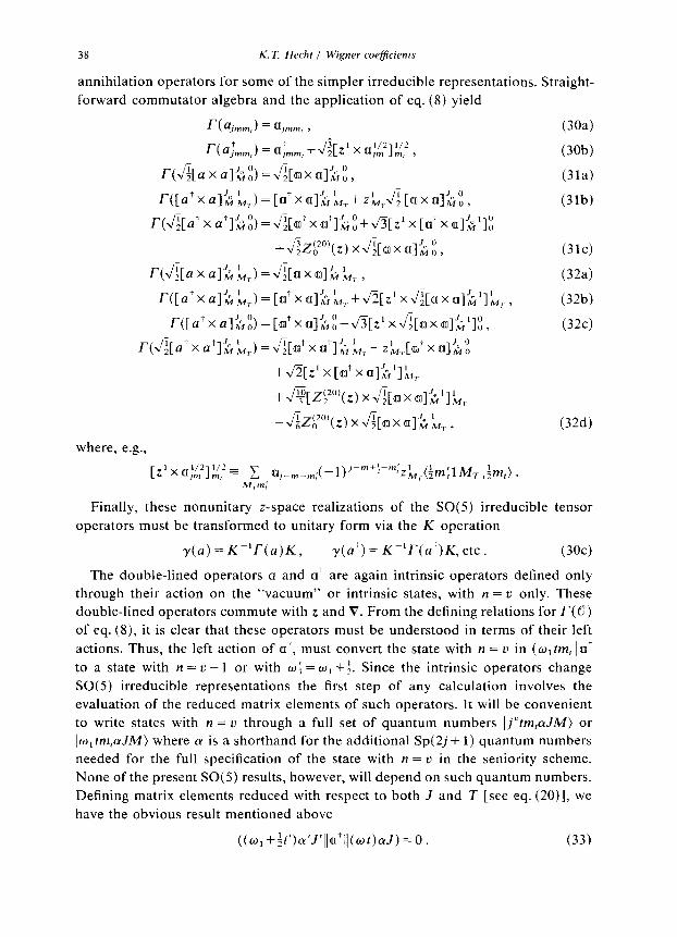
38 K. T. Hecht / Wiper coeficients

annihilation operators for some of the simpler irreducible representations. Straight-

forward commutator algebra and the application of eq. (8) yield

r(ajmm,) = a~n,,m, 3 (joa)

r(ujmm,)=aO:mm,+J~[Z~XQ:~]fn/,2, (Sob)

T(J[axa]~p,)=J[eoxan]~:,, (31a)

r([a+xa]hf, ,)=[aiXa]J~~T+z'M, &mxa]f& (31b)

T(J~[a'xa']~~)=J~[anixan:]~0,+J5[z'x[ao+xan]~']~

+Jz~~)(z)xJ[~xx]~::, (31c)

r&J x a]h ‘,,) =&an x an& a, , (32a)

r([a’x a]h ;,, = [ an+x0]~~,+JZ[z’xJ[aoxan]~‘]‘,,, (32b)

r([a+xa]~~)=[an’xan]~~-~[2’xJ~[anxan]~’]~, (3.2~)

r(J~[a’xai]~~,)=J~[an+xo’]~a,-z~,[a;o’xsn]X::

+Jz[z’x[an+xa]f$]ar

+~~[z:z”‘(z)xJIQx~]~‘]l,i

-Jbzb*“‘(z)x\/~[axan]~~r, (32d)

where, e.g.,

[z’x~~~*]~,2~~~~~~j-m-m;(-l)~~“‘+:~”;Z~,(tm:lM,~~m,).

Finally, these nonunitary z-space realizations of the SO(5) irreducible tensor

operators must be transformed to unitary form via the K operation

r(a) = KPIT(a)K, -y(a’) = IC’T(a’)K, etc. (3Oc)

The double-lined operators o and at are again intrinsic operators defined only

through their action on the “vacuum” or intrinsic states, with n = u only. These

double-lined operators commute with z and V. From the defining relations for I-( 0’)

of eq. (8), it is clear that these operators must be understood in terms of their left

actions. Thus, the left action of ot, must convert the state with n = ZI in (w, tm, 1 at

to a state with n = u - 1 or with W: = w, +i. Since the intrinsic operators change

SO(5) irreducible representations the first step of any calculation involves the

evaluation of the reduced matrix elements of such operators. It will be convenient

to write states with n = u through a full set of quantum numbers Ij’tm,aJM) or

lw,tm,cyJM) where (Y is a shorthand for the additional Sp(2j-t 1) quantum numbers

needed for the full specification of the state with n = u in the seniority scheme.

None of the present SO(S) results, however, will depend on such quantum numbers.

Defining matrix elements reduced with respect to both J and T [see eq. (20)], we

have the obvious result mentioned above

((w,+~t’)cu’J’lla+lI(wt)cuJ) =o. (33)

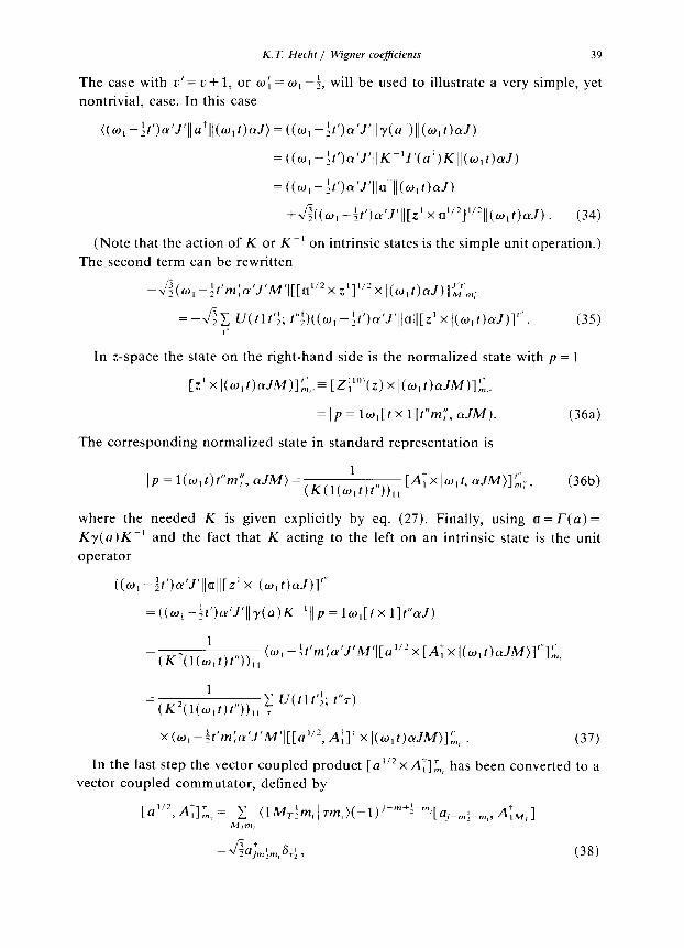
K. T Hecht / Wigner coejj’icients 39

The case with u’= u + 1, or CO{ = w, -f, will be used to illustrate a very simple, yet

nontrivial, case. In this case

((CO, -~t’)~‘J’lla+ll(w,r)~~) = ((CO, -tt’)~‘J’Ilr(a’)ll(W,t)(YJ)

= ((w, -;t’)cr’J’I]K’T(ai)K ]l(w,t)CXJ)

= ((CO, -~t’)(Y’J’IIQOi-Il(W,t)aJ)

+J&O, -;f’)LY’J’]][Z’X60”‘]“2]](w,t)cuJ). (34)

(Note that the action of K or Km’ on intrinsic states is the simple unit operation.)

The second term can be rewritten

-&CO, -;f’m:cr’J’M’([[o”*x z’]“Z x ](&J,t)LrJ)]$:,;

=-J$ U(t1r’i; t”)(( w, -$‘)a’J’llblll][z’ x ](w,f)aJ)]“‘. (35) I”

In z-space the state on the right-hand side is the normalized state with p = 1

[z’ X ](CiJ,t)cuJM)]:,,,= [z:““(z) X ](w,t)aJM)]::~

= Ip = lw,[t X l]Z”rn:‘, CrJM). (36a)

The corresponding normalized state in standard representation is

where the needed K is given explicitly by eq. (27). Finally, using (III = T(a) =

Ky(a)K-’ and the fact that K acting to the left on an intrinsic state is the unit

operator

((CO, -:t’)a’J’]ldll][Z’x ](w,t)CYJ)]“’

=((w,-~t’)~~‘J’~~y(a)K~‘]~p=lw,[txl]t”c~J)

1

=(K’(l(w,t)t”)),, (w, -$t’m:a’J’M’][~“~ x [A; x ~(w,t)aJM)]“‘];>,

1

x(w,-~t’m:cu’J’M’l[[u”*,A:]‘xl(w,t)aJM)]~, . (37)

In the last step the vector coupled product [a”* x AT];, has been converted to a

vector coupled commutator, defined by

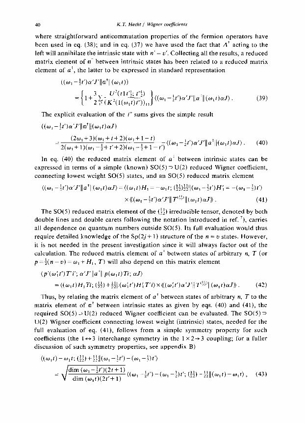
40 K.T. Hecht / Wigner coeficients

where straightforward anticommutation properties of the fermion operators have

been used in eq. (38); and in eq. (37) we have used the fact that At acting to the

left will annihilate the intrinsic state with n’ = u’. Collecting all the results, a reduced

matrix element of ot between intrinsic states has been related to a reduced matrix

element of a’, the latter to be expressed in standard representation

= 1+3x 1 U2(t1t’+; G) 2 I” (K2(l(o,t)t”)),, I

((w, -~tl)(Y)Jflla+ll(o,t)(YJ). (39)

The explicit evaluation of the t” sums gives the simple result

((0, -~t’)(Y’/‘i(an+ll(w,t)aJ)

(2w, +3)(w, + t +2)(w, + 1 - t)

= 2(0, + l)(w, -$+ t’+2)(w, -f+ 1 -t’) ((w, -~r’)(r’J’lla;ll(w,t)cYJ). (40)

In eq. (40) the reduced matrix element of LX+ between intrinsic states can be

expressed in terms of a simple (known) SO(5) 1 U(2) reduced Wigner coefficient,

connecting lowest weight SO(5) states, and an SO(5) reduced matrix element

((w, -~t’)a’J’llaill(W,t)(YJ) =((w,t)H, = -o,t; (&ll(wl -$)H; = -(w, -$)t’)

x (((w, -$‘)&r’IJ T’::‘Il(w,t)aJ)). (41)

The SO(5) reduced matrix element of the ($4) irreducible tensor, denoted by both

double lines and double carets following the notation introduced in ref. ‘), carries

all dependence on quantum numbers outside SO(5). Its full evaluation would thus

require detailed knowledge of the Sp(2j + 1) structure of the n = z, states. However,

it is not needed in the present investigation since it will always factor out of the

calculation. The reduced matrix element of a’ between states of arbitrary n, T (or

p = $( n - u) = w, + H, , T) will also depend on this matrix element

(p’(w;t’)T’i’; a’J’llutllp(w,r)Ti; d)

=((co,t)H,Ti; (~~)+~~~~(~~r’)H~T’i)x(((o~r’)cw’J’~(T’~~’~/(w,r)~J)). (42)

Thus, by relating the matrix element of ui- between states of arbitrary n, T to the

matrix element of oli between intrinsic states as given by eqs. (40) and (41), the

required SO(5) 2 U(2) reduced Wigner coefficient can be evaluated. The SO(5) 2

U(2) Wigner coefficient connecting lowest weight (intrinsic) states, needed for the

full evaluation of eq. (41), follows from a simple symmetry property for such

coefficients (the l-3 interchange symmetry in the 1 x 2* 3 coupling; for a fuller

discussion of such symmetry properties, see appendix B)

((w,r)--w,r; (~~)+~~ll(o,-or’)-((w,-_f)r’)

= J dim(01-fr’)(2r+1)((W,-fr~)_(W,-f)rf; (U)-Ul\(o,r)_w,r), (43) dim (o,r)(2r’+ 1)

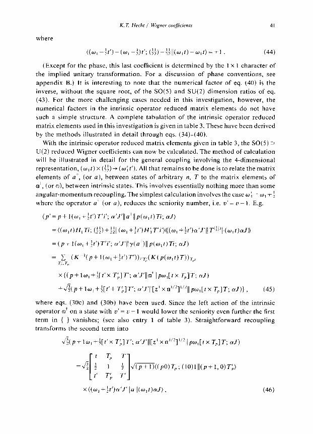
K. T. Hecht / Wigner coefficients 41

where

((co-;t’)-(W,-;)f’; (ff)-~~lI(w,t)-wlt)=+l. (44)

(Except for the phase, this last coefficient is determined by the 1 x 1 character of

the implied unitary transformation. For a discussion of phase conventions, see

appendix B.) It is interesting to note that the numerical factor of eq. (40) is the

inverse, without the square root, of the SO(5) and SU(2) dimension ratios of eq.

(43). For the more challenging cases needed in this investigation, however, the

numerical factors in the intrinsic operator reduced matrix elements do not have

such a simple structure. A complete tabulation of the intrinsic operator reduced

matrix elements used in this investigation is given in table 3. These have been derived

by the methods illustrated in detail through eqs. (34)-(40).

With the intrinsic operator reduced matrix elements given in table 3, the SO( 5) 1

U(2) reduced Wigner coefficients can now be calculated. The method of calculation

will be illustrated in detail for the general coupling involving the 4-dimensional

representation, (w,f) x (l:) + (w; t’). All that remains to be done is to relate the matrix

elements of a’, (or a), between states of arbitrary n, T to the matrix elements of

ali, (or an), between intrinsic states. This involves essentially nothing more than some

angular-momentum recoupling. The simplest calculation involves the case CIJ{ = w, + 5

where the operator at (or a), reduces the seniority number, i.e. Y’ = u - 1. E.g.

(p’=~+l(w,+$t’)T’i’; a’J’lla+llp(w,t)Ti; d)

=((w,t)H,Ti; (~~)+~~~~(W,+~~‘)H;T’~‘)(((~,+~~’)(Y’J’IIT’:~’IJ(~,~)LYJ))

=(p+l(w,+$t’)T’i’; Lu’J’lly(ui)llp(w,r)Ti; ad)

= T,FT (Km’(p+l(w,+ft’)T’))i~~,:(K(p(w,t)T))~,,, P

x{(p+lw,+f[t’x T;]T’; a’J’~~an~~pcw,[tx T,]T; aJ)

+&p+lw,+;[r’+T;]T’; a’J’J~[z’~an’~]“~~lpw,[tx TJT; cd)}, (45)

where eqs. (30~) and (30b) have been used. Since the left action of the intrinsic

operator or- on a state with v’ = v - 1 would lower the seniority even further the first

term in { } vanishes; (see also entry 1 of table 3). Straightforward recoupling

transforms the second term into

&~+lw,+;[t’x T;]T’; a’J’([[z’ x ~n”~]“~Ij pw,[ t x T,]T; cd)

x((W,+tt’)(Y’J’lluIl(w,t)(yJ)) (46)

42 K. T Hecht / Wigner coeficients

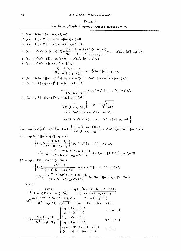
TABLE 3

Catalogue of intrinsic-operator reduced matrix elements

5. ((0,+:t’)n’J’J~~~~(w,t)uJ)=((w,+tt’)a’J’llall(w,f)uJ) 6. ((co1 -ft’)a’.+l~p = lw,[t X I]t”cd)

3 =J U(t1 t’& 1”:)

2 (KYl(w,t)t”))l, ((w, -~t’)u’,‘lla+ll(w,t)cuJ)

1

(K*(l(qt)t’)),, ((W,t’)a’_q[a+x a]‘*,‘~I(w,t)aJ)

9. ((O,fl)N)JIIIJI[QX~]‘c’IJP= 1u,[rx I]f”d)

x ((@.I, t’)a’J’ll[a >X a].‘J’ll(w, t)a_Q?i,.,

+JZU(tll’l; t”l)((w,t’)n’J’ll[a+x~].‘~‘~~(~,t)~~) I 11. ((w,t’)u’J’li[bli’xQ]J~‘i/(W,f)nJ)

= l-+22: 1 U’(tlt’l; 1”l)

,I’ (K’(l(w,t)t”)),, 1 ((w,t’)a’/‘ll[n’ xa]J~‘l(w,t)cuJ)

+A?,,, r: (-1) ‘+‘-“‘xqFFi-)u(ll?l; t”1)

(K’(l(w,t)t”)),,v’(2r+I) ((w,t)cu’.q[a+x a]q(w,tfd)}

I’

= 1+‘y {

(21”fl)

,~‘(2r+l)(K2(l(w,r)t”)),, ((W,t)CY’J’ll[alxa].‘l”il(wlt)aJ)

+&;T: C-1) ‘+~-‘“~U(tltl; t”l)

,” (K’(l(w,t)t”)),,~ ((Co, t)tu’J’l)[at x n]‘*‘ll(wl t)d)

where

l+E (21”+ 1) (W,+1)~(~,+~)-_(~~,+2)f(t+l)

,“(2t-t.l)(K”(l(o,+l)“t”)),,= (w,-t)(w,+l)(w,+t+l)

1+2x U2(tlt’l: PI) (w,+2)(w,+2+tl

= I, ,“(K?(l(W,t)f ))I,

i

(w, + l)(W, + 1+ I) fort’=r-1

w,(w,+2)‘-(w,t-l)t(t~l)

(o,-t)(w,+l)(o,+t+l) for I’ = t

K. iY Hecht / Wigner coeficients 43

where eq. (19) and entry 5 of table 3 have been used for the reduced matrix elements

of z and CL Note that eq. (19) could also be expressed through the useful identity

[z’ x z~(‘Yz)lq;Mi,, = -+t;,~ ‘“+““‘(z)~((po)T,; (lO)lll(p+ l,O)Tb). (19’)

Finally,

where the SO(5) Wigner coefficient connecting intrinsic (or SO(5) lowest weight)

states has the simple value +l. The combination of eqs. (45)-(46) gives the wanted

SO(5) 3 U(2) Wigner coefficient which is writen explicitly as the first energy of table

4. Note that this Wigner coefficient is given solely by the K-matrix elements of

vector coherent state theory, a very simple 3-dimensional oscillator coupling

coefficient, and an ordinary angular momentum 9-j recoupling coefficient, given

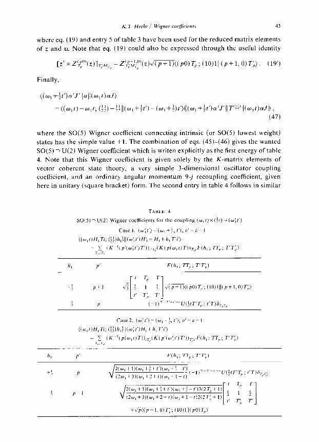
here in unitary (square bracket) form. The second entry in table 4 follows in similar

TAISLF. 4

SO(S) 1 U(2) Wigner coefficients for the coupling (w, t) x ($4) + (CO; t’)

Case]. (w;t’)=(w,+~,t’);u’=u~l

((w,t)H,Ti; (;:)h,:ll(w;t’)H’,= H,+h,T’i’)

= ,F, (K ‘(P’(wlt’)T’)),.,,:(K(P(w,t)T)),,,,F(h,; n,,; T’T;,) / /,

h, P’ F(h, ; 7-T,, ; T’T;,)

Case2. (w’,t’)=(w,-i,t’);u’=u+l

((w,t)H,Ti; (;f)h,fIl(w;t’)H,+ h,T’i’)

= r, (K~‘(p(w,t)T)),,~,(K(P’(wlt’)T’)),~:, F(h,; n,,; T’T;,) lil. 1,;

h, P’ .?/I, ; 7-q ; 7-T;,)

+f 2(w,+l)(w,+~+t’)(w,+i-t’)

P J(2w,+3)(~,+2+t)(w,+l_t) (-1)‘~“+‘~‘U(~tT’T,,;t’T)61~,,,;

f T,, 7- I

p-1 2(w,+l)(w,+~+t’)(w,+~-t’)3(27-,,+l) , (2w,+3)(w,+2+t)(w,+lLt)2(2T;,+l) ;, ;,

[ I i

,’ T’

44 K. T. Hecht / Wigner coeficients

fashion from the reduced matrix element of a. Since, r(a) = Q, contains but a single

term, and p’= p in this case, the recoupling process is even simpler and leads to an

expression involving an ordinary Racah coefficient given here in U-coefficient that

is again in unitary form.

Coefficients for wi = w, -$ for which a’ (or a) increases the seniority number

from ~1 to u’= v-t 1, can be obtained in their simplest form from the coefficients

with w; = w, + $ and the l-3 interchange symmetry property for such coefficients

((m,t)H,Ti; ($$)h$ll(~,-+t’)H;T’i’)

-h~l/(~,t)H,Ti) (48)

(see also appendix B). With the renaming To T’, t++ t’, and the use of simple

symmetry properties of the recoupling coefficients these can be put into the simple

form given in table 4.

Although coefficients for w ; = w, -4 can be obtained in their simplest form from

this symmetry property they can also be evaluated directly by the techniques outlined

above. Thus, e.g.

(p’=p--l(w,-+t’)T’i’; a’J’]]a]lp(w,t)Ti; (YJ)

x (p - lw, -;[t x T;]T’; cr’J’IIaIIpw,[t x T,]T; cd) (49)

again with the use of eqs. (30~) and (30a). Although care must be taken to define

the reduced matrix element of o through its left action (see entry 6 of table 3) we

will find it more convenient to perform the angular momentum recoupling on the

right through prior hermitian conjugation, and use

(P-lw,-+[t’x T;]T’; a’J+mj$m,[tx T,]T; d)

J+,pJ’+T+:-T’ =(-1) - J

(2J+ 1)(2T+ 1)

(2Y-t 1)(2T’+ 1)

x(pw,[tx T,]TM,; (~JMI[anj:x[Z~~‘,“(z)xl(w,-it’); a’J’)]“];;,

= (-1) J+j-J’+T+;mT’ dz; (_l)~-~‘+,‘~,“U(~t’TTb; ,uT!)

x(pw,[tx T,]TM,I[Z~~‘,‘(z)x[z’x/o,t)]“‘]~~

x(p= 1w,[tx 1]t”; aJ(]a$;l](w,-it’); (Y’J’)*) (50)

K.T. Hecht / Wigner coejicients 45

where the intrinsic-operator matrix element will be reinverted by hermitian

conjugation

(p = lw,[f x 1]t”; a/l/In;;ll(w, -:t’)Cr’J’)*

= (-1) J+,~.l’+,“+;~,‘Jr:~

x ((co, -~t’)a’J’llqllp = lw,[t x l]f”; aJ) , (51)

so that the right-hand side can be read from entry 6 of table 3. The z-space overlap

is given by

(pw,[tx T,]TM,~[Z(TIP:-‘~“)(Z)XIZ’X~W,t)]’”]~,

= U(t1TT;; t”T,)~((p-1,0)T~;(10)1~~(p0)T,). (52)

Finally, combining all terms, using the analogue of eq. (41) and the simple matrix

element

((w, -4t’)a’J’l~a’II(W,t)crJ)

=((w,t)-w,t; (;;,+;Q( o,-~t’)-(w,--)t’)(((w,-~t’)~‘J’IIT’::)Il(w,f)(YJ))

2(w,+ l)(w, +s+ r’)(w, +4- t’) (((w, __tt’)a’J’II T’;;)l](,,t),J)) ) = (2~,+3)(~,+2+r)(w,+l--)

(53)

the SO(5) Wigner coefficient can be put in the form

((w,r)H,Ti; (:;)-$;Il(w, -$‘)H;T’i’)

= c (K~‘(P-l(w,-;r’)T’)),r;(K(P(w,t)T))r,,i T,‘,T I:

xc J 3(27-+ 1)(2t’+ 1)

2(2T’+ 1)(2t”+ 1) u(;t’TT;; PT’) U(t1TT;; t”T,)

1”

x U(rlt’$; r”$/&I-l,O)T;; (1O)l~~(pO)T,)

1 2(w, + l)(w, +;+ t’)(w, +$- t’)

X(K’(l(~,r)rV,, (2w,+3)(w,+2+t)(w,+l--)’ (54)

Note that this form is somewhat more cumbersome than that given by the last

enetry of table 4. Note also that the representations (w, t) and (w, -it’) have

exchanged places in K and K-‘. The equivalence of the two results leads to the

following relation

i: [(K(p(w,t)T))+ J (2T+ 1)(2t’+ 1) 1 (27-‘+1)(2t”+ 1) (K2(l(w,t)t”)),,

x r_J(~tm-;; t”T’) U( t17-T;; t”TP) U( t1 t’;; t”;)

=C[(K(p-l(w,-$t’)T’)),,;J’ I’

46 K. T Hecht / Wigner coeficienrs

With special choices of quantum numbers for which both K’s become l-

dimensional, this couId lead to new relations among angular momentum recoupling

coefficients. On the other hand, this equation might be very useful as a check on

K-matrix element calculations.

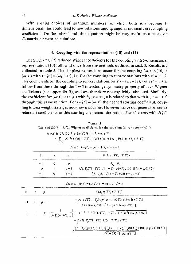
4. Coupling with the representations (10) and (11)

The SO(S) 3 U(2) reduced Wigner coefficients for the coupling with S-dimensional

representation (10) follow at once from the methods outlined in sect. 3. Results are

collected in table 5. The simplest expressions occur for the coupling (w,f) x (10) +

(w{ t’) with (wit’) = (wt + 1 t), i.e. for the coupling to representations with u’ = z’ - 2.

The coefficients for the coupling to representations (w; t’) = {o, - 1 t), with u’ = zi + 2,

follow from these through the 1 c-, 3 interchange symmetry property of such Wigner

coefficients (see appendix B), and are therefore not explicitly tabulated. Similarly,

the coefficient for (w{ t’) = (w, t’) with h,, T = +I, 0 is related to that with h,, T = -1,0

through this same relation. For (w: t’) = (0, t’) the needed starting coefficient, coup-

ling lowest weight states, is not known ab initio. However, since our general formulae

relate all coefficients to this starting coefficient, the ratios of coefficients with H{ T’

TABLE 5

Table of SO(5) 3 U(2) Wigner coefficients for the coupling (w, l) x (10) + (w; I’)

((w,f)H,Ti; (lO)~~~~l(~~~‘)H: = H,i h,T’i’)

=TjFT,; (K ‘(p’(w;r’)T’)),.,‘:(K(p(w,t)T)),,,,F(h,~; rr,,; T’T;)

Casel. (w;t’)=(w,+lr);v’=v-2

h, 7 PI F(h,T; =,,; T’T;,)

-1

0

+1

P 6 6 ?-r TJ,:

P+l U(rT,,7-‘1; rr~,IJlip’;TiT((Po)~,;~lo)I//(P+~,O)~:,)

P+2 4S,,,S,.,,J(p+T,,+3)(p-~,,+2)

Case2. (~it’)=(~,t’); 1’= I*l, t; zr’= 2)

h, = P’ F(h,r; TT;,; T’T;,)

-1 0 P-1 -u(rln;; t’T,l+~(P-l,OtT;; (10)1ll(P0)~~~

(K(l(o,,);‘)),,;[l+(KL(l(w,,)r’)),,l

0 1 p !K(l(~,)r.i),,{(-l,Ti.-l,- ‘U(II?-‘T,,; r’T)J[l+(KZ(l(w,r)r’)),,]

-c U(tT,T’I; ?7‘;)U(t’lT’T;,; t’r;) r,

x (P+l)((PO)T,;(10)1ll(P+~,O)T~~~(POf~~;

J[*+(K’(*(w,r)r’)),,l

ilO)lll(P+LO)q

)

K. T. Hecht / Wigner coejjicients 47

fixed at Hi = --CO: T’= t’ are given, so that the starting coeficient can be evaluated

(to within a phase) from the orthonormality of the Wigner coefficients. For the case

(wit’)=(o,l’) it has the value

c[,,.=((w,I)-w,r; (lO)Ol~~(w,t’)-o,r’)= (K(l(Wt)t’))r,

J[~+(K:“(l(w,tfr’)),,I’ (56)

The specific values for K can be read from eq. (27); for a discussion of the choice

of + sign, see appendix R.

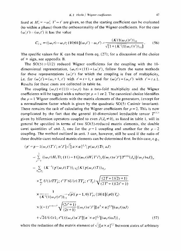
The SO(5) =I U(2) reduced Wigner coefhcients for the coupling with the lo-

dimensional representation, (wr t) x (11) -+ ( OJ{ t’), follow from the same methods

for those representations (~tf’) for which the coupling is free of muitipii~ity,

i.e. for (w~~‘)=(w,*l,~‘) with t’=t*l, t and for (w{t’)=(w,t’) with t’=f+l.

Results for these cases are collected in table 6a.

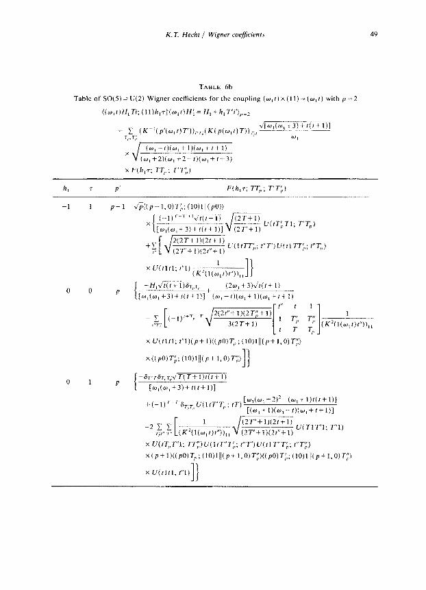
The coupling (w,t) x (11) -$ (w,f) has a two-fold multiplicity and the Wigner

coefficients will be tagged with a subscript p = 1 or 2. The canonical choice identifies

the p = 1 Wigner coefficients with the matrix elements of the generators, (except for

a normalization factor which is given by the quadratic SO(5) Casimir jnvariant~.

There remains the task of calculating the Wigner coefficients for p = 2. This is now

complicated by the fact that the general lo-dimensional irreducible tensor T(“’

given by bifermion operators coupled to even J(Je f 0), as listed in table 1, will in

general be specified in terms of two SO(S)-reduced matrix elements, the double

caret quantities of sect. 3, one for the p = 1 coupling and another for the p = 2

coupling. The method outlined in sect. 3 can, however, still be used if the ratio of

these double-caret reduced matrix elements can be determined first. In this case, e.g.,

(j7’=P-l(w,t)T’i’; ~Y’J’IIJ~[aXa]Jc’llp(~,f)Ti; cd)

= t ((w,t)H,E; (ll)-ll~~(w,t)H~Ir’i’),,~((w,I)~’J’~~T’1”(Je)~~(~lf)~J)),, ,, :- i

= c (K-‘(P’(w,t)7”‘))i’T,:(K(P(w,t)T))_ri,, r,;

where the reduction of the matrix element of &[ a x a]“~’ between states of arbitrary

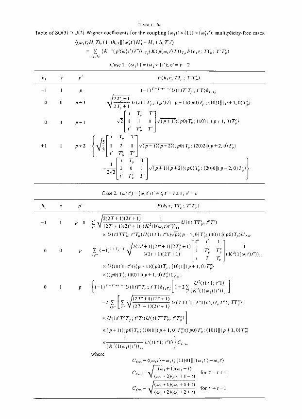
TABLE 621

Table of SO(5) 53 U(2) Wigner coefficients for the coupling (w, 1) x (11) + (w{ I’); multiplicity-free cases.

((w,l)H,Ti; (ll)h,71/(w;t’)H~ = H,+h,T’i’)

= c (K~‘(P’(wll’)T’)),,,,;(K(P(w,l)T)),,,,F(h,7; q,; T’q,) I,,. 1,:

Casel. (o;t’)=(w,+11’);u’=t.-2

h, T P’ F(h,7; 7r, ; r’r;,)

-1 1 P (_l)‘mT’+“G’ U(lrT’q,; I’T)6,,,,

2T’+l 0 0 P+l J &y u(trlr;,; T,,f’)~((PO)T,,;(10)lll(P+l,O)Tb)

P

~((PO)T,,;(10)lll(P+l,O)r~)

--[ 2J3 1 1 f T, 0 T 1 1 J(P+l)(P+2)((PO)~,,;(20)0ll(P+2,O)r;,)

t’ T;, T’

Case2. (w’,t’)=(w,t’)t’#t,I’=t*l;u’=v

h, T P’ F(h,7; 7-q ; T’q,)

x cJ(t17q; r”T,)U(tlt’l; t”l)v$((p-l,O)T;,; (1o)1ll(Po)T,)c,,

1

X(K2(l(w)~“)),, cJ(tlt’l; (“1) c, _

I

where

K. T. Hecht / Wigner coejicients 49

TABLE 6b

Table of SO(5) 2 U(2) Wigner coefficients for the coupling (w, I) x (11) + (w, f) with p = 2

((w,t)H,Ti; (ll)~,~~~(~,r)H~ = H,+ h,T’i’),,=Z

(o,-I)(w,+I)(w,+I+l)

x (w,~2j(w,+2-f)(w,+f+3)

x F(h,q TT;,; T’T;,,

P’ F(h,r; TT,,; T’T;,)

-I 1 p-l \ij;((~-l,~)T:,;(10)1t/(pO))

(.-l)T-T “Ji(G-ij ___ u(tT;,Tl; T’T,)

x{ipO)T;,; (lO)ll/(p+ 1,%-q II 0 1 P

-S~~~S,;,~,:~T(Tfl)t(t+i)

[o,(w, +3)+ f(f+ I)1

+(-1)’ [W,(W,+2)2-(W,+l)t(t+l)l

‘,s,:,,U(lfT’T,,;fT) [(w,+,)(w ,... f)(w,+f+l),

-2 )‘ 7‘ + 7 [

l (~~(l(~,f)f”)),,

~~~ lJ(TlT’1; T”f)

x u(fT,,T”l; n;)u(lrT”T;; t”T’)U(tlT“T;,; r”T;,

X(~+~)((~O)T,,;(~O)~~~(~+~.O)T~)((~O)~;,;(~~)~~~(P+~,O)T~)

x LJ(r1t1; r”1) II

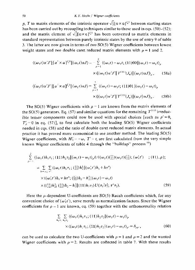
50 K. T. Hecht / Wigner coeficienrs

p, T to matrix elements of the intrinsic operator Ji[a x a]‘~’ between starting states

has been carried out by recoupling techniques similar to those used in eqs. (50)-(52);

and the matrix element of Ji[anxan]‘e’ has been converted to matrix elements in

standard representation between purely intrinsic states by the use of entry 9 of table

3. The latter are now given in terms of two SO(5) Wigner coefficients between lowest

weight states and two double caret reduced matrix elements with p = 1 and 2.

((W,f)U’~‘~~[u+xu]‘~“~~(W,I)LJ)=-~~, ((w,t)--wit; (ll)OO]](w,t)-w,t),

x(((~,t)~‘J’IIT’~“(J,)ll(w,t)aJ)),, (58a)

((W,t)~‘J’ll[a’xa]Jc’ll(w,f)(YJ)= f ((w,t)--w,t; (ll)Olll(w,t)-w,t), p : I

x(((~,fb’J’Il T’“‘(J,)ll(w,t)(~J)), . (58b)

The SO(5) Wigner coefficients with p = 1 are known from the matrix elements of

the SO(5) generators. Eq. (57) and similar equations for the remaining T(“) irreduc-

ible tensor components could now be used with special choices [such as p’= 0,

TL =0 in eq. (57)], to first calculate both the leading SO(5) Wigner coefficients

needed in eqs. (58) and the ratio of double caret reduced matrix elements. In actual

practice it has proved more economical to use another method. The leading SO(5)

Wigner coefficients, with Hi = -w, T’= t, are first calculated from the very simple

known Wigner coefficients of table 4 through the “buildup” process ‘“)

Here the p-dependent U-coefficients are SO(S) Racah coefficients which, for any

convenient choice of (w; t’), serve merely as normalization factors. Since the Wigner

coefficients for p = 1 are known, eq. (59) together with the orthonormality relation

can be used to calculate the two U-coefficients with p = 1 and p = 2 and the wanted

Wigner coefficients with p = 2. Results are collected in table 7. With these results

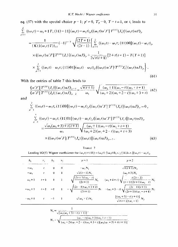
K. T. Hecht / Wigner coejicients

eq. (57) with the special choice p = 1; p’= 0, Tb = 0, T = f f 1, or t, leads to

51

2

c ((w,t)-w,+lT;~ll)-lll~t~,f)--w,~~,~~~~~,~)~’J’II~“‘)(~~l,)ll~~,f)~J)~,~ ,, = I

1

=(K(lfw,t)T)),, (-l)‘-T * d-7 g&y ~~,((o,ri~,r;(ll)oollt~,I)-w,t),,

I

x i ((w,f)-w,C (ll)Olll(~,~)-~,f),,(((w,t)~‘~‘j(T””J;ll(w,l)cuJ)), p - 1

(61) With the entries of table 7 this leads to

((a’J’II T""(J,)(l(w,t)cuJ)),,. , J;cT?i-i ((a~J~II T”“tJ,)ll(w,r)arJ)),,_* =

(w,+l)(~,-o(w,+t+l) (62)

WI (~,+2)(w,+2-t)(w,+3+t)

and

c ((w,f)--w,t; (11)00//t~,~)-~,f),,(~(~,~f~‘J’llT”’~tJ,)ll(~,f)~J~~,, =o, p-l

2

c ((w,t)--w,c (~l)Olll(~,~)-~,~),(((~,~)~‘J’II~~”’(J,)ll(~,~)~J)~,, p=l Jw,(w,+3)+t(t+l) r_=

WI

(63)

TABLE 7

Leading SW51 Wigner coefficients for(~,t)x(1~)~(~,t){(Wlt)h,~,;(lI)hl~Li!(W,t)-~~,t)p

h, TI hz 7, p=l p=2

-01 t 0 0 -wINI JTilTlSNI

-WI f 0 I JFG3N, (0, +3)Nz

-m,+i t-t1 -1 1 ~~~, Co,+d+t) Jo Nz

-w,+1 t-1 -1 I _JTZXN, -iw,+3-.,,J~~r&

-CO,+1 1 -1 1 Y’Cw,+l)N, [(w,+3)-r(r+l)l

Jtcr+l)(w,+l) NL

1 N, =--

xJq(0,+3i+t(t+1)1’ __.-

(co--f)CW,i. I)(w,+r+l)

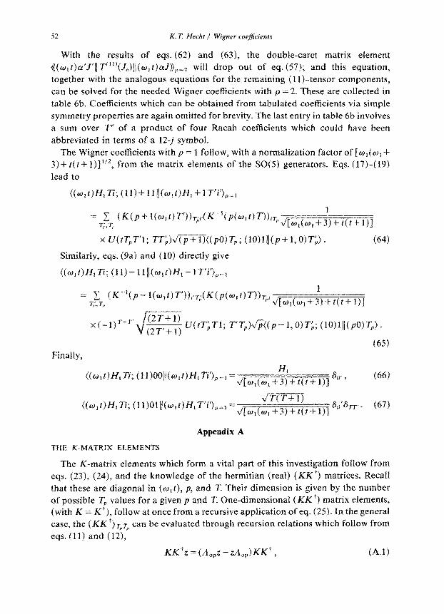
52 K. 7: Hechf / Wigner co@cienrs

With the results of eqs. (62) and (63), the double-caret matrix element

{{(#~~)~‘~‘I1 T”“(~~,)ll(w,t)cYJ)>,, 2 will drop out of eq. (57); and this equation, together with the analogous equations for the remaining (I 1)-tensor components, can be solved for the needed Wigner coefficients with p = 2. These are coliected in table 6b. Coefficients which can be obtained from tabulated coefficients via simple symmetry properties are again omitted for brevity. The last entry in table 6b involves a sum over T” of a product of four Racah coefficients which could have been abbreviated in terms of a 12-j symbol.

The Wigner coefficients with p = 1 follow, with a normalization factor of [cll,(oi + 3)i tit-l- l)]““, from the matrix elements of the SO(5) generators. Eqs. (17)-(19) lead to

‘r,Er (K(P+l(w,f)7"))~:i~(K~~L(P(o*r)T))iT,,~

1

,’ [w,(w,f3)Ct(t+l)-j

Similarly, eqs. (9a) and (10) directly give

~(w~t)H,Ti;(1I)-Il~~(w~t)~,-lT’i’},,,

Finally,

Appendix A

THE K-MATRIX ELEMENTS

The K-matrix elements which form a vital part of this investigation follow from eqs. (23), (24), and the knowledge of the hermitian (real) (KKr) matrices. Recall that these are diagonal in (m,t), p, and T. Their dimension is given by the number of possible T, values for a given p and T. One-dimensional (KK ‘) matrix elements, (with K = K*), follow at once from a recursive application of eq. (25). In the general case, the (XK ‘)?,q, can be evaluated through recursion relations which follow from eqs. (II) and (12),

&X*2 = (/l,,Z - zA,,)KK’ ) (A.11

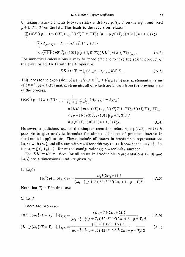
K. T. Hechr / Wigner co.$icients 53

by taking matrix elements between states with fixed JP, T,, T on the right and fixed

p+ 1, TL, T’ on the left. This leads to the recursion relation

;, (KK’(p+l(w,t)T’)),;,,;U(tT,T’I; fl;)m((~O)T,; (lO)lll(~+l,O)~~) P

= $, (4,+, T,:T - 4PT,,T) U( tT,T’1; 7Tb)

xJp+l((pO)?;,;(10)l/I(p+l,O)Tb)(KK’(p(w,t)T)f~~r,,’ (A.2)

For numerical calculations it may be more efficient to take the scalar product of

the z-vector eq. (A.l) with the V operator,

KK~(z~V)=~(n~,,Z,-Z,~4,p)KK~-V;. (A.3) I

This leads to the expression of a single (KK ‘( p + 1 (w, t) T’)) matrix element in terms

of (KK’(p(w,t)T)) matrix elements, al1 of which are known from the previous step

in the process.

x(KK~(p(~~~)T))~,,~;,~(rT~T’l; ~~)~(~~~~I; TT;)

x(P+NWjT,; (W1/l(P+1AT;)

x((pOjT,; (~Oj~ll(P+LOj~b). (A.4)

However, a judicious use of the simpler recursion relation, eq. (A.2), makes it

possible to give analytic formulae for almost all states of practical interest in

shell-model applications. These include all states in irreducible representations

(w, t), with I s :, and all states with p ~4forarbitrary(w,t).Recallthatw,=j+&~v,

(or W, = C (j + f) -Iv for mixed configurations); u = seniority number.

The KK’ = K’ matrices for all states in irreducible representations (w,O) and

(a,$) are l-dimensional and are given by

1. (WIO)

( K2(P(dv T)j77- = 0, !(2w, + l)!!

(w, -$(p+ Tj)!2~‘p-“(2w, + 1 -p+ T)!!

Note that Tp = T in this case.

2. (W,l)

There are two cases

(K*(P(~,~)T= T,+%,,r,,= (CO] -;)!(2w, f2)!!

(WI-;-&?+ T,))!2i(p~f,~‘(20,+2-p+ T,)!!

(K*(p(w,%)7”= T,,-:b,,,,,= (w,-$)!(2qf2)!!

(w,+;-;(p+ T,))!2+~~‘+‘(2w, -p-t T,)!!

(A.51

(A.61

(A.7)

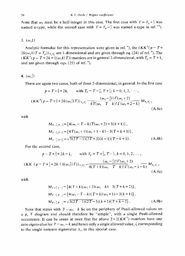
54 K. 7. Hecht / Wigner coeficients

Note that W, must be a half-integer in this case. The first case with T = T, +$ was

named o-type, while the second case with T = T, -4 was named e-type in ref. I’).

3. (Wl)

Analytic formulae for this representation were given in ref. ‘), the (KK.‘( p = T+

2k(w,l)T= Tp))~,,r, are l-dimensional and are given through eq. (24) of ref. “). The

(KK.‘(p = T+2k+ l(w,l) T)) matrices are in general 2-dimensional, with Tp = T* 1,

and are given through eqs. (25) of ref. ‘).

4. (W,$,

There are again two cases, both of them 2-dimensional, in general. In the first case

p = T+$+2k, withT,,=T-$,T+$;k=0,1,2;..,

(KK.‘(p= T+$+2k(w,;)T)&;= (o,-;)!r(w,+2) M

4T(w,-T-k)!T(w,+2-k) ’ T,>T,, 2

(A.8a)

with

MT~;,~-;=[4(~,-T-k)T(~,+2)+3(k+1)1,

MT+;,T+; = [4T(w,+l)(w,+l-k)-3(T+k+l)l,

M,_~,r+;=J3(2T-1)(2T+3)(k+1)(T+k+1). (A.8b)

For the second case,

p = T+;+2k+ 1, with T,, = T-C;, T-i; k=O, 1,2,. . . ,

(w, -$)!l‘(o, +2) (KK’(~=T+:+~~+~(~,~)T))T,.T,:=~(~+~)(,,_~_~)!~(,,+~_~) MT,>T,:,

(A.9a)

with

M,+;,r+; = [4(T+l)(w,+2)(w,-k)-3(T+k+2)],

M,~:,+ = [4(w, -T-k)(T+l)(w,+1)+3(k+l)],

M7+;.T~;=J3(2T-1)(2T+3)(k+1)(T+k+2). (A.9b)

Note that states with T = W, - k lie on the periphery of Pauli-allowed values on

a p, T diagram and should therefore be “simple”, with a single Pauli-allowed

occurrence. It can be seeen at once that the above 2 x2(KKt)-matrices have one

zero eigenvalue for T = w, - k and hence only a single allowed value, i, corresponding

to the single nonzero eigenvalue A,, in this special case.

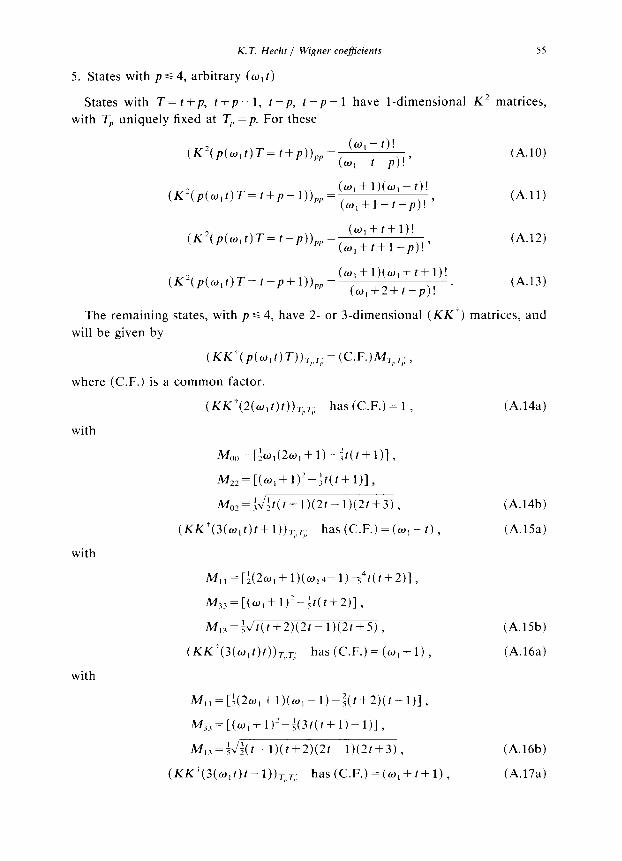
K. T Hecht / Wigner coejicients 55

5. States with p G 4, arbitrary (w, 1)

States with T = t + p, t + p - 1, t -p, t -p - 1 have l-dimensional K2 matrices,

with T, uniquely fixed at T, = p. For these

(w, - t)! (K2(p(W,f)T=f+l)))pp=(W,_I_P)!, (A.lO)

(W,+l)(W,-t)! (K’(P(w)T=~+P-l)),m= (w,+l_t_p)!, (A.ll)

(w,+t+l)! (A.12)

(w, + l)(w, + t + l)! (K’(p(w)T=t-p+l)),,= (w,+2+t_p)! . (A.13)

The remaining states, with p s 4, have 2- or 3-dimensional (KK’) matrices, and

will be given by

(KK’(p(w)T)),,,,,: = (c.F.)W,,,,: ,

where (C.F.) is a common factor.

(KK’(2(w,t)t)),,,,;: has (C.F.) = 1 ,

with

(A.14a)

M,,~=[:w,(2w,+l)-~t(t+l)l,

A&=[(w,+l)‘-$t(t+1)],

M02=:~:I(t+1)(2t-1)(2t+3).

(KKi(3(w,t)t+l))-r,,T,,: has(C.F.)=(w,-t),

(A.14b)

(A.15a)

with

M,,=[:(2w,+l)(w,4-1)~4t(f+2)1,

M,,=[(w,+l)‘-:f(t+2)1,

M,,=~Jr(t+2)(2r-l)(2r+5),

(KK’(3(w,t)t)),,,,,: has(C.F.)=(w,+l),

with

M,,=[:(2w,+l)(w,-l)-:(t+2)(t-l)],

M33=[(W,+1)7-f(3f(t+1)-1)],

M,3=$;(t-l)(t+2)(2t-1)(2t+3),

(KK’(3(wtt)t-l)),,,,,: has(C.F.)=(w,+t+l),

(A.15b)

(A.16a)

(A.16b)

(A.17a)

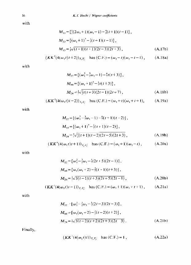
56

with

K. T. Hecht / Wigner coe#iciicients

M,,=[~(2w,+l)(w,-l)-~(r+l)(t-1)],

M33=[(U,+1)2-~(f+l)(r-1)],

M,3=:d(r-l)(t+1)(2r-3)(2r+3), (A.17b)

(f=+(4(~)r+2)),~~; has (C.F.) = (wI - r)(w, -r - 1)) (A.18a)

with

with

M22 = [Cm: -gw,-l)-$r(r+3)],

M.,4=[(~,+1)2-;r(r+3)],

M,,=f&t(t+3)(2r-1)(2r+7), (A.18b)

(KKt(4(W)r-2))T,,T,,: has(C.F.)=(w,+t)(w,+r+l), (A.19a)

Mx= [(m: -3~,-l)-~(r+l)(r-2)],

M44=[(U,+1)2-~(r+l)(r-2)],

M,,=$&(r+l)(r-2)(2r-5)(2r+3), (A.19b)

(KK’(4(w,r)r+l))T,,T,i: has (C.F.) = (w, + l)(w, - r) , (A.20a)

with

with

Finally,

M,,=[wf-;w, -$(2r +5)(2r - I)] ,

M44=[~,(~,+2)-$(r-l)(r+3)],

M,,=+d3(r-l)(r+3)(2r+5)(2r-l), (A.20b)

WKi(4(w,r)r- l)),,,,,: has (C.F.) = (w, + l)(w, + r + 1)) (A.21a)

M22=[~;-$o, -+(2r+3)(2r-3)],

M+,=[~,(~,+2)-$(r-2)(r+2)],

M,,=$/3(r-2)(r+2)(2r+3)(2r-3). (A.21b)

(KK’(4(w,r)r))-,,,-,,: has (C.F.) = 1 , (A.22a)

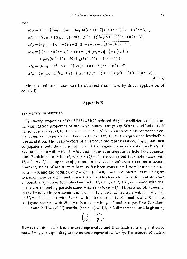
K. T. Hecht / Wigner coejjSm

with

M,,,,={(w,-:)‘o~-f(o, -&~,[4t(t+l)+~]+&t(r+1)(2t-l)(2t+3)},

M,~=[7(2w,+l)(o,-1)-S(r+2)(t-l)]~~~t(t+1)(2?-1)(2~+3),

More complicated cases can be obtained from these by direct application of

eq. (A.4).

Appendix B

SYMMETRY PROPERTIES

Symmetry properties of the SO(5) 13 U(2) reduced Wigner coefficients depend on

the conjugation properties of the SO(S) states. The group SO(5) is self-adjoint. If

the set of matrices, D, for the elements of SO( 5) form an irreducible representation,

the complex conjugates of these matrices, D”, form an equivalent irreducible

representation. The basis vectors of an irreducible representation, (art), and their

conjugates should thus be simply related. Conjugation converts a state with H, , T,

MT into a state with --II], T, -MT and is thus equivalent to particle-hole conjuga-

tion. Particle states with H, s 0, n i (2j+ I), are converted into hole states with

H, b 0, n 3 2j-t 1, upon conjugation. In the vector coherent state construction,

however, states of arbitrary n have so far been constructed from intrinsic states,

with n L= u, and the addition of p = i(n - u)f = 0, T = 1 -coupled pairs reaching up

to a maximum particle number n = 4j + 2 - u. This leads to a very different structure

of possible T, values for hole states with H, 2 0, (n 2 2j + l), compared with that

of the corresponding particle states with H, G 0, (n G 2.i + 1). As a simple example,

in the irreducible representation, (w,t) = (ll), the intrinsic state with n = v, p = 0,

or H, = -I, is a state with T, = 0, with l-dimensional (KK”) matrix and K = 1. Its

conjugate partner, with H, = +I, is a state with p = 2 and two possible T, values,

T, =0 and 2. The (KK’) matrix, (see eq. (A.14)), is 2-dimensional and is given by

However, this matrix has one zero eigenvalue and thus leads to a single allowed

state, i = 1, corresponding to the nonzero eigenvalue, Ai =-$r. The needed K-matrix

58 K. T Hecht / Wigner cwjicienrs

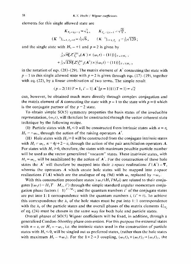
elements for this single allowed state are

K,,,=,.,=, = 4: 2 K,,,,,,,,, =@,

(Km’)i=,,-r,,=“=&&, (K~‘),=,,,,,=*=:,m;

and the single state with H, = +l and p = 2 is given by

~~[z~~~,~(A’)xI(w,t)=(ll))l,=,,, ,

+:i~[Z~~~,(A’)~l(w,r)=(ll))]~=,~, ,

in the notation of eqs. (28)-(29). The matrix element of A’ connecting the state with

p = 1 to this single allowed state with p = 2 is given through eqs. (17)-( 19), together

with eq. (22), by a linear combination of two terms. The simple result

(p=2(11)T= 1, i’= l]lA.‘llp= l(ll)T= l)=&’

can, however, be obtained much more directly through complex conjugation and

the matrix element of A connecting the state with p = 1 to the state with p = 0 which

is the conjugate partner of the p = 2 state.

To obtain simple SO(5) symmetry properties the basis states of the irreducible

representation, (w, t), will therefore be constructed through the vector coherent state

technique by the following recipe.

(I) Particle states with H, s 0 will be constructed from intrinsic states with n = ZI,

H, = --co,, through the action of the raising operators A’.

(II) Hole states with H, a 0 will be constructed from the conjugate intrinsic states

with H, = w,, n = 4j + 2 - u, through the action of the pair annihilation operators A.

For states with H, 2 0, therefore, the states with maximum possible particle number

will be used as the vector generalized “vacuum” states. These instrinsic states, with

H, = w,, will be annihilated by the action of A’. For the construction of these hole

states the A.’ will therefore be mapped into their z-space realizations T(A.‘) = V,

whereas the operators A which create hole states will be mapped into z-space

realizations T(A) which are the analogue of eq. (9d) with w, replaced by -w,.

With this construction procedure states l(w, t) H, TM,i) are related to their conju-

gates I(w,t) - H, T - M,, i”) through the simple standard angular momentum conju-

gation phase factors (- 1) rpM,; and the quantum numbers i” of the conjugate states

are put into 1: 1 correspondence with the quantum numbers i, (i” = i). To achieve

this correspondence the A, of the hole states must be put into 1: 1 correspondence

with the hi of the particle states and the overall phases of the matrix elements Uir,,

of eq. (24) must be chosen in the same way for both hole and particle states.

Overall phases of SO(S) Wigner coefficients will be fixed, in addition, through a

generalized Condon-Shortley phase convention. For this purpose the extremal states

with n = v, or H, = -W , , i.e. the intrinsic states used in the construction of particle

states with H, s 0, will be singled out as preferred states, (rather than the hole states

with maximum H,=+w,). For the 1x2+3 coupling, (w,~),x(w,~)~‘(w,~)~, the

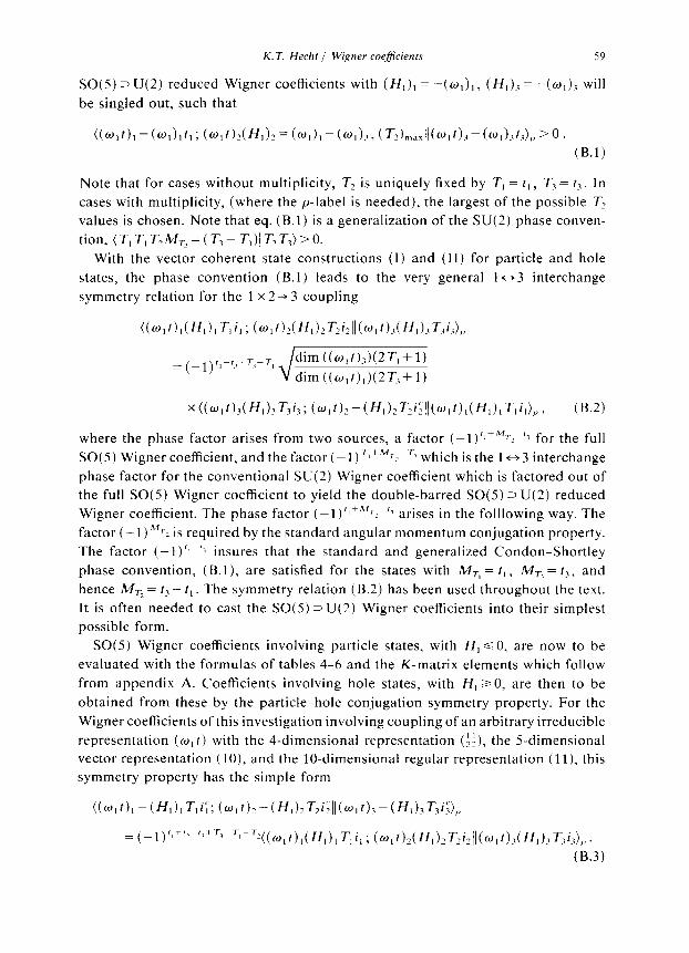
K.T. Hecht / Wiper coej&nts 59

SO(5) 3 U(2) reduced Wigner coefficients with (H,), = -(w,), , (H,)3 = -(w,)? will

be singled out, such that

((w,t),-(@J,),r,; (W,1)2(H,)2=(WI)I-(W,)3. (T,),,,ll(w,r),-(w,),t,),,>O.

(B.1)

Note that for cases without multiplicity, T2 is uniquely fixed by T, = t, , T3 = t,. In

cases with multiplicity, (where the p-label is needed), the largest of the possible T2

values is chosen. Note that eq. (B.1) is a generalization of the SU(2) phase conven-

tion, (T,T,T,M,=(T,-T,)IT,T,)>O. With the vector coherent state constructions (1) and (II) for particle and hole

states, the phase convention (B.l) leads to the very general 1-3 interchange

symmetry relation for the 1 x 2 + 3 coupling

x((W,t)dH,)jT3ij; (W,t)2-(H,),T,i~ll(w,t),(H1),T,i,)p, (B.2)

where the phase factor arises from two sources, a factor (-l)‘~+~‘l~ ‘I for the full

SO(5) Wigner coefficient, and the factor (- 1) T1tMT~m r3 which is the 1 f, 3 interchange

phase factor for the conventional SU(2) Wigner coefficient which is factored out of

the full SO(5) Wigner coefficient to yield the double-barred SO(5) 1 U(2) reduced

Wigner coefficient. The phase factor (-l)‘~+~‘~~~‘~ arises in the folllowing way. The

factor (-1) Ml1 is required by the standard angular momentum conjugation property.

The factor (-l)‘~~‘~ insures that the standard and generalized Condon-Shortley

phase convention, (B.l), are satisfied for the states with M, = t,, M, = t3, and

hence M, = t, - t, . The symmetry relation (B.2) has been used throughout the text.

It is often needed to cast the SO(5) 2 U(2) Wigner coefficients into their simplest

possible form.

SO(5) Wigner coefficients involving particle states, with H, s 0, are now to be

evaluated with the formulas of tables 4-6 and the K-matrix elements which follow

from appendix A. Coefficients involving hole states, with H, ~0, are then to be

obtained from these by the particle-hole conjugation symmetry property. For the

Wigner coefficients of this investigation involving coupling of an arbitrary irreducible

representation (w, t) with the 4-dimensional representation (ii), the 5-dimensional

vector representation (lo), and the lo-dimensional regular representation (1 l), this

symmetry property has the simple form

((Wlt)l-(H1)ITIG; (~,t)~-(H,),T7~~ll(~If)j~(H,)iTji~),,

=(-1) r,+r,-r,+7, I,-r, -((w,t),(H,),T,i,; (WIt)l(HI)2T2i211(WIt)3(Hl)iTii7)l,.

(B.3)

60 K. T. Hecht / Wigner coejicienfs

For couplings involving higher-dimensional irreducible representations (w, t)r with

more complicated multiplicity possibilities, p, additional p-dependent phase factors

may come into play.

The phase conventions of the earlier tabulations of refs. ‘,I’) are unfortunately

dependent on the explicit somewhat more cumbersome state constructions of these

earlier investigations. The results of the present investigation, however, have been

found to agree with the earlier tabulations in all those cases involving only states

with 1 -dimensional (KK ') matrices, with the exception of some overall phase factors.

Certain columns of the earlier Wigner-coefficient unitary transformation matrices

have to be multiplied by factors of (-1) to bring them into agreement with the

results of tables 4-6. Once the overall phase has been established, through the

evaluation of a simple special case, e.g., the earlier tabulations can be used in

conjunction with the present results.

References

1) D.J. Rowe, J. Math. Phys. 25 (1984) 2662

2) D.J. Rowe, G. Rosensteel and R. Gihnore, J. Math. Phys. 26 (1985) 2787

3) J. Deenen and C. Quesne, J. Math. Phys. 25 (1984) 1638, 2354

4) C. Quesne, J. Math. Phys. 27 (1986) 428, 869

5) D.J. Rowe, R. Le Blanc and K.T. Hecht, J. Math. Phys. 29 (1988) 287

6) K.T. Hecht, The vector coherent state method and its application to problems of higher symmetries,

Lecture Notes in Physics 290 (Springer, Berlin, 1987). 7) R. Le Blanc and K.T. Hecht, J. of Phys. A20 (1987) 4613 8) R. Le Blanc and L.C. Biedenharn, J. of Phys. A22 (1989) 31

9) K.T. Hecht and J.P. Elliott, Nucl. Phys. A438 (1985) 29

10) K.T. Hecht, Nucl. Phys. Al02 (1967) 11; and references therein

11) R.P. Hemenger and K.T. Hecht, Nucl. Phys. Al45 (1970) 468; and references therein