Embed Size (px)
Citation preview

WIEN2kAn Augmented Plane Wave Plus Local Orbitals Program
for Calculating Crystal Properties
User’s Guide, September 18, 2008
Peter BlahaKarlheinz Schwarz
Georg MadsenDieter Kvasnicka
Joachim Luitz
Vienna University of TechnologyInst. of Physical and Theoretical Chemistry
Getreidemarkt 9/156, A-1060 Vienna/Austria

Peter Blaha, Karlheinz Schwarz, Georg K. H. Madsen, Dieter Kvasnicka, Joachim Luitz:WIEN2kAn Augmented Plane Wave + Local Orbitals Program for Calculating Crystal Properties
revised edition WIEN2k 08.3 (Release 18/9/2008)
Univ. Prof. Dr. Karlheinz SchwarzTechn. Universitat WienInstitut fur Physikalische und Theoretische ChemieGetreidemarkt 9/156A-1060 Wien/AustriaISBN 3-9501031-1-2
ISBN 3-9501031-1-2

Contents
1 Introduction 1
I Introduction to the WIEN2k package 5
2 Basic concepts 7
2.1 Density Functional Theory . . . . . . . . . . . . . . . . . . . . . . . . . . . . . . . . . . 7
2.2 The APW Methods . . . . . . . . . . . . . . . . . . . . . . . . . . . . . . . . . . . . . . 8
2.2.1 The LAPW Method . . . . . . . . . . . . . . . . . . . . . . . . . . . . . . . . . . 8
2.2.2 The APW+lo Method . . . . . . . . . . . . . . . . . . . . . . . . . . . . . . . . . 9
2.2.3 General considerations . . . . . . . . . . . . . . . . . . . . . . . . . . . . . . . . 10
3 Quick Start 13
3.1 Naming conventions . . . . . . . . . . . . . . . . . . . . . . . . . . . . . . . . . . . . . 13
3.2 Starting the server . . . . . . . . . . . . . . . . . . . . . . . . . . . . . . . . . . . . . . . 14
3.3 Connecting to the w2web server . . . . . . . . . . . . . . . . . . . . . . . . . . . . . . 15
3.4 Creating a new session . . . . . . . . . . . . . . . . . . . . . . . . . . . . . . . . . . . . 15
3.5 Creating a new case . . . . . . . . . . . . . . . . . . . . . . . . . . . . . . . . . . . . . . 16
3.6 Creating the struct file . . . . . . . . . . . . . . . . . . . . . . . . . . . . . . . . . . . . 16
3.7 Initialization . . . . . . . . . . . . . . . . . . . . . . . . . . . . . . . . . . . . . . . . . . 18
3.8 The SCF calculation . . . . . . . . . . . . . . . . . . . . . . . . . . . . . . . . . . . . . . 20
3.9 The case.scf file . . . . . . . . . . . . . . . . . . . . . . . . . . . . . . . . . . . . . . . . 21
3.10 Saving a calculation . . . . . . . . . . . . . . . . . . . . . . . . . . . . . . . . . . . . . . 21
3.11 Calculating properties . . . . . . . . . . . . . . . . . . . . . . . . . . . . . . . . . . . . 21
3.11.1 Electron density plots . . . . . . . . . . . . . . . . . . . . . . . . . . . . . . . . 21
3.11.2 Density of States (DOS) . . . . . . . . . . . . . . . . . . . . . . . . . . . . . . . 24
3.11.3 X-ray spectra . . . . . . . . . . . . . . . . . . . . . . . . . . . . . . . . . . . . . 26
3.11.4 Bandstructure . . . . . . . . . . . . . . . . . . . . . . . . . . . . . . . . . . . . . 26
3.11.5 Bandstructure with band character plotting / full lines . . . . . . . . . . . . . 27
3.11.6 Volume Optimization . . . . . . . . . . . . . . . . . . . . . . . . . . . . . . . . 28
3.12 Setting up a new case . . . . . . . . . . . . . . . . . . . . . . . . . . . . . . . . . . . . . 29
3.12.1 Manual setup . . . . . . . . . . . . . . . . . . . . . . . . . . . . . . . . . . . . . 29
3.12.2 Setting up a new case using w2web . . . . . . . . . . . . . . . . . . . . . . . . 29
3

II Detailed description of the files and programs of the WIEN2k package 31
4 Files and Program Flow 33
4.1 Flow of input and output files . . . . . . . . . . . . . . . . . . . . . . . . . . . . . . . . 33
4.2 Input/Output files . . . . . . . . . . . . . . . . . . . . . . . . . . . . . . . . . . . . . . 37
4.3 The case.struct.file . . . . . . . . . . . . . . . . . . . . . . . . . . . . . . . . . . . . . . . 38
4.4 The case.scf file . . . . . . . . . . . . . . . . . . . . . . . . . . . . . . . . . . . . . . . . 41
4.5 Flow of programs . . . . . . . . . . . . . . . . . . . . . . . . . . . . . . . . . . . . . . . 43
4.5.1 Core, semi-core and valence states . . . . . . . . . . . . . . . . . . . . . . . . . 43
4.5.2 Spin-polarized calculation . . . . . . . . . . . . . . . . . . . . . . . . . . . . . . 45
4.5.3 Fixed-spin-moment (FSM) calculations . . . . . . . . . . . . . . . . . . . . . . 45
4.5.4 Antiferromagnetic (AFM) calculations . . . . . . . . . . . . . . . . . . . . . . . 45
4.5.5 Spin-orbit interaction . . . . . . . . . . . . . . . . . . . . . . . . . . . . . . . . . 46
4.5.6 Orbital potentials . . . . . . . . . . . . . . . . . . . . . . . . . . . . . . . . . . . 47
4.5.7 Exact-exchange and Hybrid functionals for correlated electrons . . . . . . . . 47
5 Shell scripts 51
5.1 Job control . . . . . . . . . . . . . . . . . . . . . . . . . . . . . . . . . . . . . . . . . . . 51
5.1.1 Main execution script (x lapw) . . . . . . . . . . . . . . . . . . . . . . . . . . . 51
5.1.2 Job control for initialization (init lapw) . . . . . . . . . . . . . . . . . . . . . . 52
5.1.3 Job control for iteration (run lapw or runsp lapw) . . . . . . . . . . . . . . . . 52
5.2 Utility scripts . . . . . . . . . . . . . . . . . . . . . . . . . . . . . . . . . . . . . . . . . 54
5.2.1 Save a calculation (save lapw) . . . . . . . . . . . . . . . . . . . . . . . . . . . 54
5.2.2 Restoring a calculation (restore lapw) . . . . . . . . . . . . . . . . . . . . . . . 55
5.2.3 Remove unnecessary files (clean lapw) . . . . . . . . . . . . . . . . . . . . . . 55
5.2.4 Migrate a case to/from a remote computer (migrate lapw) . . . . . . . . . . . 55
5.2.5 Generate case.inst (instgen lapw) . . . . . . . . . . . . . . . . . . . . . . . . . . 56
5.2.6 Set R-MT values in your case.struct file (setrmt lapw) . . . . . . . . . . . . . . 56
5.2.7 Check for running WIEN jobs (check lapw) . . . . . . . . . . . . . . . . . . . . 56
5.2.8 Cancel (kill) running WIEN jobs (cancel lapw) . . . . . . . . . . . . . . . . . . 56
5.2.9 Extract critical points from a Bader analysis (extractaim lapw) . . . . . . . . . 56
5.2.10 scfmonitor lapw . . . . . . . . . . . . . . . . . . . . . . . . . . . . . . . . . . . 57
5.2.11 analyse lapw . . . . . . . . . . . . . . . . . . . . . . . . . . . . . . . . . . . . . 57
5.2.12 Check parallel execution (testpara lapw) . . . . . . . . . . . . . . . . . . . . . 58
5.2.13 Check parallel execution of lapw1 (testpara1 lapw) . . . . . . . . . . . . . . . 58
5.2.14 Check parallel execution of lapw2 (testpara2 lapw) . . . . . . . . . . . . . . . 58
5.2.15 grepline lapw . . . . . . . . . . . . . . . . . . . . . . . . . . . . . . . . . . . . . 58
5.2.16 initso lapw . . . . . . . . . . . . . . . . . . . . . . . . . . . . . . . . . . . . . . 58
5.2.17 vec2old lapw . . . . . . . . . . . . . . . . . . . . . . . . . . . . . . . . . . . . . 59
5.2.18 clmextrapol lapw . . . . . . . . . . . . . . . . . . . . . . . . . . . . . . . . . . . 59
5.3 Structure optimization . . . . . . . . . . . . . . . . . . . . . . . . . . . . . . . . . . . . 59
5.3.1 Lattice parameters (Volume, c/a, lattice parameters) . . . . . . . . . . . . . . . 59
5.3.2 Minimization of internal parameters (min lapw) . . . . . . . . . . . . . . . . . 60
5.4 Phonon calculations . . . . . . . . . . . . . . . . . . . . . . . . . . . . . . . . . . . . . . 63
5.4.1 init phonon lapw . . . . . . . . . . . . . . . . . . . . . . . . . . . . . . . . . . . 63
5.4.2 analyse phonon lapw . . . . . . . . . . . . . . . . . . . . . . . . . . . . . . . . 63
5.5 Parallel Execution . . . . . . . . . . . . . . . . . . . . . . . . . . . . . . . . . . . . . . . 63
5.5.1 k-Point Parallelization . . . . . . . . . . . . . . . . . . . . . . . . . . . . . . . . 64
5.5.2 MPI parallelization . . . . . . . . . . . . . . . . . . . . . . . . . . . . . . . . . . 64
5.5.3 How to use WIEN2k as a parallel program . . . . . . . . . . . . . . . . . . . . 64
5.5.4 The .machines file . . . . . . . . . . . . . . . . . . . . . . . . . . . . . . . . . 65
5.5.5 How the list of k-points is split . . . . . . . . . . . . . . . . . . . . . . . . . . . 66
5.5.6 Flow chart of the parallel scripts . . . . . . . . . . . . . . . . . . . . . . . . . . 67
5.5.7 On the fine grained parallelization . . . . . . . . . . . . . . . . . . . . . . . . . 67
5.6 Getting on-line help . . . . . . . . . . . . . . . . . . . . . . . . . . . . . . . . . . . . . . 69
5.7 Interface scripts . . . . . . . . . . . . . . . . . . . . . . . . . . . . . . . . . . . . . . . . 69
5.7.1 eplot lapw . . . . . . . . . . . . . . . . . . . . . . . . . . . . . . . . . . . . . . . 69
5.7.2 parabolfit lapw . . . . . . . . . . . . . . . . . . . . . . . . . . . . . . . . . . . . 70
5.7.3 dosplot lapw . . . . . . . . . . . . . . . . . . . . . . . . . . . . . . . . . . . . . 70
5.7.4 dosplot2 lapw . . . . . . . . . . . . . . . . . . . . . . . . . . . . . . . . . . . . . 70
5.7.5 Curve lapw . . . . . . . . . . . . . . . . . . . . . . . . . . . . . . . . . . . . . . 70
5.7.6 specplot lapw . . . . . . . . . . . . . . . . . . . . . . . . . . . . . . . . . . . . . 70
5.7.7 rhoplot lapw . . . . . . . . . . . . . . . . . . . . . . . . . . . . . . . . . . . . . 70
5.7.8 opticplot lapw . . . . . . . . . . . . . . . . . . . . . . . . . . . . . . . . . . . . 71
5.7.9 addjoint-updn lapw . . . . . . . . . . . . . . . . . . . . . . . . . . . . . . . . . 71
6 Initialization 73
6.1 NN . . . . . . . . . . . . . . . . . . . . . . . . . . . . . . . . . . . . . . . . . . . . . . . 73
6.1.1 Execution . . . . . . . . . . . . . . . . . . . . . . . . . . . . . . . . . . . . . . . 73
6.2 SGROUP . . . . . . . . . . . . . . . . . . . . . . . . . . . . . . . . . . . . . . . . . . . . 74
6.2.1 Execution . . . . . . . . . . . . . . . . . . . . . . . . . . . . . . . . . . . . . . . 74
6.3 SYMMETRY . . . . . . . . . . . . . . . . . . . . . . . . . . . . . . . . . . . . . . . . . . 74
6.3.1 Execution . . . . . . . . . . . . . . . . . . . . . . . . . . . . . . . . . . . . . . . 74
6.4 LSTART . . . . . . . . . . . . . . . . . . . . . . . . . . . . . . . . . . . . . . . . . . . . . 75
6.4.1 Execution . . . . . . . . . . . . . . . . . . . . . . . . . . . . . . . . . . . . . . . 75
6.4.2 Dimensioning parameters . . . . . . . . . . . . . . . . . . . . . . . . . . . . . . 75
6.4.3 Input . . . . . . . . . . . . . . . . . . . . . . . . . . . . . . . . . . . . . . . . . . 75
6.5 KGEN . . . . . . . . . . . . . . . . . . . . . . . . . . . . . . . . . . . . . . . . . . . . . . 77

6.5.1 Execution . . . . . . . . . . . . . . . . . . . . . . . . . . . . . . . . . . . . . . . 77
6.5.2 Dimensioning parameters . . . . . . . . . . . . . . . . . . . . . . . . . . . . . . 78
6.6 DSTART . . . . . . . . . . . . . . . . . . . . . . . . . . . . . . . . . . . . . . . . . . . . 78
6.6.1 Execution . . . . . . . . . . . . . . . . . . . . . . . . . . . . . . . . . . . . . . . 78
6.6.2 Dimensioning parameters . . . . . . . . . . . . . . . . . . . . . . . . . . . . . . 78
7 SCF cycle 79
7.1 LAPW0 . . . . . . . . . . . . . . . . . . . . . . . . . . . . . . . . . . . . . . . . . . . . . 79
7.1.1 Execution . . . . . . . . . . . . . . . . . . . . . . . . . . . . . . . . . . . . . . . 80
7.1.2 Dimensioning parameters . . . . . . . . . . . . . . . . . . . . . . . . . . . . . . 80
7.1.3 Input . . . . . . . . . . . . . . . . . . . . . . . . . . . . . . . . . . . . . . . . . . 80
7.2 ORB . . . . . . . . . . . . . . . . . . . . . . . . . . . . . . . . . . . . . . . . . . . . . . . 82
7.2.1 Execution . . . . . . . . . . . . . . . . . . . . . . . . . . . . . . . . . . . . . . . 83
7.2.2 Dimensioning parameters . . . . . . . . . . . . . . . . . . . . . . . . . . . . . . 83
7.2.3 Input . . . . . . . . . . . . . . . . . . . . . . . . . . . . . . . . . . . . . . . . . . 83
7.3 LAPW1 . . . . . . . . . . . . . . . . . . . . . . . . . . . . . . . . . . . . . . . . . . . . . 86
7.3.1 Execution . . . . . . . . . . . . . . . . . . . . . . . . . . . . . . . . . . . . . . . 86
7.3.2 Dimensioning parameters . . . . . . . . . . . . . . . . . . . . . . . . . . . . . . 86
7.3.3 Input . . . . . . . . . . . . . . . . . . . . . . . . . . . . . . . . . . . . . . . . . . 87
7.4 LAPWSO . . . . . . . . . . . . . . . . . . . . . . . . . . . . . . . . . . . . . . . . . . . . 91
7.4.1 Execution . . . . . . . . . . . . . . . . . . . . . . . . . . . . . . . . . . . . . . . 91
7.4.2 Dimensioning parameters . . . . . . . . . . . . . . . . . . . . . . . . . . . . . . 91
7.4.3 Input . . . . . . . . . . . . . . . . . . . . . . . . . . . . . . . . . . . . . . . . . . 92
7.5 LAPW2 . . . . . . . . . . . . . . . . . . . . . . . . . . . . . . . . . . . . . . . . . . . . . 93
7.5.1 Execution . . . . . . . . . . . . . . . . . . . . . . . . . . . . . . . . . . . . . . . 93
7.5.2 Dimensioning parameters . . . . . . . . . . . . . . . . . . . . . . . . . . . . . . 93
7.5.3 Input . . . . . . . . . . . . . . . . . . . . . . . . . . . . . . . . . . . . . . . . . . 94
7.6 SUMPARA . . . . . . . . . . . . . . . . . . . . . . . . . . . . . . . . . . . . . . . . . . . 97
7.6.1 Execution . . . . . . . . . . . . . . . . . . . . . . . . . . . . . . . . . . . . . . . 97
7.6.2 Dimensioning parameters . . . . . . . . . . . . . . . . . . . . . . . . . . . . . . 97
7.7 LAPWDM . . . . . . . . . . . . . . . . . . . . . . . . . . . . . . . . . . . . . . . . . . . 98
7.7.1 Execution . . . . . . . . . . . . . . . . . . . . . . . . . . . . . . . . . . . . . . . 98
7.7.2 Dimensioning parameters . . . . . . . . . . . . . . . . . . . . . . . . . . . . . . 98
7.7.3 Input . . . . . . . . . . . . . . . . . . . . . . . . . . . . . . . . . . . . . . . . . . 99
7.8 LCORE . . . . . . . . . . . . . . . . . . . . . . . . . . . . . . . . . . . . . . . . . . . . . 99
7.8.1 Execution . . . . . . . . . . . . . . . . . . . . . . . . . . . . . . . . . . . . . . . 99
7.8.2 Dimensioning parameters . . . . . . . . . . . . . . . . . . . . . . . . . . . . . . 100
7.8.3 Input . . . . . . . . . . . . . . . . . . . . . . . . . . . . . . . . . . . . . . . . . . 100
7.9 MIXER . . . . . . . . . . . . . . . . . . . . . . . . . . . . . . . . . . . . . . . . . . . . . 101

7.9.1 Execution . . . . . . . . . . . . . . . . . . . . . . . . . . . . . . . . . . . . . . . 101
7.9.2 Dimensioning parameters . . . . . . . . . . . . . . . . . . . . . . . . . . . . . . 101
7.9.3 Input . . . . . . . . . . . . . . . . . . . . . . . . . . . . . . . . . . . . . . . . . . 102
8 Analysis, Properties and Optimization 105
8.1 TETRA . . . . . . . . . . . . . . . . . . . . . . . . . . . . . . . . . . . . . . . . . . . . . 105
8.1.1 Execution . . . . . . . . . . . . . . . . . . . . . . . . . . . . . . . . . . . . . . . 106
8.1.2 Dimensioning parameters . . . . . . . . . . . . . . . . . . . . . . . . . . . . . . 106
8.1.3 Input . . . . . . . . . . . . . . . . . . . . . . . . . . . . . . . . . . . . . . . . . . 106
8.2 QTL . . . . . . . . . . . . . . . . . . . . . . . . . . . . . . . . . . . . . . . . . . . . . . . 107
8.2.1 Execution . . . . . . . . . . . . . . . . . . . . . . . . . . . . . . . . . . . . . . . 108
8.2.2 Input . . . . . . . . . . . . . . . . . . . . . . . . . . . . . . . . . . . . . . . . . . 108
8.2.3 Output . . . . . . . . . . . . . . . . . . . . . . . . . . . . . . . . . . . . . . . . . 109
8.3 SPAGHETTI . . . . . . . . . . . . . . . . . . . . . . . . . . . . . . . . . . . . . . . . . . 110
8.3.1 Execution . . . . . . . . . . . . . . . . . . . . . . . . . . . . . . . . . . . . . . . 110
8.3.2 Input . . . . . . . . . . . . . . . . . . . . . . . . . . . . . . . . . . . . . . . . . . 110
8.4 IRREP . . . . . . . . . . . . . . . . . . . . . . . . . . . . . . . . . . . . . . . . . . . . . . 112
8.4.1 Execution . . . . . . . . . . . . . . . . . . . . . . . . . . . . . . . . . . . . . . . 113
8.4.2 Dimensioning parameters . . . . . . . . . . . . . . . . . . . . . . . . . . . . . . 113
8.5 LAPW3 . . . . . . . . . . . . . . . . . . . . . . . . . . . . . . . . . . . . . . . . . . . . . 113
8.5.1 Execution . . . . . . . . . . . . . . . . . . . . . . . . . . . . . . . . . . . . . . . 114
8.5.2 Dimensioning parameters . . . . . . . . . . . . . . . . . . . . . . . . . . . . . . 114
8.6 LAPW5 . . . . . . . . . . . . . . . . . . . . . . . . . . . . . . . . . . . . . . . . . . . . . 114
8.6.1 Execution . . . . . . . . . . . . . . . . . . . . . . . . . . . . . . . . . . . . . . . 114
8.6.2 Dimensioning parameters . . . . . . . . . . . . . . . . . . . . . . . . . . . . . . 114
8.6.3 Input . . . . . . . . . . . . . . . . . . . . . . . . . . . . . . . . . . . . . . . . . . 115
8.7 AIM . . . . . . . . . . . . . . . . . . . . . . . . . . . . . . . . . . . . . . . . . . . . . . . 116
8.7.1 Execution . . . . . . . . . . . . . . . . . . . . . . . . . . . . . . . . . . . . . . . 117
8.7.2 Dimensioning parameters . . . . . . . . . . . . . . . . . . . . . . . . . . . . . . 117
8.7.3 Input . . . . . . . . . . . . . . . . . . . . . . . . . . . . . . . . . . . . . . . . . . 117
8.8 LAPW7 . . . . . . . . . . . . . . . . . . . . . . . . . . . . . . . . . . . . . . . . . . . . . 120
8.8.1 Execution . . . . . . . . . . . . . . . . . . . . . . . . . . . . . . . . . . . . . . . 120
8.8.2 Dimensioning parameters . . . . . . . . . . . . . . . . . . . . . . . . . . . . . . 121
8.8.3 Input . . . . . . . . . . . . . . . . . . . . . . . . . . . . . . . . . . . . . . . . . . 121
8.9 FILTVEC . . . . . . . . . . . . . . . . . . . . . . . . . . . . . . . . . . . . . . . . . . . . 124
8.9.1 Execution . . . . . . . . . . . . . . . . . . . . . . . . . . . . . . . . . . . . . . . 124
8.9.2 Dimensioning parameters . . . . . . . . . . . . . . . . . . . . . . . . . . . . . . 124
8.9.3 Input . . . . . . . . . . . . . . . . . . . . . . . . . . . . . . . . . . . . . . . . . . 125
8.10 XSPEC . . . . . . . . . . . . . . . . . . . . . . . . . . . . . . . . . . . . . . . . . . . . . 126

8.10.1 Execution . . . . . . . . . . . . . . . . . . . . . . . . . . . . . . . . . . . . . . . 126
8.10.2 Dimensioning parameters . . . . . . . . . . . . . . . . . . . . . . . . . . . . . . 127
8.10.3 Input . . . . . . . . . . . . . . . . . . . . . . . . . . . . . . . . . . . . . . . . . . 127
8.11 TELNES.2 . . . . . . . . . . . . . . . . . . . . . . . . . . . . . . . . . . . . . . . . . . . 129
8.11.1 Execution . . . . . . . . . . . . . . . . . . . . . . . . . . . . . . . . . . . . . . . 130
8.11.2 Input . . . . . . . . . . . . . . . . . . . . . . . . . . . . . . . . . . . . . . . . . . 130
8.12 BROADENING . . . . . . . . . . . . . . . . . . . . . . . . . . . . . . . . . . . . . . . . 134
8.12.1 Execution . . . . . . . . . . . . . . . . . . . . . . . . . . . . . . . . . . . . . . . 134
8.12.2 Input . . . . . . . . . . . . . . . . . . . . . . . . . . . . . . . . . . . . . . . . . . 134
8.13 OPTIMIZE . . . . . . . . . . . . . . . . . . . . . . . . . . . . . . . . . . . . . . . . . . . 135
8.13.1 Execution . . . . . . . . . . . . . . . . . . . . . . . . . . . . . . . . . . . . . . . 135
8.13.2 Input . . . . . . . . . . . . . . . . . . . . . . . . . . . . . . . . . . . . . . . . . . 135
8.14 ELAST . . . . . . . . . . . . . . . . . . . . . . . . . . . . . . . . . . . . . . . . . . . . . 135
8.14.1 Execution . . . . . . . . . . . . . . . . . . . . . . . . . . . . . . . . . . . . . . . 136
8.15 MINI . . . . . . . . . . . . . . . . . . . . . . . . . . . . . . . . . . . . . . . . . . . . . . 136
8.15.1 Execution . . . . . . . . . . . . . . . . . . . . . . . . . . . . . . . . . . . . . . . 137
8.15.2 Dimensioning parameters . . . . . . . . . . . . . . . . . . . . . . . . . . . . . . 137
8.15.3 Input . . . . . . . . . . . . . . . . . . . . . . . . . . . . . . . . . . . . . . . . . . 137
8.16 OPTIC . . . . . . . . . . . . . . . . . . . . . . . . . . . . . . . . . . . . . . . . . . . . . 139
8.16.1 Execution . . . . . . . . . . . . . . . . . . . . . . . . . . . . . . . . . . . . . . . 139
8.16.2 Dimensioning parameters . . . . . . . . . . . . . . . . . . . . . . . . . . . . . . 140
8.16.3 Input . . . . . . . . . . . . . . . . . . . . . . . . . . . . . . . . . . . . . . . . . . 140
8.17 JOINT . . . . . . . . . . . . . . . . . . . . . . . . . . . . . . . . . . . . . . . . . . . . . . 142
8.17.1 Execution . . . . . . . . . . . . . . . . . . . . . . . . . . . . . . . . . . . . . . . 142
8.17.2 Dimensioning parameters . . . . . . . . . . . . . . . . . . . . . . . . . . . . . . 142
8.17.3 Input . . . . . . . . . . . . . . . . . . . . . . . . . . . . . . . . . . . . . . . . . . 142
8.18 KRAM . . . . . . . . . . . . . . . . . . . . . . . . . . . . . . . . . . . . . . . . . . . . . 143
8.18.1 Execution . . . . . . . . . . . . . . . . . . . . . . . . . . . . . . . . . . . . . . . 144
8.18.2 Dimensioning parameters . . . . . . . . . . . . . . . . . . . . . . . . . . . . . . 144
8.18.3 Input . . . . . . . . . . . . . . . . . . . . . . . . . . . . . . . . . . . . . . . . . . 144
8.19 FSGEN . . . . . . . . . . . . . . . . . . . . . . . . . . . . . . . . . . . . . . . . . . . . . 145
9 Utility Programs 147
9.1 symmetso . . . . . . . . . . . . . . . . . . . . . . . . . . . . . . . . . . . . . . . . . . . 147
9.1.1 Execution . . . . . . . . . . . . . . . . . . . . . . . . . . . . . . . . . . . . . . . 148
9.2 pairhess . . . . . . . . . . . . . . . . . . . . . . . . . . . . . . . . . . . . . . . . . . . . . 148
9.2.1 Execution . . . . . . . . . . . . . . . . . . . . . . . . . . . . . . . . . . . . . . . 148
9.2.2 Dimensioning parameters . . . . . . . . . . . . . . . . . . . . . . . . . . . . . . 148
9.2.3 Input . . . . . . . . . . . . . . . . . . . . . . . . . . . . . . . . . . . . . . . . . . 149

9.3 afminput . . . . . . . . . . . . . . . . . . . . . . . . . . . . . . . . . . . . . . . . . . . . 149
9.3.1 Execution . . . . . . . . . . . . . . . . . . . . . . . . . . . . . . . . . . . . . . . 150
9.3.2 Dimensioning parameters . . . . . . . . . . . . . . . . . . . . . . . . . . . . . . 150
9.4 clmcopy . . . . . . . . . . . . . . . . . . . . . . . . . . . . . . . . . . . . . . . . . . . . 150
9.4.1 Execution . . . . . . . . . . . . . . . . . . . . . . . . . . . . . . . . . . . . . . . 150
9.4.2 Dimensioning parameters . . . . . . . . . . . . . . . . . . . . . . . . . . . . . . 150
9.4.3 Input . . . . . . . . . . . . . . . . . . . . . . . . . . . . . . . . . . . . . . . . . . 151
9.5 reformat . . . . . . . . . . . . . . . . . . . . . . . . . . . . . . . . . . . . . . . . . . . . 152
9.6 hex2rhomb and rhomb in5 . . . . . . . . . . . . . . . . . . . . . . . . . . . . . . . . . . 152
9.7 plane . . . . . . . . . . . . . . . . . . . . . . . . . . . . . . . . . . . . . . . . . . . . . . 152
9.8 add columns . . . . . . . . . . . . . . . . . . . . . . . . . . . . . . . . . . . . . . . . . . 152
9.9 clminter . . . . . . . . . . . . . . . . . . . . . . . . . . . . . . . . . . . . . . . . . . . . . 152
9.10 eosfit . . . . . . . . . . . . . . . . . . . . . . . . . . . . . . . . . . . . . . . . . . . . . . 153
9.11 eosfit6 . . . . . . . . . . . . . . . . . . . . . . . . . . . . . . . . . . . . . . . . . . . . . . 153
9.12 spacegroup . . . . . . . . . . . . . . . . . . . . . . . . . . . . . . . . . . . . . . . . . . . 153
9.13 xyz2struct . . . . . . . . . . . . . . . . . . . . . . . . . . . . . . . . . . . . . . . . . . . 154
9.14 cif2struct . . . . . . . . . . . . . . . . . . . . . . . . . . . . . . . . . . . . . . . . . . . . 154
9.15 struct2cif . . . . . . . . . . . . . . . . . . . . . . . . . . . . . . . . . . . . . . . . . . . . 154
9.16 StructGen of w2web . . . . . . . . . . . . . . . . . . . . . . . . . . . . . . . . . . . . . 155
9.17 supercell . . . . . . . . . . . . . . . . . . . . . . . . . . . . . . . . . . . . . . . . . . . . 155
9.17.1 Execution . . . . . . . . . . . . . . . . . . . . . . . . . . . . . . . . . . . . . . . 155
9.18 structeditor . . . . . . . . . . . . . . . . . . . . . . . . . . . . . . . . . . . . . . . . . . . 155
9.18.1 Execution . . . . . . . . . . . . . . . . . . . . . . . . . . . . . . . . . . . . . . . 156
9.19 Visualization . . . . . . . . . . . . . . . . . . . . . . . . . . . . . . . . . . . . . . . . . . 157
9.19.1 BALSAC . . . . . . . . . . . . . . . . . . . . . . . . . . . . . . . . . . . . . . . . 157
9.19.2 XCrysDen . . . . . . . . . . . . . . . . . . . . . . . . . . . . . . . . . . . . . . . 157
10 Examples 159
10.1 TiC . . . . . . . . . . . . . . . . . . . . . . . . . . . . . . . . . . . . . . . . . . . . . . . 159
10.2 FCC Nickel . . . . . . . . . . . . . . . . . . . . . . . . . . . . . . . . . . . . . . . . . . . 159
10.3 Rutile . . . . . . . . . . . . . . . . . . . . . . . . . . . . . . . . . . . . . . . . . . . . . . 160
10.4 supercell calc . . . . . . . . . . . . . . . . . . . . . . . . . . . . . . . . . . . . . . . . . . 161
III Installation of the WIEN2k package and Dimensioning of programs 163
11 Installation and Dimensioning 165
11.1 Requirements . . . . . . . . . . . . . . . . . . . . . . . . . . . . . . . . . . . . . . . . . 165
11.2 Installation of WIEN2k . . . . . . . . . . . . . . . . . . . . . . . . . . . . . . . . . . . . 166
11.2.1 Expanding the WIEN2k distribution . . . . . . . . . . . . . . . . . . . . . . . . 166

11.2.2 Site configuration for WIEN2k . . . . . . . . . . . . . . . . . . . . . . . . . . . . 167
11.2.3 User configuration . . . . . . . . . . . . . . . . . . . . . . . . . . . . . . . . . . 168
11.2.4 Performance and special considerations . . . . . . . . . . . . . . . . . . . . . . 168
11.2.5 Global dimensioning parameters . . . . . . . . . . . . . . . . . . . . . . . . . . 169
11.3 w2web . . . . . . . . . . . . . . . . . . . . . . . . . . . . . . . . . . . . . . . . . . . . . 169
11.3.1 General issues . . . . . . . . . . . . . . . . . . . . . . . . . . . . . . . . . . . . . 169
11.3.2 How does w2web work? . . . . . . . . . . . . . . . . . . . . . . . . . . . . . . 170
11.3.3 w2web-files in you home directory . . . . . . . . . . . . . . . . . . . . . . . . 170
11.3.4 The configuration file conf/w2web.conf . . . . . . . . . . . . . . . . . . . . . . 170
11.3.5 The password file conf/w2web.users . . . . . . . . . . . . . . . . . . . . . . . 171
11.3.6 Using the https-protocol with w2web . . . . . . . . . . . . . . . . . . . . . . . 171
11.4 Environment Variables . . . . . . . . . . . . . . . . . . . . . . . . . . . . . . . . . . . . 171
12 Trouble shooting 173
12.1 Ghost bands . . . . . . . . . . . . . . . . . . . . . . . . . . . . . . . . . . . . . . . . . . 174
13 References 177
IV Appendix 181
A Local rotation matrices 183
A.1 Rutile (TiO2) . . . . . . . . . . . . . . . . . . . . . . . . . . . . . . . . . . . . . . . . . . 184
A.2 Si Γ-phonon . . . . . . . . . . . . . . . . . . . . . . . . . . . . . . . . . . . . . . . . . . 184
A.3 Trigonal Selenium . . . . . . . . . . . . . . . . . . . . . . . . . . . . . . . . . . . . . . . 185
B Periodic Table 187

List of Tables
4.1 Input and output files of init programs . . . . . . . . . . . . . . . . . . . . . . . . . . . 35
4.2 Input and output files of utility programs . . . . . . . . . . . . . . . . . . . . . . . . . 36
4.3 Input and output files of main programs in an SCF cycle . . . . . . . . . . . . . . . . 37
4.4 Lattice type, description and bravais matrix used in WIEN2k . . . . . . . . . . . . . . 39
6.6 Relativistic quantum numbers . . . . . . . . . . . . . . . . . . . . . . . . . . . . . . . . 77
7.41 LM combinations of “Cubic groups” (3‖(111)) direction, requires “positive atomicindex” in case.struct. Terms that should be combined (Kara and Kurki-Suonio 81)must follow one another. . . . . . . . . . . . . . . . . . . . . . . . . . . . . . . . . . . . 96
7.42 LM combination and local coordinate system of “non-cubic groups” (requires “neg-ative atomic index” in case.struct) . . . . . . . . . . . . . . . . . . . . . . . . . . . . . . 96
8.5 Possible values of QSPLIT and their interpretation . . . . . . . . . . . . . . . . . . . . 109
8.50 Quantum numbers of the core state involved in the x-ray spectra . . . . . . . . . . . 128
11


List of Figures
2.1 Partitioning of the unit cell into atomic spheres (I) and an interstitial region (II) . . . 8
3.1 TiC in the sodium chloride structure. This plot was generated using BALSAC (see9.19.1). Interface programs between WIEN2k and BALSAC are available. . . . . . . 14
3.2 Startup screen of w2web . . . . . . . . . . . . . . . . . . . . . . . . . . . . . . . . . . . 15
3.3 Main window of w2web . . . . . . . . . . . . . . . . . . . . . . . . . . . . . . . . . . . 16
3.4 StructGen of w2web . . . . . . . . . . . . . . . . . . . . . . . . . . . . . . . . . . . . . 17
3.5 List of input files . . . . . . . . . . . . . . . . . . . . . . . . . . . . . . . . . . . . . . . 20
3.6 Task “Electron Density Plots” . . . . . . . . . . . . . . . . . . . . . . . . . . . . . . . . 22
3.7 Electron density of TiC in (100) plane using Xcrysden . . . . . . . . . . . . . . . . . . 23
3.8 Electron density of TiC in (100) plane . . . . . . . . . . . . . . . . . . . . . . . . . . . . 24
3.9 Density of states of TiC . . . . . . . . . . . . . . . . . . . . . . . . . . . . . . . . . . . 25
3.10 Density of states of TiC . . . . . . . . . . . . . . . . . . . . . . . . . . . . . . . . . . . 25
3.11 Ti LIII spectrum of TiC . . . . . . . . . . . . . . . . . . . . . . . . . . . . . . . . . . . . 26
3.12 Bandstructure of TiC . . . . . . . . . . . . . . . . . . . . . . . . . . . . . . . . . . . . . 27
3.13 Bandstructure of TiC, showing t2g-character bands of Ti in character plotting mode . 28
3.14 Energy vs. volume curve for TiC . . . . . . . . . . . . . . . . . . . . . . . . . . . . . . 28
4.1 Data flow during a SCF cycle (programX.def, case.struct, case.inX, case.outputX andoptional files are omitted) . . . . . . . . . . . . . . . . . . . . . . . . . . . . . . . . . . 34
4.2 Program flow in WIEN2k . . . . . . . . . . . . . . . . . . . . . . . . . . . . . . . . . . . 44
5.1 Flow chart of lapw1para . . . . . . . . . . . . . . . . . . . . . . . . . . . . . . . . . . 67
5.2 Flow chart of lapw2para . . . . . . . . . . . . . . . . . . . . . . . . . . . . . . . . . . 68
7.1 Schematic dependence of DOS and ul(r, El) on the energy . . . . . . . . . . . . . . . 89
9.1 3D electron density in TiC generated with XCrysDen . . . . . . . . . . . . . . . . . . 158
13


Licence conditions of WIEN2kP. Blaha, K. Schwarz, G. K. H. Madsen, D. Kvasnicka and J. Luitz
Prof. Dr. Karlheinz SchwarzVienna University of TechnologyInst. of Physical and Theoretical ChemistryA-1060 Vienna, Getreidemarkt 9/156AUSTRIAFax: +43-1-58801-15698
DEFINITIONS:
In the following, the term “the authors”, refers to P. Blaha, K. Schwarz, G. K. H. Madsen, D. Kvas-nicka and J. Luitz at the above address. “Program” shall mean that copyrighted APW+LO code(in source and object form) comprising the computer programs known as WIEN2k or the graphicaluser interface w2web.
MANDATORY TERMS AND CONDITIONS:
I will adhere to the following conditions upon receipt of the program:
1. All title, ownership and rights to the program or to copies of it remain with the authors,irrespective of the ownership of the media on which the program resides.
2. I will not supply a copy of the code to anyone for any reason whatsoever. This in no waylimits my making copies of the code for backup purposes, or for running on more than onecomputer system at my institution (it is a site license for the registered group). I will referany request for copies of the program to the authors.
3. I will not incorporate any part of WIEN2k or w2web into any other program system, withoutprior written permission of the authors.
4. I will keep intact all copyright notices.5. I understand that the authors supply WIEN2k and w2web and its documentation on an “as
is” basis without any warranty, and thus with no additional responsibility or liability. I agreeto report any difficulties encountered in the use of WIEN2k or w2web to the authors.
6. In any publication in the scientific literature I will reference the program as follows:
P. Blaha, K. Schwarz, G. K. H. Madsen, D. Kvasnicka and J. Luitz, WIEN2k, An Aug-mented Plane Wave + Local Orbitals Program for Calculating Crystal Properties(Karlheinz Schwarz, Techn. Universitat Wien, Austria), 2001. ISBN 3-9501031-1-2
Please enter your publications with WIEN2k on our web-page for “papers”, so that we caneasily include them in the list of WIEN-publications. In addition we like to receive a copy(ps-, pdf-file or reprint), especially for less common journals. Please send it to the secondauthor, K. Schwarz.
7. It is understood that modifications of the WIEN2k or the w2web code can lead to problemswhere the authors may not be able to help. Please report useful modifications or major ex-tensions to the authors.
8. I understand that support for running the program can not be provided in general, except onthe basis of a joint project between the authors and the research partner.
ii

1 Introduction
The Linearized Augmented Plane Wave (LAPW) method has proven to be one of the most accuratemethods for the computation of the electronic structure of solids within density functional theory.A full-potential LAPW-code for crystalline solids has been developed over a period of more thantwenty years. A first copyrighted version was called WIEN and it was published by
P. Blaha, K. Schwarz, P. Sorantin, and S. B. Trickey, inComput. Phys. Commun. 59, 399 (1990).
In the following years significantly improved and updated UNIX versions of the original WIEN-code were developed, which were called WIEN93, WIEN95 and WIEN97. Now a new version,WIEN2k, is available, which is based on an alternative basis set. This allows a significant improve-ment, especially in terms of speed, universality, user-friendliness and new features.
WIEN2k is written in FORTRAN 90 and requires a UNIX operating system since the programs arelinked together via C-shell scripts. It has been implemented successfully on the following computersystems: Pentium systems running under Linux, IBM RS6000, HP , SGI , Compac DEC Alpha, andSUN. It is expected to run on any modern UNIX (LINUX) system.
Hardware requirements will change from case to case (small cases with 10 atoms per unit cell canbe run on any Pentium PC with 128 Mb under Linux), but generally we recommend a powerful PCor workstation with at least 256 Mb (better 512 Mb or more) memory and 1 Gb (better a few Gb)of disk space. For coarse grain parallization on the k-point level, a cluster of PCs with a 100 Mb/snetwork is sufficient. Faster communication is recommended for the fine grain (single k-point)parallel version.
In order to use all options and features (such as the new graphical user interface w2web or someof its plotting tools) the following public domain program packages in addition to a F90 compilermust be installed:
I perl 5 or higher (for w2web only)I emacs or another editor of your choiceI ghostscript (with jpg support)I gnuplot (with png support)I www-browserI pdf-reader (acroread,...)I MPI+SCALAPACK (on parallel computers only)
Usually these packages should be available on modern systems. If one of these packages is notavailable, it can either be installed from public domain sources (see Chapt. 11) or the correspondingconfiguration may be changed (e.g. using vi instead of emacs). None of the principal componentsof WIEN2k requires these packages, only for advanced features or w2web they are needed.
WIEN2k has the following features that are new with respect to WIEN97:
1
2 CHAPTER 1. INTRODUCTION
I due to the new APW+lo basis set it is significantly faster (up to an order of magnitude).Optimizations in the most time consuming parts of LAPW1 and LAPW2 have been made.
I iterative diagonalization (for cases with large matrices and few eigenvalues)I beside the k-point parallelization (including heterogeneous workstation clusters) a fine grain
parallelization based on MPI is also available.I A new web-based graphical user interface w2web has been developed. It does NOT require
an X-environment and thus WIEN2k can be controlled from (but not run on !) any Windows-PC. This should particularly help the novice to get acquainted with WIEN2k but it should beuseful for the regular user as well.
I support for AFM and FSM calculationsI spin-orbit coupling, including a new p1/2-LO for higher accuracyI wavefunction plottingI determination of irreducible representationsI elastic constants (cubic cases only)I Topological analysis based on Bader’s “atoms in molecules” conceptI LDA+U, orbital polarization (OP), magnetic and electric fieldsI Exact-exchange and Hybrid functionals inside spheresI new PKZB and TPSS meta-GGA functionals
The development of WIEN2k was made possible by support from many sources. We try to givecredit to all who have contributed. We hope not to have forgotten anyone who made an importantcontribution for the development or the improvement of the WIEN2k code. If we did, please let usknow (we apologize and will correct it). The main developers in addition to the authors are thefollowing groups:
I C. Ambrosch-Draxl (Univ. Graz, Austria) and her group, opticsI T. Charpin (Paris), elastic constantsI H. Hofstaetter and O.Koch (Vienna) iterative diagonalizationI K. Jorissen (Univ.Antwerp), C.Hebert (TU Wien), telnes2I R. Laskowski (TU Vienna), new mpi-parallelization, new dstart versionI L. Marks (Northwestern Univ.): speed-up, various optimizations, geometry optimization
(PORT) and new mixer (MSEC1)I R. Luke (Univ. Delaware): new mixer (MSEC1)I P. Novak and J. Kunes (Prague), LDA+U, SOI C. Persson (Uppsala), irreducible representationsI M. Scheffler (Fritz Haber Inst., Berlin) and his group, forces, dstart, geometry optimizationI E. Sjostedt and L Nordstrom (Uppsala, Sweden), APW+loI J. Sofo and J. Fuhr (Barriloche), Bader analysisI F. Tran (Vienna), Forces for orbital potential, Hybrid-FunctionalsI B. Yanchitsky and A. Timoshevskii (Kiev), sgroup
We want to thank those WIEN97 users, who reported bugs or made suggestions and thus con-tributed to new versions as well as persons who have made major contributions in the develop-ment of previous versions of the code:
I R. Augustyn (Vienna), U. Birkenheuer (Munich, wavefunction plotting), P. Blochl (IBMZurich), F. Boucher (Nantes), A. Chizmeshsya (Arizona), R.Dohmen and J.Pichlmeier (RZGGarching, parallelization) P. Dufek (Vienna), H. Ebert (Munich), E. Engel (Frankfurt), H.Enkisch (Dortmund), M. Fahnle (MPI Stuttgart), B. Harmon (Ames, Iowa), S. Kohlhammer(Stuttgart), T. Kokalj (Ljubljana), H. Krimmel (Stuttgart), P. Louf (Vienna), I. Mazin (Wash-ington), M. Nelhiebel (Vienna), V. Petricek (Prague), C. Rodrigues (La Plata, Argentina), P.Schattschneider (Vienna), R. Schmid (Frankfurt), D. Singh (Washington), H. Smolinski (Dort-mund), T. Soldner (Leipzig), P. Sorantin (Vienna), S. Trickey (Gainesville), S. Wilke (Exxon,USA), B. Winkler (Kiel)

3
This work was supported by the following institutions:
I Austrian Science Foundation (FWF-Projects P5939, P7063, P8176, SFB08-11)I Siemens Nixdorf (WIEN93)I IBM (WIEN)
We take this opportunity to thank for all contributions.For suggestions or bug reports please contact the authors by email:
[email protected]@theochem.tuwien.ac.at

4 CHAPTER 1. INTRODUCTION

Part I
Introduction to the WIEN2k package
5


2 The basic concepts of the presentband theory approach
2.1 The density functional theory
An efficient and accurate scheme for solving the many-electron problem of a crystal (with nucleiat fixed positions) is the local spin density approximation (LSDA) within density functional theory(Hohenberg and Kohn 64, Kohn and Sham 65). Therein the key quantities are the spin densitiesρσ(r) in terms of which the total energy is
Etot(ρ↑, ρ↓) = Ts(ρ↑, ρ↓) + Eee(ρ↑, ρ↓)+ ENe(ρ↑, ρ↓) + Exc(ρ↑, ρ↓) + ENN
with ENN the repulsive Coulomb energy of the fixed nuclei and the electronic contributions, la-belled conventionally as, respectively, the kinetic energy (of the non-interacting particles), theelectron-electron repulsion, nuclear-electron attraction, and exchange-correlation energies. Twoapproximations comprise the LSDA, i), the assumption that Exc can be written in terms of a localexchange-correlation energy density µxc times the total (spin-up plus spin-down) electron densityas
Exc =∫µxc(ρ↑, ρ↓) ∗ [ρ↑ + ρ ↓]dr (2.1)
and ii), the particular form chosen for that µxc. Several forms exist in literature, we use the mostrecent and accurate fit to the Monte-Carlo simulations of Ceperly and Alder by Perdew and Wang92. Etot has a variational equivalent with the familiar Rayleigh-Ritz principle. The most effectiveway known to minimize Etot by means of the variational principle is to introduce orbitals χσ
ik
constrained to construct the spin densities as
ρσ(r) =∑i,k
ρσik|χσ
ik(r)|2 (2.2)
Here, the ρσik are occupation numbers such that 0 ≤ ρσ
ik ≤ 1/wk, wherewk is the symmetry-requiredweight of point k. Then variation of Etot gives the Kohn-Sham equations (in Ry atomic units),
[−∇2 + VNe + Vee + V σxc]χ
σik(r) = εσikχ
σik(r) (2.3)
which must be solved and thus constitute the primary computational task. This Kohn-Sham equa-tions must be solved self-consistently in an iterative process, since finding the Kohn-Sham orbitalsrequires the knowledge of the potentials which themselves depend on the (spin-) density and thuson the orbitals again.
7

8 CHAPTER 2. BASIC CONCEPTS
Recent progress has been made going beyond the LSDA by adding gradient terms of the electrondensity to the exchange-correlation energy or its corresponding potential. This has led to the gen-eralized gradient approximation (GGA) in various parameterizations, e.g. the one by Perdew et al92 or Perdew, Burke and Ernzerhof (PBE) 96, which is the recommended option.
A recent version called meta-GGA by Perdew et al (1999) and Tao et al. (2003) employes for theevaluation of the exchange-correlation energy not only the gradient of the density, but also thekinetic energy density τ(r). Unfortunately, such schemes are not yet self-consistent.
2.2 The Full Potential APW methods
Recently, the development of the Augmented Plane Wave (APW) methods from Slater’s APW, toLAPW and the new APW+lo was described by Schwarz et al. 2001.
2.2.1 The LAPW method
The linearized augmented plane wave (LAPW) method is among the most accurate methods forperforming electronic structure calculations for crystals. It is based on the density functional theoryfor the treatment of exchange and correlation and uses e.g. the local spin density approximation(LSDA). Several forms of LSDA potentials exist in the literature , but recent improvements usingthe generalized gradient approximation (GGA) are available too (see sec. 2.1). For valence statesrelativistic effects can be included either in a scalar relativistic treatment (Koelling and Harmon 77)or with the second variational method including spin-orbit coupling (Macdonald 80, Novak 97).Core states are treated fully relativistically (Desclaux 69).
A description of this method to linearize Slater’s old APW method (i.e. the LAPW formalism) andfurther programming hints are found in many references: Andersen 73, 75, Koelling 72, Koellingand Arbman 75, Wimmer et al. 81, Weinert 81, Weinert et al. 82, Blaha and Schwarz 83, Blaha et al.85, Wei et al. 85, Mattheiss and Hamann 86, Jansen and Freeman 84, Schwarz and Blaha 96). Anexcellent book by D. Singh (Singh 94) describes all the details of the LAPW method and is highlyrecommended to the interested reader. Here only the basic ideas are summarized; details are leftto those references.
Like most “energy-band methods“, the LAPW method is a procedure for solving the Kohn-Shamequations for the ground state density, total energy, and (Kohn-Sham) eigenvalues (energy bands)of a many-electron system (here a crystal) by introducing a basis set which is especially adapted tothe problem.
III
I
Figure 2.1: Partitioning of the unit cell into atomic spheres (I) and an interstitial region (II)
This adaptation is achieved by dividing the unit cell into (I) non-overlapping atomic spheres (cen-tered at the atomic sites) and (II) an interstitial region. In the two types of regions different basissets are used:

2.2. THE APW METHODS 9
1. (I) inside atomic sphere t, of radius Rt, a linear combination of radial functions times spheri-cal harmonics Ylm(r) is used (we omit the index t when it is clear from the context)
φkn =∑lm
[Alm,knul(r, El) +Blm,kn ul(r, El)]Ylm(r) (2.4)
where ul(r, El) is the (at the origin) regular solution of the radial Schroedinger equation forenergy El (chosen normally at the center of the corresponding band with l-like character)and the spherical part of the potential inside sphere t; ul(r, El) is the energy derivative oful evaluated at the same energy El. A linear combination of these two functions constitutethe linearization of the radial function; the coefficients Alm and Blm are functions of kn (seebelow) determined by requiring that this basis function matches (in value and slope) eachplane wave (PW) the corresponding basis function of the interstitial region; ul and ul areobtained by numerical integration of the radial Schroedinger equation on a radial meshinside the sphere.
2. (II) in the interstitial region a plane wave expansion is used
φkn=
1√ωeikn·r (2.5)
where kn = k + Kn; Kn are the reciprocal lattice vectors and k is the wave vector insidethe first Brillouin zone. Each plane wave is augmented by an atomic-like function in everyatomic sphere.
The solutions to the Kohn-Sham equations are expanded in this combined basis set of LAPW’saccording to the linear variation method
ψk =∑
n
cnφkn (2.6)
and the coefficients cn are determined by the Rayleigh-Ritz variational principle. The convergenceof this basis set is controlled by a cutoff parameter RmtKmax = 6 - 9, where Rmt is the smallestatomic sphere radius in the unit cell and Kmax is the magnitude of the largest K vector in equation(2.6).
In order to improve upon the linearization (i.e. to increase the flexibility of the basis) and to makepossible a consistent treatment of semicore and valence states in one energy window (to ensureorthogonality) additional (kn independent) basis functions can be added. They are called “localorbitals (LO)“ (Singh 91) and consist of a linear combination of 2 radial functions at 2 differentenergies (e.g. at the 3s and 4s energy) and one energy derivative (at one of these energies):
φLOlm = [Almul(r, E1,l) +Blmul(r, E1,l) + Clmul(r, E2,l)]Ylm(r) (2.7)
The coefficients Alm, Blm and Clm are determined by the requirements that φLO should be normal-ized and has zero value and slope at the sphere boundary.
2.2.2 The APW+lo method
Sjostedt, Nordstrom and Singh (2000) have shown that the standard LAPW method with the ad-ditional constraint on the PWs of matching in value AND slope to the solution inside the sphereis not the most efficient way to linearize Slater’s APW method. It can be made much more effi-cient when one uses the standard APW basis, but of course with ul(r, El) at a fixed energy El inorder to keep the linear eigenvalue problem. One then adds a new local orbital (lo) to have enoughvariational flexibility in the radial basisfunctions:
φkn =∑lm
[Alm,knul(r, El)]Ylm(r) (2.8)

10 CHAPTER 2. BASIC CONCEPTS
φlolm = [Almul(r, E1,l) +Blmul(r, E1,l)]Ylm(r) (2.9)
This new lo (denoted with lower case to distinguish it from the LO given in equ. 2.7) looks almostlike the old “LAPW”-basis set, but here the Alm and Blm do not depend on kn and are determinedby the requirement that the lo is zero at the sphere boundary and normalized.
Thus we construct basis functions that have “kinks” at the sphere boundary, which makes it nec-essary to include surface terms in the kinetic energy part of the Hamiltonian. Note, however, thatthe total wavefunction is of course smooth and differentiable.
As shown by Madsen et al. (2001) this new scheme converges practically to identical results as theLAPW method, but allows to reduce “RKmax” by about one, leading to significantly smaller basissets (up to 50 %) and thus the corresponding computational time is drastically reduced (up to anorder of magnitude). Within one calculation a mixed “LAPW and APW+lo” basis can be used fordifferent atoms and even different l-values for the same atom (Madsen et al. 2001). In general onedescribes by APW+lo those orbitals which converge most slowly with the number of PWs (suchas TM 3d states) or the atoms with a small sphere size, but the rest with ordinary LAPWs. Onecan also add a second LO at a different energy so that both, semicore and valence states, can bedescribed simultaneously.
2.2.3 General considerations
In its general form the LAPW (APW+lo) method expands the potential in the following form
V (r) =
∑LM
VLM (r)YLM (r) inside sphere∑K
VKeiK·r outside sphere (2.10)
and the charge densities analogously. Thus no shape approximations are made, a procedure fre-quently called a “full-potential“ method.
The “muffin-tin“ approximation used in early band calculations corresponds to retaining only thel = 0 component in the first expression of equ. 2.10 and only the K = 0 component in the second.This (much older) procedure corresponds to taking the spherical average inside the spheres andthe volume average in the interstitial region.
The total energy is computed according to Weinert et al. 82.
Rydberg atomic units are used except internally in the atomic-like programs (LSTART and LCORE)or in subroutine outwin (LAPW1, LAPW2), where Hartree units are used. The output is alwaysgiven in Rydberg units.
The forces at the atoms are calculated according to Yu et al (91). For the implementation of thisformalism in WIEN see Kohler et al (96) and Madsen et al. 2001. An alternative formulation bySoler and Williams (89) has also been tested and found to be equivalent, both in computationallyefficiency and numerical accuracy (Krimmel et al 94).
The Fermi energy and the weights of each band state can be calculated using a modified tetrahe-dron method (Blochl et al. 94), a Gaussian or a temperature broadening scheme.
Spin-orbit interactions can be considered via a second variational step using the scalar-relativisticeigenfunctions as basis (see Macdonald 80, Singh 94 and Novak 97). In order to overcome the prob-lems due to the missing p1/2 radial basis function in the scalar-relativistic basis (which correspondsto p3/2), we have recently extended the standard LAPW basis by an additional “p1/2-local orbital”,i.e. a LO with a p1/2 basis function, which is added in the second-variational SO calculation (Kuneset al. 2001).

2.2. THE APW METHODS 11
It is well known that for localized electrons (like the 4f states in lanthanides or 3d states in someTM-oxides) the LDA (GGA) method is not accurate enough for a proper description. Thus we haveimplemented various forms of the LDA+U method as well as the “Orbital polarization method”(OP) (see Novak 2001 and references therein). In addition you can also calculate exact-exchangeinside the spheres and apply various hybrid functionals (see Tran et al. 2006 for details).
One can also consider interactions with an external magnetic (see Novak 2001) or electric field (viaa supercell approach, see Stahn et al. 2000).
PROPERTIES:
The density of states (DOS) can be calculated using the modified tetrahedron method of Blochl etal. 94.
X-ray absorption and emission spectra are determined using Fermi’s golden rule and dipole matrixelements (between a core and valence or conduction band state respectively). (Neckel et al. 75,Schwarz et al 79,80)
X-ray structure factors are obtained by Fourier Transformation of the charge density.
Optical properties are obtained using the “Joint density of states” modified with the respectivedipole matrix elements according to Ambrosch et al. 95, Abt et al. 94, Abt 97. and in particularAmbrosch 06. A Kramers-Kronig transformation is also possible.
An analysis of the electron density according to Bader’s “atoms in molecules” theory can be madeusing a program by J. Sofo and J. Fuhr (2001)

12 CHAPTER 2. BASIC CONCEPTS
3 Quick Start
Contents3.1 Naming conventions . . . . . . . . . . . . . . . . . . . . . . . . . . . . . . . . . . . 133.2 Starting the server . . . . . . . . . . . . . . . . . . . . . . . . . . . . . . . . . . . . . 143.3 Connecting to the w2web server . . . . . . . . . . . . . . . . . . . . . . . . . . . . 153.4 Creating a new session . . . . . . . . . . . . . . . . . . . . . . . . . . . . . . . . . . 153.5 Creating a new case . . . . . . . . . . . . . . . . . . . . . . . . . . . . . . . . . . . . 163.6 Creating the struct file . . . . . . . . . . . . . . . . . . . . . . . . . . . . . . . . . . 163.7 Initialization . . . . . . . . . . . . . . . . . . . . . . . . . . . . . . . . . . . . . . . . 183.8 The SCF calculation . . . . . . . . . . . . . . . . . . . . . . . . . . . . . . . . . . . . 203.9 The case.scf file . . . . . . . . . . . . . . . . . . . . . . . . . . . . . . . . . . . . . . 213.10 Saving a calculation . . . . . . . . . . . . . . . . . . . . . . . . . . . . . . . . . . . . 213.11 Calculating properties . . . . . . . . . . . . . . . . . . . . . . . . . . . . . . . . . . 213.12 Setting up a new case . . . . . . . . . . . . . . . . . . . . . . . . . . . . . . . . . . . 29
We assume that WIEN2k is properly installed and configured for your site and that you ranuserconfig lapw to adjust your path and environment. (For a detailed description of the in-stallation see chapter 11.
This chapter is intended to guide the novice user in the handling of the program package. Wewill use the example of TiC in the sodium chloride structure to show which steps are necessary toinitialize a calculation and run a self consistent field cycle. We also demonstrate how to calculatevarious physical properties from these SCF data. Along the way we will give all important infor-mation in a very abridged form, so that the novice user is not flooded with information, and theexperienced user will be directed to more complete information.
In this chapter we will also show, how the new graphical user interface w2web can be utilized tosetup and run the calculations.
3.1 Naming conventions
Before we begin with our introductory example, we describe the naming conventions, to which wewill adhere throughout this user’s guide.
On UNIX systems the files are specified by case.type and it is required that all files reside in asubdirectory ./case. Here and in the following sections and in the shell scripts which run thepackage themselves, we follow a simple, systematic convention for file labeling.
For the general discussion (when no specific crystal is involved), we use case, while for a specificcase, e.g. TiC, we use the following notation:
13

14 CHAPTER 3. QUICK START
Figure 3.1: TiC in the sodium chloride structure. This plot was generated using BALSAC (see9.19.1). Interface programs between WIEN2k and BALSAC are available.
case=TiC
The filetype “type” always describes the content of the file (e.g.,
type=inm is inPUT for mIXER).
Thus the input to MIXER for TiC is found in the file
TiC.inm
which should be in subdirectory ./TiC.
3.2 Starting the w2web server
Start the user interface w2web on the computer where you want to execute WIEN2k(you may haveto telnet, ssh,.. to this machine) with the command
w2web [-p xxxx]
If the default port (7890) used to serve the interface is already in use by some other process,you will get the error message w2web failed to bind port 7890 - port already inuse!. Then you will have to choose a different port number (between 1024 and 65536) . Pleaseremember this port number, you need it when connecting to the w2web server.
Note: Only user root can specify port numbers below 1024!
At the first startup of this server, you will also be asked to setup a username and password, whichis required to connect to this server.

3.3. CONNECTING TO THE W2WEB SERVER 15
3.3 Connecting to the w2web server
Use your favorite WWW-browser to connect to w2web, specifying the correct portnumber, e.g.
netscape http://hostname where w2web runs:7890
(If you do not remember the portnumber, you can find it by using “ps -ef | grep w2web” on thecomputer where w2web is running.) You should see a screen as in Fig.3.2.
3.4 Creating a new session
The user interface w2web uses sessions to distinguish between different working environmentsand to quickly change between different calculations. First you have to create a new session (orselect an old one). Enter “TiC” and click the “Create” button.Note: Creating a session does not automatically create a new directory!
You will be placed in your home directory if no working directory was designated to this sessionpreviously (or if the directory does not exist any more).
Figure 3.2: Startup screen of w2web

16 CHAPTER 3. QUICK START
3.5 Creating a new case-directory
Using “Session Mgmt. o change directory” you can select an existing directory or create a new one.For this example create a new directory lapw and than TiC using the “Create” button. After thedirectory has been created, you have to click on select current directory to assign this newly createddirectory to the current session.
After clicking on Click to restart session the main window of w2web will appear (Fig.3.3.
Figure 3.3: Main window of w2web
3.6 Creating the “master input“ file case.struct
To create the file TiC.struct start the struct-file generator using “Execution o StructGen” (seefigure 3.4).
For a new case w2web creates an empty structure template in which you can specify structuraldata. Later on this information is used to generate the TiC.struct file.
As a first step specify the number of atoms (2 for TiC) and fill in the data given below into thecorresponding fields (white boxes):
Title TiCLattice F (for face centered)a 4.328 A(make sure the Ang button is selected)b 4.328 Ac 4.328 Aα, β, γ 90Atom Ti, enter position (0,0,0)Atom C, enter position (.5,.5,.5)
Click “Save Structure” (Z will be updated automatically) and “set automatically RMT and con-tinue editing ”:

3.6. CREATING THE STRUCT FILE 17
This will compute the nearest neigbor distances using the program nn and setrmt lapw will thendetermine the optimal RMT values (muffin-tin radius, atomic sphere radius). To learn more aboutthe philosophy of setting RMTs see http : //www.wien2k.at/reguser/faq. Since it is essential to keepRMTs constant within a series of calculations (eg. when you do a Volume-optimization, see 3.11.6), you should already now decide whether you want to do just one single calculation with fixedstructural parameters, or whether you intend a relaxation of internal parameters (using forces andmin lapw) or a volume optimization, which would required reduced RMT values.
Choose a reduction of 3 % so that we can later optimize the lattice parameter.
Figure 3.4: StructGen of w2web
When you are done, exit the StructGen with “save file and clean up”. This will generate the fileTiC.struct (shown now in view-only mode with a different background color), which is themaster input file for all subsequent programs. This step also automatically generates the input filefor the free atom program lstart (atomic configurations) tic.inst.

18 CHAPTER 3. QUICK START
A few other hints on StructGen:
You have to click on Save Structure after every modifications you make in the white fields.Add/remove a position/atom only if you have made no other changes before.
In a face-centered (body-centered) spacegroup you have to enter just one atom (not the ones in(.5,.5,0),. . . ).
StructGen offers a built in calculator: Each position of equivalent atoms can be entered as a num-ber, a fraction (e.g. 1/3) or a simple expression (e.g. 0.21 + 1/3). The first position defines thevariables x, y and z, which can be using in expression defining the other positions (e.g. −y, x,−z + 1/2).
When you now choose “Files o show all files”, you will see, that both files tic.struct andtic.inst have been created.
For a detailed description of these files consult sections 4.3 and 6.4.3.
3.7 Initialization of the calculation (init lapw)
After the two basic input files have been created, initalization of the calculation is done by “Execu-tion o initialize calc.”. This will guide you through the steps necessary to initialite the calculation.Simply follow the steps that are highlighted in green and follow the instructions.
The initialization process is described in detail in section 5.1.2.
Alternatively you could run the script init lapw from the command line. All actions of this scriptare logged in short in :log and in detail in the file case.dayfile, which can easily be accessedby Utils. o show dayfile.
Initializing the calculation will run several steps automatically, where x is the script to start WIEN2kprograms (see section: 5.1.1).
x nn calculates the nearest neighbors up to a specified distance and thus helps to determine theatomic sphere radii (you must specify a distance factor f, e.g. 2, and all distances up to f *NN-dist. are calculated)
view TiC.outputnn : check for overlapping spheres, coordination numbers and nearest neighbordistances, (e.g. in the sodium chloride structure there must 6 nearest and 12 next nearestneighbors). Using these distances and coordinations you can check whether you put theproper positions into your struct file or if you made a mistake. nn also checks whetheryour equivalent atoms are really crystallographically equivalent and eventually writes a newstruct-file which you may or may not accept. If you have not done so at the very begin-ning, go back to StructGen and choose proper RMT values. You can save a lot of CPU-time bychanging RMT to almost touching spheres. See Sec.4.3
x sgroup calculates the point and spacegroups for the given structureview TiC.outputsgroup : Now you can either accept the TiC.struct file generated by sgroup
(if you want to use the spacegroup information or a different cell has been found by sgroup)or keep your original file (default).
x symmetry generates from a raw case.struct file the space group symmetry operations, de-termines the point group of the individual atomic sites, generates the LM expansion for thelattice harmonics (in case.in2 st) and local rotation matrices (in case.struct st).
view TiC.outputs : check the symmetry operations (they have been written to or compared withalready available ones in TiC.struct by the program symmetry) and the point group sym-metry of the atoms (You may compare them with the “International Tables for X-Ray Crys-tallography“). If the output does not match your expectations from the “Tables”, you mighthave made an error in specifying the positions. The TiC.struct file will be updated with

3.7. INITIALIZATION 19
symmetry operations, positive or negativ atomic counter (for “cubic” point group symme-tries) and the local rotation matrix.
x lstart generates atomic densities (see section 6.4) and determines how the orbitals are treated inthe band structure calculations (i.e. as core or band states, with or without local orbitals, . . . ).You are requested to specify the desired exchange correlation potential and an energy thatseparates valence from core states. For TiC select the recommended potential option “GGAof Perdew-Burke-Ernzerhof 96” and a separation energy of -6.0 Ry.
edit TiC.outputst : check the output (did you specify a proper atomic configuration, did lstartconverge, are the core electrons confined to the atomic sphere?). Warnings for the radialmesh can usually be neglected since it affects only the atomic total energy. lstart generatesTiC.in0 st, in1 st, in2 st, inc st and inm. For Ti it selects automatically 1s, 2s, and 2pas core states, 3s and 3p will be treated with local orbitals together with 3d, 4s and 4p valencestates.
edit TiC.in1 st : As mentioned, the input files are generated automatically with some default val-ues which should be a reasonable choice for most cases. Nevertheless we highly recommendthat you go through these inputs and become familiar with them. The most important param-eter here is RKMAX, which determines the number of basis functions (size of the matrices).Values between 5-9 (APW) and 6-10 (LAPW) are usually reasonable. You may change herethe usage of APW or LAPW (set 1 or 0 after the CONT/STOP switch), since often APW isnecessary only for orbitals more difficult to converge (3d, 4f). Here we will just change EMAXof the energy window from 1.5 to 2.0 Ry in order to be able to calculate the unoccupied DOS to higherenergies.
edit TiC.in2 st : Here you may limit the LM expansion (for some speedup), change the value ofGMAX (in cases with small spheres (e.g. systems with H-atoms) values of 15-24 are recom-mended) or specify a different BZ-integration method to determine the Fermi energy. Forthis example you should not change anything so that you can compare your results with thetest run.
edit TiC.inm st : For “difficult to converge systems” (several atoms with localized d- or f-electrons, magnetic systems) you should reduce the mixing factor from 0.4 to a smaller value(e.g. 0.05). (See our faq-page on www.wien2k.at what you should do when the scf cyclecrashes). For TiC no changes are necessary.
Copy all generated inputs (from case.in∗ st to case.in*). In cases without inversion sym-metry the files case.in1c, in2c are produced.
x kgen generates a k-mesh in the Brillouin zone (BZ). You must specify the number of k-pointsin the whole BZ (use 1000 for comparison with the provided output, a “good” calculationsneeds many more). For details see section 6.5.
view TiC.klist : check the number of k-points in the irreducible wedge of the BZ (IBZ) and theenergy interval specified for the first k-point. You can now either rerun kgen (and generatea different k-mesh) or continue.
x dstart generates a starting density for the SCF cycle by superposition of atomic densities gener-ated in lstart. For details see section 6.6.
view TiC.outputd (check if gmax >gmin)Now you are asked , whether or not you want to run a spin-polarized calculation (in such a case
case dstart is re-run to generate spin-densities). For TiC say No.
Alternatively, w2web provides an “expert-mode”, where some inputs can be specified right at thebeginning and then the whole initialization runs at once. Please check carefully the STDOUT-listing and some output-files for possible errors or warnings!!
Initialization of a calculation (running init lapw) will create all inputs for the subsequent SCFcalculation choosing some default options and values. You can find a list of input files using “Fileso input files” ( 3.5).

20 CHAPTER 3. QUICK START
Figure 3.5: List of input files
3.8 The SCF calculation
After the case has been set up, a link to “run SCF” is added, (“Run Programs o run SCF” and youshould invoke the self-consistency cycle (SCF). This runs the script run lapw with the desiredoptions.
The SCF cycle consists of the following steps:
LAPW0 (POTENTIAL) generates potential from densityLAPW1 (BANDS) calculates valence bands (eigenvalues and eigenvectors)LAPW2 (RHO) computes valence densities from eigenvectorsLCORE computes core states and densitiesMIXER mixes input and output densities
After selecting “run SCF” from the “Execution” menu, the SCF-window will open, and you cannow specify additional parameters. For this example we select charge convergence to 0.0001: Spec-ify “charge” to be used as convergence criterion, and select a value of 0.0001 (-cc 0.0001).
To run the SCF cycle, click on “Run!”
Since this might take a long time for larger systems; you can specify the “Execution type” to be batchor submit (if your system is configured with a queuing system and w2web has been properly setup, see section 11.3).
While the calculation is running (as indicated by the status frame in the top right corner of thewindow), you can monitor several quantities (see section 3.9).
Once the calculation is finished (11 iterations), view case.dayfile for timing and errors andcompare your results with the files in the provided example (TiC/case scf).
3.9. THE CASE.SCF FILE 21
For magnetic systems you would run a spin-polarized calculation with the script runsp lapw.The program flow of such a calculation is described in section 4.5.2 and the script itself in section5.1.3.
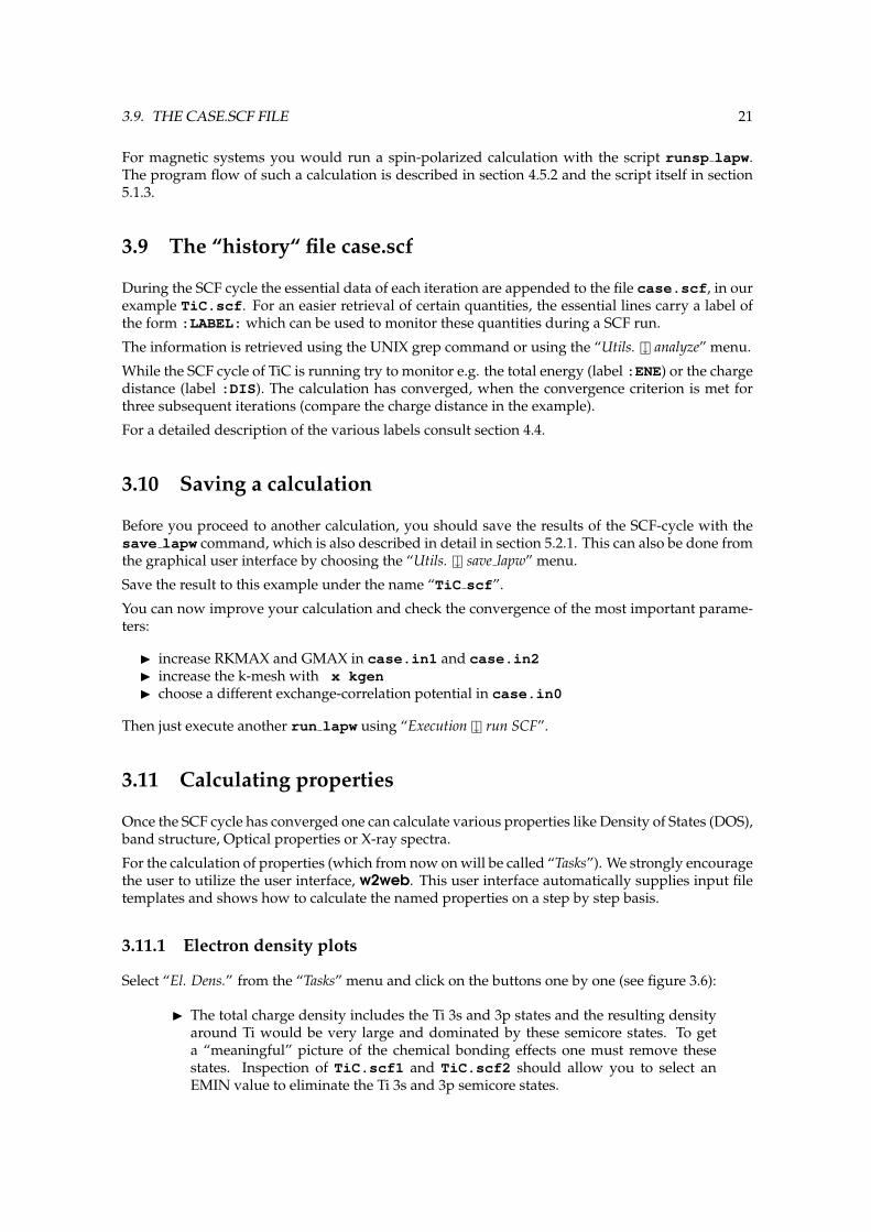
3.9 The “history“ file case.scf
During the SCF cycle the essential data of each iteration are appended to the file case.scf, in ourexample TiC.scf. For an easier retrieval of certain quantities, the essential lines carry a label ofthe form :LABEL: which can be used to monitor these quantities during a SCF run.
The information is retrieved using the UNIX grep command or using the “Utils. o analyze” menu.
While the SCF cycle of TiC is running try to monitor e.g. the total energy (label :ENE) or the chargedistance (label :DIS). The calculation has converged, when the convergence criterion is met forthree subsequent iterations (compare the charge distance in the example).
For a detailed description of the various labels consult section 4.4.
3.10 Saving a calculation
Before you proceed to another calculation, you should save the results of the SCF-cycle with thesave lapw command, which is also described in detail in section 5.2.1. This can also be done fromthe graphical user interface by choosing the “Utils. o save lapw” menu.
Save the result to this example under the name “TiC scf”.
You can now improve your calculation and check the convergence of the most important parame-ters:
I increase RKMAX and GMAX in case.in1 and case.in2I increase the k-mesh with x kgenI choose a different exchange-correlation potential in case.in0
Then just execute another run lapw using “Execution o run SCF”.
3.11 Calculating properties
Once the SCF cycle has converged one can calculate various properties like Density of States (DOS),band structure, Optical properties or X-ray spectra.
For the calculation of properties (which from now on will be called “Tasks”). We strongly encouragethe user to utilize the user interface, w2web. This user interface automatically supplies input filetemplates and shows how to calculate the named properties on a step by step basis.
3.11.1 Electron density plots
Select “El. Dens.” from the “Tasks” menu and click on the buttons one by one (see figure 3.6):
I The total charge density includes the Ti 3s and 3p states and the resulting densityaround Ti would be very large and dominated by these semicore states. To geta “meaningful” picture of the chemical bonding effects one must remove thesestates. Inspection of TiC.scf1 and TiC.scf2 should allow you to select anEMIN value to eliminate the Ti 3s and 3p semicore states.
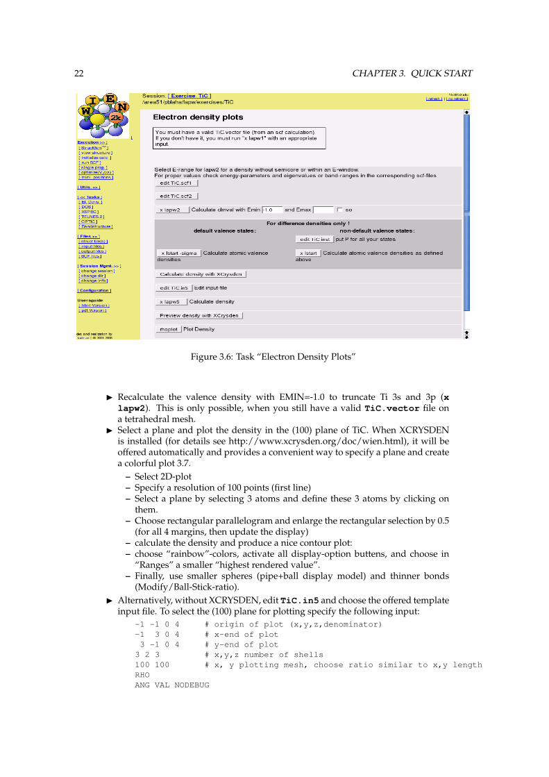
22 CHAPTER 3. QUICK START
Figure 3.6: Task “Electron Density Plots”
I Recalculate the valence density with EMIN=-1.0 to truncate Ti 3s and 3p (xlapw2). This is only possible, when you still have a valid TiC.vector file ona tetrahedral mesh.
I Select a plane and plot the density in the (100) plane of TiC. When XCRYSDENis installed (for details see http://www.xcrysden.org/doc/wien.html), it will beoffered automatically and provides a convenient way to specify a plane and createa colorful plot 3.7.
– Select 2D-plot– Specify a resolution of 100 points (first line)– Select a plane by selecting 3 atoms and define these 3 atoms by clicking on
them.– Choose rectangular parallelogram and enlarge the rectangular selection by 0.5
(for all 4 margins, then update the display)– calculate the density and produce a nice contour plot:– choose “rainbow”-colors, activate all display-option buttens, and choose in
“Ranges” a smaller “highest rendered value”.– Finally, use smaller spheres (pipe+ball display model) and thinner bonds
(Modify/Ball-Stick-ratio).I Alternatively, without XCRYSDEN, edit TiC.in5 and choose the offered template
input file. To select the (100) plane for plotting specify the following input:-1 -1 0 4 # origin of plot (x,y,z,denominator)-1 3 0 4 # x-end of plot3 -1 0 4 # y-end of plot3 2 3 # x,y,z number of shells100 100 # x, y plotting mesh, choose ratio similar to x,y lengthRHOANG VAL NODEBUG

3.11. CALCULATING PROPERTIES 23
ORTHO
For a detailed description of input options consult section 8.6.3I Calculate electron density (x lapw5)I Plot output (using rhoplot), after the first preview select a range zmin=-0.5 to
zmax=2
Figure 3.7: Electron density of TiC in (100) plane using Xcrysden
Compare the result with the electron density plotted in the (100) plane (see figure 3.8). The pro-gram gnuplot (public domain) must be installed on your computer. For more advanced graphicsuse your favorite plotting package or specify other options in gnuplot (see rhoplot lapw howgnuplot is called).

24 CHAPTER 3. QUICK START
Figure 3.8: Electron density of TiC in (100) plane
3.11.2 Density of States (DOS)
Select “Density of States (DOS)” from the “Tasks” menu and click on the buttons one by one:
I Calculate partial charges (x lapw2 -qtl). (This is only possible, when you stillhave a valid TiC.vector file on a tetrahedral mesh.)
I Edit TiC.int, choose the offered template input file and edit it to select: totalDOS, Ti-d, Ti-deg , Ti-dt2g , C-s and C-p-like DOS.
TiC-0.50 0.00200 1.500 0.003 EMIN, DE, EMAX, Gauss-broadening6 NUMBER OF DOS-CASES0 1 tot (atom,case,description)1 4 Ti d1 5 Ti eg1 6 Ti t2g2 2 C s2 3 C p
For a detailed description of input options consult section 8.1.3I Calculate DOS (x tetra).I Preview output using “dosplot”
If you want to use the supplied plotting interface dosplot2 to preview the results, the programgnuplot (public domain) must be installed on your computer.
The calculated DOS can be compared with figures 3.9 and 3.10. Together with the electron densitythe partial DOS allows you to analyse the chemical bonding (covalency between Ti−deg andC−p,non-bonding Ti− dt2g , charge transfer estimates,....)

3.11. CALCULATING PROPERTIES 25
Figure 3.9: Density of states of TiC
Figure 3.10: Density of states of TiC

26 CHAPTER 3. QUICK START
3.11.3 X-ray spectra
Select “X-Ray Spectra” from the “Tasks menu” and click on the buttons one by one:
I Calculate partial charges (x lapw2 -qtl). This is only possible, when you stillhave a valid TiC.vector file on a tetrahedral mesh. To reproduce this figure youwill have to increase the EMAX value in your TiC.in1 to 2.5 Ry and rerun x lapw1
I Edit TiC.inxs; choose the offered template. This template will calculate the LIII -spectrum of the first atom (Ti in this example) in the energy range between -2 and15 eV. For a detailed description of the contents of this input file refer to section8.10.3.
I Calculate spectraI Preview spectra
If you want to use the supplied plotting interface specplot to preview the results, the public domainprogram gnuplot must be installed on your computer. The calculated TiC Ti-LIII -spectrum can becompared with figure 3.11.
Figure 3.11: Ti LIII spectrum of TiC
3.11.4 Bandstructure
Select “Bandstructure” from the “Tasks” menu and click on the buttons one by one:
I Create the file TiC.klist band from the template in$WIENROOT/SRC templates/fcc.klist. (To calculate a bandstructure aspecial k-mesh along high symmetry directions is necessary. For a few crystalstructures template files are supplied in the SRC-directory, you can also useXCRYSDEN (save it as xcrysden.klist) to generate a k-mesh or type in your ownmesh.
I Calculate Eigenvalues using the “-band” switch (which changes lapw1.def suchthat the k-mesh is read from TiC.klist band and not from TiC.klist)Note: When you want to calculate DOS, charge densities or spectra after this bandstruc-ture, you must first recalculate the TiC.vector file using the “tetrahedral” k-mesh,because the k-mesh for the band structure plots is not suitable for calculations of suchproperties.

3.11. CALCULATING PROPERTIES 27
I Edit TiC.insp: insert the correct Fermi energy (which can be found in the savedscf-file) and specify plotting parameters. For comparison with figure 3.12 selectan energy-range from -13 to 8 eV.
I Calculate Bandstructure (x spaghetti).I Preview Bandstructure (needs ghostscript installed).
If you want to preview the bandstructure, the program ghostview (public domain) must be in-stalled on your computer. You can compare your calculated bandstructure with figure 3.12.
tic atom 0 size 0.40
W L Λ Γ ∆ X Z W K
EF
Ene
rgy
(eV
)
0.0
1.0
2.0
3.0
4.0
5.0
6.0
7.0
8.0
-1.0
-2.0
-3.0
-4.0
-5.0
-6.0
-7.0
-8.0
-9.0
-10.0
-11.0
-12.0
-13.0
Figure 3.12: Bandstructure of TiC
3.11.5 Bandstructure with band character plotting / full lines
Select again “Bandstructure” from the “Tasks” menu. We assume that you have already done thesteps described in the previous section (generate TiC.klist band and x lapw1 -band).
I Calculate partial charges (x lapw2 -qtl -band)Note: You have to calculate the partial charges for the new special k-mesh specified aboveand cannot use the partial charges from the DOS calculation.
I Edit TiC.insp: insert the correct Fermi energy (same as before) and specify plot-ting parameters. For ”band character plotting” (see figure 3.13) select ”line type= dots” and jatom=1, jtype=6 and jsize=0.2 (in the last input line) to produce acharacter plot of the Ti t2g-like character bands.
I Calculate Bandstructure (x spaghetti)I Preview BandstructureI To plot the bandstructure with full lines, calculate the irreducible representations
with ”x irrep” and select ”lines” in case.insp.
If you have case.irrep* or case.qtl* files from previous runs which do not fit to thepresent case.output1 file, you may get errors while running spaghetti. In this caseremove all case.irrep or case.qtl files.
You can compare your results with figure 3.13.

28 CHAPTER 3. QUICK START
tic atom 1D-t2g size 0.20
W L Λ Γ ∆ X Z W K
EF
Ene
rgy
(eV
)
0.0
1.0
2.0
3.0
4.0
5.0
6.0
7.0
8.0
-1.0
-2.0
-3.0
-4.0
-5.0
-6.0
-7.0
-8.0
-9.0
-10.0
-11.0
-12.0
-13.0
Figure 3.13: Bandstructure of TiC, showing t2g-character bands of Ti in character plotting mode
3.11.6 Volume Optimization
Select “Optimize (V,c/a)” from the “Execution” menu. Setup the shell script optimize.job scriptusing x optimize and volume variations of -10, -5, 0, +5 and +10%. Edit this file and uncommentthe x dstart line (remove the “#” character). Then run the optimize.job. When the job hasfinished, you should click on Plot and then preview the energy curve.
You should get an energy curve as in figure 3.14. On the screen you will find the fitting parametersfor the “equation of states” (Murnaghan, Birch-Murnaghan and the EOS2 equation, see sec. 9.10).This information is also written to TiC.outputeos.
Figure 3.14: Energy vs. volume curve for TiC

3.12. SETTING UP A NEW CASE 29
3.12 Setting up a new case
In order to setup a new case you need at least the following information:
I The lattice parameters (in Bohr or Angstroms) and angles,I the lattice type (primitive, face-centered, hexagonal,...) or spacegroup,I the position of all equivalent and inequivalent atoms in fractions of the unit cell.I Alternatively with the new StructGen you can specify the spacegroup and only the inequiv-
alent positions. The equivalent ones will be generated automatically.
Usually this information can be collected from the “International Tables of Crystallography” onceyou know the space group, the Wyckoff position and the internal free coordinates.
3.12.1 Manually setting up a new case
Usually for a new “case“ the input is not created from scratch, but one uses the struct file from asimilar case as pattern. Change into the lapw subdirectory and proceed as follows:
mkdir case newcd case newcp ../case old/case old.struct case new.struct
Now edit case new.struct (see section 4.3) as necessary (Note: this is a fixed formatted file,so all values must remain at their proper columns). Afterwards generate case new.inst usinginstgen lapw.
3.12.2 Setting up a new case using w2web
Use the menu Session Mgmt. o change session of w2web to create a new session (enter the name ofthe new session and click on “Create”). Then you should also create a new directory and “select”it..
When you select “Execution o StructGen”, you have several choices:
You can just specify the number of non-equivalent atoms and a template file will be created. InStructGen you simply specify the lattice (type or spacegroup), cell parameters and name and po-sitions of atoms. When you “save file and clean up” the new case.struct file and the case.instfile are created automatically.
Alternatively, you can use cif2struct or xyz2struct to convert a “cif”, “txt” or “xyz” fileinto the WIEN2k case.struct file. Check page 154 for more info on the specific file formats.
For more information on the StructGen refer to page 155.

30 CHAPTER 3. QUICK START

Part II
Detailed description of the files andprograms of the WIEN2k package
31


4 File structure and program flow
Contents4.1 Flow of input and output files . . . . . . . . . . . . . . . . . . . . . . . . . . . . . . 334.2 Input/Output files . . . . . . . . . . . . . . . . . . . . . . . . . . . . . . . . . . . . . 374.3 The case.struct.file . . . . . . . . . . . . . . . . . . . . . . . . . . . . . . . . . . . . . 384.4 The case.scf file . . . . . . . . . . . . . . . . . . . . . . . . . . . . . . . . . . . . . . 414.5 Flow of programs . . . . . . . . . . . . . . . . . . . . . . . . . . . . . . . . . . . . . 43
(for naming conventions see section 3.1)
4.1 Flow of input and output files
Each program is started with (at least) one command line argument, e.g.
programX programX.def
in which the arguments specifies a filename, in which FORTRAN I/O units are connected to unixfilenames. (See examples at specific programs). These “def“-files are generated automaticallywhen the standard WIEN2k scripts x, init lapw or run lapw are used, but may be tailored byhand for special applications. Using the option
x program -d
a def-file can be created without running the program. In addition each program reads/writes thefollowing files:
case.struct a “master“ input file, which is described below (Section 4.3)case.inX a specific input file, where X labels the program (see def-files for each program in chapter
6).case.outputX an output file
The programs of the SCF cycle (see figure 4.1) write the following files:
case.scfX a file containing only the most significant output (see description below).program.error error report file, should be empty after successful completion of a program (see
chapter 6)
33

34 CHAPTER 4. FILES AND PROGRAM FLOW
nece
ssar
yop
tiona
l
broy
d1
scf0
clm
sum
(old
)L
APW
0
LA
PW1
LC
OR
E
clm
cor
scfc
vect
or
scf1
kgen
LA
PW2
vsp
vns
clm
sc
clm
val
scf2
help
3*
scfm
(old
)
ME
RG
Esc
fM
IXE
R
clm
sum
(new
)
(new
)sc
fm
broy
d2
Figure 4.1: Data flow during a SCF cycle (programX.def, case.struct, case.inX, case.outputX andoptional files are omitted)

4.1. FLOW OF INPUT AND OUTPUT FILES 35
The following tables describe input and output files for the initialization programs nn, sgroup,symmetry, lstart, kgen, dstart (table 4.1), the utility programs tetra, irrep, spaghetti,aim, lapw7, elnes, lapw3, lapw5, xspec, optic, joint, kram, optimize and mini (table4.2) as well as for a SCF cycle of a non-spin-polarized case (table 4.2). Optional input and outputfiles are used only if present in the respective case subdirectory or requested/generated by aninput switch. The connection between FORTRAN units and filenames are defined in the respectiveprogramX.def files. The data flow is illustrated in Fig. 4.1.
program needs generatesnecessary optional necessary optional
NN nn.def case.outputnn case.struct nncase.struct
SGROUP case.struct case.outputsgroup case.struct sgroup
SYMMETRY symmetry.def case.outputs case.struct stcase.struct case.in2 st case.in2 st
LSTART lstart.def case.outputst case.rspupcase.struct case.rsp case.rspdncase.inst case.in0 st case.vsp st
case.in1 st case.vspdn stcase.in2 st case.sigmacase.inc stcase.inm stcase.inm restart
KGEN kgen.def case.outputkgencase.struct case.klist
case.kgenDSTART dstart.def case.outputd
case.struct case.clmsum(up)case.rsp(up) dstart.errorcase.in0 case.in0 stdcase.in1case.in2
Table 4.1: Input and output files of init programs
program needs generatesnecessary optional necessary optional
SPAGHETTI spaghetti.def case.qtl case.spaghetti ps case.spaghetti enecase.insp case.outputso case.outputspcase.struct case.irrep case.band.agrcase.output1
TETRA tetra.def case.outputtcase.int case.dos1(2,3)case.qtl case.dos1ev(1,2,3)case.kgen
LAPW3 lapw3.def case.output3case.struct case.rhocase.in2case.clmsum case.clmsum
LAPW5 lapw5.def case.sigma case.output5 case.rho.onedcase.struct case.rhocase.in5case.clmval
XSPEC xspec.def case.outputx case.coredenscase.inc case.dos1evcase.int case.xspeccase.vsp case.txspeccase.struct case.m1case.qtl case.m2
OPTIC optic.def case.outputopcase.struct case.symmatcase.mat diagcase.inopcase.vspcase.vector
JOINT joint.def case.outputjoint case.sigma intracase.injoint case.joint case.intra
continued on next page

36 CHAPTER 4. FILES AND PROGRAM FLOW
case.structcase.kgencase.weightcase.symmatcase.mat diag
KRAM kram.def case.epsilon case.elosscase.inkram case.sigmak case.sumrulescase.joint
OPTIMIZE case.struct case initial.struct optimize.job case vol xxxxx.structcase c/a xxxxx.struct
MINI mini.def case.scf mini case.outputM case.clmsum intercase.inM case.tmpM case.tmpM1case.finM case.constraint case.struct1case.scf case.clmhist case.scf mini1case.struct .min hess .minrestart
IRREP case.struct case.outputirrepcase.vector case.irrep
AIM case.struct case.outputaim case.critcase.clmsum case.surfcase.inaim
LAPW7 case.struct case.output7 case.abccase.vector case.gridcase.in7 case.psinkcase.vsp
QTL case.struct case.outputqcase.vector case.qtlcase.inqcase.vsp
Table 4.2: Input and output files of utility programs
program needs generatesnecessary optional necessary optional
LAPW0 lapw0.def case.clmup/dn case.output0 case.r2vcase.struct case.vrespsum/up/dn case.scf0 case.vcoulcase.in0 case.inm case.vsp(up/dn) case.vtotalcase.clmsum case.vns(up/dn)
ORB orb.def case.energy case.outputorb case.br1orbcase.struct case.vorb old case.scforb case.br2orbcase.inorb case.vorbcase.dmat orb.errorcase.vsp
LAPW1 lapw1.def case.vns case.output1 case.nsh(s)case.struct case.vorb case.scf1 case.nmat onlycase.in1 case.vector.old case.vectorcase.vsp case.energycase.klist
LAPWSO lapwso.def case.vorb case.vectorsocase.struct case.outputsocase.inso case.scfsocase.in1 case.energysocase.vector case.normsocase.vspcase.vnscase.energy
LAPW2 lapw2.def case.kgen case.output2 case.qtlcase.struct case.nsh case.scf2 case.weightcase.in2 case.weight case.clmval case.weighcase.vector case.weigh case.help03*case.vsp case.recprlist case.vrespvalcase.energy case.almblm
case.radwfLAPWDM lapwdm.def case.inso case.outputdm
case.struct case.scfdmcase.indm case.dmatcase.vector lapwdm.errorcase.vspcase.weighcase.energy
SUMPARA case.struct case.scf2p case.outputsumcase.clmval case.clmval
continued on next page

4.2. INPUT/OUTPUT FILES 37
case.scf2LCORE lcore.def case.vns case.outputc case.corewf
case.struct case.scfccase.inc case.clmcorcase.vsp lcore.error
After LCORE the case.scfX files are appended to case.scf and thecase.clmsum file is renamed to case.clmsum old (see run lapw)
MIXER mixer.def case.clmsum old case.outputm case.broyd*case.struct case.clmsc case.scfmcase.inm case.clmcor case.clmsumcase.clmval case.scf mixer.error
case.broyd1case.broyd2
After MIXER the file case.scfm is appended to case.scf, so that after an iteration iscompleted, the two essential files are case.clmsum and case.scf.
Table 4.3: Input and output files of main programs in an SCF cycle
4.2 Description of general input/output files
In the following section the content of the (non-trivial) output files is described:
case.almblm Contains the Alm, Blm, Clm coefficients of the wavefunctions (generated optional bylapw2).
case.broydX Contains the charge density of previous iterations if you use Broyden’s method formixing. They are removed when using save lapw. They should be removed by hand whencalculational parameters (RKMAX, kmesh, . . . ) have been changed, or the calculation crasheddue to a too large mixing and are restarted by using a new density generated by dstart.
case.clmcor Contains the core charge density (as σ(r) = 4πr2ρ(r) and has only a spherical part).In spin-polarized calculations two files case.clmcorup and case.clmcordn are used instead.
case.clmsc Contains the semi-core charge density in a 2-window calculation, which is no longerrecommended. In spin-polarized calculations two files are used instead: case.clmscup andcase.clmscdn.
case.clmsum Contains the total charge density in the lattice harmonics representation and asFourier coefficients. (The LM=0,0 term is given as σ(r) = 4πr2ρ(r), the others as r2ρLM (r);suitable for generating electron density plots using lapw5 when the TOT-switch is set,(see section 8.6). In spin-polarized calculations two additional files case.clmup andcase.clmdn contain the spin densities. Generated by dstart or mixer.
case.clmval Contains the valence charge density as r2ρLM (r); suitable for generating valence elec-tron density plots using lapw5 when the VAL-switch is set, (see 8.6). In spin-polarized cal-culations two files case.clmvalup and case.clmvaldn are used instead.
case.dmatup/dn Contains the density matrix generated by lapwdm for LDA+U, OP or Hybrid-DFT calculations.
case.dosX Contains the density of states (states/Ry) and corresponding energy (in Ry at the inter-nal energy scale) generated by tetra. X can be 1-3. Additional files case.dosXev containthe DOS in (states/eV) and the energy in eV with respect to EF.
case.help03X Contains eigenvalues and partial charges for atom number X.case.kgen This file contains the indices of the tetrahedra in terms of the list of k-points. It is used
in lapw2 (if EFMOD switch in case.in2 is set to TETRA, see 7.5.3) and in tetra.case.klist This file contains a list of k-points in the first BZ and represents a tetrahedral (special
point) mesh. It is generated in kgen and can either be inserted into the case.in1 file orused directly in kgen.
case.qtl Contains eigenvalues and corresponding partial charges (bandwise) in a form suitable fortetra and band structure plots with “band character”. The decomposition of these chargesis controlled by ISPLIT in case.struct.
case.radwf Contains the radial basis functions inside spheres (generated optional by lapw2).case.rho Contains the electron densities on a grid in a specified plane generated by lapw5. This
file can be used as input for your favorite contour or 3D plotting program.

38 CHAPTER 4. FILES AND PROGRAM FLOW
case.rsp Contains the atomic densities generated by lstart. They are used by dstart to gener-ate a first crystalline density (case.clmsum).
case.r2v Contains the exchange potential (in the lattice harmonics representation as r2 ∗ VLM (r)and as Fourier coefficients) in a form suitable for plotting with lapw5.
case.scf mini Contains the last scf-iteration of each individual time (geometry) step during a struc-tural minimization using mini. Thus this file contains a complete history of properties (en-ergy, forces, positions) during a structural minimization.
case.sigma Contains the atomic densities for those states with a “P” in case.inst. Generated inlstart and used for difference densities in lapw5.
case.spaghetti ps A ps file with the energy bandstructure plot generated by spaghetti.case.band.agr A xmgrace file with the energy bandstructure plot generated by spaghetti.case.vcoul Contains the Coulomb potential (in the lattice harmonics representation as r2 ∗ VLM (r)
and as Fourier coefficients) in a form suitable for plotting with lapw5.case.vorb Contains the orbital potential (in Ry) generated by orb for LDA+U or hybrid-DFT cal-
culations in form of a (2l+1,2l+1) matrix.case.vtotal Contains the total potential (in the lattice harmonics representation as r2 ∗ VLM (r) and
as Fourier coefficients) in a form suitable for plotting with lapw5.case.vector Binary file, contains the eigenvalues and eigenvectors of all k-points calculated in
lapw1. In spin-polarized calculations two files case.vectorup and case.vectordn areused instead. lapwso generates case.vectorso.
case.energy Contains the eigenvalues of all k-points calculated in lapw1. In spin-polarized calcu-lations two files case.vectorup and case.vectordn are used instead. lapwso generatescase.energyso.
case.vns Contains the non-spherical part of the total potential V. Inside the sphere the radial co-efficients of the lattice harmonics representation are listed (for L greater than 0), while forthe interstitial region the reanalyzed Fourier coefficients are given (see equ. (2.10)). In spin-polarized calculations two files case.vnsup and case.vnsdn are used instead.
case.vorbup/dn Contains the orbital dependent part of the potential in LDA+U, OP or Hybrid-DFT calculations. Generated in orb, used in lapw1.
case.vsp Contains the spherical part of the total potential V stored as r ∗ V (thus the first val-ues should be close to −2 ∗ Z). In spin-polarized calculations two files case.vspup andcase.vspdn are used instead.
4.3 The “master input“ file case.struct
The file case.struct defines the structure and is the main input file used in all programs. Weprovide several examples in the subdirectory
example struct file
If you are using the “Struct Generator” from the graphical user interface w2web, you don’t have tobother with this file directly! However, the description of the fields of the input mask can be foundhere.
Note: If you are changing this file manually, please note that this is a formatted file and the proper columnpositions of the characters are important! Use REPLACE instead of DELETE and INSERT during edit!
We start the description of this file with an abridged example for rutile TiO2 (adding line numbers):
--------------------- top of file ---------------------line #Titaniumdioxide TiO2 (rutile): u=0.305 1P LATTICE,NONEQUIV. ATOMS 2 2MODE OF CALC=RELA 38.6817500 8.6817500 5.5916100 90. 90. 90. 4
ATOM -1: X= 0.0000000 Y= 0.0000000 Z= 0.0000000 5

4.3. THE CASE.STRUCT.FILE 39
MULT= 2 ISPLIT= 8 6ATOM -1: X= 0.5000000 Y= 0.5000000 Z= 0.5000000Titanium NPT= 781 R0=.000022391 RMT=2.00000000 Z:22.0 7LOCAL ROT MATRIX: -.7071068 0.7071068 0.0000000 8
0.7071068 0.7071068 0.0000000 90.0000000 0.0000000 1.0000000 10
ATOM -2: X= 0.3050000 Y= 0.3050000 Z= 0.0000000MULT= 4 ISPLIT= 8
ATOM -2: X= 0.6950000 Y= 0.6950000 Z= 0.0000000ATOM -2: X= 0.8050000 Y= 0.1950000 Z= 0.5000000ATOM -2: X= 0.1950000 Y= 0.8050000 Z= 0.5000000Oxygen NPT= 781 R0=.000017913 RMT=1.60000000 Z: 8.0LOCAL ROT MATRIX: 0.0000000 -.7071068 0.7071068
0.0000000 0.7071068 0.70710681.0000000 0.0000000 0.0000000
16 SYMMETRY OPERATIONS: 111 0 0 0.00 120 1 0 0.00 130 0 1 0.00 14
1 151 0 0 0.000 1 0 0.000 0-1 0.00
2........
150 1 0 0.50
-1 0 0 0.500 0 1 0.50
16------------------ bottom of file ---------------------------
Interpretive comments on this file are as follows.
P all primitive lattices except hexagonal(trigonal lattice is also supported)
[a sin(γ), a cos(γ), 0], [0, b, 0], [0, 0, c]
F face-centered [a/2, b/2, 0], [a/2, 0, c/2], [0, b/2, c/2]B body-centered [a/2, -b/2, c/2],[a/2, b/2, -c/2], [-a/2, b/2, c/2]CXY C-base-centered (orthorhombic only) [a/2, -b/2, 0], [a/2, b/2, 0], [0, 0, c]CYZ A-base-centered (orthorhombic only) [a, 0, 0], [0, -b/2, c/2], [0, b/2, c/2]CXZ B-base-centered (orthorh. and monoclinic
symmetry)[a sin(γ)/2, a cos(γ)/2, -c/2], [0, b, 0], [a sin(γ)/2, acos(γ)/2, c/2]
R rhombohedral [a/√
3/2, -a/2, c/3],[a/√
3/2, a/2, c/3],[-a/√
3, 0, c/3]H hexagonal [
√3a/2, -a/2, 0],[0, a, 0],[0, 0, c]
Table 4.4: Lattice type, description and bravais matrix used in WIEN2k
line 1: format (A80)title (compound)
line 2: format (A4,23X,I3)lattice type, NAT
lattice type as defined in table 4.4. For definitions of the triclinic lattice seeSRC nn/dirlat.f
NAT number of inequivalent atoms in the unit cell
line 3: format (13X,A4)mode
RELA fully relativistic core and scalar relativistic valenceNREL non-relativistic calculation
line 4: format (6F10.6)a, b, c, α, β, γ

40 CHAPTER 4. FILES AND PROGRAM FLOW
a, b, c unit cell parameters (in a.u., 1 a.u. = 0.529177 A). In face- or body-centeredstructures the non-primitive (cubic) lattice constant, for rhombohedral (R) lat-tices the hexagonal lattice constants must be specified. (The following may helpyou to convert between hexagonal and rhombohedral specifications:ahex = 2cos(π−αrhomb
2)arhomb
chex = 3q
a2rhomb −
13a2
hex
and (for fcc-like lattices) arhomb = acubic/√
2α, β, γ angles between unit axis (if omitted, 90 is set as default). Set it only for P and
CXZ lattices
line 5: format (4X,I4,4X,F10.8,3X,F10.8,3X,F10.8)atom-index, x, y, z
atom-index
running index for inequivalent atoms
positive in case of cubic symmetrynegative for non-cubic symmetrythis is set automatically using symmetry
x,y,z position of atom in internal units, i.e. as positive fractions of unit cell parame-ters. (0 ≤ x ≤ 1; the positions in the unit cell are consistent with the conventionused in the International Tables of Crystallography 64. In face- (body-) centeredstructures only one of four (two) atoms must be given, eg. in Fm3m position 8cis specified with 0.25, 0.25, 0.25 and .75, 0.75, 0.75). For R lattice use rhombo-hedral coordinates. (To convert from hexagonal into rhombohedral coordinatesuse the auxiliary program hex2rhomb, which can be found in “Run Programso Other Goodies” from w2web):
~Xortho = ~Xhex
0@ 0 1 0√3
2−12
00 0 1
1A~Xrhomb = ~Xortho
0@ 1√3
1√3
−2√3
−1 1 01 1 1
1Aline 6: format (15X,I2,17X,I2)
multiplicity, isplit
multiplicity number of equivalent atoms of this kindisplit this is just an output-option and is used to specify the decomposition of the
lm-like charges into irreducible representations, useful for interpretation incase.qtl). This parameter is automatically set by symmetry:
0 no split of l-like charge1 p-z, (p-x, p-y) e.g.:hcp2 e-g, t-2g of d-electrons e.g.:cubic3 d-z2, (d-xy,d-x2y2), (d-xz,dyz) e.g.:hcp4 combining option 1 and 3 e.g.:hcp5 all d symmetries separate6 all p symmetries separate8 combining option 5 and 6-2 d-z2, d-x2y2, d-xy, (d-xz,d-yz)88 split lm like charges (for telnes)99 calculate cross-terms (for telnes)
>>>: line 5 must now be repeated MULT-1 times for the other positions of each equivalent atom accordingto the Wyckoff position in the “International Tables of Crystallography”.
line 7: format (A10,5X,I5,5X,F10.8,5X,F10.5,5X,F5.2)name of atom, NPT, R0, RMT, Z

4.4. THE CASE.SCF FILE 41
name ofatom
Use the chemical symbol. Positions 3-10 for further labeling of nonequivalentatoms (use a number in position 3)
NPT number of radial mesh points (381 gives a good mesh for LDA calculations,but for GGA twice as many points are recommended; always use an odd numberof mesh points!) the radial mesh is given on a logarithmic scale: r(n) = R0 ∗e[(n−1)∗DX]
R0 first radial mesh point (typically between 0.0005 and 0.00005)RMT atomic sphere radius (muffin-tin radius), can easily be estimated after running
nn (see 6.1) and are set automatically with setrmt lapw see 5.2.6). The follow-ing guidelines will be given here: Choose spheres as large as possible as thiswill save MUCH computer time. But: Use identical radii within a series of cal-culations (i.e. when you want to compare total energies) — therefore considerfirst how close the atoms may possibly come later on (volume or geometry op-timization); do NOT make the spheres too different (even when the geometrywould permit it), instead use the largest spheres for f-electron atoms, 10-20 %smaller ones for d-elements and again 10-20 % smaller for sp-elements; H is aspecial case, you may choose it much smaller (e.g. 0.6 and 1.2 for H and C) andsystems containing H need a much smaller RKMAX value (3-5) in case.in1.
Z atomic number
line 8-10: format (20X,3F10.7)
ROTLOC local rotation matrix (always in an orthogonal coordinate system). Transformsthe global coordinate system (of the unit cell) into the local at the given atomicsite as required by point group symmetry (see in the INPUT-Section 7.5.3 ofLAPW2). SYMMETRY calculates the point group symmetry and determinesROTLOC automatically. Note, that a proper ROTLOC is required, if the LMvalues generated by SYMMETRY are used. A more detailed description withseveral examples is given in the appendix A and sec. 10.3
>>>: lines 5 thru 10 must be repeated for each inequivalent atomline 11: format (I4)
nsym number of symmetry operations of space group (see International Tables ofCrystallography 64)If nsym is set to zero, the symmetry operations will be generated automaticallyby SYMMETRY.
line 12-14: format (3I2,F10.7)matrix, tau (as listed in the International Tables of Crystallography 64)
matrix matrix representation of (space group) symmetry operationtau non-primitive translation vector
line 15: format (I8)index of symmetry operation specified above
>>>: lines 12 thru 15 must be repeated for all other symmetry operations(the complete list is contained in sample inputs)
4.4 The “history“ file case.scf
During the self-consistent field (SCF) cycle the essential data are appended to the file case.scfin order to generate a summary of previous iterations. For an easier retrieval of certain quantitiesthe essential lines are labeled with :LABEL:, which can be used to monitor these quantities duringself-consistency as explained below. The most important :LABELs are

42 CHAPTER 4. FILES AND PROGRAM FLOW
:ENE total energy (Ry):DIS charge distance between last 2 iterations (
R|ρn − ρn−1|dr). Good convergence criterium.
:FER Fermi energy:FORxx force on atom xx in mRy/bohr (in the local (for each atom) carthesian coordinate system):FGLxx force on atom xx in mRy/bohr (in the global coordinate system of the unit cell (in the same
way as the atomic positions are specified)):DTOxx total difference charge density for atom xx between last 2 iterations:CTOxx total charge in sphere xx (mixed after MIXER):NTOxx total charge in sphere xx (new (not mixed) from LAPW2+LCORE):QTLxx partial charges in sphere xx:EPLxx l-like partial charges and “mean energies” in lower (semicore) energy window for atom
xx. Used as energy parameters in case.in1 for next iteration:EPHxx l-like partial charges and “mean energies” in higher (valence) energy window for atom xx.
Used as energy parameters in case.in1 for next iteration:EFGxx Electric field gradient (EFG) Vzz for atom xx:ETAxx Asymmetry parameter of EFG for atom xx:RTOxx Density for atom xx at the nucleus (first radial mesh point):VZERO Gives the total, Coulomb and xc-potential at z=0 and z=0.5 (meaningfull only for slab
calculations)
To check to which type of calculation a scf file corresponds use:
:POT Exchange-correlation potential used in this calculation:LAT Lattice parameters in this calculation:VOL Volume of the unit cell:POSxx Atomic positions for atom xx (as in case.struct):RKM Actual matrix size and resulting RKmax:NEC normalization check of electronic charge densities. If a significant amount of electrons
is missing, one might have core states, whose charge density is not completely confinedwithin the respective atomic sphere. In such a case the corresponding states should betreated as band states (using LOs).
For spin-polarized calculations:
:MMTOT Total spin magnetic moment/cell:MMIxx Spin magnetic moment of atom xx. Note, that this value depends on RMT.:CUPxx spin-up charge (mixed) in sphere xx:CDNxx spin-dn charge (mixed) in sphere xx:NUPxx spin-up charge (new, from lapw2+lcore) in sphere xx:NDNxx spin-dn charge (new, from lapw2+lcore) in sphere xx:ORBxx Orbital magnetic moment of atom xx (needs SO calculations and LAPWDM).:HFFxx Hyperfine field of atom xx (in kGauss).
One can monitor the energy eigenvalues (listed for the first k-point only), the Fermi-energy orthe total energy. Often the electronic charges per atom reflect the convergence. Charge transferbetween the various atomic spheres is a typical process during the SCF cycles: large oscillationsshould be avoided by using a smaller mixing parameter; monotonic changes in one direction sug-gest a larger mixing parameter.
In spin-polarized calculations the magnetic moment per atomic site is an additional crucial quan-tity which could be used as convergence criterion.
If a system has electric field gradients and one is interested in that quantity, one should monitorthe EFGs, because these are very sensitive quantities.
It is best to monitor several quantities, because often one quantity is converged, while another stillchanges from iteration to iteration. The script run lapw has three different convergence criteriabuilt in, namely the total energy, the atomic forces and the charge distance (see 5.1.2, 5.1.3).

4.5. FLOW OF PROGRAMS 43
We recommend the use of UNIX commands like :
grep :ENE case.scf or use “Analysis” from w2web
for monitoring such quantities.
You may define an alias for this (see sec. 11.2), and a csh-script grepline lapw is also availableto get a quantity from several scf-files simultaneously (sec. 5.2.15 and 5.3).
4.5 Flow of programs
The WIEN2k package consists of several independent programs which are linked via C-SHELLSCRIPTS described below.
The flow and usage of the different programs is illustrated in the following diagram (Fig. 4.2):
The initialization consists of running a series of small auxiliary programs, which generates theinputs for the main programs. One starts in the respective case/ subdirectory and defines thestructure in case.struct (see 4.3). The initialization can be invoked by the script init lapw(see sec. 3.7 and 5.1.2), and consists of running:
NN a program which lists the nearest neighbor distances up to a specified limit (defined by adistance factor f) and thus helps to determine the atomic sphere radii. In addition it is avery usefull additional check of your case.struct file (equivalency of atoms)
SGROUP determines the spacegroup of the structure defined in your case.struct file.SYMMETRY generates from a raw case.struct file the space group symmetry operations, deter-
mines the point group of the individual atomic sites, generates the LM expansion for thelattice harmonics and determines the local rotation matrices.
LSTART generates free atomic densities and determines how the different orbitals are treated inthe band structure calculations (i.e. as core or band states, with or without local orbitals,. . . ).
KGEN generates a k-mesh in the irreducible part of the BZ.DSTART generates a starting density for the scf cycle by a superposition of atomic densities
generated in LSTART.
Then a self-consistency cycle is initiated and repeated until convergence criteria are met (see 3.8and 5.1.3). This cycle can be invoked with a script run lapw, and consists of the following steps:
LAPW0 (POTENTIAL) generates potential from densityLAPW1 (BANDS) calculates valence bands (eigenvalues and eigenvectors)LAPW2 (RHO) computes valence densities from eigenvectorsLCORE computes core states and densitiesMIXER mixes input and output densities
4.5.1 Core, semi-core and valence states
In many cases it is desirable to distinguish three types of electronic states, namely core, semi-coreand valence states. For example titanium has core (1s, 2s, 2p), semi-core (3s, 3p) and valence (3d,4s, 4p) states. In our definition core states are only those whose charge is entirely confined insidethe corresponding atomic sphere. They are deep in energy, e.g., more than 7-10 Ry below the Fermienergy. Semi-core states lie high enough in energy (between about 1 and 7 Ry below the Fermienergy), so that their charge is no longer completely confined inside the atomic sphere, but has afew percent outside the sphere. Valence states are energetically the highest (occupied) states andalways have a significant amount of charge outside the spheres.

44 CHAPTER 4. FILES AND PROGRAM FLOW
old ρcoreρval( + )ρnew =
ρnew
ρval
Ek ψ k
ψ k Ek ψ k− 2+ V =
ρcore
VMT
Ecore
ψnl Enl ψnl=H
ρvalE < Ek F
= Σ ψψ∗k k
ρold
VC VXCV= +
VXC ρ LDA( )VC
2 = −8 Poissonπρ
ρ
k−mesh
LAPW0
ψnl Enl ψnl=H
SYMMETRYSGROUP
converged ?
no
MIXER
LAPW2
V
LAPW1
atomic calculation
LCORE
LAPWSO
STOPyes
atomic calculation
LSTARTNN
atomic densities
input files
DSTART
superposition of
atomic densities
ρ
check foroverlap. spheres
input filesstruct filesstruct files
KGEN
generation
add spin−orbit interaction
LAPWDMcalculates density matrix
ORBLDA+U, OP potentials
Figure 4.2: Program flow in WIEN2k

4.5. FLOW OF PROGRAMS 45
The energy cut-off specified in lstart during init lapw (usually -6.0 Ry) defines the separationinto core- and band-states (the latter contain both, semicore and valence). If a system has atomswith semi-core states, then the best way to treat them is with “local orbitals“, an extension of theusual LAPW basis. An input for such a basis set will be generated automatically. (Additional LOscan also be used for valence states which have a strong variation of their radial wavefunctions withenergy (e.g. d states in TM compounds) to improve the quality of the basis set, i.e. to go beyondthe simple linearization).
4.5.2 Spin-polarized calculation
For magnetic systems spin-polarized calculations can be performed. In such a case some steps aredone for spin-up and spin-down electrons separately and the script runsp lapw consists of thefollowing steps:
LAPW0 (POTENTIAL) generates potential from densityLAPW1 -up (BANDS) calculates valence bands for spin-up electronsLAPW1 -dn (BANDS) calculates valence bands for spin-down electronsLAPW2 -up (RHO) computes valence densities for spin-up electronsLAPW2 -dn (RHO) computes valence densities for spin-down electronsLCORE -up computes core states and densities for spin-up electronsLCORE -dn computes core states and densities for spin-down electronsMIXER mixes input and output densities
The use of spin-polarized calculations is illustrated for fcc Ni (section 10.2), one of the test casesprovided in the WIEN2k package.
4.5.3 Fixed-spin-moment (FSM) calculations
Using the script runfsm lapw -m XX it is possible to constrain the total spin magnetic momentper unit cell to a fixed value XX and thus force a particular ferromagnetic solution (which maynot correspond to the equillibrium). This is particularly useful for systems with several metastable(non-) magnetic solutions, where conventional spin-polarized calculation would not converge orthe solution may depend on the starting density. Additional SO-interaction is not supported.
Please note, that once runfsm lapw has finished, only case.vectordn is ok, butcase.vectorup is NOT the proper up-spin vector and MUST NOT be used for the calculationsof QTLs (and DOS). It must be regenerated by x lapw1 -up (see also the comments for iterativediagonalization in section 5.2.17).
4.5.4 Antiferromagnetic (AFM) calculations
Several considerations are necessary, when you want to perform an AFM calculation. Please havealso a look into $WIENROOT/SRC afminput/afminput test.
I Create a struct file of the non-magnetic (or ferro-magnetic) supergroup (run init lapw up tolstart). Name it case.struct supergroup. (For example for bcc Cr, this would be a structfile with the ordinary cubic lattice parameters, “B” type lattice and just one Cr at (0,0,0).)
I Next construct a unit cell which allows the desired AF ordering. For example for bcc Cryou must select a “P” lattice and specify both atoms, Cr1 at (0,0,0) and Cr2 at (.5,.5,.5), corre-sponding to a CsCl structure. Note, that it is important to label the two Cr atoms with “Cr1”and “Cr2”, since only then the symmetry programs can detect that those atoms should bedifferent (although they have the same Z). If sgroup has interchanged some axis, try to undo thesechanges, since afminput may not properly find the correct symmetry operations in such a case.
46 CHAPTER 4. FILES AND PROGRAM FLOW
I Edit case.inst and flip the spin of one of the AF atoms (i.e. invert the spin up and dnoccupation numbers). In addition you should set a zero moment (identical spin up and dnoccupations) for all “non-magnetic” atoms.
I Run init lapw. At the end AFMINPUT creates an input file for the program CLMCOPY.Depending on the presence of case.struct supergroup and the specific symmetry itmay/may not ask you to supply a symmetry operation/nonprimitive translation (see Sect.9.3 .
I Run runafm lapw. This script calls LAPW1 and LAPW2 only for spin-up but the corre-sponding spin-dn density is created by CLMCOPY according to the rules defined duringinitialization. This reduces the required cpu time by a factor of 2 (and in addition the scfcycle is much more stable).
I It is highly recommended that you save your work (save lapw) and check the results bycontinuing with a regular runsp lapw. If nothing changes (E-tot and other properties), thenyou are ok, otherwise make sure the scf calculation is well converged (-cc 0.0001 or better).Eventually the system may not want to be antiferromagnetic (but for instance it is ferrimag-netic!).
runafm lapw saves you more than a factor of 2 in in computer time, since only spin-up is cal-culated and in addition the scf-convergence may be MUCH faster. It works also with LDA+U(case.dmatup/dn are also copied), but does NOT work with Hybrid-DFT nor spin-orbit cou-pling, since this requires the presence of both vector files in the LAPWSO step.
4.5.5 Spin-orbit interaction
You can add spin-orbit interaction in LAPWSO (called directly after LAPW1) using a second-variational method with the scalar-relativistic orbitals (from LAPW1) as basis. The number ofeigenvalues will double since SO couples spin-up and dn states, so they are no longer separable.In addition, LOs with a “p1/2” radial basis can be added. (Kunes et al. 2001)
To assist with the generation of the necessary input files and possible changes in symmetry, a scriptinitso lapw exists. For non-spinpolarized cases nothing particular must be taken into accountand SO can be easily applied by running run lapw -so. It will automatically use the complexversion of LAPW2.
However, for spin-polarized cases, the SO interaction may change (lower) the symmetry depend-ing on how you choose the direction of magnetization and care must be taken to get a proper setup.initso lapw together with symmetso generates the proper symmetry.
Just a few hints what can happen:
I Suppose you have a cubic system and put the magnetization along [001]. This will createa tetragonal symmetry (and you can temporarely tell this to the initialization programs bychanging the respective lattice parameter c to a tetragonal system).
I If you put the magnetization along [111], this creates most likely a rhombohedral (or hexag-onal) symmetry. (Try to visualize this for a fcc lattice, XCRYSDEN is very usefull for thispurpose).
I Symmetry operations can be classified into operations which invert the magnetization,otherswhich leave it unchanged and some which do some arbitrary rotation. The programsymmetso (part of initso lapw) sorts these operations in the proper way.
I If you don’t have inversion symmetry in the original structure, you must not “add inversion”in KGEN.
The recommended way to include SO in the calculations is to run a regular scf calculation first,save the results, initialize SO and run another scf cycle including SO:

4.5. FLOW OF PROGRAMS 47
I run[sp] lapwI save lapw case nrelI initso lapwI run[sp] lapw -so
For spin-polarized systems you may want to add the “-dm” switch to calculate also the orbitalmagnetic moment.
4.5.6 Orbital potentials
In WIEN2kit is possible to go beyond standard LDA (GGA) and include orbital dependent po-tentials in methods like LDA+U or the ”Orbital-Polarization”, which are very usefull for stronglycorrelated systems.
To use these features you need to create input-files for LAPWDM and ORB (case.indm,case.inorb). You may copy a template from SRC templates, but must modify it according toyour needs. In particular you must select for which atoms and which orbitals (usually d-Orbitalsof late transition metal atoms or f-orbitals for 4f/5f atoms) you want to add such a potential andalso choose the proper U and J values for them. Once this is done, you can include this using the-orb switch. The density matrix (case.dmatup/dn) will be calculated after lapw2 in lapwdm, itwill be mixed in mixer (consistently with the “regular” charge density) and the orbital dependendpotentials will be calculated on orb (after lapw0). Note, you must run spin-polarized in order touse orbital potentials.
I runsp lapw -orb [-so]
If you want to force a non-magnetic solution you can constrain the spin-polarization to zero usingrunsp c lapw.
Without SO, case.vorbup/dn will be considered in LAPW1(c). With SO, it will be applied inLAPWSO (and allows coupling of nondiagonal spin-terms).
4.5.7 Exact-exchange and Hybrid functionals for correlated electrons
In WIEN2kit is also possible to go beyond standard LDA (GGA) and include on-site exact-exchange(Hartree-Fock), which is very usefull for strongly correlated systems. The exact-exchange/hybridmethods are implemented only inside the atomic spheres, therefore it is recommended to us themonly for localized electrons (see Tran et al. 2006 for details). They will NOT improve gaps in sp-semiconductors.
Examples of implemented functionals include:
I LDA-Hartree-FockFunctional 5 in case.in0. mode = EECE and fraction = 1 in case.ineece.
ELDA-HFxc [ρ] = ELDA
xc [ρ] + EHFx [Ψcorr]− ELDA
xc [ρcorr]
I LDA-Fock-αFunctional 5 in case.in0. mode = HYBR and fraction = α in case.ineece.
ELDA-Fock-αxc [ρ] = ELDA
xc [ρ] + α(EHF
x [Ψcorr]− ELDAx [ρcorr]
)

48 CHAPTER 4. FILES AND PROGRAM FLOW
I PBE-Fock-αFunctional 13 in case.in0. mode = HYBR and fraction = α in case.ineece.
EPBE-Fock-αxc [ρ] = EPBE
xc [ρ] + α(EHF
x [Ψcorr]− EPBEx [ρcorr]
)The PBE0 functional corresponds to α = 0.25.
I TPSS-H-Fock-αFunctional 27 in case.in0. mode = HYBR and fraction = α in case.ineece.
ETPSS-H-Fock-αxc [ρ] = ETPSS
xc [ρ] + α(EHF
x [Ψcorr]− ETPSSx [ρcorr]
)It is similar to PBE0, but uses the meta-GGA TPSS.
I B3PW91Functional 18 in case.in0. mode = HYBR and fraction = 0.2 in case.ineece.
EB3PW91xc [ρ] = ELDA
xc [ρ] + 0.2(EHF
x [Ψcorr]− ELDAx [ρcorr]
)+0.72
(EB88
x [ρ]− ELDAx [ρ]
)+0.81
(EPW91
c [ρ]− ELDAc [ρ]
)In addition to the input files which are necessary for an usual LDA or GGA calculation, theinput file case.ineece is necessary to start a calculation. You may copy a template fromSRC templates, but must modify it according to your needs. In particular you must select forwhich atoms and which orbitals (usually d-Orbitals of late transition metal atoms or f-orbitals for4f/5f atoms) you want to add such a potential and which type of functional you want to use.
A sample input for calculations with exact exchange is given below.
------------------ top of file: case.ineece ------------9.0 2 emin, natorb1 1 2 1st atom index, nlorb, lorb2 1 2 2nd atom index, nlorb, lorbHYBR HYBR / EECE mode0.25 fraction of exact exchange------------------ bottom of file ---------------------
Interpretive comments on this file are as follows:line 1: free formatemin, natom
emin lower energy cutoff, to be selected so that the energy of correlated statesis larger than emin
natorb number of atoms for which the exact exchange is calculated
line 2: free formatiatom(i), nlorb(i), (lorb(li,i), li=1,nlorb(i))
iatom index of atom in struct filenlorb number of orbital moments for which exact exchange shall be calcu-
latedlorb orbital numbers (repeated nlorb-times)
2nd line repeated natorb-times

4.5. FLOW OF PROGRAMS 49
line 3: free formatmode
HYBR means that LDA/GGA exchange will be replaced by exact exchangeEECE means that LDA/GGA exchange-correlation will be replaced by exact
exchange
line 4: free format
alpha This is the fraction of Hartree-Fock exchange (between 0 and 1)
As with LDA+U , hybrid functionals can be used only for spin-polarized calculations(runsp lapw with the switch -eece). runsp lapw will internally call runeece lapw, whichwill create all necessary additional input files: case.indm (case.indmc), case.inorb,case.in0eece, case.in2eece (case.in2ceece) and once this is done, calculates in a se-ries of lapw2/lapwdm/lapw0/orb calculations the corresponding orbital dependend potentials.
I runsp lapw -eece [-so]

50 CHAPTER 4. FILES AND PROGRAM FLOW

5 Shell scripts for running programs
Contents5.1 Job control . . . . . . . . . . . . . . . . . . . . . . . . . . . . . . . . . . . . . . . . . 515.2 Utility scripts . . . . . . . . . . . . . . . . . . . . . . . . . . . . . . . . . . . . . . . 545.3 Structure optimization . . . . . . . . . . . . . . . . . . . . . . . . . . . . . . . . . . 595.4 Phonon calculations . . . . . . . . . . . . . . . . . . . . . . . . . . . . . . . . . . . 635.5 Parallel Execution . . . . . . . . . . . . . . . . . . . . . . . . . . . . . . . . . . . . . 635.6 Getting on-line help . . . . . . . . . . . . . . . . . . . . . . . . . . . . . . . . . . . 695.7 Interface scripts . . . . . . . . . . . . . . . . . . . . . . . . . . . . . . . . . . . . . . 69
5.1 Job control (c-shell scripts)
In order to run WIEN2k several c-shell scripts are provided which link the individual programs tospecific tasks.
All available (user-callable) commands have the ending lapw so you can easily get a list of allcommands using
ls $WIENROOT/∗ lapw
in the directory of the WIEN2k executables. (Note: all of the more important commands have a link to ashort name omitting “ lapw”.) All these commands have at least one option, -h, which will print asmall help indicating purpose and usage of this command.
5.1.1 Main execution script (x lapw)
The main WIEN2kscript, x lapw or x, executes a single WIEN2kprogram. First it creates the corre-sponding program.def-file, where the connection between Fortran I/O-units and filenames aredefined. One can modify its functionality with several switches, modifying file definitions in caseof spin-polarized or complex calculations or tailoring special behaviour. All options are listed withthe help switch
x -h or x lapw -h
With some of the options the corresponding input files may be changed temporarely, but are setback to the original state upon completion.
51

52 CHAPTER 5. SHELL SCRIPTS
USAGE: x PROGRAMNAME [flags]
PURPOSE:runs WIEN executables: afminput,aim,broadening,clmcopy,clminter,dipan,dstart,eosfit,eosfit6,filtvec,init_xspec,hex2rhomb,irrep,joint,kgen,kram,lapw0,lapw1,lapw2,lapw3,lapw5,lapw7,lapwdm,lapwso,lcore,lorentz,lstart,mini,mixer,nn,pairhess,plane,qtl,optic,optimize,orb,rhomb_in5,sgroup,spaghetti,struct_afm_check,sumpara,supercell,symmetry,symmetso,telnes2,tetra,txspec,xspec, clmaddsub
FLAGS:-f FILEHEAD -> FILEHEAD for path of struct & input-files-t/-T -> suppress output of running time-h/-H -> help-d -> create only the def-file-up -> runs up-spin-dn -> runs dn-spin-sc -> runs semicore calculation-c -> complex calculation (no inversion symmetry present)-p -> run lapw1/2/so in parallel (needs .machines file)-orb -> runs lapw1 with LDA+U/OP or B-ext correction-it -> runs lapw1 with iterative diagonalization-nohns-> runs lapw1 without HNS-nmat_only-> runs lapw1 and yields only the matrixsize-emin X -> runs lapw2 with EMIN=X (in bin9_blaha.in2)-all X Y -> runs lapw2 with ALL and E-window X-Y (in bin9_blaha.in2)-qtl -> calculates QTL in lapw2-help_files -> creates case.helpXX files in lapw2-vresp-> creates case.vrespval (for TAU/meta-GGA) in lapw2-eece -> for hybrid-functionals (lapw0,lapw2,mixer,orb,sumpara)-band -> for bandstructures: unit 4 to 5 (in1), sets QTL and ROOT (in2)-fermi-> calculates Fermi energy and weights in lapw2-efg -> calculates lapw2 with EFG switch-so -> runs lapw2 with def-file for spin-orbit calculation-fft -> runs dstart only up to case.in0_std creation-super-> runs dstart and creates new_super.clmsum (and not case.clmsum)-sel -> use reduced vector file in lapw7-settol 0.000x -> run sgroup with different tolerance-sigma-> run lstart with case.inst_sigma (autogenerated) for diff.dens.USE: x -h PROGRAMNAME for valid flags for a specific program
Note: To make use of a scratch file system, you may specify such a filesystem in the environment variableSCRATCH (it may already have been set by your system administrator). However, you have to make surethat there is enough disk-space in the SCRATCH directory to hold your case.vector* and case.help*files.
5.1.2 Job control for initialization (init lapw)
In order to start a new calculation, one should make a new subdirectory and run all calculationsfrom there. At the beginning one must provide at least one file (see 3), namely case.struct(see 4.3) (case.inst can be created automatically on the “fly”, see 6.4.3), then one runs a series ofprograms using init lapw. This script is described briefly in chapter 4.5) and in detail in “Gettingstarted” for the example TiC (see chapter 3). You can get help with switch -h. All actions of thisscript are logged in short in :log and in detail in the file case.dayfile, which also gives you a“restart” option when problems occurred. In order to run init lapw starting from a specific pointon, specify -s PROGRAM.
init lapw supports a “batch” mode (non-interactive) for trivial cases AND experienced users.You can supply various options and specify spin-polarization, XC-potential, RKmax, k-mesh ormixing. See init lapw -h for more details. Changes to case.struct by nn will be accepted,but by sgroup will be neglected.
5.1.3 Job control for iteration (run lapw or runsp lapw)
In order to perform a complete SCF calculation, several types of scripts are provided with thedistribution. For the specific flow of programs see chapter 4.5.

5.1. JOB CONTROL 53
I For non-spinpolarized calculations use: run lapw,I for spin-polarized calculations use: runsp lapw.I for antiferromagnetic calculations use: runafm lapwI for FSM (fixed-spin moment) calculations use: runfsm lapwI for a spin-polarized setup, where you want to constrain the moment to zero (e.g. for LDA+U
calculations) use: runsp c lapw
Cases with/without inversion symmetry and with/without semicore or core states are handled au-tomatically by these scripts. All activities of these scripts are logged in short in :log (appended)and in detail together with convergence information in case.dayfile (overwriting the old “day-file“). You can always get help on its usage by invoking these scripts with the -h flag.
run lapw -h
PROGRAM: /zeus/lapw/WIEN2k/bin/run_lapw
PURPOSE: running the nonmagnetic scf-cycle in WIENto be called within the case-subdirectoryhas to be located in WIEN-executable directory
USAGE: run_lapw [OPTIONS] [FLAGS]
OPTIONS:-cc LIMIT -> charge convercence LIMIT (0.0000 e)-ec LIMIT -> energy convercence LIMIT (0.0001 Ry)-fc LIMIT -> force convercence LIMIT (0 mRy/a.u.)
default is -ec 0.0001; multiple convergence tests possible-e PROGRAM -> exit after PROGRAM ()-i NUMBER -> max. NUMBER (40) of iterations-s PROGRAM -> start with PROGRAM ()-r NUMBER -> restart after NUMBER (99) iterations (rm *.broyd*)-nohns NUMBER ->do not use HNS for NUMBER iterations-ql LIMIT -> select LIMIT (0.05) as min.charge for E-L setting in new in1-in1new N -> use "new" in1 file after N iter (rewrite in1 using scf info)
FLAGS:-h/-H -> help-I -> with initialization of in2-files to "TOT"-NI -> does NOT remove case.broyd* (default: rm *.broyd* after 60 sec)-p -> run k-points in parallel (needs .machine file [speed:name])-it -> use iterative diagonalizations (after first cycle)-it0 ->use iterative diagonalizations (also in first cycle)-so -> run SCF including spin-orbit coupling-renorm-> start with mixer and renormalize density-in1orig-> use case.in1_orig file (after a previous -in1new)
CONTROL FILES:.stop stop after SCF cycle.fulldiag force full diagonalizationcase.inm_vresp activates calculation of vresp files for meta-GGAs
ENVIRONMENT VARIBLES:SCRATCH directory where vectors and help files should go
Additional flags valid only for magnetic cases (runsp lapw) include:
-dm -> calculate the density matrix (when -so is set, but -orb is not)-eece -> use "exact exchange+hybrid" methods-orb -> use LDA+U, OP or B-ext correction-orbc -> use LDA+U correction, but with constant V-matrix
Calling run lapw (after init lapw) from the subdirectory case will perform up to 40 iterations(or what you specified with switch -i) unless convergence has been reached earlier. You can choosefrom three convergence criteria, -ec (the total energy convergence is the default and is set to 0.0001Ry for at least 3 iterations), -fc (magnitude of force convergence for 3 iterations, ONLY if yoursystem has “free” structural parameters!) or -cc (charge convergence, just the last iteration), andany combination can also be specified. Be careful with these criteria, different systems will requirequite different limits (e.g. fcc Li can be converged to µRy, a large unit cell with heavy magnetic

54 CHAPTER 5. SHELL SCRIPTS
atoms only to 0.1 mRy). You can stop the scf iterations after the current cycle by generating anempty file .stop (use eg. touch .stop in the respective case-directory).
The scf-cycle creates case.broyd* files which contain the ”charge-history”. Once run lapw hasfinished, you should usually ”save lapw” (see below) the results. When you continue with an-other run lapw without ”save lapw” (because the previous run did not fulfill the convergencecriteria or you want to specify a more strict criterium) the ”broyden-files” will be deleted unlessyou specify -NI.
With -e PROGRAM you can run only part of one scf cycle (e.g. run lapw0, lapw1 and lapw2),with -s PROGRAM you can start at an arbitrary point in the scf cycle (e.g. after a previous cyclehas crashed and you want to continue after fixing the problem) and continue to self-consistency.Before mixer is invoked, case.clmsum is copied to case.clmsum old, and the final “important“files of the scf calculation are case.clmsum and case.scf.
Invoking
run lapw -I -i 30 -fc 0.5
will first set in case.in2 the TOT-switch (if FOR was set) to save cpu time, then run up to 30 scf cyclestill the force criterion of 0.5 mRy/a.u. is met (for 3 consecutive iterations). Then the calculation ofall terms of the forces is activated (setting FOR in case.in2) for a final iteration.
The switch -in1new N preserves for N iteration the default case.in1 file, thus using the “old”WIEN97 scheme to select the energy parameters. After the first N iterations write in1 lapw iscalled and a new case.in1 file is generated, where the energy parameters are set according tothe :EPLxx and :EPHxx values of the last scf iteration and the -ql value (see sections 4.4 and 7.3).In this way you select the best possible energy-parameters and also additional LOs to improvethe linearization may be generated automatically. Note, however, that this option is potentiallydangerous if you have a “bad” last iteration (or large changes from one scf iteration to the next.The switch -in1orig can be used to switch back to the original (“old”) scheme.
Parallelization is described in Sec. 5.5.
Iterative diagonalization, which can significantly save computer time (in particular for cases with“few electrons” (like surfaces) and “large matrices (larger than 2000)” a factor 2-5 ! is possible), isdescribed in Sec. 7.3. It needs the case.vector file from the previous scf-iteration and this file iscopied to case.vector.old when the -it switch is set.
You can save computer time by performing the first scf-cycles without calculating the non-sphericalmatrix elements in lapw1. This option can be set for N iterations with the -nohns N switch.
If you have a previous scf-calculation and changed lattice parameters or positions (volume opti-mization or internal positions minimization), we recommend to use -renorm to renormalize thedensity prior to the first iteration.
For magnetic systems which are difficult to converge you can use the script runfsm lapw -m M(see section 4.5.3) for the execution of fixed-spin moment (FSM) calculations.
5.2 Utility scripts
5.2.1 Save a calculation (save lapw)
After self-consistency has been reached, the script
save lapw head of save filename

5.2. UTILITY SCRIPTS 55
saves case.clmsum, case.scf, case.dmat, case.vorb and case.struct under the newname and removes the case.broyd* files. Now you are ready to modify structural parametersor input switches and rerun run lapw, or calculate properties like charge densities (lapw5), totaland partial DOS (tetra) or energy bandstructures (spaghetti).
For more complicated situations, where many parameters will be changed, we have extendedsave lapw so that calculations can not only be saved under the head of save filename butalso a directory can be specified. If you use any of the possible switches (-a, -f, -d, -s) all input fileswill be saved as well (and can be restored using restore lapw).
Options to save lapw can be seen with
save lapw -h
Currently the following options are supported-h help-a save all input files as well-f force save lapw to overwrite previous saves-d directory save calculation in directory specified-s silent operation (no output)
5.2.2 Restoring a calculation (restore lapw)
To restore a calculation the script restore lapw can be used. This script restores the struct,clmsum, vorb and dmat files as well as all input files. Note: The input files will only be restoredwhen save lapw -d was used, i.e. when you have saved a calculation in an extra directory.
After restore lapw you can continue and either run an scf cycle (run lapw) or recreate thescf-potential (x lapw0) and the corresponding eigenvectors (x lapw1) for further tasks (DOS,electron density,...).
Options to restore lapw are:-h help-f force restore lapw to overwrite previous files-d directory restore calculation from directory specified-s silent operation (no output)-t only test which files would be restored
5.2.3 Remove unnecessary files (clean lapw)
Once a case has been completed you can clean up the directory with this command. Only the mostimportant files (scf, clmsum, struct, input and some output files) are kept. It is very important touse this command when you have finished a case, since otherwise the large vector and helpXX fileswill quickly fill up all your disk space.
5.2.4 Migrate a case to/from a remote computer (migrate lapw)
This script migrates a case to a remote computer (to be called within the case-dir). Needs workingssh/scp without password; local and remote case-dir must have the same name.
Call it within the desired case-dir as:
migrate lapw [FLAGS OPTIONS] [user@]host:path/case-dir
with the following options:

56 CHAPTER 5. SHELL SCRIPTS
-put -> transfer of files to a remote host (default)-get -> transfer of files from a remote host
-all -> the complete directory is copied-start -> only files to start an scf cycle are copied (default for put)-end -> only new files resulting from an scf cycle are copied
(default for get)-save savedir -> "save_lapw -d save_dir" is issued and only save_dir is copied
FLAGS:-h -> help-clean -> a clean_lapw is issued before copying-r -> files in source directory are removed after copying-R -> source directory (and all files) are removed after copying-s -> do it silent (in batch mode)-z -> gzip files before scp (slow network)
5.2.5 Generate case.inst (instgen lapw)
This script generates case.inst from a case.struct file. It can be used instead of the“Structure-generator” of w2web. Note: the label “RMT” is necessary in case.struct.
5.2.6 Set R-MT values in your case.struct file (setrmt lapw)
This perl-script executes x nn and uses its output to determine the atomic sphere radii (obeyingrecommended ratios for H, sp-, d- and f- elements). It is called automatically within init lapw oryou may call it separately using:
setrmt lapw case [-r X ]
where case gives the head of the case.struct file. You may specify a reduction of the RMTs byX percent in order to allow for structural optimizations. It creates case.struct setrmt.
5.2.7 Check for running WIEN jobs (check lapw)
This script searches for .running.* files within the current directory (or the directory specifiedwith “-d full path directory”) and then performs a ps command for these processes. If the specifiedprocess has not been found, it removes the corresponding .running.* file after confirmation(default) or immediately (when “-f” has been specified).
5.2.8 Cancel (kill) running WIEN jobs (cancel lapw)
This script searches for .running.* files within the current directory (or the directory specifiedwith “-d full path directory”) and then kills the corresponding process after confirmation (default)or immediately (when “-f” has been specified). It is particular usefull for killing “k-point parallel”jobs.
5.2.9 Extract critical points from a Bader analysis (extractaim lapw)
This script extracts the critical points (CP) after a Bader analysis (x aim (-c)) fromcase.outputaim. It sorts them (according to the density), removes duplicate CPs, converts unitsinto A, e/A3, ... and produces critical points ang.

5.2. UTILITY SCRIPTS 57
It is used with: extractaim lapw case.outputaim
5.2.10 scfmonitor lapw
This program was contributed by:
Hartmut EnkischInstitute of Physics E1bUniversity of DortmundDortmund, [email protected] make comments or report problems with this program to the WIEN-mailinglist. If necessary, we will
communicate the problem to the authors.
It produces a plot of some quantities as function of iteration number (a maximum of 6 quantities ispossible at once) from the case.scf file as specified on the commandline using analyse lapwand GNUPLOT. This plot is updated in regular intervals.
You can call scfmonitor lapw using:
scfmonitor lapw [-h] [-i n] [-f case.scf] [-p] arg1 [arg2 ..arg6]
-h help switch-i n show only the last n iterations-f scf-file use "scf-file" instead of the default "case.scf"-p produces file "scfmonitor.png" instead of X-window plotarg1,... arguments to monitor (like ":ENE" or ":DIS" , see analyse_lapw )
The scfmonitor can also be called directly from w2web using the ”Analyse” tool.
In order to have a reasonable behavior of scfmonitor the GNUPLOT window should stay in back-ground. This can be achieved by putting a line into your .Xdefaults file like:
gnuplot*raise: off
Note: It does not make sense to start scfmonitor before the first cycle has finished because no case.scfexists at this point.
5.2.11 analyse lapw
The script analyse lapw is usually called from scfmonitor lapw. It ”greps” from an scf-filethe specified arguments and produces analyse.out.
analyse lapw is called using:
analyse lapw [-h] scf-file arg1 [arg2 arg3 arg4 arg5 arg6]
-h help switchscf-file "scf-file" to analyse (there’s no default "case.scf" !)arg1,... arguments to analyse:
atom independend: :ENE :DIS :FER :MMT

58 CHAPTER 5. SHELL SCRIPTS
atom iii dependend: :CTOiii :CUPiii :CDNiii :NTOiii :NUPiii :NDNiii:DTOiii :DUPiii :DDNiii :RTOiii :EFGiii :HFFiii:MMIiii
vector quantities: :FORiii[x/y/z] :POSiii[x/y/z] :FGLiii[x/y/z]where magnitude z z is the default
For vector quantities like :FGLiii or :POSiii (usefull with case.scf mini) one can specify therespective coordinate by adding x/y/z to the corresponding labels.
5.2.12 Check parallel execution (testpara lapw)
testpara lapw is a small script which helps you to determine an optimal selection for the file.machines for parallel calculations (see sec. 5.5).
5.2.13 Check parallel execution of lapw1 (testpara1 lapw)
testpara1 lapw is a small script which determines how far the execution of lapw1para hasproceeded.
5.2.14 Check parallel execution of lapw2 (testpara2 lapw)
testpara2 lapw is a small script which determines how far the execution of lapw2para hasproceeded.
5.2.15 grepline lapw
Using
grepline lapw :label ’filename*.scf’ lines for tail or
grepline :label ’filename*.scf’ lines for tail
you can get a list of a quantity “:label” (e.g. :ENE for the total energy) from several scf files atonce.
5.2.16 initso lapw
initso lapw helps you to initialize the calculations for spin-orbit coupling. It creates all re-quired input files (case.inso, case.in2c). In a spinpolarized case SO may reduce symmetryor equivalent atoms may become non-equivalent, and the script calls symmetso and will help youto find proper symmetries and setup the respective input files. It is called using
initso lapw or
initso
and you should carefully follow the instructions and explanations of the script.

5.3. STRUCTURE OPTIMIZATION 59
5.2.17 vec2old lapw
vec2old lapw moves case.vector files to case.vector.old. Usually called automaticallyjust before lapw1 when the iterative diagonalization (run lapw -it) is specified. It also worksfor the k-parallel case including local $SCRATCH directories.
For runfsm lapw the sequence had to be changed and the switches -updn or -dnup forcesvec2old to COPY case.vectorup tocase.vectordn (and vice versa). In the runfsm lapwcase the corresponding case.vector*.old files are generated just AFTER lapw2/lapwdm andnot BEFORE lapw1. Thus after runfsm lapw has finished, the corresponding spin-up/dn vectorsare case.vector*.old and NOT case.vector*.
5.2.18 clmextrapol lapw
clmextrapol lapw extrapolates the charge density (case.clmsum/up/dn) from old to new po-sitions. It takes the density from the old positions (copied into old.clmsum) and subtracts anatomic superposition density (new super.clmsum) fom the old positions and adds an atomic su-perposition density fom the new ones (generated by dstart). If new super.clmsum (generatedautomatically by init lapw) is not present, it will be generated and for the next geometry step anextrapolation will take place.
It is usually called from “min lapw -ex” after a geometry step has finished and a new struct filehas been generated.
It can significantly reduce the number of scf-cycles for the new geometry step.
5.3 Structure optimization
5.3.1 Lattice parameters (Volume, c/a, lattice parameters)
The auxilliary program optimize (x optimize) generates from an existing case.struct (orcase initial.struct, which is generated at the first call of optimize) a series of struct fileswith various volumes (or c/a ratios, or other modified parameters) (depending on your input):
[1] VARY VOLUME with CONSTANT RATIO A:B:C[2] VARY C/A RATIO with CONSTANT VOLUME (tetr and hex lattices)[3] VARY C/A RATIO with CONSTANT VOLUME and B/A (orthorh lattice)[4] VARY B/A RATIO with CONSTANT VOLUME and C/A (orthorh lattice)[5] VARY A and C (2D-case) (tetragonal or hexagonal lattice)[6] VARY A, B and C (3D-case) (orthorhombic lattice)[7] VARY A, B, C and Gamma (4D-case) (monoclinic lattice)[8] VARY C/A RATIO and VOLUME (2D-case) (tetr and hex lattices)
It also produces a shell-script optimize.job which looks similar to:
#!/bin/csh -fforeach i ( \
tic_vol_-10.0 \tic_vol__-5.0 \tic_vol___0.0 \tic_vol___5.0 \tic_vol__10.0 \
)cp $i.struct tic.struct
# cp $i.clmsum tic.clmsum# x dstart# run_lapw -ec 0.0001 -in1new 3 -in1orig -renorm
run_lapw -ec 0.0001set stat = $statusif ($stat) then
echo "ERROR status in" $i
60 CHAPTER 5. SHELL SCRIPTS
exit 1endifsave_lapw $i
# save_lapw -f -d XXX $iend
You may modify this script according to your needs (use runsp lapw or even min lapw, specify dif-ferent convergence parameters, save into a directory to separate e.g. “gga” and “lda” results, acti-vate the line “x dstart” or “ cp $i.clmsum case.clmsum” to use a previously saved clmsumfile, e.g. from a calculation with smaller RKmax, ...)
Note: You must have a case.clmsum file (either from init lapw or from a previous scf calculation) inorder to run optimize.job.
After execution of this script you should have a series of scf-files with energies corresponding to themodified parameters, which should allow you to find the corresponding equillibrium parameters.For the volume optimization an analysis tool is available, other tools are under development).
Using the script grepline (or the “Analysis o Analyze multiple SCF-files” menu of w2web) youget a summary of the total energy vs. volume (c/a). The file case.analysis can be used ineplot lapw to find the minimum total energy and the equilibrium volume (c/a). Supportedequation of states include the EOS2, Murnaghan and Birch-Murnaghan EOS.
grepline :ENE ’*.scf’ 1 > case.analysisgrepline :VOL ’*.scf’ 1 >> case.analysis
Using such strategies also higher-dimensional optimizations (e.g. c/a ratio and volume) are possi-ble in combination with the -d option of save lapw.
For optimization of more degrees of freedom (2-4 lattice parameters), you can use the correspond-ing option and for analysis of the data the script parabolfit lapw together with the programeosfit6. It performs a non-linear least squares fit, using a parabolic fit-function in your variablesand get an analytic description of your energy surface. Please note, this is only a harmonic fit (noodd or higher terms) and the description may not be very good if your parameter range is largeand/or the function is quite anharmonic, or you suffer from numerical noise.
For the determination of elastic constants see the description of ELAST in sec 8.14.
5.3.2 Minimization of internal parameters (min lapw)
Most of the more complicated structures have free internal structural parameters, which can eitherbe taken from experiment or optimized using the calculated forces on the nuclei. The shell scriptmin lapw, together with the program mini, determines the equilibrium position of all individualatoms automatically (obeying the symmetry constraints of a certain space group).
A typical sequence of commands for an optimization of the internal positions would look like:
I Generate struct fileI init lapwI run lapw -fc 1 [another runXX script or additional options are of course also possible] (this
may take some time)I Inspect the scf file whether you have significant forces (usually at least .gt. 5 mRy/bohr),
otherwise you are more or less at the optimal positions (An experienced user may omit therun lapw step and proceed directly from init lapw to the next step)
I min lapw [options] (this may take some time)
– generates default case.inM (if not present) by:

5.3. STRUCTURE OPTIMIZATION 61
∗ x pairhess; cp case.inM st case.inM ; cp .minpair .min hess ; cp .minpair .minrestart(setting up the PORT minimization option). This step is also done automatically inminimizations using w2web.
∗ when -nohess is specified, it will generate case.inM from SRC templates with theNEW1 option.
Without -NI switch min lapw performs an initialization first:
I removes ”histories” (case.broyd*, case.tmpM) if present;I copies .min hess to .minrestart (if present from previous min lapw or x pairhess).
When case.scf is not present, an scf-cycle will be performed first, otherwise the correspondingforces are extracted into case.finM and mini generates a new case.struct with modifiedatomic positions. The previous step is saved under case 1/2/3.... Then a new scf-cycle isexecuted and this loop continues until convergence (default: forces below 2mRy/bohr) is reached.The last iteration of each geometry step is appended to case.scf mini, so that this file containsthe complete history of the minimization and can be used to monitor the progress (grep :ENE *mini;or :FORxxx ...).
By default (unless switch -noex is specified), min will call the script clmextrapol lapw after thefirst geometry step and try to extrapolate the charge density to the new positions. This procedureusually significantly reduces the number of scf-cycles and is thus highly recommended.
mini requires an input file case.inM (see Sec. 8.15) which is created automatically and MUSTNOT be changed while min lapw is running (except the force tolerance, which terminates theoptimization).
We recommend the PORT minimization method, a reverse-communication trust-region Quasi-Newton method from the Port library, which seems to be stable, efficient and does not dependtoo much on the users input (DELTAs, see below with NEWT). The PORT option also produces afile .min hess, which contains the (approximate) Hessian matrix (lower-triangle Cholesky factor)If you restart a minimization with different k-points, RMT, RKmax, ... or do a similar calculation(eg. for a different volume, ...) it will be copied to .minrestart (unless -nohess is specified), sothat you start with a reasonable approximation for the Hessian. When using PORT you may alsowant to check its progress using
grep :LABEL case.outputM
where :LABEL is :ENE (should decrease), :GRAD (should also go down, but could sometimes alsogo up for some time as long as the energy still decreases), :MIN (provides a condensed summaryof the progress), :WARN may indicate a problem), :DD (provides information about the step sizesand mode used). Some general explanations are:1) The algorithm takes steps along what it considers are good directions (using some internal logic),provided that these steps are smaller than what is called the trust-region radius. After a good step(e.g. large energy decrease) it expands the trust-region; after a bad one it reduces it. Sometimes itwill try too large a step then have to reduce it, so the energy does not always go down. You can seethis by using ”:DD” and “:MIN” .2) A grep on :MIN gives a condensed progress output, in which the most significant terms areE (energy in some rescaled units), RELDF (last energy reduction), PRELDF (what the algorithmpredicted for the step), RELDX (RMS change in positions in Angstroms) and NPRELDF (predictedchange in next cycle). Near the solution RELDF and RELDX should both become small. However,sometimes you can have soft modes in your structure in which case RELDX will take a long timebefore it becomes small.3) A warning that the step was reduced due to overlapping spheres if it happens only once (ortwice) is not important; the algorithm tested too large a step. However, if it occurs many times itmay indicate that the RMT’s are too big.

62 CHAPTER 5. SHELL SCRIPTS
4) A warning ”CURVATURE CONDITION FAILED” indicates that you are still some distance fromthe minimum, and the Hessian is changing a lot. If you see many of these, it may be that the forcesand energy are not consistent.
Sometimes PORT gets ”stuck” (often because of inconsistencies of energy and forces due to in-sufficient scf convergence or a very non-harmonic potential energy surface). A good alternative isNEW1, which is a ”sophisticated” steepest-descent method with optimized step size. It can be veryefficient in certain cases, but can also be rather slow when the potential energy surface is rather flatin one, but steep in another direction (eg. a weakly bound molecule on a surface, but constrainingthe sensitive parameters, like the bond distance of the molecule, may help).
Another alternative is NEWT, where one must set proper ”DELTAs” and a ”FRICTION” for eachatom. Unfortunately, these DELTAs determine crucially how the minimization performs. Too smallvalues lead to many (unnecessary) ”geometry steps”, while too large DELTAs can even lead todivergence (and finally to a crash). Thus you MUST control how the minimization performs. Werecommend the following sequence after 2-3 geometry steps:
grep :ENE *mini:ENE : ********** TOTAL ENERGY IN Ry = -2994.809124:ENE : ********** TOTAL ENERGY IN Ry = -2994.813852:ENE : ********** TOTAL ENERGY IN Ry = -2994.818538
Good, since the total energy is decreasing.
grep :FGL001 *mini:FGL001: 1.ATOM 0.000 0.000 18.219:FGL001: 1.ATOM 0.000 0.000 12.375:FGL001: 1.ATOM 0.000 0.000 7.876
Good, since the force (only a force along z is present here) is decreasing reasonably fast towardszero. You must check this for every atom in your structure.
When you detect oszillations or too small changes of the forces during geometry optimization, youwill have to decrease/increase the DELTAs in case.inM and rm case.tmpM. (NOTE: You mustnot continue with modified DELTAs but keeping case.tmpM.) Alternatively, stop the minimiza-tion (touch .minstop and wait until the last step has finished), change case.inM and restart.
You can get help on its usage with:
min -h or min lapw -h
PROGRAM: min
USAGE: min [OPTIONS]
OPTIONS:-j JOB -> job-file JOB (default: run_lapw -I -fc 1. -i 40 )-noex -> does not extrapolate the density for next geometry step-p -> adds -p (parallel) switch to run_lapw-it -> adds -it (iterative diag.) switch to run_lapw-sp -> uses runsp_lapw instead of run_lapw-nohess -> removes .minrestart (initial Hessian) from previous minimization-m -> extract force-input and execute mini (without JOB) and exit-mo -> like -m but without copying of case.tmpM1 to case.tmpM-h/-H -> help-NI -> without initialization of minimization (eg. continue after a crash)-i NUMBER -> max. NUMBER (50) of structure changes-s NUMBER -> save_lapw after NUMBER of structure changes
CONTROL FILES:.minstop stop after next structure change
For instance for a spin-polarized case, which converges more difficultly, you would use:
min -j ‘‘runsp lapw -I -ex -fc 1.0 -i 60’’

5.4. PHONON CALCULATIONS 63
5.4 Phonon calculations
Calculations of phonons is based on a program PHONON by K.Parlinski, which runs under MS-Windows and must be ordered separately (see http://wolf.ifj.edu.pl/phonon/ )
You would define the structure of your compound in PHONON together with a supercell of suf-ficient size (e.g. 64 atoms). PHONON will then generate a list of necessary displacements of theindividual atoms. The resulting file case.d45 must be transfered to UNIX. Here you would runWIEN2k-scf calculations for all displacements and collect the resulting forces, which will be trans-fered back to PHONON (case.dat and/or case.dsy). With these force information PHONONcalculates phonon at arbitrary q-vectors together with several thermodynamic properties.
5.4.1 init phonon lapw
init phonon lapw uses case.d45 from PHONON and creates subdirectories case XX andcase XX.struct files for all required displacements. It allows you to define globally RMT val-ues for the different atoms and initializes all cases individually (or copies the files from the firstcase). In low symmetry cases we recommend to use P1 symmetry for all cases and thus just oneinit lapw, while for higher symmetry a separate initialization is required (but computational effortis reduced). Please use maily nn to reduce equivalent atoms. sgroup might change the unitcelland than the collection of forces into the original supercell is quite difficult.
A script run phonon has been created. Modify it according to your needs (parallelization,....) andrun all cases to selfconsistency.
Note that good force convergence is essential (at least 0.1 mRy/bohr) and if your structure hasfree parameters, either very good equillibrium positions must have been found before, or evenbetter, use both, positive and negative displacements to average out any resulting error from non-equillibrium positions.
5.4.2 analyse phonon lapw
init phonon lapw uses the resulting scf files and generates the “Hellman-Feynman”-file re-quired by PHONON. When you have positive and negative displacements an automatic averagingwill be performed. The resulting case.dat and case.dsy filse should be transfered back to MS-Windows and imported into PHONON.
5.5 Running programs in parallel mode
This section describes two methods for running WIEN2k on parallel computers.
One method, parallelizing k-points over processors, utilizes c-shell scripts, NFS-file system andpasswordless login ((public/private keys). This method works with all standard flavors of Unixwithout any special requirements. The parallelization is very efficient even on heterogeneous com-puting environments, e. g. on heterogeneous clusters of workstations, but also on dedicated paral-lel computers and does NOT need large network bandwidth.
The other parallelization method, which comes new with version WIEN2k 07.3, is based on finegrained methods, MPI and SCALAPACK. It is especially useful for larger systems, if the requiredmemory size is no longer available on a single computer or when more processors than k-pointsare available. It requires a fast network (at least Gb-Ethernet, better Myrinet or Infiniband) ora shared memory machine. Although not as efficient as the simple k-point parallelization, thecurrent mpi-version has been enhanced a lot and shows very good scaling with the number of

64 CHAPTER 5. SHELL SCRIPTS
processors for most parts. In any case, the number of processors and the size of the problem (num-ber of atoms, matrixsize due to the plane wave basis) must be compatible and typically [NMAT /sqrt(processors)] .gt. 2000 should hold.
The k-point parallelization can use a dynamic load balancing scheme and is therefore usable also onheterogeneous computing environments like networks of workstations or PCs, even if interactiveusers contribute to the processors’ work load.
If your case is large enough, but you still have to use a few k-points, a combination of both paral-lelization methods is possible (always use k-point parallelism if you have more than 1 k-point).
5.5.1 k-Point Parallelization
Parts of the code are executed in parallel, namely LAPW1, LAPWSO, LAPW2, LAPWDM, andOPTIC. These are the numerically intensive parts of most calculations.
Parallelization is achieved on the k-point level by distributing subsets of the k-mesh to differentprocessors and subsequent summation of the results. The implemented strategy can be used bothon a multiprocessor architecture and on a heterogeneous (even multiplatform) network.
To make use of the k-point parallelization, make sure that your system meets the following require-ments:
NFS: All files for the calculation must be accessible under the same name and path. Therefore youshould set up your NFS mounts in such a way, that on all machines the path names are thesame.
Remote login: rlogin or ssh to all machines must be possible without specifying a password.Therefore you must either edit your .rhosts file to include all machines you intend to use(not necessary for a shared memory machine), or correctly specify public/private keys forssh. This can be done by running “ssh-keygen -t rsa” and copying the id rsa.pubkey into /.ssh/authorized keys at the remote sites.The command for launching a remote shell is platform dependent, and usually can be ’ssh’,’rsh’ or ’remsh’. It should be specified during installation when siteconfig lapw is exe-cuted (see chapter 11).
5.5.2 MPI parallelization
Fine grained MPI parallel versions are available for the programs lapw0, lapw1, and lapw2.This parallelization method is based on parallelization libraries, including MPI, ScaLapack, andPBlas. The required libraries are not included with WIEN2k. On parallel computers, however, theyare usually installed. Otherwise, free versions of these libraries are available1.
The parallelization affects the naming scheme of the executable programs: the fine grained par-allel versions of lapw0/1/2 are called lapw0 mpi, lapw1[c] mpi, and lapw2[c] mpi. Theseprograms are executed by calls to the local execution environments, as in the sequential case, bythe scripts x, lapw0para, lapw1para, and lapw2para. On most computers this is done bycalling mpirun and should also be configured using siteconfig lapw.
5.5.3 How to use WIEN2k as a parallel program
To start the calculation in parallel, a switch must be set and an input file has to be prepared by theuser.
1http://www-unix.mcs.anl.gov/mpi/mpich, http://www.netlib.org/scalapack

5.5. PARALLEL EXECUTION 65
I The switch -p switches on the parallelization in the scripts x and run lapw.I In addition to this switch the file .machines has to be present in the current working direc-
tory. In this file the machine names on which the parallel processes should be launched, andtheir respective relative speeds must be specified.
If the .machines file does not exist, or if the -p switch is omitted, the serial versions of the pro-grams are executed.
Generation of all necessary files, starting of the processes and summation of the results is doneby the appropriate scripts lapw1para, lapwsopara,lapwdmpara and lapw2para (when using-p), and parallel programs lapw0 mpi, lapw1 mpi, and lapw2 mpi (when using fine grainedparallelization has been selected in the .machines file).
5.5.4 The .machines file
The following .machines file describes a simple example. We assume to have 5 computers, (al-pha, ... epsilon), where epsilon has 4, and delta and gamma 2 cpus. In addition, gamma, delta andepsilon are 3 times faster than alpha and beta.:
# This is a valid .machines file#granularity:11:alpha1:beta3:gamma:2 delta3:delta:1 epsilon:4residue:delta:2lapw0:gamma:2 delta:2 epsilon:4
To each set of processors, defined by a single line in this file, a certain number of k-points is as-signed, which are computed in parallel. In each line the weight (relative speed) and computers arespecified in the following form:
weight:machine name1:number1 machine name2:number2 ...
where weight is an integer (e.g. a three times more powerful machine should have a three timeshigher weight). The name of the computer is machine name[1/2/...], and the number of pro-cessors to be used on these computers are number[1/2/...]. If there is only one processor on agiven computer, the :1 may be omitted. Empty lines are skipped, comment lines start with #.
Assuming there are 8 k-points to be distributed in the above example, they are distributed as fol-lows. The computers alpha and beta get 1 each. Two processors of computer gamma and one pro-cessor of computer delta cooperate in a fine grained parallelization on the solution of 3 k-points,and one processor of computer delta plus four processors of computer epsilon cooperate onthe solution of 3 k-points. If there were additional k-points, they would be calculated by the firstprocessor (or set of processors) becoming available. With higher numbers of k-points, this methodensures dynamic load balancing. If a processor is busy doing other (e. g., interactive) work, theoverall calculation will not stall, but most of its work will be done by other processors (or sets ofprocessors using MPI). This is, however, not an implementation for fail safety: if a process doesnot terminate (e. g., due to shutdown of a computer) the calculation will never terminate. It is upto the user to handle with such hardware failures by modifying the .machines file and restartingthe calculation at the appropriate point.
During the run of lapw1para the file .processes is generated. This file is used by lapw2parato determine which case.vector* to read.

66 CHAPTER 5. SHELL SCRIPTS
By default lapw1para will generate approximately 3 vector-files per processor, if enough k-pointsare available for distribution. The factor 3 is called “granularity” and allows for some load bal-ancing in heterogeneous environments. If you can be sure that load balancing is not an issue (eg.because you use a queuing-system and can be sure that you will get 100% of the cpus for your jobs)it is recommended to set
granularity:1
for best performance.
On shared memory machines it is advisable to add a “residue machine” to calculate the surplus(residual) k-points (given by the expression MOD(klist,
∑j newweightj) and rely on the operating
system’s load balancing scheme. Such a “residue machine” is specified as
residue:machine name:number
in the .machines file.
Alternatively, it is also possible to distribute the remaining k-points one-by-one (and not in onejunk) over all processors. The option
extrafine:1
can be set in the .machines file.
When using “iterative diagonalization” or the $SCRATCH variable (set to a local direc-tory), the k-point distribution must be “fixed”. This means, the ratio (k-points / processors) mustbe integer and granularity:1 should be set.
The line
lapw0:gamma:2 delta:2 epsilon:4
defines the computers used for running lapw0 mpi. In this example the 6 processors of the com-puters gamma, delta, and epsilon run lapw0 mpi in parallel.
If fine grained parallelization is used, each set of processors defined in the .machines file is con-verted to a single file .machine[1/2/...], which is used in a call to mpirun (or another parallelexecution environment).
When using a queuing system (like PBS, LoadLeveler or SUN-Gridengine) one can only requestthe NUMBER of processors, but does not know on which nodes the job will run. Thus a “static”.machines file is not possible. On can write a simple shell script, which will generate this file onthe fly once the job has been started and the nodes are assigned to this job. Examples can be foundat our web-site “http://www.wien2k.at/reg users/faq”.
5.5.5 How the list of k-points is split
In the setup of the k-point parallel version of LAPW1 the list of k-points in case.klist (Note, thatthe k-list from case.in1 cannot be used for parallel calculations) is split into subsets according to theweights specified in the .machines file:
newweighti =
⌊weighti ∗ klist
granularity ∗∑
j weightj
⌋

5.5. PARALLEL EXECUTION 67
where newweighti is the number of k-points to be calculated on processor i. newweighti is alwaysset to a value greater equal one.
A loop over all i processors is repeated until all k-points have been processed.
Speedup in a parallel program is intrinsically dependent on the serial or parallel parts of the codeaccording to Amdahl’s law:
speedup =1
(1− P ) + PN
whereas N is the number of processors and P the percentage of code executed in parallel.
In WIEN2k usually only a small part of time is spent in the programs lapw0, lcore and mixerwhich is very small (negligible) in comparison to the times spent in lapw1 and lapw2. The timefor waiting until all parallel lapw1 and lapw2 processes have finished is important too. For agood performance it is therefore necessary to have a good load balancing by estimating properlythe speed and availability of the machines used. We encourage the use of testpara lapw or “Utils.o testpara” from w2web to check the k-point distribution over the machines before actually runningthe programs in parallel.
While running lapw1 and lapw2 in parallel mode, the scripts testpara1 lapw (see 5.2.13) andtestpara2 lapw (see 5.2.14) can be used to monitor the succession of parallel execution.
5.5.6 Flow chart of the parallel scripts
To see how files are handled by the scripts lapw1para and lapw2para refer to figures 5.1 and5.2. After the lapw2 calculations are completed the densities and the informations from thecase.scf2 x files are summarized by sumpara.
Note: parallel lapw2 and sumpara take two command line arguments, namely the case.def file butalso a number of processor indicator.
Figure 5.1: Flow chart of lapw1para
5.5.7 On the fine grained parallelization
The following parallel programs use different parallelization strategies:
lapw0 mpi is parallelized over the number of atoms. This method leads to good scalability as longas there are more atoms than processors. For very many processors, however, the speedup islimited, which is usually not at all critical, since the overall computing time of lapw0 mpi isquite small.

68 CHAPTER 5. SHELL SCRIPTS
Figure 5.2: Flow chart of lapw2para
lapw1 mpi uses a two-dimensional processor setup to distribute the Hamilton and overlap matri-ces. For higher numbers of processors two-dimensional communication patterns are clearlypreferable to one-dimensional communication patterns.Let us assume, for example, 64 processors. In a given processing step, one of these processorshas to communicate with the other 63 processors if a one-dimensional setup was chosen. Inthe case of a two-dimensional processor setup it is usually sufficient to communicate withthe processors of the same processor row (7) or the same processor column (7), i. e. with 14processors.In general the processor array P × Q is chosen as follows: P =
⌊√number of processors
⌋,
Q =⌊
number of processorsP
⌋. Because of SCALAPACK, often P × P arrays (i.e. 4, 9, 16,...
processors) give best performance and of course it is not recommended to use eg. 17 proces-sors.
lapw2 mpi is parallelized in two main parts: (i) The density inside the spheres is parallelized overatoms, and (ii) the fast Fourier transforms are done in parallel.In addition the density calculation for each atom can be further parallelized by distributingthe eigenvector on a certain subset of processors (ususlly 2-4). This is not so efficient, butmost usefull if the memory requirement is too big otherwise. You set it in .machines using
lapw2 vector split:2
If more than one k-point is distributed at once to lapw1 mpi or lapw2 mpi, these will be treatedconsecutively.
Depending on the parallel computer system and the problem size, speedups will vary to someextend. Matrix setup in lapw1 should scale nearly perfect, while diagonalization (using SCALA-PACK) will not. Usually, “iterative” scales better than “full” diagonalization and is preferred forlarge scale computations. Scalability over atoms will be very good if processor and atom numbersare compatible. Running the fine grained parallelization over a 100 Mbit/s Ethernet network is not
5.6. GETTING ON-LINE HELP 69
recommended, even for large problem sizes.
5.6 Getting on-line help
I As mentioned before, all WIEN2k csh-shell scripts have a “help“-switch -h, which gives abrief summary of all options for the respective script.
I To obtain online help on input-parameters, program description, . . . use
help lapw
which opens the pdf-version of the users guide (using acroread or what is defined in $PDF-READER). You can search for a specific keyword using “∧f keyword”. This procedure substi-tutes an “Index” and should make it possible to find a specific information without readingthrough the complete users guide.
I In addition there is a html-version of the UG and its starting page is:$WIENROOT/SRC usersguide html/usersguide.html
I When using the user interface w2web, you have access to the html and pdf-version (the latterrequires an X-windows environment) of the usersguide.
I At our webserver http : //www.wien2k.at/reg user we put informations for the registereduser:
– A ”FAQ” page with answers to some common problems.– Update information: When you think the program has an error, please check wether
newer versions are available, which might have fixed the problem you encounter.– A mailing list:
Please check the ”digest”! In many cases your questions may have been answered be-fore.
Locate your problem: If a calculation crashes, please locate the problem. Checkthe content of files like case.dayfile, *.error, case.scf, case.scfX,case.outputX where X specifies the program which crashed.
Posting questions: Please provide enough information so that somebody can help you.A question like: “My calculation crashed. Please help me!” will most likely not beanswered.
5.7 Interface scripts
We have included a few “interface scripts” into the current WIEN2k distribution, to simplify thepreviewing of results. In order to use these scripts the public domain program “gnuplot” has to beinstalled on your system.
5.7.1 eplot lapw
The script eplot lapw plots total energy vs. volume or total energy vs. c/a-ratio using the filecase.analysis. The latter should have been created with grepline (using :VOL and :ENElabels) or the “Analysis o Analyze multiple SCF-files” menu of w2web and the file names must begenerated (or compatible) with “optimize.job”.
For a description of how to use the script for batch like execution call the script using
eplot lapw -h

70 CHAPTER 5. SHELL SCRIPTS
5.7.2 parabolfit lapw
The script parabolfit lapw is an interface for a harmonic fitting of E vs. 2-4-dim lattice param-eters by a non-linear least squares fit (eosfit6) using PORT routines. Once you have several scfcalculations at different lattice parameters (usually generated with optimize.job) it generatesthe required case.ene and case.latparam from your scf files. Using
parabolfit lapw [ -t 2/3/4 ] [ -f FILEHEAD ] [ -scf ’*xxx*.scf’ ]
you can optionally specify the dimensionality of the fit or the specific scf-filenames.
5.7.3 dosplot lapw
The script dosplot lapw plots total or partial Density of States depending on the input usedby case.int and the interactive input. A more advanced plotting interface is provided bydosplot2 lapw, see below.
For a description of how to use the script for batch like execution call the script using
dosplot lapw -h
5.7.4 dosplot2 lapw
The script dosplot2 lapw plots total or partial Density of States depending on the input used bycase.int and the interactive input. It can plot up to 4 DOS curves into one plot, and simultane-ously plot spin-up/dn DOS.
It was provided by Morteza Jamal (m [email protected]).
For a description of how to use the script for batch like execution call the script using
dosplot2 lapw -h
5.7.5 Curve lapw
The script Curve lapw plots x,y data from a file specified interactively. It asks for additionalinteractive input. It can plot up to 4 curves into one plot and is a simple gnuplot interface.
It was provided by Morteza Jamal (m [email protected]).
5.7.6 specplot lapw
specplot lapw provides an interface for plotting X-ray spectra from the output of the xspec ortxspec program.
For a description of how to use the script for batch like execution call the script using
specplot lapw -h
5.7.7 rhoplot lapw
The script rhoplot lapw produces a surface plot of the electron density from the file case.rhocreated by lapw5.
Note: To use this script you must have installed the C-program reformat supplied in SRC reformat.

5.7. INTERFACE SCRIPTS 71
5.7.8 opticplot lapw
The script opticplot lapw produces XY plots from the output files of the optics package us-ing the case.joint, case.epsilon, case.eloss, case.sumrules or case.sigmak. For adescription of how to use the script for batch like execution call the script using
opticplot lapw -h
5.7.9 addjoint-updn lapw
The script addjoint-updn lapw adds the files case.jointup and case.jointdn togetherand produces case.joint. It uses internally the program add columns. It should be called forspin-polarized optics calculations after x joint -up and x joint -dn, because the Kramers-Kronig transformation to the real part of the dielectric function (ε1) is not a simple additive quan-tity concerning the spin (see Ambrosch-Draxl 06). The KK transformation should then be donenon-spinpolarized (x kram) resulting in files: case.epsilon, case.eloss, case.sumrulesor case.sigmak.

72 CHAPTER 5. SHELL SCRIPTS

6 Programs for the initialization
Contents6.1 NN . . . . . . . . . . . . . . . . . . . . . . . . . . . . . . . . . . . . . . . . . . . . . 736.2 SGROUP . . . . . . . . . . . . . . . . . . . . . . . . . . . . . . . . . . . . . . . . . . 746.3 SYMMETRY . . . . . . . . . . . . . . . . . . . . . . . . . . . . . . . . . . . . . . . . 746.4 LSTART . . . . . . . . . . . . . . . . . . . . . . . . . . . . . . . . . . . . . . . . . . 756.5 KGEN . . . . . . . . . . . . . . . . . . . . . . . . . . . . . . . . . . . . . . . . . . . . 776.6 DSTART . . . . . . . . . . . . . . . . . . . . . . . . . . . . . . . . . . . . . . . . . . 78
In sections (6.1-6.6) we describe the initial utility programs. These programs are used to set up acalculation.
6.1 NN (nearest neighbor distances)
This program uses the case.struct file (see 4.3) in which the atomic positions in the unit cell arespecified, calculates the nearest neighbor distances of all atoms, and checks that the correspondingatomic spheres (radii) are not overlapping. If an overlap occurs, an error message is shown on thescreen. In addition, the next nearest-neighbor distances up to f times the nearest-neighbor distance(f is provided interactively) are written to an output file named case.outputnn. For negative fvalues only the distances of non-equivalent atoms are printed. , but equivalent ones are not listedagain. It is highly recommended in many cases that you change your sphere sizes and NOT usethe default of 2.0. An increase from 2.0 to 2.1 may already result in drastically reduced computingtime. More recommendations are given in chapter 4.3.
nn also checks if equivalent atoms are specified correctly in case.struct. At the bottom ofcase.outputnn the coordination shell-structure is listed and from that a comparison with theinput is made verifying that equivalent atoms really have equivalent environments. If this is not thecase, an ERROR will be printed and a new structure file case.struct nn is generated. You haveto recheck your input and then decide whether you want to accept the new structure file, or rejectit (because the equivalency may just be an artefact due to a special choice of lattice parameters).It also may be that you have made a simple input error. If you want to force two atoms of thesame kind (e.g. 2 Fe atoms) to be nonequivalent (e.g. because you want to do an antiferromagneticcalculation), label the atoms as “Fe1” and “Fe2” in case.struct.
Thus this program helps to generate proper struct-files especially in the case of artificial unitcells, e.g. a supercell simulating an impurity or a surface.
6.1.1 Execution
The program nn is executed by invoking the command:
73

74 CHAPTER 6. INITIALIZATION
nn nn.def or x nn
6.2 SGROUP
This program was contributed by:
Bogdan Yanchitsky and Andrei TimoshevskiiInstitute of Magnetism, Kiev, Ukraineemail: [email protected] and [email protected] make comments or report problems with this program to the WIEN-mailinglist. If necessary, we will
communicate the problem to the authors.
It was published in Yanchitsky and Timoshevskii 2001, and is written in C.
This program uses information from case.struct (lattice type, lattice constants, atomic posi-tions) and determines the spacegroup as well as all pointgroups of non-equivalent sites. It usesthe nuclear charges Z or the ”label” in the 3rd place of the atomic name (Si1, Si2) to distinguishdifferent atoms uniquely. It is able to find possible smaller unit cells, shift the origin of the cell andcan even produce a new struct file case.struct sgroup based on your input case.structwith proper lattice types and equivalency. It is thus most usefull in particular for “handmade”structures.
For more information see also the README in SRC sgroup.
6.2.1 Execution
The program sgroup is executed by invoking the command:
sgroup -wi case.struct [-wo case.struct sgroup] case.outputsgenor x sgroup
6.3 SYMMETRY
This program uses information from case.struct (lattice type, atomic positions). If NSYM wasset to zero it generates the space group symmetry operations and writes them to case.struct stto complete this file. Otherwise (NSYM > 0) it compares the generated symmetry operationswith the already present ones. If they disagree a warning is given in the output. In additionthe point group of each atomic site is determined and the respective symmetry operations andLM values of the lattice harmonics representation are printed. The latter information is writteninto case.in2 sy, while the local rotation matrix, the positive or negative IATNR values and theproper ISPLIT parameter are written to case.struct st. (See appendix A and Sec. 4.3).
6.3.1 Execution
The program symmetry is executed by invoking the command:
symmetry symmetry.def or x symmetry

6.4. LSTART 75
6.4 LSTART (atomic LSDA program)
lstart is a relativistic atomic LSDA code originally written by Desclaux (69, 75) and modifiedfor the present purpose. Internally it uses Hartree atomic units, but all output has been convertedto Rydberg units. lstart generates atomic densities which are used by dstart to generate astarting density for a scf calculation and all the input files for the scf run: in0, in1, in2, incand inm (according to the atomic eigenvalues). In addition it creates atomic potentials (whichare truncated at their corresponding atomic radii and could be used to run lapw1) and optionalatomic valence densities, which can be used in lapw5 for a difference density plot. The atomictotal energies are also printed, but it can only be used for cohesive energy calculations of lightelements. Already for second-row elements the different treatment of relativistic effects in lstartand lapwso yields inconsistent data and you must calculate the atomic total energy consistentlyby a supercell approach via a “bandstructure calculation (Put a single atom in a sufficiently largefcc-type unit cell).
If the program stops with some lines:
NSTOP= .....
in case.outputst, this means, that a proper solution for at least one orbital could not be ob-tained. In such a case the input must be changed and one should provide different occupationnumbers for these states (e.g. Cu can not be started with 3d104s1, but it works with 3d94s2).
Warnings about the radial mesh can usually be ignored. They can be avoided by larger dimensionparameters NPT and NPT00, so that the radial mesh will reach up to RMAX0.
6.4.1 Execution
The program lstart is executed by invoking the command:
lstart lstart.def or x lstart [-sigma]
The files case.rsp(up|dn) are generated and contain the atomic (spin) densities, which will beused by DSTART later on.Using -sigma generates case.inst sigma with modified input to generate case.sigma usedfor difference densities (see below).
6.4.2 Dimensioning parameters
The following parameters are defined in file param.inc (static and not allocatable arrays):
NPT total number of radial mesh points, must be gt.(NRAD+NPT00), where NRAD isthe number of mesh-points up to RMT specfied in case.struct.
NPT00 max. number of radial mesh points beyond RMTRMAX0 max. distance of radial mesh
6.4.3 Input
When running lstart you will first be asked interactively to specify an XC-potential switch. Cur-rently 5 (LSDA, Perdew and Wang 92) as well as 11 and 13 (two GGAs, Wu,Cohen 06 and Perdewet al. 96, respectively) are officially supported, but 13 is recommended.
In addition the program asks for an energy cut-off, separating core from valence states. Usually

76 CHAPTER 6. INITIALIZATION
-6.0 Ry is a good choice, but you should check for each atom how much core charge leaks out of thesphere (WARNINGS in case.outputs). If this is the case one should lower this energy cut-offand thus include these low lying states into the valence region.
The rest of the input is described in the sample input below.
Note: Only the data at the beginning of the line are read whereas the comment describes the respectiveorbitals. This file can be generated automatically in w2web using “RunPrograms o Struct Generator”or with the script instgen lapw. To edit this file by hand choose “View/Edit o Input Files” andchoose case.inst.
------------------ top of file: case.inst -------------------ZINCNe 6 (inert gas, # OF VALENCE ORBITALS not counting spin)3,-1,1.0 N ( N,KAPPA,OCCUP; = 3S UP, 1 ELECTRON)3,-1,1.0 N 3S DN3,-2,2.0 N 3P UP3,-2,2.0 N 3P DN3, 1,1.0 N 3P*UP3, 1,1.0 N 3P*DN3,-3,3.0 P 3D UP3,-3,3.0 P 3D DN3, 2,2.0 P 3D*UP3, 2,2.0 P 3D*DN4,-1,1.0 P 4S UP4,-1,1.0 P 4S DN
**** END OF Input
**** END OF Input------------------- bottom of file ---------------------------
Interpretive comments follow:
line 1: format(a4,a6)title, keyword
titlekeyword The keyword Watson enables a stabilization of negative ions using a
“Watson”-sphere of radius R-wat with charge Q-wat, which must begiven in the next line when this keyword is specified.The keyword PRATT enables a scf mixing using standard PRATTscheme. It might be usefull if a certain atomic configuration does notconverge with the standard mixing scheme and requires a (usuallyquite small) mixing factor, which must be given in the next line whenthis keyword is specified.
line 2: free formatconfig
config specifies the core state configuration by an inert gas (He, Ne, Ar, Kr,Xe, Rn) and the number of (valence) orbitals (without spin). (In theexample given above one could also use Ar 3 and omit the 3s and 3pstates.) The atomic configurations are listed in the appendix and canalso be found online using periodic table, a shell script which dis-plays SRC/periodic.ps with ghostview)
line 3: format(i1,1x,i2,1x,f5.3,a1)n, kappa, occup, plot
n the principle quantum numberkappa the relativistic quantum number (see below)
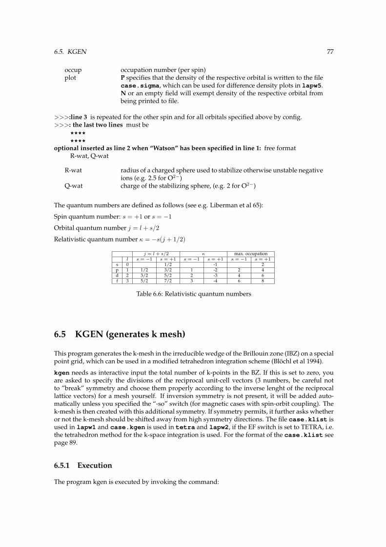
6.5. KGEN 77
occup occupation number (per spin)plot P specifies that the density of the respective orbital is written to the file
case.sigma, which can be used for difference density plots in lapw5.N or an empty field will exempt density of the respective orbital frombeing printed to file.
>>>:line 3 is repeated for the other spin and for all orbitals specified above by config.>>>: the last two lines must be
********
optional inserted as line 2 when “Watson” has been specified in line 1: free formatR-wat, Q-wat
R-wat radius of a charged sphere used to stabilize otherwise unstable negativeions (e.g. 2.5 for O2−)
Q-wat charge of the stabilizing sphere, (e.g. 2 for O2−)
The quantum numbers are defined as follows (see e.g. Liberman et al 65):
Spin quantum number: s = +1 or s = −1
Orbital quantum number j = l + s/2
Relativistic quantum number κ = −s(j + 1/2)
j = l + s/2 κ max. occupationl s = −1 s = +1 s = −1 s = +1 s = −1 s = +1
s 0 1/2 -1 2p 1 1/2 3/2 1 -2 2 4d 2 3/2 5/2 2 -3 4 6f 3 5/2 7/2 3 -4 6 8
Table 6.6: Relativistic quantum numbers
6.5 KGEN (generates k mesh)
This program generates the k-mesh in the irreducible wedge of the Brillouin zone (IBZ) on a specialpoint grid, which can be used in a modified tetrahedron integration scheme (Blochl et al 1994).
kgen needs as interactive input the total number of k-points in the BZ. If this is set to zero, youare asked to specify the divisions of the reciprocal unit-cell vectors (3 numbers, be careful notto ”break” symmetry and choose them properly according to the inverse lenght of the reciprocallattice vectors) for a mesh yourself. If inversion symmetry is not present, it will be added auto-matically unless you specified the “-so” switch (for magnetic cases with spin-orbit coupling). Thek-mesh is then created with this additional symmetry. If symmetry permits, it further asks whetheror not the k-mesh should be shifted away from high symmetry directions. The file case.klist isused in lapw1 and case.kgen is used in tetra and lapw2, if the EF switch is set to TETRA, i.e.the tetrahedron method for the k-space integration is used. For the format of the case.klist seepage 89.
6.5.1 Execution
The program kgen is executed by invoking the command:

78 CHAPTER 6. INITIALIZATION
kgen kgen.def or x kgen [-so]
With the switch -so it uses a file case.ksym (usually generated by symmetso) instead ofcase.struct and does not add inversion symmetry.
6.5.2 Dimensioning parameters
The following parameters are used in main.f, ord1.f (static arrays):
IDKP number of inequivalent k-points (like NKPT in other programs)NWX internal parameter, must be increased for very large k-meshesINDEXM internal parameter, must be increased for very large k-meshes
6.6 DSTART (superposition of atomic densities)
This program generates an initial crystalline charge density case.clmsum by a superposition ofatomic densities (case.rsp) generated with lstart. Information about LM values of the latticeharmonics representation and number of Fourier coefficients of the interstitial charge density aretaken from case.in1 and case.in2. In the case of a spin-polarized calculation it must also berun for the spin-up charge density case.clmup and spin-down charge density case.clmdn.
6.6.1 Execution
The program dstart is executed by invoking the command:
dstart dstart.def or x dstart [-up|dn -c -fft]
With the switch -fft dstart will terminate after case.in0 std has been created.
6.6.2 Dimensioning parameters
The following parameters are collected in file module.f, but usually need not to be changed:
NPT number of r-mesh points in atomic density (should be the same as in LSTART)LMAX2 max l in LM expansionNCOM number of LM terms in density

7 Programs for running an SCF cycle
Contents7.1 LAPW0 . . . . . . . . . . . . . . . . . . . . . . . . . . . . . . . . . . . . . . . . . . . 797.2 ORB . . . . . . . . . . . . . . . . . . . . . . . . . . . . . . . . . . . . . . . . . . . . . 827.3 LAPW1 . . . . . . . . . . . . . . . . . . . . . . . . . . . . . . . . . . . . . . . . . . . 867.4 LAPWSO . . . . . . . . . . . . . . . . . . . . . . . . . . . . . . . . . . . . . . . . . . 917.5 LAPW2 . . . . . . . . . . . . . . . . . . . . . . . . . . . . . . . . . . . . . . . . . . . 937.6 SUMPARA . . . . . . . . . . . . . . . . . . . . . . . . . . . . . . . . . . . . . . . . . 977.7 LAPWDM . . . . . . . . . . . . . . . . . . . . . . . . . . . . . . . . . . . . . . . . . 987.8 LCORE . . . . . . . . . . . . . . . . . . . . . . . . . . . . . . . . . . . . . . . . . . . 997.9 MIXER . . . . . . . . . . . . . . . . . . . . . . . . . . . . . . . . . . . . . . . . . . . 101
In sections 7.1-7.9 we describe the main programs to run an SCF cycle as illustrated in figure 4.1.
7.1 LAPW0 (generates potential)
lapw0 computes the total potential Vtot as the sum of the Coulomb Vc and the exchange-correlationpotential Vxc using the total electron (spin) density as input. It generates the spherical part (l=0)as case.vsp and the non-spherical part as case.vns. For spin-polarized systems, the spin-densities case.clmup and case.clmdn lead to two pairs of potential files. These files are called:case.vspup, case.vnsup and case.vspdn, case.vnsdn.
The Coulomb potential is calculated by the multipolar Fourier expansion introduced by Weinert(81). Utilizing the spatial partitioning of the unit cell and the dual representation of the charge den-sity [equ. 2.10], firstly the multipole moments inside the spheres are calculated (Q-sp). The Fourierseries of the charge density in the interstitial also represent SOME density inside the spheres, butcertainly NOT the correct density there. Nevertheless, the multipole moments of this artificialplane-wave density inside each sphere are also calculated (Q-pw). By subtracting Q-pw from Q-spone obtains pseudo-multipole moments Q. Next a new plane-wave series is generated which hastwo properties, namely zero density in the interstitial region and a charge distribution inside thespheres that reproduces the pseudo-multipole moments Q. This series is added to the original in-terstitial Fourier series for the density to form a new series which has two desirable properties: itsimultaneously represents the interstitial charge density AND it has the same multipole momentsinside the spheres as the actual density. Using this Fourier series the interstitial Coulomb potentialfollows immediately by dividing the Fourier coefficients by K2 (up to a constant).
Inside the spheres the Coulomb potential is obtained by a straightforward classical Green’s func-tion method for the solution of the boundary value problem.
The exchange-correlation potential is computed numerically on a grid. Inside the atomic spheres aleast squares procedure is used to reproduce the potential using a lattice harmonics representation
79
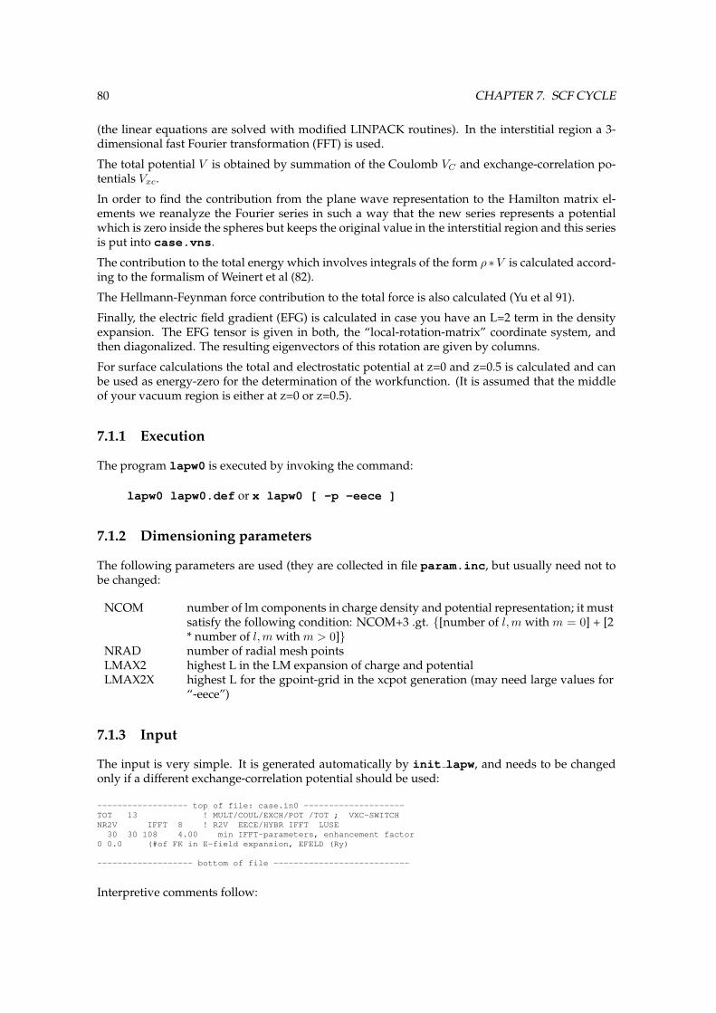
80 CHAPTER 7. SCF CYCLE
(the linear equations are solved with modified LINPACK routines). In the interstitial region a 3-dimensional fast Fourier transformation (FFT) is used.
The total potential V is obtained by summation of the Coulomb VC and exchange-correlation po-tentials Vxc.
In order to find the contribution from the plane wave representation to the Hamilton matrix el-ements we reanalyze the Fourier series in such a way that the new series represents a potentialwhich is zero inside the spheres but keeps the original value in the interstitial region and this seriesis put into case.vns.
The contribution to the total energy which involves integrals of the form ρ ∗V is calculated accord-ing to the formalism of Weinert et al (82).
The Hellmann-Feynman force contribution to the total force is also calculated (Yu et al 91).
Finally, the electric field gradient (EFG) is calculated in case you have an L=2 term in the densityexpansion. The EFG tensor is given in both, the “local-rotation-matrix” coordinate system, andthen diagonalized. The resulting eigenvectors of this rotation are given by columns.
For surface calculations the total and electrostatic potential at z=0 and z=0.5 is calculated and canbe used as energy-zero for the determination of the workfunction. (It is assumed that the middleof your vacuum region is either at z=0 or z=0.5).
7.1.1 Execution
The program lapw0 is executed by invoking the command:
lapw0 lapw0.def or x lapw0 [ -p -eece ]
7.1.2 Dimensioning parameters
The following parameters are used (they are collected in file param.inc, but usually need not tobe changed:
NCOM number of lm components in charge density and potential representation; it mustsatisfy the following condition: NCOM+3 .gt. [number of l,m with m = 0] + [2* number of l,m with m > 0]
NRAD number of radial mesh pointsLMAX2 highest L in the LM expansion of charge and potentialLMAX2X highest L for the gpoint-grid in the xcpot generation (may need large values for
“-eece”)
7.1.3 Input
The input is very simple. It is generated automatically by init lapw, and needs to be changedonly if a different exchange-correlation potential should be used:
------------------ top of file: case.in0 --------------------TOT 13 ! MULT/COUL/EXCH/POT /TOT ; VXC-SWITCHNR2V IFFT 8 ! R2V EECE/HYBR IFFT LUSE30 30 108 4.00 min IFFT-parameters, enhancement factor
0 0.0 (#of FK in E-field expansion, EFELD (Ry)
------------------- bottom of file ---------------------------
Interpretive comments follow:
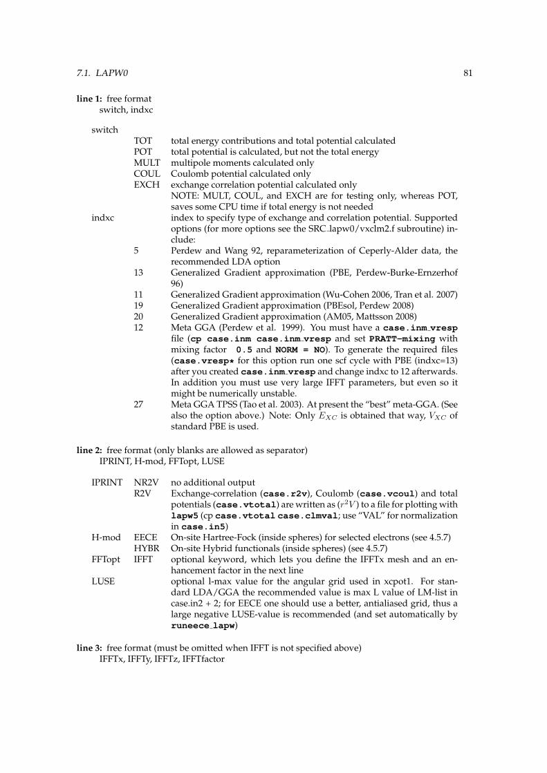
7.1. LAPW0 81
line 1: free formatswitch, indxc
switchTOT total energy contributions and total potential calculatedPOT total potential is calculated, but not the total energyMULT multipole moments calculated onlyCOUL Coulomb potential calculated onlyEXCH exchange correlation potential calculated only
NOTE: MULT, COUL, and EXCH are for testing only, whereas POT,saves some CPU time if total energy is not needed
indxc index to specify type of exchange and correlation potential. Supportedoptions (for more options see the SRC lapw0/vxclm2.f subroutine) in-clude:
5 Perdew and Wang 92, reparameterization of Ceperly-Alder data, therecommended LDA option
13 Generalized Gradient approximation (PBE, Perdew-Burke-Ernzerhof96)
11 Generalized Gradient approximation (Wu-Cohen 2006, Tran et al. 2007)19 Generalized Gradient approximation (PBEsol, Perdew 2008)20 Generalized Gradient approximation (AM05, Mattsson 2008)12 Meta GGA (Perdew et al. 1999). You must have a case.inm vresp
file (cp case.inm case.inm vresp and set PRATT-mixing withmixing factor 0.5 and NORM = NO). To generate the required files(case.vresp* for this option run one scf cycle with PBE (indxc=13)after you created case.inm vresp and change indxc to 12 afterwards.In addition you must use very large IFFT parameters, but even so itmight be numerically unstable.
27 Meta GGA TPSS (Tao et al. 2003). At present the “best” meta-GGA. (Seealso the option above.) Note: Only EXC is obtained that way, VXC ofstandard PBE is used.
line 2: free format (only blanks are allowed as separator)IPRINT, H-mod, FFTopt, LUSE
IPRINT NR2V no additional outputR2V Exchange-correlation (case.r2v), Coulomb (case.vcoul) and total
potentials (case.vtotal) are written as (r2V ) to a file for plotting withlapw5 (cp case.vtotal case.clmval; use “VAL” for normalizationin case.in5)
H-mod EECE On-site Hartree-Fock (inside spheres) for selected electrons (see 4.5.7)HYBR On-site Hybrid functionals (inside spheres) (see 4.5.7)
FFTopt IFFT optional keyword, which lets you define the IFFTx mesh and an en-hancement factor in the next line
LUSE optional l-max value for the angular grid used in xcpot1. For stan-dard LDA/GGA the recommended value is max L value of LM-list incase.in2 + 2; for EECE one should use a better, antialiased grid, thus alarge negative LUSE-value is recommended (and set automatically byruneece lapw)
line 3: free format (must be omitted when IFFT is not specified above)IFFTx, IFFTy, IFFTz, IFFTfactor

82 CHAPTER 7. SCF CYCLE
IFFTx,y,z FFT-mesh parameters in x,y,z directions for the calculation of theXC-potential in the interstitial region. Usually set automatically ininit lapw (dstart). The ratio of the 3 numbers should be indirect pro-portional to the lattice parameters. (-1 -1 -1 determines these numbersautomatically and takes only IFFTfactor into account)
IFFTfactor Multiplicative factor to the IFFT grid specified above. It needs to beenlarged for highly accurate GGA or meta-GGA calculations as well asfor systems with H atoms with small spheres.
The following line is optional and can be omitted. It is used to introduce an electric field viaa zig-zag potential (see J.Stahn et al. 2001):
line 4: free formatIFIELD, EFIELD, WFIELD
IFIELD number of Fourier coefficients to model the zig-zag potential. Typicallyuse IEFIELD=30; -999 lists available modes (form) of fields, and thesemodes can be specified by mode=IEFIELD/1000. (default: mode=0)
EFIELD value (amplitude) of the electric field. The electric field (in Ry/bohr)corresponds to EFIELD/c, where c is your c lattice parameter.
WFIELD optional value for lambda (see output of IEFIELD=-999).
7.2 ORB (Calculate orbital dependent potentials)
This program was contributed by:
P.NovakInst. of Physics, Acad.Science, Prague, Czeck Republicemail: [email protected]
Please make comments or report problems with this program to the WIEN-mailinglist. If necessary,
we will communicate the problem to the authors.
orb calculates the orbital dependent potentials, i.e. potentials which are nonzero in the atomicspheres only and depend on the orbital state numbers l,m. In the present version the potential isassumed to be independent of the radius vector and needs the density matrix calculated in lapwdm.Four different potentials are implemented in this package:
I LDA+U. There are three variants of this method, two of them are discussed in Novak et al.2001
1. LDA+U(SIC) - introduced by Anisimov et al. 1993, with an approximate correction forthe self-interaction correction. This is probably best suited for strongly correlated sys-tems and for a full potential method we recommend to use an “effective” Ueff = U − J ;setting J = 0.
2. LDA+U(AMF) - introduced by Czyzyk and Sawatzky 1994 as ’Around the Mean Field’method. (In Novak et al. 2001 it is denoted as LDA+U(DFT)). This version is (probably)more suitable for metallic or less strongly correlated systems.
3. LDA+U(HMF) - in addition the Hubbard model in the mean field approximation, asintroduced by Anisimov et al. 1991 is also implemented. Note, however, that it is to beused with the LDA (not LSDA) exchange-correlation potential in spin polarized calcu-lations!

7.2. ORB 83
All variants are implemented in the rotationally invariant way (Liechtenstein et al. 1995). IfLDA+U is used in an unrestricted, general way, it introduces an orbital field in the calcu-lation (in analogy to the exchange field in spin-polarized calculations, but it interacts withthe orbital, instead of spin momentum). The presence of such an orbital field may lower thesymmetry. In particular the complex version of LAPW1 must be used. Care is needed whendealing with the LDA+U orbital field. It may be quite large, and without specifying its direc-tion it may fluctuate, leading to oscillations of scf procedure or/and to false solutions. It istherefore necessary to use it in combination with the spin-orbit coupling, preferably runningfirst LSDA+(s-o) and then slowly switching on the LDA+U orbital field. If the LDA+U orbitalpolarization is not needed, it is sufficient to run real version of LAPW1, which then automat-ically puts the orbital field equal to zero. For systems without the center of inversion, whenLAPW1 must be complex, an extra averaging of the LDA+U potential is necessary.
I Orbital polarization. The additional potential has the form (Brooks 1985, Eriksson et al. 1989):VOP = cOP < Lz > lz (7.1)
where cOP is the orbital polarization parameter, < Lz > is projection of the orbital momen-tum on the magnetization direction and lz is single electron orbital momentum component zparallel to ~M .
I Exact exchange and Hybrid methods: see Tran et al. 2006 and 4.5.7I Interaction with the external magnetic field. In this case the additional potential has a simple
form:VBext = µB
~Bext(~l + 2~s). (7.2)The interaction with the electronic spin is taken into account by shifting the spin up and spindown exchange correlation potentials in LAPW0 by the energy +µBBext − µBBext, respec-tively. The interaction of Bext with spin could be as well calculated using the ’Fixed spinmoment’ method. For an interaction with the orbital momentum it is necessary to specify theatoms and angular momentum numbers for which this interaction will be considered. Cau-tion is needed when considering interaction of the orbital momentum with Bext in metallicor metallic-like systems. For the analysis see the paper by Hirst 1997
In all cases the resulting potential for a given atom and orbital number l is a Hermitian, (2l +1)x(2l + 1) matrix. In general this matrix is complex, but in special cases it may be real.
For more information see also section 4.5.6.
7.2.1 Execution
The program orb is executed by invoking the command:
x orb [ -up/-dn/-du ] or orb up/dnorb.def
7.2.2 Dimensioning parameters
The following parameters are used (collected in file param.inc):
LABC highest l+1 value of orbital dependent potentialsNRAD number of radial mesh points
7.2.3 Input
Since this program can handle three different cases, examples and descriptions for all cases aregiven below:

84 CHAPTER 7. SCF CYCLE
Input for all potentials
line 1: free formatnmod,natorb,ipr
nmod defines the type of potential 1...LDA+U, 2...OP, 3...Bext
natorb number of atoms for which orbital potential Vorb is calculatedipr printing option, the larger ipr, the longer the output
line 2: (A5,f8.2)mixmod,amix
mixmod PRATT or BROYD (should not be changed, see MIXER for more infor-mation)
amix coefficient for the Pratt mixing of Vorb
This option is now only used for testing. The mixing should be set toPRATT, 1.0
line 3: free formatiatom(i),nlorb(i),(lorb(li,i),li=1,nlorb(i))
iatom index of atom in struct filenlorb number of orbital moments for which Vorb shall be appliedlorb orbital numbers (repeated nlorb-times)
3rd line repeated natorb-times
Input for LDA+U (nmod=1)
line 4: free format
nsic defines ’double counting correction’nsic=0 ’AMF method’ (Czyzyk et al. 1994)nsic=1 ’SIC method’ (Anisimov et al. 1993, Liechtenstein et al. 1995)nsic=2 ’HMF method’ (Anisimov et al. 1991)
line 5: free format
U(li,i),J(li,i)
Coulomb and exchange parameters, U and J, for LDA+U in Ry for atomtype i and orbital number li. We recommend to use Ueff only.
5th line repeated natorb-times, for each natorb repeated nlorb-times
Example of the input file for NiO (LDA+U included for two inequivalent Ni atoms that have in-dexes 1 and 2 in the structure file):
1 2 0 nmod, natorb, iprPRATT,1.0 mixmod, amix1 1 2 iatom nlorb, lorb2 1 2 iatom nlorb, lorb1 nsic (LDA+U(SIC) used)0.52 0.0 U J0.52 0.0 U J

7.2. ORB 85
Input for Orbital Polarization (nmod=2)
line 4: (free format)
nmodop defines mode of ’OP’1 average Lz taken separately for spin up, spin down0 average Lz is the sum for spin up and spin down
line 5: (free format)
Ncalc(i)1 Orb.pol. parameters are calculated ab-initio0 Orb.pol. parameters are read from input
this line is repeated natorb-timesline 6: (free format) (only if Ncalc=0, then repeated nlorb-times)
pop(li,i) OP parameter in Ry
line 7: (free format)xms(1), xms(2), xms(3)
direction of magnetization expressed in terms of lattice vectors
Example of the input file for NiO (total < Lz > used in (1), OP parameters calculated ab-initio, ~Malong [001]):
2 2 0 nmod, natorb, iprPRATT, 1.0 mixmod, amix1 1 2 iatom nlorb, lorb2 1 2 iatom nlorb, lorb0 nmodop1 Ncalc1 Ncalc0. 0. 1. direction of M in terms of lattice vectors
Input for interaction with Bext (nmod=3)
line 4: (free format)
Bext external field in Tesla
line 5: (free format)xms(1), xms(2), xms(3)
direction of magnetization expressed in terms of lattice vectors
Example of the input file for NiO, (Bext= 4 T, along [001]):
3 2 0 nmod, natorb, iprPRATT, 1.0 mixmod, amix1 1 2 iatom nlorb, lorb2 1 2 iatom nlorb, lorb4. Bext in T

86 CHAPTER 7. SCF CYCLE
0. 0. 1. direction of Bext in terms of lattice vectors
7.3 LAPW1 (generates eigenvalues and eigenvectors)
lapw1 sets up the Hamiltonian and the overlap matrix (Koelling and Arbman 75) and finds bydiagonalization eigenvalues and eigenvectors which are written to case.vector. Besides thestandard LAPW basis set, also the APW+lo method (see Sjostedt et al 2000, Madsen et al. 2001) issupported and the basis sets can be mixed for maximal efficiency. If the file case.vns exists (i.e.non-spherical terms in the potential), a full-potential calculation is performed.
For structures without inversion symmetry, where the hamilton and overlap matrix elements arecomplex numbers, the corresponding program version lapw1c must be used in connection withlapw2c.
Since usually the diagonalization is the most time consuming part of the calculations, two optionsexist here. In WIEN2k we include highly optimized modifications of LAPACK routines. We call allthese routines “full diagonalization”, but we also provide an option to do an “iterative diagonal-ization” using a new preconditioning of a block-Davidson method (see Singh 89 and Hofstatter etal. 08). This scheme starts from an old eigenvector (previous scf-iteration), and produces approx-imate (but usually still highly accurate) eigenvalues/vectors. Depending on the ratio of matrixsize to number of eigenvalues (restrict them to relevant, i.e. occupied states) a significant speedupcompared to LAPACK can be reached. Iterative diagonalization is activated with the -it switchin x lapw1 -it or run lapw -it.
Parallel execution (fine grain and on the k-point level) is also possible and is described in detail inSec. 5.5.
The switch -nohns skips the calculation of the nonspherical matrix elements inside the sphere.This may be used to save computer time during the first scf cycles.
7.3.1 Execution
The program lapw1 is executed by invoking the command:
x lapw1 [-c -up|dn -it -p -nohns -orb -band -nmat only] or
lapw1 lapw1.def or lapw1c lapw1.def
In cases without inversion symmetry, the default input filename is case.in1c. For 2-window (notrecommended) semi-core calculations the lapw1s.def file uses a case.in1s file and creates thefiles case.output1s and case.vectors. For the spin-polarized case lapw1 is called twice withuplapw1.def and dnlapw1.def. To all relevant files the keywords “up“ or “dn“ are appended(see the fcc Ni test case in the WIEN2k package).
7.3.2 Dimensioning parameters
The following parameters (collected in file param.inc r or param.inc c) are used:
LMAX highest l+1 in basis function inside sphere (consistent with input in case.in1)LMMX number of LM terms in potential (should be at least NCOM-1)LOMAX highest l for local orbital basis (consistent with input in case.in1)NGAU number of Gaunt coefficients for the non-spherical contributions to the matrix
elementsNMATMAX maximum size of H,S-matrix (defines size of program, should be chosen accord-
ing to the memory of your hardware, see chapter 11.2.2!)NRAD number of radial mesh pointsNSLMAX highest l+1 in basis functions for non-muffin-tin matrix elements (consistent with
input in case.in1).If set larger than 5, parameter MAXDIM (modules.F) and LO-MAX=8, P(10,10) (gaunt2.f) must also be increased.
7.3. LAPW1 87
NSYM order of point groupNUME maximum number of energy eigenvalues per k-pointNVEC1 defines the largest triple of integers which define reciprocalNVEC2 K-vectors when multiplied with the reciprocal Bravais matrixNVEC3NLOAT max number of LOs for one l-quantum number
7.3.3 Input
Below a sample input is shown for TiO2 (rutile), one of the test cases provided in the WIEN2kpackage. The input file is written automatically by LSTART, but was modified to set APW only forTi-3d and O-2p orbitals. In addition UNIT was changed to 5 and k-points where inserted by handfor bandstructure plotting.
------------------ top of file: case.in1 --------------------WFFIL (WFPRI,WFFIL,SUPWF ; wave fct. print,file,suppress7.500 10 4 (R-mt*K-max; MAX l, max l for hns )0.30 5 0 (global energy parameter E(l), with 5 other choices, LAPW)
0 -3.00 0.020 CONT 0 ENERGY PARAMETER for s, LAPW0 0.30 0.000 CONT 0 ENERGY PARAMETER for s-local orbital, LAPW-LO1 -1.90 0.020 CONT 0 ENERGY PARAMETER for p LAPW1 0.30 0.000 CONT 0 ENERGY PARAMETER for p-local orbitals LAPW-LO2 0.20 0.020 CONT 1 APW0.20 3 0 (global energy parameter E(l), with 1 other choice, LAPW)
0 -0.90 0.020 STOP 0 LAPW0 0.30 0.000 CONT 0 LAPW-LO1 0.30 0.000 CONT 1 APW
K-VECTORS FROM UNIT:5 -9.0 2.0 60 emin/emax/nband1.d-15 spro_limit for it.diag.GAMMA 0 0 0 2 1.00
0 0 1 10 2.000 0 2 10 2.000 0 3 10 2.000 0 4 10 2.00
Z 0 0 5 10 1.00END------------------- bottom of file ------------------------
Interpretive comments follow:
line 1: format(A5)switch
WFFIL standard option, writes wave functions to file case.vector (neededin lapw2)
SUPWF suppresses wave function calculation (faster for testing eigenvaluesonly)
WFPRI prints eigenvectors to case.output1 and writes case.vector (pro-duces long outputs!)
line 2: free formatrkmax, lmax, lnsmax

88 CHAPTER 7. SCF CYCLE
rkmax Rmt ∗ Kmax determines matrix size (convergence), where Kmax is theplane wave cut-off, Rmt is the smallest of all atomic sphere radii. Usu-ally this value should be between 5 and 9 (APW+lo) or 6 - 10. (LAPW-basis) (K2
max would be the plane wave cut-off parameter in Ry usedin pseudopotential calculations.) Note that d (f) wavefunctions con-verge slower than s and p. For systems including hydrogen with shortbondlength and thus a very small Rmt (e.g. 0.7 a.u.), RKmax = 3 mightalready be reasonable, but convergence must be checked for a new typeof system.Note, that the actual matrix size is written on case.scf1. It is determinedby whatever is smaller, the plane wave cut-off (specified with RKmax)or the maximum matrix dimension NMATMAX, (see previous section).
lmax maximum l value for partial waves used inside atomic spheres (shouldbe between 8 and 12)
lnsmax maximum l value for partial waves used in the computation of non-muffin-tin matrix elements (lnsmax=4 is quite good)
line 3: free formatEtrial, ndiff, Napw
Etrial default energy used for all El to obtain ul(r, El) as regular solution ofthe radial Schrodinger equation [used in equ.2.4,2.7] (see figure 7.1).
ndiff number of exceptions (specified in the next ndiff lines)Napw 0 ... use LAPW basis, 1 ... use APW-basis for all “global” l values of this
atom. We recommend to use LAPW here.
line 4: format(I2,2F10.5,A4)l, El, de, switch, NAPWL
l l of partial waveEl El for L=lde energy increment
de=0: this E(l) overwrites the default energy (from line 3)de6= 0: a search for a resonance energy using this increment is done. Theradial function ul(r, E) up to the muffin-tin radius RMT varies with theenergy. A typical case is schematically shown in Fig. 7.1.At the bottom of the energy bands u has a zero slope (bonding state),but it has a zero value (antibonding state) at the top of the bands. Onecan search up and down in energy starting with El using the incrementde to find where ul(RMT , E) changes sign in value to determine Etop
and in slope to specify Ebottom. If both are found El is taken as thearithmetic mean and replaces the trial energy. Otherwise El keeps thespecified value. For Etop and Ebottom bounds of +1 and -10 Ry are de-fined respectively, and if they are not found, they remain at the initialvalue set to -200.
switch used only if de.ne.0CONT calculation continues, even if either Etop or Ebottom are not foundSTOP calculation stops if not both Etop and Ebottom are found (especially use-
ful for semi-core states)NAPWL 0 ... use LAPW basis, 1 ... use APW-basis for this l value of this atom. We
recommend to use APW+lo when the corresponding wavefunction is“localized” and thus difficult to converge with standard LAPW (like 3dfunctions) and/or when the respective atomic sphere is small comparedto the other spheres in the unit cell.
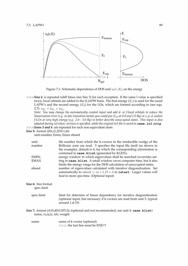
7.3. LAPW1 89
l
Etop
Ebottom
Ebottom
El
Etop
u (r,E)l
RMT
E
DOSr
E
Figure 7.1: Schematic dependence of DOS and ul(r, El) on the energy
>>>:line 4 is repeated ndiff times (see line 3) for each exception. If the same l value is specifiedtwice, local orbitals are added to the (L)APW basis. The first energy (E1) is used for the usualLAPW’s and the second energy (E2) for the LOs, which are formed according to (see equ.2.7): uE1 + uE1 + uE2 .Note: You may change the automatically created input and add d- or f-local orbitals to reduce thelinearization error (e.g. in late transition metals you could put E3d at 0.0 and 1.0 Ry) or s, p, d, and/orf-LOs at very high energy (e.g. 2.0 - 3.0 Ry) to better describe unoccupied states. This input is alsoadapted during scf when -in1new is specified, while the original in1 file is saved in case.in1 orig.
>>>:lines 3 and 4 are repeated for each non equivalent atomline 5: format (20x,i1,2f10.1,i6)
unit-number, Emin, Emax nband
unit-number
file number from which the k-vectors in the irreducible wedge of theBrillouin zone are read. 5 specifies the input file itself (as shown inthe example), default is 4, for which the corresponding information iscontained in case.klist (generated by KGEN).
EMIN,EMAX
energy window in which eigenvalues shall be searched (overrides set-ting in case.klist. A small window saves computer time, but it alsolimits the energy range for the DOS calculation of unoccupied states.
nband number of eigenvalues calculated with iterative diagonalization. Setautomatically to nband = ne ∗ 1.15 + 5 in lstart. Larger values willlead to more cpu-time. (Optional input)
line 6: free formatspro limit
spro limit limit for detection of linear dependency for iterative diagonalization(optional input, but necessary if k-vectors are read from unit 5, typicalaround 1.d-15)
line 7: format (A10,4I10,3F5.2); (optional and not recommended, use unit 4: case.klist)name, ix,iy,iz, idv, weight
name name of k-vector (optional)>>>: the last line must be END !!

90 CHAPTER 7. SCF CYCLE
ix,iy,iz,idv
defines the k-vector, where x= ix/idv etc. We use carthesian coordi-nates in units of 2π/a, 2π/b, 2π/c for P,C,F and B cubic, tetragonaland orthorhombic lattices, but internal coordinates for H and mono-clinic/triclinic lattices
weight of k-vector (order of group of k)
>>>: line 7 is repeated for each k-vector in the IBZ. The utility program kgen (see section 6.5)provides a list of such vectors (on a tetrahedral mesh) in case.klist.
>>>: the last line must be END

7.4. LAPWSO 91
7.4 LAPWSO (adds spin orbit coupling)
lapwso includes spin-orbit (SO) coupling in a second-variational procedure and computes eigen-values and eigenvectors (stored in case.vectorso) using the scalar-relativistic wavefunctionsfrom lapw1. For reference see Singh 94 and Novak 97. The SO coupling must be small, as it isdiagonalized in the space of the scalar relativistic eigenstates. For large spin orbit effects it mightbe necessary to include many more eigenstates from lapw1 by increasing EMAX in case.in1 (upto 10 Ry!). We also provide an additional basisfunction, namely an LO with a p1/2 radial wave-function, which improves the basis and removes to a large degree the dependency of the resultson EMAX and RMT (see Kunes et al. 2001). SO is considered only within the atomic spheres andthus the results may depend to some extent on the choice of atomic spheres radii. The nonsphericalpotential is neglected when calculating dV
dr . Orbital dependend potentials (LDA+U, EECE or OP)can be added to the hamiltonian in a cheap and simple way.
In spin-polarized calculations the presence of spin-orbit coupling may reduce symmetry and evensplit equivalent atoms into non-equivalent ones. It is then necessary to consider a larger part ofthe Brillouin zone and the input for lapw2 should also be modified since the potential has lowersymmetry than in the non-relativistic case. The following inputs may change:
I case.structI case.klistI case.kgenI case.in2cI case.in1
We recommend to use initso (see Sec.5.2.16) which helps you together with symmetso (seeSec.9.1) to setup spinorbit calculations.
Note: SO eigenvectors are complex and thus lapw2c must be used in a selfconsistent calculation.
7.4.1 Execution
The program lapwso is executed by invoking the command:
x lapwso [ -up -p -c -orb] orlapwso lapwso.def
where here -up indicates a spin-polarized calculation (no “-dn” is needed, since spin-orbit will mixspin-up and dn states in one calculation).
7.4.2 Dimensioning parameters
The following parameters are used (collected in file param.inc):
FLMAX constant = 3LMAX highest l of wave function inside sphere (consistent with lapw1)LABC highest l of wave function inside sphere where SO is consideredLOMAX max l for local orbital basisNRAD number of radial mesh pointsNLOAT number of local orbitals

92 CHAPTER 7. SCF CYCLE
7.4.3 Input
A sample input for lapwso is given below. It will be generated automatically by initso
------------------ top of file: case.inso --------------------WFFIL4 0 0 llmax,ipr,kpot-10.0000 1.5000 Emin, Emax
0 0 1 h,k,l (direction of magnetization)2 number of atoms with RLO
1 -3.5 0.005 STOP atom-number, E-param for RLO3 -4.5 0.005 STOP atom-number, E-param for RLO1 2 number of atoms without SO, atomnumbers
------------------- bottom of file ------------------------
Interpretive comments on this file are as follows:
line 1: format(A5)switch
WFFIL wavefunctions will also be calculated for scf-calculation. Otherwiseonly eigenvalues are calculated.
line 2: free formatLLMAX, IPR, KPOT
LLMAX maximum l for wavefunctionsIPR print switch, larger numbers give additional output.KPOT 0 V(dn) potential is used for < dn|V |dn > elements, V(up) for
< up|V |up > and [V(dn)+V(up)]/2 for < up|V |dn >.1 averaged potential used for all matrix elements.
line 3: free formatEmin, Emax
Emin minimum energy for which the output eigenvectors and eigenenergieswill be printed (Ry)
Emax maximum energy
line 4: free format
h,k,l vector describing the direction of magnetization. For R lattice use h,k,lin rhombohedral coordinates (not in hexagonal)
line 5: free format
nlr number of atoms for which a p1/2 LO should be added
line 6: free formatnlri, El, de, switch
nlri atom-number for which RLO should be addedEl El for L=lde energy increment (see lapw1)switch used only if de.ne.0
CONT calculation continues, even if either Etop or Ebottom are not found

7.5. LAPW2 93
STOP calculation stops if not both Etop and Ebottom are found (especially use-ful for semi-core states)
>>>: line 6 must be repeated “nlr” times (or should be omitted if nlr=0).line 7: free format
noff, (iatoff(i),i=1,noff)
noff number of atoms for which SO is switched off (for “light” elements,saves time)
iatoff atom-numbers
7.5 LAPW2 (generates valence charge density expansions)
lapw2 uses the files case.energy and case.vector and computes the Fermi-energy (for asemiconductorEF is set to the valence band maximum) and the expansions of the electronic chargedensities in a representation according to eqn. 2.10 for each occupied state and each k-vector;then the corresponding (partial) charges inside the atomic spheres are obtained by integration. Inaddition “Pulay-corrections“ to the forces at the nuclei are calculated here. For systems withoutinversion symmetry you have to use the program lapw2c (in connection with lapw1c).
The partial charges for each state (energy eigenvalue) and each k-vector can be written to filescase.help031, case.help032 etc., where the last digit gives the atomic index of inequiva-lent atoms (switch -help files). Optionally these partial charges are also written to case.qtl(switch -qtl). For meta-GGA calculations energy densities are written to case.vrepval(switch-vresp).
In order to get partial charges for bandstructure plots, use -band, which sets the “QTL option anduses “ROOT” in case.in2. Several other switches change the input file case.in2 temporarelyand are described there.
7.5.1 Execution
The program lapw2 is executed by invoking the command:
x lapw2 [-c -up|dn -p -so -qtl -fermi -efg -band -eece -vresp-help files -emin X -all X Y] orlapw2 lapw2.def [proc#] or lapw2c lapw2.def [proc#]
where proc# is the i-th processor number in case of parallel execution (see Fig. 5.2). The -so switchsets -c automatically.
For complex calculations case.in2c is used. For a spin-polarized case see the fcc Ni test case inthe WIEN2k package.
7.5.2 Dimensioning parameters
The following parameters are used (collected in file modules.F):
IBLOCK Blocking parameter (32-255) in l2main.F, optimize for best performanceLMAX2 highest l in wave function inside sphere (smaller than in lapw1, at present must
be .le. 8)LOMAX max l for local orbital basis

94 CHAPTER 7. SCF CYCLE
NCOM number of LM terms in densityNGAU max. number of Gaunt numbersNRAD number of radial mesh points
7.5.3 Input
A sample input for lapw2 is listed below, it is generated automatically by the programs lstartand symmetry.
------------------ top of file: case.in2 --------------------TOT (TOT,FOR,QTL,EFG)-1.2 32.000 0.5 0.05 (EMIN, # of electrons,ESEPERMIN, ESEPER0 )TETRA 0.0 (EF-method (ROOT,TEMP,GAUSS,TETRA,ALL),value)0 0 2 0 2 2 4 0 4 2 4 40 0 1 0 2 0 2 2 3 0 3 2 4 0 4 2 4 4
14.0 (GMAX)FILE (NOFILE, optional)------------------- bottom of file ------------------------
Interpretive comments on this file are as follows:
line 1: format(2A5)switch, EECE
switch TOT total valence charge density expansion inside and outside spheresFOR same as TOT, but in addition a “Pulay” force contribution is calculated
(this option costs extra computing time and thus should be performedonly at the final scf cycles, see run lapw script in sec. 5.1.3)
QTL partial charges only (generates file case.qtl for DOS calculations), setautomatically by switch -qtl
EFG computes decomposition of electric field gradient (EFG), contributionsfrom inside spheres (the total EFG is computed in lapw0), set automat-ically by switch -efg.
ALM this generates two files, case.radwf and case.almblm, where theradial wavefunctions and the Alm, Blm, Clm coefficients of the wave-function inside spheres are listed. The file case.almblm can get verybig.
CLM CLM charge density coefficients onlyFERMI Fermi energy only, this produces weight files for parallel execution
and for the optics and lapwdm package, set automatically by switch-fermi.
>>>: TOT and FOR are the standard options, QTL is used for density of states(or energy bandstructure) calculations, EFG for analysis, while FOURI,CLM are for testing only.
EECE if set to “EECE”, calculates the density for specified atoms and angu-lar momentum only. Used for exact-exchange or hybrid-calculations,usually set automatically by runsp lapw -eece
line 2: free formatemin, ne, esepermin, eseper0
emin lower energy cut-off for defining the range of occupied states, can beset termporarely to “X” by switch -emin X or -all X Y
ne number of electrons (per unit cell) in that energy range

7.5. LAPW2 95
esepermin LAPW2 tries to find the “mean” energies for each l channel, for both thevalence and the semicore states. To define “valence” and “semicore” itstarts at (EF - “esepermin”) and searches for a “gap” with a width ofat least “eseper0” and defines this as separation energy of valence andsemicore
eseper0 minimum gap width (see above). The values esepermin and eseper0will only influence results if the option -in1new is used
line 3: format(a5,f10.5)efmod, eval
efmod determines how EF is determinedROOT EF is calculated and k space integration is done by root sampling (this
can be used for insulators, but for metals poor convergence is found)TEMP EF is calculated where each eigenvalue is temperature broadened using
a Fermi function with a broadening parameter of eval Ry. The totalenergy is corrected corresponding to T=0K. (e.g. eval=0.002 gives goodtotal energy convergence, but has no “physical“ justification)
TEMPS EF is calculated where each eigenvalue is temperature broadened usinga Fermi function with a broadening parameter of eval Ry. The totalenergy is corrected by -TS corresponding to the temperature specifiedby eval (e.g. eval=0.002 corresponds to about 40 C)
GAUSS EF is calculated as above but a Gaussian smearing method is used witha width of eval Ry. (e.g. eval=0.002 gives good total energy conver-gence, but has no “physical“ justification).
TETRA EF is calculated and k space integration is done by the modified (if evalis .eq. 0) or standard (eval .ge. 100) tetrahedron-method (Blochl 94).This “standard” scheme is recommended for optic. In this case thefile case.kgen, consistent with the k-mesh used in lapw1, must beprovided (see Sec. 7.3). This is the recommended option although con-vergence may be slower than with Gauss- or temperature-smearing.
ALL All states up to eval are used. This can be used to generate charge den-sities in a specified energy interval, can be set termporarely by switch-all X Y.
eval when efmod is set to TEMP or GAUSS, eval specifies the width of thebroadening (in Ry), if efmod is set to ALL, eval specifies the upper limitof the energy window (can be set termporarely by switch -all X Y),if efmod is set to TETRA, eval .ge. 100 specifies the use of the stan-dard tetrahedron method instead of the modified one (see above). Bydefault, TETRA will average over partially occupied degenerate statesat EF with a degeneracy criterium D = 1.d-6. You can modify this bysetting eval equal to your desired D (or 100+D).
optional line 3a: free format (ONLY when EECE is set)
nat rho number of atoms for which a specific density should be calculated
optional line 3b: free format (ONLY when EECE is set)jatom rho, l rho
jatom rho index of atom for which a specific density should be calculatedl rho angular momentum l-value for which a specific density should be cal-
culated

96 CHAPTER 7. SCF CYCLE
>>>line 3b: must be repeated nat rho timesline 4: format (121(I3,I2))
L,M LM values of lattice harmonics expansion (equ. 2.10), defined accord-ing to the point symmetry of the corresponding atom; generated inSYMMETRY, MUST be consistent with the local rotation matrix definedin case.struct (details can be found in Kara and Kurki-Suonio 81).CAUTION: additional LM terms which do not belong to the lattice har-monics will in general not vanish and thus such terms must be omitted.Automatic termination of the lm series occurs when a second 0,0 pairappears within the list. When you change the l,m list during an SCFcalculation the Broyden-Mixing is restarted in MIXER.
>>>line 4: must be repeated for each inequivalent atom
Symmetry LM combinations23 0 0, 4 0, 4 4, 6 0, 6 4,-3 2, 6 2, 6 6,-7 2,-7 6, 8 0, 8 4, 8 8,-9 2,-9 6,-9 4,-9 8,10 0, 10 4,10 8, 10 2, 10 6, 10 10M3 0 0, 4 0, 4 4, 6 0, 6 4, 6 2, 6 6, 8 0, 8 4, 8 8,10 0, 10 4,10 8, 10 2, 10 6, 10 10432 0 0, 4 0, 4 4, 6 0, 6 4, 8 0, 8 4, 8 8,-9 4,-9 8,10 0, 10 4,10 8-43M 0 0, 4 0, 4 4, 6 0, 6 4,-3 2,-7 2,-7 6, 8 0, 8 4, 8 8,-9 2,-9 6,10 0, 10 4,10 8M3M 0 0, 4 0, 4 4, 6 0, 6 4, 8 0, 8 4, 8 8,10 0, 10 4,10 8
Table 7.41: LM combinations of “Cubic groups” (3‖(111)) direction, requires “positive atomic in-dex” in case.struct. Terms that should be combined (Kara and Kurki-Suonio 81) must follow oneanother.
Symmetry Coordinate axes Indices of Y±LM crystal system1 any ALL (±l,m) triclinic-1 any (±2l,m)2 2‖ z (±l,2m) monoclinicM m⊥z (±l,l-2m)2/M 2‖z, m⊥z (±2l,2m)222 2‖z, 2‖y, (2‖x) (+2l,2m), (-2l+1,2m) orthorhombicMM2 2‖z, m⊥y, (2⊥x) (+l,2m)MMM 2⊥z, m⊥y, 2⊥x (+2l,2m)4 4‖z (±l,4m) tetragonal-4 -4‖z (±2l,4m), (±2l+1,4m+2)4/M 4‖z, m⊥z (±2l,4m)422 4‖z, 2‖y, (2‖x) (+2l,4m), (-2l+1,4m)4MM 4‖z, m⊥y, (2⊥x) (+l,4m)-42M -4‖z, 2‖x (m=xy→yx) (+2l,4m), (-2l+1,4m+2)4MMM 4‖z, m⊥z, m⊥x (+2l,4m)3 3‖z (±l,3m) rhombohedral-3 -3‖z (±2l,3m)32 3‖z, 2‖y (+2l,3m), (-2l+1,3m)3M 3‖z, m⊥y (+l,3m)-3M -3‖z, m⊥y (+2l,3m)6 6‖z (±l,6m) hexagonal-6 -6‖z (+2l,6m), (±2l+1,6m+3)6/M 6‖z, m⊥z (±2l,6m)622 6‖z, 2‖y, (2‖x) (+2l,6m), (-2l+1,6m)6MM 6‖z, m‖y, (m⊥x) (+l,6m)-62M -6‖z, m⊥y, (2‖x) (+2l,6m), (+2l+1,6m+3)6MMM 6‖z, m⊥z, m⊥y, (m⊥x) (+2l,6m)
Table 7.42: LM combination and local coordinate system of “non-cubic groups” (requires “negativeatomic index” in case.struct)
line 5: free format

7.6. SUMPARA 97
GMAX max. G (magnitude of largest vector) in charge density Fourier expan-sion. For systems with short H bonds larger values (e.g. GMAX upto 25) could be necessary. Calculations using GGA (potential option13 or 14 in case.in0) should also employ a larger GMAX value (e.g.14), since the gradients are calculated numerically on a mesh deter-mined by GMAX. When you change GMAX during an scf calculationthe Broyden-Mixing is restarted in mixer.
line 6: A4
reclist FILE writes list of K-vectors into file case.recprlist or reuses this list ifthe file exists. The saved list will be recalculated whenever GMAX, or alattice parameter has been changed.
NOFILE always calculate new list of K-vectors
7.6 SUMPARA (summation of files from parallel execution)
sumpara is a small program which (in parallel execution of WIEN2k) sums up the densities(case.clmval *) and quantities from the case.scf2 * files of the different parallel runs.
7.6.1 Execution
The program sumpara is executed by invoking the 2 commands as follows:
x sumpara -d [-up/-dn/-du] and thensumpara sumpara.def # of proc
where # of proc is the numbers of parallel processors used. It is usually called automaticallyfrom lapw2para or x lapw2 -p.
7.6.2 Dimensioning parameters
The following parameters are listend in file param.inc, but usually they need not to be modified:
NCOM number of LM terms in densityNRAD number of radial mesh pointsNSYM order of point group

98 CHAPTER 7. SCF CYCLE
7.7 LAPWDM (calculate density matrix)
This program was contributed by:
J.Kunes and P.NovakInst. of Physics, Acad.Science, Prague, Czeck Republicemail: [email protected]
Please make comments or report problems with this program to the WIEN-mailinglist. If necessary,
we will communicate the problem to the authors.
lapwdm calculates the density matrix needed for the orbital dependent potentials generated in orb.Optionally it also provides orbital moments, orbital and dipolar contributions to the hyperfine field(only for the specified atoms AND orbitals). It calculates the average value of the operator X whichbehaves in the same way as the spin-orbit coupling operator: it must be nonzero only within theatomic spheres and can be written as a product of two operators - radial and angular:
X = Xr(r) ∗Xls(~l, ~s)
Xr(r) and Xls(~l, ~s) are determined by RINDEX and LSINDEX in the input as described below:
I RINDEX=0 LSINDEX=0: the density matrix is calculated (this is needed for LDA+U calcula-tions)
I RINDEX=1 LSINDEX=1: <X> is number of electrons inside the atomic sphere (for test)I RINDEX=2 LSINDEX=1: <X> is the < 1/r3 > expectation value inside the atomic sphereI RINDEX=1 LSINDEX=2: <X> is the projection of the electronic spin inside the atomic sphere
(must be multiplied by g=2 to get the spin moment)I RINDEX=1 LSINDEX=3: <X> is the projection of the orbital moment inside the atomic
sphere (in case of SO-calculations WITHOUT LDA+U)I RINDEX=3 LSINDEX=3: <X> is the orbital part of the hyperfine field at the nucleus (for a
converged calculation at the very end)I RINDEX=3 LSINDEX=5: <X> is the spin dipolar part of the hyperfine field at the nucleus
(for a converged calculation at the very end)
To use the different operators, set the appropriate input. More information and extentions to op-erators of similar behavior may be obtained directly from P. Novak (2006). (RINDEX=3 includesnow an approximation to the relativistic mass enhancement and LSINDEX=5 includes nondiagonalterms)
7.7.1 Execution
The program lapwdm is executed by invoking the command:
x lapwdm [ -up/dn -p -c -so ] orlapwdm lapwdm.def
7.7.2 Dimensioning parameters
The following parameters are used (collected in file param.inc):

7.8. LCORE 99
FLMAX constant = 3LMAX highest l of wave function inside sphere (consistent with lapw1)LABC highest l of wave function inside sphere where SO is consideredLOMAX max l for local orbital basisNRAD number of radial mesh points
7.7.3 Input
A sample input for lapwdm is given below.
------------------ top of file: case.indm ---------------------9. Emin cutoff energy1 number of atoms for which density matrix is calculated1 1 2 index of 1st atom, number of L’s, L10 0 r-index, (l,s)-index
------------------- bottom of file ------------------------
Interpretive comments on this file are as follows:
line 1: free format
emin lower energy cutoff (usually set to very low number).
line 2: free format
natom number of atoms for which the density matrix is calculated
line 3: free formatiatom, nl, l
iatom index of atom for which the density matrix should be calculatednl number of l-values for which the density matrix should be calculatedl l-values for which the density matrix should be calculated
line 3 is repeated natom times tline 4: free format, optional
RINDEX, LSINDEX
RINDEX 0-3, as described in the introduction to lapwdmLSINDEX0-5, as described in the introduction to lapwdm
7.8 LCORE (generates core states)
lcore is a modified version of the Desclaux (69, 75) relativistic LSDA atomic code. It computes thecore states (relativistically including SO, or non-relativistically if “NREL” is set in case.struct)for the current spherical part of the potential (case.vsp). It yields core eigenvalues, the filecase.clmcor with the corresponding core densities, and the core contribution to the atomicforces.
7.8.1 Execution
The program lcore is executed by invoking the command:

100 CHAPTER 7. SCF CYCLE
lcore lcore.def or x lcore [-up|-dn]
For the spin-polarized case see fcc Ni on the distribution tape. If case.incup and case.incdnare present for spin-polarized calculations, different core-occupation (“open core” approximationfor 4f states or spin-polarized core-holes) for both spins are possible.
7.8.2 Dimensioning parameters
The following parameter is listend in file param.inc:
NRAD number of radial mesh points
7.8.3 Input
Below is a sample input (written automatically by lstart)
for TiO2 (rutile), one of the test cases provided with the WIEN2k
package.
In case of a ”open core” calculation (eg. for 4f states) you may need ”spin-polarized” case.incfiles in order to define different configurations for spin-up and dn. Create two files case.incupand case.incdn with the corresponding occupations. The runsp lapw script will automaticallycopy the corresponding files to case.inc.
------------------ top of file: case.inc --------------------4 0.0 # of orbitals, shift of potential1,-1,2 n (principal quantum number), kappa, occup. number2,-1,2 2s2,-2,4 2p2, 1,2 2p*1 0.0 # of orbital of second atom1,-1,2 1s0 end switch
------------------- bottom of file ------------------------
Interpretive comments on this file are as follows:
line 1: free formatnrorb, shift
nrorb number of core orbitalsshift shift of potential for “positive” eigenvalues (e.g. for 4f states as core
states in lanthanides)
line 2: free formatn, kappa, occup
n principle quantum numberkappa relativistic quantum number (see Table 6.6)occup occupation number (including spin), fractial occupations supported
>>>: line 2 is repeated for each orbital (nrorb times; see line 1)>>>: line 1 and 2 are repeated for each inequivalent atom. Atoms without core states (e.g. H or
Li) must still include a 1s orbital, but with occupation zero.line 3: free format
0 zero indicating end of job
7.9. MIXER 101
7.9 MIXER (adding and mixing of charge densities)
In mixer the electron densities of core, semi-core, and valence states are added to yield the totalnew (output) density (in some calculations only one or two types will exist). Proper normalizationof the densities is checked and enforced (by adding a constant charge density in the interstitial). Asit is well known, simply taking the new densities leads to instabilities in the iterative SCF process.Therefore it is necessary to stabilize the SCF cycle. In WIEN2k this is done by mixing the outputdensity with the (old) input density to obtain the new density to be used in the next iteration.Several mixing schemes are implemented, but we mention only:
1. straight mixing as originally proposed by Pratt (52) with a mixing factor Q
ρnew(r) = (1−Q)ρold(r) +Qρoutput(r)
2. a newly developed Multi-Secant mixing scheme contributed by L. Marks (see Marks andLuke 2008), in which all the expansion coefficients of the density from several precedingiterations (usually 6-10) are utilized to calculate an optimal mixing fraction for each coefficientin each iteration. This version is by far superior to the other schemes making them quiteobsolete. It is very robust and stable (works nicely also for magnetic systems with 3d or 4fstates at EF, only for ill-conditioned single-atom calculations you can break it) and usuallyconverges at least 30 % faster than the old BROYD scheme.
At the outset of a new calculation (for any changed computational parameter such as k-mesh, ma-trix size, lattice constant etc.), any existing case.broydX files must be deleted (since the iterativehistory which they contain refers to a “different“ incompatible calculation).
If the file case.clmsum old can not be found by mixer, a “PRATT-mixing“ with mixing factor1.0 is done.
Note: a case.clmval file must always be present, since the LM values and the K-vectors are read fromthis file.
The total energy and the atomic forces are computed in mixer by reading the case.scf file andadding the various contributions computed in preceding steps of the last iteration. Thereforecase.scf must not contain a certain “iteration-number” more than once and the number of it-erations in the scf file must not be greater than 999.
For LDA+U calculations case.dmatup/dn and for hybrid-DFT (switch -eece) case.vorbup/dnfiles will be included in the mixing procedure.
7.9.1 Execution
The program mixer is executed by invoking the command:
mixer mixer.def or x mixer [-eece]
A spin-polarized case will be detected automatically by x due to the presence of a case.clmvalupfile. For an example see fccNi (sec. 10.2) in the WIEN2k package.
7.9.2 Dimensioning parameters
The following parameters are collected in file param.inc, :
NCOM number of LM terms in densityNRAD number of radial mesh pointsNSYM order of point group

102 CHAPTER 7. SCF CYCLE
7.9.3 Input
Below a sample input (written automatically by lstart) is provided for TiO2 (rutile), one of thetest cases provided with the WIEN2k package.
------------------ top of file: case.inm --------------------MSEC1 0.d0 YES (PRATT/MSEC1 background charge (+1 for additional e), NORM0.1 MIXING FACTOR
1.0 1.0 Scaling for PW and CLM coefficients, respectively999 8 nbroyd nuse------------------- bottom of file ------------------------
Interpretive comments on this file are as follows:
line 1: (A5,*)switch, bgch, norm
switch MSEC1 recommended Multi-Secant scheme (Marks and Luke 2008) (also theold BROYD switch points now to this method).
BROY0 original Broyden’s scheme (Singh et al., 86)PRATT Pratt’s scheme
bgch Background charge for charged cells (+1 for additional electron, -1 forcore hole, if not neutralized by additional valence electron)
norm YES Charge densities are normalized to sum of ZNO Charge densities are not normalized
line 2: free format
factor mixing parameter Q. Essential for Pratt and (in the first iteration of)BROY0, rather less important for MSEC1. In the first iteration usingBroyden’s scheme: Q is automatically reduced by the program de-pending on the average charge distance :DIS and the number of non-equivalent TM (f)-elements. In case that the scf cycle fails due to largecharge fluctuations, this factor must be further reduced (sometimes byan order of magnitude) before the calculations can be restarted (seesect.12)
line 3 (optional): (free format)f pw, f clm
f pw scaling factor for PW-coefficients for BROY0. Should be reduced whencharge sloshing (charge oscillations) occurs. Keep it 1.0 for MSEC1.
f clm scaling factor for CLM-coefficients for BROY0. Usually larger thanf pw. Keep it 1.0 for MSEC1.
line 4 (optional): (free format)nbroyd, nuse
nbroyd number of broyden iterations. After that a PRATT restart is done. (Notused for MSEC1)

7.9. MIXER 103
nuse For MSEC1: Only nuse steps are used during modified broyden (thisvalue has some influence on the optimal convergence. Usually 6-10seems reasonable).

104 CHAPTER 7. SCF CYCLE

8 Programs for analysis, calculation ofproperties, and geometryoptimization
Contents8.1 TETRA . . . . . . . . . . . . . . . . . . . . . . . . . . . . . . . . . . . . . . . . . . . 1058.2 QTL . . . . . . . . . . . . . . . . . . . . . . . . . . . . . . . . . . . . . . . . . . . . . 1078.3 SPAGHETTI . . . . . . . . . . . . . . . . . . . . . . . . . . . . . . . . . . . . . . . . 1108.4 IRREP . . . . . . . . . . . . . . . . . . . . . . . . . . . . . . . . . . . . . . . . . . . . 1128.5 LAPW3 . . . . . . . . . . . . . . . . . . . . . . . . . . . . . . . . . . . . . . . . . . . 1138.6 LAPW5 . . . . . . . . . . . . . . . . . . . . . . . . . . . . . . . . . . . . . . . . . . . 1148.7 AIM . . . . . . . . . . . . . . . . . . . . . . . . . . . . . . . . . . . . . . . . . . . . . 1168.8 LAPW7 . . . . . . . . . . . . . . . . . . . . . . . . . . . . . . . . . . . . . . . . . . . 1208.9 FILTVEC . . . . . . . . . . . . . . . . . . . . . . . . . . . . . . . . . . . . . . . . . . 1248.10 XSPEC . . . . . . . . . . . . . . . . . . . . . . . . . . . . . . . . . . . . . . . . . . . 1268.11 TELNES.2 . . . . . . . . . . . . . . . . . . . . . . . . . . . . . . . . . . . . . . . . . 1298.12 BROADENING . . . . . . . . . . . . . . . . . . . . . . . . . . . . . . . . . . . . . . 1348.13 OPTIMIZE . . . . . . . . . . . . . . . . . . . . . . . . . . . . . . . . . . . . . . . . . 1358.14 ELAST . . . . . . . . . . . . . . . . . . . . . . . . . . . . . . . . . . . . . . . . . . . 1358.15 MINI . . . . . . . . . . . . . . . . . . . . . . . . . . . . . . . . . . . . . . . . . . . . 1368.16 OPTIC . . . . . . . . . . . . . . . . . . . . . . . . . . . . . . . . . . . . . . . . . . . 1398.17 JOINT . . . . . . . . . . . . . . . . . . . . . . . . . . . . . . . . . . . . . . . . . . . 1428.18 KRAM . . . . . . . . . . . . . . . . . . . . . . . . . . . . . . . . . . . . . . . . . . . 1438.19 FSGEN . . . . . . . . . . . . . . . . . . . . . . . . . . . . . . . . . . . . . . . . . . . 145
8.1 TETRA (density of states)
This program calculates total and partial density of states (DOS) by means of the modified tetra-hedron method (Blochl et al 1994). It uses the partial charges in case.qtl generated by lapw2(switch QTL) and generates the DOS in states/Ry (files case.dos1/2/3/...) and in states/eV(with respect to the Fermi energy; files case.dos1/2/3ev). In spin-polarized calculations theDOS is given in states/Ry/spin (or states/eV/spin).
Please note: The total DOS is equal to the sum over the atoms of the total-atomic DOS (insidespheres) and the interstitial-DOS. (Thus in the total-atomic DOS the “multiplicity” of an atom is
105

106 CHAPTER 8. ANALYSIS, PROPERTIES AND OPTIMIZATION
considered). On the other hand, in the partial (lm-like) DOS the multiplicity is not considered andone obtains the total-atomic DOS as a sum over all partial DOS times the multiplicity.
The “m-decomposed” DOS (e.g. pz, py, px) is given with respect to the local coordinate system foreach atom as defined by the local rotation matrix (see Appendix A).
The density of states in files case.dos1/2/3/... or case.dos1/2/3/...ev can be plotted bydosplot2 lapw (see 5.7.4).
It is strongly recommended that you use “Run Programs o Tasks o Density of States” from w2web.
8.1.1 Execution
The program tetra is executed by invoking the command:
tetra tetra.def or x tetra [-up|dn]
8.1.2 Dimensioning parameters
The following parameters are listed in file param.inc:
MG max. number of DOS casesLXDOS usually 1, except for “cross-DOS” when using TELNES.2 = 3
8.1.3 Input
An example is given below:
------------------ top of file: case.int ------------------TiO2 # Title-1.000 0.00250 1.200 0.003 # EMIN, DE, EMAX for DOS, GAUSS-Broad
7 # NUMBER OF DOS-CASES0 1 tot # jatom, doscase, description1 2 Ti-s1 3 Ti-p1 4 Ti-px1 5 Ti-py1 6 Ti-pz2 1 O-tot
------------------- bottom of file ------------------------
Interpretive comments on this file are as follows:
line 1: free formattitle
line 2: free formatemin, delta, emax, broad
emin,delta,emax
specifies the energy mesh (in Ry) where the DOS is calculated. (eminshould be set slightly below the lowest valence band; emax will bechecked against the lowest energy of the highest band in case.qtl,and set to the minimum of these two values; delta is the energy incre-ment.
broad Gauss-broadening factor. Must be greater than delta to have any effect.

8.2. QTL 107
line 3: free formatndos
ndos specifies the number of DOS cases to be calculated. It should be at least1. The corresponding output is written in groups of 7 to respectivecase.dosX files
line 4: (2i5,3x,a6)jatom, jcol, description
jatom specifies for which atom the DOS is calculated. 0 means total DOS,jatom = nat+1 means DOS in the interstitial, where nat is the numberof inequivalent atoms. When spin-orbit is included, jatom = nat + 1gives total spin-up/dn DOS in a spinpolarized SO calculation, but ismeaningless in a non-spinpolarized SO case.
jcol specifies the column to be used in the respective QTL-file. 1 means total,2 . . . s, 3 . . . p, . . . The further assignment depends on the value of ISPLITset in case.struct (see sec. 4.3); the respective description can befound in the header of case.qtl.
description text used for further identification.
>>>:line 4 is repeated “ndos“ times
8.2 QTL (calculates special partial charges and population matri-ces)
This program was contributed by:
P. Novak and J.KunesInst. of Physics, Acad.Science, Prague, Czeck Republicemail: [email protected]
Please make comments or report problems with this program to the WIEN-mailinglist. If necessary,
we will communicate the problem to the authors.
qtl creates the input for calculating total and projected density of states of selected atoms and se-lected l-subshells. It thus provides similar data as lapw2 -qtl, but it allows for additional options.In particular it supports calculation of DOS projected on relativistic states p1/2, p3/2, d3/2, d5/2,f5/2, f7/2, DOS projected on states in a rotated coordinate system and DOS projected on individualf states. qtl also allows to calculate population matrix and energy resolved population matrix.Comparing to lapwdm population matrix, the matrix created by qtl may contain also the crossterms between different orbital and spin numbers and it can be energy resolved. Important optionof the qtl is the symmetrization that makes the calculation longer, but must be switched on when-ever the quantities, which are not invariant are calculated. Detailed description may be found inQTL - technical report by P. Novak.
The output is written to case.qtl [up/dn]. For the DOS calculation the file case.qtltext [up/dn] iscreated in which the ordering of partial charges is given.
The calculation is based on the spectral decomposition of a density matrix on a given atomic siteand its transformation to the required basis.

108 CHAPTER 8. ANALYSIS, PROPERTIES AND OPTIMIZATION
8.2.1 Execution
The program qtl is executed by invoking the command:
x qtl [ -up/dn -so -p ] orqtl qtl.def
8.2.2 Input
A sample input (a default is created automatically during init lapw for case.inq is given be-low.
------------------ top of file: case.inq ---------------------7. 2. Emin Emax2 number of selected atoms1 2 0 0 iatom1 qsplit1 symmetrize loro2 1 2 nL1 p d3 3 1 1 iatom2 qsplit2 symmetrize loro4 0 1 2 3 nL2 s p d f1. 1. 1. new axis z------------------- bottom of file ------------------------
Interpretive comments on this file are as follows:
line 1: free formatemin,emax energy window
line 2: free formatnatom number of atoms selected for calculation
line 3: free formatiatom, QSPLIT, symmetrize, loroiatom integer, index of atomQSPLIT integer, analog of ISPLIT in case.struct: see belowsymmetrize integer, =0 (no symmetrization), 1 (symmetrization)loro integer =0 original coord. system preserved
=1 (new z axis)=2 (new z and x axes)
line 4: free formatNl(iatom), (l(iatom,i),i=1,Nl(iatom))Nl number of orbital numbers selected for calculationl orbital numbers selected for calculation for atom iatom
line 5: free formathz, kz, lz real*8, direction of new axis z (if loro=1,2)
Lines starting from line 3 are repeated for each selected atom. Line 5 only appears when calculationin new coordinate system is required (loro 6= 0). Axis z in this system is along hz,kz,lz (in units ofthe lattice vectors, need not be normalized). If not only the z axis, but also the x axis need to bespecified, then loro must be equal to 2 and additional line
hx, kx, lx (real*8)
giving the direction of the new axis x, perpendicular to the new axis z must appear.
Indexes of selected atoms, as well as the orbital numbers, must form an ascending sequence.

8.2. QTL 109
Table 8.5: Possible values of QSPLIT and their interpretationQSPLIT meaning
-2 DOS in basis according to ISPLIT from case.struct-1 DOS in relativistic |j, l, s,mj > basis0 DOS in relativistic |j, l, s,mj > basis, summed over mj
1 DOS in |l,ml > basis (no symmetry)2 DOS in basis of real orbitals (no symmetry)3 axial symmetry4 hexagonal symmetry5 cubic symmetry6 user written unitary transformation
88 population matrix, no < l|l′ > crossterms corresponds to ISPLIT=8899 full population matrix including < l|l′ > crossterms (as ISPLIT=99)
For QSPLIT=6 (unitary transformation prepared by user) the unitary matrices are read as inWIEN2k 07 qtl: for atom type i they are stored in unit 50+i and ordered according to in-creasing l. The unitary transformation matrix must rotate from the standard lms-basis to thedesired one. A few examples (e.g. jjz , lms, or eg − t2g) are supplied with the code in$WIENROOT/SRC templates/case.cf * and must be copied to case.cf$iatom . For lesscommon cases these must be generated by hand.
8.2.3 Output
The results in file case.qtl[up/dn] are written in the same format as lapw2 file case.qtl[up/dn] andthus they may be directly used by tetra.
The data for the interstital DOS correspond to n = nat + 1 (nat is number of atom types). Theordering of densities for all selected atoms is summarized in the file case.qtltext[up/dn]. The qtltextfile that corresponds to the input data given above is:
Ordering of DOS in QTL file for: HoMnO3 (Munoz)
atom 1 ordering of projected DOSp,px,py,pz, real basisd,dz2,d(x2-y2),dxy,dxz,dyz, real basis
atom 3 ordering of projected DOSs
p,pxy,pz, axial basisd,dz2,d(x2-y2),d(yz+xz),dxy, axial basisf,A2,[x(T1)+y(T1)],z(T1),[ksi(T2)+eta(T2)],zeta(T2), axial basis
A2=xyz x(T1)=x(x2-3r2/5) y(T1)=y(y2-3r2/5) z(T1)=z(z2-3r2/5)ksi(T2)=x(y2-z2) eta(T2)=y(z2-y2) zeta(T2)=z(x2-y2)
Data for interstital DOS correspond to atom index 8
The output for the population matrix integrated over energy is written to case.dmat [up/dn] thathas the same format as analogous file calculated by lapwdm.

110 CHAPTER 8. ANALYSIS, PROPERTIES AND OPTIMIZATION
8.3 SPAGHETTI (energy bandstructure plots)
This program generates an energy bandstructure plot (postscript file case.spaghetti psand xmgrace file case.bands.agr) using the eigenvalues printed in case.output1 orcase.outputso (with switch -so). Using the SCF potentials one runs x lapw1 -band witha special k-mesh (case.klist band) along some high-symmetry lines (some sample inputs canbe found in SRC templates/*.klist or you create your own k-mesh using Xcrysden). As anoption, one can emphasize the character of the bands by additionally supplying corresponding par-tial charges (file case.qtl which can be obtained using x lapw2 -qtl -band , see 7.5). Thiswill be called “band-character plotting“ below, in which each energy is drawn by a circle whoseradius is proportional to the specified character of that state. It allows to analyze the character ofbands (see also figures 3.12 and 3.13).
The file case.bands.agr can be opened directly with xmgrace. Within xmgrace, all featuresof the plot, such as the plot range, the plot size, line properties (style, thickness and color), axisproperties, labels, etc. can easily be changed by either using the menu (submenus of the ”Plot”menu) or double-klicking on the corresponding part of the figure. The size of the characters for a“band-character plot“ can be changed in the menu ”Plot / Graph appearance / Z normalization”.The figures can directly be printed or exported in eps, jpg, png and other formats, via the menus”File / Print setup” and ”File / Print”.
C.Persson has modified this program and it allows now also to draw connected lines. For this pur-pose it uses the irreducible representations (from file case.irrep produced by program irreptogether with a table of “compatibility relations” to decide which points should be connected (non-crossing rule !). (Note: This option will NOT work on the surface of the BZ for non-symmorphic space-groups, because the corresponding group-theory has not been implemented.)
The presence of “incompatible” case.irrep or case.qtl files (from a previous run or qtls froma DOS calculation) may crash spaghetti. In such cases it is necessary to remove these files explicitly.
It is strongly recommended that you use “Run Programs o Tasks o Bandstructure” from w2web.
8.3.1 Execution
The program spaghetti is executed by invoking the command:
spaghetti spaghetti.def or x spaghetti [-up|dn] [-so] [-p]
The -p switch directs spaghetti to use the case.output1 * files of a k-point parallel lapw1.
8.3.2 Input
An example is given below:
----------------- top of file: case.insp -------------------### Figure configuration5.0 3.0 # paper offset of plot
10.0 15.0 # xsize,ysize [cm]1.0 4 # major ticks, minor ticks1.0 1 # character height, font switch1.1 2 4 # line width, line switch, color switch
### Data configuration-25.0 15.0 2 # energy range, energy switch (1:Ry, 2:eV)1 0.74250 # Fermi switch, Fermi-level (in Ry units)1 999 # number of bands for heavier plotting 1,10 1 0.02 # jatom, jtype, size of heavier plotting------------------- bottom of file ------------------------

8.3. SPAGHETTI 111
Interpretive comments on this file are as follows:
line 1: free formattest
test line must start with ’###’. Begin of figure description. This tests also ifyou use the new input (different from WIEN97 or early WIEN2k ver-sions)
line 2: free formatxoffset, yoffset
xoffset x offset (in cm) of origin of plotyoffset y offset (in cm) of origin of plot
line 3: free formatxsize,ysize
xsize plotsize in x direction (cm)ysize plotsize in y direction (cm)
line 4: free formateincr, mtick
eincr energy increment where y-axis labels are printed (major ticks)mtick number of minor ticks of y-axis
line 5: free formatcharh, font
charh scaling factor for size of labelsfont 0 no text
1 Times and Symbol2 Times,Times-Italic and Symbol3 Helvetica, Symbol, and Helvetica-Italic4 include your own fonts in defins.f
line 6: free formatlinew, ilin, icol
linew line widthilin 0 dots or open circles
1 lines2 lines and open circles3 lines and filled circles
icol 0 black1 one-color plot2 three-color plot3 multi-color plot4 multi-color plot,one color for each irred. representation
line 7: free formattest

112 CHAPTER 8. ANALYSIS, PROPERTIES AND OPTIMIZATION
test line must start with ’###’. Begin of data description.
line 8: free formatemin, emax, iunits
emin energy minimum of plotemax energy maximum of plotiunits
1 energies in Ry (internal scale)2 energies in eV with respect to Ef
line 9: free formatiferm, efermi
iferm 0 no line at EF1 solid line at EF2 dashed line at EF3 dotted line at EF
efermi Fermi energy (Ry); can be found in the respective case.scf file. If setto 999., Ef is not plotted (and iunits=2 cannot be used)
line 10: free format
nband1,nband2
lower and upper band index for bands which should show “band-character plotting“ (if case.qtl is present and the proper switch isset, see below). In addition the corresponding x and y coordinates arewritten to file case.spaghetti ene (which can be used for plottingwith an external xy-plotting program).
line 11: free formatjatom, jcol, jsize
jatom If a case.qtl file is present, jatom indicates the atom whose charac-ter (selected by jcol) is used for “band-character plotting“ (dots are re-placed by circles with radii proportional to the corresponding weight,requires ilin=0,2,3). If set to zero or if case.qtl is not present, “band-character plotting“ does not occur.
jcol specifies the column to be used in the respective QTL-file. 1 means total,2 . . . s, 3 . . . p, . . . The further assignment depends on the value of ISPLITset in case.struct. (ignored for jatom=0). The description can befound in the header of case.qtl.
jsize size factor for radii of circles used in “band-character plotting”
if line 11 is repeated, one can average the QTLs for different atoms (but with identical jcol andjsize).
8.4 IRREP (Determine irreducible representations)
This program was contributed by:

8.5. LAPW3 113
Clas PerssonCondensed Matter Theory Group,Department of Physics,University of Uppsala, Swedenemail: [email protected]
Please make comments or report problems with this program to the WIEN-mailinglist. If necessary,
we will communicate the problem to the authors.
This program determines the irreducible representation for each eigenvalue and all your k-points.It is in particular usefull to analyse energy bands and their connectivity.
You need a valid vector file, but no other input is required. The output can be found incase.outputir and case.irrep. For nonmagnetic SO calculations you must set IPR=1 incase.inso.
The output of this program is needed when you want to draw bandstructures with connected lines(instead of “dots”).
It will not work in cases of non-symmorphic spacegroups AND k-points at the surface of the BZ.See also $WIENROOT/SRC irrep/README.
8.4.1 Execution
The program irrep is executed by invoking the command:
irrep [up/dn]irrep.def or x irrep [-so -up/dn ]
8.4.2 Dimensioning parameters
The following parameters are listend in file param.inc:
LOMAX max. no. of local orbital. should be consistent with lapw1 and lapwsoNLOAT number of different types of LOsMSTP max. step to describe k as a fractionMAXDG max. no. of degenerate eigenfunctionsMAXIRDG max. no. of degenerate irr. representationsFLMAX size of flag (FL) array (should be 4)MAXIR max. no. of irreducible representationsNSYM max. no. of symmetry operationsTOLDG min. energy deviation of degenerate states, in units of Rydberg
8.5 LAPW3 (X-ray structure factors)
This program calculates X-ray structure factors from the charge density by Fourier transformation.
You have to specify interactively valence or total charge density (because of the different normal-ization of case.clmsum and case.clmval) and a maximum sinθ/λ value.

114 CHAPTER 8. ANALYSIS, PROPERTIES AND OPTIMIZATION
8.5.1 Execution
The program lapw3 is executed by invoking the command:
lapw3 lapw3.def or lapw3c lapw3.def or x lapw3 [-c ]
8.5.2 Dimensioning parameters
The following parameters are listend in file param.inc r or param.inc c :
LMAX2 highest L in in LM expansion of charge and potentialNCOM number of LM terms in densityNRAD number of radial mesh points
8.6 LAPW5 (electron density plots)
This program generates the charge density (or the potential) in a specified plane of the crystal on atwo dimensional grid which can be used for plotting with an external contour line program of yourchoice. Depending on the input files one can generate valence (case.clmval) or difference den-sities (i.e. crystalline minus superposed atomic densities) using the additional file (case.sigma).In spinpolarized cases one can produce up-, dn- and total densities but also spin densities (differ-ence up-dn). It is also possible to plot total densities (case.clmsum), Coulomb (case.vcoul),exchange-correlation (case.r2v) or total (case.vtotal) potentials, but in those cases the filelapw5.def has to be edited and you must replace case.clmval by the respective filename. Thefile case.rho contains in the first line
npx, npy, xlength, ylength;
and then the density (potential) written with:
write(21,11) ((charge(i,j),j=1,npy),i=1,npx)11 format(5e16.8)
It is strongly recommended that you use “Run Programs o Tasks o Electron density plots” fromw2web, see the TiC example in Fig.3.6 .
8.6.1 Execution
The program lapw5 is executed by invoking the command:
lapw5 lapw5.def or lapw5c lapw5.def or x lapw5 [-c -up|dn]
8.6.2 Dimensioning parameters
The following parameters are listend in file param.inc:
LMAX2 highest L in in LM expansion of charge and potentialNCOM number of LM terms in densityNRAD number of radial mesh pointsNPT00 number of radial mesh points beyond RMTNSYM order of point group

8.6. LAPW5 115
8.6.3 Input
An example is given below. You may want to use XCRYSDEN by T.Kokalj to generate this file (seesect. 9.19.2).
---------------- top of file: case.in5 --------------------0 0 0 1 # origin of plot: x,y,z,denominator1 1 0 1 # x-end of plot0 0 1 2 # y-end of plot3 3 3 # x,y,z nshells (of unit cells)100 100 # nx,nyRHO # RHO/DIFF/OVER; ADD/SUB or blankANG VAL NODEBUG # ANG/ATU, VAL/TOT, DEBUG/NODEBUGNONORTHO # optional line: ORTHO|NONORTHO------------------- bottom of file ------------------------
Interpretive comments on this file are as follows:
line 1: free format
ix,iy,iz,idv The plane and section of the plot is specified by three points in the unitcell, an origin of the plot, an x-end and an y-end. The first line specifiesthe coordinates of the origin, where x=ix/idv, . . . in units of the latticevectors (except fc, bc and c lattices, where the lattice vectors of the con-ventional cell are used)
line 2: free format
ix,iy,iz,idv coordinates of x-end
line 3: free format
ix,iy,iz,idv coordinates of y-end (The two directions x and y must be orthogonal toeach other unless NONORTHO is selected). Since it is quite difficult tospecify those 3 points for a rhombohedral lattice, an auxiliary programrhomb in5 is provided, which creates those points when you specify3 atomic positions which will define your plane. You can find this pro-gram using “Run Programs o Other Goodies” from w2web.
line 4: free format
nxsh,nysh,nzsh
specifies the number of nearest neighbor cells (in x,y,z direction) whereatomic positions are generated (needs to be increased for very large plotsections, otherwise some “atoms” are not found in the plot)
line 5: free format
npx,npy
specifies number of grid points in plot. npy=1 produces a filecase.rho onedim containing the distance r (from the origin) and therespective density, which can be used in a standard x-y plotting pro-gram.
line 6: format (2a4)switch, addsub
switch RHO charge (or potential) plots, no atomic density is used (regular case)

116 CHAPTER 8. ANALYSIS, PROPERTIES AND OPTIMIZATION
DIFF difference density plot (crystalline - superposed atomic densities),needs file case.sigma (which is generated with LSTART, see section6.4)
OVER superposition of atomic densities, needs file case.sigmaaddsub NO (or blank field): use only the file from unit 9
ADD adds densities from units 9 and 11 (if present), e.g. to add spin-up anddown densities.
SUB subtracts density of unit 11 (if present) from that of unit 9 (e.g. for thespin-density, which is the difference between spin-up and down densi-ties).
line 7: format (3a4)iunits, cnorm, debug
iunits ATU density (potential) in atomic units e/a.u.3 (or Ry)ANG density in e/A3 (do not use this option for potentials)
cnorm determines normalization factorVAL used for files case.clmval, r2v, vcoul, vtotalTOT used for files case.clmsum
debug DEBU debugging information is printed (large output)
line 8: free format
noorth1 ORTHO (default) enforces directions to be orthogonalNONORTdirections can be arbitrary; use this option only if your plotting program
supports non orthogonal plots (e.g. for XCRYSDENS).
In order to plot total densities or potentials (see cnorm as above) you have to create lapw5.def us-ing x lapw5 -d, then edit lapw5.def and insert proper filenames (case.clmval, case.r2v,case.vcoul, case.vtotal) for units 9 and 11, and finally run lapw5 lapw5.def.
8.7 AIM (atoms in molecules)
This program was contributed by:
Javier D. Fuhr and Jorge O. SofoInstituto Balseiro and Centro Atomico BarilocheS. C. de Bariloche - Rio Negro, Argentinaemail: [email protected] and [email protected]
Please make comments or report problems with this program to the WIEN-mailinglist. If necessary,
we will communicate the problem to the authors.
This program analyses the topology of the electron density according to Bader’s “Atoms inmolecules” theory. For more information see Bader 2001 and Sofo and Fuhr 2001.
The original code has been significantly speeded-up by L.Marks ([email protected]).There are some new optional keywords in the input (usually not needed, more for testing) andalso more debugging output. All changes are described in $WIENROOT/SRC aim/Notes.txt.

8.7. AIM 117
Basically it performs two different tasks, namely searching for “critical points” (CP) and/or deter-mination of the atomic basins with an integration of the respective charge density.
It is important that you provide a “good” charge density, i.e. one which is well converged withrespect to LMMAX in the CLM-expansion (you may have to increase the default LM-list to LM=8or 10) and with as little “core-leakage” as possible (see lstart, sect. 6.4), otherwise discontinuitiesappear at the sphere boundary.
8.7.1 Execution
The program aim is executed by invoking the command:
aim aim.def or aimc aim.def or x aim [-c ]
8.7.2 Dimensioning parameters
The following parameters are listed in file param.inc:
LMAX2 highest L in in LM expansion of charge and potentialNRAD number of radial mesh pointsNSYM order of point group
8.7.3 Input
The input file contains “SWITCHES”, followed by the necessary parameters until an END-switchhas been reached.
Examples for “critical-point” searches and “charge-integration” are given below:
---------------- top of file: case.inaim --------------------CRIT1 # index of the atom (counting multiplicity)ALL # TWO/THRE/ALL /FOUR3 3 3 # x,y,z nshells (of unit cells)END------------------- bottom of file ------------------------
Interpretive comments on this file are as follows:
line 1: A4
CRIT Keyword to calculate critical points
line 2: free format
iatom index of the atom from where the search should be started. This countincludes the multiplicity, i.e. if the first atom has MULT=2, the “sec-ond atom” has iatom=3 (Do not use simply the atom-numbers fromcase.struct)
line 3: A4
KEY TWO, THRE, ALL, or FOUR
118 CHAPTER 8. ANALYSIS, PROPERTIES AND OPTIMIZATION
defines the starting point for the CP search to be in the middle of 2, 3 or4 atoms. ALL combines option TWO and THRE together.
line 4: free formatnxsh, nysh, nzsh
specifies the number of nearest neighbor cells (in x,y,z direction) whereatomic positions are generated.
lines 1-4 can be repeated with different atoms or KEYsline 5: A4
END specifies end of job.
In case.outputaim the critical points are marked with a label :PC
:PC a1 a2 a3 l1 l2 l3 c lap rho iat1 dist1 iat2 dist2
where a1,a2,a3 are the coordinates of the CP in lattice vectors; l1 l2 l3 are the eigenvalues of theHessian at the CP; c is the character of the CP (-3, -1, 1 or 3); lap is the Laplacian of the density atthe CP (lap=l1+l2+l3) and rho is the density at the CP (all in atomic units). In case of a bond criticalpoint (c=-1) also the nearest distances (dist1, dist2) to the two nearest atoms (iat1, iat2) are given.
For convenience run extractaim lapw case.outputaim (see 5.2.9) and get in the filecritical points ang a comprehensive list of the CP (sorted and unique) with all values givenin A, e/A3, ... (instead of bohr).
---------------- top of file: case.inaim --------------------SURF3 atom in center of surface (including MULT)40 0.0 3.1415926536 theta, 40 points, from zero to pi40 -0.7853981634 2.3561944902 phi0.07 0.8 2 step along gradient line, rmin, check1.65 0.1 initial R for search, step (a.u)3 3 3 nshellIRHO "INTEGRATE" rhoWEIT WEIT (surface weights from case.surf), NOWEIT30 30 radial points outside min(RMIN,RMT)END------------------- bottom of file ------------------------
Interpretive comments on this file are as follows:
line 1: A4
SURF Keyword to calculate the Bader surface.
line 2: free format
iatom index of the atom from where the search should be started. This countincludes the multiplicity, i.e. if the first atom has MULT=2, the “sec-ond atom” has iatom=3 (Do not use simply the atom-numbers fromcase.struct)
line 3: free formatntheta, thmin, thmax

8.7. AIM 119
ntheta number of theta directions for the surface determination. This (andnphi) determines the accuracy (and computing time).
thmin starting angle for thetathmax ending angle for theta. If you have higher symmetry, you can change
the angles thmin=0, thmax=π and use only the “irreducible” part, i.e.when you have a mirror plane normal to z (see case.outputs), restrictthmax to π/2.
line 4: free formatnphi, phimin, phimax
nphi number of phi directions for the surface determinationphimin starting anglephimax ending angle. (see comments for theta to reduce phi from the full 0−2π
integration).
line 5: free formath0, frmin, nstep
h0 step in real space to follow the gradient (˜ 0.1)frmin defines the radius, for which the routine assumes that the search path
has entered an atom, given as “rmin = frmin * rmt” ( 0.8-1.0)nstep number of steps between testing the position being inside or outside of
the surface ( 2-8).
line 6: free formatr0, dr0
r0 initial radius for the search of the surface radius ( 1.5)dr0 step for the search of the surface radius( 0.1)
line 7: free formatnxsh, nysh, nzsh
specifies the number of nearest neighbor cells (in x,y,z direction) whereatomic positions are generated.
line 8: A4
IRHO integrate function on “unit 9” (usually case.clmsum) inside previ-ously defined surface (stored in case.surf).
line 9: A4
WEIT specifies the use of weights in case.surf.
line 9: free format
npt specifies number of points for radial integration outside the MT ( 30)
line 8: A4
END specifies end of job.

120 CHAPTER 8. ANALYSIS, PROPERTIES AND OPTIMIZATION
8.8 LAPW7 (wave functions on grids / plotting)
This program was contributed by:
Uwe BirkenheuerMax-Planck-Institut fur Physik komplexer SystemeNothnitzer Str. 38, D-01187 Dresden, Germanyemail: [email protected] Adolph,University of Toronto, T.O., Canada
Please make comments or report problems with this program to the WIEN-mailinglist. If necessary,
we will communicate the problem to the authors.
The program lapw7 generates wave function data on spatial grids for a given set of k-points andelectronic bands. lapw7 uses the wave function information stored in case.vector (or in re-duced (filtered) form in case.vectorf which can be obtained from case.vector by runningthe program filtvec). Depending on the options set in the input file case.in7(c) one cangenerate the real or imaginary part of the wave functions, it’s modulus (absolute value) or argu-ment, or the complex wave function itself. For scalar-relativistic calculations both the large andthe small component of the wave functions can be generated (only one at a time). The wave func-tions are generated on a grid which is to be specified in the input file(s). The grid can either beany arbitrary list of points (to be specified free-formatted in a separate file case.grid) or anyn-dimensional grid (n = 0...3). The operating mode and grid parameters are specified in the inputfile case.in7(c). As output lapw7 writes the specified wave function data for further process-ing – e.g. for plotting the wave functions with some graphical tools such as gnuplot – in rawformat to case.psink. For quick inspection, a subset of this data is echoed to the standard out-put file case.outputf (the amount of data can be controlled in the input). In case, lapw7 iscalled many times for one and the same wave function, program overhead can be reduced, by firststoring the atomic augmentation coefficients Alm, Blm (and Clm) to a binary file case.abc. Forthe spin-polarized case two different calculations have to be performed using either the spin-up orthe spin-down wave function data as input.
It should be easy to run lapw7 in parallel mode, and/or to apply it to wave function data obtainedby a spin-orbit interaction calculation. None of these options have been implemented so far. Also,lapw7 has not yet been adapted for w2web.
Please note: lapw7 requires an LAPW basis set and does not work with APW+lo yet.
8.8.1 Execution
The program lapw7 is executed by invoking the command:
lapw7 lapw7.def or lapw7c lapw7.def or x lapw7 [-c] [-up|dn] [-sel]
With the -sel option lapw7 expects data from the reduced (filtered) wave function filecase.vectorf, otherwise the standard wave function file case.vector is used. The reducedvector file case.vectorf is assumed to resist in the current working directory, while the stan-dard vector file case.vector (which may become quite large) is looked for in the WIEN scratchdirectory. For details see lapw7.def.

8.8. LAPW7 121
8.8.2 Dimensioning parameters
The following parameters are listed in file param.inc (r/c):
NRAD number of radial mesh pointsNSYM order of point groupLMAX7 maximum L value used for plane wave augmentationLOMAX maximum L value used for local orbitals
The meaning of LMAX7 is the same as that of LMAX2 in lapw2 and that of LMAX-1 in lapw1. Ratherthan being an upper bound it directly defines the number of augmentation functions to be used.It may be set different to LMAX2 in lapw2 or LMAX-1 in lapw1, but it must not exceed the latterone. Note that, the degree of continuity of the wave functions across the boundary of the muffintin sphere is quite sensitive to the choice of the parameter LMAX7. A value of 8 for LMAX7 turnedout to be a good compromise.
8.8.3 Input
A sample input is given below. It shows how to plot a set of wave functions on a 2-dim. grid.
- - - - - - - - - - - - - - - - - top of file - - - - - - - - - - - - - - - - -2D ORTHO # mode O(RTHOGONAL)|N(ON-ORTHOGONAL)0 0 0 2 # x, y, z, divisor of origin3 3 0 2 # x, y, z, divisor of x-end0 0 3 2 # x, y, z, divisor of y-end141 101 35 25 # grid points and echo incrementsNO # DEP(HASING)|NO (POST-PROCESSING)RE ANG LARGE # switch ANG|ATU|AU LARGE|SMALL1 0 # k-point, band index- - - - - - - - - - - - - - - - - end of file - - - - - - - - - - - - - - - - -
Interpretive comments on this file are as follows.

122 CHAPTER 8. ANALYSIS, PROPERTIES AND OPTIMIZATION
line 1: format(A3,A1)mode flagmode the type of grid to be used
ANY An arbitrary list of grid points is used.0D, 1D, 2D, or 3D An n-dim. grid of points is used. n = 0, 1, 2, or 3.
flag orthogonality checking flag (for n-dim. grids only)N The axes of the n-dim. grid are allowed to be non-
orthogonal.O or 〈blank〉 The axes of the n-dim. grid have to be mutual or-
thogonal.
line 2: free format — (for n-dim. grids only)ix iy iz idiv Coordinates of origin of the grid, where x=ix/idv
etc. in units of the conventional lattice vectors.
line 3: free format — (for n-dim. grids with n > 0 only)ix iy iz idiv Coordinates of the end points of each grid axis.
This input line has to be repeated n-times.
line 4: free format — (not for 0-dim. grids)np ... npo ... In case of an n-dim. grid, first the number of grid
points along each axis, and then the incrementsfor the output echo for each axis. Zero incrementsmeans that only the first and last point on eachaxis are taken. In case of an arbitrary list of gridpoints, the total number of grid points and the in-crement for the output echo. Again a zero incre-ments means that only the first and last grid pointare taken. Hence, for n-dim. grids, altogether, 2∗nintegers must be provided; for arbitrary lists ofgrid points two intergers are expected.
line 5: format(A3)tool post-processing of the wave functions
DEP Each wave function is multiplied by a complexphase factor to align it (as most as possible) alongthe real axis (the so-called DEP(hasing) option).
NO No post-processing is applied to the wave func-tions.
line 6: format(A3,1X,A3,1X,A5)switch iunit whpsiswitch the type of wave function data to generate
RE The real part of the wave functions is evaluated.IM The imaginary part of the wave functions is eval-
uated.ABS The absolute value of the wave functions is eval-
uated.ARG The argument the wave functions in the complex
plane is evaluated.PSI The complex wave functions are evaluated.
iunit the physical units for wave function outputANG A units are used for the wave functions.AU or ATU Atomic units are used for the wave functions.
whpsi the relativistic component to be evaluatedLARGE The large relativistic component of wave function
is evaluated.SMALL The small relativistic component of wave function
is evaluated.

8.8. LAPW7 123
line 7: free formatiskpt iseigiskpt The k-points for which wave functions are to
be evaluated. Even if the wave function in-formation is read from case.vectorf, iskptrefers to the index of the k-point in the originalcase.vector file! If iskpt is set to zero, all k-points in case.vector(f) are considered.
iseig The band index for which wave functions are tobe evaluated. Even if the wave function informa-tion is read from case.vectorf, iseig refers tothe band index in the original case.vector file!If iseig is set to zero, all bands (for the selected k-point(s)) which can found in case.vector(f)are considered.
line 8: format(A4) — this line is optionalhandle augmentation coefficient control flag
SAVE or STOR(E) Augmentation coefficients are stored incase.abc). No wave function data is gen-erated in this case. This option is only allowed ifa single wave function is selected in the previousinput line.
READ or REPL(OT) Previously stored augmentation coefficients areread in (from case.abc). This option is onlyallowed if the same single wave function as theone who’s augmentation coefficients are stored incase.abc is selected in the previous input line.
anything else Augmentation coefficients are generated from thewave function information in case.vector(f).

124 CHAPTER 8. ANALYSIS, PROPERTIES AND OPTIMIZATION
8.9 FILTVEC (wave function filter / reduction of case.vector)
This program was contributed by:
Uwe BirkenheuerMax-Planck-Institut fur Physik komplexer SystemeNothnitzer Str. 38, D-01187 Dresden, Germanyemail: [email protected] AdolphUniversity of Toronto, T.O., Canada
Please make comments or report problems with this program to the WIEN-mailinglist. If necessary,
we will communicate the problem to the authors.
The program filtvec reduces the information stored in case.vector files by filtering out auser-specified selection of wave functions. Either a fixed set of band indices can be selected whichis used for all selected k-points (global selection mode), or the band indices can be selected individ-ually for each selected k-point (individual selection mode). The complete wave function and bandstructure information for the selected k-points and bands is transferred to case.vectorf. Theinformation on all other wave functions in the original file is discarded. The structure of the gener-ated case.vectorf file is identical to that of the original case.vector file. Hence, it should bepossible to use case.vectorf as substitutes for case.vector anywhere in the WIEN programpackage. (This has only been tested for lapw7.and filtvec.) To filter vector files from spin-polarized calculations, filtvec has to be run separately for both the spin-up and the spin-downfiles.
filtvec has not yet been adapted for w2web.
8.9.1 Execution
The program filtvec is executed by invoking the command:
filtvec filtvec.def or filtvecc filtvec.def or x filtvec [-c][-up|dn]
In accordance with the file handling for lapw1 and lapw7 the input vector file case.vectoris assumed to be located in the WIEN scratch directory, while the reduced output vector filecase.vectorf is written to the current working directory. See filtvec.def for details.
8.9.2 Dimensioning parameters
The following parameters are listed in file param.inc (r/c):
NKPT number of k-pointsLMAX maximum number of L values used (as in lapw1)LOMAX maximum L value used for local orbitals (as in lapw1)
The parameter LMAX and LOMAX must be set precisely as in lapw1; all other parameters must notbe chosen smaller than the corresponding parameters in lapw1.

8.9. FILTVEC 125
8.9.3 Input
Two examples are given below. The first uses global selection mode; the second individual selectionmode.
I. Global Selection Mode
- - - - - - - - - - - - - - - - - top of file - - - - - - - - - - - - - - - - -3 1 17 33 # number of k-points, k-points2 11 -18 # number of bands, band indices- - - - - - - - - - - - - - - - - end of file - - - - - - - - - - - - - - - - -
Interpretive comments on this file are as follows.
line 1: free formatkmax ik(1) ... ik(kmax) Number of k-point list items, followed by the list items
themselves. Positive list items mean selection of the k-pointwith the specified index; negative list items mean selectionof a range of k-points with indices running from the previ-ous list item to the absolute value of the current one. E.g. thesequence 2 -5 stands for 2, 3, 4, and 5.
line 2: free formatnmax ie(1) ... ie(nmax) Number of band index items, followed by the list items
themselves. Again, positive list items mean selection of asingle band index; negative list items mean selection of arange of band indices.
II. Individual Selection Mode
- - - - - - - - - - - - - - - - - top of file - - - - - - - - - - - - - - - - -2 : # number of k-points17 4 11 13 15 17 # k-point, number of bands, band indices33 3 11 -14 18 # k-point, number of bands, band indices- - - - - - - - - - - - - - - - - end of file - - - - - - - - - - - - - - - - -

126 CHAPTER 8. ANALYSIS, PROPERTIES AND OPTIMIZATION
Interpretive comments on this file are as follows.
line 1: free formatkmax the number of individual k-points to be selected. This
number must be followed by any text, e.g. ’SELEC-TIONS’ or simply ’:’, to indicate individual selectionmode.
line 2: free formatik nmax ie(1) ... ie(nmax) First the index of the selected k-point, then the number
of band index items, followed by the list items for thecurrent k-point themselves. Positive list items mean se-lection of the band with the specified index; negative listitems mean selection of a range of band indices runningfrom the previous list item to the absolute value of thecurrent one. E.g. the sequence 3 -7 stands for 3, 4, 5, and7.This input line has to be repeated kmax-times.
8.10 XSPEC (calculation of X-ray Spectra)
This program calculates near edge structure of x-ray absorption or emission spectra according tothe formalism described by Neckel et al.75, Schwarz et al. 79 and 80. For a brief introduction see be-low. It uses the partial charges in case.qtl. This file must be generated separately using lapw2.Partial densities of states in case.dos1ev are generated using the tetra program. Spectra arecalculated for the dipole allowed transitions, generating matrix elements, which are multipliedwith a radial transition probability and the partial densities of states. Unbroadened spectra arefound in the file case.txspec, broadened spectra in the file case.xspec. Other generated filesare: case.m1 (matrix element for the selection rule L+1) and case.m2 (matrix element for theselection rule L-1) and case.corewfx (radial function of the core state). The calculation is donewith several individual programs (initxspec, tetra, txspec, and lorentz). which are linkedtogether with the c-shell script xspec.
It is strongly recommended that you use “Run Programs o Tasks o X-ray spectra” from w2web.
8.10.1 Execution
Execution of the shell script xspec
The program xspec is executed by invoking the command:
xspec xspec.def or x xspec [-up|-dn]
Sequential execution of the programs
Besides calculating the X-ray spectra in one run using the xspec script, calculations can be done“by hand“, i.e. step by step, for the sake of flexibility.

8.10. XSPEC 127
initxspec This program generates the appropriate input file case.int, according to the dipoleselection rule, for the subsequent execution of the tetra program.The program initxspec is executed by invoking the command:
initxspec xspec.def or x initxspec [-up|-dn]
tetra The appropriate densities of states for (L+1) and (L-1) states respectively are generated byexecution of the tetra program.The program tetra is executed by invoking the command:
tetra tetra.def or x tetra [-up|-dn]
txspec This program calculates energy dependent dipole matrix elements. Theoretical X-ray spec-tra are generated using the partial densities of states (in the case.dos1ev file) and multi-plying them with the corresponding dipole matrix elements.The program txspec is executed by invoking the command:
txspec xspec.def or x txspec [-up|-dn]
lorentz The calculated spectra must be convoluted to account for lifetime broadening and for afinite resolution of the spectrometer before they can be compared with experimental spectra.In the lorentz program a Lorentzian is used to achieve this broadening.The program lorentz is executed by invoking the command:
lorentz xspec.def or x lorentz [-up|-dn]
8.10.2 Dimensioning parameters
The following dimensioning parameters are collected in the files param.inc of SRC txspec andSRC lorentz:
IEMAX0 maximum number of energy steps in the spectrum (SRC lorentz)NRAD number of radial mesh pointsLMAX highest l+1 in basis function inside sphere (consistent with input in case.in1)
8.10.3 Input
Two examples are given below; one for emission spectra and one for absorption spectra:
Input for Emission Spectra:
---------------- top of file: case.inxs --------------------NbC: C K (Title)2 (number of inequivalent atom)1 (n core)0 (l core)0,0.5,0.5 (split, int1, int2)-20,0.1,3 (EMIN,DE,EMAX in eV)EMIS (type of spectrum, EMIS or ABS)0.35 (S)0.25 (gamma0)0.3 (W)AUTO (generate band ranges AUTOmatically or MANually-7.21 (E0 in eV)-10.04 (E1 in eV)-13.37 (E2 in eV)------------------- bottom of file ------------------------
Input for Absorption Spectra:
---------------- top of file: case.inxs --------------------NbC: C K (Title)

128 CHAPTER 8. ANALYSIS, PROPERTIES AND OPTIMIZATION
2 (number of inequivalent atom)1 (n core)0 (l core)0,0.5,0.5 (split, int1, int2)-2,0.1,30 (EMIN,DE,EMAX in eV)ABS (type of spectrum)1.0 (S)------------------- bottom of file ------------------------
Interpretive comments on these files are as follows.
line 1: free format
TITLE Title
line 2: free format
NATO Number of the selected atom (in case.struct file)
line 3: free format
NC principle quantum number of the core state
line 4: free format
LC azimuthal quantum number of the core state
The table below lists the most commonly used spectra:
Spectrum n lK 1 0LII,III 2 1MV 3 2
Table 8.50: Quantum numbers of the core state involved in the x-ray spectra
line 5 free format
SPLIT,INT1,INT2
split in eV between e.g. LII and LIII spectrum (compare with the re-spective core eigenvalues), INT1 and INT2 specifies the relative inten-sity between these spectra. Values of 0, 0.5, 0.5 give unshifted spectra.
line 6: free format
EMIN,DE,EMAX
minimum energy, energy increment for spectrum, maximum energy; allenergies are in eV and with respect to the Fermi level
EMIN and EMAX are only used as limits if the energy range createdby the lapw2 calculation (using the QTL switch) is greater than theselected range.
line 7: Format A4
TYPE EMIS X-ray emission spectrumABS X-ray absorption spectrum (default)
8.11. TELNES.2 129
line 8: free format
S broadening parameter for the spectrometer broadening. For absorptionspectra S includes both experimental and core broadening. Set S to zerofor no broadening.
line 9: free format
GAMMA0 broadening parameter for the life-time broadening of the core states.Set GAMMA0 to zero to avoid lifetime broadening of the core states.
line 10: free format
W broadening parameter for the life-time broadening of valence states. SetW to zero to avoid lifetime broadening of the valence states.
line 11: format A4
BANDRAAUTO band ranges are determined AUTOmatically (default)MAN band ranges have to be entered MANually
line 12: free format
E0 Emission spectra: onset energy for broadening, E0, generated automat-ically if AUTO was set in line 10Absorption spectra: not used
line 13: free format
E1 Emission spectra: onset energy for broadening, E1, generated automat-ically if AUTO was set in line 10Absorption spectra: not used
line 14: free format
E2 Emission spectra: onset energy for broadening, E2, generated automat-ically if AUTO was set in line 10Absorption spectra: not used
8.11 TELNES.2 (calculation of energy loss near edge structure)
This program was contributed by:
Kevin JorissenEMAT, University of Antwerp, [email protected] HebertInst. of solid state physics, Vienna University of [email protected] make comments or report problems with this program to the WIEN-mailinglist. If necessary, we will
communicate the problem to the authors.

130 CHAPTER 8. ANALYSIS, PROPERTIES AND OPTIMIZATION
The TELNES.2 program calculates the double differential scattering cross section (DDSCS) on agrid of energy loss values and scattering impulse vectors. This double differential cross section isintegrated to yield a (single) differential cross section, which is written to file. The cross sectionmay be differential w.r.t. energy (ELNES integrated over Q) or w.r.t. to impulse transfer (ELNESintegrated over E). The latter case allows to study the angular behaviour of scattering.
Generally, the DDSCS is given by Jorissen, Luitz, Hebert, Ultramicroscopy 2005. This formula takesinto account the relative orientation between sample and beam. If this is not necessary (becausethe crystal is isotropic, or the sample is polycrystalline), the formula may be integrated over 4π,giving a much simpler equation. Both equations are implemented in ELNES.
For the calculation of orientation sensitive spectra lapw2 must be compiled with the parameterLXDOS set to 3 and one must use a “full k-mesh”, i.e. run kgen with only the identity operation incase.struct.
8.11.1 Execution
Execution
The program telnes2 is executed by invoking the command:
telnes2 telnes2.def or x telnes2 [-up|-dn]
8.11.2 Input
ELNES needs one input file - case.innes. We recommend using InnesGenTM of w2web tocreate this input file in a clear and intuitive way. If you wish to manually edit the file, please referto the following description.
The file case.innes consists of two parts: a first block with required input, and a second blockwith optional input. In fact, the second part may be omitted altogether. The simplest input filelooks like this:
Graphite C K edge of first atom.1 (atom)1, 0 (n, l core)285 (E-Loss of 1st edge in eV)300 (energy of the incident electrons in keV)5.0 1.87 (collection semiangle, convergence semiangle, both in mrad)5 3 (NR, NT, defining the integration mesh in the detector plane)0.8 (spectrometer broadening in eV)END
This first part of the file is not formatted and contains the following information:

8.11. TELNES.2 131
line value explanation1 ‘Graphite ...’ Title (of no consequence for the calculation)2 1 Atom number as given in case.struct (the index
which numbers inequivalent atoms)3 1 0 main and orbital quantum number n and l of the
core state; eg. 1 0 stands for 1 s4 285 energy of the edge onset in eV (here for the C K
edge)5 300 beam energy in keV6 5.0 1.87 detector collection semiangle and microscope con-
vergence semiangle in mrad7 5 3 parameters NR and NT which determine the mesh
used for sampling the distribution of Q-vectors al-lowed by collection and convergence angles
8 0.8 spectrometer broadening FWHM in eV9 END keyword telling the program that there is no more
input to read. Optional keywords and values mustbe inserted before this line!
There are many more parameters that specify the calculation, most of which are set to reasonabledefault values. To change these defaults, or to use advanced parameters, add corresponding linesbefore the END keyword. We recommend using InnesGenTM of w2web to create this input file.
To use of these advanced option you must
I start every line at the first position.I use only capitals for KEYWORDSI end your input with the END keyword.
Although only the first four characters of the keyword are considered, I recommend using the fullkeyword for clarity.
Recognized keywords are :
OUTPUTn eg. : 1
Specifies how much output you’ll get. n is an integer of value 0 (only basic output; default), 1(medium output) or 2 (full output, including less useful and more technical information).
ATOMSn1 n2 eg. : 1 3
In case.struct, the inequivalent atom number corresponds to a class of equivalent atoms. Equivalentpositions n1 to n2 will contribute to the spectrum (default : sum over all atoms in the equivalencyclass). Since all equivalent atoms have identical electronic structure up to a symmetry operation,this will simply yield a prefactor *(n2-n1) for the orientation averaged spectrum, but as each equiv-alent atom has a different orientation w.r.t. the beam, this will change the shape of an orientationsensitive spectrum.
ENERGY GRIDemin emax estep eg. : 0.0 25.0 0.02 (default : 0 15 0.05)
The energy grid on which the spectrum is evaluated, starting from emin and going to emax in stepsof estep. All values are in eV and are w.r.t. the Fermi energy == the threshold.

132 CHAPTER 8. ANALYSIS, PROPERTIES AND OPTIMIZATION
DETECTOR POSITIONqx qy eg. : 0.5 0.5 (default : 0 0)
It is possible to place the detector not in the 000 direction but move it away from the incomingbeam. Consider the center of the detector aperture as a point in a plane with the 000 spot as itsorigin; then qx, qy are the carthesian coordinates in mrad of this point.
MODUSm eg. : angles (default is energy)
The scattering cross section is differential w.r.t. energy if m=energy and w.r.t. impuls trans-fer/scattering angle if m=angles.
SPLITsplitting energy eg. : 2.7
If the initial state has an orbital quantum number larger than 0, it will generate two superposededges : one corresponding to j = l − 1/2, and one corresponding to j = l + 1/2 (eg., for the 2pinitial state we have a L3 and a L2 edge). The splitting energy sets the energy separation of the twoedges and should be given in eV (here, L3 is at the energy specified in the beginning of case.innes,and L2 is 2.7 eV higher). By default (keyword omitted), the splitting energy is calculated by theprogram.
BRANCHING RATIObranching ratio eg. : 1.4
The branching ratio is a scaling factor (eg., here the ratio of intensities L3/L2 would be set to 1.4).By default (keyword omitted), the branching ratio is set to its statistical value of (2l + 2)/2l.
NONRELATIVISTIC
This key tells the program not to use the relativistic corrections to the scattering cross section. Thisoption allows to generate spectra identical to output of the old TELNES program. By default (muchrecommended!!), the relativistic corrections are used.
INITIALIZATIONmake_dos write_dos eg. N N (default : Y Y)make_rot.mat. write_rot.mat eg. Y N (default : Y Y)
TELNES.2 needs many ingredients for its calculations, and this key defines how it gets two ingredi-ents : the (cross) density of states, and the rotation matrices (used for transforming Q-vectors fromone atom to an equivalent atom). On each line, the first entry says whether or not the ingredienthas to be calculated (Y : calculate; N : read from file), and the second entry says whether or not theingredient has to be written to file (Y : write; N : don’t write). If make dos=Y, a file case.qtl must bepresent from which the dos will be calculated. If make dos=N, then either a file case.dos or a filecase.xdos containing the (x)dos must be present.
If make rot.mat=N, a file case.rotij containg the rotation matrices must be present. Ifwrite rot.mat=Y, a file case.rotij is written. If write dos=Y, a file case.dos or case.xdos will bewritten. The calculation of the rotation matrices is computationally negligible, but if orientationsensitive spectra are calculated, it is recommended to write the xdos to file and not calculate it overand over again.
8.11. TELNES.2 133
QGRIDqmodus eg. L (U by default)(q0 eg. 0.05 (no default value) )
A collection angle α and convergence angle β allow scattering angles up to α+β and a correspond-ing set of Q-vectors. This set (a disk of radius α+ β) is sampled using a discrete mesh. Three typesof meshes are implemented :
U a uniform grid, where each Q-vector samples an equally large part of the disk. Sampling isperformed by drawing NR circles inside the big circle, and choosing (2i − 1)NT points oncircle i, giving NR2 ∗NT points in total.
L a logarithmic grid, with also NR circles; but now the distance between each circle increasesexponentially. There are still (2i− 1)NT points on circle i, and NR2NT points in total. Circlei is at radius q0e((i−1)dx), where dx depends on NR, α and β.
1 a one dimensional logarithmic mesh; there are NR circles at exponential positions, and only onepoint on each circle (soNR points in total). This means we sample a line in the detector*beamplane. An economic way of getting spectra as a function of scattering angle in cases withsymmetric scattering.
The line specifying q0 is to be omitted for the U grid.
ORIENTATION SENSITIVEg1 g2 g3 (eg. 0.0 40.0 0.0) (no default value)
This key tells the program not to average over sample to beam orientations, but to use the partic-ular sample to beam orientation defined by the three Euler angles (to be given in degrees). If theORIENTATION SENSITIVE key is not set, the program will average over all orientations (this isthe default behaviour).
SELECTION RULEtype (eg. : q) (default : d)
The formula for the ddscs contains an exponential factor in Q, which we expand using the Rayleighexpansion, and labeling the order of each term as lambda. This key allows to keep some terms anddiscard others. Possible settings for ‘type’ are :
m : calculate monopole contribution onlyd : dipole only (this is default)q : quadrupole onlyo : octopole onlyn : no selection rule, calculate all transitions0-3 : all transitions up to the specified value (eg., 1 means monopole + dipole)
Be aware that the availability of the DOS limits the possible transitions (WIEN2k gives us the DOSonly up to l=3).
LSELECTION RULEtype (eg. : q) (default : d)
Whereas the previous key selects transitions by the order of the interaction potential, this key se-lects them by the L-character of the final states. Possible settings for ‘type’ are (the orbital momen-tum of the initial state being denoted with l):
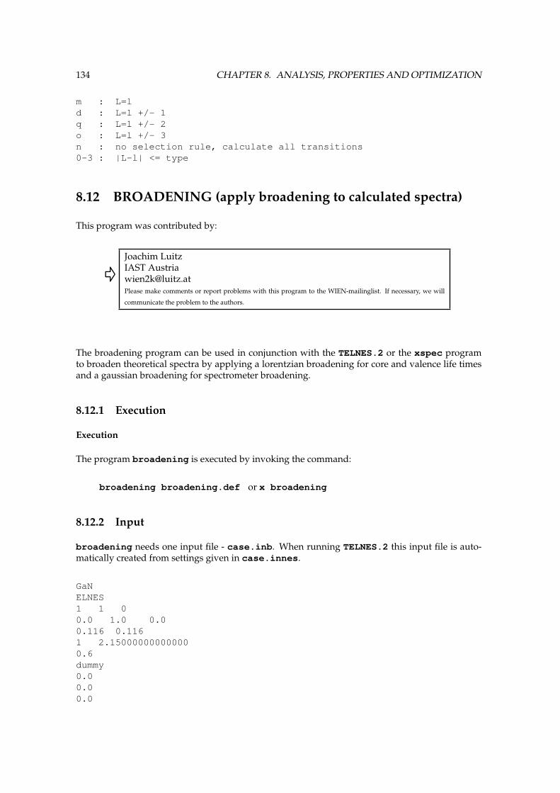
134 CHAPTER 8. ANALYSIS, PROPERTIES AND OPTIMIZATION
m : L=ld : L=l +/- 1q : L=l +/- 2o : L=l +/- 3n : no selection rule, calculate all transitions0-3 : |L-l| <= type
8.12 BROADENING (apply broadening to calculated spectra)
This program was contributed by:
Joachim LuitzIAST [email protected] make comments or report problems with this program to the WIEN-mailinglist. If necessary, we will
communicate the problem to the authors.
The broadening program can be used in conjunction with the TELNES.2 or the xspec programto broaden theoretical spectra by applying a lorentzian broadening for core and valence life timesand a gaussian broadening for spectrometer broadening.
8.12.1 Execution
Execution
The program broadening is executed by invoking the command:
broadening broadening.def or x broadening
8.12.2 Input
broadening needs one input file - case.inb. When running TELNES.2 this input file is auto-matically created from settings given in case.innes.
GaNELNES1 1 00.0 1.0 0.00.116 0.1161 2.150000000000000.6dummy0.00.00.0

8.13. OPTIMIZE 135
line value explanation1 ‘GaN ...’ Title (of no consequence for the calculation)2 ELNES — ABS — EMIS Type of input spectrum3 NC C1 C2 specification of input file: NC number of columns
to read, C1 and C2 column to broaden (only in“ELNES” mode)
4 SPLIT XINT1 XINT2 split energy, XINT1—2 relative intensities of spectrain C1 and C2
5 GA GB core hole lifetime of the two edges6 W WSHIFT W: type of valence broadening (1: linear with E/10,
2: Muller like E2), edge offset7 S Spectrometer broadening FWHM in eV8 dummy dummy keyword for compatibility with lorentz9-11 E0, E1, E2 quadratic energy dependent broadening (only used
for type ELNES and EMIS when selecting valencebroadening type W=2)
8.13 OPTIMIZE (Volume, c/a or 2-4 dimensional lattice parameteroptimization)
This program generates a series of new struct files corresponding to different volumes, c/a ratios,or otherwise different lattice parameters (depending on your input choice) from an existing structfile (either case initial.struct or case.struct). (When case initial.struct is notpresent, it will be generated from the original case.struct.
Furthermore it produces a shell script optimize.job. You may modify this script and execute it.Further analysis of the results (at present only equilibrium volume or c/a ratio are supported inw2web) allows to find the corresponding equillibrium parameters (see Sec.5.3.1).
8.13.1 Execution
The program optimize is executed by invoking the command:
optimize optimize.def or x optimize
8.13.2 Input
You have to specify interactively which task should be performed (volume, c/a, b/a optimization,or full optimization for tetragonal, orthorhombic or monoclinic structure), how many cases youwant to do and how large the change (+/- xx %) should be for each case.
8.14 ELAST (Elastic constants for cubic cases)
This program was contributed by:

136 CHAPTER 8. ANALYSIS, PROPERTIES AND OPTIMIZATION
Thomas CharpinLab. Geomateriaux de l’IPGP, Paris, France(In September 2001 we received the sad notice that Thomas Charpin died in acar accident).Please make comments or report problems with this program to the WIEN-mailinglist. If necessary, we will
communicate the problem to the authors.
This package calculates elastic constants for cubic crystals. It is described in detail by the author inCharpin 2001.
8.14.1 Execution
The package is driven by three scripts:
I init elast:It prepares the whole calculation and should be run in a directory with a valid case.structand case.inst file. It creates the necessary subdirectories elast, elast/eos,elast/tetra, elast/rhomb, elast/result, the templates for tetragonal and rhombo-hedral distortion and initializes the calculations using init lapw.
I elast setup:It should be run in the elast directory, generates the distorted struct-files and eos.job,rhomb.job and tetra.job. These scripts must be adapted to your needs (spin-polarization, convergence,...) and run. elast setup can be run several times (for differentdistortions,...).
I ana elast:Once all calculations are done, change into elastresult and run this script. The finalresults are stored in elastresultoutputs.
I genetempl, setelast, anaelast:These three small programs are called by the above scripts.
8.15 MINI (Geometry minimization)
This program is usually called from the script min lapw and performs movements of theatomic positions according to the calculated forces (please read Sec. 5.3.2). It generates a newcase.struct file which can be used in the next geometry/time step. Depending on the input op-tions, mini helps to find the equilibrium positions of the atoms or performs a molecular dynamicssimulation (which might take very long time).
For finding the equilibrium positions different methods are available. We recommendPORT, a “reverse-communication trust-region Quasi-Newton method” from the Port library(http://www.bell-labs.com/project/PORT/doc/port3doc.tar.gz, Gay 1983), which was imple-mented by L.D.Marks ([email protected], http://www.numis.northwestern.edu). Itminimizes the total energy and NOT the forces (using the forces as derivative of E vs. atomicpositions). In cases when energy and forces are not ”compatible”, eg. because of numerical noisedue to limited scf convergence, small RKmax or crude k-mesh, PORT may fail. An interesting al-ternative is a sophisticated modified steepest-descent method (NEW1), which minimizes the forces(does not use the total energy). Eventually a damped Newton dynamics is also available.
The forces are read from a file case.finM, while the “history” of the geometry optimization orMD is stored in case.tmpM

8.15. MINI 137
One can constrain individual positions in case.inM or define linear constrains for several posi-tions using case.constraint (thanks to B.Yanchitsky (Kiev, [email protected]); for details seecomments in the SRC templates/case.constraint file). In case of constraint calculations one shoulduse NEW1 (in case.inM) or, when PORT is used, do not use pairhess and remove files like.minrestart, .min hess, .minpair.
8.15.1 Execution
The program mini is executed by invoking the command:
mini mini.def or x mini
8.15.2 Dimensioning parameters
The following dimensioning parameters are collected in the file param.inc:
MAXIT maximum number of geometry stepsNRAD number of radial mesh pointsNCOM number of LM terms in densityNNN number of neighboring atoms for nnNSYM order of pointgroup
8.15.3 Input
Two examples are given below; one for a PORT geometry optimization, and one for moleculardynamics using a NOSE thermostat:
Input for geometry optimization:
---------------- top of file: xxx.inM --------------------PORT 2.0 0.25 (PORT/NEWT tolf step0 (a4,2f5.2))1.0 1.0 1.0 3.0 ( 1..3:delta, 4:BO/eta(1=friction zero))1.0 1.0 1.0 6.0 ( 1..3=0 constraint)------------------- bottom of file ------------------------
Interpretive comments on this file are as follows.
line 1: format(a4,2f5.2)
MINMOD Modus of the calculationPORT Geometry optimization with reverse-communication trust-region
Quasi-Newton routine from the Port library. Recommended option.NEW1 Performs geometry optimization with ”sophisticated” steepest-descent
method with automatic adaptation of stepsize (still experimental, butwhen PORT fails, an interesting alternative)
NEWT Performs geometry optimization with damped Newton scheme accord-ing toRτ+1
m = Rτm + ηm(Rτ
m −Rτ−1m ) + δmF
τm
whereRτm and F τ
m are the coordinate and force at time step τ . When theforce has changed its direction from the last to the present timestep (oris within the tolerance TOLF), ηm will be set to 1 − ηm. Please see alsothe comments in Sect. 5.3.2

138 CHAPTER 8. ANALYSIS, PROPERTIES AND OPTIMIZATION
BFGS Performs geometry optimization with the variable metric method ofBFGS. This option works only when a quadratic approximation is agood approximation to the specific potential surface. Obsolete.
TOLF Force tolerance, geometry optimization will stop when all forces arebelow TOLF.
STEP0 Initial ”Trust-region radius”. Determines size of first geometry step.
line 2: free format
DELTA(1-3)
For PORT (and BFGS): Precondition parameters, determine the size ofthe first geometry stepFor NEWT/NEW1: x,y,z-delta parameters. Determines speed of mo-tion. Good values must be found for each individual system. They de-pend on the atomic mass, the vibrational frequencies and the startingpoint (see Sect. 5.3.2).DELTA(i) = 0 constrains the corresponding i-th coordinate (use NEW1to ensure this constrain). The delta-x,y,z correspond to the global co-ordinates (the same as the positions in case.struct and the forces:FGL from case.scf).Whenever you change these DELTA(i) you must remove file case.tmpM !
ETA For PORT: Bond-order parameter: should be set approximately to thenumber of nearest neighbors (or left at 1.).For NEWT: damping (friction) parameter. ETA=1 means no friction,ETA=0 means no speed from previous time stepsFor NEW1: ETA is not used
>>> line 2: must be repeated for every atom
Input for Molecular dynamics:
---------------- top of file: nbc.inM --------------------NOSE (NOSE/MOLD (a4))58.9332 400. 1273. 5.0 (Masse, delta t, T, nose-frequency)58.9332 400. 1273. 5.058.9332 400. 1273. 5.058.9332 400. 1273. 5.058.9332 400. 1273. 5.058.9332 400. 1273. 5.0------------------- bottom of file ------------------------
Interpretive comments on this file are as follows.
line 1: format(a4,f5.2)
MINMOD Modus of the calculationMOLD Performs next molecular dynamics timestepNOSE Performs next molecular dynamics timestep using a NOSE thermostat
line 2: free format
MASS Atomic mass of ith atomTIMESTEP Time step of MD (in atomic units, depends on highest vibrational fre-
quencies)
TEMP Simulation Temperature (K)
8.16. OPTIC 139
NOSF Nose-frequency
>>>line 2: must be repeated for every atom
8.16 OPTIC (calculating optical properties)
This program was contributed by:
Claudia Ambrosch-DraxlAtomistic Modelling and Design of MaterialsUniversity LeobenA-8700 Leoben, AUSTRIAemail: [email protected] make comments or report problems with this program to the WIEN-mailinglist. If necessary, we will
communicate the problem to the authors.
The theoretical background is described in detail in Ref. Abt 1994 and Ambrosch-Draxl 06 (Pleasecite the latter when publishing optics results!). The calculation of optical properties requires adense mesh of eigenvalues and the corresponding eigenvectors. For that purpose start kgen andgenerate a fine k-mesh (with many k-points). Run lapw1 and then lapw2 with the option FERMI(Note: You must also put TETRA / with value=101. for metallic systems case.in2) in order to generatethe weight-file. After the vector-file has been generated by lapw1 run optic in order to producethe momentum matrix elements. Then the program joint carries out the BZ integration andcomputes the imaginary part of the complex dielectric tensor. In order to obtain the real part of thedielectric tensor kram may be executed which uses the Kramers-Kronig relations.
The program optic generates the symmetrized squared momentum matrix elements
Mi =< n′~k|~p.~ei| n~k >2
between all band combinations for each k-point given in the vector-file and stores them incase.symmat. For the orthogonal lattices the squared diagonal components can be found in thefile case.mat diag. For non-orthogonal systems all 6 components (Mj)∗Mk can be calculatedaccording to the symmetry of the crystal. In systems without inversion symmetry the complexversion opticc must be executed.
The matrix elements (and the imaginary part of the dielectric tensor) are given per spin in caseof the spin-polarized calculation and as a sum of both spin directions if the calculation is non-spinpolarized.
Due to spin-orbit coupling imaginary parts of the nondiagonal elements may occur in spinpolar-ized cases. Thus in general, up to 9 components can be calculated at the same time.
You must not use p-1/2 “relativistic” LOs in LAPWSO, since this basis is not supported on OPTICS yet.
8.16.1 Execution
The program optic is executed by invoking the command:
optic(c) optic.def or x optic [-c -up|dn -so -p]

140 CHAPTER 8. ANALYSIS, PROPERTIES AND OPTIMIZATION
Recommended procedure for spin-orbit coupling:
In order to get the correct matrix elements, the files case.vectorso[up|dn] have to be used.For that purpose the following procedure is recommended:
I run SCF cycle: run[sp] lapw -soI generate a fine k-mesh for the optics part: x kgen [-so (if case.ksym has been
created by symmetso) ]I change TOT to FERMI in case.in2cI execute run[sp] lapw -so -s lapw1 -e lcore with this fine k-meshI run optic: x opticc -so [-up]I run joint: x joint [-up]I run kram: x kram [-up]
In cases of non-spinpolarized calculations WITHOUT inversion symmetry AND spin-orbit cou-pling, one must do some tricks and “mimick” a spinpolarized calculation:
I cp case.vsp case.vspupI cp case.vsp case.vspdnI cp case.vectorso case.vectorsoupI x lapw2 -fermi -so -cI cp case.weight case.weightupI cp case.weight case.weightdnI x optic -so -upI x joint -up
Due to the “paramagnetic” weight files (which are normalized to 2 electrons per band instead ofone) all your results (joint/sigma...) must be divided by a factor of two.
Note: In spin-polarized cases with spin-orbit only one call to optic, joint and/or kram (either up ordown) is necessary, since the spins are not independent any more and both vector-files are used at the sametime.
8.16.2 Dimensioning parameters
The following dimensioning parameters (listed in param.inc r and param.inc c) are used:
LMAX highest l+1 in basis function inside sphere (consistent with input in case.in1)LOMAX highest l for local orbital basis (consistent with input in case.in1)NRAD number of radial mesh pointsNSYM order of point group
8.16.3 Input
An example is given below:
---------------- top of file: case.inop --------------------99999 1 : NKMAX, NKFIRST-5.0 2.0 : EMIN, EMAX2 : number of choices (columns in *symmat)1 : Re xx3 : Re zzOFF : ON/OFF writes MME to unit 4------------------- bottom of file -------------------------
8.16. OPTIC 141
Interpretive comments on this file are as follows:
line 1: free format
nkmax,nkfirst
maximal number of k-points , number of k-point to start calculation
line 2: free format
emin,emax
absolute energy range (Ry) for which matrix elements should be calcu-lated
line 3: free format
ncol number of choices (columns in case.symmat)
line 4+: free format
icol column to select. Choices are:1 . . . Re < x >< x >2 . . . Re < y >< y >3 . . . Re < z >< z >4 . . . Re < x >< y >5 . . . Re < x >< z >6 . . . Re < y >< z >7 . . . Im < x >< y >8 . . . Im < x >< z >9 . . . Im < y >< z >Options 7-9 apply only in presence of SO, options 4-6 only in non-orthogonal cases.
line 5: free format
IMME OFF/ON; optionally prints unsquared momentum matrix elements tounit 4

142 CHAPTER 8. ANALYSIS, PROPERTIES AND OPTIMIZATION
8.17 JOINT (Joint Density of States)
This program was contributed by:
Claudia Ambrosch-DraxlAtomistic Modelling and Design of MaterialsUniversity LeobenA-8700 Leoben, AUSTRIAemail: [email protected] make comments or report problems with this program to the WIEN-mailinglist. If necessary, we will
communicate the problem to the authors.
This program carries out the BZ integration using the momentum matrix elements calculated be-fore by optic. The interband or the intraband contributions to the imaginary part of the dielectrictensor (ε2) can be computed. Alternatively, the DOS or the joint DOS can be derived.
The output in case.joint can be plotted with an xy-plotting package.
Warning: Negative values for ε2 may occur due to negative weights in Blochl’s tetrahedron method.
8.17.1 Execution
The program joint is executed by invoking the command:
joint joint.def or x joint [-up|dn]
8.17.2 Dimensioning parameters
The following parameter is listend in files param.inc:
NSYM order of point groupMG0 number of columns (usually 9)
8.17.3 Input
An example is given below:
---------------- top of file: case.injoint -----------------------1 9999 8 : LOWER,UPPER,upper-valence BANDINDEX
-0.0000 0.00100 2.0000 : EMIN DE EMAX FOR ENERGYGRID IN rydeV : output units eV / ryd
4 : SWITCH2 : NUMBER OF COLUMNS
0.1 0.1 0.3 : BROADENING (FOR DRUDE MODEL - switch 6,7)------------------- bottom of file -------------------------------
Interpretive comments on this file are as follows:
line 1: free format
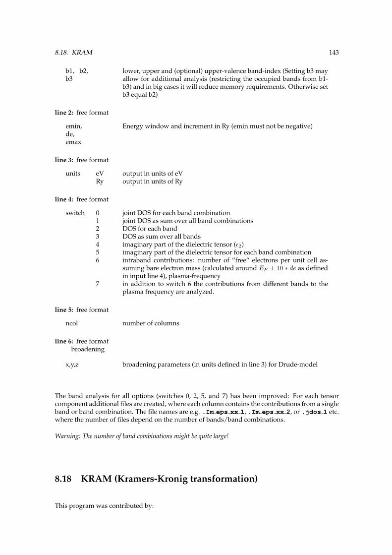
8.18. KRAM 143
b1, b2,b3
lower, upper and (optional) upper-valence band-index (Setting b3 mayallow for additional analysis (restricting the occupied bands from b1-b3) and in big cases it will reduce memory requirements. Otherwise setb3 equal b2)
line 2: free format
emin,de,emax
Energy window and increment in Ry (emin must not be negative)
line 3: free format
units eV output in units of eVRy output in units of Ry
line 4: free format
switch 0 joint DOS for each band combination1 joint DOS as sum over all band combinations2 DOS for each band3 DOS as sum over all bands4 imaginary part of the dielectric tensor (ε2)5 imaginary part of the dielectric tensor for each band combination6 intraband contributions: number of “free“ electrons per unit cell as-
suming bare electron mass (calculated around EF ± 10 ∗ de as definedin input line 4), plasma-frequency
7 in addition to switch 6 the contributions from different bands to theplasma frequency are analyzed.
line 5: free format
ncol number of columns
line 6: free formatbroadening
x,y,z broadening parameters (in units defined in line 3) for Drude-model
The band analysis for all options (switches 0, 2, 5, and 7) has been improved: For each tensorcomponent additional files are created, where each column contains the contributions from a singleband or band combination. The file names are e.g. .Im eps xx 1, .Im eps xx 2, or .jdos 1 etc.where the number of files depend on the number of bands/band combinations.
Warning: The number of band combinations might be quite large!
8.18 KRAM (Kramers-Kronig transformation)
This program was contributed by:

144 CHAPTER 8. ANALYSIS, PROPERTIES AND OPTIMIZATION
Claudia Ambrosch-DraxlAtomistic Modelling and Design of MaterialsUniversity LeobenA-8700 Leoben, AUSTRIAemail: [email protected] make comments or report problems with this program to the WIEN-mailinglist. If necessary, we will
communicate the problem to the authors.
The Kramers-Kronig analysis is carried out for the actual number of columns contained in thecase.joint[up|dn] file. For each real component its imaginary counterpart is created and viceversa. All dielectric tensor components can be found in file case.epsilon[up|dn]. The real andimaginary parts of the optical conductivity (in 1015/s) are written to file case.sigmak[up|dn].In addition, file case.absorp contains the real parts of the optical conductivity (in 1/(Ωcm) andthe absorption coefficients. The loss function is also calculated (case.eloss), where for the pre-viously calculated Plasma-frequency the intraband contributions can be added.
Please note, that for spin-polarized calculations, the Kramers-Kronig analysis is NOT really addi-tive, i.e. most quantities (like ε1) cannot be obtained by simply adding the spin-up and dn resultsto get the total contribution (see equations in Ambrosch 06). Thus, one should add up both spincontributions of ε2 (in case.jointup and case.jointdn) using addjoint-updn lapw (thiswill produce case.joint) before calling (non-spinpolarized) x kram.
The 3 sumrules are also checked and written to case.sumrules.
The output in case.epsilon[up|dn] and case.sigmak[up|dn] can be plotted with any xy-plotting package, opticplot lapw or the ”OPTIC”-task in w2web.
8.18.1 Execution
The program kram is executed by invoking the command:
kram kram.def or x kram [-up|dn]
8.18.2 Dimensioning parameters
The following parameters are listed in files param.inc:
MAXDE maximum number of points in energy meshMPOL fixed at 6
8.18.3 Input
An example is given below:
---------------- top of file: case.inkram -----------------------0.0 gamma for Lorentz broadening (in units selected in joint)0.0 energy shift (scissors operator) (in units selected in joint)1 add intraband contributions? yes/no: 1/0
12.60 plasma frequencies (for each ‘‘column’’ in case.injoint)0.20 Gammas for Drude terms (for each ‘‘column’’ in case.injoint)
------------------- bottom of file -------------------------------
Interpretive comments on this file are as follows:

8.19. FSGEN 145
line 1: free format
EGAMM Lorentz broadening (in energy units selected in joint)
line 2: free format
ESHIFT Energy shift (scissors operator) (in energy units selected in joint)
line 3: free format
INTRA 0 Intraband contributions are not added1 Intraband contributions are added (requires plasma-frequencies calcu-
lated by joint using switch “6”) )
line 4: free format
EPL Plasma-frequencies (calculated by joint using SWITCH=6 for allcolumns)
line 5: free format
EDRU Broadening for Drude terms (for all columns)
8.19 FSGEN (Fermi-surface generation)
Unfortunately there is no really versatile tool for Fermi surface generation or analyzing FS proper-ties. We have collected here a series of small programs together with some description on how toproceed to generate 2D-Fermisurfaces within WIEN.
I As usually, you have to run an scf cycle and determine a good Fermi-energy. ”Good” meanshere a Fermi-energy coming from a calculation with a dense k-mesh.
I You should than create a mesh within a plane of the BZ, where you want to plot the FS. Someutility programs like sc fs mesh, (fcc, bcc, cxz mon and hex are also available) may helpyou here, but only some planes of the BZ have been implemented so far. Please check thesesimple programs and modify them according to your needs. Insert the generated k-meshfort.2 into case.in1.
I Run lapw1 with this k-mesh.I Run spaghetti with input-options such that it prints the bands which intersect EF to
case.spaghetti ene (line 10, see sec. 8.3)I Edit case.spaghetti ene and insert a line at the top:
NX, NY, x-len, y-len, NXinter, NYinter, Invers, FlipwhereNX, NY are the number of points in the two directionsx-len, y-len are the length of the two directions of the plane (in bohr−1, you can find this incase.spaghetti ene)NXinter, NYinter: interpolated mesh, e.g. 2*NX-1Invers: 0/1: mirrors x,yFLIP: 0/1: flips x,y to y,x
I Run spagh2rho < case.spaghetti ene to convert from this format into a format whichis compatible with the case.rho file used for charge density plotting. It generates filesfort.11, fort.12, ... (for each band separately) and you should use your favorite plotting

146 CHAPTER 8. ANALYSIS, PROPERTIES AND OPTIMIZATION
program to generate a contourplot of the FS (by using a contourlevel = 0). Alternatively youcan use for plotting:
I Run fsgen lapw 11 xx save filename, which is a small shell script that can plot allfermi surfaces using the data-files fort.11, fort.12, ... fort.xx generated in the pre-vious steps. It requires the public domain package pgplot and the contour-plot programplotgenc. (The latter can be obtained from P. Blaha ([email protected]), butyou must have installed pgplot before.)

9 Utility Programs
Contents9.1 symmetso . . . . . . . . . . . . . . . . . . . . . . . . . . . . . . . . . . . . . . . . . 1479.2 pairhess . . . . . . . . . . . . . . . . . . . . . . . . . . . . . . . . . . . . . . . . . . . 1489.3 afminput . . . . . . . . . . . . . . . . . . . . . . . . . . . . . . . . . . . . . . . . . . 1499.4 clmcopy . . . . . . . . . . . . . . . . . . . . . . . . . . . . . . . . . . . . . . . . . . . 1509.5 reformat . . . . . . . . . . . . . . . . . . . . . . . . . . . . . . . . . . . . . . . . . . 1529.6 hex2rhomb and rhomb in5 . . . . . . . . . . . . . . . . . . . . . . . . . . . . . . . 1529.7 plane . . . . . . . . . . . . . . . . . . . . . . . . . . . . . . . . . . . . . . . . . . . . 1529.8 add columns . . . . . . . . . . . . . . . . . . . . . . . . . . . . . . . . . . . . . . . . 1529.9 clminter . . . . . . . . . . . . . . . . . . . . . . . . . . . . . . . . . . . . . . . . . . . 1529.10 eosfit . . . . . . . . . . . . . . . . . . . . . . . . . . . . . . . . . . . . . . . . . . . . 1539.11 eosfit6 . . . . . . . . . . . . . . . . . . . . . . . . . . . . . . . . . . . . . . . . . . . . 1539.12 spacegroup . . . . . . . . . . . . . . . . . . . . . . . . . . . . . . . . . . . . . . . . . 1539.13 xyz2struct . . . . . . . . . . . . . . . . . . . . . . . . . . . . . . . . . . . . . . . . . 1549.14 cif2struct . . . . . . . . . . . . . . . . . . . . . . . . . . . . . . . . . . . . . . . . . . 1549.15 struct2cif . . . . . . . . . . . . . . . . . . . . . . . . . . . . . . . . . . . . . . . . . . 1549.16 StructGen of w2web . . . . . . . . . . . . . . . . . . . . . . . . . . . . . . . . . . . 1559.17 supercell . . . . . . . . . . . . . . . . . . . . . . . . . . . . . . . . . . . . . . . . . . 1559.18 structeditor . . . . . . . . . . . . . . . . . . . . . . . . . . . . . . . . . . . . . . . . . 1559.19 Visualization . . . . . . . . . . . . . . . . . . . . . . . . . . . . . . . . . . . . . . . . 157
9.1 symmetso
This program helps to setup spin-orbit calculations in magnetic systems. Since SO may break sym-metry in certain spacegroups, it classifies your symmetry operations into operations A, which donot invert the magnetization (identity, inversion, rotations with the rotation axis parallel to magne-tization), B, which invert it (mirror planes) and C, which change the magnetization in some otherway. (Note: magnetization is a result of a circular current, or equivalently, an axial vector result-ing from a vector product z ∼ x × y). symmetso will keep all A-type and throw away all C-typesymmetry operations. Depending on the presence of inversion symmetry it will keep (inversionis present) or remove the B-type operations. Finally, symmetso uses the remaining symmetry op-erations to check/generate equivalent atomic positions (it can happen that some equivalent atomsbecome non-equivalent after inclusion of SO interaction).
In essence, it reads your case.struct and case.inso (for the direction of magnetization) filesand creates an ordered case.struct orb file with proper symmetry and equivalent atoms. It alsogenerates a file case.ksym, which is a struct file with valid operations to generate a proper k-mesh
147

148 CHAPTER 9. UTILITY PROGRAMS
using ’’x kgen -so’’. In addition proper input files case.in1, case.in2, case.inc,case.vspup/dn, case.vnsup/dn, case.clmsum, case.clmup/dn are generated, so thatyou can continue with runsp -so without any further changes.
9.1.1 Execution
The program symmetso is executed by invoking the command:
symmetso symmetso.def or x symmetso [-c]
Usually it is called from the script initso lapw and thus needs not to be invoked manually.
9.2 pairhess
This program was contributed by:
James Rondinelli, Bin Deng and Laurence MarksDept. Materials Science and EngineeringNorthwestern UniversityEvanston, [email protected] make comments or report problems with this program to the WIEN-mailinglist. If necessary, we will
communicate the problem to the authors.
This program creates an approximate hessian matrix (in .minpair) for structure minimizationusing the PORT option. It uses a harmonic model with exponentially decaying bond strenght andin many cases reduces the number of geometry steps during min lapw significantly. It is describedin detail in Rondinelli et al. 2006.
For its usage see the comments in sect. 5.3.2.
Please note, R (rhombohedral) lattices are not supported yet.
9.2.1 Execution
The program pairhess is executed by invoking the command:
pairhess pairhess.def or x pairhess
9.2.2 Dimensioning parameters
The following parameters are used in param.inc:
NATMAX max. number of atoms)NEIGMAX max number of neighbours

9.3. AFMINPUT 149
9.2.3 Input
pairhess uses an optional input file case.inpair, which is needed only for an experienceduser for better tailoring of certain default parameters (when the ”condition number” is larger than3, or ”max. eigenvalue” .gt. 3).
An example is given below:
---------------- top of file: case.inpair -----------------------10.0 2.0 0.25 (Rmax, Decay, ReScale)0.05 1.0 0 (Cutoff, Diag, mode)
Interpretive comments on this file are as follows:
line 1: free format
RMAX Maximum distance (a.u.) for considering neighbors. 8-12 is good.
DECAY Exponential decay applied to neighbors when calculating the pairwisebond strenghts. 1.5-2.5 is reasonable.
RESCALE A scaling term to multiply the pairwise hessian by. This number israther important; 0.25 appears to be best, 0.35 is more conservative
line 2: free format
CUTOFF When the weighting (via an exponential decay) becomes smaller thanthis number the pairwise bonds are ignored.
DIAG The value to multiply a unitary matrix by, this is added to the hessianestimate
MODE 0: Harmonic model; [1: spring model; not working]
9.3 afminput
This program creates the inputfile case.inclmcopy st for the program clmcopy, which copiesspin-up densities of atom i to spin-down densities of the related antiferromagnetic atom j and viceversa in an anti-ferromagnetic system. It uses a symmetry operation to find out how and whichatomic densities must be interchanged and how the Fourier coefficients of the density transform.It is based on the ideas of Manuel Perez-Mato (Bilbao, Spain).
See $WIENROOT/SRC afminput/afminput test for several examples.
The best way is to supply a file case.struct supergroup, which is the struct file of the non-magnetic supergroup. If the two spacegroups are “TRANSLATIONENGLEICH”, it will find outautomatically the proper symmetry operation. Please note, this automatic way works only when thecoordinate system remains identical. In some cases sgroup may interchange eg. the y and z axis. In suchcases reverse this change, both, for the lattice parameters as well as for all positions, set NSYM=0 and runinit lapw again (ignoring any suggestion of sgroup).

150 CHAPTER 9. UTILITY PROGRAMS
If the two spacegroups are “KLASSENGLEICH” (i.e. have the same number of symmetry opera-tions), you will be asked to supply a translation which transforms the AF atoms into each other.A typical example would be bcc Cr: the bcc supergroup and the AF subgroup (simple cubic) haveboth 48 symmetry operations and the proper translation is (0.5,0.5,0.5).
Finally, if you don’t give case.struct supergroup, you have to supply a symmetry operation(rotation + non-primitive translation) as input. For bcc Cr or the famous NiO-AFII structure thiswould be simply 1.0 0.0 0.0
0.0 1.0 0.00.0 0.0 1.0
0.50.50.5
Please see the comments in sect. 4.5.4 on how to proceed in detail for AFM calculations and findfurther examples in SRC afminput.
9.3.1 Execution
The program afminput is executed by invoking the command:
afminput afminput.def or x afminput
9.3.2 Dimensioning parameters
The following parameters are used:
NCOM number of LM components in the density (in param.inc)LMAX max l for LM expansion of the density (in param.inc).
9.4 clmcopy
This program generates the spin-dn density (case.clmdn) from a given spin-up density(case.clmup) according to rules and symmetry operations in case.inclmcopy (generated ear-lier by afminput) for an AFM calculation.
Please see the comments in sect. 4.5.4 on how to proceed in detail for AFM calculations.
9.4.1 Execution
The program clmcopy is executed by invoking the command:
clmcopy clmcopy.def or x clmcopy
9.4.2 Dimensioning parameters
The following parameters are used in param.inc:
NCOM number of LM components in the densityNRAD number of radial mesh pointsNSYM number of symmetryoperations

9.4. CLMCOPY 151
9.4.3 Input
An example is given below:
---------------- top of file: case.inclmcopy -----------------------2 NUMBER of ATOMS to CHANGE1 2 INTERCHANGE these ATOMS
-1.00000000000 0.00000000000 0.00000000000 SYMMETRY OPERATION0.00000000000 -1.00000000000 0.000000000000.00000000000 0.00000000000 -1.000000000000 NUMBER of LM to CHANGE SIGN3 4 INTERCHANGE these ATOMS
-1.00000000000 0.00000000000 0.00000000000 SYMMETRY OPERATION0.00000000000 -1.00000000000 0.000000000000.00000000000 0.00000000000 -1.000000000009 NUMBER of LM to CHANGE SIGN
1 0 1 0 -1.003 0 3 0 -1.003 2 3 2 -1.00
-3 2 -3 2 -1.005 0 5 0 -1.005 2 5 2 -1.00
-5 2 -5 2 -1.005 4 5 4 -1.00
-5 4 -5 4 -1.001 0 0 0.500000 1 0 0.000000 0 1 0.50000
Interpretive comments on this file are as follows:
line 1: free format
NATOM Number of atoms for which rules for copying the density will be de-fined
line 2: free format
N1, N2 Interchange spin-up and dn densities of atoms N1 and N2
line 3-5: free format
SYM Symmetry operation for atom N1 to rotate into N2 (without transla-tional part)
line 6: free format
NLM Number of LM values, for which you have to change the sign whenswapping up and dn-densities
line 7ff: free format
L1,M1,L2,M2,Fac NLM pairs of L1,M1 (spin-up), which change into L2,M2 (spin-dn) andthe respecting CLMs are multiplied by Fac
Lines 2-7ff have to be repeated NATOM times.line 8-10: free format
SYM0 Symmetry operation (one of the operations of the NM-supergroupmissing in the AFM-subgroup (transfers spin-up into spin-dn atom)

152 CHAPTER 9. UTILITY PROGRAMS
9.5 reformat
To produce a surface plot of the electron density using rhoplot lapw (which is an interface tognuplot), data from the file case.rho created by lapw5 must be converted using reformat
The sources of the program reformat.c are supplied in SRC reformat.
9.6 hex2rhomb and rhomb in5
hex2rhomb interactively converts the positions of an atom from hexagonal to rhombohedral coor-dinates (needed in case.struct).
rhomb in5 interactively helps to generate input case.in5 for density plots with lapw5 for rhom-bohedral systems. It defines a plane as needed in the input file when you specify 3 atoms of thatplane.
The sources of these programs are supplied in SRC trig.
9.7 plane
plane helps to generate case.in5 for density plots with lapw5 (for orthogonal and hex latticesonly). The plane will be specified by 3 atoms and you need an auxiliary file plane.input, whichcontains:
a,b,c # lattice parametersx0,y0,z0 # position of atom (fractional coordinates), which will be centered in the plotx1,y1,z1 # position of atom, which will be ‘‘below’’ the centered atomx2,y2,z2 # position of atom, which will show to the ‘‘left’’xl,yl # lenght (in bohr) of plot in x and y direction.’P’ # defines lattice, either P (carthesian coordinates) or H (hexagonal) supported
The source of this program is supplied in SRC trig.
9.8 add columns
add columns reads a sequence of pairs of 2 numbers (form stdin), adds them together and printsthe sum to stdout. If you have two columns of numbers in 2 files (eg. in colup and coldn) you canadd them using:
paste colup coldn | add columns > col
The source of this program is supplied in SRC trig.
9.9 clminter
clminter interpolates the density in case.clmsum/up/dn to a new radial mesh as defined incase.struct new. This utility is usefull when you run a structural minimization (min lapw),some atoms start to overlap and you have to reduce RMT (the size of the atomic spheres) of certainatoms. In such a case:

9.10. EOSFIT 153
I save the calculationsI generate case.struct new with modified RMTsI x clminterI in spinpolarized case repeat this line with -up and -dn switchesI cp case.struct new case.structI cp case.clmsum new case.clmsumI eventually copy also case.clmup/dn files)I run lapw; (it will probably take some iterations until you reach scf again, but it should be
much faster than starting with init lapw)
Note: Please be aware the the total energy will change with modified RMT (by some constant)and you must not compare energies comming from different RMTs (but most likely you can deter-mine the constant shift by repeating (at least) ONE calculation with identical structure but differentRMTs).
The source of this program is supplied in SRC trig.
9.10 eosfit
Small program to calculate the Equation of States (EOS; Equilibrium volume V0, Bulk modulus B0
and it’s derivative B′0. The Murnaghan (1944), the Birch-Murnaghan and the EOS2 equation of
states are supported. It relies on the file case.vol (containing lines with ”volume, E-tot”, usuallycreated from w2web using ”Volume optimization”), or alternatively is called from eplot lapwusing case.analysis (see 5.7.1 and 5.3.1).
The sources are supplied in SRC eosfit.
9.11 eosfit6
Nonlinear least squares fit (using PORT routines) for a parabolic fit of the energy vs. 2-4dim. lattice parameters. It requires case.ene and case.latparam, usually generated byparabolfit lapw. It can optionally produce case.enefit, which contains energies on a speci-fied grid for plotting purposes (in 2D same format as case.rho, which can be used in contourplotprograms). (See 5.3.1).
The sources are supplied in SRC eosfit6.
9.12 spacegroup
This program was contributed by:
Vaclav PetricekInstitute of PhysicsAcademy of Sciences of the Czech RepublicNa Slovance 2182 21 Praha (Prague) 8Czech [email protected] make comments or report problems with this program to the WIEN-mailinglist. If necessary, we will
communicate the problem to the authors.

154 CHAPTER 9. UTILITY PROGRAMS
Interactive program to generate equivalent positions for a given spacegroup and lattice. The pro-gram is also used internally from w2web to generate positions when selecting spacegroups in theStructGen.
9.13 xyz2struct
xyz2struct reads “atomlabel,x,y,z”-data from case.xyz and writes them intoxyz2struct.struct. You may have to edit the xyz-file and insert a switch ANG(default)/BOHRand a,b,c lattice parameters. Since xyz data contain no symmetry information, all atoms with thesame “label” will be treated as equivalent. The nuclear charges ZZ will not be given and you haveto insert them manually or use w2web-StructGen.
It is executed using:
xyz2struct < case.xyz
(I recommend this program only for cases with many non-equivalent atoms and (almost) no sym-metry. If you have spacegroup-information it is probably easier to use StructGen and copy/pasteof the positions).
A proper case.xyz file looks like:
ang7.47700 7.47700 7.47700B 4.98466667 1.24616667 0.00000000C 6.23083333 2.49233333 0.00000000.....
9.14 cif2struct
cif2struct reads structural data in cif-format from case.cif and writes them intocase.struct. It is executed using:
cif2struct case.cif
The required cif files can be for example be obtained from Cystallographic databases (e.g. theInorganic Crystal Structure DataBase ICSD) or from other programs.
Alternatively, cif2struct can work with case.txt, which contains the following data:
a # a..Ang, b..Bohr0.0 0.0 0.0 # shift of origin4.7554 4.7554 12.991 90. 90. 120. # a,b,c,angles
’R-3c’ # spacegroup-symbol (see \STRUCTGEN)’Al’ # atom-name0.0000000 0.0000000 0.3520000 # atomic position
’O’ # ...0.3063000 0.0000000 0.2500000 # ...
...
9.15 struct2cif
struct2cif creates a cif-file struct.cif from case.struct. It is executed using:
struct2cif
and will ask for the name of a struct file and a spacegroup. It was contributed by F. Boucher([email protected]).

9.16. STRUCTGEN OF W2WEB 155
9.16 StructGen of w2web
The new StructGen helps to generate the master input file case.struct. It has the followingadditional features:
I automatic conversion from/to A and BohrI Use spacegroup information (in conjunction with the spacegroup program (see 9.12 to gen-
erate equivalent positions)I built in calculator to carry out simple arithmetic operations to specify the position parameters
(of the equivalent atoms). Each position of equivalent atoms can be entered as a number, afraction (e.g. 1/3) or a simple expression (e.g. 0.21 + 1/3). The first position defines thevariables x, y and z, which can be using in expression defining the other positions (e.g. −y,x, −z + 1/2).
9.17 supercell
This program helps to generate supercells from a regular WIEN2k-struct file.
It asks interactively for the name of the original struct file and the number of cells in x, y, andz direction. (Only integers are allowed, thus no rotations by 45o like sqrt(2) x sqrt(2) cells aresupported yet).
If symmetry permits, one can change the target lattice to P, B or F centered lattices, (C and R typesnot yet supported), which allows to increase the number of atoms in these supercells by a factor of2, 4, 8, ...
If the target lattice is P, one can add some vacuum in each direction for slabs (or chains or isolatedmolecules) and also add a “top”-layer.
You can define an optional shift in x,y,z direction for all the atoms in the cell. (This might be usefullif you want to arrange the atoms in a certain way, eg. you may want to create a surface slab suchthat it is centered around z=0.5 (and not z=0), so that plotting programs (xcrysden) produce nicerpictures of the structure.
For the experienced user a much more flexible (but also more complicated) tool is available, namelythe structeditor package (see Sect.9.18).
Please note: You cannot make calculations with these supercells (except for surfaces) unless you modify thecreated supercell-struct file. You must break the symmetry by introducing some distortions (e.g. for a frozenphonon) or replace one atom by an impurity/vacancy, ....
9.17.1 Execution
The program supercell is executed by invoking the command:
supercell or x supercell
9.18 structeditor
This program was contributed by:
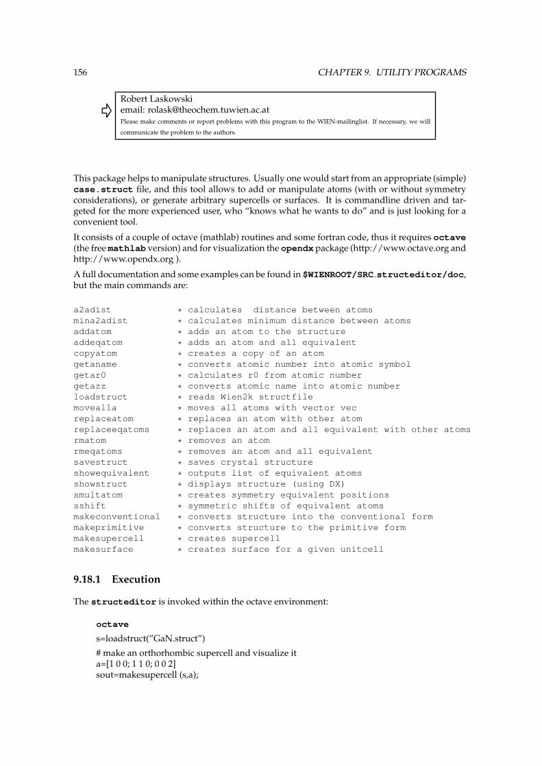
156 CHAPTER 9. UTILITY PROGRAMS
Robert Laskowskiemail: [email protected] make comments or report problems with this program to the WIEN-mailinglist. If necessary, we will
communicate the problem to the authors.
This package helps to manipulate structures. Usually one would start from an appropriate (simple)case.struct file, and this tool allows to add or manipulate atoms (with or without symmetryconsiderations), or generate arbitrary supercells or surfaces. It is commandline driven and tar-geted for the more experienced user, who “knows what he wants to do” and is just looking for aconvenient tool.
It consists of a couple of octave (mathlab) routines and some fortran code, thus it requires octave(the free mathlab version) and for visualization the opendx package (http://www.octave.org andhttp://www.opendx.org ).
A full documentation and some examples can be found in $WIENROOT/SRC structeditor/doc,but the main commands are:
a2adist * calculates distance between atomsmina2adist * calculates minimum distance between atomsaddatom * adds an atom to the structureaddeqatom * adds an atom and all equivalentcopyatom * creates a copy of an atomgetaname * converts atomic number into atomic symbolgetar0 * calculates r0 from atomic numbergetazz * converts atomic name into atomic numberloadstruct * reads Wien2k structfilemovealla * moves all atoms with vector vecreplaceatom * replaces an atom with other atomreplaceeqatoms * replaces an atom and all equivalent with other atomsrmatom * removes an atomrmeqatoms * removes an atom and all equivalentsavestruct * saves crystal structureshowequivalent * outputs list of equivalent atomsshowstruct * displays structure (using DX)smultatom * creates symmetry equivalent positionssshift * symmetric shifts of equivalent atomsmakeconventional * converts structure into the conventional formmakeprimitive * converts structure to the primitive formmakesupercell * creates supercellmakesurface * creates surface for a given unitcell
9.18.1 Execution
The structeditor is invoked within the octave environment:
octave
s=loadstruct(”GaN.struct”)
# make an orthorhombic supercell and visualize ita=[1 0 0; 1 1 0; 0 0 2]sout=makesupercell (s,a);
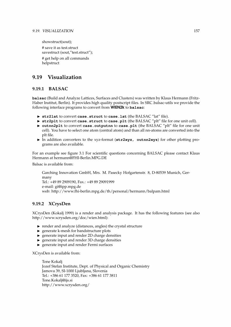
9.19. VISUALIZATION 157
showstruct(sout);
# save it as test.structsavestruct (sout,”test.struct”);
# get help on all commandshelpstruct
9.19 Visualization
9.19.1 BALSAC
balsac (Build and Analyze Lattices, Surfaces and Clusters) was written by Klaus Hermann (Fritz-Haber Institut, Berlin). It provides high quality postscript files. In SRC balsac-utils we provide thefollowing interface programs to convert from WIEN2k to balsac:
I str2lat to convert case.struct to case.lat (the BALSAC ”lat” file).I str2plt to convert case.struct to case.plt (the BALSAC ”plt” file for one unit cell).I outnn2plt to convert case.outputnn to case.plt (the BALSAC ”plt” file for one unit
cell). You have to select one atom (central atom) and than all nn-atoms are converted into theplt file.
I In addition converters to the xyz-format (str2xyz, outnn2xyz) for other plotting pro-grams are also available.
For an example see figure 3.1 For scientific questions concerning BALSAC please contact KlausHermann at [email protected]
Balsac is available from:
Garching Innovation GmbH, Mrs. M. Pasecky Hofgartenstr. 8, D-80539 Munich, Ger-manyTel.: +49 89 2909190, Fax.: +49 89 29091999e-mail: [email protected]: http://www.fhi-berlin.mpg.de/th/personal/hermann/balpam.html
9.19.2 XCrysDen
XCrysDen (Kokalj 1999) is a render and analysis package. It has the following features (see alsohttp://www.xcrysden.org/doc/wien.html):
I render and analyze (distances, angles) the crystal structureI generate k-mesh for bandstructure plotsI generate input and render 2D charge densitiesI generate input and render 3D charge densitiesI generate input and render Fermi surfaces
XCrysDen is available from:
Tone KokaljJozef Stefan Institute, Dept. of Physical and Organic ChemistryJamova 39, SI-1000 Ljubljana, SloveniaTel.: +386 61 177 3520, Fax: +386 61 177 [email protected]://www.xcrysden.org/

158 CHAPTER 9. UTILITY PROGRAMS
Figure 9.1: 3D electron density in TiC generated with XCrysDen

10 How to run WIEN2k for selectedsamples
Three test cases are provided in the WIEN2k package. They contain the two starting filescase.struct and case.inst and all the output so that you can compare your results withthem.
The test cases are the following (where the names correspond to what was called CASE in the restof this User’s Guide)
TiCFccniTiO2
We recommend to run these test cases (in a different directory) and compare the output to theprovided one. All test cases are setup such that the CPU-time remains small (seconds). For realproduction runs the value of RKMAX in case.in1must be increased and a better (denser) k-meshshould be used.
In addition we provide a subdirectory example struct files were various more complicatedstruct files can be found.
10.1 TiC
The TiC example is described in detail in chapter 3 (Quickstart).
10.2 Fcc Nickel (spin polarized)
Ferromagnetic Nickel is a test case for a spin-polarized calculation. Ni has the atomic configuration1s2, 2s2, 2p6, 3s2, 3p6, 3d8, 4s2 or [Ar] 3d8, 4s2. We treat the 1s, 2s, 2p and 3s as core states, and 3p(as local orbital), 3d, 4s and 4p are handled as valence states. In a spin-polarized calculation the filestructure and the sequence of programs is different from the non-spin-polarized case (see 4.5.2).
Create a new session and its corresponding directory. Generate the structure with the followingdata (we can use a large sphere as you will see from the output of nn):
159

160 CHAPTER 10. EXAMPLES
Title fcc NiLattice Fa 6.7 bohrb 6.7 bohrc 6.7 bohrα, β, γ 90Atom Ni, enter position (0,0,0) and RMT = 2.3
Initialize the calculation using the default RKmax and use 3000 k-points (a ferromagnetic metalneeds many k-points to yield reasonably converged magnetic moments). Allow for spin-polarization.
Start the scf cycle (runsp lapw) with ”-cc 0.0001” (in particular for magnetic systems charge con-vergence is often the best choice). At the bottom of the converged scf-file (Fccni.scf) you findthe magnetic moments in the interstital region, inside the sphere and the total moment per cell(only the latter is an “observable”, the others depend on the sphere size).
:MMINT: MAGNETIC MOMENT IN INTERSTITIAL = -0.03130:MMI001: MAGNETIC MOMENT IN SPHERE 1 = 0.66198:MMTOT: TOTAL MAGNETIC MOMENT IN CELL = 0.63068
10.3 Rutile (TiO2)
This example shows you how to “optimize internal parameters” and do a k-point parallel calcula-tion.
Create a new session and its corresponding directory. Generate the structure with the followingdata (we use a smaller O sphere because Ti-d states are harder to converge then O-p):
Title TiO2Spacegroup P42/mnm (136)a 8.682 bohrb 8.682 bohrc 5.592 bohrα, β, γ 90Atom Ti, enter position (0,0,0) and RMT = 2.0Atom O, enter position (0.3,0.3,0) and RMT = 1.6
StructGenshould automatically add the equivalent positions.
Initialize the calculation using RKmax=6.5 in tio2.in1 st and use 100 k-points and a “shift“ inkgen.
If you have more cpus available (a parallel machine or simply a couple of PCs with a common NFSfilesystem, for details see 5.5), you can use “Execution o Run scf”, activate the “parallel” button”and “start scf” in w2web. This will create and open a .machines file and you should insert lineswith the proper names of your PCs (possibly use 9 (or 3) processors since we have 9 k-points, ).Save this file and click on “Execution o Run scf”, activate “-fc 1.0” for force-convergence and “startscf” to submit the scf-cycle.
Alternatively at the command-line you can use the UNIX command
cp $WIENROOT/SRC_templates/.machines .
and edit this file. You would start the scf-cycle (in background) simply by typing
run_lapw -p -fc 1.0 &

10.4. SUPERCELL CALC 161
During the scf-cycle monitor tio2.dayfile and check convergence (:ENE, :DIS, :FGL002), eitherusing “Utils/Analysis” in w2web, or ‘‘grep :ENE tio2.scf’’. You should see some conver-gence of :FGL002 and then a big jump in the final cycle, when the valence-force corrections areadded. Only the last force (including this correction) is valid.
Since this force is quite large, you can now optimize the position of the O-atom:
Start the structure minimization in w2web using “Execution o mini.positions”. This will generateTiO2.inM, and you can try option PORT with tolf=1.0 (instead of 2.0), otherwise stay with thedefault parameters. Repeat “Execution o mini.positions” and start the minimization.
Alternatively you can use
min_lapw -p
which is identical to:
min_lapw -j ‘‘run_lapw -I -fc 1 -p’’
This will create TiO2.inM automatically, call the program min, which generates a new struct fileusing the calculated forces, and continues with the next scf cycle. It will continue until the forcesare below 1 mRy/bohr (TiO2.inM) and the final results are not “saved” automatically but can befound in the “current” calculation.
You should watch the minimization (:ENE, :FGL002, :POS002) using the file TiO2.scf mini,which contains the final iteration of each geometry step (see also Sec.5.3.2). If the forces in thisfile oscillate from plus to minus and seem to diverge, or if they change very little, you can editTiO2.inM (change the method, reduce or increase the stepsize), and remove TiO2.tmpM (con-tains the “history” of the minimization and is used to calculate the velocities of the moving atoms).(This should not be neceaasry for the rutile example, but may occur in more complex minimiza-tions. See comments in Sec. 5.3.2).
The final structural parameter of the O-atom should be close to x=0.304, which compares well withthe experimental x=0.305.
10.4 Supercell calculations on TiC
This example shows you how to create a supercell of TiC, which could be used to simulate a TiC-surface or vacancies, impurities or core-holes for X-ray absorption / ELNES spectroscopy. I’ll de-scribe the procedure using Unix and WIEN2k commands in an xterm, but of course you can do thesame in w2web.
Create a new directory, copy the original TiC struct file into it and run supercell program:
mkdir supercd supercp ../TiC/TiC.struct .x supercell
Specify “TiC.struct”, a “2x2x2” supercell, “F” lattice (this will create a cell with 16 atoms, you canalso create 32 or 64 atom cells using B or P lattice type. Note: surfaces require a P supercell).
cp TiC_super.struct super.struct
and edit this file to make some changes. You could eg.

162 CHAPTER 10. EXAMPLES
I delete an atom (to simulate a vacancy)I replace an atom by another element (impurity)I “label” an atom (put a 1 in the 3rd column next to the element name) to make this atom
unique (needed eg. for core-holes)I displace an atom (for phase transitions or phonons)
Note: it is important to make at least one of these chages. Otherwise the initialization will restore the originalunit cell (or the calculations will fail later on because symmetry is most likely not correct)
Run init lapw. You will see that nn complains and finds a new set of equivalent atoms (originallyall atoms were non-equivalent, but nn finds that some atoms have identical neighbors, thus shouldbe in an equivalent set). Accept the automatically generated struct file and continue. Remember,supercells normally require less k-points than the original small cell.
After the complete initialization you may in principle restore the original struct file (eg. without adisplacement) in case you want to “repeat” the undistorted structure in supercell geometry.
For a “core-hole” calculation you would now edit super.inc and remove one core electron fromthe desired atom and state (1s or 2p, ...). In addition you should add the missing electron eitherin super.inm (background charge) or super.in2 (add it to the valence electrons). In the lattercase, you should remove this extra electron AFTER scf and BEFORE calculation of the spectra.
Once this has been done, you could start a scf-cycle (for impurities, vacancies,.. you should mostlikely also optimize the internal positions).

Part III
Installation of the WIEN2k packageand Dimensioning of programs
163


11 Installation and Dimensioning
Contents11.1 Requirements . . . . . . . . . . . . . . . . . . . . . . . . . . . . . . . . . . . . . . . 16511.2 Installation of WIEN2k . . . . . . . . . . . . . . . . . . . . . . . . . . . . . . . . . . 16611.3 w2web . . . . . . . . . . . . . . . . . . . . . . . . . . . . . . . . . . . . . . . . . . . 16911.4 Environment Variables . . . . . . . . . . . . . . . . . . . . . . . . . . . . . . . . . . 171
11.1 Requirements
WIEN2k is written in FORTRAN 90 and requires a UNIX operating system since the programsare linked together via C-shell scripts. It has been implemented successfully on the followingcomputer systems: Intel Pentium PCs running under Linux, IBM RS6000, HP, SGI, DEC Alpha andSUN. Hardware requirements will change from case to case (small cases with 10 atoms per unit cellcan be run on a Pentium-II PC with 128 MB under Linux), but we recommend a more powerful PCor workstation with at least 256 MB (better 512 MM or more) memory and plenty of disk space (afew Gb).
For coarse grain parallization on the k-point level, a cluster of PCs with a 100 Mb/s network is suf-ficient. Faster communication is recommended for the fine grain (single k-point) parallel version.
In order to use all options and features (such as the new graphical user interface w2web or someof its plotting tools) the following public domain program packages in addition to a F90 compilermust be installed:
I perl 5 or higher (for w2web only)I emacs or another editor of your choiceI ghostscript (with jpg support)I gnuplot (with png support)I www-browserI pdf-reader, acroreadI MPI+SCALAPACK (for fine grain parallelization only)I Tcl/Tk-Toolkit (for Xcrysden only)
Usually these packages should be available on modern systems. If one of these packages is notavailable it can either be installed from public domain sources (ask your computing center, use theWWW to search for the nearest location of these packages) or the corresponding configuration maybe changed (e.g. using vi instead of emacs). None of the principal components of WIEN2k requiresthese packages, only w2web needs them.
165

166 CHAPTER 11. INSTALLATION AND DIMENSIONING
11.2 Installation of WIEN2k
11.2.1 Expanding the WIEN2k distribution
The WIEN2k package comes as a single tar file (or you can download about 50 individual tarfiles separately), which should be placed in a subdirectory which will be your $WIENROOT di-rectory (e.g. ./WIEN2k). In addition you can download three examples, namely TiC.tar.gz,TiO2.tar.gz and Fccni.tar.gz.
Uncompress and expand all files using:
tar -xvf wien2k 00.tar (skip this if you downloaded files separately)gunzip *.gzchmod +x ./expand lapw./expand lapw
You should have gotten the following directories:
./SRCSRC_afminputSRC_aimSRC_balsac-utilsSRC_broadeningSRC_cif2structSRC_clmaddsubSRC_clmcopySRC_dstartSRC_elastSRC_eosfitSRC_eosfit6SRC_filtvecSRC_fsgenSRC_initxspecSRC_irrepSRC_jointSRC_kgenSRC_kramSRC_lapw0SRC_lapw1SRC_lapw2SRC_lapw3SRC_lapw5SRC_lapw7SRC_lapwdmSRC_lapwsoSRC_lcoreSRC_libSRC_lorentzSRC_lstartSRC_miniSRC_mixerSRC_nnSRC_opticSRC_optimizeSRC_orbSRC_pairhessSRC_phononSRC_qtlSRC_reformatSRC_sgroupSRC_spacegroupSRC_spaghettiSRC_structeditorSRC_sumparaSRC_supercellSRC_symmetrySRC_symmetsoSRC_telnes2SRC_templatesSRC_tetraSRC_trig

11.2. INSTALLATION OF WIEN2K 167
SRC_txspecSRC_usersguide_htmlexample_struct_filesTiCTiO2fccni
Thus, each program has its source code (split into several files) in its own subdirectory. All pro-grams are written in FORTRAN90 (except SRC sgroup and SRC reformat, which are in C).
/SRC contains the users guide (in form of a postscript file usersguide.ps and as pdf-fileusersguide.pdf), all c-shell scripts and some auxiliary files.
/SRC usersguide html contains the html version of the UG.
/Fccni, /TiC and /TiO2 contain three example inputs and the respective outputs.
/example struct files contains a collection of various struct files, which could be of use espe-cially for the less experienced user.
/SRC templates contains various input templates.
In addition to the expansion of the tar-files ./expand lapw copies also all csh-shell scripts from/SRC to the current directory and creates links for some abbreviated commands.
11.2.2 Site configuration for WIEN2k
At the end of expand lapw you will be prompted to start the script
./siteconfig lapw
When you start this script for the first time (file INSTALLDATE not present), you will be guidedthrough the setup process.
Later on you can use siteconfig lapw to redimension parameters, update individual packagesand recompile the respective programs.
During the first run, you will be asked to specify:
I your system; at this point system specific files (e.g. cputim.f will be installed. If yoursystem is not listed, use the system generic, which should compile on any machine.
I your FORTRAN90 and C compilers;I your compiler and linker options as well as the place for LAPACK and BLAS libraries. De-
pending on the system you selected, we have included some recommended compiler andlinker options, which are known to work on our systems (use generic when you have prob-lems here; see also sec. 11.2.4). On some systems it is required to specify LAPACK and BLASlibraries twice (i.e. R LIBS:-llapack lapw -lblas lapw -llapack lapw -lblas lapw). This gener-ates Makefiles from the corresponding Makefile.orig in all subdirectories.
I configuration of parallel execution will ask whether your system is shared memory, so thatdefault parameters can be set accordingly ( $WIENROOT/parallel options is the filewhere this information is stored).
I to configure parallel execution for distributed systems, specify the command to open a remoteshell, which on most systems is rsh or ssh.
I You will then be asked wether you want to run fine-grained parallel. This is only possible ifMPI and SCALAPACK are installed on your system and requires a fast network (100Mb/sis not enough) or a shared memory machine. It pays off only for bigger cases (matrixsize >4000).
I You should define NMATMAX, i.e. the maximum matrixsize (number of basisfunctions).This value should be adjusted according to the memory of your hardware. Rough estimatesare:

168 CHAPTER 11. INSTALLATION AND DIMENSIONING
NMATMAX= 5000 ==> 256MB (real, i.e. with inversion symmetry)NMATMAX=10000 ==> 1GB (real) (==> cells with about 80-150 atoms/unitcell)If you choose it too large, lapw1 will start to “page” leading to inacceptable performance ora crash. NMATMAX will be automatically recuced (by
√2) for complex (without inversion)
cases and increased by√NPE for mpi-parallel cases.
I Now you are prompted to compile all programs (this will be done using make) and the exe-cutables are copied to the $WIENROOT directory. Compilation might take quite some time.
I During compilation watch for error messages on the screen. If there are errors, you may needto change into the corresponding SRC * directory and examine file compile.msg for details.Common errors are wrong specification of compiler, linking or library options. In such cases,adopt the Makefile in this directory and recompile using make. Once you have proper op-tions, correct them globally in siteconfig lapw and recompile.
Later on you can use siteconfig lapw to change parameters, options or to update a package.
11.2.3 User configuration
Each WIEN2k user should run the script userconfig lapw. This will setup a proper environment.
The script userconfig lapw will do the following for you:
I set a path to WIEN2k programsI set the stacksize to “unlimited”I add aliasesI add environment variables ($WIENROOT, $SCRATCH)
to your ˜/.cshrc or˜/.bashrc file. Eventually you should also edit these files and set the$LD LIBRARY PATH variable (path where compiler-libs or blas-libraries are located).
Note: This will work only when the csh, tcsh or bash-shell is your login shell. Depending on your settingsyou may have to add similar lines also in your .login file. If you are using a different login-shell, edit yourstartup files manually.
11.2.4 Performance and special considerations
The script siteconfig lapw is provided for general configuration and compilation of theWIEN2k package. When you call this script for the first time and follow the suggested answers,WIEN2k should run on your system (see 11.2.2).
The codes in the individual subdirectories /SRC program are compiled using make. The fileMakefile is generated during installation using Makefile.orig as template.
In some directories the source files *.frc, *.F and param.inc r/c contain both, the real andcomplex (for systems without inversion symmetry) version of the code. You create the corespond-ing versions with make and make complex, respectively. (The *.frc and *.F files will then bepreprocessed automatically).
The fine-grained parallel versions lapw0 mpi; lapw1 mpi, lapw1c mpi, lapw2 mpi,lapw2c mpi are created using make para (lapw0) and make rp; make cp.
For timing purposes a subroutine CPUTIM is used in several programs and specific routines forIBM-AIX, HP-UX, DEC-OSF1, SGI and SUN are available. On other systems cputim generic.cshould work.
On some HP systems you may encounter problems like: “stack growth failure”. You may recom-pile with -K, reconfigure your Unix-kernel (with increased stack-size) or put large arrays in therespective program into COMMONS.

11.3. W2WEB 169
Most of the CPU time will be spent in lapw1 and (to a smaller extent) in lapw2 and lapw0.Therefore we recommend to optimize the performance for these 3 programs:
I Find out which compiler options (man f90) make these programs run faster. You could spec-ify a higher optimization (-O3), or specify a particular processor architecture (-qarch=pwr5or -R10000, ....).
I Good performance depends on highly optimized BLAS (and much less onLAPACK) libraries. Whenever it is possible, replace the supplied libraries(SRC lib/blas lapw SRC lib/lapack lapw), by routines from your vendor (mklfor Intel or AMD processors, aclm for AMD, essl for IBM, sunperf for SUN, com-plib.sgimath on SGI, ...). If such libraries are not available use the GOTO-library(http://www.tacc.utexas.edu/resources/software/software.php) which is a very com-petitive alternative. (Eventually you may try to optimize them yourself using the “ATLAS”system (see http://math-atlas.sourceforge.net), but this is no longer recommended. Weprovide an “old” ATLAS-BLAS for a Pentium3 with WIEN2k.
11.2.5 Global dimensioning parameters
WIEN2k is written in Fortran 90 and all important arrays are allocated dynamically. The only im-portant parameters left are NMATMAX and NUME, specifying the maximum matrixsize (shouldbe adjusted to the memory of your hardware, see above) and the maximum number of eigenvalues(must be increased for unitcells with large number of electrons)
Some less important parameters are still present and described in chapter “dimensioning parame-ters“ of the respective section in chapter 6.
We recommend to use siteconfig lapw for redimensioning and recompilation. In order to workproperly, the parameter XXXX in the respective param.inc files must obey the following syntax:
PARAMETER(XXXX= ....)
Note: between “(“, XXXX and “=” there must be no space.
11.3 Installation and Configuration of w2web
11.3.1 General issues
w2web requires perl, which should be available on most systems. (If not contact your systemadministrator or install it yourself from the WWW)
When you start w2web for the first time on the computer where you want to execute WIEN2k (youmay have to telnet, ssh,.. to this machine) with the command w2web [-p xxxx], you will beasked for a username/password (I recommend you use the same as for your UNIX login).
You must also specify a “port” number (which can be changed the next time you start w2web).If the default port (7890) used to serve the interface is already in use by some other process,you will get the error message w2web failed to bind port 7890 - port already inuse!. Then you will have to choose a different port number (between 1024 and 65536) . Pleaseremember this port number, you need it when connecting to the w2web server.
Note: Only user root can specify port numbers below 1024!
Once w2webhas been started, use your favorite WWW-browser to connect to w2web, specifyingthe correct portnumber, e.g. firefox http://hostname where w2web runs:7890
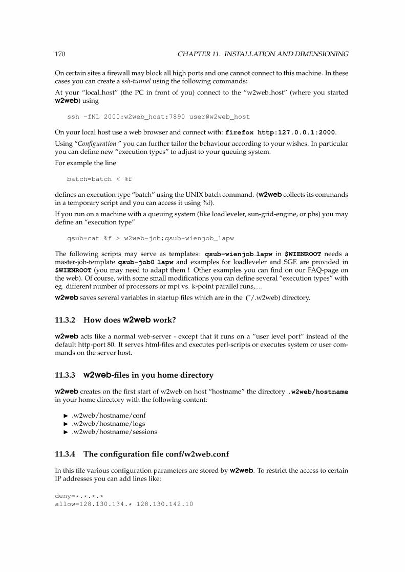
170 CHAPTER 11. INSTALLATION AND DIMENSIONING
On certain sites a firewall may block all high ports and one cannot connect to this machine. In thesecases you can create a ssh-tunnel using the following commands:
At your “local host” (the PC in front of you) connect to the “w2web host” (where you startedw2web) using
ssh -fNL 2000:w2web_host:7890 user@w2web_host
On your local host use a web browser and connect with: firefox http:127.0.0.1:2000.
Using “Configuration ” you can further tailor the behaviour according to your wishes. In particularyou can define new “execution types” to adjust to your queuing system.
For example the line
batch=batch < %f
defines an execution type “batch” using the UNIX batch command. (w2web collects its commandsin a temporary script and you can access it using %f).
If you run on a machine with a queuing system (like loadleveler, sun-grid-engine, or pbs) you maydefine an “execution type”
qsub=cat %f > w2web-job;qsub-wienjob_lapw
The following scripts may serve as templates: qsub-wienjob lapw in $WIENROOT needs amaster-job-template qsub-job0 lapw and examples for loadleveler and SGE are provided in$WIENROOT (you may need to adapt them ! Other examples you can find on our FAQ-page onthe web). Of course, with some small modifications you can define several “execution types” witheg. different number of processors or mpi vs. k-point parallel runs,....
w2web saves several variables in startup files which are in the (˜/.w2web) directory.
11.3.2 How does w2web work?
w2web acts like a normal web-server - except that it runs on a ”user level port” instead of thedefault http-port 80. It serves html-files and executes perl-scripts or executes system or user com-mands on the server host.
11.3.3 w2web-files in you home directory
w2web creates on the first start of w2web on host “hostname” the directory .w2web/hostnamein your home directory with the following content:
I .w2web/hostname/confI .w2web/hostname/logsI .w2web/hostname/sessions
11.3.4 The configuration file conf/w2web.conf
In this file various configuration parameters are stored by w2web. To restrict the access to certainIP addresses you can add lines like:
deny=*.*.*.*allow=128.130.134.* 128.130.142.10

11.4. ENVIRONMENT VARIABLES 171
11.3.5 The password file conf/w2web.users
This file is created during the first run of w2web.
If you remove this file, the next start of w2webwill activate the installation procedure again.
11.3.6 Using the https-protocol with w2web
In order to use the https-protocol the perl-library Net::SSLeay in addition to the OpenSSL packagemust be installed on your system. Both are freely available.
Then you must include a line with ssl=1 in w2web.conf.
If you run w2web-server in ssl-mode you need a site certificate for your server. You may usethe supplied certificate in $WIENROOT/SRC w2web/bin/w2web.pem (copy this file to your conf-directory and set the keyfile= /.w2web/¡hostname¿/conf/w2web.pem line in your w2web.conf).
This certificate will not expire until 2015, but usually browsers will complain that they do not knowthe Certificate Authority who issued this certificate - if you don’t like this message, you must buya certificate from VeriSign, Thawte or a similar CA.
Of course you must connect to https: instead of http:, i.e. use:
netscape https://hostname where w2web runs:7890.
11.4 Environment Variables
WIEN2k uses the following environment variables:
WIENROOT base directory where WIEN2k is installedPDFREADER specifies program to read pdf files (acroread, xpdf,...)SCRATCH directory where case.vector and case.help?? are stored.EDITOR path and name of your prefered editorSTRUCTEDIT PATH path where the structeditor tool is locatedOCTAVE PATH path where the structeditor tool is locatedOCTAVE EXEC PATH path where octave looks for executables (structeditor)XCRYSDEN TOPDIR if this variable is set WIEN2k will activate all interface extensions to XCrys-
Den.USE REMOTE [0|1] determines whether parallel jobs are run in background (on shared memory
machines) or using rsh. It is overridden by settings in $WIENROOT/parallel optionsWIEN GRANULARITY Default granularity for parallel execution. It is overridden by setting the
granularity in the .machines file or in $WIENROOT/parallel optionsWIEN EXTRAFINE if set, the residual k-points are spread one by one over the processors.
In addition on some systems variables like:
LD LIBRARY PATH path to libraries of compiler and math-libsOMP NUM THREADS on multi-core machines for parallelization in certain libraries (mkl, goto)

172 CHAPTER 11. INSTALLATION AND DIMENSIONING

12 Trouble shooting
In this chapter hints are given for solving some difficulties that have occurred frequently. Thischapter is by no means complete and the authors would appreciate further suggestions whichmight be useful for other users. Beside the printed version of the users guide, an online pdf ver-sion is available using help lapw. You can search for a specific keyword (use ∧f keyword) andhopefully find some information.
There is a mailing list for WIEN2k related questions. To subscribeto this list send mail to:[email protected] the text “subscribe wien”. You will then automatically beadded to the mailing [email protected] make use of this list!
If an error occurs in one of the SCF programs, a file program.error is created and an error messageis printed into these files. The run lapw script checks for these files and will automatically stop ifa non-empty error file occurs.
Check the files case.dayfile (which is written by init lapw and run lapw), :log (where ahistory of all commands using x is given) and *.error for possible explanations.
In several places the dimensions are checked. The programs print a descriptive error message andstop.
case.outputnn: This file gives error messages if the atomic spheres overlap. But it should alsobe used to check the distances between the atoms and the coordination number (same dis-tance). If inconsistencies exists, your case.struct file may contain an error. A check foroverlapping spheres is also included in mixer and lapw1.
case.outputd: Possible stops or warnings are:“NO SYMMETRY OPERATION FOUND IN ROTDEF“: This indicates that in your
case.struct file either the positions of equivalent atoms are not specified correctly(only positive coordinates allowed!!) or the symmetry operations are wrong.
case.output1: Possible stops or warnings are:“NO ENERGY LIMITS FOUND IN SELECT“: This indicates that Etop or Ebottom could not
be found for some ul(r, El). Check your input if it happens in the zeroth iteration. Later,(usually in the second to sixth iteration) it may indicate that in your SCF cycle some-thing went wrong and you are using a crazy potential. Usually it means that mixingwas too big and large charge fluctuations occured. Check previous charges for beingphysically reasonable (grep for labels :NTOxx :CTOxx :DIS). You will probably have todelete case.broy* and case.scf, rerun x dstart and reduce the mixing parameterin case.inm. In very difficult (magnetic) cases a PRATT mixing with 0.01 mixing mightbe necessary at the beginning!
173

174 CHAPTER 12. TROUBLE SHOOTING
“STOP RDC 22“: This indicates that the overlap matrix is not positive definite. This usuallyhappens if your case.struct file has some error in the structure or if you have an(almost) linear dependent basis, which can happen for large RKMAX values and/or ifyou are using very different (extremely small and large) sphere radii RMT .
“X EIGENVALUES BELOW THE ENERGY emin“: This indicates that X eigenvalues werefound below emin. Emin is set in case.in1 (see sec. 7.3.3) or in case.klist gener-ated by KGEN, see 6.3, 6.5). It may indicate that your value of emin is too high or thepossibility of ghostbands, but it can also be intentional to truncate some of the low lyingeigenvalues.
If you don’t find enough eigenvalues (e.g.: in a cell with 4 oxygens you expect 4 oxygen sbands at roughly -1 Ry) check the energy window (given at the end of the first k-pointin case.in1 or in case.klist) and make sure your energy parameters are found bysubroutine SELECT or set them by hand at a reasonable value.
case.output2: Possible stops or warnings are:
“CANNOT BE FOUND“: This warning, which could produce a very long output file, in-dicates that some reciprocal K-vector would be requested (through the k-vector list oflapw1), but was not present in the list of the K generated in lapw2. You may haveto increase the NWAV, and/or KMAXx parameters in lapw2 or increase GMAX incase.in2. The problems could also arise from wrong symmetry operations or a wrongstructure in case.struct.
“QTL-B VALUE“: If larger than a few percent, this indicates the appearance of ghost bands,which are discussed below in section 12.1.The few percent message (e.g up to 10 %) does not indicate a ghost band, but can happene.g. in narrow d-bands, where the linearization reaches its limits. In these cases one canadd a local orbital to improve the flexibility of the basis set. (Put one energy near the topand the other near the bottom of the valence band, see section 7.3.3).
FERMI LEVEL not converged (or similar messages). This can have several reasons: i) Try adifferent Fermi-Method (change TETRA to GAUSS or TEMP in case.in2). ii) Countthe number of eigenvalues in case.output1 and compare it with the number of va-lence electrons. If there are too few eigenvalues, either increase EMAX in case.klist(from 1.5 to e.g. 2.5) or check if your scf cycle had large charge oszillations (see SELECTerror above)
If the SCF cycle stops somewhere (especially in the first few iterations), it is quite possible, thatthe source of the error is actually in a previous part of the cycle or even in a previous (e.g. thezeroth) iteration. Check in the case.scf file previous charges, eigenvalues, . . . whether they arephysically reasonable (see SELECT error above).
12.1 Ghost bands
Approximate linear dependence of the basis set or the linearization of the energy dependence ofthe radial wave functions (see section 2.2) can lead to spurious eigenvalues, termed “ghost bands”.
The first case may occur in a system which has atoms with very different atomic sphere radii.Suppose you calculate a hydroxide with very short O-H bonds so that you select small RMT radiifor O and H such as e.g. 1.0 and 0.6 a.u., respectively. The cation may be large and thus youcould choose a large RMT of e.g. 2.4 a.u. However, this gives a four time larger effective RKmaxfor the cation than for H, (e.g. 16.0 when you select RKmax=4.0 in case.in1). This enormousdifference in the convergence may lead to unphysical eigenvalues. In such cases choose lmax=12in case.in1 (in order to get a very good re-expansion of the plane waves) and reduce RMT forthe cation to e.g. 1.8 a.u.

12.1. GHOST BANDS 175
The second case can occur when you don’t use a proper set of local orbitals. In this situation theenergy region of interest (valence bands) falls about midway between two states with differentprinciple quantum numbers, but with the same l-value (for one atom).
Take for example Ti with its 3p states being occupied as (semi-core) states, while the 4p states remainmostly unoccupied. In the valence band region neither of those two states (Ti 3p, 4p) should appear.If one uses 0.2 Ry for the expansion energy E(1) for the p states of Ti, then Ti-p states do appear asghost bands. Such a run is shown below for TiO2 (rutile).
The lowest six eigenvalues at GAMMA fall between about -1.30 and -1.28 Ry. They are ghost bandsderived from fictitious Ti-p states. The next four eigenvalues between -0.94 and -0.78 Ry correspondto states derived from O 2s states, which are ok, since there are four O’s per unit cell, four statesare found.
The occurrence of such unphysical (indeed, unchemical!) ghostbands is the first warning thatsomething went wrong. A more definite warning comes upon running LAPW2, where the corre-sponding charge densities are calculated. If the contribution to the charge density from the energyderivative of the basis function [the Blm coefficient in equ. 2.4,2.7] is significant (i.e. much morethan 5 per cent) then a warning is issued in LAPW2.
In the present example it reads:
QTL-B VALUE .EQ. 40.35396 !!!!!!
This message is found in both the case.scf file and in case.output2.
When such a message appears, one can also look at the partial charges (QTL), which are printedunder these conditions to OUTPUT2, and always appear in the files case.helpXXX, etc., wherethe last digit refers to the atomic index.
In the file below, note the E(1) energy parameter as well as the 6 ghost band energies around -1.29.
--------------- top of file:tio2.scf -----------------------------ATOMIC SPHERE DEPENDENT PARAMETERS FOR ATOM TitaniumOVERALL ENERGY PARAMETER IS .2000E( 0)= .2000
---> E( 1)= .2000E( 2)= .2000 E(BOTTOM)= -.140 E(TOP)= -200.000
ATOMIC SPHERE DEPENDENT PARAMETERS FOR ATOM OxygenOVERALL ENERGY PARAMETER IS .2000E( 0)= -.7100 E(BOTTOM)= -2.090 E(TOP)= .670
K= .00000 .00000 .00000 1:RKM : MATRIX SIZE= 599 RKM= 6.99 WEIGHT= 8.00 PGR:
EIGENVALUES ARE:-1.2970782 -1.2970782 -1.2948747 -1.2897193 -1.2897193-1.2882306 -.9389111 -.8484857 -.7880729 -.7880729-.0484830 -.0162982 .0121181 .0976534 .0976534.1914068 .1914068 .2341991 .3286919 .3477629.3477629 .3809219 .5143729 .5356211 .5550735.5617155 .5617155 .7087550 .7197110 .8736991.8736991 .9428865 .9533619 1.2224570 1.2224570
1.4285169
********************************************************NUMBER OF K-POINTS: 1
:NOE : NUMBER OF ELECTRONS = 48.000:FER : F E R M I - ENERGY = .53562
:POS01: AT.NR. -1 POSITION = .00000 .00000 .00000 MULTIPLICITY= 2LMMAX=10LM= 0 0 2 0 2 2 4 0 4 2 4 4 6 0 6 2 6 4 6 6 0 0 0 0 0 0 0 0 0 0 0 0 0 0
:CHA01: TOTAL CHARGE INSIDE SPHERE 1 = 8.802166:PCS01: PARTIAL CHARGES SPHERE = 1 S,P,D,F,PX,PY,PZ,D-Z2,D-X2Y2,D-XY,D-XZ,D-YZ:QTL01: .127 6.080 2.518 .067 2.011 2.047 2.022 1.090 .760 .155 .480 .034
VXX VYY VZZ UP TO R:VZZ01: -4.96856 8.48379 -3.51524 2.000

176 CHAPTER 12. TROUBLE SHOOTING
:POS02: AT.NR. -2 POSITION = .30500 .30500 .00000 MULTIPLICITY= 4LMMAX=16LM= 0 0 1 0 2 0 2 2 3 0 3 2 4 0 4 2 4 4 5 0 5 2 5 4 6 0 6 2 6 4 6 6 0 0
:CHA02: TOTAL CHARGE INSIDE SPHERE 2 = 5.486185:PCS02: PARTIAL CHARGES SPHERE = 2 S,P,D,F,PX,PY,PZ,D-Z2,D-X2Y2,D-XY,D-XZ,D-YZ:QTL02: 1.559 3.902 .022 .002 1.296 1.306 1.300 .014 .004 .000 .003 .001
VXX VYY VZZ UP TO R:VZZ02: .25199 -.55091 .29892 1.600
:CHA : TOTAL CHARGE INSIDE CELL = 48.000000:SUM : SUM OF EIGENVALUES = -15.810906
QTL-B VALUE .EQ. 40.35396 !!!!!!NBAND in QTL-file: 24
----------------end of truncated file tio2.scf----------------------
Next we show tio2.output2 for the first of the ghost bands at -1.297 Ry. One sees that it corre-sponds mainly to a p-like charge, which originates from the energy derivative part Q(UE) of theKohn-Sham orbital. Q(UE) contributes 40.1% compared with 8.5% from the main component Q(U).Q(UE) greater than Q(U) is a good indication for a ghost band.
----------------part of file tio2.output2 --------------------------QTL-B VALUE .EQ. 40.35396 !!!!!!
K-POINT: .0000 .0000 .0000 599 36 1BAND # 1 E= -1.29708 WEIGHT= 2.0000000
L= 0 L= 1 PX: PY: PZ: L= 2 DZ2: DX2Y2: DXY: DXZ: DYZ: L= 3QINSID: .0000 48.6035 35.0996 13.5039 .0000 .0000 .0000 .0000 .0000 .0000 .0000 .0030Q(U) : .0000 8.4902 6.0125 2.4777 .0000 .0000 .0000 .0000 .0000 .0000 .0000 .0026Q(UE) : .0000 40.1132 29.0871 11.0261 .0000 .0000 .0000 .0000 .0000 .0000 .0000 .0005
L= 0 L= 1 PX: PY: PZ: L= 2 DZ2: DX2Y2: DXY: DXZ: DYZ: L= 3QINSID: .1294 .0707 .0000 .0055 .0653 .0088 .0038 .0049 .0000 .0000 .0000 .0022Q(U) : .1279 .0627 .0000 .0052 .0575 .0087 .0038 .0049 .0000 .0000 .0000 .0020Q(UE) : .0016 .0081 .0000 .0003 .0077 .0001 .0000 .0000 .0000 .0000 .0000 .0002QOUT : 1.9265
----------------------bottom of truncated file ----------------------
Another file in which the same information can be found is tio2.help031, since the ghost bandis caused by a bad choice for the Ti-p energy parameter:
----------------------Top of file tio2.help031 ---------------------K-POINT: .0000 .0000 .0000 599 36 1BAND # 1 E= -1.29708 WEIGHT= 2.0000000L= 0 .00000 .00000 .00000 .00000 .00000 .00000L= 1 48.60346 8.49022 40.11324 .00000 .00000 .00000
PX: 35.09960 6.01247 29.08712 .00000 .00000 .00000PY: 13.50386 2.47774 11.02612 .00000 .00000 .00000PZ: .00000 .00000 .00000 .00000 .00000 .00000
L= 2 .00000 .00000 .00000 .00000 .00000 .00000DZ2: .00000 .00000 .00000 .00000 .00000 .00000
DX2Y2: .00000 .00000 .00000 .00000 .00000 .00000DXY: .00000 .00000 .00000 .00000 .00000 .00000DXZ: .00000 .00000 .00000 .00000 .00000 .00000DYZ: .00000 .00000 .00000 .00000 .00000 .00000
L= 3 .00304 .00255 .00050 .00000 .00000 .00000L= 4 .00000 .00000 .00000 .00000 .00000 .00000L= 5 .00096 .00082 .00014 .00000 .00000 .00000L= 6 .00000 .00000 .00000 .00000 .00000 .00000
-------------------bottom of truncated file--------------------------
Note again for L=1 the percentage of charge associated with the primary (APW) basis functions ul(8.5%) versus that coming from the energy derivative component (40.1%).
If a ghost band appears, one should first analyze its origin as indicated above, then use appropriatelocal orbitals to improve the calculation and get rid of these unphysical states.
Do not perform calculations with “ghost-bands”, even when the calculation converges.
Good luck !

13 References
Abt R., Ambrosch-Draxl C. and Knoll P. 1994 Physica B 194-196
Abt R. 1997 PhD Theses, Univ.Graz
Andersen O.K. 1973 Solid State Commun. 13, 133
— 1975 Phys. Rev. B 12, 3060
Ambrosch-Draxl C., Blaha P., and Schwarz K. 1991 Phys.Rev. B44, 5141
Ambrosch-Draxl C., Majewski J. A., Vogl P., and Leising G. 1995, PRB 51 9668
Ambrosch-Draxl C. and Sofo J., 2006 Comp. Phys. Comm. 175, 1
V.I. Anisimov, I.V. Solovyev, M.A. Korotin, M.T. Czyzyk, and G.A. Sawatzky, Phys. Rev. B 48,16929 (1993).
V.I. Anisimov, J. Zaanen, and O.K. Andersen, Phys. Rev. B 44, 943 (1991)
Bader R. F. W. 2001: http://www.chemistry.mcmaster.ca/faculty/bader/aim/
Blaha P. and Schwarz K. 1983 Int. J. Quantum Chem. XXIII, 1535
Blaha P., Schwarz K., and Herzig P 1985 Phys. Rev. Lett. 54, 1192
Blaha P., Schwarz K., and Dederichs P 1988 Phys. Rev B 38, 9368
Blaha P., Schwarz K., Sorantin P.I. and Trickey S.B. 1990 Comp. Phys. Commun. 59, 399
Blaha P., Sorantin P.I., Schwarz K and Singh D. 1992 Phys. Rev. B 46, 1321
Blochl P.E., Jepsen O. and Andersen O.K. 1994, Phys. Rev B 49, 16223
Boettger J.C. and Albers R.C. 1989 Phys. Rev. B 39, 3010
Boettger J.C. and Trickey S.B. 1984 Phys. Rev. B 29, 6425
Brooks M.S.S. 1985 Physica B 130, 6
Charpin, T. 2001. (see $WIENROOT/SRC/elast-UG.ps)
Czyzyk M.T. and G.A. Sawatzky, Phys. Rev. B 49, 14211 (1994).
Desclaux J.P. 1969 Comp. Phys. Commun. 1, 216; note that the actual code we use is an ap-parently unpublished relativistic version of the non-relativistic code described in this paper.Though this code is widely circulated, we have been unable to find a formal reference for it.
— 1975 Comp. Phys. Commun. 9, 31; this paper contains much of the Dirac-Fock treatmentused in Desclaux’s relativistic LSDA code.
177

178 CHAPTER 13. REFERENCES
O. Eriksson, B. Johansson, and M.S.S. Brooks, J. Phys. C 1, 4005 (1989)
Feldman J.L., Mehl M.J., and Krakauer H. 1987 Phys. Rev. B 35, 6395
Gay David M., ”ALGORITHM 611 – Subroutines for Unconstrained Minimization Using aModel/Trust-Region Approach”, ACM Trans. Math. Software 9 (1983), pp. 503-524.
Hebert-Souche C., Louf P.-H., Blaha P., M. Nelhiebel, Luitz J., Schattschneider P., SchwarzK. and Jouffrey B.; The orientation dependent simulation of ELNES, Ultramicroscopy, 83, 9(2000)
L.L. Hirst, Rev. Mod. Phys. 69, 607 (1997)
Hohenberg P. and Kohn W. 1964 Phys. Rev. 136, B864
Hofstatter H., Koch R., Laskowski R., Blaha P. and Schwarz K., to be published (2008)
“International Tables for X-Ray Crystallography“ 1964 Vol.1; The Kynoch Press, BirminghamUK
Jansen H.J.F. and Freeman A.J. 1984 Phys. Rev. B 30, 561
— 1986 Phys. Rev. B 33, 8629
Koelling D.D. 1972 J. Phys. Chem. Solids 33, 1335
Koelling D.D. and Arbman G.O. 1975 J.Phys. F: Met. Phys. 5, 2041
Koelling D.D. and Harmon B.N. 1977 J. Phys. C: Sol. St. Phys. 10, 3107
Kohler B., Wilke S., Scheffler M., Kouba R. and Ambrosch-Draxl C. 1996Comp.Phys.Commun. 94, 31
Kohn W. and Sham L.J. 1965 Phys. Rev. 140, A1133
Kokalj A. 1999 J.Mol.Graphics and Modelling 17, 176
Krimmel H.G., Ehmann J., Elsasser C., Fahnle M. and Soler J.M. 1994, Phys.Rev. B50, 8846
Kunes J, Novak P., Schmid R., Blaha P. and Schwarz K. 2001, Phys. Rev. B64, 153102
Kara, M. and Kurki-Suonio K. 1981 Acta Cryst A37, 201
Liberman D., Waber J.T., and Cromer D.T. 1965, Phys. Rev. 137A, 27
A.I. Liechtenstein, V. I. Anisimov, J. Zaanen, Phys. Rev. B 52, R5467 (1995)
Luitz J., Maier M., Hebert C., Schattschneider P., Blaha P., Schwarz K., Jouffrey B. 2001 Eur.Phys J. B 21, 363-367
MacDonald A. H., Pickett, W. E. and Koelling, D. D. 1980 J. Phys. C 13, 2675
Madsen G. K. H., Blaha P, Schwarz K, Sjostedt E and Nordstrom L 2001, Phys. Rev. B64,195134
Marks L. D., and Luke R. 2008, Phys. Rev. B 78, 075114
Mattheiss L.F. and Hamann D.R. 1986 Phys. Rev. B 33, 823
Mattsson A., Armiento R., Paier J., Kresse G., Wills J. and Mattsson T 2008 J. Chem. Phys.128, 084714
Meyer-ter-Vehn J. and Zittel W. 1988 Phys. Rev. B37, 8674

179
Moruzzi V.L., Janak J.F., and Williams A.R. 1978 “Calculated Properties of Metals“ (Perga-mon, NY)
Murnaghan F.D., Proc.Natl.Acad.Sci. USA 30, 244 (1944)
Neckel A., Schwarz K., Eibler R. and Rastl P. 1975 Microchim.Acta, Suppl.6, 257
Nelhiebel M., Louf P. H., Schattschneider P., Blaha P., Schwarz K. and Jouffrey B.; Theory oforientation sensitive near-edge fine structure core-level spectroscopy, Phys.Rev. B59, 12807(1999)
Novak P. 1997 see $WIENROOT/SRC/novak lecture on spinorbit.ps
Novak P. , Boucher F., Gressier P., Blaha P. and Schwarz K. 2001 Phys. Rev. B 63, 235114
Novak P. 2001 see $WIENROOT/SRC/novak lecture on ldaumatrixelements.ps andhttp://www.wien2k.at/reg user/textbooks
Novak P. 2006 see $WIENROOT/SRC/Bhf 3.ps and http://www.wien2k.at/reg user/textbooks
Perdew J.P, Chevary J.A., Vosko S.H., Jackson K.A., Pederson M.R., Singh D.J., and FiolhaisC. 1992 Phys.Rev.B46, 6671
Perdew J.P. and Wang Y. 1992, Phys.Rev. B45, 13244
Perdew J.P., Burke S. and Ernzerhof M. 1996, Phys.Rev.Let. 77, 3865
Perdew J.P., Kurth S., Zupan J. and Blaha P. 1999, Phys.Rev.Let. 82, 2544
Perdew J.P. et al. 2008, Phys. Rev. Let. 100, 136406
Pratt G.W. 1952 Phys. Rev. 88, 1217
Ray A.K. and Trickey S.B. 1981 Phys. Rev. B24, 1751; erratum 1983, Phys. Rev. B28, 7352
Rondinelli JM, Beng Bin and Marks LD. 2007, Comp. Mater. Sci. 40, 345-353 (also: LosAlamos archive, physics/0608160 (http://xxx.lanl.gov/abs/physics/0608160)
Schwarz K., Neckel A and Nordgren J, J.Phys.F:Metal Phys. 9, 2509 (1979)
Schwarz K., and Wimmer E, J.Phys.F:Metal Phys. 10, 1001 (1980)
Schwarz K. and Blaha P.: Lecture Notes in Chemistry 67, 139 (1996)
Schwarz K., P.Blaha and Madsen, G. K. H. Comp.Phys.Commun. 147, 71 (2002)
Singh D., Krakauer H., and Wang C.-S. 1986 Phys. Rev. B34, 8391
Singh, D. 1989 Phys. Rev. B40, 5428
Singh D. 1991, Phys.Rev. B43, 6388
Singh D. 1994, Plane waves, pseudopotentials and the LAPW method, Kluwer Academic
Sjostedt E, Nordstrom L and Singh D. J. 2000 Solid State Commun. 114, 15
Sofo J and Fuhr J 2001: $WIENROOT/SRC/aim sofo notes.ps
Soler J.M. and Williams A.R. 1989, Phys.Rev. B40, 1560
Sorantin P.I., and Schwarz K.H. 1992, Inorg.Chem. 31, 567
Stahn J, Pietsch U, Blaha P and Schwarz K. 2001, Phys.Rev. B63, 165205

180 CHAPTER 13. REFERENCES
Tao Jianmin, Perdew J.P., Staroverov V. and Scuseria G. 2003, Phys.Rev.Let. 91, 146401
Tran F, Laskowski R, Blaha P and Schwarz K. 2007, Phys. Rev. B 75, 115131
Tran F, Blaha P Schwarz K and Novak P 2006, Phys. Rev. B 74, 155108
von Barth U. and Hedin L. 1972 J. Phys. C.: Sol. St. Phys. 5, 1629
Wei S.H., Krakauer H., and Weinert M. 1985 Phys. Rev. B 32, 7792
Weinert M. 1981 J. Math. Phys. 22, 2433
Weinert M., Wimmer E., and Freeman A.J. 1982 Phys. Rev. B26, 4571
Wimmer E., Krakauer H., Weinert M., and Freeman A.J. 1981 Phys. Rev. B24, 864
Wu Z., Cohen R., 2006 Phys. Rev. B73, 235116
Yanchitsky B. and Timoshevskii T. 2001, Comp.Phys.Commun. 139, 235
Yu R., Singh D. and Krakauer H. 1991, Phys.Rev. B43, 6411

Part IV
Appendix
181


A Local rotation matrices
Local rotation matrices are used to rotate the global coordinate system (given by the definition ofthe Bravais matrix) to a local coordinate system for each atomic site. They are used in the programfor two reasons:
I to minimize the number of LM combinations in the lattice harmonics expansion (of potentialand charge density according to equ. 2.10). For example for point group mm2 one needs forL=1 just LM=1,0 if the coordinate system is chosen such that the z-axis coincides with the2-fold rotation axis, while in an arbitrary coordinate system the three terms 1,0; 1,1 and -1,1are needed (and so on for higher L).
I The interpretation e.g. of the partial charges requires a proper orientation of the coordinatesystem. In the example given above, the p orbitals split into 2 irreducible representations, butthey can be attributed to pz and px, py only if the z-axis is the 2-fold rotation axis.
It is of course possible to perform calculations without “local rotation matrices“, but in such a casethe LM combinations given in Table 7.42 (and by SYMMETRY) may not be correct. (The LM valuesfor arbitrary orientations may be obtained from a procedure described in Singh 94.)
Fortunately, the “local rotation matrices“ are usually fairly simple and are now automatically in-serted into your case.struct file. Nevertheless we recommend to check them in order to besure.
The most common coordinate transformations are
I interchanging of two axes (e.g. x and z)I rotation by 45 (e.g. in the xy-plane)I rotation of z into the (111) direction
Inspection of the output of SYMMETRY tells you if the local rotation matrix is the unit matrix or itgives you a clear indication how to find the proper matrix.
The local rotation matrix R , which transforms the global coordinates r to the rotated ones r′, isdefined by Rr = r′.
There are two simple ways to check the local rotation matrixes together with the selected LM com-binations:
I charge density plots generated with LAPW5 must be continuous across the atomic sphereboundary (especially valence or difference density plots are very sensitive, see 8.6)
I Perform a run of LAPW1 and LAPW2 using the GAMMA-point only (or a complete star ofanother k point). In such a case, “wrong“ LM combinations must vanish. Note that the latteris true only in this case. For a k mesh in the IBZ “wrong“ LM combinations do not vanishand thus must be omitted!!
A first example for “local rotation matrices“ is given for the rutile TiO2, which has already beendescribed as an example in section 10.3. Also two other examples will be given (see below).
183

184 APPENDIX A. LOCAL ROTATION MATRICES
A.1 Rutile (TiO2)
Examine the output from symmetry. It should be obvious that you need local rotation matrices forboth, Ti and O:
....Titanium operation # 1 1Titanium operation # 2 -1Titanium operation # 5 2 || zTitanium operation # 6 m n zTitanium operation # 12 m n 110Titanium operation # 13 m n -110Titanium operation # 18 2 || 110Titanium operation # 19 2 || -110pointgroup is mmm (neg. iatnr!!)axes should be: m n z, m n y, m n x
This output tells you, that for Ti a mirror plan normal to z is present, but the mirror planes normalto x and y are missing. Instead, they are normal to the (110) plane and thus you need to rotate x, yby 45 around the z axis. (The required choice of the coordinate system for mmm symmetry is alsogiven in Table 7.42)
....Oxygen operation # 1 1Oxygen operation # 6 m n zOxygen operation # 13 m n -110Oxygen operation # 18 2 || 110pointgroup is mm2 (neg. iatnr!!)axes should be: 2 || z, m n y
For O the 2-fold symmetry axes points into the (110) direction instead of z. The appropriate rotationmatrices for Ti and O are: 1√
21√2
0−1√
21√2
00 0 1
0 −1√2
1√2
0 1√2
1√2
1 0 0
A.2 Si Γ-phonon
Si possesses a face-centered cubic structure with two equivalent atoms per unit cell, at (±0.125,±0.125, ±0.125). The site symmetry is -43m. For the Γ-phnon the two atoms are displaced inopposite direction along the (111) direction and cubic symmetry is lost. The output of SYMMETRYgives the following information:
Si operation # 1 1Si operation # 13 m n -110Si operation # 16 m n -101Si operation # 17 m n 0-11Si operation # 24 3 || 111Si operation # 38 3 || 111pointgroup is 3m (neg. iatnr!!)
axis should be: 3 || z, m n ylm: 0 0 1 0 2 0 3 0 3 3 4 0 4 3 5 0 5 3 6 0 6 3 6

A.3. TRIGONAL SELENIUM 185
Therefore the required local rotation matrix should rotate z into the (111) direction and thus thematrix in the “struct“ file should be:
0.4082483 -.7071068 0.5773503√
66 −
√2
2
√3
3
0.4082483 0.7071068 0.5773503√
66
√2
2
√3
3
-.8164966 0.0000000 0.5773503 −2√
66
√2
2
√3
3
A.3 Trigonal Selenium
Selenium possesses space group P3121 with the following struct file:
H LATTICE,NONEQUIV.ATOMS: 1MODE OF CALC=RELA POINTGROUP:328.2500000 8.2500000 9.369000
ATOM= -1: X= .7746000 Y= .7746000 Z= 0.0000000MULT= 3 ISPLIT= 8
ATOM= -1: X= .2254000 Y= .0000000 Z= 0.3333333ATOM= -1: X= .0000000 Y= .2254000 Z= 0.6666667Se NPT= 381 R0=.000100000 RMT=2.100000000 Z:34.0LOCAL ROT.MATRIX: 0.0 0.5000000 0.8660254
0.0000000 -.8660254 0.50000001.0000000 0.0000000 0.0
6 IORD OF GROUP G0......
The output of SYMMETRY reads:
Se operation # 1 1Se operation # 9 2 $|$$|$ 110pointgroup is 2 (neg. iatnr!!)axis should be: 2 || z
lm: 0 0 1 0 2 0 2 2 -2 2 3 0 3 2 -3 2 4 0 4 2 -4 2 ......
Point group 2 should have its 2-fold rotation axis along z, so the local rotation matrix can be con-structed in two steps: firstly interchange x and z (that leads to z ‖ (011) ) and secondly rotate from(011) into (001) (see the struct file given above). Since this is a hexagonal lattice, SYMMETRY usesthe hexagonal axes, but the local rotation matrix must be given in cartesian coordinates.

186 APPENDIX A. LOCAL ROTATION MATRICES

B Periodic Table
187

188 APPENDIX B. PERIODIC TABLE
Per
iodi
c T
able
of
the
Ele
men
ts
1 H 1s
2 He
1s2
3 Li
He2
s
4 Be
He2
s2
5 BH
e2s2 2p
6 CH
e2s2 2p
2
7 NH
e2s2 2p
3
8 OH
e2s2 2p
4
9 FH
e2s2 2p
5
10N
eH
e2s2 2p
6
11N
aN
e3s
12M
gN
e3s2
13A
lN
e3s2 3p
14Si
Ne3
s2 3p2
15P
Ne3
s2 3p3
16S
Ne3
s2 3p4
17C
lN
e3s2 3p
5
18A
rN
e3s2 3p
6
19K
Ar4
s
20C
aA
r4s2
21Sc
Ar3
d1 4s2
22T
iA
r3d2 4s
2
23V
Ar3
d3 4s2
24C
rA
r3d5 4s
1
25M
nA
r3d5 4s
2
26F
eA
r3d6 4s
2
27C
oA
r3d7 4s
2
28N
iA
r3d8 4s
2
29C
uA
r3d10
4s1
30Z
nA
r3d10
4s2
31G
aA
r3d10
4s2 4p
32G
eA
r3d10
4s2 4p
2
33A
sA
r3d10
4s2 4p
3
34Se
Ar3
d104s
2 4p4
35B
rA
r3d10
4s2 4p
5
36K
rA
r3d10
4s2 4p
6
37R
bK
r5s
38Sr
Kr5
s2
39Y
Kr4
d1 5s2
40Z
rK
r4d2 5s
2
41N
bK
r4d3 5s
2
42M
oK
r4d5 5s
1
43T
cK
r4d5 5s
2
44R
uK
r4d6 5s
2
45R
hK
r4d7 5s
2
46P
dK
r4d8 5s
2
47A
gK
r4d10
5s1
48C
dK
r4d10
5s2
49In
Kr4
d105s
2 5p
50Sn
Kr4
d105s
2 5p2
51Sb
Kr4
d105s
2 5p3
52T
eK
r3d10
5s2 5p
4
53I
Kr4
d105s
2 5p5
54X
eK
r4d10
5s2 5p
6
55C
sX
e6s
56B
aX
e6s2
57-7
1
La-
Lu
72H
fX
e4f14
5d2 6s
2
73T
aX
e4f14
5d3 6s
2
74W
Xe4
f145d
5 6s1
75R
eX
e4f14
5d5 6s
2
76O
sX
e4f14
5d6 6s
2
77Ir
Xe4
f145d
7 6s2
78P
tX
e4f14
5d8 6s
2
79A
uX
e4f14
5d10
6s1
80H
gX
e4f14
5d10
6s2
81T
lX
e4f14
5d10
6s2 6p
82P
bX
e4f14
5d10
6s2 6p
2
83B
iX
e4f14
5d10
6s2 6p
3
84P
oX
e4f14
3d10
6s2 6p
4
85A
tX
e4f14
5d10
6s2 6p
5
86R
nX
e4f14
5d10
6s2 6p
6
87F
rR
n7s
88R
aR
n7s2
89-1
03
Ac-
Lr
57L
aX
e5d6
s2
58C
eX
e4f2 6s
2
59P
rX
e4f3 6s
2
60N
dX
e4f4 6s
2
61P
mX
e4f5 6s
2
62Sm
Xe4
f6 6s2
63E
uX
e4f7 6s
2
64G
dX
e4f7 5d
6s2
65T
bX
e4f9 6s
2
66D
yX
e4f10
6s2
67H
oX
e4f11
6s2
68E
rX
e4f12
6s2
69T
mX
e4f13
6s2
70Y
bX
e4f14
6s2
71L
uX
e4f14
5d6s
2
89A
cR
n6d7
s2
90T
hR
n6d2 7s
2
91P
aR
n5f2 6d
1 7s2
92U
Rn5
f3 6d1 7s
2
93N
pR
n5f4 6d
1 7s2
94P
uR
n5f6 7s
2
95A
mR
n5f7 7s
2
96C
mR
n5f7 6d
7s2
97B
kR
n5f9 7s
2
98C
fR
n5f10
7s2
99E
sR
n5f11
7s2
100 F
mR
n5f12
7s2
101 M
dR
n5f13
7s2
102 N
oR
n5f14
7s2
103 L
rR
n5f14
6d7s
2


WIEN2kISBN 3-9501031-1-2


