Embed Size (px)
Citation preview
WIDER Working Paper 2017/94
Cognitive, socioemotional, and behavioural returns to college quality
Utteeyo Dasgupta,1 Subha Mani,2 Smriti Sharma,3 Saurabh Singhal4
April 2017
1 Department of Economics, Wagner College, and Center for International Policy Studies, Fordham University, NY, USA, [email protected]; 2 Department of Economics and Center for International Policy Studies, Fordham University, NY, USA; Population Studies Center, University of Pennsylvania, PA, USA, and IZA, Bonn, Germany, corresponding author: [email protected]; 3 UNU-WIDER, Helsinki, Finland, [email protected]; 4 UNU-WIDER, Helsinki, Finland, [email protected]
This study has been prepared within the UNU-WIDER project on ‘Inequality in the giants’.
Copyright © UNU-WIDER 2017
Information and requests: [email protected]
ISSN 1798-7237 ISBN 978-92-9256-318-9
Typescript prepared by the Authors.
The United Nations University World Institute for Development Economics Research provides economic analysis and policy advice with the aim of promoting sustainable and equitable development. The Institute began operations in 1985 in Helsinki, Finland, as the first research and training centre of the United Nations University. Today it is a unique blend of think tank, research institute, and UN agency—providing a range of services from policy advice to governments as well as freely available original research.
The Institute is funded through income from an endowment fund with additional contributions to its work programme from Denmark, Finland, Sweden, and the United Kingdom.
Katajanokanlaituri 6 B, 00160 Helsinki, Finland
The views expressed in this paper are those of the author(s), and do not necessarily reflect the views of the Institute or the United Nations University, nor the programme/project donors.
Abstract: We exploit the variation in the admissions process across colleges of a leading Indian university to estimate the causal effects of enrolling in a selective college on: cognitive attainment using scores on standardized university exams; behavioural preferences such as risk, competitiveness, and overconfidence; and socioemotional traits using measures of Big Five personality. Using a regression discontinuity design, we find that enrolling in a selective college leads to improvements in females’ exam scores with no effect on males’ scores. Marginally admitted females in selective colleges become less overconfident and less risk averse as compared to their counterparts in the less selective colleges. Males in selective colleges experience a decline in extraversion and conscientiousness. We find higher attendance rates among females to be one of the likely channels explaining the gender differences in returns to better college and peer environment. To the best of our knowledge, this is the first paper in the literature to go beyond cognitive outcomes, to causally identify the returns to college quality on both behavioural and socioemotional traits.
Keywords: cognitive attainment, behaviour, personality, college quality, peer effects, India JEL classification: I23, C9, C14, J24, O15
Figures and tables: at the end of the paper. All authors’ own work.
Acknowledgements: We thank Kehinde Ajayi, Felipe Barrera-Osorio, Bertil Tungodden and seminar participants at University of Copenhagen, The Choice Lab, University of Pennsylvania, Columbia University, Fordham University, Georgia Institute of Technology, Hunter College, University of Connecticut, 3ie, Indian School of Business, Monash University, Rutgers University, Shiv Nadar University, 6th IGC-ISI India Development Policy Conference, ASSA 2017, Leuven Education Economics Workshop, and Nordic Conference in Development Economics for comments. We are especially grateful to the teachers and principals at various colleges in the University of Delhi for lending their support in conducting the study. Neha Agarwal, Riju Bafna, Piyush Bhadani, Japneet Kaur, and Anshul Yadav provided excellent research assistance. We acknowledge support from UNU-WIDER and IGC-India Central. These institutions had no involvement in study design, data collection, analysis, and or interpretation. The usual caveats apply.
1 Introduction
Cognitive ability, completed years of schooling, and test scores have long been considered
important determinants of life success (e.g., Hanushek and Woessmann, 2008; Oreopoulos
and Salvanes, 2011). However, there is now increasing evidence that suggests behavioral
preferences and socioemotional traits like self-control, appetite for risk taking, and competi-
tiveness to be equally important in determining educational attainment, occupational choice,
labor market performance, and overall well-being (e.g., Almas et al., 2016; Almlund et al.,
2011; Borghans et al., 2008; Heckman et al., 2006).
College is an important milestone of life that is believed to develop several aspects of an indi-
vidual’s human capital, broadly defined to include both cognitive and socioemotional traits.
Consequently, there is great emphasis on enrolling in selective colleges that are expected to
provide more competitive and able peer environments, more qualified teachers, better role
models embodied in their alumni, greater access to extra-curricular activities, and serve as a
signal for higher ability. Experiencing an environment such as this for 3-4 years is likely to
shape one’s broader skill set. While the existing literature on school and college quality has
explored mainly academic outcomes and reports positive or insignificant effects of exposure
to elite educational institutions (Abdulkadiroglu et al., 2014; Ajayi, 2014; Jackson, 2010; Lu-
cas and Mbiti, 2014; Pop-Eleches and Urquiola, 2013; Rubinstein and Sekhri, 2013; Saavedra
2009), it remains largely silent on the accompanying behavioral responses, and underlying
mechanisms that may explain these mixed results.1
The objective of this paper is to examine the returns to exposure to a selective college on not
just academic outcomes, but also on measures of risk taking, competitiveness, overconfidence,
and Big Five personality traits.2 To the best of our knowledge, this is the first paper in
the literature to causally identify the effects of college environment on socioemotional and
behavioral aspects of human capital accumulation. In doing so, we use rich student-level data
in a regression discontinuity design to address the selection problem arising from sorting, i.e.
high-achieving students self-select into higher quality colleges while low-achieving students
1There are some exceptions. For instance, Pop-Eleches and Urquiola (2013) comment on the behavioralresponses to attending elite schools. Murphy and Weinhardt (2016) and Elsner and Isphording (2016a)attribute the better academic performance of high-ranking school students to confidence and optimismrespectively.
2That personality is malleable in adolescence and young adulthood is now accepted in the psychologyand economics literature (e.g., Borghans et al., 2008; Specht et al., 2011). While cognitive ability, typicallymeasured by IQ, is relatively stable after age 10, there is increasing evidence that both negative and positiveexperiences can impact how behavior and personality is expressed (e.g., Chuang and Schechter, 2015; Schureret al., 2015).
1
sort into lower quality colleges.
We analyze data from the University of Delhi (DU), one of the top public universities in
India, to estimate the returns to college quality across a range of colleges with varying
levels of selectivity that are all within the same educational context. Admission into colleges
within the DU system is based on the incoming cohorts’ average scores on high school exit
examinations. This gives rise to college-discipline-specific admission cutoffs that determine
an individual’s eligibility to enroll in a specific discipline in a college. We exploit students’
inability to manipulate this admission cutoff and compare outcomes of students just above
the cutoff to those just below the cutoff to estimate the causal impact of exposure to selective
colleges.
Value-added models of learning will predict better academic and non-academic outcomes
for students just above the cutoff enrolled in the more selective colleges. Being in the
company of smarter peers can allow richer learning opportunities, provide a more dynamic
environment for group interactions, and serve as a motivation to work harder to keep up
with the competition (e.g., Jain and Kapoor, 2015; Feld and Zolitz, 2017). However, in
being the marginal student, those just above the cutoff are also the worst-off relative to their
peer group (‘small fish in a big pond’) while those just below the cutoff are relatively better
than their peers (‘big fish in a small pond’). The marginally admitted student has a lower
relative rank among her peer group that could lower her ‘academic self-concept’ resulting
in a detrimental or zero impact on not just her future academic performance but also her
behavior and personality (Marsh et al., 2008). Using panel data from the UK, Murphy and
Weinhardt (2016) find that students with the same ability but higher relative rank, due to
idiosyncratic variation in cohort composition in primary school, perform significantly better
in secondary school. Applying a similar identification strategy to the National Longitudinal
Study of Adolescent Health data from the US, Elsner and Isphording (2016a) find that
students with higher ordinal rank are more likely to complete high school, and enter and
graduate from college. In the same context, Elsner and Isphording (2016b) also find that low
relative rank increases the likelihood of smoking, drinking, and engaging in violent behavior,
and they attribute this to diminished future expectations and perceived status arising from
lower ordinal rank. Students above the cutoff face tradeoffs between the positive effects
of higher ability peer environments and negative effects of low relative rank (Cicala et al.,
2016). Consequently, the net effects of enrolling in a more selective college could go in either
2
direction.3
We combine data from a series of unique incentivized tasks and socioeconomic surveys ad-
ministered to over 2000 undergraduate students at different colleges of DU to examine the
returns to enrollment in more selective college environments. The first outcome of interest is
academic attainment as measured by scores on standardized university-level examinations.
Note that curriculum and examinations are identical across colleges in our setting and is
a novel feature of our dataset as these features of the educational setting typically vary
across treatment and control schools or colleges in the existing literature. The second set of
outcomes consists of experimentally elicited behavioral preferences such as competitiveness,
overconfidence, and risk.4 The final set of outcomes deals with the Big Five (Openness to
experience, Conscientiousness, Extraversion, Agreeableness and Emotional stability) traits,
which is a broadly accepted taxonomy of personality traits.
Several interesting findings that vary along the gender line emerge from our analysis. First,
enrollment in a selective college leads to gains in scores on standardized university-level ex-
aminations for marginally admitted females, and their higher attendance rates are possibly
driving this effect. Second, exposure to more able peer environments in these selective col-
leges makes females less risk averse and less overconfident, pointing towards an increase in
rational behavior. Third, we find that marginally admitted males experience a decline in ex-
traversion and conscientiousness as compared to their counterparts in less selective colleges,
indicating negative effects of lower ordinal rank in their peer groups. Fourth, enrollment in a
selective college generates different effects for students depending on their socioeconomic sta-
tus. We find that females from economically disadvantaged backgrounds experience greater
reductions in risk aversion and are more agreeable compared to students from high income
households who enroll in more selective colleges. We also find that the return to enrolling in
selective colleges varies by college quality, with males being more susceptible to concerns over
low relative rank at the top end of the college quality distribution. Finally, we do not find
significant variation in teacher presence across colleges implying differences in peer quality
to be driving our main findings. Our results are robust to bandwidth selection, choice of
controls, and the level of clustering.
3This could also explain the mixed evidence on peer effects in education with some studies finding positivepeer effects and others documenting non-linear or no effects (Sacerdote, 2011; Epple and Romano, 2011).
4These behavioral traits have been identified to explain a range of labor market outcomes. Competitive-ness can explain gender gaps in wages (Niederle and Vesterlund, 2007) and job-entry decisions (Flory et al.,2015). Overconfidence affects entrepreneurial entry (Koellinger et al., 2007; Camerer and Lovallo, 1999) andinvestment behavior (Malmendier and Tate, 2005). Castillo et al. (2010) and Dasgupta et al. (2015) findthat risk preferences have implications for occupational sorting and skill accumulation.
3
Findings from this paper contribute to a nascent literature examining effects of college se-
lectivity on non-cognitive outcomes.5 Interestingly, the effects we observe for behavior and
personality traits are larger than those for standardized university examination scores. This
is in line with findings highlighted in Sacerdote (2011) wherein the peer effects at higher
education level are greater on social outcomes related to memberships in sorority/fraternity,
smoking, drinking, and criminal behavior than on academic achievement. We also contribute
to the literature reporting gender-differentiated responses to educational interventions (e.g.,
Angrist et al., 2009; Hastings et al., 2006; Jackson, 2010). While females in our setting tend
to benefit from higher-quality peer environments, males suffer setbacks in terms of econom-
ically valuable personality traits because of the relatively lower rank in their peer groups.
Finally, our findings also contribute towards understanding the cognitive and non-cognitive
returns to post-secondary education in a developing country context.
The rest of the paper is organized as follows. The college admissions process at the University
of Delhi, sampling strategy, and survey details are described in Section 2. The empirical
strategy is outlined in Section 3. All results are presented in Section 4. Concluding remarks
follow in Section 5.
2 Background and Data
2.1 College Admissions Process
In DU, college admission into three-year undergraduate programs, for most disciplines are
based solely on the student’s high school exit examination score computed as the average
taken over best of four out of five subjects, including language. In the month of June each
year, students simultaneously apply to colleges and disciplines within those colleges. Based
on applications, capacity constraints, and the incoming cohort’s average score, each discipline
within a college then announces the cutoff scores that determine admission into the specific
college and discipline.6 All applicants above the cutoff in the discipline are eligible to take
admission in the college-discipline. Since there is greater demand for high-quality colleges
and they are oversubscribed, the cutoffs for these colleges are significantly and systematically
higher than the low-quality colleges, usually across most disciplines. If there are vacancies,
5Kaufmann et al. (2015) exploit the Chilean university admission system in a regression discontinuityframework to examine effects of elite institutions on long-run outcomes related to marriage and fertility, andalso inter-generational effects on applicants’ children.
6These cut-offs are publicly available at http://www.du.ac.in/index.php?id=664
4
colleges gradually lower their cutoffs through several rounds until all spots are filled.7 As
expected, the better colleges fill their seats within the first couple of rounds while the lower
quality colleges sequentially lower their cutoffs, taking at times up to 10 rounds to fill their
seats. This process results in an allocation where typically the high-achieving students attend
the more selective colleges while the low-achieving students get admitted to the lower quality
colleges.8
The DU college admission process creates an environment where students who enroll in more
selective colleges are exposed to higher-achieving peers as compared to students enrolled
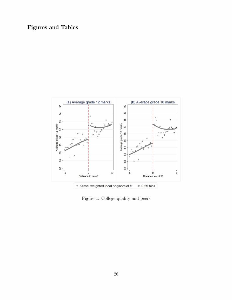
in lower quality colleges. This is shown in Table 1. The marginally admitted student is
surrounded by peers whose average score on the high school exit examination is 2.5 percentage
points higher than peers of a comparable student who just missed the cutoff. In Columns 2
and 3 we show that both male and female students in high-quality colleges are surrounded
by high-achieving peers. This systematic difference in peer ability is also evident when we
consider performance on another pre-treatment achievement test. Students in India also
write a similar high-stakes examination at the end of grade 10. An analysis of our sample’s
grade 10 scores in Table 1 also points towards the higher peer quality experienced by the
marginally admitted student. Figure 1 depicts the corresponding difference in peer quality.
Further, we show later in Section 4.3 that other factors such as teacher presence and student-
teacher ratios that could explain differences in college quality do not vary significantly around
the cutoff, indicating that variation in peer quality explains most of the variation in college
quality.
2.2 Sampling Strategy and Subject Recruitment
We constructed our sample in the following manner. First, to ensure representation of
colleges along the continuum of the college quality spectrum, we obtained the list of all
79 colleges affiliated with DU. Second, we drew a list of 58 colleges that offer courses in
commerce and/or economics streams. We focus on these two disciplines as they are among the
most popular and competitive disciplines and have significantly higher levels of enrollment
compared to other disciplines. The 58 colleges that offer courses in these two streams can be
7As cutoffs drop between admission rounds, it is possible for students to move ‘up’ to colleges where theynow become eligible. In the sample used for the analysis, we find that 26.5 percent of the students switchedcolleges during the admission process.
8While it is possible for students to seek transfers between colleges after the conclusion of the admissionprocess, it is not very common. In the empirical analysis, we exclude students who reported transferringbetween colleges at some point after the completion of the admission process.
5
further categorized into daytime coeducational colleges (31), daytime women-only colleges
(10), and evening coeducational colleges (17). Of the 31 daytime coeducational colleges, we
further exclude colleges that offer too few courses or use religious criteria or any criteria
other than high school exit examination scores for admissions, resulting in a list of 25 target
colleges. After considering admission cutoffs for each of these 25 colleges for three consecutive
years (2011-13), we identified 18 colleges that had consistently ranked admission cutoffs
across the three years for the two disciplines of economics and commerce, of which we could
implement our study in 15 colleges with varying cutoffs. We collected data on approximately
2000 second and third year students enrolled in these 15 colleges during January-March 2014
in regular class hours, in coordination with the teachers.
2.3 Data
In the first part of the study, we conducted incentivized experiments to obtain measures
of behavioral preferences.9 First, to capture subjects’ competitiveness and overconfidence
we used a simple number-addition task (similar to Niederle and Vesterlund, 2007). After a
practice session, participants had to predict their performance in advance, and also choose
between a piece-rate and tournament compensation scheme. Under the piece-rate scheme,
Rs. 10 was paid for every correct answer. Under the tournament scheme, Rs. 20 was paid
for every correct answer if the subject out-performed a randomly selected student of DU
who had solved the questions earlier.10 We define competitiveness as a dummy that takes a
value 1 if the subject chose the tournament compensation scheme and 0 if the subject chose
the piece-rate compensation scheme. We define overconfidence as the ratio of the predicted
performance to the student’s performance in the actual task.
Second, to measure risk preferences, we used the Gneezy and Potters (1997) investment
task. In this, subjects allocated a portion of their endowment (Rs. 150) to a risky lottery
and set aside the remainder. If they won the lottery based on a roll of a dice, the invested
amount was tripled and they also got any amount they set aside. Conversely, if they lost
the lottery, they only received the amount that was set aside. We define risk preference as
the proportion allocated to the risky lottery in the investment game.
In the second part of the study, we implemented a socioeconomic survey that collected details
9Subject instructions for the incentivized tasks are available from the authors upon request.10We implemented a pilot version of this game where 40 students from DU had participated, and their
performance is used for comparison in the tournament wage scheme.
6
on family background characteristics, school and college information, academic performance,
and participation in extra-curricular activities. To measure cognitive outcomes, we collected
data on scores on standardized university examinations. To measure personality traits, we
administered the 10-item Big Five inventory (Gosling et al., 2003) that consists of the fol-
lowing traits. Openness to experience, a tendency to be open to new aesthetic, cultural, or
intellectual experiences. Conscientiousness refers to a tendency to be organized, responsi-
ble, and hard working. Extraversion relates to an outward orientation of one’s interests and
energies oriented towards the outer world of people rather than the inner world of subjective
experience, characterized by sociability. Agreeableness is related to the tendency to act in
a cooperative and unselfish manner. Emotional stability (opposite of Neuroticism) is pre-
dictability and consistency in emotional reactions with absence of rapid mood changes.
Overall, we conducted 60 sessions with approximately 34 subjects per session. Each session
lasted about 75 minutes. No feedback was provided between or after the tasks. All subjects
received a show-up fee of Rs. 150. The average additional payment was Rs. 230. All subjects
participated only once in the study. To minimize wealth effects, additional payments were
based on one of the randomly chosen incentivized tasks.
3 Methodology
3.1 Empirical Specification
For estimating the returns to college quality, we first construct groupings of colleges based
on their relative selectivity. We use admission cutoffs, as exogenously announced by the
individual colleges, as the criteria to sort the 15 colleges in our sample into four ordered
categories such that, (i) colleges in a category have similar cutoffs, and (ii) colleges in the
higher categories have admission cutoffs that are consistently higher than the cutoffs of
colleges that belong to the lower categories. The 15 colleges in our sample are consequently
given four ranks ranging from 1 (highest rank) to 4 (lowest rank).
Next, for each rank we compute the minimum score required for admission into the group.
Cutoffs vary by student type where students differ in their current discipline (commerce and
economics), academic concentration in high school (science, commerce, and humanities),
gender, and year of entry. For example, a student seeking admission into economics, having
studied science in high school faces a different cutoff from a student who studied commerce
7
during high school. Further, some colleges also offer discounted cutoffs to female applicants.
Thus, for each rank of colleges we get a set of cutoffs that define the minimum score required
by each student type for admission into that college rank.
We are interested in estimating the returns to enrollment in a more selective college group
for which we construct three samples. In the first sample, colleges in rank 1 are assigned as
the treated group (high-quality college) and the remaining colleges (in ranks 2, 3 and 4) are
assigned as lower-quality colleges. Thus, in the first sample a student is considered to be
in the treated group if she is enrolled in any of the colleges in rank 1. In the next sample,
colleges in ranks 1 and 2 are assigned to the treated group and the remaining colleges (ranks
3 and 4) are assigned to the low-quality college group. Finally, a third sample is constructed
where colleges ranked 1, 2, and 3 are assigned to the high-quality college group and colleges
in rank 4 are in the low-quality college group. Following Abdulkadiroglu et al. (2014) and
Pop-Eleches and Urquiola (2013), we construct our final analysis sample by ‘stacking’ the
three samples together, and estimate a single average treatment effect measuring the impact
of enrollment in a high-quality college.
Of course, enrollment in the high-quality college is endogenous as not all students who are
eligible to enroll in a higher quality college do so.11 To account for this, we use a “fuzzy”
regression discontinuity (RD) design where enrollment is instrumented by eligibility to enroll
in a more selective college (Hahn et al., 2001; Lee and Lemieux, 2010). In particular, we
estimate the following set of instrumental variable regressions where the first-stage regression
is:
TRij = α0 + α1Tij + α2dij + α3d2ij + α4dijTij + α5d
2ijTij +
K∑l=6
αlXlij + ηj + εij (1)
and the corresponding second-stage regression is:
Yij = δ0 + δ1TRij + δ2dij + δ3d2ij + δ4dijTRij + δ5d
2ijTRij +
K∑l=6
δlXlij + ηj + µij (2)
11Similarly, we also have a few instances where students who are ineligible for a higher ranked college areadmitted to that college. Overall, in the stacked sample used in the analysis, only 0.35 percent of the subjectswho have a negative distance from the cutoff are enrolled in a higher ranked college and approximately 6percent of the subjects who have a positive distance from the cutoff are enrolled in a lower ranked college.
8
where Yij in equation (2) is the outcome variable of interest for student i of type j. Equation
(1) is a linear probability model where TRij takes the value 1 if student i of type j is treated,
i.e., enrolled in a high-quality college. The running variable, dij, is computed as the difference
between student i′s high school exit examination score and the relevant college rank-specific
cutoff faced by her type j. The instrument is a dummy variable for eligibility, Tij, that takes
a value 1 if dij is non-negative, 0 otherwise. We allow for non-linearity in the relationship
between the outcomes and the running variable by including a quadratic specification in the
running variable as well as allow the estimated returns to college quality to vary on each side
of the cutoff by allowing interactions between the TR dummy and di and d2i . Our regressions
also include cutoff fixed effects (ηj) where the cutoffs vary by student types. This allows us
to obtain the relevant counterfactual for a student enrolled in the high-quality college - a
student of the same type (i.e., currently enrolled in the same discipline, with the same high
school academic concentration, same gender, and same year of admission) who marginally
missed the relevant cutoff. We also include a vector of predetermined characteristics (Xs)
such as mother’s education, father’s education, private school enrollment, age, family income,
and religion in the regressions to improve the precision of our estimates. Finally, µij and εij
are iid error terms.
The coefficient estimate on TR in equation (2) gives us the local average treatment effect
(LATE) of being enrolled in a selective college group. Since the running variable is discrete,
following Lee and Card (2008), we cluster our standard errors with respect to 0.25 bins
of the running variable. The choice of the bandwidth is another important issue in RD
analysis. Since we have various outcome variables, we fix the bandwidth to be 5 percentage
points around the cutoff for the main analysis. Nonetheless, in Section 4.4, we show that our
results are robust to using outcome-specific optimal bandwidths determined by the procedure
outlined in Calonico et al. (2014).
For the analysis, we exclude all those students whose admissions were not based on their
high school exam scores. This includes students belonging to historically disadvantaged
backgrounds (Scheduled Castes, Scheduled Tribes, and Other Backward Classes) for whom
affirmative action policies mandate a fixed number of seats; students admitted on the basis of
excellence in sports or other extra-curricular activities; those who transferred from one college
to another after enrollment or switched disciplines within a college; and those providing
insufficient identification information. From an initial sample of 2065, 1331 subjects remain
after making exclusions as discussed above.12 After stacking our data and limiting to a
12In our initial sample, 29 percent are affirmative action beneficiaries, 4.8 percent got admitted based
9
bandwidth of five percentage points around the cutoff, the analysis sample is 2395. Finally,
as the literature on educational interventions, and more specifically on the effects of school
and college quality documents significant heterogeneity by gender (e.g., Kling et al., 2005;
Hastings et al., 2006; Jackson, 2010), we also report our results for samples of males and
females separately.
As we wish to estimate the effects of admission into a higher quality college versus the
counterfactual of a lower quality college, the ideal sample would comprise students who
strictly prefer higher quality colleges to the lower quality ones such that a score above the
cutoff would lead to admission in a higher quality college, and scoring below the relevant
cutoff would result in admission in a lower quality college. The student allocation mechanism
used in DU is different from the more commonly observed centralized mechanisms such as
the Boston school choice mechanism (Abdulkadiroglu et al., 2014), the student or college
proposing deferred acceptance mechanisms, or the top trading cycle mechanism. In DU,
students are admitted through a decentralized admission process wherein they apply to
college-disciplines individually and do not have to submit a preference ranking over disciplines
and/or colleges to any central authority. Therefore, this decentralized allocation process does
not provide the underlying preferences of the applicants and all we observe is the current
college that the student is enrolled in, along with her high school exit examination score, and
the cutoffs she faced at the time of admission. Nonetheless, note that with a fixed supply
of seats, the higher cutoffs at colleges are a reflection of (greater) excess demand for those
seats. It is then reasonable to assume that the average student prefers admission into a
college with higher cutoffs as opposed to one with lower cutoffs.
3.2 Testing Validity of the RD Design
The RD model relies on two assumptions: (a) there is no manipulation of the assignment
variable at the cutoff, and (b) the probability of being enrolled in a better-quality college is
discontinuous at the cutoff. This is also proof of a strong first-stage regression, necessary for
obtaining a valid second stage estimate.
The estimation strategy would result in biased estimates if students could perfectly control
the side of the cutoff they will fall on. However, this is not possible under the admission
process in DU. First, high school exit examinations follow a double blind grading procedure,
on sports and other activities, 0.3 percent migrated within or across colleges, and 0.6 percent providedinsufficient information.
10
making manipulation difficult, if not outright impossible. Second, at the time of application
to DU colleges, students are not aware of the precise cutoffs that will determine admissions
that year.13 Moreover, since the rule for determining these cutoffs is never public knowl-
edge, students cannot perfectly predict future cutoffs. Overall, it is virtually impossible
for students to perfectly manipulate the side of the college cutoff they will ultimately fall
on.14
As colleges are required to simultaneously reduce cutoffs till there are no vacancies, it is
very unlikely that students just above the cutoff differ systematically from those just below
the cutoff on unobservables. We can, however, formally check for discontinuities in other
predetermined characteristics such as mother’s education, father’s education, private high
school enrollment, age, family income, and religion by estimating the following reduced form
regression:
Xij = β0 + β1Tij + β2dij + β3d2ij + β4dijTij + β5d
2ijTij + ηj + υij (3)
Where X is the vector of predetermined background characteristics and the right hand side
variables are as defined in equations (1) and (2) above. The results from these regressions
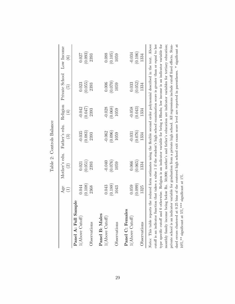
are presented in Table 2. We find that the impact of the treatment indicator, that is, being
eligible to enroll in a higher quality college on the predetermined variables is mostly small
and never significantly different from zero, confirming the validity of the RD design for
the pooled sample (Panel A), males (Panel B), and females (Panel C). The corresponding
graphical representations are provided in Figures A1 - A3 in the online Appendix.
Next, we check if the probability of enrollment is indeed discontinuous at the cutoff. In Figure
2, we plot the proportion of students enrolled in a high-quality college in each 0.25 bin against
the distance from the cutoff. This is done for the pooled sample and separately for males
and females as well. In all three sub-figures, we see a clear discontinuity in the probability of
enrolling in a more selective college at the cutoff, indicating the appropriateness of the RD
design. A formal estimation of the first-stage relationship between enrollment in a selective
13Based on historical trends, students may have an estimate of the range of the cutoff, but this does notinvalidate our analysis since perfect manipulation is impossible.
14The RD literature uses the presence of bunching just above the threshold as an indicator of manipula-tion (typically tested using the McCrary test). However, the college admission process followed in DU byconstruction results in bunching of students just above the threshold and hence is not useful for detectingmanipulation in the sample.
11
college and eligibility is provided in Table 3. We find that on average, students who are
eligible to enroll in a selective college are 68 percent more likely to do so, indicating a strong
revealed preference for more selective colleges. We find similar strong effects of the eligibility
to enroll in a selective college for both males and females. As compliance with DU admission
rules is not perfect, we use a fuzzy RD design and in the sections that follow, present results
from the corresponding IV specification discussed in equations (1) and (2).
4 Results
4.1 Summary Statistics
In Table 4, we present descriptive statistics for our sample. In Panel A, we summarize
average performance on standardized university-level examinations, our measure of academic
attainment during college.15 The average score is 70 percent with no significant gender
differences.
In Panel B, we summarize average choices of the elicited behavioral preferences: compet-
itiveness, overconfidence, and risk. In our sample, 31 percent of the subjects are deemed
as being competitive as they choose the tournament payment scheme. The average student
is overconfident as the ratio of the expected number of correct answers to the number cor-
rectly solved in the actual task is 1.6, significantly higher than 1. These findings are in line
with other papers in the literature that find that about one-third of subjects choose the
tournament wage scheme and that subjects often irrationally overestimate their own abili-
ties across tasks (e.g., Niederle and Vesterlund, 2007; Dasgupta et al., 2015). Finally, the
average investment of 47 percent in the risky asset, our measure of risk preference, is in the
range of 44.67-70.86 percent for student populations as reported in Charness and Viceisza
(2016). It is not surprising that there are significant gender differences with males being
more competitive and less risk averse than females (see Niederle, 2016 for a review).
In Panel C, we summarize subjects’ Big Five personality traits: openness to experience, con-
scientiousness, extraversion, agreeableness, and emotional stability. In our sample, subjects
report a higher score on agreeableness, conscientiousness, and openness to experience than
they do for extraversion and emotional stability. There are significant differences by gender
15The university follows a semester system where an academic year consists of 2 semesters, with examsheld in December and May. Since our study was conducted during January-March, for second and thirdyear students, we have the average exam scores based on 3 semesters and 5 semesters respectively.
12
with females being more extrovert, conscientious and agreeable, and less emotionally stable
than males (p− value ≤ 0.01 in all cases except extraversion). Similar gender differences in
personality traits are also noted across several cultural contexts (Schmitt et al., 2008).
Finally, in Panel D, we present descriptive statistics on background characteristics. The
average age of the students is close to 20, with little variation. Over 90 percent of the
students are Hindus (the dominant religion in India), 85 percent attended a private high
school, and 73-79 percent of students have either a highly educated mother or father (college
degree or higher). A third of the sample comes from low-income households (i.e. those
earning less than Rs. 50,000 per month).16
4.2 Returns to College Quality: Cognitive, Behavioral, and Per-
sonality
In Table 5, we present the impacts of enrollment in a more selective college on cognitive (in
Panel A), behavioral (in Panel B), and personality outcomes (in Panel C) for the pooled sam-
ple, males, and females in Columns 1, 2, and 3 respectively. These are IV estimates obtained
from equation (2). While curriculum and examinations are the same within a discipline
across colleges of DU, marginal admission into a more selective college exposes students to
high-achieving peers. Looking at the impact estimates on the standardized university-level
examination scores for the pooled sample in Column 1 of Panel A, we find that compared
to students in lower quality colleges, marginally admitted students in higher quality colleges
experience a 1.1 percentage point increase in their average university examination scores.
Upon further examining these effects by gender, it is apparent that this overall impact is
entirely driven by the significant effects on females’ test scores with no effect for males
(Columns 2 and 3). In particular, females, on average, score 2.6 percentage points higher on
the university examinations relative to females in lower quality colleges, translating into an
approximate increase of 3.8 percent over the control group’s mean of 69 percent. Our find-
ing that females make significant academic gains from exposure to peer environments with
little or no accompanying effects on males has also been found in other studies of school
and college quality (e.g., Jackson, 2010; Hastings et al., 2006) as well as other educational
interventions (e.g., Angrist et al., 2009; Angrist and Lavy, 2009). Further, we show later in
Section 4.3 that females enrolled in more selective colleges are almost 31 percentage points
16According to the nationally representative India Human Development Survey of 2011-12, the averageyearly income for upper caste households is approximately Rs. 180,000, indicating that our analysis samplefares significantly better than the average.
13
more likely to have higher attendance rates than their counterparts in less selective colleges.
On the other hand, we find no such effect of college quality on male attendance rates. This
gender difference in attendance rate is likely to explain the observed gender gap in academic
returns to better college and peer environments.
We also estimate the returns to enrollment in a selective college on three measures of be-
havior: competitiveness, overconfidence, and risk. The results are reported in Panel B of
Table 5. Pooled results indicate that the marginally admitted student experiences a decline
in overconfidence with no significant effects on competitiveness and risk preferences. On
disaggregating the sample by gender, we find no significant effects on males. We observe
overconfidence among marginally admitted females to reduce by 0.70 units or, approximately
42 percent of the control mean. We also find that females enrolled in more selective colleges
invest almost 13 percentage points more in the investment game, thereby being less risk
averse than their female counterparts who just miss out on a more selective college. This
effect is substantial given that the control mean is 43.3 percent. To the extent that females
are more risk averse than males, and this gender gap in risk preferences has implications
for occupational choice and other economic decision-making, this result suggests that higher
quality colleges may result in a narrowing of this gender gap. The observed decline in risk
aversion and overconfidence points towards an increase in rationality among marginally ad-
mitted females. Specifically, as per the expected utility theory framework, given the nature
of the investment game used to elicit risk preferences as described in Section 2.3, a risk-
neutral individual should invest the full amount in the risky lottery. Therefore, an increase
in the proportion invested in the risky lottery by females in selective colleges suggests that
exposure to, and learning from, higher ability peer groups leads them to assess the risk in
a more rational manner. Similarly, for the marginal student, being surrounded by smart
peers, allows her to update her beliefs about her (relative) ability, leading to a decline in
overconfidence. Since overconfidence is positively and risk aversion is negatively related to
competitiveness, a decline in risk aversion and overconfidence could plausibly explain why
we do not observe any significant effects of college quality on competitiveness.
The last set of impact estimates pertains to personality: Big Five traits of openness to ex-
perience, conscientiousness, extraversion, agreeableness, and emotional stability (see Panel
C, Table 5). In the pooled sample, we find that enrollment in a more selective college neg-
atively affects extraversion by 0.27 standard deviations with no effect on other traits. We
find substantial gender differences in the impact on personality: extraversion and conscien-
tiousness among marginally admitted males reduces by 0.48 standard deviations and 0.55
14
standard deviations, respectively. Taken together, these estimates for male students suggest
a diminished self-concept stemming from their lower academic position within their college
rank, resulting in negative effects on economically valuable personality traits. Murphy and
Weinhardt (2016) also find males to be influenced more significantly on account of rank
concerns. Using alternative measures as proxies for these personality traits reinforces our
findings. In results reported in Table A1 in the online Appendix, membership in college-
level societies, another measure of extrovert behavior, is also lower among males enrolled
in higher quality colleges. Similarly, we also find that males at the margin of admission in
higher quality colleges report lower grit, which is highly correlated with conscientiousness.17
We also observe a decline in openness to experience and agreeableness for males, though
neither is statistically significant. In light of recent findings that show that conscientiousness
and extraversion matter for academic performance (Lundberg, 2013), the adverse effects on
these personality traits for marginally admitted males might explain why we observe no gains
in test scores from exposure to a better college environment.
4.3 Pathways
Owing to the design of the admissions process in colleges at DU, we have so far shown and
argued that differences in peer quality is the likely channel driving our main results, as it
varies significantly across colleges. In this section, we explore a variety of other potential
channels that could explain our main findings.
In Column 1 in Table 6, we examine differences in attendance rates. We construct a binary
variable for high attendance that takes a value 1 if subjects report having class attendance
rates of 75 percent and higher, and 0 if attendance is below 75 percent. We find that while
there is no significant difference for males in the probability of high attendance, females
enrolled in selective colleges have a greater probability of high attendance than females in less
selective colleges. This indicates that they are present in class more often and therefore have
an opportunity to learn from and engage with their peers, making it one of the competing
explanations for gains on cognitive and behavioral outcomes. This finding fits in with the
general observed pattern of females having better study habits (Angrist et al., 2009; Angrist
and Lavy, 2009; Hastings et al., 2006).
Next, we examine relative attendance by asking subjects to indicate attendance relative
17Grit is the tendency to sustain interest in and effort towards very long-term goals (Duckworth andQuinn, 2009).
15
to their classmates. In Column 2, we construct an outcome variable that takes the value
1 if the subject attended classes less often than her classmates. We find that marginally
admitted males are more likely to skip classes than their classmates. This points towards
weakened self-concept among males on account of their lower academic position in their
college rank, potentially indicating higher mental or psychic costs of investing effort. Elsner
and Isphording (2016a) also find a similar effect in that students with lower ordinal rank are
more likely to be absent from classes.
Subjects could also experience learning gains due to complementary investments in education
undertaken by parents and students in the form of external tutorials and remedial classes.18
These can improve test scores independent of the college and peer environment. However,
as shown in Column 3 of Table 6, we do not find a discontinuity in the probability of using
external tutorials for either males or females.
Finally, differences in indicators of teacher quality and presence could also matter for stu-
dents’ academic and non-academic outcomes (e.g., Hoffmann and Oreopoulos, 2009; Chetty
et al., 2014; Jackson, 2012). It should be noted that teacher salaries are the same across col-
leges in DU. As a measure of teacher quality and presence, we asked students if classes were
cancelled frequently by teachers. Results in Column 4 show no discontinuity in the proba-
bility of classes being cancelled. Finally, results in Column 5 indicate that student-teacher
ratio, an additional measure of college quality, also does not vary around the cutoff.
4.4 Robustness
We show here that the LATE estimates reported earlier in Table 5 are robust to several
econometric concerns such as: inclusion of controls, choice of the polynomial order, band-
width selection, and estimation technique. These results are presented for the pooled sample,
males, and females in Panels A, B and C respectively of Tables 7 and 8 .
First, while our main estimates control for several predetermined background characteristics
to improve precision, we now show that the results remain robust to excluding these controls.
Second, to check for specification bias arising from the choice of second-order polynomial
function, we present the impact of enrolling in a selective college on all outcomes using a
flexible cubic polynomial function and find that the results are mostly similar to the ones
presented earlier in Table 5. Third, while we have used rectangular weights in the main
18Another parental response could be spending time with children to help them with academic materialsand homework as in Pop-Eleches and Urquiola (2013). However, that is unlikely at college level.
16
analysis, we find that using triangular weights that assign greater weights to observations
closer to the cutoff does not qualitatively alter the results. Fourth, while we have used a
common bandwidth of 5 percentage points for all the outcomes in Table 5, we now restrict
our data to the optimal bandwidth prescribed by Calonico et al. (2014) separately for each
outcome variable, and find our results to be robust to the width of the window around the
cutoff. Finally, our results remain robust to clustering at the level of the student or the
session.19
As discussed in Section 3.1, in estimating the effect of admission into a higher quality college
versus a lower quality college, we implicitly assume that students prefer a higher quality
college to a lower quality one. We now show that our results are largely robust to relaxing
this assumption. In the survey, we asked students to rank a subset of the surveyed colleges
across our four ranks. While we did ask students to rank the colleges as they would have at
the time of admission, this ranking is bound to be subject to measurement error. Nonetheless,
we use this information in the following way to assess the robustness of our results. While
constructing each of our RD samples, as discussed in Section 3.1, we limit our sample to
students who strictly rank all the treated colleges higher than the lower-quality colleges and
do not rank any of the low-quality colleges at least as high as any of the treated colleges.
While the sample now is limited, we find that the effects on most behavioral and personality
traits continue to hold (Table A2 in the online Appendix).
4.5 Heterogeneity
In this section, we explore if the effects of college quality vary by, (i) family background
characteristics, and (ii) the degree of college selectivity.
Current research indicates that growing up in households characterized by low socioeconomic
status can adversely affect the formation and development of behavior and personality traits
because of lower parental investment in terms of time and money (e.g., Deckers et al.,
2016; Fletcher and Wolfe, 2016). If this is indeed the case, then can higher quality college
environments have compensatory effects on the development of these socioemotional skills?
On the other hand, there may be dynamic complementarities as proposed by Cunha and
Heckman (2007) such that students from well-off backgrounds may be equipped with a better
stock of skills owing to early investments that allow them to gain more from their college
environments. We examine the interactive effects of family background characteristics with
19These results are available from the authors upon request.
17
college quality to allow for the returns to enrolling in a selective college to vary by family
income and parental education. The results are reported in Table 9. Given the gender-
differentiated returns to college quality noted so far, we report the heterogeneity results
for males and females separately. The coefficients of interest are the interaction terms of
the indicator of enrollment in a more selective college with the indicator of low income/low
parental education.20
Panels A and B of Table 9 report the heterogeneous effects of low income and low parental
education for males respectively while Panels C and D report the results for females. The first
column indicates that there is no heterogeneity in the cognitive returns to college quality by
family background. Columns 2-4 report the results for behavioral preferences: competitive-
ness, overconfidence, and risk. Column 4 shows that females from low-income households
enrolled in more selective colleges invest 5.6 percentage points more compared to females
from high-income households that are enrolled in a selective college. Similarly, among those
enrolled in more selective colleges, females with less educated parents invest significantly
more than those whose parents are highly educated. As high socioeconomic status is usu-
ally correlated with less risk averse behavior (e.g., Dohmen et al., 2011), more selective
colleges mitigate the gap in risk preferences between students from varying socioeconomic
backgrounds. Finally, on examining the socioemotional traits in Columns 5-9, we find that
females from low-income households enrolled in more selective colleges report higher scores
on agreeableness than those from high-income households, implying some gains in their abil-
ity to engage in interpersonal interactions. However, we do not find a corresponding effect
when examining heterogeneity by parental education. Finally, the remaining columns indi-
cate that we do not find any differential effects on other Big Five traits of being in selective
colleges based on socioeconomic status.
We proceed to explore if the effects vary by the selectivity of the college. The existing litera-
ture has mainly studied effects of enrollment in top educational institutions (e.g., Hoekstra,
2009; Abdulkadiroglu et al., 2014) or average effects of enrolling in relatively more selec-
tive institutions using data from a range of institutions (e.g., Jackson, 2010; Lucas and
Mbiti, 2014). However, returns to school and educational quality may be non-linear and
vary across the quality distribution. For example, Hoekstra et al. (2016) examine schools of
varying selectivity within the same educational context in China and find effects stemming
20In terms of the IV regressions discussed in Section 3, we add the interaction of the indicator of enrollmentin a selective college and the indicator of socioeconomic status as an additional endogenous regressor andadd the interaction of the indicator of eligibility for enrollment in a selective college and the indicator ofsocioeconomic status as an additional instrument.
18
from enrollment in only the most elite schools. In a similar vein, in our setting, we examine
if behavioral responses to college and peer environments differ depending on how selective
the college is. For this purpose, we re-estimate our regressions separately examining (i) the
effect of enrolling in a rank 1 (most selective) colleges in Panels A and B of Table 10, and
(ii) the effects of college quality excluding rank 1 college cutoffs in Panels C and D of Table
10. The returns to college quality may vary across these two samples as the scope for im-
provement based on learning from peers may be lower in rank 1 colleges. Furthermore, the
adverse effects of lower relative rank on academic self-concept may be more acutely felt in
the more selective colleges. We find that enrolling in a rank 1 college reduces conscientious-
ness, openness to experience, and overconfidence among marginally admitted males, and
an increase in risk taking and reduction in overconfidence for females. In contrast, we find
that excluding rank 1 college cutoffs reduces extraversion for males and increases risk taking
among females. Overall, the results suggest that males are more likely to be susceptible
to relative rank concerns in the most selective colleges which results in negative effects on
personality and behavior reported in Panel A compared to Panel C, Table 10. On the other
hand, for females, the results in Panel B and Panel D remain largely similar.
5 Conclusion
The existing empirical work on the returns to college quality has largely focused on test scores
as outcomes of human capital with resulting mixed evidence. Scant attention has been paid
to non-cognitive and socioemotional traits, facets of human capital that recent research has
documented as being tremendously important for one’s economic progress.
In this paper, our aim has been to fill this critical gap by examining the effects of college
selectivity on cognitive, behavioral, and socioemotional outcomes, using novel data collected
from a large sample of students at a leading Indian university. Exploiting the variation in
college admission cutoffs, we compare students just above the cutoff with those just below
the cutoff to determine the causal impact of enrollment in a selective college, where they
are exposed to relatively high-achieving peers. We find that a marginally admitted student
in a more selective college experiences an improvement in scores on standardized university
exams, and this effect is driven by females. In terms of behavioral and personality traits,
we find that females just above the cutoff become less risk averse and less overconfident,
indicating an increase in rationality. On the other hand, males in these colleges experience
declines in extraversion and conscientiousness pointing towards a weakened self-concept due
19
to a lower relative rank in their peer group. Further, we are also able to show that variation
in college quality stems mainly from variation in peer quality with no differences in teacher
presence or student-teacher ratios around the cutoff.
Some caveats remain. First, it should be noted that our study does not encompass the entire
population of University of Delhi students. Also, since this is one of the premier universities
in India, its students are not representative of the average Indian college student. Second,
while at this point the study is unable to comment on observable labor market outcomes of
this cohort of students, in future work, we aim to do so.
20
References
Abdulkadiroglu, A., Angrist, J.D., and Pathak, P.A. (2014). The Elite Illusion: Achievement
Effects at Boston and New York Exam Schools. Econometrica, 82(1), 137-196.
Ajayi, K.F. (2014). Does School Quality Improve Student Performance? New Evidence from
Ghana. Working Paper.
Almas, I., Cappelen, A.W., Salvanes, K.G., Sorensen, E.O., and Tungodden, B. (2016).
What explains the gender gap in college track dropout? Experimental and administrative
evidence. American Economic Review: Papers & Proceedings, 106(5), 296-302.
Almlund, M., Duckworth, A.L., Heckman, J.J. and Kautz, T. (2011). Personality psychology
and economics, in E.A. Hanushek, S. Machin and L. Woessmann, (eds.), Handbook of the
Economics of Education, vol. 4, pp. 1-181, Amsterdam: North-Holland.
Angrist, J., Lang, D., and Oreopoulos, P. (2009). Incentives and Services for College Achieve-
ment: Evidence from a Randomized Trial. American Economic Journal: Applied Economics,
1(1), 136-63.
Angrist, J., and Lavy, V. (2009). The Effects of High Stakes High School Achievement
Awards: Evidence from a Randomized Trial. American Economic Review, 99(4), 301-
331.
Borghans, L., Duckworth, A.L., Heckman, J.J., and ter Weel, B. (2008). The Economics
and Psychology of Personality Traits. Journal of Human Resources, 43(4), 972-1059.
Calonico, S., Cattaneo, M. D., and Titiunik, R. (2014). Robust Nonparametric Confidence
Intervals for Regression-Discontinuity Designs. Econometrica, 82(6), 2295-2326.
Camerer, C. F. and D. Lovallo (1999). Overconfidence and Excess Entry: An Experimental
Approach. American Economic Review, 89, 306-318.
Castillo, M., Petrie, R. and Torero, M. (2010). On the Preferences of Principals and Agents.
Economic Inquiry, 48(2), 266-273.
Charness, G., and Viceisza, A. (2016). Three risk elicitation methods in the field: evidence
from rural Senegal. Review of Behavioral Economics, 3(2), 145-171.
Chetty, R., Friedman, J.N., Rockoff, J.E. (2014). Measuring the Impacts of Teachers II:
Teacher Value-Added and Student Outcomes in Adulthood. American Economic Review,
104(9), 2633-79.
21
Chuang, Y., and Schechter, L. (2015). Stability of experimental and survey measures of
risk, time, and social preferences: A review and some new results. Journal of Development
Economics, 117, 151-170.
Cicala, S., Fryer, R. G., and Spenkuch, J. L. (2016). Comparative Advantage in Social
Interactions. Working paper.
Cunha, F., and Heckman, J.J. (2007). The technology of skill formation. American Eco-
nomic Review Papers & Proceedings, 97(2), 31-47.
Dasgupta, U., Gangadharan, L., Maitra, P., Mani, S., and Subramanian, S. (2015). Choosing
to be Trained: Do Behavioral Traits Matter? Journal of Economic Behavior & Organization,
110, 145-159.
Deckers, T., Falk, A., Kosse, F., and Schildberg-Horisch, H. (2015). How Does Socio-
Economic Status Shape a Childs Personality? IZA Working Paper No. 8977.
Dohmen, T., Falk, A., Huffman, D., Sunde, U., Schupp, J., and Wagner, G. G. (2011).
Individual risk attitudes: Measurement, determinants and behavioral consequences. Journal
of the European Economic Association, 9(3), 522-550.
Duckworth, A.L, and Quinn, P.D. (2009). Development and validation of the Short Grit
Scale (Grit-S). Journal of Personality Assessment, 91, 166-174.
Elsner, B., and Isphording, I. (2016a). A Big fish in a small pond: Ability rank and human
capital investment. Journal of Labor Economics, forthcoming.
Elsner, B., and Isphording, I. (2016b). Rank, sex, drugs, and crime. Journal of Human
Resources, forthcoming.
Epple, D., and Romano, R. (2011). Peer effects in education: A survey of the theory and
evidence. In J. Benhabib, A. Basin and M. Jackson (Eds.) Handbook of Social Economics,
1053-1163.
Feld, J., and Zolitz, U. (2017). Understanding peer effects: on the nature, estimation, and
channels of peer effects. Journal of Labor Economics, forthcoming.
Fletcher, J. M., and Wolfe, B. (2016). The importance of family income in the formation
and evolution of non-cognitive skills in childhood. Economics of Education Review, 54,
143-154.
Flory, J. A., Leibbrandt, A., and List, J. A. (2015). Do competitive work places deter female
22

workers? A large-scale natural field experiment on job entry decisions. Review of Economic
Studies, 82(1), 122-155.
Gneezy, U. and Potters, J. (1997). An experiment on risk taking and evaluation periods.
Quarterly Journal of Economics, 112(2), 631-645.
Gosling, S.D., Rentfrow, P.J., and Swann Jr., W.B. (2003). A very brief measure of the
Big-Five personality domains. Journal of Research in Personality, 37, 504-528.
Hahn, J., Todd, P., and Van der Klaauw, W. (2001). Identification and estimation of
treatment effects with a regression-discontinuity design. Econometrica, 69(1), 201-209.
Hanushek, E.A., and Woessmann, L. (2008). The role of cognitive skills in economic devel-
opment. Journal of Economic Literature, 46(3), 607-668.
Hastings, J.S., Kane, T., and Staiger, D. (2006). Gender, performance and preferences:
do girls and boys respond differently to school environment? Evidence from school as-
signment by randomized lottery. American Economic Review Papers & Proceedings, 96(2),
232-236.
Heckman, J.J., Stixrud, J., and Urzua, S. (2006). The effects of cognitive and non-cognitive
abilities on labor market outcomes and social behavior. Journal of Labor Economics, 24(3),
411-482.
Hoekstra, M. (2009). The effect of attending the flagship state university on earnings: a
discontinuity-based approach. Review of Economics and Statistics, 91(4), 717-724.
Hoekstra, M., Mouganie, P., and Wang, Y. (2016). Peer quality and the academic benefits
to attending better schools. Working Paper.
Hoffmann, F., and Oreopoulos, P. (2009). Professor qualities and student achievement.
Review of Economics and Statistics, 91(1), 83-92.
Jain, T., and Kapoor, M. (2015). The impact of study groups and roommates on academic
performance. Review of Economics and Statistics, 97(1), 44-54.
Jackson, C. K. (2010). Do Students Benefit from Attending Better Schools? Evidence from
Rule-based Student Assignments in Trinidad and Tobago. Economic Journal, 120(549),
1399-1429.
Jackson, C. K. (2012). Non-Cognitive Ability, Test Scores, and Teacher Quality: Evidence
from 9th Grade Teachers in North Carolina. NBER Working Paper No. 18624.
23
Kaufmann, K.M., Messner, M., and Solis, A. (2015). Elite higher education, the marriage
market, and intergenerational human capital. Working Paper.
Kling, J.R., Ludwig, J., and Katz, L.F. (2005). Neighborhood effects on crime for female and
male youth: evidence from a randomized housing mobility experiment. Quarterly Journal
of Economics, 120(1), 87-130.
Koellinger, P., Minniti, M., and Schade, C. (2007). ‘I think I can, I think I can’: Overconfi-
dence and Entrepreneurial Behavior. Journal of Economic Psychology, 28, 502 - 527.
Lee, D.S., and Card, D. (2008). Regression discontinuity inference with specification error.
Journal of Econometrics, 142, 655-674.
Lee, D. S., and Lemieux, T. (2010). Regression Discontinuity Designs in Economics. Journal
of Economic Literature, 48(2), 281-355.
Lucas, A.M., and Mbiti, I.M. (2014). Effects of School Quality on Student Achievement:
Discontinuity Evidence from Kenya. American Economic Journal: Applied Economics, 6(3),
234-263.
Lundberg, S. (2013). The College Type: Personality and Educational Inequality. Journal of
Labor Economics, 31(3), 421-441.
Malmendier, U., and Tate, G. (2005). CEO overconfidence and corporate investment. Jour-
nal of Finance, 60(6), 2661-2700.
Marsh, H., Seaton, M., Trautwein, U., Ludtke, O., Hau, O’Mara, A., and Craven, R. (2008).
The Big Fish Little Pond Effect Stands Up to Critical Scrutiny: Implications for Theory,
Methodology, and Future Research. Educational Psychology Review, 20(3), 319-350.
Murphy, R., and Weinhardt, F. (2016). Top of the class: The importance of ordinal rank.
Working Paper.
Niederle, M. (2016). Gender. In J.H. Kagel and A.E. Roth (Eds.) Handbook of Experimental
Economics, Vol. 2, 481-553.
Niederle, M. and Vesterlund, L. (2007). Do Women Shy Away from Competition? Do Men
Compete to Much? Quarterly Journal of Economics, 122(3), 1067-1101.
Oreopoulos, P., and Salvanes, K.G. (2011). Priceless: The nonpecuniary benefits of school-
ing. Journal of Economic Perspectives, 25(1), 159-184.
24
Pop-Eleches, C., and Urquiola, M. (2013). Going to a Better School: Effects and Behavioral
Responses. American Economic Review, 103(4), 1289-1324.
Rubinstein, Y., and Sekhri, S. (2013). Public Private College Educational Gap in Developing
Countries: Evidence on Value Added versus Sorting from General Education Sector in India.
Working paper.
Saavedra, J. (2009). The learning and early labor market effects of college quality: a regres-
sion discontinuity analysis. Working paper.
Sacerdote, B. (2011). Peer Effects in Education: How Might They Work, How Big Are They
and How Much Do We Know Thus Far? Handbook of the Economics of Education, Vol. 3,
249-277.
Schmitt, D. P., Realo, A., Voracek, M., and Allik, J. (2008). Why can’t a man be more
like a woman? Sex differences in Big Five personality traits across 55 cultures. Journal of
Personality and Social Psychology, 94, 168-182.
Schurer, S., Kassenboehmer, S.C., and Leung, F. (2015). Do universities shape their students
personality? IZA DP No. 8873.
Specht, J., Egloff, B., and Schmukle, S.C. (2011). Stability and change of personality across
the life course: the impact of age and major life events on mean-level and rank-order stability
of the Big Five. Journal of Personality and Social Psychology, 101(4), 862-882.
25
Figures and Tables
Figure 1: College quality and peers
26
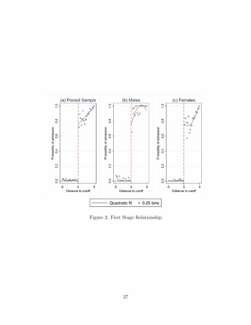
Figure 2: First Stage Relationship
27
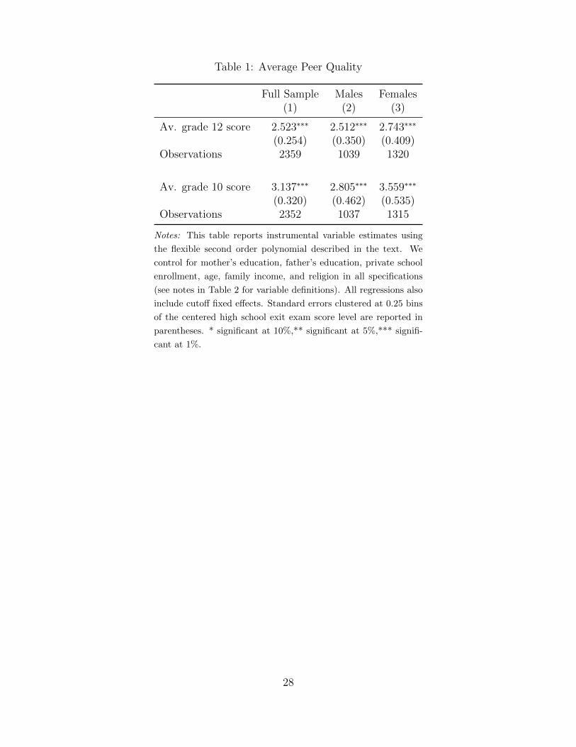
Table 1: Average Peer Quality
Full Sample Males Females(1) (2) (3)
Av. grade 12 score 2.523∗∗∗ 2.512∗∗∗ 2.743∗∗∗
(0.254) (0.350) (0.409)Observations 2359 1039 1320
Av. grade 10 score 3.137∗∗∗ 2.805∗∗∗ 3.559∗∗∗
(0.320) (0.462) (0.535)Observations 2352 1037 1315
Notes: This table reports instrumental variable estimates using
the flexible second order polynomial described in the text. We
control for mother’s education, father’s education, private school
enrollment, age, family income, and religion in all specifications
(see notes in Table 2 for variable definitions). All regressions also
include cutoff fixed effects. Standard errors clustered at 0.25 bins
of the centered high school exit exam score level are reported in
parentheses. * significant at 10%,** significant at 5%,*** signifi-
cant at 1%.
28
Tab
le2:
Con
trol
sB
alan
ce
Age
Mot
her
’sed
u.
Fat
her
’sed
u.
Rel
igio
nP
riva
teS
chool
Low
Inco
me
(1)
(2)
(3)
(4)
(5)
(6)
Pan
el
A:
Fu
llS
am
ple
1(A
bov
eC
uto
ff)
0.04
40.
021
-0.0
35-0
.042
0.02
30.
027
(0.1
08)
(0.0
51)
(0.0
83)
(0.0
47)
(0.0
55)
(0.0
93)
Ob
serv
atio
ns
2368
2393
2393
2393
2393
2393
Pan
el
B:
Male
s1(
Ab
ove
Cu
toff
)0.
043
-0.0
40-0
.062
-0.0
280.
006
0.08
8(0
.188
)(0
.076
)(0
.096
)(0
.068
)(0
.070
)(0
.105
)O
bse
rvat
ion
s10
4310
5910
5910
5910
5910
59
Pan
el
C:
Fem
ale
s1(
Ab
ove
Cu
toff
)0.
059
0.06
6-0
.031
-0.0
580.
033
-0.0
34(0
.099
)(0
.065
)(0
.076
)(0
.043
)(0
.052
)(0
.106
)O
bse
rvat
ion
s13
2513
3413
3413
3413
3413
34
Notes:
Th
ista
ble
rep
orts
the
red
uce
dfo
rmes
tim
ate
su
sin
gth
efl
exib
lese
con
dord
erp
oly
nom
ial
des
crib
edin
the
text.
Ab
ove
cuto
ffis
anin
dic
ator
fun
ctio
nth
atta
kes
ava
lue
1if
the
stu
den
t’s
hig
hsc
hool
exam
inat
ion
score
isgr
eate
rth
anor
equ
alto
her
typ
esp
ecifi
ccu
toff
and
0ot
her
wis
e.R
elig
ion
isan
ind
icat
orva
riab
lefo
rb
ein
ga
Hin
du
;lo
win
com
eis
an
ind
icat
or
vari
able
for
mon
thly
fam
ily
inco
me
bei
ng
bel
owR
s.50,
000;
mot
her
’san
dfa
ther
’sed
uca
tion
are
ind
icat
orva
riab
les
for
tert
iary
edu
cati
on
;
pri
vate
sch
ool
isan
ind
icat
orva
riab
lefo
rgra
du
ati
on
from
ap
riva
teh
igh
sch
ool
.A
llre
gres
sion
sin
clu
de
cuto
fffi
xed
effec
ts.
Sta
n-
dar
der
rors
clu
ster
edat
0.25
bin
sof
the
cente
red
hig
hsc
hool
exit
exam
scor
ele
vel
are
rep
orte
din
par
enth
eses
.*
sign
ifica
nt
at
10%
,**
sign
ifica
nt
at5%
,***
sign
ifica
nt
at
1%
.
29
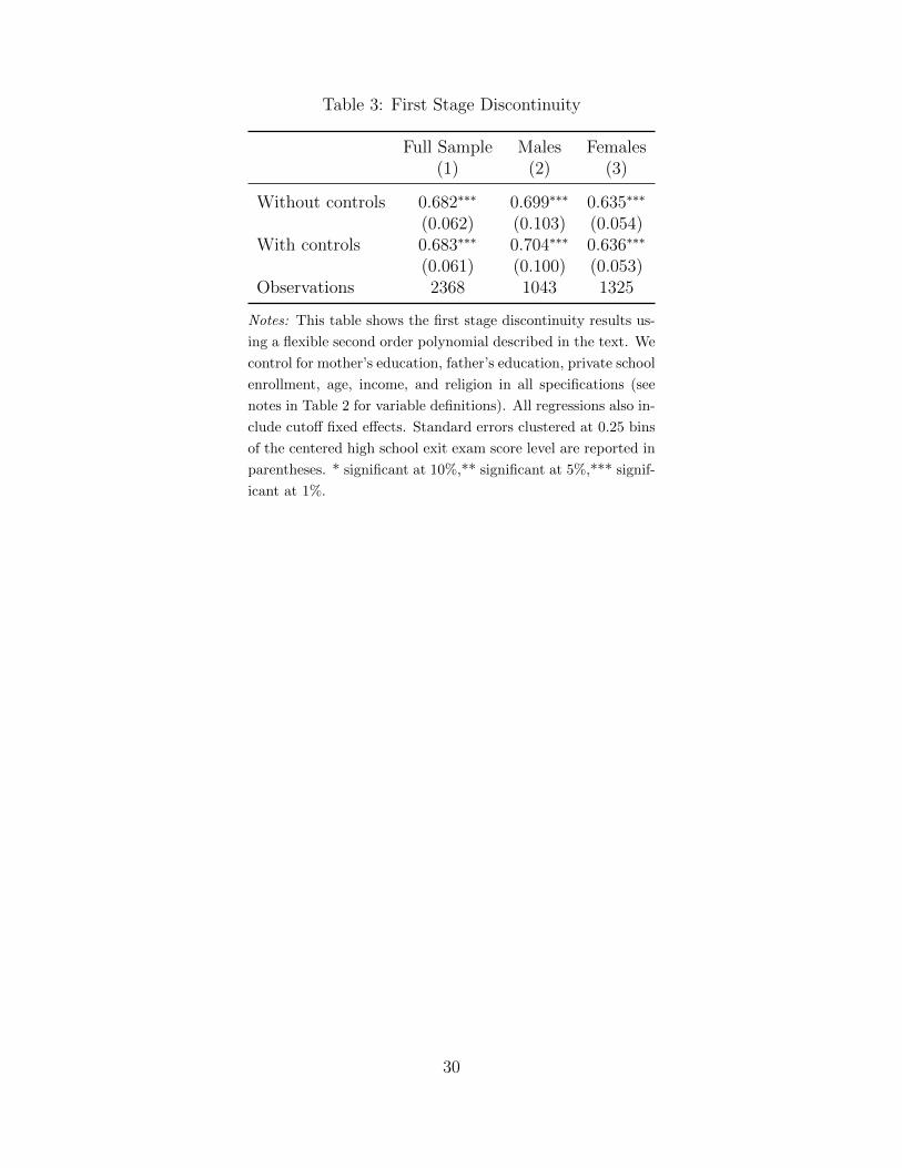
Table 3: First Stage Discontinuity
Full Sample Males Females(1) (2) (3)
Without controls 0.682∗∗∗ 0.699∗∗∗ 0.635∗∗∗
(0.062) (0.103) (0.054)With controls 0.683∗∗∗ 0.704∗∗∗ 0.636∗∗∗
(0.061) (0.100) (0.053)Observations 2368 1043 1325
Notes: This table shows the first stage discontinuity results us-
ing a flexible second order polynomial described in the text. We
control for mother’s education, father’s education, private school
enrollment, age, income, and religion in all specifications (see
notes in Table 2 for variable definitions). All regressions also in-
clude cutoff fixed effects. Standard errors clustered at 0.25 bins
of the centered high school exit exam score level are reported in
parentheses. * significant at 10%,** significant at 5%,*** signif-
icant at 1%.
30
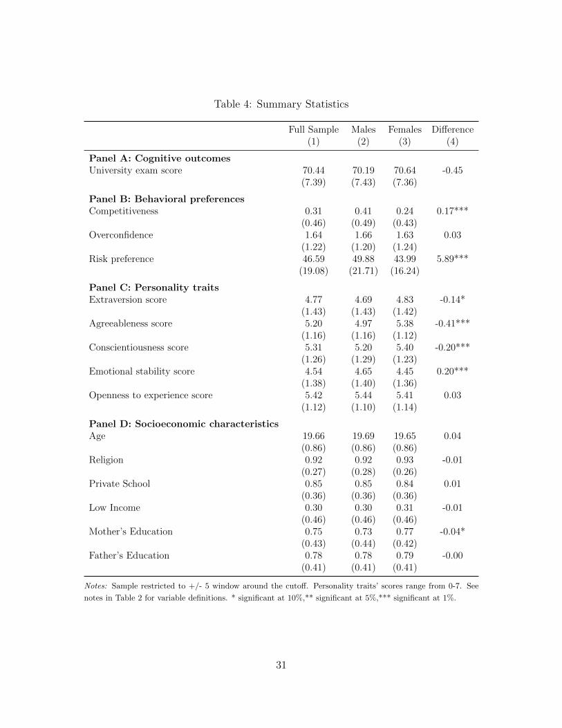
Table 4: Summary Statistics
Full Sample Males Females Difference(1) (2) (3) (4)
Panel A: Cognitive outcomesUniversity exam score 70.44 70.19 70.64 -0.45
(7.39) (7.43) (7.36)
Panel B: Behavioral preferencesCompetitiveness 0.31 0.41 0.24 0.17***
(0.46) (0.49) (0.43)Overconfidence 1.64 1.66 1.63 0.03
(1.22) (1.20) (1.24)Risk preference 46.59 49.88 43.99 5.89***
(19.08) (21.71) (16.24)
Panel C: Personality traitsExtraversion score 4.77 4.69 4.83 -0.14*
(1.43) (1.43) (1.42)Agreeableness score 5.20 4.97 5.38 -0.41***
(1.16) (1.16) (1.12)Conscientiousness score 5.31 5.20 5.40 -0.20***
(1.26) (1.29) (1.23)Emotional stability score 4.54 4.65 4.45 0.20***
(1.38) (1.40) (1.36)Openness to experience score 5.42 5.44 5.41 0.03
(1.12) (1.10) (1.14)
Panel D: Socioeconomic characteristicsAge 19.66 19.69 19.65 0.04
(0.86) (0.86) (0.86)Religion 0.92 0.92 0.93 -0.01
(0.27) (0.28) (0.26)Private School 0.85 0.85 0.84 0.01
(0.36) (0.36) (0.36)Low Income 0.30 0.30 0.31 -0.01
(0.46) (0.46) (0.46)Mother’s Education 0.75 0.73 0.77 -0.04*
(0.43) (0.44) (0.42)Father’s Education 0.78 0.78 0.79 -0.00
(0.41) (0.41) (0.41)
Notes: Sample restricted to +/- 5 window around the cutoff. Personality traits’ scores range from 0-7. See
notes in Table 2 for variable definitions. * significant at 10%,** significant at 5%,*** significant at 1%.
31
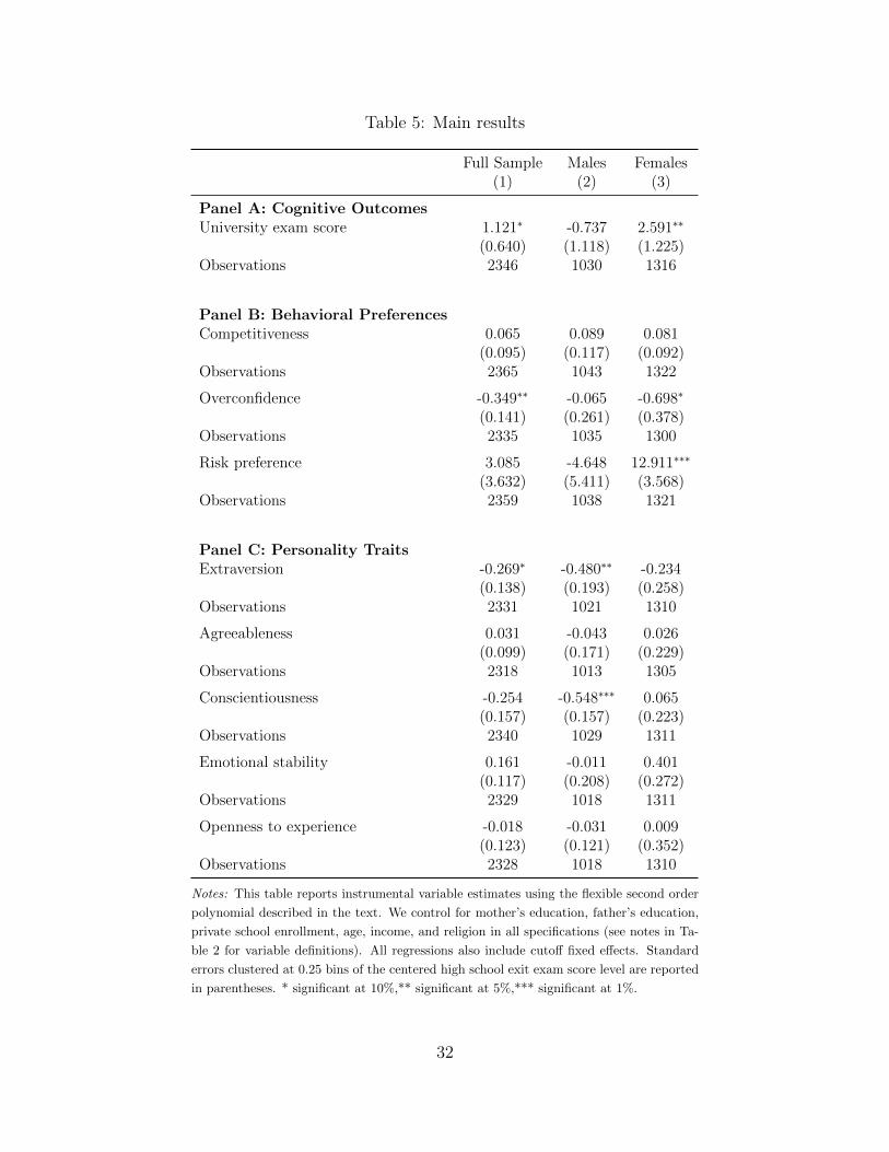
Table 5: Main results
Full Sample Males Females(1) (2) (3)
Panel A: Cognitive OutcomesUniversity exam score 1.121∗ -0.737 2.591∗∗
(0.640) (1.118) (1.225)Observations 2346 1030 1316
Panel B: Behavioral PreferencesCompetitiveness 0.065 0.089 0.081
(0.095) (0.117) (0.092)Observations 2365 1043 1322
Overconfidence -0.349∗∗ -0.065 -0.698∗
(0.141) (0.261) (0.378)Observations 2335 1035 1300
Risk preference 3.085 -4.648 12.911∗∗∗
(3.632) (5.411) (3.568)Observations 2359 1038 1321
Panel C: Personality TraitsExtraversion -0.269∗ -0.480∗∗ -0.234
(0.138) (0.193) (0.258)Observations 2331 1021 1310
Agreeableness 0.031 -0.043 0.026(0.099) (0.171) (0.229)
Observations 2318 1013 1305
Conscientiousness -0.254 -0.548∗∗∗ 0.065(0.157) (0.157) (0.223)
Observations 2340 1029 1311
Emotional stability 0.161 -0.011 0.401(0.117) (0.208) (0.272)
Observations 2329 1018 1311
Openness to experience -0.018 -0.031 0.009(0.123) (0.121) (0.352)
Observations 2328 1018 1310
Notes: This table reports instrumental variable estimates using the flexible second order
polynomial described in the text. We control for mother’s education, father’s education,
private school enrollment, age, income, and religion in all specifications (see notes in Ta-
ble 2 for variable definitions). All regressions also include cutoff fixed effects. Standard
errors clustered at 0.25 bins of the centered high school exit exam score level are reported
in parentheses. * significant at 10%,** significant at 5%,*** significant at 1%.
32
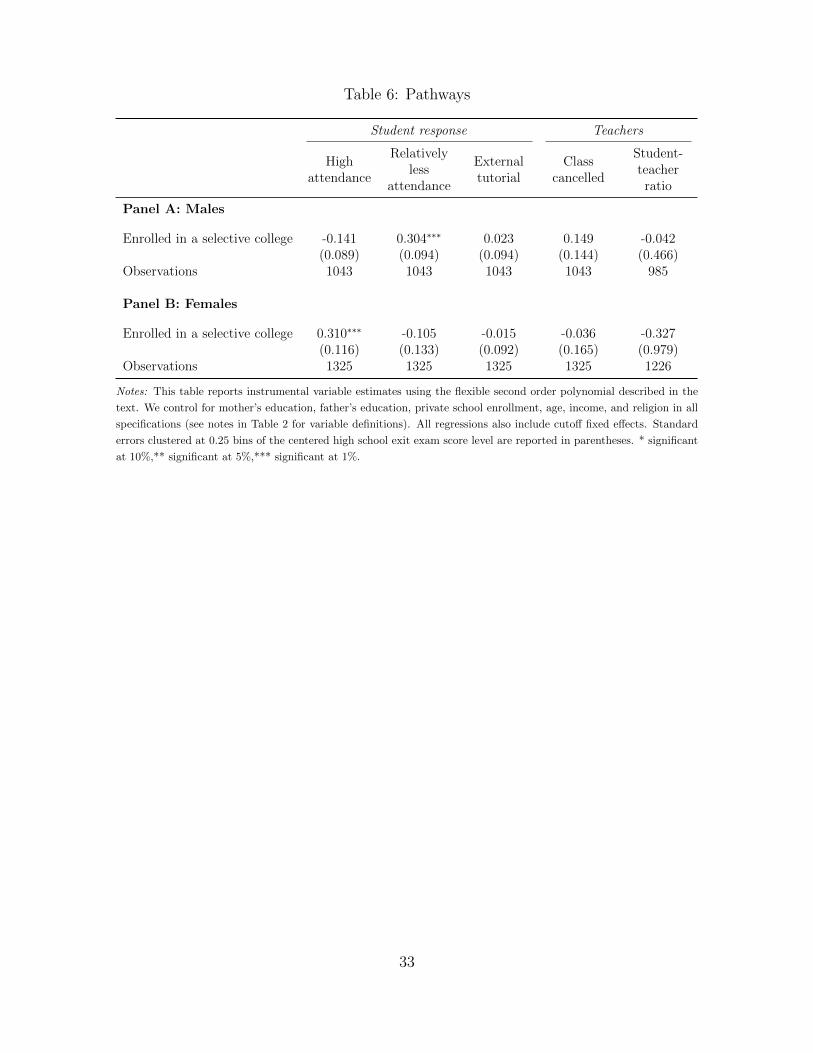
Table 6: Pathways
Student response Teachers
Highattendance
Relativelyless
attendance
Externaltutorial
Classcancelled
Student-teacherratio
Panel A: Males
Enrolled in a selective college -0.141 0.304∗∗∗ 0.023 0.149 -0.042(0.089) (0.094) (0.094) (0.144) (0.466)
Observations 1043 1043 1043 1043 985
Panel B: Females
Enrolled in a selective college 0.310∗∗∗ -0.105 -0.015 -0.036 -0.327(0.116) (0.133) (0.092) (0.165) (0.979)
Observations 1325 1325 1325 1325 1226
Notes: This table reports instrumental variable estimates using the flexible second order polynomial described in the
text. We control for mother’s education, father’s education, private school enrollment, age, income, and religion in all
specifications (see notes in Table 2 for variable definitions). All regressions also include cutoff fixed effects. Standard
errors clustered at 0.25 bins of the centered high school exit exam score level are reported in parentheses. * significant
at 10%,** significant at 5%,*** significant at 1%.
33
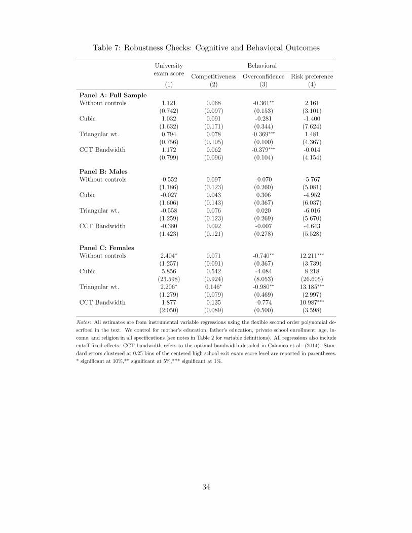
Table 7: Robustness Checks: Cognitive and Behavioral Outcomes
Universityexam score
Behavioral
Competitiveness Overconfidence Risk preference(1) (2) (3) (4)
Panel A: Full SampleWithout controls 1.121 0.068 -0.361∗∗ 2.161
(0.742) (0.097) (0.153) (3.101)Cubic 1.032 0.091 -0.281 -1.400
(1.632) (0.171) (0.344) (7.624)Triangular wt. 0.794 0.078 -0.369∗∗∗ 1.481
(0.756) (0.105) (0.100) (4.367)CCT Bandwidth 1.172 0.062 -0.379∗∗∗ -0.014
(0.799) (0.096) (0.104) (4.154)
Panel B: MalesWithout controls -0.552 0.097 -0.070 -5.767
(1.186) (0.123) (0.260) (5.081)Cubic -0.027 0.043 0.306 -4.952
(1.606) (0.143) (0.367) (6.037)Triangular wt. -0.558 0.076 0.020 -6.016
(1.259) (0.123) (0.269) (5.670)CCT Bandwidth -0.380 0.092 -0.007 -4.643
(1.423) (0.121) (0.278) (5.528)
Panel C: FemalesWithout controls 2.404∗ 0.071 -0.740∗∗ 12.211∗∗∗
(1.257) (0.091) (0.367) (3.739)Cubic 5.856 0.542 -4.084 8.218
(23.598) (0.924) (8.053) (26.605)Triangular wt. 2.206∗ 0.146∗ -0.980∗∗ 13.185∗∗∗
(1.279) (0.079) (0.469) (2.997)CCT Bandwidth 1.877 0.135 -0.774 10.987∗∗∗
(2.050) (0.089) (0.500) (3.598)
Notes: All estimates are from instrumental variable regressions using the flexible second order polynomial de-
scribed in the text. We control for mother’s education, father’s education, private school enrollment, age, in-
come, and religion in all specifications (see notes in Table 2 for variable definitions). All regressions also include
cutoff fixed effects. CCT bandwidth refers to the optimal bandwidth detailed in Calonico et al. (2014). Stan-
dard errors clustered at 0.25 bins of the centered high school exit exam score level are reported in parentheses.
* significant at 10%,** significant at 5%,*** significant at 1%.
34
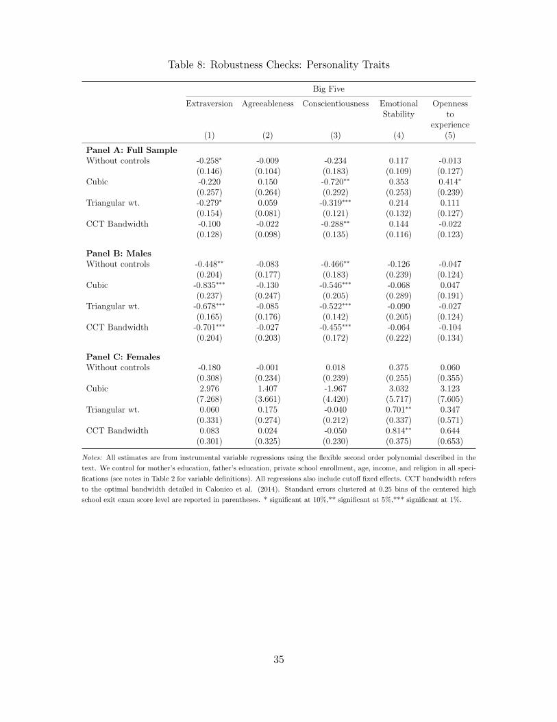
Table 8: Robustness Checks: Personality Traits
Big Five
Extraversion Agreeableness Conscientiousness EmotionalStability
Opennessto
experience(1) (2) (3) (4) (5)
Panel A: Full SampleWithout controls -0.258∗ -0.009 -0.234 0.117 -0.013
(0.146) (0.104) (0.183) (0.109) (0.127)Cubic -0.220 0.150 -0.720∗∗ 0.353 0.414∗
(0.257) (0.264) (0.292) (0.253) (0.239)Triangular wt. -0.279∗ 0.059 -0.319∗∗∗ 0.214 0.111
(0.154) (0.081) (0.121) (0.132) (0.127)CCT Bandwidth -0.100 -0.022 -0.288∗∗ 0.144 -0.022
(0.128) (0.098) (0.135) (0.116) (0.123)
Panel B: MalesWithout controls -0.448∗∗ -0.083 -0.466∗∗ -0.126 -0.047
(0.204) (0.177) (0.183) (0.239) (0.124)Cubic -0.835∗∗∗ -0.130 -0.546∗∗∗ -0.068 0.047
(0.237) (0.247) (0.205) (0.289) (0.191)Triangular wt. -0.678∗∗∗ -0.085 -0.522∗∗∗ -0.090 -0.027
(0.165) (0.176) (0.142) (0.205) (0.124)CCT Bandwidth -0.701∗∗∗ -0.027 -0.455∗∗∗ -0.064 -0.104
(0.204) (0.203) (0.172) (0.222) (0.134)
Panel C: FemalesWithout controls -0.180 -0.001 0.018 0.375 0.060
(0.308) (0.234) (0.239) (0.255) (0.355)Cubic 2.976 1.407 -1.967 3.032 3.123
(7.268) (3.661) (4.420) (5.717) (7.605)Triangular wt. 0.060 0.175 -0.040 0.701∗∗ 0.347
(0.331) (0.274) (0.212) (0.337) (0.571)CCT Bandwidth 0.083 0.024 -0.050 0.814∗∗ 0.644
(0.301) (0.325) (0.230) (0.375) (0.653)
Notes: All estimates are from instrumental variable regressions using the flexible second order polynomial described in the
text. We control for mother’s education, father’s education, private school enrollment, age, income, and religion in all speci-
fications (see notes in Table 2 for variable definitions). All regressions also include cutoff fixed effects. CCT bandwidth refers
to the optimal bandwidth detailed in Calonico et al. (2014). Standard errors clustered at 0.25 bins of the centered high
school exit exam score level are reported in parentheses. * significant at 10%,** significant at 5%,*** significant at 1%.
35
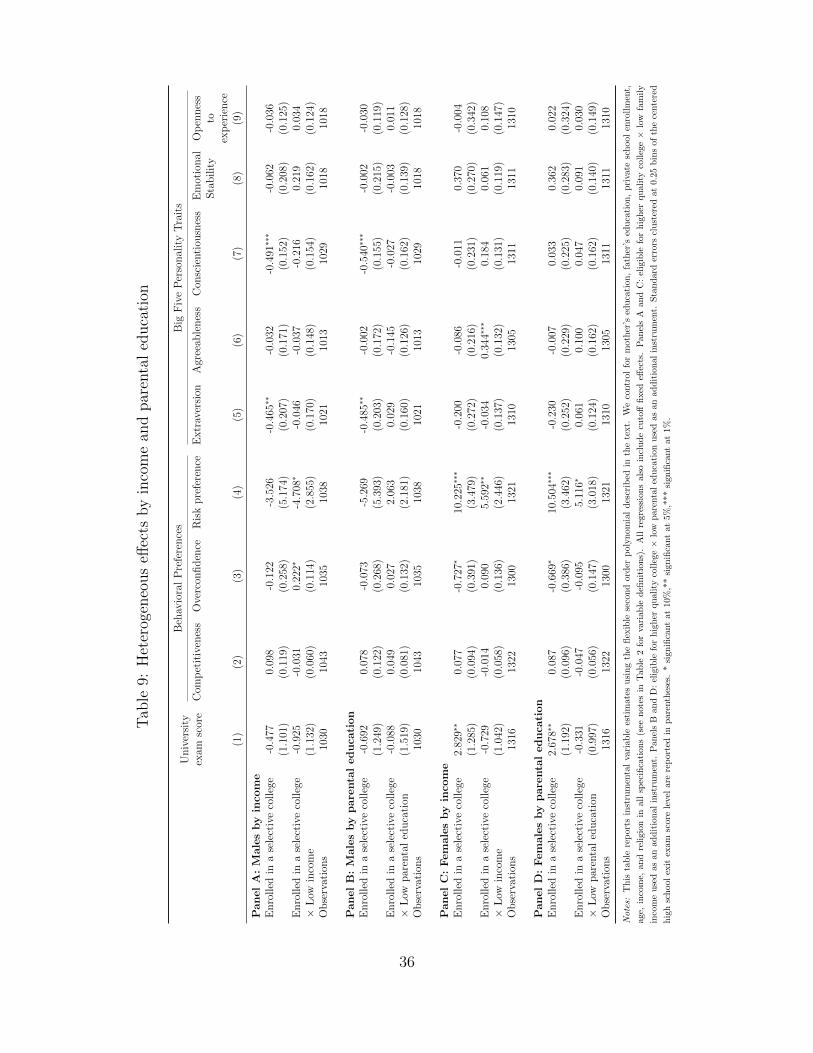
Tab
le9:
Het
erog
eneo
us
effec
tsby
inco
me
and
par
enta
led
uca
tion
Univ
ersi
tyex
amsc
ore
Beh
avio
ral
Pre
fere
nce
sB
igF
ive
Per
sonal
ity
Tra
its
Com
pet
itiv
enes
sO
verc
onfiden
ceR
isk
pre
fere
nce
Extr
aver
sion
Agr
eeab
lenes
sC
onsc
ienti
ousn
ess
Em
otio
nal
Sta
bilit
yO
pen
nes
sto
exp
erie
nce
(1)
(2)
(3)
(4)
(5)
(6)
(7)
(8)
(9)
Pan
el
A:
Male
sby
inco
me
Enro
lled
ina
sele
ctiv
eco
lleg
e-0
.477
0.09
8-0
.122
-3.5
26-0
.465∗∗
-0.0
32-0
.491∗∗∗
-0.0
62-0
.036
(1.1
01)
(0.1
19)
(0.2
58)
(5.1
74)
(0.2
07)
(0.1
71)
(0.1
52)
(0.2
08)
(0.1
25)
Enro
lled
ina
sele
ctiv
eco
lleg
e-0
.925
-0.0
310.
222∗
-4.7
08∗
-0.0
46-0
.037
-0.2
160.
219
0.03
4×
Low
inco
me
(1.1
32)
(0.0
60)
(0.1
14)
(2.8
55)
(0.1
70)
(0.1
48)
(0.1
54)
(0.1
62)
(0.1
24)
Obse
rvat
ions
1030
1043
1035
1038
1021
1013
1029
1018
1018
Pan
el
B:
Male
sby
pare
nta
led
uca
tion
Enro
lled
ina
sele
ctiv
eco
lleg
e-0
.692
0.07
8-0
.073
-5.2
69-0
.485∗∗
-0.0
02-0
.540∗∗∗
-0.0
02-0
.030
(1.2
49)
(0.1
22)
(0.2
68)
(5.3
93)
(0.2
03)
(0.1
72)
(0.1
55)
(0.2
15)
(0.1
19)
Enro
lled
ina
sele
ctiv
eco
lleg
e-0
.088
0.04
90.
027
2.06
30.
029
-0.1
45-0
.027
-0.0
030.
011
×L
owpar
enta
led
uca
tion
(1.5
19)
(0.0
81)
(0.1
32)
(2.1
81)
(0.1
60)
(0.1
26)
(0.1
62)
(0.1
39)
(0.1
28)
Obse
rvat
ions
1030
1043
1035
1038
1021
1013
1029
1018
1018
Pan
el
C:
Fem
ale
sby
inco
me
Enro
lled
ina
sele
ctiv
eco
lleg
e2.
829∗∗
0.07
7-0
.727∗
10.2
25∗∗∗
-0.2
00-0
.086
-0.0
110.
370
-0.0
04(1
.285
)(0
.094
)(0
.391
)(3
.479
)(0
.272
)(0
.216
)(0
.231
)(0
.270
)(0
.342
)E
nro
lled
ina
sele
ctiv
eco
lleg
e-0
.729
-0.0
140.
090
5.59
2∗∗
-0.0
340.
344∗∗∗
0.18
40.
061
0.10
8×
Low
inco
me
(1.0
42)
(0.0
58)
(0.1
36)
(2.4
46)
(0.1
37)
(0.1
32)
(0.1
31)
(0.1
19)
(0.1
47)
Obse
rvat
ions
1316
1322
1300
1321
1310
1305
1311
1311
1310
Pan
el
D:
Fem
ale
sby
pare
nta
led
uca
tion
Enro
lled
ina
sele
ctiv
eco
lleg
e2.
678∗∗
0.08
7-0
.669∗
10.5
04∗∗∗
-0.2
30-0
.007
0.03
30.
362
0.02
2(1
.192
)(0
.096
)(0
.386
)(3
.462
)(0
.252
)(0
.229
)(0
.225
)(0
.283
)(0
.324
)E
nro
lled
ina
sele
ctiv
eco
lleg
e-0
.331
-0.0
47-0
.095
5.11
6∗0.
061
0.10
00.
047
0.09
10.
030
×L
owpar
enta
led
uca
tion
(0.9
97)
(0.0
56)
(0.1
47)
(3.0
18)
(0.1
24)
(0.1
62)
(0.1
62)
(0.1
40)
(0.1
49)
Obse
rvat
ions
1316
1322
1300
1321
1310
1305
1311
1311
1310
Notes:
This
table
rep
orts
inst
rum
enta
lva
riab
lees
tim
ates
usi
ng
the
flex
ible
seco
nd
ord
erp
olynom
ial
des
crib
edin
the
text.
We
contr
olfo
rm
oth
er’s
educa
tion,
fath
er’s
educa
tion,
pri
vate
school
enro
llm
ent,
age,
inco
me,
and
religi
onin
all
spec
ifica
tion
s(s
eenot
esin
Table
2fo
rva
riab
ledefi
nit
ions)
.A
llre
gre
ssio
ns
als
oin
clude
cuto
fffixed
effec
ts.
Panel
sA
and
C:
elig
ible
for
hig
her
quality
colleg
e×
low
fam
ily
inco
me
use
das
anad
dit
ional
inst
rum
ent.
Pan
els
Ban
dD
:el
igib
lefo
rhig
her
quality
colleg
e×
low
pare
nta
led
uca
tion
use
das
an
addit
ional
inst
rum
ent.
Sta
ndard
erro
rscl
ust
ered
at0.2
5bin
sof
the
cente
red
hig
hsc
hool
exit
exam
scor
ele
vel
are
rep
orte
din
par
enth
eses
.*
sign
ifica
nt
at10%
,**
signifi
cant
at5%
,***
sign
ifica
nt
at
1%.
36
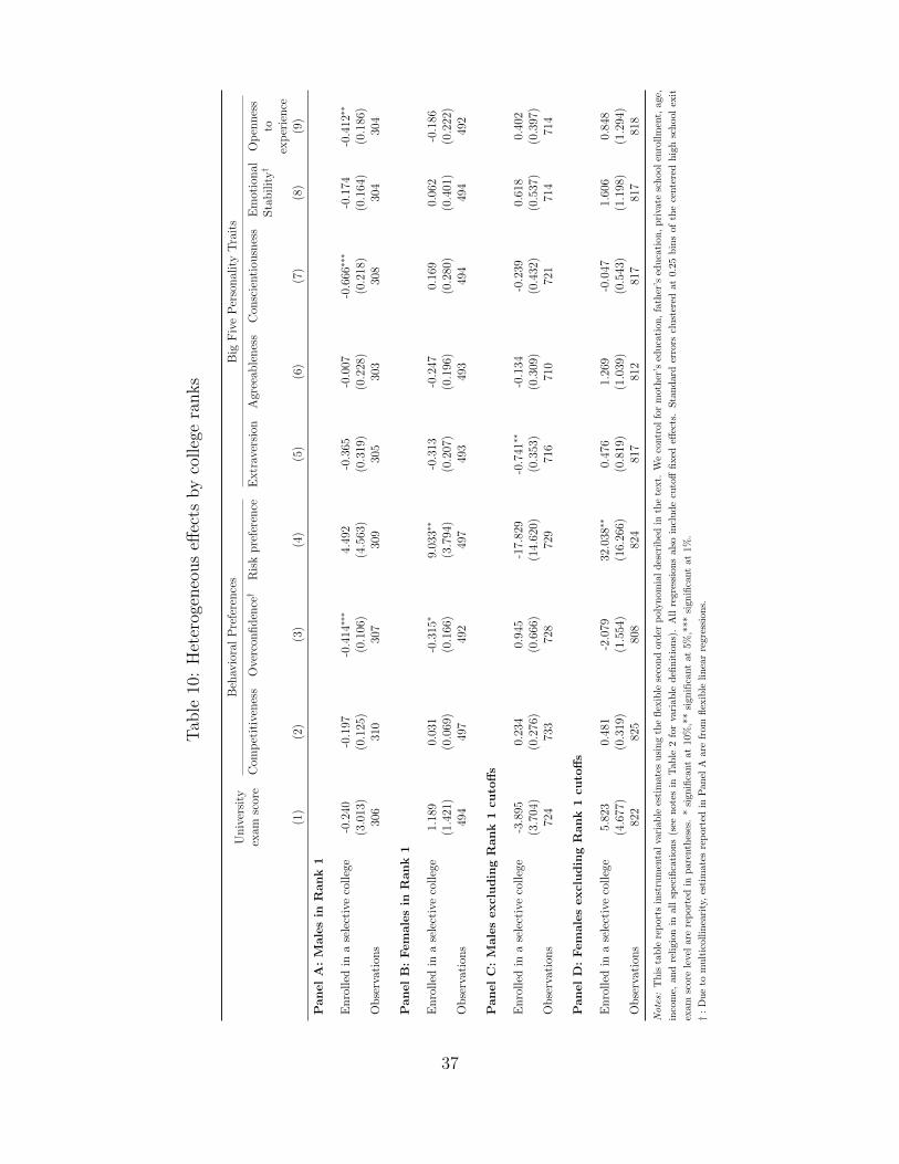
Tab
le10
:H
eter
ogen
eous
effec
tsby
colleg
era
nks
Univ
ersi
tyex
amsc
ore
Beh
avio
ral
Pre
fere
nce
sB
igF
ive
Per
sonal
ity
Tra
its
Com
pet
itiv
enes
sO
verc
onfiden
ce†
Ris
kpre
fere
nce
Extr
aver
sion
Agr
eeab
lenes
sC
onsc
ienti
ousn
ess
Em
otio
nal
Sta
bilit
y†
Op
ennes
sto
exp
erie
nce
(1)
(2)
(3)
(4)
(5)
(6)
(7)
(8)
(9)
Pan
el
A:
Male
sin
Ran
k1
Enro
lled
ina
sele
ctiv
eco
lleg
e-0
.240
-0.1
97-0
.414∗∗∗
4.49
2-0
.365
-0.0
07-0
.666∗∗∗
-0.1
74-0
.412∗∗
(3.0
13)
(0.1
25)
(0.1
06)
(4.5
63)
(0.3
19)
(0.2
28)
(0.2
18)
(0.1
64)
(0.1
86)
Obse
rvat
ions
306
310
307
309
305
303
308
304
304
Pan
el
B:
Fem
ale
sin
Ran
k1
Enro
lled
ina
sele
ctiv
eco
lleg
e1.
189
0.03
1-0
.315∗
9.03
3∗∗
-0.3
13-0
.247
0.16
90.
062
-0.1
86(1
.421
)(0
.069
)(0
.166
)(3
.794
)(0
.207
)(0
.196
)(0
.280
)(0
.401
)(0
.222
)O
bse
rvat
ions
494
497
492
497
493
493
494
494
492
Pan
el
C:
Male
sexcl
ud
ing
Ran
k1
cuto
ffs
Enro
lled
ina
sele
ctiv
eco
lleg
e-3
.895
0.23
40.
945
-17.
829
-0.7
41∗∗
-0.1
34-0
.239
0.61
80.
402
(3.7
04)
(0.2
76)
(0.6
66)
(14.
620)
(0.3
53)
(0.3
09)
(0.4
32)
(0.5
37)
(0.3
97)
Obse
rvat
ions
724
733
728
729
716
710
721
714
714
Pan
el
D:
Fem
ale
sexcl
ud
ing
Ran
k1
cuto
ffs
Enro
lled
ina
sele
ctiv
eco
lleg
e5.
823
0.48
1-2
.079
32.0
38∗∗
0.47
61.
269
-0.0
471.
606
0.84
8(4
.677
)(0
.319
)(1
.554
)(1
6.26
6)(0
.819
)(1
.039
)(0
.543
)(1
.198
)(1
.294
)O
bse
rvat
ions
822
825
808
824
817
812
817
817
818
Notes:
This
table
rep
orts
inst
rum
enta
lva
riab
lees
tim
ates
usi
ng
the
flex
ible
seco
nd
order
poly
nom
ial
des
crib
edin
the
text.
We
contr
ol
for
moth
er’s
educa
tion,
fath
er’s
educa
tion
,pri
vate
school
enro
llm
ent,
age,
inco
me,
and
religi
onin
all
spec
ifica
tion
s(s
eenot
esin
Tab
le2
for
vari
able
defi
nit
ions)
.A
llre
gre
ssio
ns
als
oin
clude
cuto
fffixed
effec
ts.
Sta
ndard
erro
rscl
ust
ered
at0.
25
bin
sof
the
cente
red
hig
hsc
hool
exit
exam
scor
ele
vel
are
rep
orte
din
par
enth
eses
.*
sign
ifica
nt
at10
%,*
*si
gnifi
cant
at5%
,***
signifi
cant
at
1%.
†:
Due
tom
ult
icol
linea
rity
,es
tim
ates
rep
orte
din
Pan
elA
are
from
flex
ible
linea
rre
gres
sion
s.
37
Online appendix for:
Cognitive, Socioemotional and Behavioral Returns toCollege Quality
UTTEEYO DASGUPTA, SUBHA MANI, SMRITI SHARMA, SAURABH SINGHAL
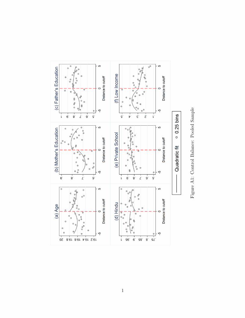
Fig
ure
A1:
Con
trol
Bal
ance
:P
ool
edSam
ple
1
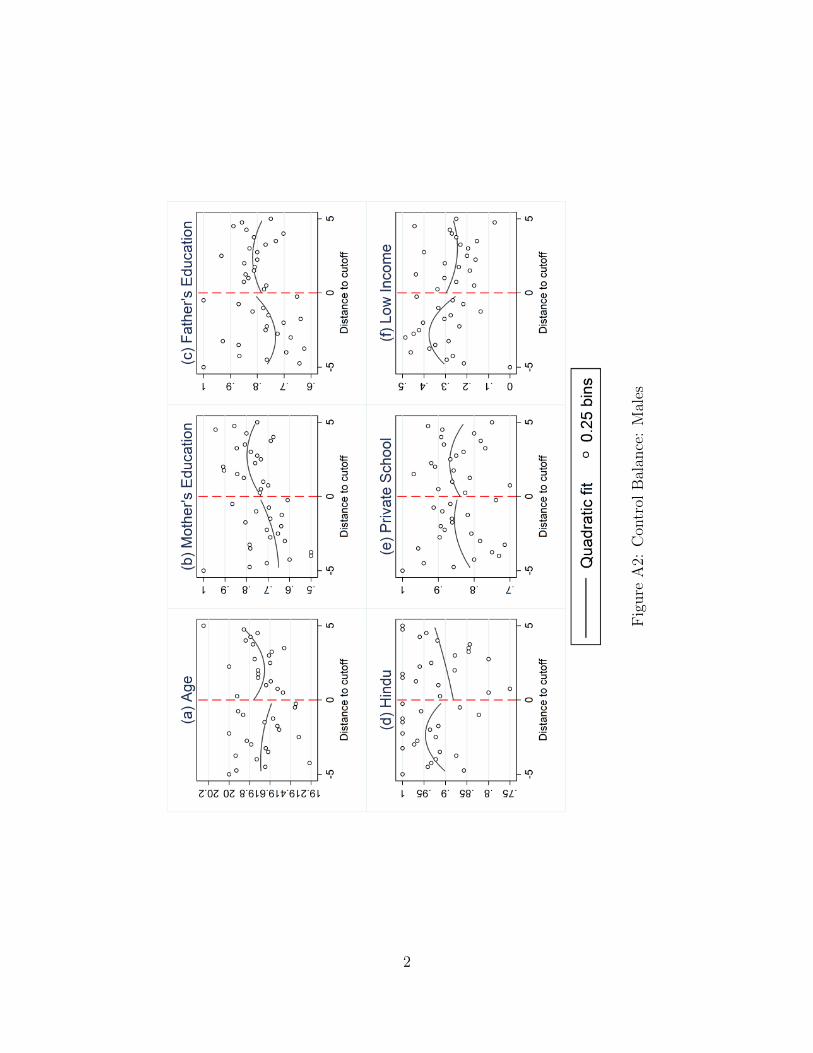
Fig
ure
A2:
Con
trol
Bal
ance
:M
ales
2
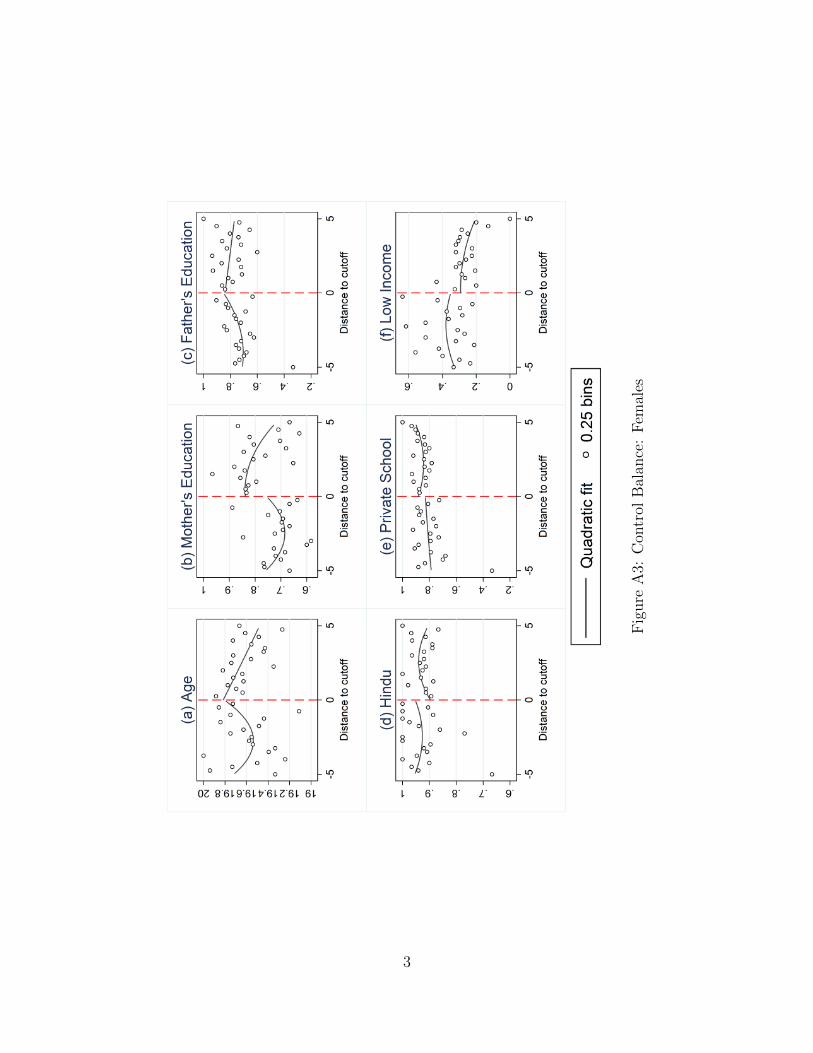
Fig
ure
A3:
Con
trol
Bal
ance
:F
emal
es
3
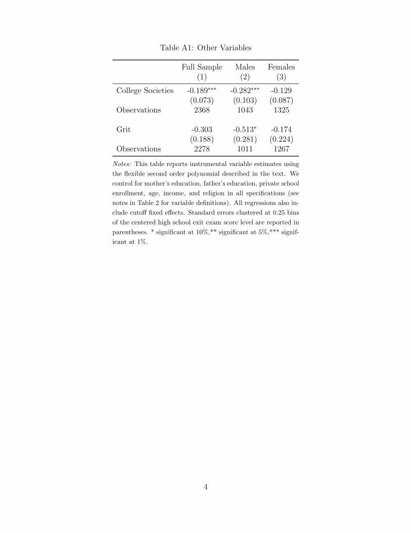
Table A1: Other Variables
Full Sample Males Females(1) (2) (3)
College Societies -0.189∗∗∗ -0.282∗∗∗ -0.129(0.073) (0.103) (0.087)
Observations 2368 1043 1325
Grit -0.303 -0.513∗ -0.174(0.188) (0.281) (0.224)
Observations 2278 1011 1267
Notes: This table reports instrumental variable estimates using
the flexible second order polynomial described in the text. We
control for mother’s education, father’s education, private school
enrollment, age, income, and religion in all specifications (see
notes in Table 2 for variable definitions). All regressions also in-
clude cutoff fixed effects. Standard errors clustered at 0.25 bins
of the centered high school exit exam score level are reported in
parentheses. * significant at 10%,** significant at 5%,*** signif-
icant at 1%.
4
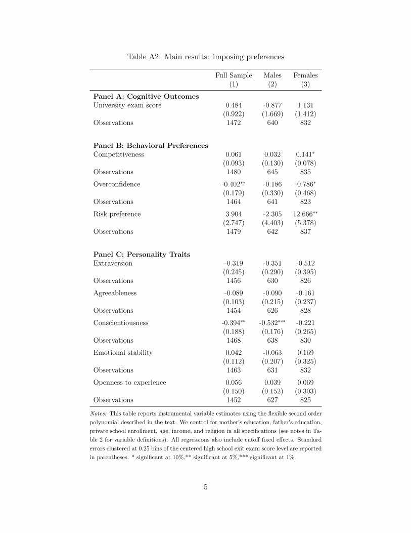
Table A2: Main results: imposing preferences
Full Sample Males Females(1) (2) (3)
Panel A: Cognitive OutcomesUniversity exam score 0.484 -0.877 1.131
(0.922) (1.669) (1.412)Observations 1472 640 832
Panel B: Behavioral PreferencesCompetitiveness 0.061 0.032 0.141∗
(0.093) (0.130) (0.078)Observations 1480 645 835
Overconfidence -0.402∗∗ -0.186 -0.786∗
(0.179) (0.330) (0.468)Observations 1464 641 823
Risk preference 3.904 -2.305 12.666∗∗
(2.747) (4.403) (5.378)Observations 1479 642 837
Panel C: Personality TraitsExtraversion -0.319 -0.351 -0.512
(0.245) (0.290) (0.395)Observations 1456 630 826
Agreeableness -0.089 -0.090 -0.161(0.103) (0.215) (0.237)
Observations 1454 626 828
Conscientiousness -0.394∗∗ -0.532∗∗∗ -0.221(0.188) (0.176) (0.265)
Observations 1468 638 830
Emotional stability 0.042 -0.063 0.169(0.112) (0.207) (0.325)
Observations 1463 631 832
Openness to experience 0.056 0.039 0.069(0.150) (0.152) (0.303)
Observations 1452 627 825
Notes: This table reports instrumental variable estimates using the flexible second order
polynomial described in the text. We control for mother’s education, father’s education,
private school enrollment, age, income, and religion in all specifications (see notes in Ta-
ble 2 for variable definitions). All regressions also include cutoff fixed effects. Standard
errors clustered at 0.25 bins of the centered high school exit exam score level are reported
in parentheses. * significant at 10%,** significant at 5%,*** significant at 1%.
5


![[FOR ONLINE PUBLICATION] Web Appendix to “Socioemotional](https://img.pdfslide.us/doc/110x75/620c61ae8ae115289c66c73e/for-online-publication-web-appendix-to-socioemotional-.jpg)