Embed Size (px)
Citation preview
Why do Firms Hold Oil Stockpiles?
Charles F. Mason†
H.A. True Chair in Petroleum and Natural Gas EconomicsDepartment of Economics & Finance
University of Wyoming,1000 E. University Ave.
Laramie, WY 82071
March 31, 2009
Abstract
Persistent and significant privately-held stockpiles of crude oil have long been an im-portant empirical regularity in the United States. Such stockpiles would not rationallybe held in a traditional Hotelling-style model. How then can the existence of these in-ventories be explained? In the presence of sufficiently stochastic prices, oil extractingfirms have an incentive to hold inventories to smooth production over time. An alter-native explanation is related to a speculative motive - firms hold stockpiles intending tocash in on periods of particularly high prices. I argue that empirical evidence supportsthe former but not the latter explanation.
Keywords: Petroleum Economics, Stochastic Dynamic Optimization
JEL Areas: Q2, D8, L15
†phone: +1-307-766-2178; fax: +1-307-766-5090; e-mail: [email protected]
1 Introduction
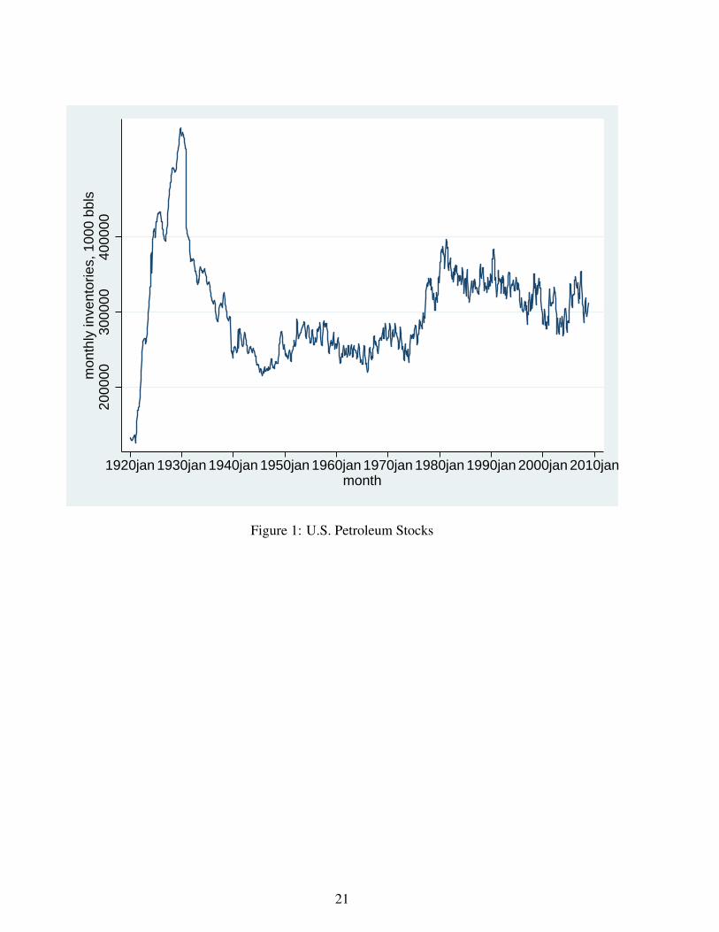
Since official records were first kept in the United States (U.S.), in 1920, private interests have
consistently held significant inventories of crude oil. Over the course of the past few decades, these
inventories have averaged around 325 million barrels. While these holdings have fluctuated some
they have been remarkably persistent over the past 70 years, ranging from just over 215 million
barrels to slightly less than 398 million barrels (see Figure 1). What motivates these substantial
inventory holdings? One answer is that stockpiles could be held for speculative purposes – betting
on abnormally rapid price run-ups. An alternative explanation is that petroleum extracting firms
would like to hedge against substantial swings in extraction costs.1
Neither explanation is compelling in a deterministic setting. In a deterministic world prices
would have to rise at the rate of interest to induce firms to hold stockpiles. But if prices increased at
the rate of interest, rents would typically rise faster than the interest rate. Firms would then prefer
to delay extraction, so that there would be no fodder from which to build inventories. The answer,
I believe, must lie in fluctuating prices.
Reacting to the volatile changes in petroleum prices during the past year, some key players
in OPEC and a number of members of the U.S. Congress placed the blame on speculators. One
issue left unanswered in this dialog was the role of privately held inventories. If speculation was
at play, one would expect resource inventory holders to cash in on abnormally high prices. As I
discuss below, while there was a negative correlation between spot prices and inventory holdings,
prices only explain a paltry amount of the variation in inventories. Indeed, inventories did not
change much even when prices increased or decreased dramatically, as during this past year. It
seems likely that some other effect played a more important role.
1
An alternative, and I believe compelling, motivation is related to the concept of production
smoothing (Arrow et al. (1958), Blanchard and Fisher (1989)). If oil prices are driven by a random
process, perhaps arising from demand shocks, the induced fluctuations in market price will lead to
variations in the firm’s optimal extraction rate. So long as there is enough variation in production,
relative to the overall downward trend in production that must occur for non-renewable resources,
and so long as it is costly to expand production, firms will wish to hold inventories to guard against
future cost increases. This explanation will hold true no matter what current price is, and no matter
what the current level of resources in situ.
In this paper I explore the implication of such motivations. I start by discussing the con-
ceptual underpinnings of the story in section 2, formally demonstrating that a resource extracting
firm would generally not acquire stockpiles in a deterministic world. I then analyze a version of
the model allowing for stochastic prices in section 3. I turn to an examination of the data in section
4. Here I argue that the variation in spot prices has been sufficient to motivate the acquisition of
inventories for almost all months during the past two decades. By contrast, I find that the impact
of spot prices upon both levels of and changes in privately-held oil stocks is modest at best. I
conclude with a discussion of potential extensions of the model in section 5.
2 Deterministic Prices and the Incentive to Stockpile
Consider a price-taking firm engaged in the extraction of oil. The firm in question has an initial
deposit of the resource of size R0, from which it may choose to extract. Its rate of extraction is
yt , and its rate of sales, qt , are selected to maximize the discounted flow of its profits. It will be
convenient to adjust the firm’s problem slightly, and use net additions to inventories, wt = yt −qt ,
2
as a control variable in place of sales.
The firm’s reserves at instant t are Rt and its inventory holdings are St . I assume the firm
starts with no inventories. Reserves decumulate with extraction, while inventories accumulate
according to the difference between extraction and sales:
Rt = −yt ; (1)
St = wt . (2)
When it is actively extracting, the firm bears positive operating costs. I assume marginal
extraction costs are positive, upward-sloping and weakly convex, with both total costs and marginal
costs decreasing in R. A simple example of a cost function that has these features is
c(y,R) = A0 +A1yη/R, (3)
which is adapted from Pindyck (1980). This function, which combines flow fixed costs with a
power function of the rate of extraction that is proportional to the inverse of reserves, has two de-
sirable features: There is a range of falling average extraction costs, and extraction becomes more
costly the greater is the ratio of extraction to reserves; both aspects are consistent with anecdotal
evidence. In this functional form, η−1 can be interpreted as the elasticity of marginal extraction
cost with respect to the rate of extraction. The assumption of weakly convex marginal costs implies
η ≥ 2. For now, I assume that it is costless to hold inventories; the implications of relaxing this
assumption are discussed below.
3
Denoting the market price of oil at instant t by Pt , the instantaneous rate of profits is
πt = Pt [yt −wt ]− c(yt ,Rt). (4)
The goal is to select time paths of y and w so as to maximize the present discounted value of the
flow of profits.
The firm’s current value Hamiltonian is
H = Pt(yt −wt)− c(yt ,Rt)−λtyt +µtwt ,
where λt and µt are the current-value shadow prices of reserves and inventories, respectively. Pon-
tryagin’s maximum condition gives the necessary conditions for optimization:
Pt − ∂c∂y−λt = 0; (5)
Pt −µt
> 0 ⇒ wt =−∞ if St > 0; wt = 0 if St = 0
= 0 ⇒ wt is indeterminate.
< 0 ⇒ wt = yt
(6)
In principle, it is possible for the firm to liquidate some of its inventories by choosing w =−∞. As
such action would radically depress market price it can be ruled out by market clearing. On the
other hand, if the firm does not hold inventories then w ≥ 0 (i.e., there are no inventories to sell
from). Moreover, since as a general rule oil firms do not stockpile all their extraction, it seems the
first branch is empirically implausible. I therefore proceed assuming the firm’s optimal time path
4
of w is based on the middle branch of (6), unless it never pays to acquire inventories.2
In addition to the first-order conditions above, the solution must satisfy the equations of
motion for the shadow values:
λ = rλ+∂c∂R
; (7)
µ = rµ; (8)
where r is the interest rate. It is apparent that the solution to the differential equation governing µ
is an exponential, with that shadow value growing at the rate r.
If the firm is actively extracting over an interval of time then one may time-differentiate eq.
(5). Then combining with eq. (7), one obtains
d[Pt − ∂c∂y
]/dt = λ = r[Pt − ∂c∂y
]+∂c∂R
, or
[Pt/Pt − r
]Pt = d[
∂c∂y
]/dt− r∂c∂y
+∂c∂R
. (9)
Suppose now that the firm finds it optimal to add to inventories over a period of time. Then
the middle branch of eq. (6) applies; time-differentiating and combining with eq. (8), one infers
that price would then rise at the rate of interest. The conclusion is that prices must increase at the
rate of interest for the firm to be willing to add to inventories. But eq. (9) then implies
d[∂c∂y
]/dt− r∂c∂y
+∂c∂R
= 0⇐⇒
(∂2c/∂y2)y− (∂2c/∂y∂R)y− r∂c∂y
+∂c∂R
= 0.
5
With the particular functional form in eq. (3), this condition reduces to
y/y =r
η−1− y
ηR. (10)
If this simple relation fails the firm will either sell all or none of its extracted oil. Since as a general
rule oil firms do not stockpile all their extraction, it seems the empirically likely outcomes are
either stockpiling (if eq. (10) holds) or no stockpiling (if it does not).
Intuitively, if the firm were to hold stockpiles, it would possess two classes of stocks,
inventories and in situ reserves. These stocks differ in terms of their extraction costs: inventories
can be costlessly used (since the extraction costs have already been paid), while reserves in the
ground are costly to extract. In this case, the optimal program must use up the lower cost reserves
first. However, the only way inventories could exist in the first place is if excess extraction were to
occur at some point in time, and so it follows that no inventories would ever be held.
It is worth reiterating that prices are deterministic in this context – i.e., the entire price path
is known. What is the implication of relaxing this assumption, allowing for stochastic prices?
3 A Model With Stochastic Prices
Now suppose that the spot price of oil follows a random process, where the fluctuations in price
result from demand-side shocks. For concreteness I take this random process to be geometric
Brownian motion:3
dPt/Pt = µdt +σdz, (11)
6
where dz is an increment from a standard Wiener process. Convergence of the model requires that
the trend in prices does not exceed r, the firm’s discount rate: µ < r.
The nature of the firm’s decision problem is similar to those studied by Pindyck (1980,
1982). At each instant the firm’s decision problem is governed by the level of its reserves, its
inventories and market price. For expositional simplicity I assume the firm chooses to actively
extract over the time horizon in question; allowing for the possibility the firm might wish to cease
extraction, or re-activate extraction, can be readily incorporated, though at the cost of some extra
complexity.4
Let V (t,Rt ,St ,Pt) denote the optimal value function when the firm is currently active at
instant t, with in situ reserves of Rt , inventories of St and market price equal to Pt . The fundamental
equation of optimality for a currently active firm is (Kamien and Schwartz, 1991):
max yt ,wt
{πte−rt +∂V/∂t− yt∂V/∂R+wt∂V/∂S +µPt∂V/∂P+(σP
t /)∂V/∂P}
= 0. (12)
As in the deterministic case, the optimal extraction rate balances current rents against the shadow
price of reserves in situ, for a firm that actively extracts at instant t:
Pt − ∂c∂y
(y∗t ,Rt)−∂V/∂R = 0, (13)
where y∗t solves the maximization problem in (12). Also as in the deterministic case, the maximand
in (12) is linear in wt . Thus, optimal adjustments to inventories satisfy
−Pt +∂V/∂S≥ 0. (14)
7
If the shadow value of inventories is larger than current price, all production is allocated to inven-
tories; if Pt = ∂V/∂S, then wt is indeterminate.5
It is instructive to think of the firm as solving a sequence of problems. At each instant t,
the firm determines an optimal program, based on the current (and observed) demand shock. This
consists of extraction and inventory plans for each future instant that maximize the discounted
expected flow of profits, conditional on current demand, where the expectation is with respect
to the future stream of prices. This program is subject to the anticipation that reserves will be
exhausted at the terminal moment (Pindyck, 1980). Then in the next instant, a new demand shock
is observed and the firm re-optimizes.
In the analysis I conducted within the deterministic framework, the next step was to time-
differentiate the condition governing the optimal extraction rate. Here, however, the optimal ex-
traction rate will generally be a function of the stochastic variable P, as will the marginal value of
reserves. As a result, there is no proper time derivative for either side of eq. (13). The stochastic
analog of the time derivative, Ito’s differential operator, 1dtE
[d(•)], is used in its place (Kamien
and Schwartz, 1991). Applying this operator to eq. (13) yields:
1dt
E[d(P)
]− 1dt
E[d(
∂c∂y
)]=
1dt
E[d(∂V/∂R)
], (15)
where I have omitted the time subscript where there will be no confusion.
In the deterministic case, one expects the time rate of change in marginal costs to be smaller
than the present value of current marginal cost.6 Unlike the deterministic case, however, marginal
costs can rise over time in the context of stochastic demand. Despite the overall tendency for pro-
duction to decline over time, on average, the stochastic nature of extraction can yield an increase in
8
anticipated marginal cost if the variation in extraction is sufficiently large, relative to the slope of
marginal costs. This occurs because the optimal extraction rate is subject to a stochastic influence,
which in turn means that marginal extraction cost will typically fluctuate. If there is enough vari-
ation in the demand shock, this more than compensates for the reductions in extraction that will
occur on average.
From the discussion above, if the firm is to be willing to hold inventories then it must be the
case that Pt = ∂V/∂S. The analysis leading up to equation (12) in Pindyck (1980) can be applied
here to show that 1dtE
[d(∂V/∂S)
]= r∂V/∂S. It follows that a necessary condition for the firm to
be willing to stockpile oil is
1dt
E[d(P)
]= rP. (16)
Intuitively, a firm holding a barrel of stockpiled oil has the option of selling it at instant
t or holding it for a brief period, and obtaining a capital gain. The opportunity cost of holding
the inventory is the capitalized value of foregone sales, rP, while the expected capital gain is
1dtE
[d(P)
]. If the latter is not smaller than the former, there will be an incentive to stockpile some
ore (Pindyck, 1980, 1982). In light of eqs. (13), (15) and (16), it is apparent that there will be an
incentive to stockpile oil when the anticipated rate of change in marginal extraction cost just equals
the capitalized level of marginal cost:
1dt
E[d(
∂c∂y
)]= r
∂c∂y
.
I show in the appendix that this condition corresponds to
9
−y(∂2c
∂y2∂y∂R
+∂2c
∂y∂R
)+
σ2P2
2
[ ∂2y∂P2
∂2c∂y2 +
∂3c∂y3 (
∂y∂P
)2]− r
∂c∂y
= 0. (17)
It may seem counter-intuitive that a firm holding both reserves and inventories would be
willing to simultaneously extract and stockpile, as in situ reserves are higher cost to develop than
are stockpiles. Indeed, such simultaneous activities cannot be part of an optimal program under
deterministic conditions. But this need not be the case in a stochastic environment. In particular, it
can pay the firm to use up its higher cost reserves first, holding the lower cost reserves until a later
date when demand is stochastic (Slade, 1988). This is one interpretation of behavior in my model:
firms hold onto the lower cost inventory reserves, electing not to sell them until after the higher
cost (in situ) reserves are exhausted.7
To make further headway, I assume that extraction costs are given by the specific functional
form in eq. (3), with η = 2.8 Incorporating this specific form into eq. (17) and simplifying yields
∂c∂y
{ yR− ∂y
∂R+
(σ2P2
2y
) ∂2y∂P2 − r
}= 0, or
yR− ∂y
∂R+
(σ2P2
2y
) ∂2y∂P2 − r = 0. (18)
Let σ2 satisfy eq. (18) as an equality. If σ2 ≥ σ2, the anticipated rate of change in marginal
extraction costs can equal the capitalized level of marginal costs. In such a scenario the firm has
an incentive to acquire and hold stockpiles of oil.
The motive underlying inventory accumulation here is “production smoothing” (Abel, 1985;
Arrow et al., 1958; Blanchard and Fisher, 1989). The idea is that when the production cost function
is convex, firms can lower the expected discounted flow of costs by using inventories as a buffer, to
10
mitigate abrupt changes in production that are induced by fluctuating demand. In the present case,
this motive is offset somewhat by the overall expected downward trend in production associated
with a non-renewable resource. Even so, the fundamental wisdom in the literature on inventories
can be applied here, given enough variability in demand.
4 Empirical Analysis
The model presented above leads naturally to an empirical investigation. For production smoothing
to motivate inventory holding, it must be the case that σ2 ≥ σ2. In order to test that condition, one
first needs to identify the linkage between optimal extraction and the state variables P and R.
To identify the impact of these state variables upon extraction I utilize data available at the
U.S Energy Information Administration (EIA) website (http://www.eia.doe.gov/). There, one can
find statistics on spot prices and U.S. crude oil reserves and production. There are three issues that
must be confronted. The first issue is that data are only available at the aggregate level, whereas
the model above describes motivations to the individual firm. In light of my assumption that η = 2
marginal costs are linear. Consequently, the aggregate results I discuss below map naturally into
firm-level implications.9
The second issue is the potential endogeneity of one of the key right-side variables, namely
price. To the extent that the endogenous variables in the regressions I report below, U.S. reserves
and production, do not influence the world price of crude oil, one can safely ignore the potential
endogeneity of price. This seems likely to be the case for at least two reasons. First, U.S. pro-
duction was a relatively small part of world production during the sample period, and so would
seem unlikely to have exerted much impact on global supply. The largest share of world produc-
11
tion occurred in 1986; between 1986 and 2008, the share of U.S. production in total world output
fell monotonically. By 2008 the U.S. produced less than 8.5% of world output. Second, Adelman
(1995) argues that the Organization of Petroleum Exporting Countries (OPEC) has played a sig-
nificant role in determining price during my sample period. Since OPEC sets target prices, and
associated quotas, based on world market conditions, it seems implausible that they would adjust
their actions on the basis of U.S. producer behavior. This point also suggests that U.S. producer
behavior is unlikely to exert much influence on the world equilibrium price.
The third issue is that of data frequency: Reserves are reported annually, while spot prices,
production and stockpiles are reported monthly and annually.10To match the data on reserves with
the monthly data on all other variables of interest, I use a strategy in the spirit of Chow and Lin
(1971) and Santos-Silva and Cardoso (2001). I first note that, while the theoretical model I pre-
sented above regarded reserves as deterministic, in practice they are not. Reserves are regularly
adjusted as firms’ information concerning their deposits is improved. Such improved information
is generally the result of “development drilling,” the practice of drilling additional wells to identify
the size and scope of deposits. The EIA reports the number of “development wells,” at both the
annual and monthly level. Because both current production and current development drilling can
arguably be influenced by current reserves, I use lagged values of these variables in the regression
reported below. The left-side variable in this regression is the change in reported reserves. Such
adjustments could naturally result from recent past production (as decrements) and development
drilling (as increments), so there is good reason to expect an economically meaningful relation
here. While data are only available to estimate the relation between lagged production and lagged
development drilling and changes in reserves at the annual level, that relation ought in principle to
also hold true at the monthly level. I therefore start by estimating an empirical model of reserve
12
changes using annual data, and then employ this regression model to produce synthetic data for
reserves at the monthly level. This latter data is then exploited, along with the monthly data on
oil prices and production, to estimate a relation between y and the state variables R and P, at the
monthly level.
While data on reserves and production is available for many years, data on development
drilling is only available after 1973. The sample period for this regression, then, is comprised of
the years from 1973 to 2008. Reserves, in millions of barrels, are reported as of 31 December in
each calendar year; accordingly, I use the reported value for year t as the starting reserves for year
t +1, for each year in the sample. Table 1 reports the results of a regression of lagged production,
also measured in millions of barrels, and lagged development drilling, measured by number of
wells, upon changes in reserves. The key points are that the regression fits the data reasonably
well, and that the coefficients are economically and statistically significant.11
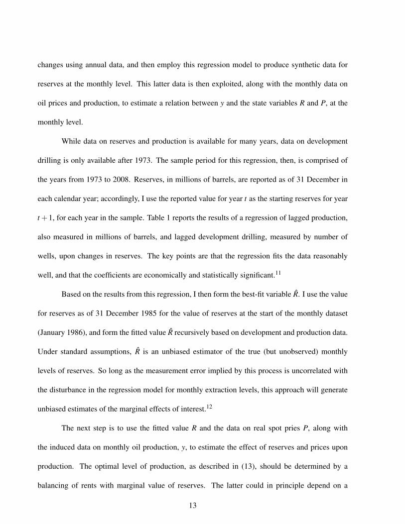
Based on the results from this regression, I then form the best-fit variable R. I use the value
for reserves as of 31 December 1985 for the value of reserves at the start of the monthly dataset
(January 1986), and form the fitted value R recursively based on development and production data.
Under standard assumptions, R is an unbiased estimator of the true (but unobserved) monthly
levels of reserves. So long as the measurement error implied by this process is uncorrelated with
the disturbance in the regression model for monthly extraction levels, this approach will generate
unbiased estimates of the marginal effects of interest.12
The next step is to use the fitted value R and the data on real spot pries P, along with
the induced data on monthly oil production, y, to estimate the effect of reserves and prices upon
production. The optimal level of production, as described in (13), should be determined by a
balancing of rents with marginal value of reserves. The latter could in principle depend on a
13
combination of prices or reserves. Marginal cost is inversely related to reserves, so the model
predicts that optimal output is proportional to the product of price and reserves, as well as the
product of reserves with marginal value. To this end, I regress linear and quadratic terms in R, as
well as interaction terms involving R and P, upon y; this regression model can be interpreted as a
Taylor’s series approximation of marginal value multiplied by R. In light of the time-series nature
of the data, I allow for serial correlation. To enhance comparability of observations from different
months, I convert production into millions of barrels per day. Table 2 presents results from the
regression analysis of extraction. The variables of interest are significant at or near the 5%-level or
better.
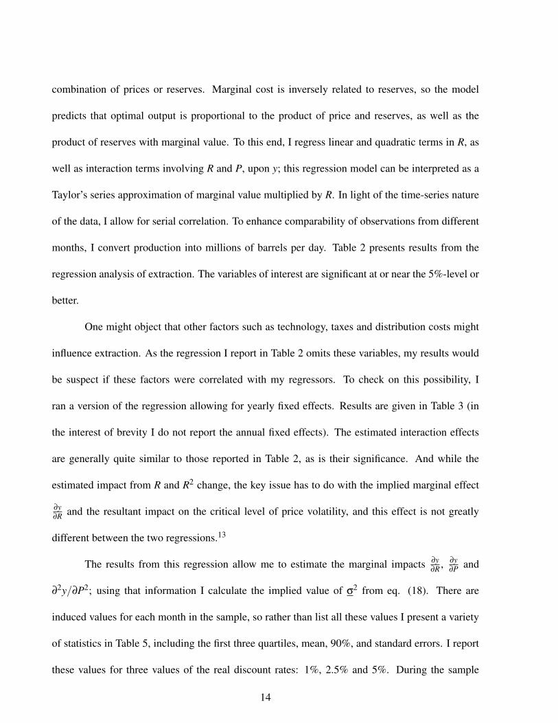
One might object that other factors such as technology, taxes and distribution costs might
influence extraction. As the regression I report in Table 2 omits these variables, my results would
be suspect if these factors were correlated with my regressors. To check on this possibility, I
ran a version of the regression allowing for yearly fixed effects. Results are given in Table 3 (in
the interest of brevity I do not report the annual fixed effects). The estimated interaction effects
are generally quite similar to those reported in Table 2, as is their significance. And while the
estimated impact from R and R2 change, the key issue has to do with the implied marginal effect
∂y∂R and the resultant impact on the critical level of price volatility, and this effect is not greatly
different between the two regressions.13
The results from this regression allow me to estimate the marginal impacts ∂y∂R , ∂y
∂P and
∂2y/∂P2; using that information I calculate the implied value of σ2 from eq. (18). There are
induced values for each month in the sample, so rather than list all these values I present a variety
of statistics in Table 5, including the first three quartiles, mean, 90%, and standard errors. I report
these values for three values of the real discount rates: 1%, 2.5% and 5%. During the sample
14
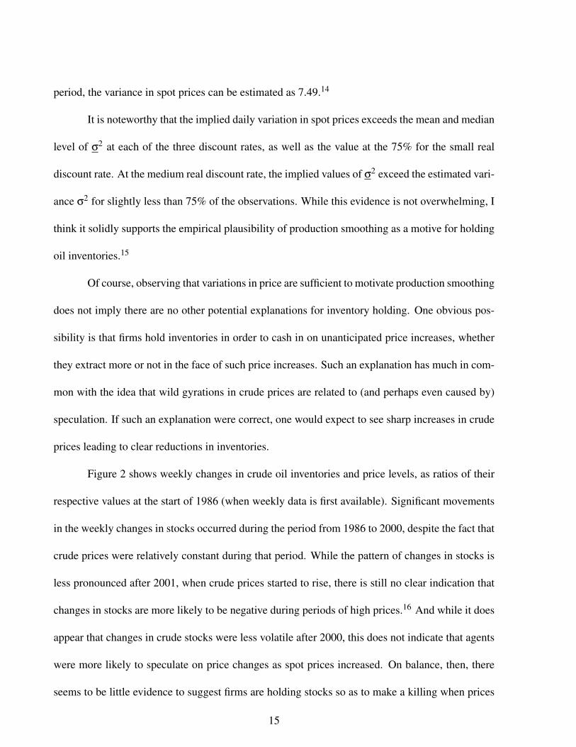
period, the variance in spot prices can be estimated as 7.49.14
It is noteworthy that the implied daily variation in spot prices exceeds the mean and median
level of σ2 at each of the three discount rates, as well as the value at the 75% for the small real
discount rate. At the medium real discount rate, the implied values of σ2 exceed the estimated vari-
ance σ2 for slightly less than 75% of the observations. While this evidence is not overwhelming, I
think it solidly supports the empirical plausibility of production smoothing as a motive for holding
oil inventories.15
Of course, observing that variations in price are sufficient to motivate production smoothing
does not imply there are no other potential explanations for inventory holding. One obvious pos-
sibility is that firms hold inventories in order to cash in on unanticipated price increases, whether
they extract more or not in the face of such price increases. Such an explanation has much in com-
mon with the idea that wild gyrations in crude prices are related to (and perhaps even caused by)
speculation. If such an explanation were correct, one would expect to see sharp increases in crude
prices leading to clear reductions in inventories.
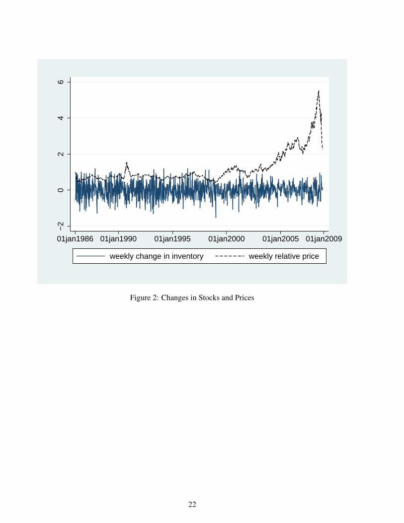
Figure 2 shows weekly changes in crude oil inventories and price levels, as ratios of their
respective values at the start of 1986 (when weekly data is first available). Significant movements
in the weekly changes in stocks occurred during the period from 1986 to 2000, despite the fact that
crude prices were relatively constant during that period. While the pattern of changes in stocks is
less pronounced after 2001, when crude prices started to rise, there is still no clear indication that
changes in stocks are more likely to be negative during periods of high prices.16 And while it does
appear that changes in crude stocks were less volatile after 2000, this does not indicate that agents
were more likely to speculate on price changes as spot prices increased. On balance, then, there
seems to be little evidence to suggest firms are holding stocks so as to make a killing when prices
15
rise dramatically.
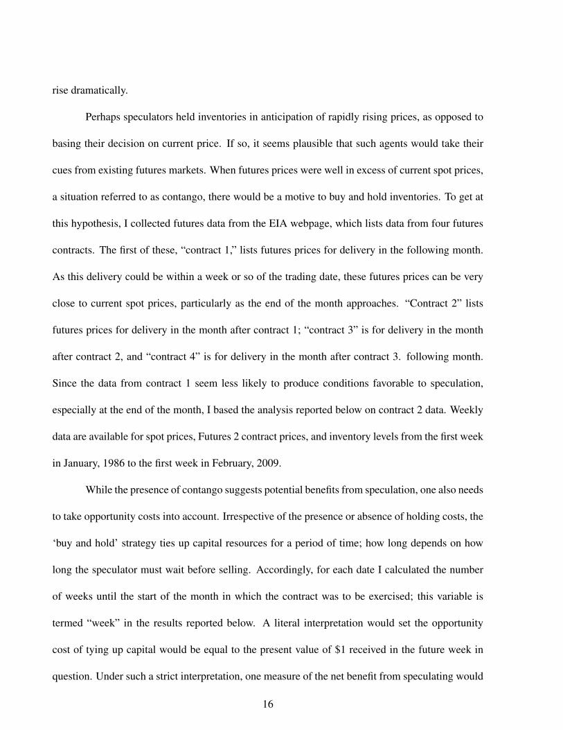
Perhaps speculators held inventories in anticipation of rapidly rising prices, as opposed to
basing their decision on current price. If so, it seems plausible that such agents would take their
cues from existing futures markets. When futures prices were well in excess of current spot prices,
a situation referred to as contango, there would be a motive to buy and hold inventories. To get at
this hypothesis, I collected futures data from the EIA webpage, which lists data from four futures
contracts. The first of these, “contract 1,” lists futures prices for delivery in the following month.
As this delivery could be within a week or so of the trading date, these futures prices can be very
close to current spot prices, particularly as the end of the month approaches. “Contract 2” lists
futures prices for delivery in the month after contract 1; “contract 3” is for delivery in the month
after contract 2, and “contract 4” is for delivery in the month after contract 3. following month.
Since the data from contract 1 seem less likely to produce conditions favorable to speculation,
especially at the end of the month, I based the analysis reported below on contract 2 data. Weekly
data are available for spot prices, Futures 2 contract prices, and inventory levels from the first week
in January, 1986 to the first week in February, 2009.
While the presence of contango suggests potential benefits from speculation, one also needs
to take opportunity costs into account. Irrespective of the presence or absence of holding costs, the
‘buy and hold’ strategy ties up capital resources for a period of time; how long depends on how
long the speculator must wait before selling. Accordingly, for each date I calculated the number
of weeks until the start of the month in which the contract was to be exercised; this variable is
termed “week” in the results reported below. A literal interpretation would set the opportunity
cost of tying up capital would be equal to the present value of $1 received in the future week in
question. Under such a strict interpretation, one measure of the net benefit from speculating would
16
be ln(Pt,T ) = T ln(pt), where Pt,T is the price of a future contract at time t for delivery in T periods
and pt is the spot price in period t. Under this interpretation, a regression of changes in inventories
upon the regressors ln(Pt,T ),T ln(pt), and T would yield coefficients k1,k2 and k3, with k1 positive
and the other two negative; it would also explain much of the variation in stock changes. (A literal
interpretation of the coefficients would be k2 =−(1+ r)and k3 = c, where r is the market interest
rate and c is the unit cost of holding inventory for a week). A less strict interpretation would regress
changes in inventories upon the regressors ln(Pt,T /pt) and T , where presumably the coefficient
on the former would be positive (reflecting the sensitivity of stockpiling decisions to potential
gains) and the coefficient on T would be negative, reflecting the opportunity cost of tying up
capital while stockpiling. Alternatively, one might replace the log-ratio of futures to spot price with
the difference between future and spot price; the coefficients would take similar interpretations.
In the results reported below, I refer to these regressions as ‘Regression 1,’ ‘Regression 2’ and
‘Regression 3,’ respectively.
The results from these three regressions are collected into Table 5. Column 2-4 report re-
sults from, respectively, Regressions 1, 2 and 3; standard errors are listed in parentheses below the
corresponding point estimates. One is struck by the poor performance of each regression. Indeed,
the only variable that exerts a statistically significant effect is the difference between future and
spot price, as reported in Regression 3; even here the significance is only at the 10% level. None
of the three regressions explain any meaningful amount of the variation is inventory adjustments.
Overall, these results indicate that speculation had little to do with inventory accumulation during
the sample period.
17
5 Conclusion
In this paper, I present a model of firm behavior when oil prices are stochastic. In this frame-
work, the firm has an incentive to hold inventories if prices are sufficiently volatile. Using data on
monthly crude prices and privately-held U.S. inventories, I find evidence that there was sufficient
volatility in crude prices over the period from early 1986 to late 2008 to motivate inventory hold-
ing. By contrast, the evidence that firms held inventories to speculate on price movements does
not seem very strong. I believe the conclusion is that inventories are more likely to be motivated
by attempts to smooth marginal production costs than by speculative motives.
My model assumes that the entire cost of production is born at the deposit. In particular,
extracted oil can instantly and costlessly be delivered to market, and storage of inventories is
costless. These assumptions may be legitimately questioned as unrealistic. Shipping costs for
crude oil can be a significant share of delivered price, and there is often an important lag between
extraction and sale. However, my central findings seem likely to be robust to each of these potential
extensions.
Adding distribution costs to the model above has no major effects upon my central results.
While such an alteration lowers the expected gains from holding inventories, it has an equivalent
effect on current profits. Correspondingly, the key comparison is between the capitalized value
of “distribution rents” (price less marginal distribution cost) and the expected rate of change in
distribution rents. If the unit cost of distribution is taken as constant, then my model may be
applied by interpreting price as distribution rent. This suggests smaller initial sales (and higher
initial price) in conjunction with slower growth of prices over time. Such an alteration reduces the
value of inventories, but not the finding that sufficient variation in prices will induce firms to hold
18
stockpiles.
Adding storage costs to the model also leaves the central result unchanged. While the
presence of storage costs would make it less desirable to hold inventories, there can still be a
motive with sufficiently variable demand. The results in Table 4 suggest that demand is often
considerably more variable than required to motivate the holding of inventories. Thus, it seems
plausible that the results reported above are robust to storage costs.
It seems most plausible that there is a lag between extraction and sales, as crude oil must be
refined prior to delivery of the final good. An extension of the analysis to allow for such lags can
be constructed by distinguishing between the date of sales and the date of extraction. Abel (1985)
showed that competitive firms would generally have an incentive to hold inventories in the context
of lags between production and sales, to facilitate speculation. His results would seem applicable
here as well. Indeed, Blanchard and Fisher (1989) suggest that this motive may be at least as
important as the production smoothing motive in explaining inventories of most commodities.
19
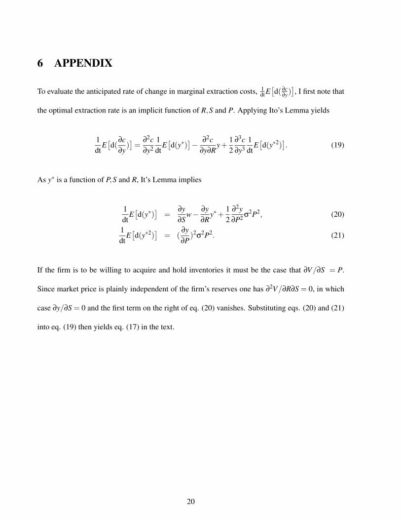
6 APPENDIX
To evaluate the anticipated rate of change in marginal extraction costs, 1dtE
[d(∂c
∂y)], I first note that
the optimal extraction rate is an implicit function of R,S and P. Applying Ito’s Lemma yields
1dt
E[d(
∂c∂y
)]=
∂2c∂y2
1dt
E[d(y∗)
]− ∂2c∂y∂R
y+12
∂3c∂y3
1dt
E[d(y∗2)
]. (19)
As y∗ is a function of P,S and R, It’s Lemma implies
1dt
E[d(y∗)
]=
∂y∂S
w− ∂y∂R
y∗+12
∂2y∂P2 σ2P2, (20)
1dt
E[d(y∗2)
]= (
∂y∂P
)2σ2P2. (21)
If the firm is to be willing to acquire and hold inventories it must be the case that ∂V/∂S = P.
Since market price is plainly independent of the firm’s reserves one has ∂2V/∂R∂S = 0, in which
case ∂y/∂S = 0 and the first term on the right of eq. (20) vanishes. Substituting eqs. (20) and (21)
into eq. (19) then yields eq. (17) in the text.
20
2000
0030
0000
4000
00m
onth
ly in
vent
orie
s, 1
000
bbls
1920jan 1930jan 1940jan 1950jan 1960jan 1970jan 1980jan 1990jan 2000jan 2010janmonth
Figure 1: U.S. Petroleum Stocks
21
−2
02
46
01jan1986 01jan1990 01jan1995 01jan2000 01jan2005 01jan2009
weekly change in inventory weekly relative price
Figure 2: Changes in Stocks and Prices
22
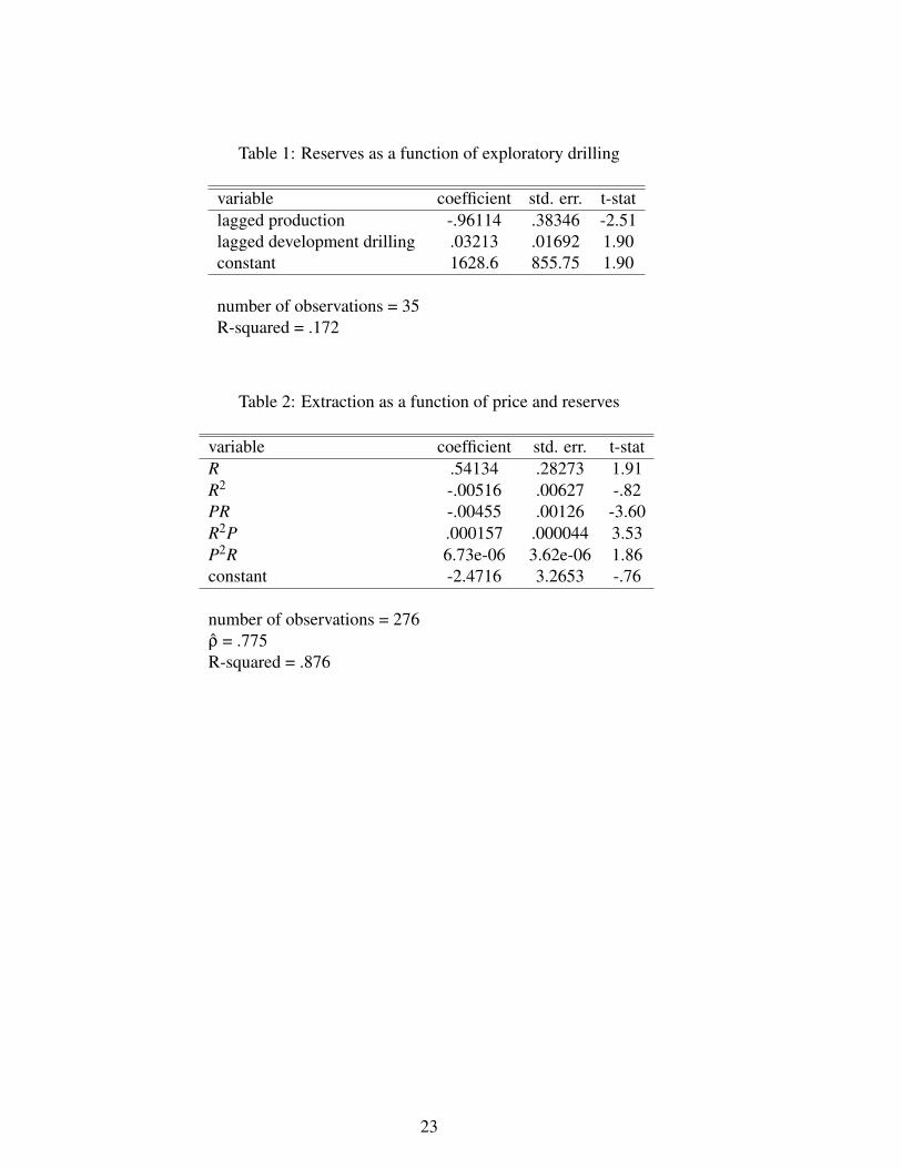
Table 1: Reserves as a function of exploratory drilling
variable coefficient std. err. t-statlagged production -.96114 .38346 -2.51lagged development drilling .03213 .01692 1.90constant 1628.6 855.75 1.90
number of observations = 35R-squared = .172
Table 2: Extraction as a function of price and reserves
variable coefficient std. err. t-statR .54134 .28273 1.91R2 -.00516 .00627 -.82PR -.00455 .00126 -3.60R2P .000157 .000044 3.53P2R 6.73e-06 3.62e-06 1.86constant -2.4716 3.2653 -.76
number of observations = 276ρ = .775R-squared = .876
23
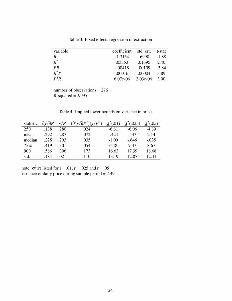
Table 3: Fixed effects regression of extraction
variable coefficient std. err. t-statR -1.3154 .6998 -1.88R2 .03353 .01395 2.40PR -.00418 .00109 -3.84R2P .00016 .00004 3.89P2R 6.07e-06 2.03e-06 3.00
number of observations = 276R-squared = .9995
Table 4: Implied lower bounds on variance in price
statistic ∂y/∂R y/R (∂2y/∂P2)(y/P2) σ2(.01) σ2(.025) σ2(.05)25% .138 .280 .024 -6.81 -6.06 -4.89mean .292 .287 .072 -.424 .537 2.14median .225 .293 .035 -1.09 -.646 -.03575% .419 .301 .054 6.48 7.37 8.6790% .586 .306 .173 16.62 17.39 18.68s.d. .184 .021 .110 13.19 12.87 12.41
note: σ2(r) listed for r = .01, r = .025 and r = .05variance of daily price during sample period = 7.49
24
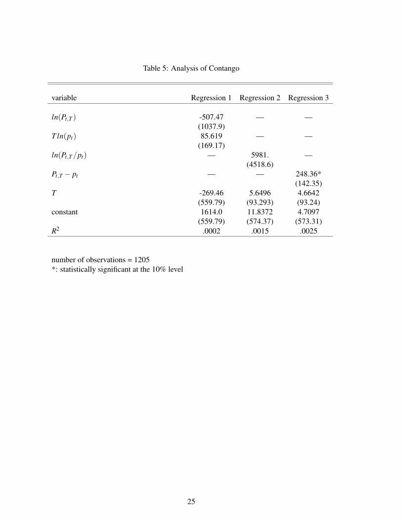
Table 5: Analysis of Contango
variable Regression 1 Regression 2 Regression 3
ln(Pt,T ) -507.47 — —(1037.9)
T ln(pt) 85.619 — —(169.17)
ln(Pt,T /pt) — 5981. —(4518.6)
Pt,T − pt — — 248.36*(142.35)
T -269.46 5.6496 4.6642(559.79) (93.293) (93.24)
constant 1614.0 11.8372 4.7097(559.79) (574.37) (573.31)
R2 .0002 .0015 .0025
number of observations = 1205*: statistically significant at the 10% level
25
References
Abel, A. (1985). Inventories, stockouts, and production smoothing, Review of Economic Studies
52: 283–194.
Adelman, M. A. (1995). Genie Out of the Bottle: World Oil Since 1970, MIT Press, Cambridge,
MA.
Arrow, K. J., Karlin, S. and Scarf, H. (1958). Studies in the mathematical theory of inventory and
production, Stanford University Press, Palo Alto CA.
Blanchard, O. J. and Fisher, S. (1989). Lectures on Macroeconomics, MIT Press, Cambridge, MA.
Brennan, M. J. and Schwartz, E. J. (1985). Evaluating natural resource investments, Journal of
Business 58: 135–158.
Chow, G. C. and Lin, A.-l. (1971). Best linear unbiased interpolation, distribution, and extrapola-
tion of time series by related series, The Review of Economics and Statistics 53: 372–375.
Dixit, A. and Pindyck, R. (1993). Investment under uncertainty, Princeton University Press, Prince-
ton, NJ.
Kamien, M. and Schwartz, N. (1991). Dynamic Optimization: The Calculus of Variations and
Optimal Control in Economics and Management, North Holland, Amsterdam.
Mason, C. F. (2001). Nonrenewable resources with switching costs, Journal of Environmental
Economics and Management 42: 65–81.
Pindyck, R. S. (1980). Uncertainty and exhaustible resource markets, Journal of Political Economy
88: 1203–1225.
26
Pindyck, R. S. (1982). Uncertainty and the behavior of the firm, American Economic Review
72: 415–427.
Santos-Silva, J. and Cardoso, F. N. (2001). The chow-lin method using dynamic models, Economic
Modelling 18: 262–280.
Slade, M. (1988). Grade selection under uncertainty: least cost last and other anomalies, Journal
of Environmental Economics and Management 15: 189–205.
27
Notes
1 A third explanation is that inventories might be held to insure against running out of the key
resource (the so-called ”stock-out” motive). It is hard to believe this motive played a major role in
the U.S. oil industry, however: average daily input into U.S. refiners during the same period was
just over 14 million barrels per day, and never exceeded 16.5 million barrels per day. As such, the
stockpile of crude oil would have supplied all U.S. refiners for almost 20 days.
2 If Pt < µt the firm would be inclined to sell all extracted oil along with any accumulated
inventories. If any inventories were held the firms sales rate would then be infinite, which as I note
in the text would violate market clearing. But if the firm has never acquired any inventories there is
nothing to prevent Pt < µt . In fact, this is the most likely outcome in the deterministic framework.
3 While I assume geometric Brownian motion for analytic convenience, a number of previous
authors have made similar assumptions (Brennan and Schwartz, 1985; Dixit and Pindyck, 1993;
Mason, 2001; Pindyck, 1980; Slade, 1988).
4 See Brennan and Schwartz (1985), Dixit and Pindyck (1993) and Mason (2001) for analysis
of such a model.
5 Shadow values smaller than current price would induce the firm to discontinuously reduce
its inventory stock, which would imply selling at an infinite rate. As discussed above, this cannot
occur because of market clearing.
6 As rents rise at the rate of interest, while price generally rises less rapidly, it follows that
28
marginal costs must also rise at less than the rate of interest.
7 For example, in December of 2008 Royal Dutch - Shell PLC anchored a supertanker full of
crude oil off the British coast in anticipation of higher prices for future delivery.
8 With these assumptions ∂3c/∂y3 = 0. As ∂3c/∂y3 exerts a positive influence on the expres-
sion in eq. (17), one can argue that this assumption generates the least compelling case for holding
inventories.
9 As marginal costs are linear, results at aggregate level map naturally into results at the level
of the individual field-reservoir. If one is willing to draw an analogy between individual field-
reservoirs and firms these results are directly relevant to the model discussed in section 3 above.
10 In fact, spot prices are reported on a daily, weekly, monthly and annual basis. Data on stock-
piles are available including or excluding the U. S. strategic petroleum reserve (SPR). As the SPR
is both publicly held, and hence motivated by political – as opposed to economic considerations –
it seems clear that the data excluding the SPR is preferable for my purposes.
11 The coefficient on lagged production is very close to -1, as expected. The coefficient on
development drilling, while only significant only at the 7% level, is of the correct sign.
12 However, the approach will impact the standard errors. The results reported below are based
on robust standard errors, and so correct for this possibility. An alternative approach to the one I
use here is to estimate a relation between extraction and prices and reserves using annual data.
The disadvantage of using annual data is the corresponding reduction in number of observations.
A regression using annual data generates similar results to those reported in Table 2, in the sense
29
that estimated coefficients have the same signs and are generally the same order of magnitude.
However, because production data are only available since 1986, only 22 annual observations are
available. With such a small data set there are very few degrees of freedom, and none of the
coefficients are statistically significant.
13 Specifically, for both variants of the regression over half the observations yield induced
levels of the critical variance which are smaller than 7.49; for values of the real discount rate less
than 5% over three-quarters of the observations fall below 7.49.
14 The variance of monthly real spot price during the sample period is .2498. Assuming
that prices evolve according to geometric Brownian motion implies that prices are log-normally
distributed. During the sample period, the mean and variance of real spot prices are 34.9842
and 347.24, respectively. The formulae for mean and variance of a log-normal are em+s2/2 and
e2[m+s2]−e2m+s2, where m and s2 are mean and variance of the underlying normal random variable,
here the percentage monthly change in real price. Based on this information, it is straightforward
to derive .2498 as an estimate of the variance for a typical month. Multiplying by N, the number
of daily observations that would have led to that value, gives an estimate of the daily variance —
the value that most closely captures the spirit of the problem at hand. Thus, I derive σ2 = 7.49.
15 As indicated in eq. (10), firms could be motivated to hold inventories even in the absence of
stochastic demand so long as the percentage change in production and the ration of production to
reserves matched up just right. To investigate this possibility, I formed the discrete time approxi-
mation to percentage change in production, ∆yt/yt = (yt+1−yt)/yt and the ration of production to
reserves, yt/Rt , for each month t in the sample period. Assuming η = 2, the construct ∆/y+ y/2R
30
would equal the interest rate. For the sample period, the average value of this construct is 4.2273,
implying an interest rate of over 422%. Alternatively, one could run a linear regression of ∆y/y
on y/2R; such a regression should yield an intercept of r/η− 1 and a slope coefficient of −1/η.
Performing such a regression yields estimated coefficients -.0742 for r/η−1 and .00822 for−1/η.
Plainly, these results do not lend much support to the notion that firms would have been motivated
to hold inventories absent stochastic demand.
16 In fact, the average change in stocks was negative prior to 2000 (-216,726.2 barrels) and
positive after (179,228.6 barrels). This difference in average values, while intriguing, is not sta-
tistically significant: the corresponding standard deviations were two orders of magnitude larger.
Thus, there is no evidence of significantly smaller values for changes in stocks as prices increased.
A similar patter emerges if one compares levels of inventories against price. During the sample
period there are dramatic swings in price, from below 50% of the initial level to over 550% of the
initial level. But even with these dramatic swings in price crude stock levels are always within
20% of the initial value. More to the point, there seems to be little evidence that stocks are drawn
down during times of particularly large prices, nor are stocks built up during periods of low prices.
31