This paper presents preliminary findings and is being distributed to economists

and other interested readers solely to stimulate discussion and elicit comments.

The views expressed in this paper are those of the authors and do not necessarily

reflect the position of the Federal Reserve Bank of New York or the Federal

Reserve System. Any errors or omissions are the responsibility of the authors.

Federal Reserve Bank of New York

Staff Reports

Why Do Banks Target ROE?

George Pennacchi

João A. C. Santos

Staff Report No. 855

June 2018

Why Do Banks Target ROE?

George Pennacchi and João A. C. Santos

Federal Reserve Bank of New York Staff Reports, no. 855

June 2018

JEL classification: G21, G28

Abstract

Historically, nonfinancial corporations relied on performance targets linked to their EPS. Up until

the 1970s, banks also appeared to follow a similar practice, but since then they have favored

ROE. Equity investors seem to be aware of these differences because EPS growth is better at

explaining nonfinancials’ stock market value while ROE is better at explaining banks’ market

values. In this paper we present a model of a bank with fixed-rate deposit insurance that faces

increasing competition that erodes its charter value. When under these conditions the bank

chooses its capital to maximize shareholder value, its performance based on ROE is much better

than its performance based on EPS. We argue that such a situation characterized the banking

industry during the 1970s and explains why it adopted an ROE target.

Key words: banks, ROE, EPS

_________________

Santos: Federal Reserve Bank of New York, Nova School of Business and Economics (email: joao.santos@ny.frb.org). Pennacchi: University of Illinois (email: gpennacc@illinois.edu). The authors thank Kate Bradley and Sooji Kim for their outstanding research assistance. The views expressed in this paper are those of the authors and do not necessarily reflect the position of the Federal Reserve Bank of New York or the Federal Reserve System. To view the authors’ disclosure statements, visit https://www.newyorkfed.org/research/staff_reports/sr855.html.

1

1. Introduction

This paper considers the question of why banks emphasize Return on Equity (ROE) as a performance

metric while non-financial firms tend to measure their performance based on Earnings per Share (EPS). Our

explanation for this difference hinges on two particular features of the banking industry. First, starting in the

1970s, the banking industry was subject to increasing competition from nonbank financial institutions, such

as money market mutual funds. Greater competition also resulted from a liberalization of intra-state and

inter-state bank branching restrictions during the 1980s and 1990s. Second, banks benefited from deposit

insurance that we argue was not fairly priced. We show that these two rather special factors pertaining to

banks provide a rationale for why they would chose to emphasize ROE rather than EPS.

We first document from banks’ annual reports that they started to discuss ROE only in the late 1970s.

Prior to that time, banks tended to focus on performance metrics that were similar to those of nonfinancial

firms. We also show that banks’ special emphasis on ROE appears to be important. ROE is the most

common accounting metric for the compensation contracts of bank managers, while EPS is the most

common standard for the compensation of nonfinancial firm executives. In addition, stock market investors

appear to differentiate between banks and nonfinancial firms. The market-to-book values of banks’ stocks

react more to ROE announcements than EPS announcements while the reverse occurs for non-financial

firms.

Prior work has noted that banks focus on ROE but it is a flawed performance target because it does not

account for the risk of equity.1 Haldane and Alessandri (2009) show that for UK banks, “the 1970s signaled a

sea-change” as banks’ average ROE jumped from around 7% to around 20%. They attribute it to lower

capital and greater bank asset risk. Perhaps closes to out paper is Begenau and Stafford (2016). They show

empirically that banks with low Return on Assets (ROA) attempt to maintain a high ROE by using higher

leverage. Moreover, stock market-to-book value measures of bank equity are highly correlated with ROE.

Putting these two facts together, they suggest that banks manipulate ROE upwards via leverage because

stock market investors (inefficiently) focus on ROE.

Our paper departs from Begenau and Stafford (2016) in an important way. We do not assume that

banks’ choose leverage specifically to manipulate ROE because investors’ irrationally target ROE. Rather,

1 For example, see Admati, DeMarzo, Hellwig, and Pfleider (2013).

2

we present a structural model of a bank that rationally maximizes its shareholders’ value in excess of the

shareholders’ contributed capital. The model has several key ingredients. First, the bank’s deposits are

insured by the government. Second, the bank has “charter” or “franchise” value that derives from its ability

to pay interest on insured deposits that is below a competitive risk-free rate. Third, the bank must pay

corporate income taxes.

We then use this model to consider the excess shareholder value-maximizing response of the bank

when it faces increasing competition that lowers the spread between a competitive risk-free rate and its

insured deposit interest rate. In other words, we analyze a bank’s reaction to an erosion of its charter value.

The model shows that the bank reduces its choice of initial capital, and this reduction is greater in magnitude

when the bank is subject to fixed-rate deposit insurance compared to when it is subject to fairly-priced

deposit insurance. We then ask what are the consequences for EPS growth and ROE growth when a bank

makes this excess shareholder value-maximizing reduction in capital.

If a bank did not adjust its capital, EPS growth would be negative but small in magnitude due to the

mechanical effect from greater competition that decreases the bank’s deposit spread and reduces its net

interest margin. However, when the bank rationally reduces its capital, EPS growth worsens further.

Moreover, the magnitude of the decline in EPS growth is greater when the bank is subject to fixed-rate

deposit insurance compared to fairly-priced deposit insurance.

Regarding ROE growth, we also show that if a bank did not adjust its capital, ROE growth would be

negative though slightly smaller in magnitude compared to EPS growth. Interestingly, however, when a bank

rationally reduces its initial capital in response to greater competition, the consequence for ROE growth is

exactly the opposite to that of EPS growth. Specifically, the bank’s rational reduction in capital causes a rise

in ROE growth that can easily offset the mechanical decline from a lower net interest margin. Moreover, the

resulting rise in ROE growth is greater when the bank has fixed-rate deposit insurance compared to fairly-

priced deposit insurance.

Note that our model implies there would be no tendency for ROE growth to be greater than EPS

growth for a firm whose charter value was not declining and that did not enjoy a government guarantee of its

debt. Taken together, these model results provide an explanation for why banks would particularly prefer

ROE growth to EPS growth as their performance metric. Their preference is not due to any strategic

3

manipulation of ROE per se. Rather, it is because ROE simply makes banks look better when then they

rationally respond to greater competition.

Of course, the credibility of these model results depends on the realism of our model’s assumptions.

Following the presentation of our model, we provide evidence that starting in the 1970s, U.S. banks were

indeed exposed to increasing competition from nonbank financial institutions (a.k.a. “shadow” banks).

Competition in the banking sector further intensified in the 1980s following states’ decisions to lift

restrictions on branching within their borders and to permit out-of-state institutions to acquire their banks.

With respect to the FDIC deposit insurance premiums, historically they have been assessed without regard to

individual banks’ risk. It was only in 1991 that the FDIC changed the flat-rate assessment system to one

based on the bank’s risk. Conceptually this was a significant departure from the historic flat-rate practice, but

effective insurance premiums charged to banks in the following years remained only mildly linked to bank

risk.

The paper proceeds as follows. Section 2 reviews the performance targets that banks and nonfinancials

have use in their annual reports over time. Section 3 investigates whether the stock market responds to firms’

choice of a performance target. Section 4 presents a formal model to explain why banks would prefer ROE to

EPS as a performance measure. Section 5 presents evidence consistent with our model’s assumptions.

Section 6 concludes.

2. Banks’ and Nonfinancial Firms’ Performance Targets over Time

Historically, nonfinancial corporations have emphasized performance metrics/targets that are linked to their

earnings per share (EPS) in their communications with shareholders. Banks also appear to have favored

metrics linked to EPS up until the late 1970s, but since then their preferences have shifted towards ROE.

These differences are apparent in the annual reports of four firms, one nonfinancial (Black & Decker

Manufacturing) and three banks (Bank of Boston Corporation, Chemical New York Corporation and

JPMorgan Chase) that we were able to access going as far back as the 1940s.2

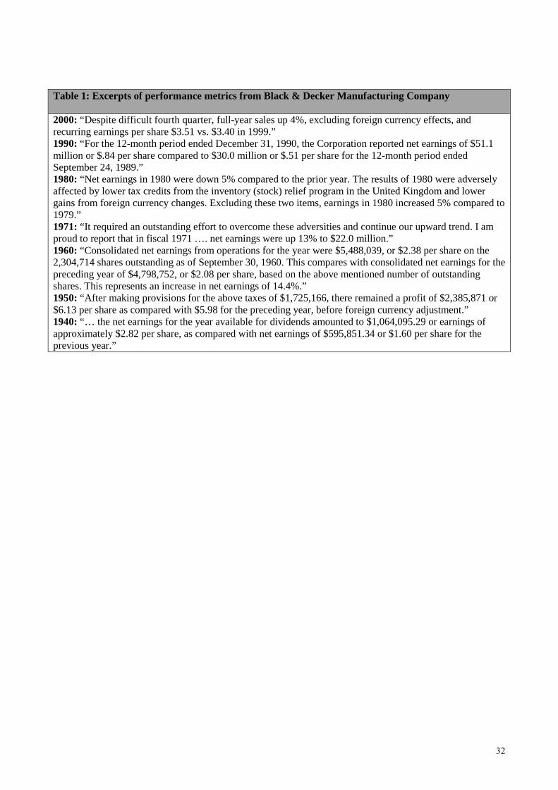
As we can see from Table 1, which contains excerpts from Black & Decker Manufacturing

corporation annual reports going back to 1940, there is no reference to ROE. Instead, every year the report

2 Chemical bank merged with Chase Manhattan bank in 1995, which in turn acquired JPMorgan in 2000.

4

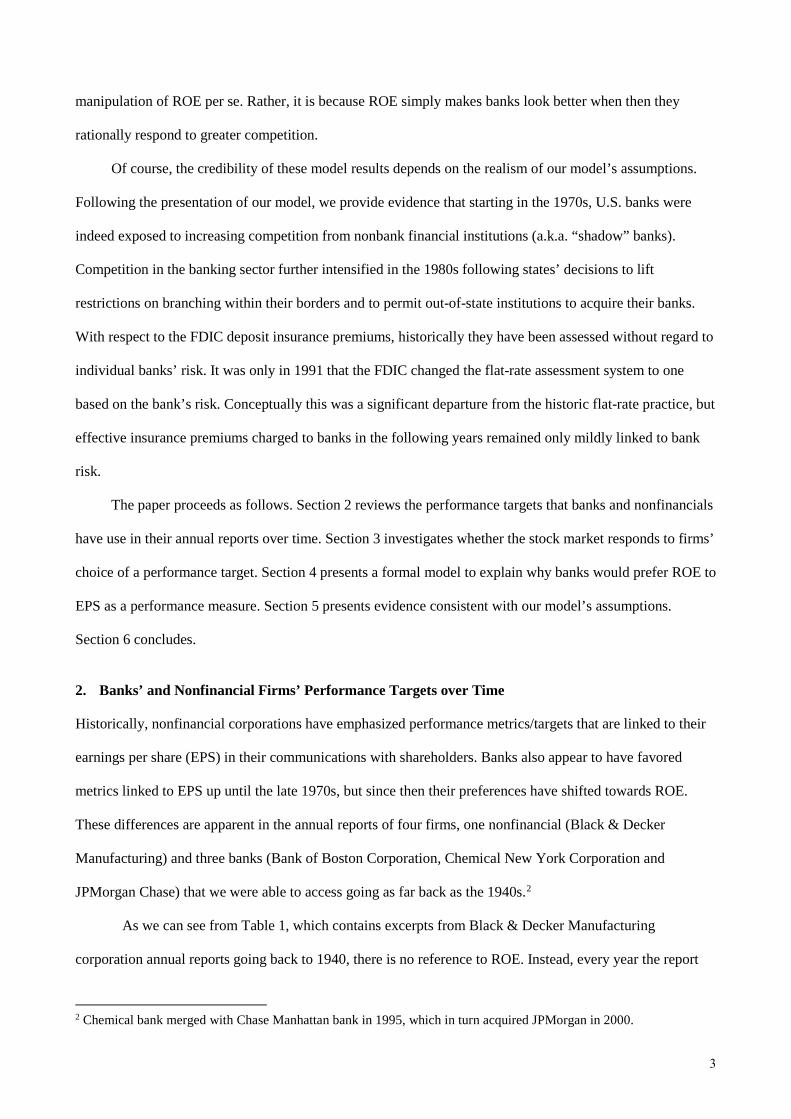
highlights the company’s EPS. For example, in its 1940 annual report Black & Decker noted that “… the net

earnings for the year available for dividends amounted to $1,064,095.29 or earnings of approximately $2.82

per share, as compared with net earnings of $595,851.34 or $1.60 per share for the previous year.” By 2000,

the company was still using a remarkably similar language in its communication with shareholders “Despite

difficult fourth quarter, full-year sales up 4%, excluding foreign currency effects, and recurring earnings per

share $3.51 vs. $3.40 in 1999.”

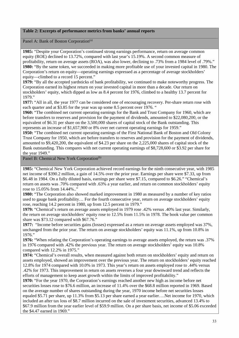
Looking at Table 2, which reports excerpts from the annual reports of three of the largest US banks

(and their predecessors): Bank of Boston Corporation (Panel A), Chemical New York Corporation (Panel B),

and JPMorgan Chase (Panel C), we see that up until the late 1970s these banks, like nonfinancial

corporations, use to highlight EPS, making only sporadic references to ROE. However, since then they

started to use ROE when communicating their performance to shareholders.

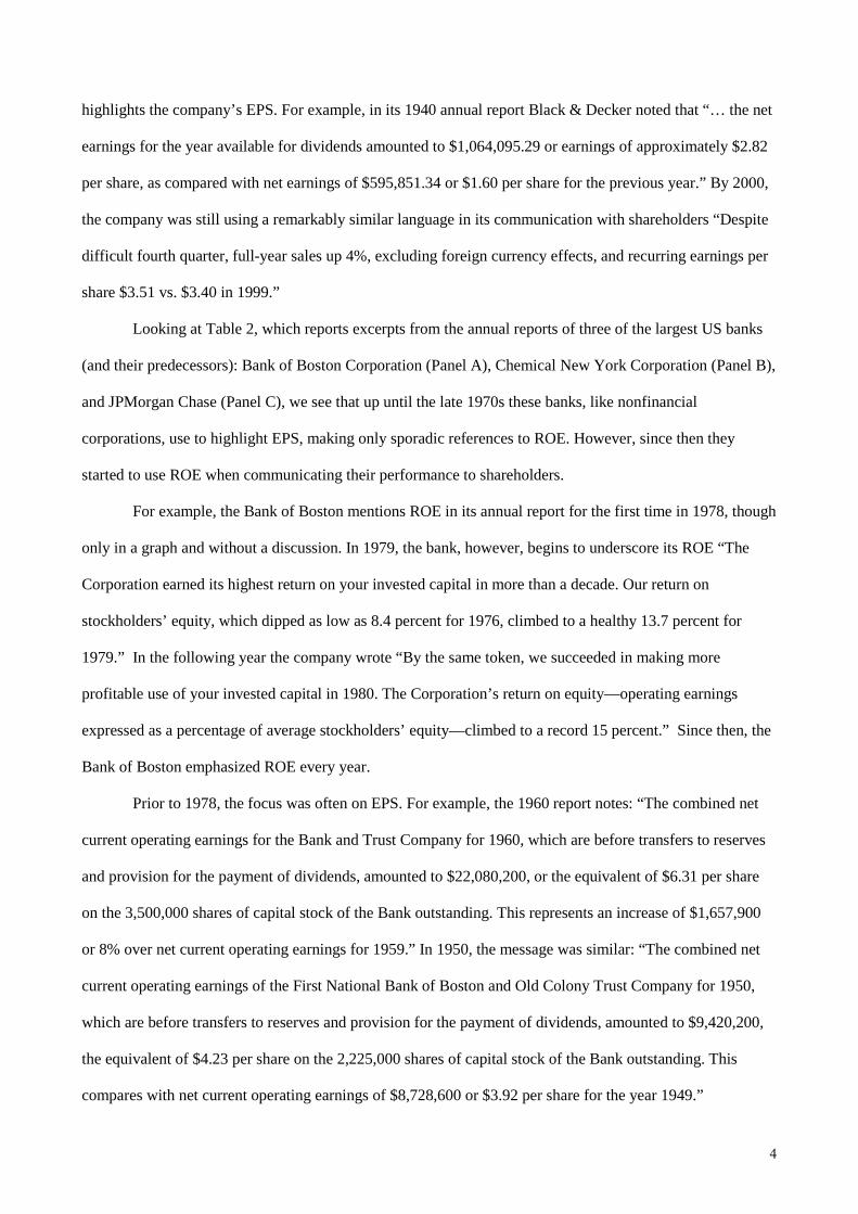
For example, the Bank of Boston mentions ROE in its annual report for the first time in 1978, though

only in a graph and without a discussion. In 1979, the bank, however, begins to underscore its ROE “The

Corporation earned its highest return on your invested capital in more than a decade. Our return on

stockholders’ equity, which dipped as low as 8.4 percent for 1976, climbed to a healthy 13.7 percent for

1979.” In the following year the company wrote “By the same token, we succeeded in making more

profitable use of your invested capital in 1980. The Corporation’s return on equity—operating earnings

expressed as a percentage of average stockholders’ equity—climbed to a record 15 percent.” Since then, the

Bank of Boston emphasized ROE every year.

Prior to 1978, the focus was often on EPS. For example, the 1960 report notes: “The combined net

current operating earnings for the Bank and Trust Company for 1960, which are before transfers to reserves

and provision for the payment of dividends, amounted to $22,080,200, or the equivalent of $6.31 per share

on the 3,500,000 shares of capital stock of the Bank outstanding. This represents an increase of $1,657,900

or 8% over net current operating earnings for 1959.” In 1950, the message was similar: “The combined net

current operating earnings of the First National Bank of Boston and Old Colony Trust Company for 1950,

which are before transfers to reserves and provision for the payment of dividends, amounted to $9,420,200,

the equivalent of $4.23 per share on the 2,225,000 shares of capital stock of the Bank outstanding. This

compares with net current operating earnings of $8,728,600 or $3.92 per share for the year 1949.”

5

The Chemical New York Corporation follows a pattern similar to the Bank of Boston’s. It highlights

ROE for the first time in in its 1980 annual report: “The Corporation also showed marked improvement in

1980 as measured by a number of key ratios used to gauge bank profitability… For the fourth consecutive

year, return on average stockholders’ equity rose, reaching 14.2 percent in 1980, up from 12.5 percent in

1979.” In the second half of the 1970s, the company mentions ROE in its annual report only very briefly and

often towards the end of it. For example, in 1977 it writes “Income before securities gains (losses) expressed

as a return on average assets employed was 37%, unchanged from the prior year. The return on average

stockholders’ equity was 11.1%, up from 10.8% in 1976.” The very first year that we found a reference to

ROE was 1974 near the back of the annual report: “Chemical’s overall results, when measured against both

return on stockholders’ equity and return on assets employed, showed an improvement over the previous

year. The return on stockholders’ equity reached 12.8% for 1974 compared with 10.0% in 1973. This year’s

return on assets employed rose to .44% versus .42% for 1973.”

Prior to those years, Chemical often emphasized EPS. For example, the annual report for 1960 notes:

“Net operating earnings before taxes amounted to $74,446,000, an increase of $6,371,000 over 1959. Net

operating earnings after taxes totaled $40,907,000, a 5% gain over our 1959 earnings of $38,978,000. Net

per share was $4.83 for 1960 against $4.60 for 1959.” Similarly, the report for 1950 notes: “Net operating

income for 1950 amounted to $4,301,687, the equivalent of $7.17 per share on the 600,000 shares of capital

stock of the Company, as compared with $3,925,613 or $6.54 per share in 1949.”

JPMorgan Chase also follows a somewhat similar pattern. Starting in the late 1970s there is a

growing focus on ROE. For example, Chase Manhattan writes in its 1979 report: “Our return on average

assets has improved steadily over the past several years and in 1979 reached .52%, up from .36% in 1978.

Increased earnings in 1979 also resulted in an improvement in the return on average common stockholders’

equity which advanced from 10.3% in 1978 to 15.3% in 1979.” The 1980 report notes “Increased earnings

have also resulted in an improvement in the return on average common stockholders’ equity to 15.8% in

1980 from 15.3% in 1979 and 10.3% in 1978” and by 2000, JPMorgan Chase report notes “The growth

potential that we see at JPMorgan Chase is reflected in the performance targets that we have outlined as

long-term goals: Average cash return on equity of 20%-25%. Cash earnings per share growth of 15%.

Certainly, we did not achieve these financial targets in 2000. Revenue growth was affected by challenging

6

markets, and our cash return on equity fell to 18%.”

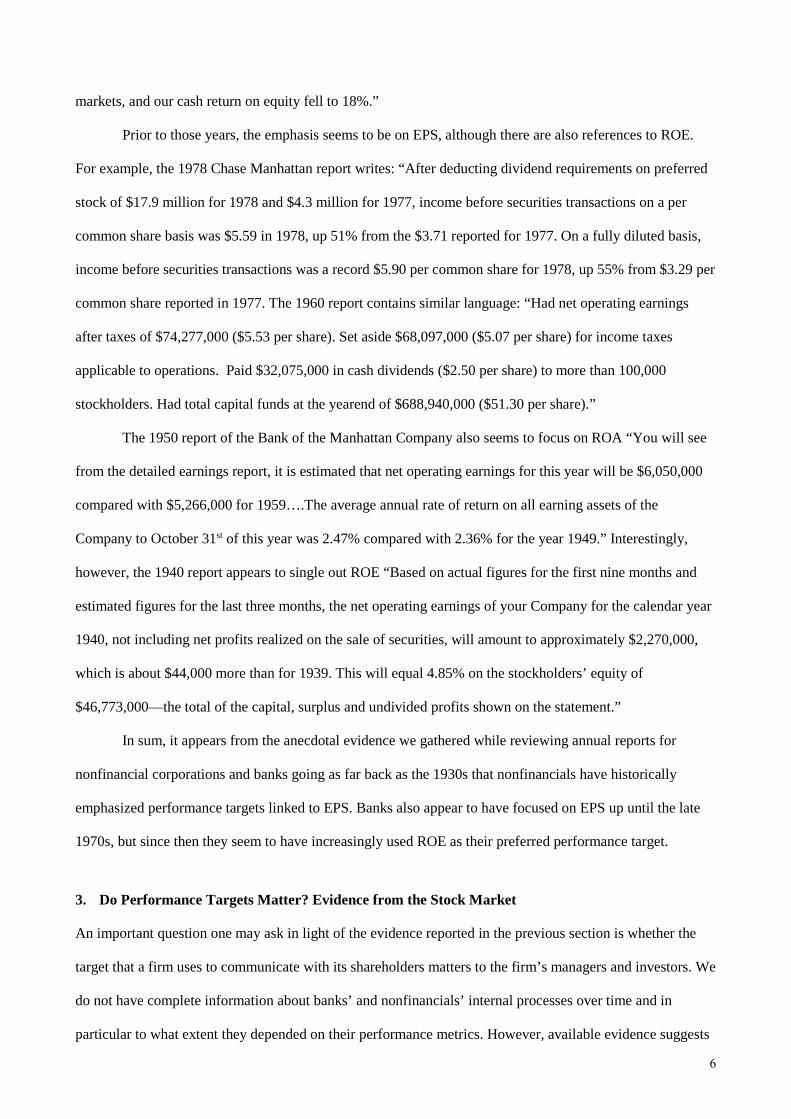
Prior to those years, the emphasis seems to be on EPS, although there are also references to ROE.

For example, the 1978 Chase Manhattan report writes: “After deducting dividend requirements on preferred

stock of $17.9 million for 1978 and $4.3 million for 1977, income before securities transactions on a per

common share basis was $5.59 in 1978, up 51% from the $3.71 reported for 1977. On a fully diluted basis,

income before securities transactions was a record $5.90 per common share for 1978, up 55% from $3.29 per

common share reported in 1977. The 1960 report contains similar language: “Had net operating earnings

after taxes of $74,277,000 ($5.53 per share). Set aside $68,097,000 ($5.07 per share) for income taxes

applicable to operations. Paid $32,075,000 in cash dividends ($2.50 per share) to more than 100,000

stockholders. Had total capital funds at the yearend of $688,940,000 ($51.30 per share).”

The 1950 report of the Bank of the Manhattan Company also seems to focus on ROA “You will see

from the detailed earnings report, it is estimated that net operating earnings for this year will be $6,050,000

compared with $5,266,000 for 1959….The average annual rate of return on all earning assets of the

Company to October 31st of this year was 2.47% compared with 2.36% for the year 1949.” Interestingly,

however, the 1940 report appears to single out ROE “Based on actual figures for the first nine months and

estimated figures for the last three months, the net operating earnings of your Company for the calendar year

1940, not including net profits realized on the sale of securities, will amount to approximately $2,270,000,

which is about $44,000 more than for 1939. This will equal 4.85% on the stockholders’ equity of

$46,773,000—the total of the capital, surplus and undivided profits shown on the statement.”

In sum, it appears from the anecdotal evidence we gathered while reviewing annual reports for

nonfinancial corporations and banks going as far back as the 1930s that nonfinancials have historically

emphasized performance targets linked to EPS. Banks also appear to have focused on EPS up until the late

1970s, but since then they seem to have increasingly used ROE as their preferred performance target.

3. Do Performance Targets Matter? Evidence from the Stock Market

An important question one may ask in light of the evidence reported in the previous section is whether the

target that a firm uses to communicate with its shareholders matters to the firm’s managers and investors. We

do not have complete information about banks’ and nonfinancials’ internal processes over time and in

particular to what extent they depended on their performance metrics. However, available evidence suggests

7

that the difference between nonfinancials and banks extends to performance metrics used in management

compensation. For example, Huang, Li, and Ng (2013) show that EPS growth is common, while ROE is rare,

in compensation contracts for non-financial firms.3 In contrast, O’Donnell and Rodda (2015) find that ROE

(or ROTE, return on tangible equity) is common in bank compensation contracts.

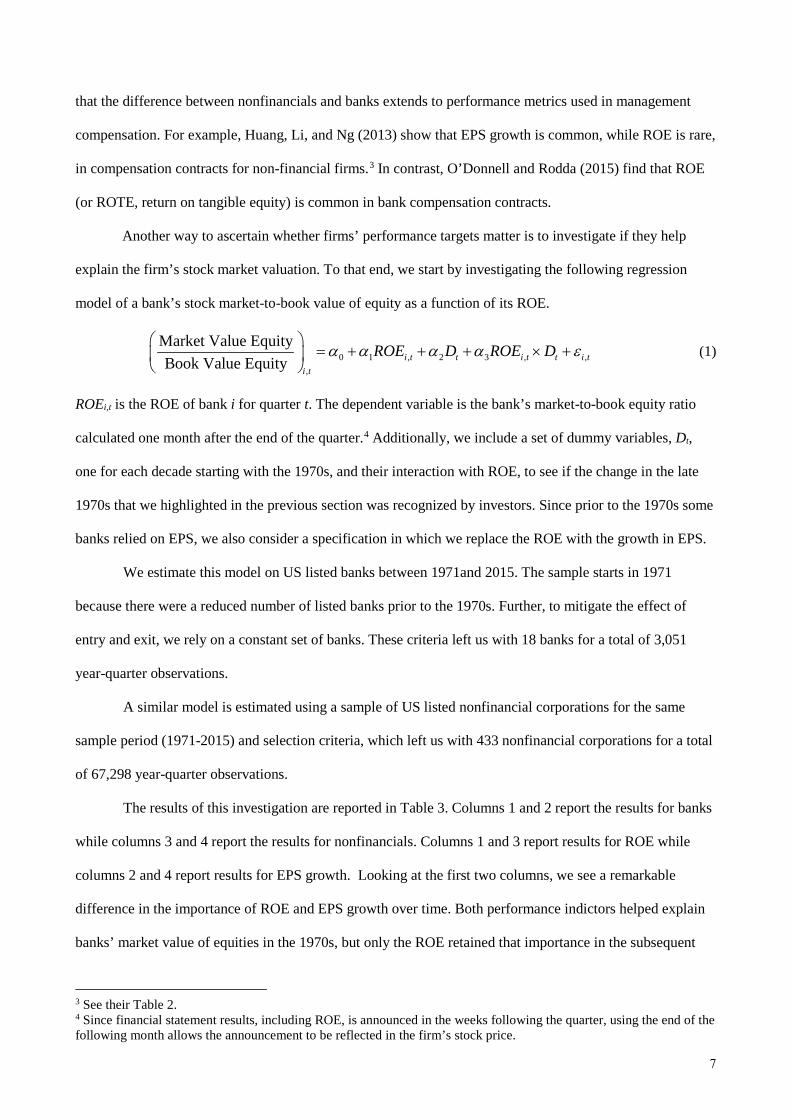
Another way to ascertain whether firms’ performance targets matter is to investigate if they help

explain the firm’s stock market valuation. To that end, we start by investigating the following regression

model of a bank’s stock market-to-book value of equity as a function of its ROE.

0 1 , 2 3 , ,,

Market Value EquityBook Value Equity i t t i t t i t

i t

ROE D ROE Dα α α α ε

= + + + × +

(1)

ROEi,t is the ROE of bank i for quarter t. The dependent variable is the bank’s market-to-book equity ratio

calculated one month after the end of the quarter.4 Additionally, we include a set of dummy variables, Dt,

one for each decade starting with the 1970s, and their interaction with ROE, to see if the change in the late

1970s that we highlighted in the previous section was recognized by investors. Since prior to the 1970s some

banks relied on EPS, we also consider a specification in which we replace the ROE with the growth in EPS.

We estimate this model on US listed banks between 1971and 2015. The sample starts in 1971

because there were a reduced number of listed banks prior to the 1970s. Further, to mitigate the effect of

entry and exit, we rely on a constant set of banks. These criteria left us with 18 banks for a total of 3,051

year-quarter observations.

A similar model is estimated using a sample of US listed nonfinancial corporations for the same

sample period (1971-2015) and selection criteria, which left us with 433 nonfinancial corporations for a total

of 67,298 year-quarter observations.

The results of this investigation are reported in Table 3. Columns 1 and 2 report the results for banks

while columns 3 and 4 report the results for nonfinancials. Columns 1 and 3 report results for ROE while

columns 2 and 4 report results for EPS growth. Looking at the first two columns, we see a remarkable

difference in the importance of ROE and EPS growth over time. Both performance indictors helped explain

banks’ market value of equities in the 1970s, but only the ROE retained that importance in the subsequent

3 See their Table 2. 4 Since financial statement results, including ROE, is announced in the weeks following the quarter, using the end of the following month allows the announcement to be reflected in the firm’s stock price.

8

decades. In contrast, the importance of the EPS declined in all of the subsequent decades. With the exception

of D80 × ROE, which is negative and significant, that interaction is not statistically different from zero for all

of the remaining decades. In contrast, Dt × EPS is negative and statistically different from zero in all decades

after the 1980s. Further, as seen from the p values reported at the bottom of the table we can reject the

hypothesis ROE+ Dt × ROE = 0 for all decades between the 1980s and 2010s. In contrast, we cannot reject

the hypothesis EPS + Dt × EPS = 0 for all those decades.

Turning our attention to columns 3 and 4, we see one important difference. As with banks, ROE and

EPS growth help explain the market value of nonfinancial corporations’ equities in the 1970s. Also, as with

banks, ROE retained its importance in subsequent decades. However, in contrast to banks, we do not see that

EPS growth became less important with the passage of time. Note that Dt × EPS is not statistically

significant for any of the decades after the 1980s.

The difference in the importance of ROE and EPS growth over time among banks appears to be in

line with the anecdotal evidence we presented in the previous section on banks’ use of ROE as their

preferred metric of performance starting in the late 1970s. The difference in the importance of ROE and EPS

growth for banks and nonfinancials also adds to that assertion. However, it is unclear from that table whether

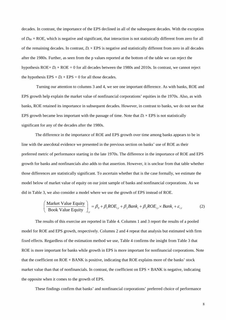
those differences are statistically significant. To ascertain whether that is the case formally, we estimate the

model below of market value of equity on our joint sample of banks and nonfinancial corporations. As we

did in Table 3, we also consider a model where we use the growth of EPS instead of ROE.

0 1 , 2 3 , ,,

Market Value EquityBook Value Equity i t i i t i i t

i t

ROE Bank ROE Bankβ β β β ε

= + + + × +

(2)

The results of this exercise are reported in Table 4. Columns 1 and 3 report the results of a pooled

model for ROE and EPS growth, respectively. Columns 2 and 4 repeat that analysis but estimated with firm

fixed effects. Regardless of the estimation method we use, Table 4 confirms the insight from Table 3 that

ROE is more important for banks while growth in EPS is more important for nonfinancial corporations. Note

that the coefficient on ROE × BANK is positive, indicating that ROE explains more of the banks’ stock

market value than that of nonfinancials. In contrast, the coefficient on EPS × BANK is negative, indicating

the opposite when it comes to the growth of EPS.

These findings confirm that banks’ and nonfinancial corporations’ preferred choice of performance

9

target, ROE and EPS growth, matters at least when it comes to the stock market. In the next section, we

present formal structural models of a bank and a nonfinancial firm that both maximize their shareholders’

value. This analysis allows us to understand how their optimizing behaviors affects their performance based

on ROE and EPS. It provides insights for why banks would have a particular preference for reporting ROE,

rather than EPS, as a performance metric.

4. The Implications of Banks’ and Non-Financial Firms’ Capital Structures for ROE and EPS

This section presents a model of a bank that derives “franchise” value from issuing insured deposits.

The bank pays corporate income taxes and a fixed deposit insurance premium, and it also must meet a

minimum initial regulatory capital requirement. It is assumed that managers choose the bank’s initial equity

capital to maximize the value of its shareholders’ equity in excess of its contributed capital. The main

purpose of this model is to show that a decline in franchise value, which might occur due to increased

competition, leads the bank to reduce its equity capital ratio. When the bank makes this value-maximizing

response, its ROE increases while its EPS growth falls. The implication is that when greater competition

erodes a bank’s charter value, ROE appears to be a better performance metric than EPS growth.

A bank’s behavior is compared to that of a non-financial firm. A non-financial firm maximizes the

value of its excess shareholders’ equity but does not benefit from a government guarantee on its debt: it must

issue debt at a fair promised interest rate. We show that the presence of a government safety net magnifies

the benefit of using ROE as a performance metric. Hence, increasing competition and deposit insurance can

explain why banks have a greater preference for ROE compared to nonfinancial firms.

4.1 Modeling a Bank’s Choice of Capital

Our analysis extends a standard “structural” model of a bank to incorporate franchise value, deposit

insurance, and corporate income taxes. Specifically, we make the following assumptions. At the initial date

0, the bank issues insured deposits of D0 on which it pays the interest rate rd ≤ r, where r is the competitive,

default-free interest rate. As in Merton (1978) and Marcus (1983), a below-competitive deposit interest rate

is a source of “charter” or “franchise” value. Shareholders initially contribute equity capital equal to K0, so

the bank’s date 0 tangible assets equal A0 = D0 + K0. These risky assets have a value that follows the process

10

t

t

dA dt dzA

µ σ= + (3)

where σ > 0 is a constant.

A government regulator sets the bank’s deposit insurance premium at date 0 but is payable by the

bank at the future date T, which also is the time that the regulator audits the bank. Let p be the (continuously-

compounded) annual insurance premium rate per deposit, so that the bank’s total premium to be paid at date

T is DT(epT-1) and the sum of deposits plus premium payable at date T is ( )0

dr p TpTTD e D e += .5 Similar to

Merton (1977), the bank fails and is closed at date T by the regulator if AT < DTepT. The government

regulator/deposit insurer incurs any loss required to pay off the bank’s insured deposits.

Research dating back to Merton (1977) recognizes that fair deposit insurance and capital standards

equate the value of a bank’s insurance premium to the present value of its insurance losses, which equals a

put option written on the bank’s assets with an exercise price equal to its promised payments:

( ) ( )

( ) ( ) ( )

( )2 0 0 1

0 0

Value of Premium Value of Insurance Losses

1 E max ,0

, ,

rT pT rT Q pTT T T

rT pTT

pTT

e D e e D e A

e D e N d K D N d

Put K D D e T

− −

−

− = −

= − − + −

≡ +

(4)

where EQ[·] is the “risk-neutral” expectation,6 ( ) ( )( ) ( )211 0 0 2ln / /rT pT

Td K D e D e T Tσ σ− = + + ,

2 1d d Tσ= − , and Put(A0, X, T) is the value of a Black-Scholes put option written on assets currently worth

A0, having exercise price X, and time until maturity of T. Key to equation (4) is that, given initial capital K0, p

is set fairly when the value of the bank’s insurance premium equals the government’s discounted risk-neutral

expected losses, ( )0 0 , ,pTTPut K D D e T+ .

Let Et denote the value of the bank’s shareholders’ equity at date t. We extend Marcus (1984) to

consider not only charter value that would be lost if the bank fails, but also corporate income taxes, where τ

denotes the bank’s corporate income tax rate. Specifically, we model equity’s date T payoff as

5 This insurance premium is analogous to a credit spread on deposits if deposits were competitively-priced (rd = r) and uninsured. In the absence of deposit insurance and regulation, uninsured depositors would set the credit spread, p, to make the date 0 fair value of their default-risky deposits equal to D0, the amount they contribute initially. 6 The risk-neutral asset return process is / Q

t tdA A rdt dzσ= + .

11

( )0 0

if 0 if

if

pT pTT T T T

T pTT T

pT pTT T T T

A D e C D e AE

A D e

A K D e D e K Aτ

− + ≤=

< − − + + ≤

(5)

where C > 0 denotes the bank’s charter value that is lost if it fails at date T. The first two lines in (5) are

directly from Marcus (1984). The third line equals the bank’s corporate taxes on income after interest and

deposit insurance expense, which equals [AT – (K0+D0×exp((rd+p)T)]τ.7 Therefore earnings after interest and

taxes, when earnings before taxes is positive, equals [AT – (K0+D0×exp((rd+p)T)](1-τ).

A bank’s charter value derives from its market power in being able to issue deposits at below

competitive rates. Note that the initial value from issuing D0 of deposits at below the competitive interest rate

over the period of length T is ( )( )0 1 dr r TD e− −− . Consequently, the value at date T of being able to issue

deposits at all future periods starting at dates T, 2T, 3T, …,∞ is

( )( )( )

( ) ( )0 0 00

11 1 / 11

dd

r r Tr r T rT i cT rT

rTi

eC D e e D D e ee

− −∞− − − × − −

−=

−≡ − = = − −

−∑ (6)

where we define c ≡ r – rd. As detailed in the Appendix, the date 0 value of shareholders’ equity equals

( ) ( ) ( )( ) ( )

( ) ( )0

0 0 0 0 0 2Capital

0 0 1, 0

Value of Mispriced Deposit Insurance Current and Future Charter Value

, , 1 1 dr r TpT rT pT rTT T

rTK T

E K Put K D D e T e D e D e e CN d

K D N d e K D

− −− −

−

− = + − − + − +

− + − +

( ) ( )02,

Value of Corporate Taxes

pTKe N d τ

(7)

where ( ) ( )( )( ) ( )0

211, 0 0 0 2ln / /rT pT

K Td K D e K D e T Tσ σ− = + + + , and

0 02, 1,K Kd d Tσ= − .

Equation (7) shows that the market value of shareholders’ equity equals the sum of initial capital, the value

of a government deposit insurance subsidy, the bank’s current and future charter value, and the value of

corporate taxes.

We illustrate equation (7) by assuming the following parameter values:8

7 We assume deposit insurance premiums are tax-deductible, though they may not be in some countries. 8 Note that the asset volatility of σ = 4% is the average asset volatility estimated by Pennacchi, Vermaelen, and Wolff (2014) for Bank of America, Citigroup, and JPMorgan Chase over the period 2003 to 2012. Using a different method, Berg and Gider (2017) estimate an average asset volatility for a larger group of banks to be 3.5%. The insurance premium of p =10 basis points is comparable to the average rate assessed by the FDIC in recent years. For example for 2017, annual FDIC assessments per year-end domestic deposits was 8.8 basis points.

12

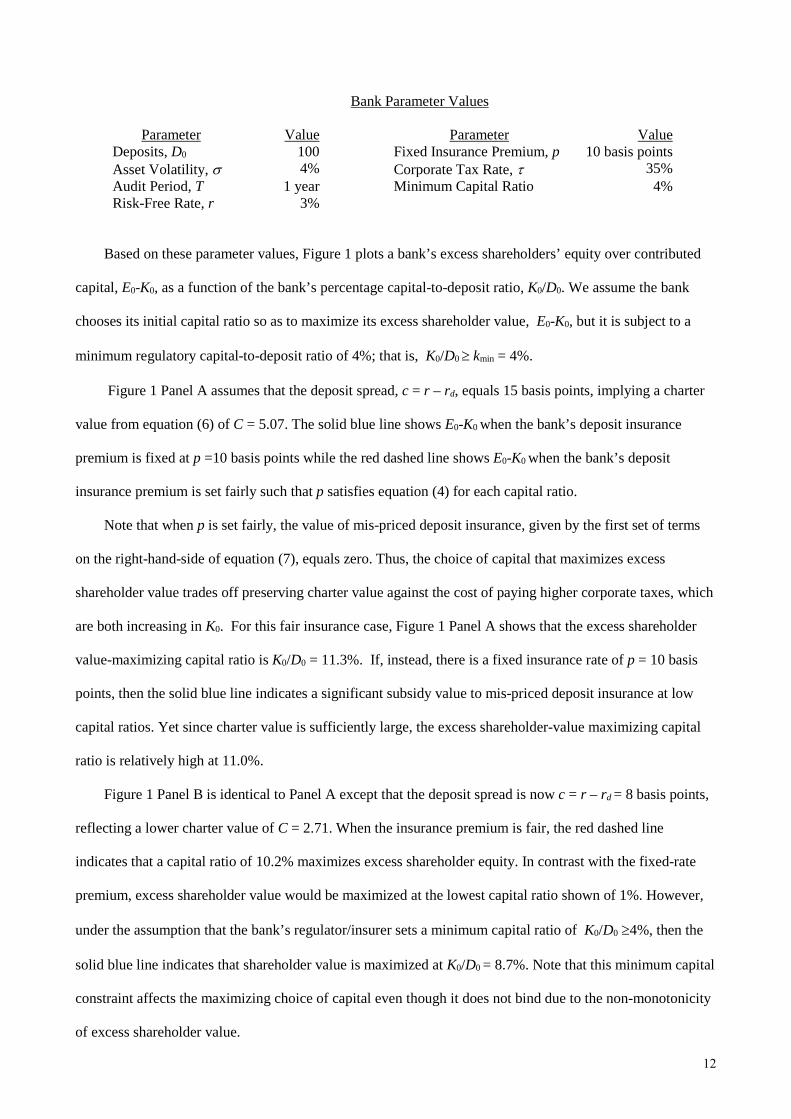
Bank Parameter Values

Parameter Value Parameter Value Deposits, D0 100 Fixed Insurance Premium, p 10 basis points Asset Volatility, σ 4% Corporate Tax Rate, τ 35% Audit Period, T 1 year Minimum Capital Ratio 4% Risk-Free Rate, r 3%

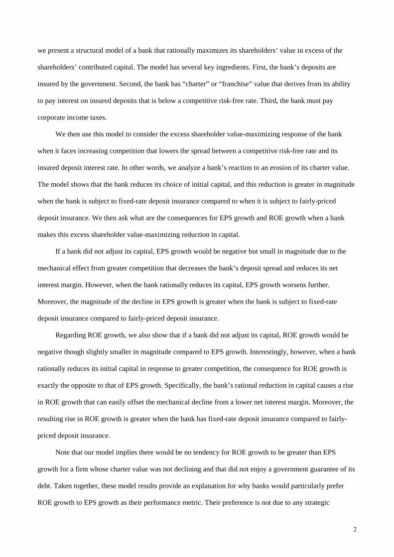
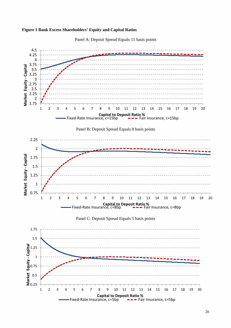
Based on these parameter values, Figure 1 plots a bank’s excess shareholders’ equity over contributed

capital, E0-K0, as a function of the bank’s percentage capital-to-deposit ratio, K0/D0. We assume the bank

chooses its initial capital ratio so as to maximize its excess shareholder value, E0-K0, but it is subject to a

minimum regulatory capital-to-deposit ratio of 4%; that is, K0/D0 ≥ kmin = 4%.

Figure 1 Panel A assumes that the deposit spread, c = r – rd, equals 15 basis points, implying a charter

value from equation (6) of C = 5.07. The solid blue line shows E0-K0 when the bank’s deposit insurance

premium is fixed at p =10 basis points while the red dashed line shows E0-K0 when the bank’s deposit

insurance premium is set fairly such that p satisfies equation (4) for each capital ratio.

Note that when p is set fairly, the value of mis-priced deposit insurance, given by the first set of terms

on the right-hand-side of equation (7), equals zero. Thus, the choice of capital that maximizes excess

shareholder value trades off preserving charter value against the cost of paying higher corporate taxes, which

are both increasing in K0. For this fair insurance case, Figure 1 Panel A shows that the excess shareholder

value-maximizing capital ratio is K0/D0 = 11.3%. If, instead, there is a fixed insurance rate of p = 10 basis

points, then the solid blue line indicates a significant subsidy value to mis-priced deposit insurance at low

capital ratios. Yet since charter value is sufficiently large, the excess shareholder-value maximizing capital

ratio is relatively high at 11.0%.

Figure 1 Panel B is identical to Panel A except that the deposit spread is now c = r – rd = 8 basis points,

reflecting a lower charter value of C = 2.71. When the insurance premium is fair, the red dashed line

indicates that a capital ratio of 10.2% maximizes excess shareholder equity. In contrast with the fixed-rate

premium, excess shareholder value would be maximized at the lowest capital ratio shown of 1%. However,

under the assumption that the bank’s regulator/insurer sets a minimum capital ratio of K0/D0 ≥4%, then the

solid blue line indicates that shareholder value is maximized at K0/D0 = 8.7%. Note that this minimum capital

constraint affects the maximizing choice of capital even though it does not bind due to the non-monotonicity

of excess shareholder value.

13

Finally, Panel C of Figure 1 replicates the analysis of the earlier two panels but with a deposit spread of

c = r – rd = 5 basis points so that charter value is the low level of C = 1.69. Here, under a fair insurance

premium, the red dashed line shows that the capital ratio of 9.3% maximizes excess shareholder value.

However, for the fixed-rate insurance premium, the solid blue line shows that the binding capital ratio of

4.0% maximizes excess shareholder value.

The main result from the three panels in Figure 1 is that lower charter value causes banks to reduce their

excess shareholder value-maximizing capital ratio, and the magnitude of this capital reduction is greater

when banks have fixed-rate deposit insurance rather than fairly-priced deposit insurance. Unlike fairly-

priced deposit insurance, fixed rate insurance does not penalize banks for reducing capital, so that the bank

captures a greater government safety-net subsidy when reducing capital.

4.2 Modeling a Non-financial Firm’s Choice of Equity

Our modeling of a non-financial corporation is similar to that of banks but with three important

differences. First, the firm does not benefit from being able to issue debt at a below competitive rate as a

bank does with its retail deposits. Therefore, we assume that the certainty-equivalent interest rate that a non-

financial firm pays on its debt is rd = r. It is assumed that the non-financial firm has future charter value, C,

but this charter value derives from other sources such as proprietary technology, patents, or brand identity

and is independent of the interest rate on its debt. Second, the government does not guarantee the debt of a

nonfinancial firm. Rather than paying a deposit insurance premium, the parameter p is now interpreted as the

fair credit spread that investors require on the non-financial firm’s default-risky debt so that its initial value

equals D0. Third, the non-financial firm is not subject to a minimum regulatory capital constraint.

With these changes, our model of a non-financial firm is similar to Merton (1974) but with the addition

of charter value and corporate income taxes. The firm’s value of shareholder’s equity in excess of

contributed capital satisfies

( ) ( ) ( ) ( )( ) ( )0 00 0 2 0 0 1, 0 0 2,Capital Future Charter Value Value of Corporate Taxes

r p TrT rTK KE K e CN d K D N d e K D e N d τ+− − − = − + − +

(8)

where ( ) ( )( ) ( )211 0 0 0 2ln / /pTd K D D e T Tσ σ = + + , 2 1d d Tσ= − ,

( ) ( )( )( )( ) ( )0

211, 0 0 0 0 2ln / /r p TrT

Kd K D e K D e T Tσ σ+− = + + + ,

0 02, 1,K Kd d Tσ= − ,

14

and the firm’s fair credit spread on its debt is the value of p that satisfies the condition

( ) ( ) ( ) ( )( )( )

0 0 2 0 0 1

0 0 0

1

, ,

pT pT

r p T

D e D e N d K D N d

Put K D D e T+

− = − − + −

≡ + (9)

For the case of non-financial firms, the shareholder value-maximizing choice of contributed capital, K0,

is an interior value that trades off better protection of charter value for higher corporate taxes. Consequently,

non-financial firms with a higher exogenous charter value will tend to choose a higher equity to debt ratio.

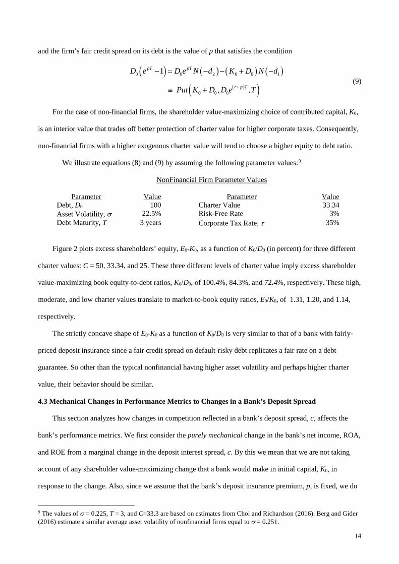
We illustrate equations (8) and (9) by assuming the following parameter values:9

NonFinancial Firm Parameter Values

Parameter Value Parameter Value Debt, D0 100 Charter Value 33.34 Asset Volatility, σ 22.5% Risk-Free Rate 3% Debt Maturity, T 3 years Corporate Tax Rate, τ 35%

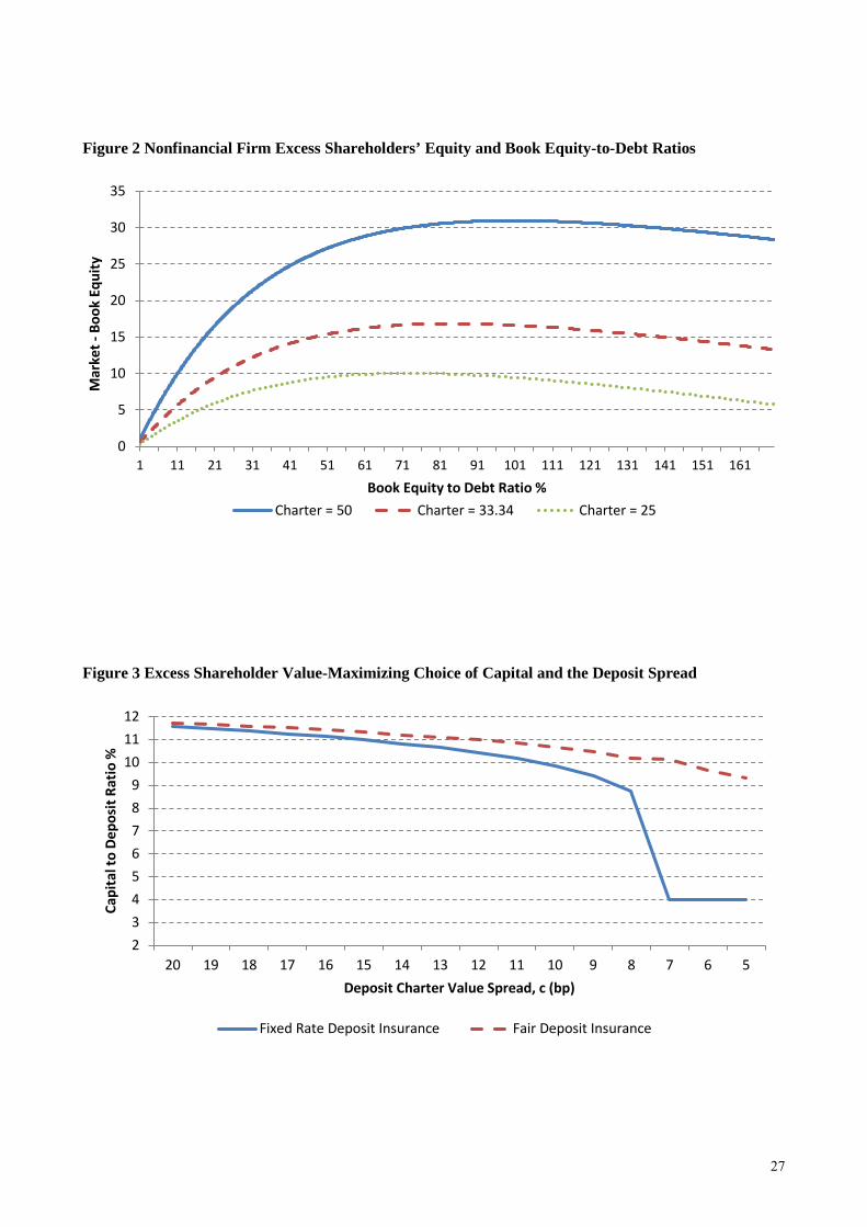
Figure 2 plots excess shareholders’ equity, E0-K0, as a function of K0/D0 (in percent) for three different

charter values: C = 50, 33.34, and 25. These three different levels of charter value imply excess shareholder

value-maximizing book equity-to-debt ratios, K0/D0, of 100.4%, 84.3%, and 72.4%, respectively. These high,

moderate, and low charter values translate to market-to-book equity ratios, E0/K0, of 1.31, 1.20, and 1.14,

respectively.

The strictly concave shape of E0-K0 as a function of K0/D0 is very similar to that of a bank with fairly-

priced deposit insurance since a fair credit spread on default-risky debt replicates a fair rate on a debt

guarantee. So other than the typical nonfinancial having higher asset volatility and perhaps higher charter

value, their behavior should be similar.

4.3 Mechanical Changes in Performance Metrics to Changes in a Bank’s Deposit Spread

This section analyzes how changes in competition reflected in a bank’s deposit spread, c, affects the

bank’s performance metrics. We first consider the purely mechanical change in the bank’s net income, ROA,

and ROE from a marginal change in the deposit interest spread, c. By this we mean that we are not taking

account of any shareholder value-maximizing change that a bank would make in initial capital, K0, in

response to the change. Also, since we assume that the bank’s deposit insurance premium, p, is fixed, we do

9 The values of σ = 0.225, T = 3, and C=33.3 are based on estimates from Choi and Richardson (2016). Berg and Gider (2016) estimate a similar average asset volatility of nonfinancial firms equal to σ = 0.251.

15

not consider any change in the bank’s cost of funds beyond that given by the change in the deposit rate that is

a result of the change in spread. In other words, we only consider ∂c = - ∂rd which increases net income by

increasing the net interest margin, (r – rd).

Define the bank’s net income after interest expense and taxes as NI ≡ [AT – (K0+D0×exp((rd+p)T)](1-τ).

Obviously, net income is positively related to the deposit insurance spread:

( ) ( )0 1 0r p c TNI TD ec

τ+ −∂= − >

∂(10)

Assuming there are no distributions of dividends from net income, the change in NI produces a one-for-one

change in capital, K, and assets, A. That is, ∂K/∂c = ∂A/∂c = ∂NI/∂c. Note that the return on equity (ROE) and

the return on assets (ROA) equal NI/K and NI/A, respectively. First consider how a change in c affects ROE:

2 2 2

ROE /NI K NI NIK NI K NINI K K NI NIc c c c

c c K K K c

∂ ∂ ∂ ∂− −∂ ∂ − ∂ ∂ ∂ ∂ ∂= = = = ∂ ∂ ∂

(11)

Similarly,

2

ROA /NI A A NI NIc c A c

∂ ∂ − ∂ = = ∂ ∂ ∂ (12)

Now since ( ) ( )2 3/ / 2 /x NI x x x NI x ∂ − ∂ = − − < 0 when x > NI, we see that as long as capital and

assets are greater than net income and K < A, then the absolute change in ROE to a change in c is larger than

the absolute change in ROA to a change in c.

Next, consider how a change in c affects the proportional change in ROE.

2

lnln ROE / 1 ln

NIK NI K K K NI NI K NI NI K NI NIK

c c NI c NI K c K NI c K c

∂ ∂ ∂ − ∂ − ∂ − ∂ = = = = = ∂ ∂ ∂ ∂ ∂ ∂ (13)

Similarly

lnln ROA ln

NIA NI NIA

c c A c

∂ ∂ − ∂ = = ∂ ∂ ∂ (14)

16

Now since ( ) 2/ / / 0x NI x x NI x∂ − ∂ = > when NI > 0, we see that as long as capital and assets are

greater than net income and K < A, then the proportional change in ROE to a change in c is smaller than the

proportional change in ROA to a change in c.

It is interesting that ∂lnNI/∂c is earnings growth or “growth in earnings per share (EPS)” which is the

most common performance benchmark for non-financial firms. Thus, if a bank uses growth in ROE,

∂lnROE/∂c =[(K – NI)/K]∂lnNI/∂c, it is less sensitive to performance than growth in EPS. Moreover, by

reducing K for a given amount of earnings, the bank can further reduce the sensitivity of ROE growth to

performance. From a purely marketing point of view, a bank might want to decrease its preferred

benchmark’s sensitivity to performance when its performance is declining.

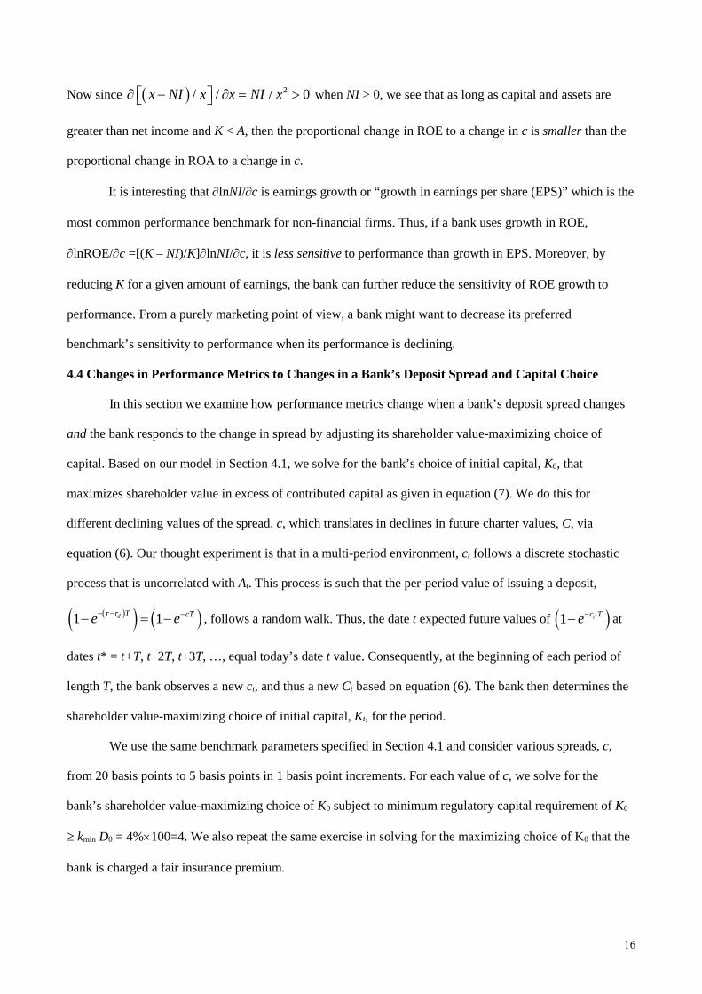
4.4 Changes in Performance Metrics to Changes in a Bank’s Deposit Spread and Capital Choice

In this section we examine how performance metrics change when a bank’s deposit spread changes

and the bank responds to the change in spread by adjusting its shareholder value-maximizing choice of

capital. Based on our model in Section 4.1, we solve for the bank’s choice of initial capital, K0, that

maximizes shareholder value in excess of contributed capital as given in equation (7). We do this for

different declining values of the spread, c, which translates in declines in future charter values, C, via

equation (6). Our thought experiment is that in a multi-period environment, ct follows a discrete stochastic

process that is uncorrelated with At. This process is such that the per-period value of issuing a deposit,

( )( ) ( )1 1dr r T cTe e− − −− = − , follows a random walk. Thus, the date t expected future values of ( )*1 tc Te−− at

dates t* = t+T, t+2T, t+3T, …, equal today’s date t value. Consequently, at the beginning of each period of

length T, the bank observes a new ct, and thus a new Ct based on equation (6). The bank then determines the

shareholder value-maximizing choice of initial capital, Kt, for the period.

We use the same benchmark parameters specified in Section 4.1 and consider various spreads, c,

from 20 basis points to 5 basis points in 1 basis point increments. For each value of c, we solve for the

bank’s shareholder value-maximizing choice of K0 subject to minimum regulatory capital requirement of K0

≥ kmin D0 = 4%×100=4. We also repeat the same exercise in solving for the maximizing choice of K0 that the

bank is charged a fair insurance premium.

17

The result of this exercise is given in Figure 3. Similar to what was illustrated in Figure 1, we see

that a lower deposit spread, reflecting a lower charter value, reduces a bank’s choice of capital whether or

not the bank has fairly-priced deposit insurance (dashed red line) or fixed-rate deposit insurance (solid blue

line). Though the fixed-rate insurance bank always chooses lower capital than that of the fair insurance bank,

there is not much difference when spreads are high. However, the difference becomes increasingly larger

until the fixed-rate insurance bank chooses the minimum capital level, kmin = 4%, which occurs when the

deposit spread, c, equals 7 basis points (a value of C = 2.37).

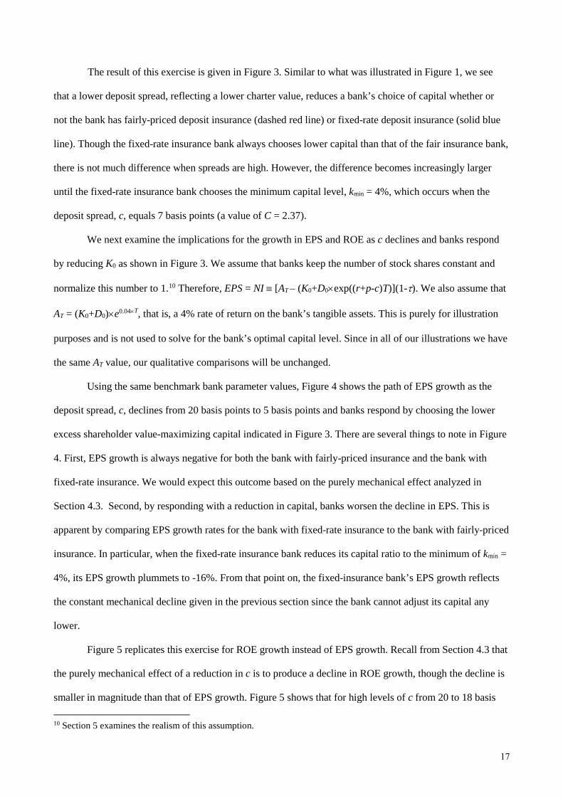
We next examine the implications for the growth in EPS and ROE as c declines and banks respond

by reducing K0 as shown in Figure 3. We assume that banks keep the number of stock shares constant and

normalize this number to 1.10 Therefore, EPS = NI ≡ [AT – (K0+D0×exp((r+p-c)T)](1-τ). We also assume that

AT = (K0+D0)×e0.04×T, that is, a 4% rate of return on the bank’s tangible assets. This is purely for illustration

purposes and is not used to solve for the bank’s optimal capital level. Since in all of our illustrations we have

the same AT value, our qualitative comparisons will be unchanged.

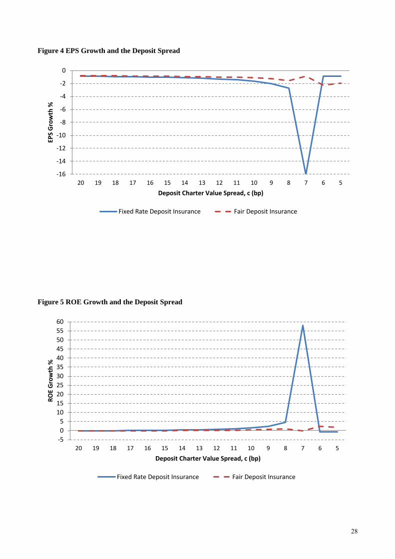
Using the same benchmark bank parameter values, Figure 4 shows the path of EPS growth as the

deposit spread, c, declines from 20 basis points to 5 basis points and banks respond by choosing the lower

excess shareholder value-maximizing capital indicated in Figure 3. There are several things to note in Figure

4. First, EPS growth is always negative for both the bank with fairly-priced insurance and the bank with

fixed-rate insurance. We would expect this outcome based on the purely mechanical effect analyzed in

Section 4.3. Second, by responding with a reduction in capital, banks worsen the decline in EPS. This is

apparent by comparing EPS growth rates for the bank with fixed-rate insurance to the bank with fairly-priced

insurance. In particular, when the fixed-rate insurance bank reduces its capital ratio to the minimum of kmin =

4%, its EPS growth plummets to -16%. From that point on, the fixed-insurance bank’s EPS growth reflects

the constant mechanical decline given in the previous section since the bank cannot adjust its capital any

lower.

Figure 5 replicates this exercise for ROE growth instead of EPS growth. Recall from Section 4.3 that

the purely mechanical effect of a reduction in c is to produce a decline in ROE growth, though the decline is

smaller in magnitude than that of EPS growth. Figure 5 shows that for high levels of c from 20 to 18 basis

10 Section 5 examines the realism of this assumption.

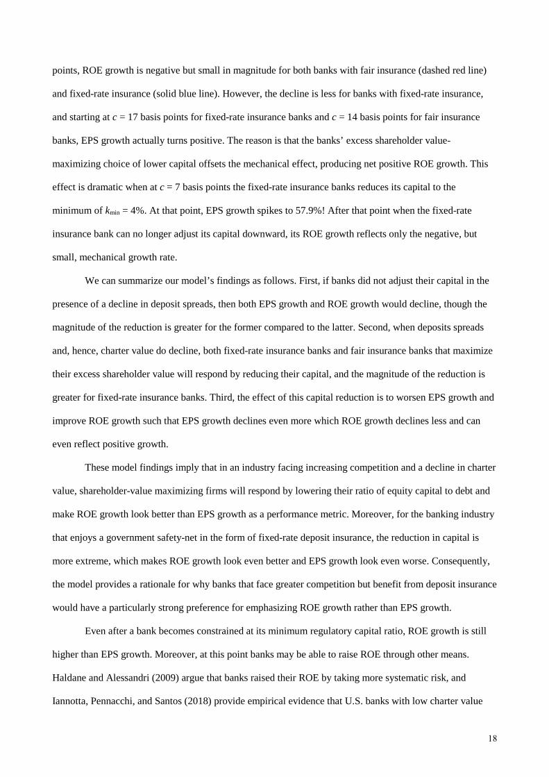
18

points, ROE growth is negative but small in magnitude for both banks with fair insurance (dashed red line)

and fixed-rate insurance (solid blue line). However, the decline is less for banks with fixed-rate insurance,

and starting at c = 17 basis points for fixed-rate insurance banks and c = 14 basis points for fair insurance

banks, EPS growth actually turns positive. The reason is that the banks’ excess shareholder value-

maximizing choice of lower capital offsets the mechanical effect, producing net positive ROE growth. This

effect is dramatic when at c = 7 basis points the fixed-rate insurance banks reduces its capital to the

minimum of kmin = 4%. At that point, EPS growth spikes to 57.9%! After that point when the fixed-rate

insurance bank can no longer adjust its capital downward, its ROE growth reflects only the negative, but

small, mechanical growth rate.

We can summarize our model’s findings as follows. First, if banks did not adjust their capital in the

presence of a decline in deposit spreads, then both EPS growth and ROE growth would decline, though the

magnitude of the reduction is greater for the former compared to the latter. Second, when deposits spreads

and, hence, charter value do decline, both fixed-rate insurance banks and fair insurance banks that maximize

their excess shareholder value will respond by reducing their capital, and the magnitude of the reduction is

greater for fixed-rate insurance banks. Third, the effect of this capital reduction is to worsen EPS growth and

improve ROE growth such that EPS growth declines even more which ROE growth declines less and can

even reflect positive growth.

These model findings imply that in an industry facing increasing competition and a decline in charter

value, shareholder-value maximizing firms will respond by lowering their ratio of equity capital to debt and

make ROE growth look better than EPS growth as a performance metric. Moreover, for the banking industry

that enjoys a government safety-net in the form of fixed-rate deposit insurance, the reduction in capital is

more extreme, which makes ROE growth look even better and EPS growth look even worse. Consequently,

the model provides a rationale for why banks that face greater competition but benefit from deposit insurance

would have a particularly strong preference for emphasizing ROE growth rather than EPS growth.

Even after a bank becomes constrained at its minimum regulatory capital ratio, ROE growth is still

higher than EPS growth. Moreover, at this point banks may be able to raise ROE through other means.

Haldane and Alessandri (2009) argue that banks raised their ROE by taking more systematic risk, and

Iannotta, Pennacchi, and Santos (2018) provide empirical evidence that U.S. banks with low charter value

19

and low capital took systematic risk that was relatively high compared to banks with high charter value and

high capital.

5. Evidence in Support of the Model’s Assumptions

In this section, we present supporting evidence for four important assumptions we made in our

model, namely (i) that the insurance premiums charged to banks are not risk based, (ii) that firms do not

actively manage the number of their shares in order to improve their EPS-based performance metrics, (iii)

that banks’ charter value declined over time, and finally (iv) that banks’ capital-to-assets ratio declined over

time.

5.1 Deposit Insurance Premiums and Bank Risk

A key assumption of our model is that banks pay an insurance premium that is either fixed or does not fully

reflect their risk of failure. Indeed, up until 1993, the nominal (and effective) rate banks paid the FDIC was

completely unrelated to their risk, notwithstanding the fact that the insurance coverage increased by a

multiple of 20 (from $5,000 to $100,000).11

From 1935 until 1950, the FDIC by law charged a flat assessment rate of 8.33 basis points against an

assessment base of domestic deposits, the equivalent of 8.33 cents for every $100 of deposits. As the

insurance fund kept growing, and following calls from the industry for insurance payments’ relief, Congress

passed the Federal Deposit Insurance Act of 1950 which gave a credit to banks of about 60 percent. As a

result, the effective assessment rate was approximately halved. However, as losses from failures mounted

during the early 1980s, credits to banks declined until they ceased altogether in 1985, at which time the

effective assessment rate returned to 8.33 basis points. Further, as banking crisis deepened in the late 1980s,

assessment rates rose considerably, reaching 23 bps by July 1991.12

It was only in 1991 that the FDIC changed the flat-rate assessment system to one based on the bank’s

risk to the deposit insurance fund, taking into account a variety of risk measurements, the likelihood of loss

to the fund, and the fund’s revenue needs. While conceptually this was a significant departure from the

historic flat-rate practice, effective insurance premiums remained only mildly linked to bank risk. The new

11 Congress increased the deposit insurance coverage level five times from 1950 to 1980: from $5,000 to $10,000 in 1950, to $15,000 in 1966, to $20,000 in 1969, to $40,000 in 1974, and to $100,000 in 1980. In 2008, that limit was further increased to $250,000. 12 Following the large number of bank failures in the 1980s and the depletion of FDIC insurance fund, the 1989 Financial Institutions Reform, Recovery and Enforcement Act mandated that premiums be set to achieve a ratio of 1.25 percent of reserves to total insured deposits.

20

system, which was introduced by Federal Deposit Insurance Corporation Improvement Act of 1991, began to

be implemented in January of 1993. Banks were assigned to a nine-cell matrix depending on their

capitalization (well capitalized, adequately capitalized, or undercapitalized) and on their primary federal

regulator's composite rating (rating 1 or 2, rating 3, or rating 4 or 5) and depending on their cell charged one

out of five possible risk premiums which ranged from 23 to 31 bps.

This architecture remained in place with only minor changes in the level of the premiums up until

2007. 13 In principle, it gave the FDIC the opportunity to charge banks a limited number of possible

premiums based on risk. However, in practice it did not provide much differentiation across banks. From

1996 to 2006, well over 90 percent of banks were categorized in the lowest-risk category (well capitalized

with a rating of 1 or 2), implying that they paid no insurance premium on their deposits (Pennacchi 2010).

The Federal Deposit Insurance Reform Act of 2005 instituted an important change with regards to

the setting of insurance premiums – it gave the FDIC the possibility of charging an insurance premium to

banks classified as the least risky even when the deposit insurance fund was above its target.14 Soon after,

on January 1, 2007, the FDIC replaced the nine-cell matrix with a system of 4 risk categories. Additionally,

the FDIC set a range for the premiums applicable to the safest institutions, which varied between 5 and 7

bps. Institutions classified in the remaining risk categories were assessed a premium of 10, 28 and 43 bps,

respectively.

Starting in April of 2009, the FDIC began to factor in other liability variables, including unsecured

debt and brokered deposits, when setting insurance premiums. Further, starting in April of 2011, the FDIC

added to the four-risk categories a new category for the large and highly complex institutions.

In sum, up until 1993 US banks were indeed charged a flat premium. Since then, there have been

several changes aimed at making the premiums risk based. However, as we documented above the effective

risk premiums banks pay continues to be only insipidly linked to their risk

5.2 Number of Shares and Firms’ Performance

A second important assumption of our model is that the number of shares is either constant or that firms do

not actively manage the number of their shares to “improve” their performance as captured in their EPS. To

13 A revision in July of 1995 gave the FDIC the possibility of charging six different premiums to banks, ranging from 4 to 31 bps, and another one in January of 1996 lowered all of the premiums by 4 bps. 14 That Act made a second important change – it allowed the target ratio of reserves to total insurance deposits to vary between 1.15 percent and 1.50 percent as opposed to the 1.25 percent hard ratio set in 1989.

21

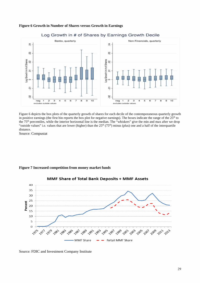
examine the realism of this assumption, we started by computing box plots for the growth in the number of

shares over the quarter for each decile of the distribution of the contemporaneous (positive) earnings growth.

We also create a separate bin category for when earnings are negative. We rely on the same set of banks and

nonfinancial corporations we used in Section 3. The results of this exercise are reported in Figure 6. The

boxes indicate the range of the 25th to the 75th percentiles of share growth obervations, while the interior horizontal line

is the median. The “whiskers” give the min and max after we drop “outside values” i.e. values that are lower (higher)

than the 25th (75th) minus (plus) one and a half of the interquartile distance.

As we can see from the figure, there is no clear monotonic relationship consistent with an active

management of the number of shares to improve the growth in EPS. Instead, there appears to exist a convex

relationship between the growth in the number of shares and the growth in earnings for both banks and

nonfinancials. The median growth in the number of shares for each bin is either zero or positive.15

To investigate the relationship between earnings growth and share growth more formally, we

estimate a regression model where the dependent variable is the quarterly share growth rate. The explanatory

variables are five indicators that capture the contemporaneous change in quarterly earnings: one to account

for negative earnings (NEARN) and the remaining four to account for each quartile of the distribution of

positive changes (PEARNj, with j=1…4). The omitted group is the quartile with the highest growth in

earnings.16

,0 1 ; , 1 ; , 1 ,

, 1

Sharesln

Sharesi t

i t t j i t t i ti t

NEARN PEARNjβ β β ε− −−

= + + +

(15)

The results of this exercise are reported in Table 5. Models 1 and 2 report are a pooled regression

while models 3 and 4 report a regression with firm fixed effects. A quick inspection of all models confirms

our previous insight that firm managers do not appear to actively manage the number of shares in order to

improve performance as captured by their EPS growth. While the coefficients on the lower quartiles of the

earnings growth are negative and statistically significant, they are all smaller than the constant term. In other

words, even when firms experience low earnings growth they do not reduce the number of shares in order to

generate higher EPS growth rates.

15 The mean of share growth is also positive for each decile, except for the first decile (1) for banks which is -0.0006. 16 Using deciles as opposed to quartiles yields similar results.

22

In sum, as in the case of our assumption on flat insurance premiums, the evidence on the number of

shares supports of assumption that neither banks nor financial corporations manage their shares in order to

improve the growth in the EPS in periods they experience low earning growth.

5.3 Banks’ Charter Value over Time

Another assumption we need to justify for our model to truly explain banks’ decision to switch to a ROE-

based target is a decline in their charter value over time. A potential source of erosion in banks’ charter value

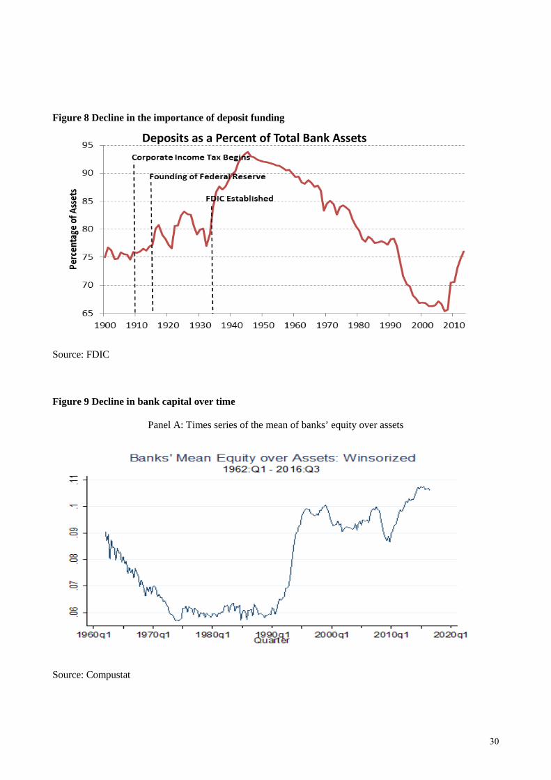
is an increase in competition from non-bank financial intermediaries. As we can see from Figure 7, starting

in the 1970’s, higher inflation and Regulation Q limits on deposit interest rates allowed money market funds

to begin gaining market share. The growth of this industry was important because it competed directly for

one of the banks’ most important sources of charter value: deposit funding. Indeed, as we can see from

Figure 8, which reports the share of deposit funding banks used over time, there was a decline in the relative

importance of deposit funding going back to the mid-1940s. However, that trend appears to have accelerated

in the mid-1970s, coinciding with the growth of the money markets and with the beginning of banks’

adoption of an ROE target.

Another potential source of erosion in banks’ charter value is an increase in competition from within

the banking industry. For decades, state laws on branching and out-of-state entry severely limited

competition in the US banking industry. However, starting in the 1980s many states lifted restrictions on

branching within their borders and began to permit out-of-state institutions to acquire their banks. This

process of deregulation culminated with the Riegle-Neal Interstate Banking and Branching Efficiency Act of

1994 which eliminated most restrictions on interstate bank acquisitions and made interstate branching

possible for the first time in seventy years. Several studies, including Kroszner and Strahan (1999), Jayaratne

and Strahan (1996), and Stiroh and Strahan (2003), have documented an increase in bank competition

following the liberalization of state branching and interstate banking laws.

5.4 Banks’ Capital-to-Asset Ratios over Time

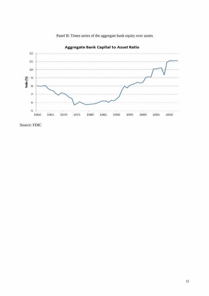
A final implication of our model which is consistent with banks’ adoption of an ROE target is a decline in

bank capital. As we can see from Figure 9 which plots the equity capital-to-assets ratio for the US banking

industry, there was a downward trend in capital at least since the early 1960s, which stopped by the mid-

23

1970s. After that, the capital-to-assets ratio remained somewhat constant up until the implementation of

Basel I in the early 1990s when it began an upward trend.

6. Conclusions

This paper addresses the puzzling question of why banks target ROE while nonfinancial firms target

EPS, and why this difference started in the late 1970s. Its explanation is based on two specific features of

the banking industry. First, banks began to face high levels of competition, particularly for their retail

deposits, during the 1970s. This more aggressive competition eroded banks’ charter values. Second, different

from other firms, banks benefit from a safety net in the form of government deposit insurance that is largely

insensitive to a bank’s risk of failure.

Our model shows that a loss of charter value along with fixed-rate deposit insurance would lead a

bank to reduce its capital ratio when it maximize its shareholders’ equity value in excess of its shareholders’

contributed capital. A by-product of this rational reaction to greater competition is that the bank’s EPS

growth shows a substantial decline while its ROE growth displays a significant rise. Consequently, if the

bank wanted to paint a rosy picture of its performance, it would undoubtedly choose ROE as its target rather

than EPS. The popularity of ROE in bank compensation contracts and in communications with investors is

consistent with this choice.

Note that our model predicts that banks would be especially resistant to post-financial crisis

regulation, such as Basel III, that is gradually forcing them to increase their capital. The model shows that

higher required capital reduces the value of a bank’s shareholders’ equity when the bank has low charter

value and, therefore, finds the minimum capital to be its best choice. A by-product of higher capital is

downward pressure on the bank’s ROE. An implication of our analysis is that the typical bank’s performance

based on ROE is now worse than if it were based on EPS. If minimum capital standards continue to rise, we

might expect that banks will de-emphasize ROE in favor of EPS.

Finally, our paper provides a “positive” theory for banks focus on ROE. Whether there is a

“normative” rationale for regulation to impose a different performance metric is left for future research.

24

Appendix: Derivation of the Model

This appendix derives equation (7) of the text. Note from the payoff of equity in equation (5) that it

de-composed into three components: 1) a call option written on the bank’s assets with an exercise price of

pTTD e ; 2) a digital option that pays C when the call option in 1) is in the money; and 3) -τ times the value of

a call option written on the bank’s assets with an exercise price of 0pT

TD e K+ .

Valuing the above three components using standard Black-Scholes option valuation and noting that

the date 0 value of tangible assets is A0 = K0 + D0, the date 0 value of shareholders’ equity is

( ) ( ) ( ) ( )( ) ( ) ( ) ( )

( ) ( ) ( ) ( )( ) ( ) ( ) ( )

0 0

0 0

0 0 0 1 2 2

0 0 1, 0 2,

0 0 0 0 1 2 2

0 0 1, 0 2,

rT pT rTT

rT pTK T K

rT pT rTT

rT pTK T K

E K D N d e D e N d e CN d

K D N d e K D e N d

K D K D N d e D e N d e CN d

K D N d e K D e N d

τ

τ

− −

−

− −

−

= + − +

− + − + = + − + − − +

− + − +

(A.1)

Adding and subtracting the value of premiums, ( ) ( ) ( )01 1dr r TrT pT pTTe D e D e e− −− − = − , from the right-hand-

side of (A.1) and re-arranging terms we obtain:

( ) ( ) ( ) ( )( )( ) ( )

( ) ( ) ( ) ( )0 0

0 0 2 0 0 1

0 2

0 0 1, 0 2,

1

1 d

rT pT rT pTT T

r r T rT

rT pTK T K

E K e D e N d K D N d e D e

D e e CN d

K D N d e K D e N d τ

− −

− − −

−

= + − − + − − −

+ − +

− + − +

(A.2)

By noting that the second and third terms on the right-hand-side of (A.2) equal the value of a put

option written on bank assets with an exercise price of DTepT, we obtain equation (7) in the text.

25

References

Admati, A., P. DeMarzo, M. Hellwig, and P. Pfleiderer, 2013. “Fallacies, Irrelevant Facts, and Myths in the

Discussion of Capital Regulation: Why Bank Equity is Not Socially Expensive,” working paper.

Begenau, J. and E. Stafford. 2016. “Inefficient Banking,” Harvard University working paper.

Berg, T. and J. Gider. 2017. “What Explains the Difference in Leverage Between Banks and Nonbanks?,”

Journal of Financial and Quantitative Analysis 52, 2677-2702.

Choi, J. and M. Richardson, 2016. “The Volatility of a Firm’s Assets and the Leverage Effect,” Journal of

Financial Economics 121, 254-277.

Floyd, E., N. Li, and D. Skinner, 2015. “Payout Policy Through the Financial Crisis: The Growth of

Repurchases and the Resilience of Dividends,” Journal of Financial Economics 118, 299-316.

Haldane, A. and P. Alessandri, 2009. “Banking on the State,” Bank of England working paper.

Huang, Y., N. Li, and J. Ng, 2013. “Performance Measures in CEO Annual Bonus Contracts,” working

paper, University of Texas at Austin.

Iannota, G., G. Pennacchi, and J. Santos, 2018. “Risk-Based Regulation and Systematic Risk Incentives,”

working paper.

Jayaratne, J. and P.E. Strahan (1996). “The Finance-Growth Nexus: Evidence from Bank Branch

Deregulation.” Quarterly Journal of Economics 111, 639-670.

Kroszner, R.S. and P.E. Strahan (1999). “What Drives Deregulation? Economics and Politics of the

Relaxation of Bank Branching Restrictions.” Quarterly Journal of Economics 114, 1437-1467.

Marcus, A., 1984. “Deregulation and Bank Financial Policy,” Journal of Banking and Finance 8, 557-565.

Merton, R., 1974. “On the Pricing of Corporate Debt: The Risk Structure of Interest Rates,” Journal of

Finance 29, 449-470.

Merton, R., 1978. “On the Cost of Deposit Insurance When There Are Surveillance Costs,” Journal of

Business 51, 439-452.

O’Donnell, S. and D. Rodda, 2015. “New Realities of Executive Compensation in the Banking Industry: The

Importance of Balancing Differing Perspectives,” White Paper MER-006, Meridian Compensation

Partners.

Pennacchi, G., 2010. “Deposit Insurance Reform,” Chapter 1 in Public Insurance and Private Markets,

Jeffrey R. Brown, editor, AEI Press, Washington, D.C.

Pennacchi, G., T. Vermaelen, and C. Wolff, 2014. “Contingent Capital: The Case of COERCs,” Journal of

Financial and Quantitative Analysis 49, 541-574.

Stiroh, K.J. and P.E. Strahan (2003). “Competitive Dynamics of Deregulation: Evidence from U.S.

Banking,” Journal of Money, Credit and Banking 35(5), 801-828.

26

Figure 1 Bank Excess Shareholders’ Equity and Capital Ratios

Panel A: Deposit Spread Equals 15 basis points

Panel B: Deposit Spread Equals 8 basis points

Panel C: Deposit Spread Equals 5 basis points

1.752

2.252.5

2.753

3.253.5

3.754

4.254.5

1 2 3 4 5 6 7 8 9 10 11 12 13 14 15 16 17 18 19 20

Mar

ket

Equi

ty -

Capi

tal

Capital to Deposit Ratio %Fixed-Rate Insurance, c=15bp Fair Insurance, c=15bp

0.75

1

1.25

1.5

1.75

2

2.25

1 2 3 4 5 6 7 8 9 10 11 12 13 14 15 16 17 18 19 20

Mar

ket

Equi

ty -

Capi

tal

Capital to Deposit Ratio %Fixed-Rate Insurance, c=8bp Fair Insurance, c=8bp

0.25

0.5

0.75

1

1.25

1.5

1.75

1 2 3 4 5 6 7 8 9 10 11 12 13 14 15 16 17 18 19 20

Mar

ket

Equi

ty -

Capi

tal

Capital to Deposit Ratio %Fixed-Rate Insurance, c=5bp Fair Insurance, c=5bp

27

Figure 2 Nonfinancial Firm Excess Shareholders’ Equity and Book Equity-to-Debt Ratios

Figure 3 Excess Shareholder Value-Maximizing Choice of Capital and the Deposit Spread

0

5

10

15

20

25

30

35

1 11 21 31 41 51 61 71 81 91 101 111 121 131 141 151 161

Mar

ket -

Book

Equ

ity

Book Equity to Debt Ratio %Charter = 50 Charter = 33.34 Charter = 25

23456789

101112

20 19 18 17 16 15 14 13 12 11 10 9 8 7 6 5

Capi

tal t

o De

posi

t Rat

io %

Deposit Charter Value Spread, c (bp)

Fixed Rate Deposit Insurance Fair Deposit Insurance

28

Figure 4 EPS Growth and the Deposit Spread

Figure 5 ROE Growth and the Deposit Spread

-16

-14

-12

-10

-8

-6

-4

-2

0

20 19 18 17 16 15 14 13 12 11 10 9 8 7 6 5

EPS

Gro

wth

%

Deposit Charter Value Spread, c (bp)

Fixed Rate Deposit Insurance Fair Deposit Insurance

-505

1015202530354045505560

20 19 18 17 16 15 14 13 12 11 10 9 8 7 6 5

ROE

Gro

wth

%

Deposit Charter Value Spread, c (bp)

Fixed Rate Deposit Insurance Fair Deposit Insurance

29

Figure 6 Growth in Number of Shares versus Growth in Earnings

Figure 6 depicts the box plots of the quarterly growth of shares for each decile of the contemporaneous quarterly growth in positive earnings (the first bin reports the box plot for negative earnings). The boxes indicate the range of the 25th to the 75th percentiles, while the interior horizontal line is the median. The “whiskers” give the min and max after we drop “outside values” i.e. values that are lower (higher) than the 25th (75th) minus (plus) one and a half of the interquartile distance. Source: Compustat

Figure 7 Increased competition from money market funds

Source: FDIC and Investment Company Institute

30

Figure 8 Decline in the importance of deposit funding

Source: FDIC

Figure 9 Decline in bank capital over time

Panel A: Times series of the mean of banks’ equity over assets

Source: Compustat

Deposits as a Percent of Total Bank Assets

31

Panel B: Times series of the aggregate bank equity over assets

Source: FDIC

32

Table 1: Excerpts of performance metrics from Black & Decker Manufacturing Company

2000: “Despite difficult fourth quarter, full-year sales up 4%, excluding foreign currency effects, and recurring earnings per share $3.51 vs. $3.40 in 1999.” 1990: “For the 12-month period ended December 31, 1990, the Corporation reported net earnings of $51.1 million or $.84 per share compared to $30.0 million or $.51 per share for the 12-month period ended September 24, 1989.” 1980: “Net earnings in 1980 were down 5% compared to the prior year. The results of 1980 were adversely affected by lower tax credits from the inventory (stock) relief program in the United Kingdom and lower gains from foreign currency changes. Excluding these two items, earnings in 1980 increased 5% compared to 1979.” 1971: “It required an outstanding effort to overcome these adversities and continue our upward trend. I am proud to report that in fiscal 1971 …. net earnings were up 13% to $22.0 million.” 1960: “Consolidated net earnings from operations for the year were $5,488,039, or $2.38 per share on the 2,304,714 shares outstanding as of September 30, 1960. This compares with consolidated net earnings for the preceding year of $4,798,752, or $2.08 per share, based on the above mentioned number of outstanding shares. This represents an increase in net earnings of 14.4%.” 1950: “After making provisions for the above taxes of $1,725,166, there remained a profit of $2,385,871 or $6.13 per share as compared with $5.98 for the preceding year, before foreign currency adjustment.” 1940: “… the net earnings for the year available for dividends amounted to $1,064,095.29 or earnings of approximately $2.82 per share, as compared with net earnings of $595,851.34 or $1.60 per share for the previous year.”

33

Table 2: Excerpts of performance metrics from banks’ annual reports

Panel A: Bank of Boston Corporation(a)

1985: “Despite your Corporation’s continued strong earnings performance, return on average common equity (ROE) declined to 13.72%, compared with last year’s 15.19%. A second common measure of profitability, return on average assets (ROA), was also lower, declining to .73% from a 1984 level of .79%.” 1980: “By the same token, we succeeded in making more profitable use of your invested capital in 1980. The Corporation’s return on equity—operating earnings expressed as a percentage of average stockholders’ equity—climbed to a record 15 percent.” 1979: “By all the accepted yardsticks of bank profitability, we continued to make noteworthy progress. The Corporation earned its highest return on your invested capital in more than a decade. Our return on stockholders’ equity, which dipped as low as 8.4 percent for 1976, climbed to a healthy 13.7 percent for 1979.” 1977: “All in all, the year 1977 can be considered one of encouraging recovery. Per-share return rose with each quarter and at $3.85 for the year was up some 8.5 percent over 1976. “ 1960: “The combined net current operating earnings for the Bank and Trust Company for 1960, which are before transfers to reserves and provision for the payment of dividends, amounted to $22,080,200, or the equivalent of $6.31 per share on the 3,500,000 shares of capital stock of the Bank outstanding. This represents an increase of $1,657,900 or 8% over net current operating earnings for 1959.” 1950: “The combined net current operating earnings of the First National Bank of Boston and Old Colony Trust Company for 1950, which are before transfers to reserves and provision for the payment of dividends, amounted to $9,420,200, the equivalent of $4.23 per share on the 2,225,000 shares of capital stock of the Bank outstanding. This compares with net current operating earnings of $8,728,600 or $3.92 per share for the year 1949.” Panel B: Chemical New York Corporation(b)

1985: “Chemical New York Corporation achieved record earnings for the ninth consecutive year, with 1985 net income of $390.2 million, a gain of 14.5% over the prior year. Earnings per share were $7.33, up from $6.48 in 1984. On a fully diluted basis, earnings per share were $7.15, compared to $6.26.” “Chemical’s return on assets was .70% compared with .63% a year earlier, and return on common stockholders’ equity rose to 15.05% from 14.44%..” 1980: “The Corporation also showed marked improvement in 1980 as measured by a number of key ratios used to gauge bank profitability… For the fourth consecutive year, return on average stockholders’ equity rose, reaching 14.2 percent in 1980, up from 12.5 percent in 1979.” 1979: “Chemical’s return on average assets employed in 1979 rose .42% versus .40% last year. Similarly, the return on average stockholders’ equity rose to 12.5% from 11.5% in 1978. The book value per common share was $73.12 compared with $67.76.” 1977: “Income before securities gains (losses) expressed as a return on average assets employed was 37%, unchanged from the prior year. The return on average stockholders’ equity was 11.1%, up from 10.8% in 1976.” 1976: “When relating the Corporation’s operating earnings to average assets employed, the return was .37% in 1976 compared with .42% the previous year. The return on average stockholders’ equity was 10.8% compared with 12.2% in 1975.” 1974: “Chemical’s overall results, when measured against both return on stockholders’ equity and return on assets employed, showed an improvement over the previous year. The return on stockholders’ equity reached 12.8% for 1974 compared with 10.0% in 1973. This year’s return on assets employed rose to .44% versus .42% for 1973. This improvement in return on assets reverses a four year downward trend and reflects the efforts of management to keep asset growth within the limits of improved profitability.” 1970: “For the year 1970, the Corporation’s earnings reached another new high as income before net securities losses rose to $76.6 million, an increase of 11.4% over the $68.8 million reported in 1969. Based on the average number of shares outstanding during the year, 1970 income before net securities losses equaled $5.71 per share, up 11.3% from $5.13 per share earned a year earlier….Net income for 1970, which included an after tax loss of $8.7 million incurred on the sale of investment securities, advanced 13.4% to $67.9 million from the year earlier level of $59.9 million. On a per share basis, net income of $5.06 exceeded the $4.47 earned in 1969.”

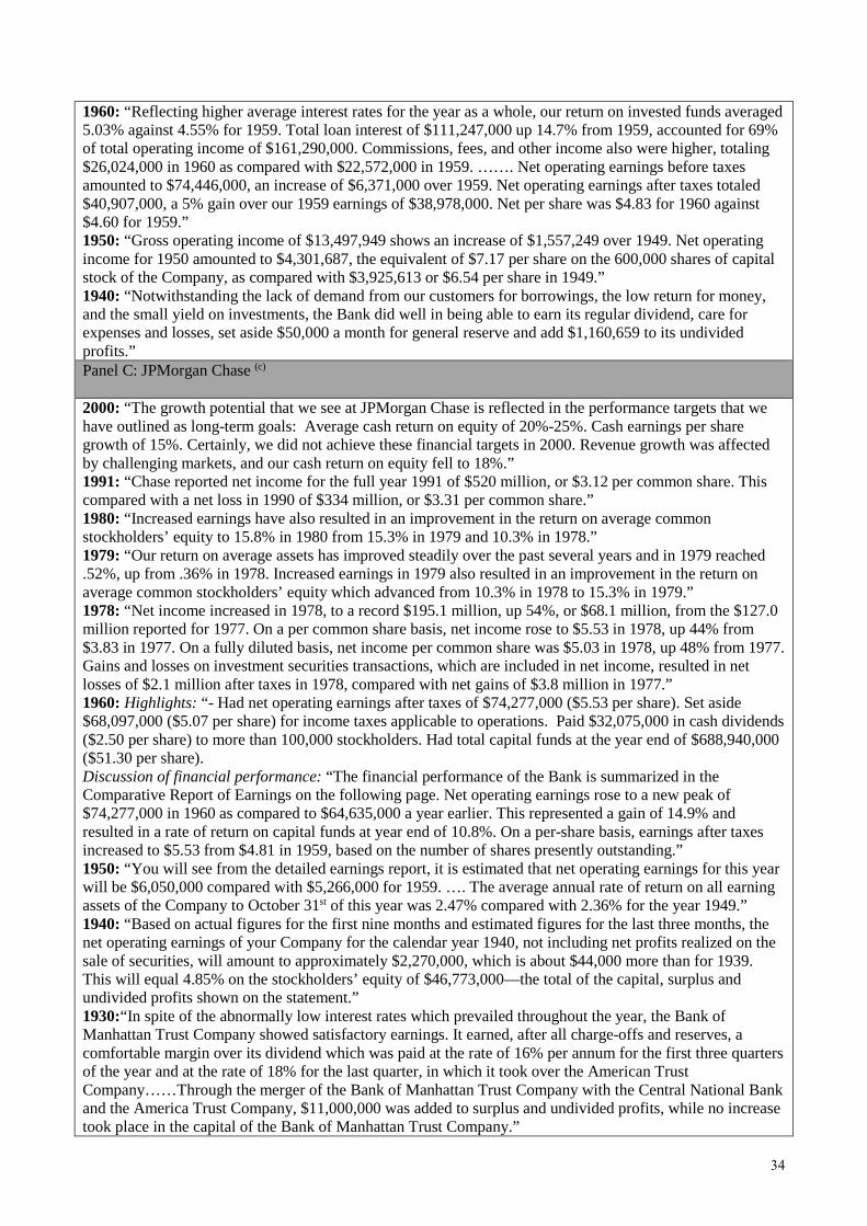
34

1960: “Reflecting higher average interest rates for the year as a whole, our return on invested funds averaged 5.03% against 4.55% for 1959. Total loan interest of $111,247,000 up 14.7% from 1959, accounted for 69% of total operating income of $161,290,000. Commissions, fees, and other income also were higher, totaling $26,024,000 in 1960 as compared with $22,572,000 in 1959. ……. Net operating earnings before taxes amounted to $74,446,000, an increase of $6,371,000 over 1959. Net operating earnings after taxes totaled $40,907,000, a 5% gain over our 1959 earnings of $38,978,000. Net per share was $4.83 for 1960 against $4.60 for 1959.” 1950: “Gross operating income of $13,497,949 shows an increase of $1,557,249 over 1949. Net operating income for 1950 amounted to $4,301,687, the equivalent of $7.17 per share on the 600,000 shares of capital stock of the Company, as compared with $3,925,613 or $6.54 per share in 1949.” 1940: “Notwithstanding the lack of demand from our customers for borrowings, the low return for money, and the small yield on investments, the Bank did well in being able to earn its regular dividend, care for expenses and losses, set aside $50,000 a month for general reserve and add $1,160,659 to its undivided profits.” Panel C: JPMorgan Chase (c)

2000: “The growth potential that we see at JPMorgan Chase is reflected in the performance targets that we have outlined as long-term goals: Average cash return on equity of 20%-25%. Cash earnings per share growth of 15%. Certainly, we did not achieve these financial targets in 2000. Revenue growth was affected by challenging markets, and our cash return on equity fell to 18%.” 1991: “Chase reported net income for the full year 1991 of $520 million, or $3.12 per common share. This compared with a net loss in 1990 of $334 million, or $3.31 per common share.” 1980: “Increased earnings have also resulted in an improvement in the return on average common stockholders’ equity to 15.8% in 1980 from 15.3% in 1979 and 10.3% in 1978.” 1979: “Our return on average assets has improved steadily over the past several years and in 1979 reached .52%, up from .36% in 1978. Increased earnings in 1979 also resulted in an improvement in the return on average common stockholders’ equity which advanced from 10.3% in 1978 to 15.3% in 1979.” 1978: “Net income increased in 1978, to a record $195.1 million, up 54%, or $68.1 million, from the $127.0 million reported for 1977. On a per common share basis, net income rose to $5.53 in 1978, up 44% from $3.83 in 1977. On a fully diluted basis, net income per common share was $5.03 in 1978, up 48% from 1977. Gains and losses on investment securities transactions, which are included in net income, resulted in net losses of $2.1 million after taxes in 1978, compared with net gains of $3.8 million in 1977.” 1960: Highlights: “- Had net operating earnings after taxes of $74,277,000 ($5.53 per share). Set aside $68,097,000 ($5.07 per share) for income taxes applicable to operations. Paid $32,075,000 in cash dividends ($2.50 per share) to more than 100,000 stockholders. Had total capital funds at the year end of $688,940,000 ($51.30 per share). Discussion of financial performance: “The financial performance of the Bank is summarized in the Comparative Report of Earnings on the following page. Net operating earnings rose to a new peak of $74,277,000 in 1960 as compared to $64,635,000 a year earlier. This represented a gain of 14.9% and resulted in a rate of return on capital funds at year end of 10.8%. On a per-share basis, earnings after taxes increased to $5.53 from $4.81 in 1959, based on the number of shares presently outstanding.” 1950: “You will see from the detailed earnings report, it is estimated that net operating earnings for this year will be $6,050,000 compared with $5,266,000 for 1959. …. The average annual rate of return on all earning assets of the Company to October 31st of this year was 2.47% compared with 2.36% for the year 1949.” 1940: “Based on actual figures for the first nine months and estimated figures for the last three months, the net operating earnings of your Company for the calendar year 1940, not including net profits realized on the sale of securities, will amount to approximately $2,270,000, which is about $44,000 more than for 1939. This will equal 4.85% on the stockholders’ equity of $46,773,000—the total of the capital, surplus and undivided profits shown on the statement.” 1930:“In spite of the abnormally low interest rates which prevailed throughout the year, the Bank of Manhattan Trust Company showed satisfactory earnings. It earned, after all charge-offs and reserves, a comfortable margin over its dividend which was paid at the rate of 16% per annum for the first three quarters of the year and at the rate of 18% for the last quarter, in which it took over the American Trust Company……Through the merger of the Bank of Manhattan Trust Company with the Central National Bank and the America Trust Company, $11,000,000 was added to surplus and undivided profits, while no increase took place in the capital of the Bank of Manhattan Trust Company.”

35

(a) Bank of Boston Corporation for 1985, First National Bank of Boston for the earlier years. (b) Chemical New York Corporation for 1985-1970, Chemical Bank & Trust Company for 1960-1940. (c) JPMorgan Chase for 2000, Chase Manhattan Corporation for 1991- 1960, Bank of Manhattan Trust Company for 1950-1930.

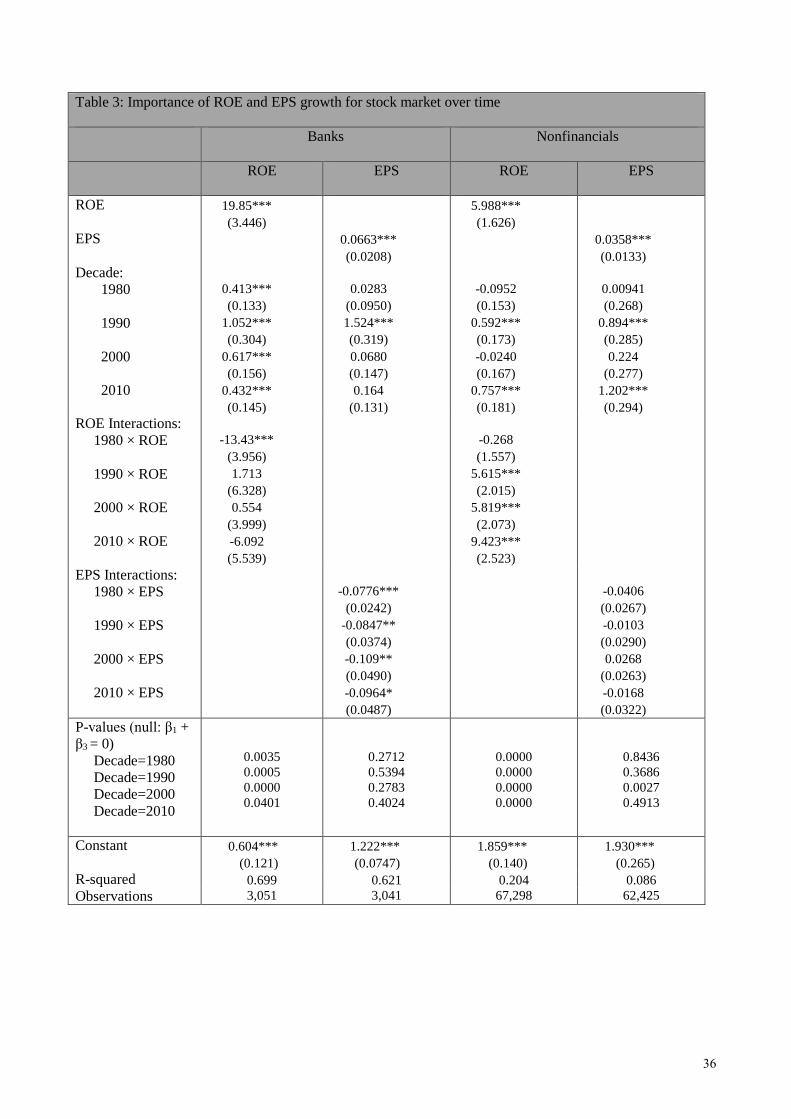
36

Table 3: Importance of ROE and EPS growth for stock market over time

Banks Nonfinancials

ROE EPS ROE EPS

ROE 19.85*** (3.446)

5.988*** (1.626)

EPS 0.0663*** (0.0208)

0.0358*** (0.0133)

Decade: 1980

1990

2000

2010

0.413*** (0.133)

1.052*** (0.304)

0.617*** (0.156)

0.432*** (0.145)

0.0283 (0.0950) 1.524*** (0.319) 0.0680 (0.147) 0.164

(0.131)

-0.0952 (0.153)

0.592*** (0.173) -0.0240 (0.167)

0.757*** (0.181)

0.00941 (0.268)

0.894*** (0.285) 0.224

(0.277) 1.202*** (0.294)

ROE Interactions: 1980 × ROE

1990 × ROE

2000 × ROE

2010 × ROE

-13.43*** (3.956) 1.713

(6.328) 0.554

(3.999) -6.092 (5.539)

-0.268 (1.557)

5.615*** (2.015)

5.819*** (2.073)

9.423*** (2.523)

EPS Interactions: 1980 × EPS

1990 × EPS

2000 × EPS

2010 × EPS

-0.0776*** (0.0242)

-0.0847** (0.0374) -0.109** (0.0490) -0.0964* (0.0487)

-0.0406 (0.0267) -0.0103 (0.0290) 0.0268

(0.0263) -0.0168 (0.0322)

P-values (null: β1 + β3 = 0) Decade=1980 Decade=1990 Decade=2000 Decade=2010

0.0035 0.0005 0.0000 0.0401

0.2712 0.5394 0.2783 0.4024

0.0000 0.0000 0.0000 0.0000

0.8436 0.3686 0.0027 0.4913

Constant 0.604*** (0.121)

1.222*** (0.0747)

1.859*** (0.140)

1.930*** (0.265)

R-squared 0.699 0.621 0.204 0.086 Observations 3,051 3,041 67,298 62,425

37

Table 4: Relative importance of ROE and EPS growth for banks’ and nonfinancials’ stock market

1 2 3 4

Bank -1.043*** (0.0773)

-0.635*** (0.0912)

ROE 10.92*** (1.156)

7.599*** (0.892)

Bank × ROE 10.85*** (3.152)

12.66*** (3.049)

EPS 0.0301** (0.0124)

0.0236*** (0.00675)

Bank × EPS -0.0477** (0.0241)

-0.0431** (0.0186)

Time FE Yes Yes Yes Yes Firm FE No Yes No Yes Constant 1.832***

(0.0443) 1.889*** (0.0271)

1.919*** (0.240)

1.968*** (0.141)

R-squared 0.111 0.379 0.093 0.423 Observations 70,349 70,349 65,466 65,466

38

Table 5: Growth in the number of shares vs. earnings growth.

Banks Non-Financials Banks Non-Financials

Earnings Growth dummies

Negative

Quartile 1

Quartile 2

Quartile 3

-0.0258*** (0.00795)

-0.0321*** (0.00882) -0.0223** (0.00889) -0.0245** (0.00939)

-0.00791*** (0.00143)

-0.00559*** (0.00102)

-0.00341*** (0.00107) 0.000955 (0.00119)

-0.0271*** (0.00762)

-0.0318*** (0.00880) -0.0216** (0.00926) -0.0239** (0.00960)

-0.00758*** (0.00146)

-0.00535*** (0.00103)

-0.00388*** (0.00118) 0.000501 (0.00128)

Time FE Yes Yes Yes Yes Firm FE No No Yes Yes Constant 0.0873*

(0.0452)

0.00825** (0.00343)

0.0865* (0.0451)

0.00855** (0.00331)

R-squared 0.101 0.017 0.104 0.023 Observations 3,135 64,801 3,135 64,801 The dependent variable is the log of quarterly growth in the number of shares. Negative is equal to 1 if the contemporaneous quarterly earnings were negative. Quartile i, with i=1,2 and 3 are dummy variables equal to one if the contemporaneous quarterly earnings were in the first, second and third quartile of the distribution of positive earnings, respectively. The omitted group are the firms with earnings in the fourth quartile.